Estimating the Cost of Debt - Australian Competition and ... Development... · Current regulatory...

Regulatory Development

Estimating the Cost of Debt A Possible Way Forward

April 2013

ii

Regulatory Development Branch, Australian Competition and Consumer Commission

The Regulatory Development Branch within the Australian Competition and Consumer Commission (ACCC) and Australian Energy Regulator (AER) was established in 2006 to increase the quality of economic analysis available to the ACCC/AER and promote the consistent use of economic principles across the different sectors subject to economic regulation.

The economic regulation of infrastructure is a relatively new area of activity in Australia and was integral to the implementation of the National Competition Policy. As the regulatory task undertaken by the ACCC/AER has developed there has been an increased need for input from specialist regulatory economists.

In response the ACCC established a group of economic specialists to

• provide wide ranging economic

advice

• research and develop best practice

regulatory techniques

• contribute to economic discussion,

debate and training regarding

regulatory issues.

The promotion of the use of best practice economic principles recognises that while the principles of regulation might have specific applications across the diversity of areas regulated by the ACCC/AER they are broadly shared. The Branch keeps abreast with latest thinking in regulatory economics and develops shared regulatory principles for the different sectors that the ACCC/AER regulates.

In addition the Regulatory Development Branch has responsibility for a number of external activities such as the ACCC/AER annual Regulatory Conference, the Utility Regulators Forum, the Infrastructure Consultative Committee and the ACCC/AER Working Paper series.

The following paper is part of the Regulatory Development Branch’s commitment to contribute and foster discussion on regulatory economic issues.

Henryk Smyczynski

Economic Adviser


ACCC and AER

Igor Popovic

Principal Economic Adviser


ACCC and AER

The views expressed in this paper are those of the authors and not necessarily those of the ACCC or the AER.

iii

Table of Contents

1. Introduction ............................................................................................................................ 1

2. Current regulatory practice in estimating the cost of debt .................................. 3

3. Issues with the current approach .................................................................................. 4

3.1. Five year regulatory period vs. ten year cost of debt assumption ............. 5

3.2. Investment distortions ............................................................................................... 7

3.3. Concerns about Bloomberg Fair Value curve .................................................... 8

4. What is the cost of debt of a regulated firm? ........................................................... 10

5. Portfolio approach ............................................................................................................. 14

5.1. Portfolio approach with annual adjustments .................................................. 14

5.2. Generalised form of the portfolio approach with annual adjustments.. 18

5.3. Potential concerns over the portfolio approach ............................................. 19

5.4. Portfolio approach with no annual adjustments ............................................ 19

5.5. Should the portfolio approach apply to the credit margin or total cost of debt? ................................................................................................................................ 20

5.6. Allowing options to regulated businesses ........................................................ 25

5.7. Annual adjustment ..................................................................................................... 26

5.8. Weights within the portfolio approach .............................................................. 36

5.9. Conclusion on the portfolio approach ................................................................ 39

6. Estimating the benchmark .............................................................................................. 40

6.1. Creating a new cost of debt benchmark ............................................................. 40

6.2. Using a commercial data provider ....................................................................... 42

6.3. Conclusion on estimating the benchmark ......................................................... 45

7. Transitional arrangements ............................................................................................. 45

8. A worked example .............................................................................................................. 48

9. Other forms of financing .................................................................................................. 49

10. The averaging period over which the cost of debt should be estimated ...... 53

11. Conclusion ............................................................................................................................. 54

1

1. Introduction

The Weighted Average Cost of Capital (WACC) is the basis for most regulators’ determination of a firm’s required return on capital, which is a component of the firm’s total revenue requirement. The cost of debt is a large component in calculating the firm’s WACC. As a result, the cost of debt is positively correlated to the price of regulated services, and seemingly small changes in its estimate can have a large impact on the firm’s cash flows. Cost of debt estimation methodologies and their application have therefore been subject to intense debate. This paper aims to resolve a number of issues that have emerged from that debate by proposing a new approach to determining the cost of debt, which balances benchmark and efficiency incentives with the reality of debt issuance practices of regulated firms.

In developing this proposed new approach, the paper aims to reach a pragmatic solution to balancing competing interests. While regulated entities require adequate compensation for their investment and seek to minimise their business risk, consumers may seek price certainty and low price volatility. As well regulators aim to address their regulatory criteria and seek to strike an appropriate balance of predictability, transparency, accuracy and flexibility. Balancing these interests is important when assigning and adequately pricing risk, and determining the cost of debt.

Much of the debate in cost of debt estimation has occurred within the scope of the Australian Energy Regulator’s (AER’s) revenue resets for regulated energy infrastructure. Under the current approach, the AER estimates the cost of debt for regulated businesses as the prevailing cost of debt at the start of an access arrangement period. The benchmark cost of debt for energy businesses is currently estimated using the Bloomberg Fair Value curve. Recently, due to the perceived unreliability of the Bloomberg Fair Value, the AER has attempted to depart from relying solely on Bloomberg estimates and has used a range of additional estimates. However, the Australian Competition Tribunal (the Tribunal) has not been satisfied with this approach.

The Tribunal has advised the AER that if it considers the Bloomberg Fair Value estimate to be unreliable, then the AER should develop an alternative coherent and consistent methodology in consultation with stakeholders.1 This paper aims to meet this challenge by setting out a methodology for use in future pricing that can be used by Australian regulators.

To adequately compensate a regulated business for the cost of its debt capital over an access arrangement period, the estimate should reflect the expected cost

1 Australian Competition Tribunal, Application by Envestra Ltd (No 2) [2012] ACompT 3, p. 20.

2

of debt that an efficient regulated business will be exposed to over that period.2 The cost of debt forecast should include the return required by debt capital providers plus all expected transaction costs associated with raising this capital.

Under the current regulatory framework, regulated businesses have an incentive to minimise their actual cost of debt, given that over any particular access arrangement period businesses keep the difference between their actual cost of debt and the forecast included in regulatory pricing. Further, in the absence of refinancing risk, under the current regulatory framework regulated businesses may have an incentive to issue all of their debt at the start of the access arrangement period with a term equal to the length of that period, thereby hedging their interest rate risk exposure.

However, regulated businesses also face refinancing risk – the risk that they will not be able to roll-over their debt when it comes due. Therefore it may not be prudent for businesses to refinance all of their debt at the start of the access arrangement period. Instead regulated businesses may limit the amount of debt they have to refinance in any given year and spread their borrowings over time.

On any given date, regulated businesses have a portfolio of debt that was raised at different points in time. As a result, the regulated businesses expected cost of debt over the access arrangement period is a function of the existing cost of debt, the prevailing cost of debt at the start of the period and the expected cost of future debt issued during the access arrangement period.

This paper argues that the cost of debt for regulated businesses could be estimated using a debt “portfolio approach” without annual adjustments. This approach requires the estimated cost of debt over the access arrangement period to be determined as the average benchmark cost of debt an efficient firm would face at the start of the access arrangement, where the averaging period is equal to the benchmark term of debt. While it is possible to adjust the cost of debt annually within the access arrangement period, the paper argues that on balance such adjustments are not advantageous to the regulatory process.

It is also argued that regulated businesses should not be provided with a choice of either the approach, the method in implementing the approach or of variables used. Providing choices may result in an incentive for regulated businesses to select options that lead to highest revenue and not those that represents debt practices of efficient regulated businesses. Further, allowing a choice may result in multiple benchmarks being created, and it may remove the incentive to act efficiently.

2 In theory, where a revenue decision is being made for a given investment, the cost of

capital should be the cost of capital for the given investment. Where the firm only operates in one area such as gas transmission this could reasonably be assumed to be the overall cost of the firm’s capital. However, where the firm operates across multiple areas this is unlikely to be the case. In this situation, awarding each project the firm’s overall cost of capital will adequately reward a firm for its overall cost of capital (on existing projects) if all the firm’s investments are regulated, although it may discourage investment in capital that has a higher average capital cost than the firm’s overall WACC. In the event a firm has a significant proportion of its operations in non regulated areas, then awarding a firm its overall cost of capital on regulated investments is unlikely to appropriately compensate the regulated firm.

3

Finally, it is argued that the cost of debt forecast should not be adjusted within an access arrangement period through the annual tariff adjustment mechanism. Under the portfolio approach, the cost of debt that is not accounted for within the current period is accounted for in the following access arrangement period. Further, constant weights should be used in the “portfolio approach”. This is because using expected debt issuance weights from the Post Tax Revenue Model does not eliminate investment distortions given regulated businesses can deviate away from their expenditure forecasts.

Other parts of this paper discuss the appropriate method for estimating the benchmark cost of debt, and consider other forms of financing, transitional arrangements, and the averaging period.

Finally, a brief comment on the nomenclature used in this paper. The term “cost of debt”, used throughout this paper, should be taken to mean the “required rate of return on debt” as it is this rate that regulatory criteria and regulatory pricing methodologies require as an input into price determinations. This is the rate required by debt holders to provide or continue to provide debt capital to regulated firms.

Further, while this paper uses the term “portfolio approach” to estimating the cost of debt, similar approaches have been sometimes called “historic average” or “trailing average” approaches. However, it is felt that the later terminology does not adequately capture the forward-looking nature of the cost of debt estimate under the portfolio approach. While some of the debt considered relevant under this approach is already issued at the time of the access arrangement period (and can be thought of as historic), it is forward-looking in that it is still current in the forward looking regulatory period.

2. Current regulatory practice in estimating the cost of debt

Current regulatory practice, following the decision by the Australian Competition Tribunal in Application by GasNet Australia (Operations) Pty Ltd [2003] ACompT 6 (23 December 2003) (“GasNet”), sets the cost of debt for an access arrangement period by adding the debt margin of a 10-year corporate bond with a credit rating equal to the debt proxy to the yield to maturity on a 10-year Commonwealth Government security. Debt issuance costs are usually added to this rate (alternatively they are accounted for in operating expenditure).

The current practice can be shown algebraically as:

Equation 1

DICDRPrrE fd )(

Where:

)( drE = the expected cost of debt of the regulated firm;

4

fr = risk-free rate currently set at the yield to maturity on 10-year

Commonwealth Government Bonds;

DRP = debt risk premium currently set on the 10-year corporate bonds with a credit rating equal to the credit rating of the debt proxy less the yield to maturity on 10-year Commonwealth Government bonds; and,

DIC = the issue costs an efficient firm expects to incur in raising its debt capital.

Equation 1 can be expanded and simplified as follows:

Equation 2

DICrYTMrrE ffd )()( 10

DICYTMrE d 10)(

Where: 10YTM = yield on 10-year corporate bonds with a credit rating equal

to the credit rating of the proxy of an efficient firm.

At the moment, corporate debt fair yields of the relevant credit rating are sourced from the Bloomberg professional data service.

3. Issues with the current approach

The method of implementing the current approach for setting the cost of debt varies across the ACCC and AER. At the time of writing this paper, the cost of debt for energy businesses is determined by the AER with reference to the prevailing fixed 10-year BBB+ cost of debt at the start of an access arrangement period. The fixed 10-year BBB+ rate is determined by the 7-year extrapolated BBB Bloomberg Fair Value estimate. On the other hand, in communications regulation, the ACCC estimates Telstra’s cost of debt with reference to Telstra’s own 10-year, A-rated bond.

However, there are a number of issues with the construct and implementation of the current approach. For example, it is not clear how a regulated business can hedge its debt exposure if it actually issues 10-year debt while the regulator resets the cost of debt allowance every 5 years. The current approach also does not take account of the cost of debt within the access arrangement, which may expose regulated businesses to risk if the businesses needs to raise funds within the access arrangement and the actual cost of debt were to increase significantly above the approved cost of debt within that period. Further, currently there are questions over the general accuracy of the Bloomberg Fair Value estimate and its appropriateness for use in a regulatory context.

5

3.1. Five year regulatory period vs. ten year cost of debt assumption

Under the current regulatory framework if a regulated business’s actual performance over the access arrangement conforms to the benchmark assumptions, the regulated business should satisfy the NPV=0 condition.3 Alternatively, if the regulated business outperforms (underperforms) the benchmark assumption the business should obtain a positive (negative) NPV outcome.

However, if a regulated business were to issue all of its debt at the start of the access arrangement, with the benchmark characteristics (10-year, fixed, BBB+, Australian bond), it is not clear the NPV=0 condition would be satisfied. By issuing 10-year BBB+ debt at the start of the access arrangement, the regulated business is exposed to risk at the start of the next access arrangement as the cost of debt is reset at that time –every 5 years and not every 10 years. For example, if the regulated business was to issue 10-year debt at the start of the access arrangement period and that issue comprised its entire debt portfolio, it would possess a natural hedge between its debt related cost and revenue over the next 5 years.

Figure 1

For the first access arrangement, the business satisfies the NPV=0 condition as its debt cost are equal to the building block compensation for the cost of debt. However, given that none of the regulated business’ debt expires at the start of the next access arrangement (existing 10-year debt is only half way to maturity),

3 NPV = Net Present Value, which is the net value of future cash flows (outflows and

inflows) discounted into their value today.

6

the regulated business does not need to refinance. Therefore, its actual cost of debt does not change between the two access arrangement periods.

However, under the current regulatory framework the regulator will reset the regulated business’ revenue accounting for the prevailing cost of debt at the start of the next access arrangement. The regulated business may not satisfy the NPV = 0 condition. If the prevailing cost of debt at the start of the second access arrangement period is lower than the cost of debt that existed at the start of the first period, the NPV will be negative. As the regulated business has locked in the higher cost of debt in the earlier access arrangement and the new revenue is determined according to the new and lower cost of debt, the regulated business will be undercompensated.

However, the NPV can be positive if the cost of debt in the second access arrangement period is higher than the prevailing cost of debt at the start of the first period (see Figure 2). It should be noted that this risk is not eliminated by prematurely expiring 10-year debt when it has 5 years to maturity.

Figure 2

Assuming there is no refinancing risk, a way a regulated business can hedge its cost of debt exposure over the access arrangement period is to issue all its debt at the start of the access arrangement with a maturity that is equal to the access arrangement period. Under this strategy, all of the regulated business’ debt matures at the end of the access arrangement period and is refinanced at the same time that the regulator estimates the regulated business’ new cost of debt allowance.

7

However, under this strategy it is expected the regulator would overcompensate the regulated business. If the yield curve is on average upward (downward) sloping, the mismatch between the access arrangement period and the term of debt will result in a long term expectation of a positive (negative) NPV. As, on average, the yield curve is upward-sloping, and the 10-year debt is more expensive than 5-year debt, the regulated business can expect to over-recover its costs over the long term.

To address these shortcomings, the regulator can ensure the benchmark term of debt and the length of the access arrangement are aligned. Alternatively, it could implement a different method to calculate the cost of debt for regulated businesses. This paper advocates that a different method is warranted and that the cost of debt over the access arrangement can be estimated using the portfolio approach with no annual adjustments.

3.2. Investment distortions

Another identified shortcoming of the current regulatory framework is that it sets the cost of debt based on the prevailing cost of debt at the start of an access arrangement period and it does not take account of the cost of debt within the access arrangement. The risk with such an approach is that the regulated business may have to issue debt within the access arrangement and be exposed to the risk that cost of debt within the access arrangement will be significantly different to the cost of debt that prevailed at the start of the access arrangement.

For example, assume in year 2 of a 5-year access arrangement a regulated business has to undertake large capital expenditure and in that year the prevailing cost of debt is abnormally high. Given the regulated business needs to issue debt to fund the large capital expenditure, the high cost of newly issued debt may make the project unprofitable as the regulator compensates the business for the cost of debt at levels prevailing at the start of the access arrangement. As a result, the regulated business may delay the capital expenditure in year 2 of the access arrangement, to a time when the cost of debt is more favourable.

8

Figure 3

3.3. Concerns about Bloomberg Fair Value curve

A final key issue with the current approach to setting the cost of debt is that since the Global Financial Crisis concerns arose around the use of extrapolated Bloomberg estimates, with the extrapolated 10-year BBB Bloomberg Fair Value providing an abnormally high estimates, when compared with actual bond data. As is evident in Figure 4 below, during the post Global Financial Crisis period the 10-year BBB Bloomberg Fair Value has deviated significantly away from the average yields on corporate bonds with a BBB credit rating and an average maturity of 10 years.4

Further, when the 10-year BBB Bloomberg Fair Value rate is contrasted with regulated businesses actual cost of debt, the 10-year BBB Bloomberg Fair Value appears to over-compensate the service provider for its actual cost of debt. This is not to say the 10-year BBB Bloomberg Fair Value was necessarily appropriate in the period before the Global Financial Crisis.5

4 Bonds considered were those with maturity of between 8 and 12 years.

5 In the pre-Global Financial Crisis period, there was ongoing contention between the use of CBA Spectrum data or the Bloomberg Fair Value. However, this issue is no longer present as the CBA Spectrum has ceased publishing its yield curves.

9

Figure 4

As a result of its concerns over the 10-year BBB Bloomberg Fair Value, the AER has recently attempted to adjust the Bloomberg Fair Value to account for the overcompensation in the post Global Financial Crisis period.6 However, the AER’s decisions to adjust the Bloomberg Fair Value have been successfully appealed by regulated businesses, effectively leaving the regulator with the following options:

Continue estimating the cost of debt using the 7-year BBB Bloomberg Fair Value extrapolated to 10 years.

Use the bond yield approach developed by the Economic Regulation Authority (ERA) which was upheld by the Tribunal.

Create a new methodology for calculating the cost of debt with consultation from market participants.

Of greater concern when using Bloomberg Fair Value curves to estimate the 10-year cost of debt is that currently there is no 10-year BBB Bloomberg Fair Value - i.e. the BBB Bloomberg Fair Value curve does not extend to ten years. As a result, the 10-year BBB Bloomberg Fair Value has to be extrapolated from available Bloomberg data sources. Some common methods used to extrapolate include using:

A linear relationship between the 5-year BBB Bloomberg Fair Value and 7-year BBB Bloomberg Fair Value to extrapolate the 10-year BBB value.

The difference between the 10-year AAA and 7-year AAA Bloomberg Fair Value is added to the 7-year BBB figure to approximate the 10-year BBB value.7

6 The AER adjusted the Bloomberg Fair Value by averaging it with a bond yield that closely

matched the benchmark characteristics (10 year maturity, BBB+, operated in the regulated industry).

7 Bloomberg’s decision to cease publishing a 10-year AAA Bloomberg Fair Value rate has resulted in the AER being unable to use it primary method to extrapolate from the 10-

10

Paired bond yield analysis.

The difference between US 10-year and the US 7-year BBB Bloomberg Fair Value swapped into Australian dollars, and adding that amount to the 7-year Australian BBB Bloomberg Fair Value.

Extrapolating based on Bloomberg Fair Value data to approximate a 10-year rate is not ideal as it introduces another level of uncertainty in the cost of debt estimate. The extrapolation methods are not perfect and can misestimate the 10-year cost of debt.

There are additional concerns relating to the Bloomberg Fair Value. For example, it:

is not specific to a particular credit rating but specific to a band of credit ratings. For example, there is no BBB+ Bloomberg Fair Value which is needed for regulatory purposes; instead there is a BBB Bloomberg Fair Value which includes BBB-, BBB, and BBB+ rated debt. Given the BBB+ cost of debt forecast is required, the BBB Bloomberg Fair Value will overestimate the cost of debt.

includes subordinate and callable debt. In particular subordinated debt of an insurance company (with no tangible assets) is not representative of the cost of a typical regulated business.

excludes some forms of debt e.g. floating rate notes.

4. What is the cost of debt of a regulated firm?

As outlined earlier, there are significant problems with the current approach for estimating the cost of debt. This paper attempts to propose a new cost of debt methodology that could be used by various regulatory bodies. The paper argues that the cost of debt could be estimated using the portfolio approach with no annual updates.

Under the current regulatory framework regulated businesses receive a fixed allowance for their cost of debt at the start of the access arrangement period. If the regulated businesses issue debt within the access arrangement at a rate below the allowance, they keep the benefit. Conversely, if regulated businesses issue debt within the access arrangement above the allowance, they bear the additional costs. As a result, regulated businesses have an incentive to minimise their actual cost of debt.

Due to this incentive, it can be assumed that some of the past practices of debt issuance by regulated businesses were efficient and can be used as a proxy to estimate future efficient practices. However, when using past practice as a proxy for future practices, one first needs to be determine whether the past actions are likely to be representative of the future.

It is expected that efficient businesses will over time take a dynamic approach to debt financing. At any given point in time businesses consider all debt financing

year rate (extrapolation method of adding the difference between the 10 and 7 year AAA rate to the 7 year BBB rate).

11

options and select the option that results in the lowest cost of debt over the long term (see section 9). Therefore a debt practice that was efficient in the past may not be efficient in the future. For example, prior to the onset of the Global Financial Crisis, it was efficient for utilities to credit wrap their debt. However, estimating the cost of debt today using yields on credit wrapped bonds would not result in an efficient cost of debt estimate.8

Further, when determining a new regulatory cost of debt approach, debt practices which are a product of the regulatory environment should be ignored. This is because these practices will change if the regulatory environment changes. If in setting a new regulatory framework, a regulator considers debt practices that are a result of businesses reacting to the existing regulatory framework, it may create a self fulfilling method that may not necessarily be efficient.

For example, a number of businesses are currently able to lock in part of their cost of debt for the access arrangement period using swap contracts. This debt practice could be used to justify the 5-year prevailing cost of debt benchmark. However if the regulator were to increase the access arrangement from 5 years to 6 years, it could become efficient for the business to enter 6-year swaps rather than 5-years swaps.

The use of swap contracts to lock in the cost of debt for the access arrangement is a consequence of the regulatory framework, and their use by regulated businesses would change if the regulatory framework were to change. Ideally the regulatory framework for the cost of debt should reflect the efficient debt practices that occur in a competitive market. This would align competitive incentives with regulatory incentives.

Over time, the regulatory forecast should be updated to reflect the most recent efficient debt practices of regulated businesses.9 This is essential in order to ensure the benefits associated with the most efficient debt structure are passed on to users. The frequency with which the forecasts are updated will determine the strength of incentives the regulated businesses has to implement the most efficient debt structure.

For example, if the cost of debt is reviewed frequently the businesses might not have a strong incentive to implement the most efficient cost of debt strategy as they only keep the gain for a short period of time. However, if the review is less frequent, the businesses will have a stronger incentive to minimise their cost of debt since they keep the savings for a longer period of time.

Under the current regulatory framework it can be shown, given a number of assumptions (most importantly the assumption that there is no refinancing risk), that the optimal strategy for regulated businesses is to issue all of their debt at the start of the access arrangement period and with a term equal to that period.

8 Prior to the GFC the process of credit wrapping bonds was an efficient process. Business

could use a monoline to insure their bonds, effectively giving the bonds a higher credit rating and subsequently a lower yield. However, following the GFC majority of the monolines lost their AAA credit rating and could not longer credit wrap the bonds.

9 For the AER area this could be at every WACC Review.

12

This is a consequence of the current regulatory framework, which provides a fixed forward looking cost of debt allowance over an access arrangement period.

If a regulated business locks in the cost of debt at the start of the access arrangement it would, on average, be compensated by the regulator for at least the cost it incurs.10 The strategy is demonstrated graphically below in Figure 5. At the start of the access arrangement the regulated business enters into fixed 5-year debt and its cost is represented by the red line.

The building block revenue compensates the regulated business with a 10-year forward looking debt, and the expected compensation the regulated business receives is depicted by the green line. Under this strategy the business is not exposed to any risk over the access arrangement. There is no uncertainty as to the gap between the cost of debt and the compensation the regulated business receives from the regulator. Figure 5 illustrates that under this strategy the business is over compensated as on average 10-year debt has a higher yield than 5-year debt.

Figure 5

However, regulated businesses have argued that they do not issue all of their debt at the beginning of the access arrangement with a maturity equal to the period of regulation. Regulated businesses state that having all of their debt mature at the end of the access arrangement and having to refinance all of their

10 The business is compensated for a 10-year cost of debt, while it is exposed to 5-year

debt. As, on average, the yield curve is upward slopping yield curve, the business is expected to be over compensated over the long term.

13

debt at the start of the access arrangement would expose them to significant refinancing risk.

While the current regulatory framework provides the regulated business with an incentive to issue all of its debt at the start of the access arrangement with a term of debt equal to the period of regulation, refinancing risk creates a counterbalancing incentive for the business to:

limit the percentage of debt refinancing in any particular year

issue debt with a longer term.

Given the current incentives in the regulatory framework and the given that regulated businesses do not issue all of their debt to match the regulatory period, one can conclude that it is efficient for a regulated business to spread its borrowing over time rather than to issue all of its debt at the start of the access arrangement.

Consider an example of the regulated business that refinances 20 % of its debt every year with 5-year debt and the regulator compensates the regulated business, over the access arrangement using the prevailing cost of debt at the start of the access arrangement. Under such an arrangement the regulated business would have an annual cost of debt and annual debt reimbursement profile as outlined in Figure 6 below.

Figure 6

In this scenario the regulated business’s cost of debt does not closely match the regulatory allowance. As illustrated Figure 6, the regulated business’ cost of debt is not aligned with the compensation it receives for debt in the allowed revenue. There is a mismatch which exposes the regulated business to risk. In some

14

periods the regulated business will be over-compensated and in others under-compensated.11

The cause of the mismatch is that the debt profile assumed by the regulator is not the same profile implemented by the regulated business. If the regulator were to set the estimate of the cost of debt on an average of the historical cost of debt and the prevailing cost of debt at the start of access arrangement and within the access arrangement (portfolio approach) the mismatch could be minimised. Using the portfolio approach would compensate a service provider for its efficient benchmark cost of debt more accurately.

Given the incentives in the regulatory framework and financing risks faced by businesses such practice could be considered efficient. As a regulator is required to model the cost of debt using efficient debt profiles it can estimate the cost of debt using a portfolio approach. However it will be argued the regulator should not apply annual adjustment within the access arrangement period (see section 5.7).

5. Portfolio approach

An approach to determining the regulatory cost of debt (or the required rate of return on debt) that replicates debt issuing practices of an efficient firm can recognise the staggering of debt issuances. The approach is termed the portfolio approach and this section examines the issues surrounding its implementation. It is argued that the cost of debt can be set based on the portfolio approach without any annual adjustments. Further it is argued that the assumed term of debt can equal the industry average and that each year the firm can be assumed to refinance an equal proportion of its debt.

5.1. Portfolio approach with annual adjustments

To illustrate how a portfolio approach can be implemented, consider an example of a business that staggers its debt. Consider a business that issues only domestic 5-year fixed rate debt12 and each year 20 % of debt matures and is refinanced with new 5-year debt. For simplicity it is assumed no derivative contracts are used13 and capital expenditure and depreciation are equal to zero, resulting in a constant capital base over time.

This strategy is illustrated by Figure 7 below. Each horizontal line represents one issuance of fixed debt where the line begins at the year the debt was issued and ends on the year that debt matures.

11 In Figure 6 the service provider is over compensated for the years 2005, 2006, 2007,

2008 and under-compensated for the years 2009, 2010.

12 The time to maturity would have to be estimated empirically. However, 5 years is assumed for computational simplicity. It is also assumed that firms do not engage in alternative sources of financing (international debt, variable debt, etc).

13 This will be further discussed in the next section.

15

Figure 7

The business’s cost of debt for any given year is the average cost of the various debt issuances (represented by the horizontal lines that intersect the year in question). For example, the first year’s cost of debt can be determined by assigning 20 % weight each to costs of fixed rate debt entered into four, three, two and one year prior to, as well as at the commencement of the access arrangement period.

All components of the cost of debt in the first year of the access arrangement period are known at the start of the period. The cost of debt in the first year is a mixture of pre-existing debt and forward looking debt. While the cost of debt exposure of the regulated business in the first year of the access arrangement period is primarily drawn from pre-existing debt (80 % of debt is pre-existing and 20 % of debt is issued at the start of the regulatory period), it remains forward-looking in a sense that it is the cost of debt the business will face over the upcoming access arrangement period.

It is worth pointing out that a practical problem exists with regard to estimating the first year’s cost of debt at the start of a new access arrangement period. At the time the final decision is made, the five year cost of debt at the start of the period is not known.14 As a result, 20 % of the parameters (i.e. the five year cost of debt at the start of the period) for determining the cost of debt are not known at time of the final decision. This issue will be further discussed in section 10, which outlines the averaging period over which the cost of debt could be estimated. However, in this example, for simplicity it will be assumed the final decision date and the commencement date of the access arrangement are aligned so that all parameters are known.

14 Final decision is usually made 3 months prior to commencement of the access

arrangement period.

16

Mathematically the cost of debt in the first year of the access arrangement period is:

Equation 3

0TC1 =

-4R1 +

-3R2 +

-2R3 +

-1R4 +

0R5

Where:

aTCb = Regulated businesses total cost of debt for the period a to b.

aRb = Cost of debt that was entered into in year a and matures in year b

In the second year of the access arrangement period, the fixed rate debt that was entered into four years before the start of the period matures and has to be rolled over into a new 5-year debt that matures six years from the start of the period (or 1st year of the next access arrangement). The second year’s cost of debt can be determined by assigning 20 % weight each to costs of fixed rate debt entered into three, two and one year prior to the access arrangement period, and 20 % each to cost of debt at the commencement of and one year into the period.

Given that at the start of the access arrangement the regulator does not know, with certainty, what the 5-year cost of debt is going to be in one year’s time, 20 % of the second year’s cost of debt is determined by parameters that are not known at the time of the reset (represented with parameter highlighted in red). The cost of debt of the regulated business in the second year of the access arrangement is still primarily debt that was entered into prior to the commencement of the period, but this falls to 60 %:

Equation 4

1TC2 =

-3R2 +

-2R3 +

-1R4 +

0R5

1R6

Note the inputs that appears in green represents data that is known at the start of the access arrangement period, and the inputs highlighted in red represents data that is unknown at the start of the access arrangement period.

The process of rolling over debt on an annual basis continues throughout the access arrangement period. As a result, the estimate of third year’s cost of debt is:

Equation 5

2TC3 =

-2R3 +

-1R4 +

0R5

1R6 +

2R7

while in the fourth and final years of the period estimates of the cost of debt are:

17

Equation 6

3TC4 =

-1R4 +

0R5

1R6 +

2R7 +

3R8

Equation 7

4TC5 =

0R5

1R6 +

2R7 +

3R8 +

4R9

Assuming the capital base is constant, and assuming no capital expenditure or depreciation, the arithmetic average annual cost of debt faced by the regulated business over the access arrangement period is:

Equation 8

0TC5 =

-4R1+

-3R2+

-2R3+

-1R4+

0R5+

1R6+

2R7+

3R8+

4R9

The above relationship defines the portfolio approach with annual adjustment when the benchmark term of debt is equal to 5 years.

Under Equation 8, the average annual cost of debt over the access arrangement period is a mixture of debt that was entered into after the start of the period (40 %), debt that was entered into at the commencement of the period (20 %) and pre-existing debt (40 %).15 Therefore, only 60 % of the data required to compute the average cost of debt is available when the cost of capital is set.16

Figure 8 is a graphical representation of data availability. The debt represented by a green line denotes data that is available at the start of the access arrangement, while red signifies data that is unavailable at the start of that period.

15 The percentages assume that each input in the formula has an equal weighting. Debt that

is entered into after the commencement of the access arrangement is:

1r6, 2r7, 3r8, 4r9.

Historical debt is debt that is entered into prior to the commencement of the access arrangement period. The historical debt is represented by:

-4r1, -3r2, -2r3, -1r4 I.e. starting dates are -1

16 Data that is available when cost of capital is set – at the start of the access arrangement

is: -4r1, -3r2, -2r3, -1r4, 0r5 – i.e. starting dates are 0

18

Figure 8

5.2. Generalised form of the portfolio approach with annual adjustments

Equation 8 describes the portfolio approach under the 5-year term assumption. The generic equation for the portfolio approach with annual adjustments can be defined as:

Box 1

As regulated businesses do not issue all of their debt at the start of the access arrangement period but rather stagger their debt issuance over time, the cost of debt could be based on an average of:

Equation 9

Where:

0TCt Total cost of debt for the period beginning in time 0 and ending in period t, where t is the length of the access arrangement period.

aRb: Actual return on debt that was entered into in year a and matures in year b

t: Years in access arrangement

19

The fixed cost of debt that was entered prior to the commencement of the access arrangement period, but has not matured

The fixed cost of debt that will be entered into during the access arrangement period.

There are two key questions to answer in setting the cost of debt under the portfolio approach. The first relates to the method of estimating the cost of debt benchmark. The second relates to the averaging period and, subsequently, the frequency of debt refinancing.

The cost of debt estimate can reflect a benchmark credit rating of regulated businesses and the benchmark term of debt, with the term related to the averaging period and frequency of refinancing. Options for method of estimating the benchmark are further discussed in section 6.

The averaging period for the cost of debt can equal the past average term of debt issued by the regulated businesses in that industry. If regulated businesses are implementing a portfolio approach when sourcing debt financing and are on average acting efficiently, then setting the averaging period and refinancing frequency according to the industry average term of debt can be expected to satisfy the NPV=0 condition.

5.3. Potential concerns over the portfolio approach

An argument against using the portfolio approach is that it may not be consistent with the ‘build or buy’ framework. For example, if the current cost of debt is higher than the average of existing cost of debt, a new entrant would find it unprofitable to compete with the incumbent regulated business as the total revenue would be insufficient to compensate the new entrant for the cost of new debt it has to issue at the start of the access arrangement period. This is because a new entrant must issue all its debt at the beginning of the period. The opposite would apply if the current cost of debt were lower than the average cost of existing debt, where the new entrant would have a competitive advantage over the incumbent regulated business.

A similar concern may arise with regard to new investment by the regulated business. As the portfolio approach does not mimic the prevailing cost of debt financing, regulated businesses may have a disincentive to invest at times when the current cost of debt is higher than the estimate under the portfolio approach. On the other hand, they may overinvest at times when the prevailing cost of debt is lower than the portfolio approach estimate.

5.4. Portfolio approach with no annual adjustments

The remainder of this paper examines the appropriate methods in implementing the portfolio approach in more detail, including whether under this approach the averaging should apply to the total cost of debt or only the credit margin. Further, the annual adjustment and weighting scheme in the portfolio approach are discussed.

Specifically, the paper argues that the cost of debt should not be adjusted annually within the access arrangement period. Employing this version of the portfolio approach will limit the data requirements to that which is available at

20

the start of that period. The estimated cost of debt over a 5-year access arrangement period is then defined as:

Equation 10

0TC5 =

-4R1 +

-3R2 +

-2R3 +

-1R4 +

0R5

while the generic equation for the portfolio approach without annual adjustments is:

Box 2

5.5. Should the portfolio approach apply to the credit margin or total cost of debt?

Under the current regulatory frameworks, the cost of debt is separated into the following components.

Equation 12

DICDRPrrE fd )(

Where:

)( drE = the expected cost of debt of the regulated firm;

fr = risk-free rate currently set at the yield to maturity on 10-year

Commonwealth Government Bonds;

Equation 11

Where:



n: Benchmark term of debt

21

DRP = debt risk premium currently set on the 10-year corporate bonds with a credit rating equal to the credit rating of the debt proxy less the yield to maturity on 10-year Commonwealth Government bonds; and,

DIC = the issue costs for an efficient firm expects to incur in raising its debt capital.

However, the cost of debt can also be divided into the following components:

Equation 13

Where:

BBSW = Bank Bill Swap Rate

CM = Credit Margin

The bank bill swap rate is more risky that the risk free rate and is therefore higher. This in turn results in the credit margin being lower than the debt risk premium.

As part of the rule change proposal some stakeholders have argued that the portfolio approach should apply to only the credit margin and not the entire cost of debt. This is because a number of regulated businesses are able to lock in the bank bill swap rate for the access arrangement. This can be done by entering both long and short positions in swap contracts to lock in a bank bill swap rate for the access arrangement.

It can be proved theoretically that the credit margin can also be locked in for the access arrangement through the use of long and short positions in credit default swaps. However, such an approach is only theoretical as there is no evidence to suggest that regulated businesses actually use credit default swaps. For the purposes of this report it is assumed regulated businesses are only able to lock in the bank bill swap rate for the access arrangement and are not able to hedge the credit spread exposure.

An example is provided below to illustrate how a regulated business can lock in the bank bill swap rate for the access arrangement. In this example it is assumed a business issues a fixed rate 10-year bond 2 years prior to the commencement of the access arrangement. This debt exposure is depicted in Figure 9 below.

DICCMBBSWrE d )(

22

Figure 9

At the same time the debt is issued, the regulated business would then enter into a swap which converts the debt from fixed rate to floating rate. The floating rate debt exposure is illustrated in Figure 10 below. Figure 10 has twenty 6-month lines, as the floating rate debt can be consider as a 6-month fixed debt, which has to be rolled-over every 6 months over a 10 year period.

As is evident in Figure 10 only the first 6 months is highlighted in green, given floating rate debt has yield certainty for the time to the next coupon reset. However, floating rate debt has price certainty as it trades at par at the time of each coupon reset.

23

Figure 10

Then at the start of the access arrangement the regulated business would enter into a 5-year swap which converts the debt exposure from floating to fixed rate. As a result the bank bill swap rate is locked in for the entire access arrangement (see Figure 11):

Figure 11

24

Some regulated businesses execute this strategy for their entire debt portfolio, effectively locking in the bank bill swap rate for all of their debt for the access arrangement.

Regulated businesses that can implement this strategy have an expected cost of debt over the access arrangement that is the sum of the following:

5-year bank bill swap rate that prevails at the start of the access arrangement

Some average of past, current and future credit spread (portfolio approach that only applies to the credit spread)

Debt raising cost.

However, it is questionable whether a business needs to use any swaps if the regulator compensates the businesses using a portfolio approach that applies to the total cost of debt. For instance, if businesses actually refinance 20 % of their debt every year and the regulator sets the cost of debt based on a 5-year portfolio approach, then the business has a natural hedge. If businesses deviate from the 20 % refinancing schedule, an argument could be made for a need to hedge at least part of the debt portfolio.

It is important to note that not all businesses are capable of locking in the bank bill swap rate over the access arrangement. In order to lock in the bank bill swap rate, the regulated business needs to enter long 5-year swaps at the start of the access arrangement with a face value that equals the size of its entire debt borrowings. For large regulated businesses this might be impossible as it might be hard to find sufficient swap counterparties to execute such a large transaction.

As a result, there is disagreement between regulated businesses as to whether the averaging process should apply to the entire cost of debt or just the credit margin. Given the disagreement between regulated businesses, the regulator has three options before it:

(1) Averaging applying to the entire cost of debt

(2) Averaging applying only to the credit margin component

(3) Providing the regulated businesses with a choice between (1) and (2)

Setting the cost of debt on an average credit spread and forward looking bank bill swap rate (averaging applying only to the credit margin) may not be acceptable to large businesses as they may be unable to hedge their large debt exposure. If that is the case there is no strategy a large business can implement that will result in it satisfying the NPV=0 condition with certainty. On the other hand, estimating the cost of debt based on an average of the entire cost of debt will allow small regulated business to adjust their hedging strategy.

For instance, instead of hedging all of its debt at the start of the access arrangement, a small regulated business can hedge 20 % of its debt exposure

25

every year as opposed to 100 % once every 5 years.17 The small regulated business maybe a bit worse off as it has to enter swap contracts more frequently which may expose it to higher transaction costs.18 However, this outcome is considered to be preferred to a situation where the majority of the businesses are not able to hedge their exposure at all. As a result, the averaging should apply to the entire cost of debt and not just the credit spread.

5.6. Allowing options to regulated businesses

Providing a choice of the above methodologies to regulated businesses may not be appropriate. If the regulated businesses are given a choice, they most likely will choose the option that results in highest total revenue and not the option that reflects their current efficient debt practices. For instance, when the bank bill swap rate is high at the start of the access arrangement it is expected the regulated business would have a preference for the averaging period to apply only to the credit margin.19 Alternatively, if the bank bill swap rate is low, it would be expected the regulated business would have a preference for the average to apply to entire cost of debt.20

Even though the gaming opportunities of the regulated business can be managed to an extent by appropriate transitional arrangements (see section 7) the option should still be disregarded. Transitional arrangements introduce unnecessary complexity to the cost of the debt methodology and make it hard for users to understand the underlying driver of the cost of regulated services. The cost of debt method should be based on the current debt practices of the benchmark regulated business and no choice of method should be provided.

Further, a regulator usually determines the regulated businesses total revenue based on benchmark efficiency. The regulator first determines what the benchmark efficient firm is and determines all parameters associated with that benchmark (gearing, credit rating, and beta). Under the benchmarking method, some firms may be above the benchmark efficiency, while others may be below. For instance, in energy some businesses have an A- credit rating, while others have BBB+. There are reasons for why a particular firm may deviate from the benchmarking assumption.

For instance, a firm with a credit rating of A- may have lower gearing, however setting a lower cost of debt as a result of only looking at the credit rating will lead to the regulator under-compensate using the firm. Given the interrelationship between parameters within the WACC framework, allowing a choice in setting one parameter may result in multiple benchmarks being required. For example,

17 Assuming the actual past practice of the regulated business is to issue 5 year debt with a

refinance frequency of refinancing 20 % once every year.

18 Alternative, if small businesses actually stagger their debt they should have a natural hedge and as a result they do not require any swap contract to hedge their cost of debt exposure.

19 So that the higher bank bill swap rate at the start of the access arrangement is applied with full weight to the cost of debt over the entire access arrangement period.

20 So that the lower bank bill swap rate at the start of the access arrangement only applies partially to the cost of debt over the entire access arrangement period.

26

if regulated businesses are allowed to choose between the averaging applying to the entire cost of debt or just the credit margin, this may result in the regulator being forced to determine two sets of benchmark WACC parameters – one for each option.21

Currently, a regulator faces significant difficulty in estimating parameters for a single benchmark for a number of reasons. However, for every option allowed to a regulated firm in setting one parameter the number of benchmarks the regulator needs to determine doubles. Providing numerous choices will result in the regulator being placed in a difficult position of estimating many benchmarks. In the extreme, if the regulator were to give a menu of the choices to regulated businesses on a number of parameters, it could find itself in the situation where the number of benchmarks it has to estimate exceeds the number of regulated businesses.

Providing options to regulated firms as to how a WACC parameter is set is a departure from the benchmarking approach. Moving towards the extreme case outlined above, setting a benchmark becomes meaningless and firm’s actual cost of capital forecast, set with reference to the firm’s actual data, becomes more appealing. However, using actual data for setting the cost of capital inhibits the efficiency incentive and should therefore be rejected.

A number of firms may deviate from the benchmark assumption as a result of acting more or less efficiently than the benchmark firm. If it is found that the deviation is due to firms acting more efficiently, the benchmark assumption could be re-examined to reflect this new level of efficiency in future cost of capital reviews. Offering a choice may result in the firms not achieving the reset efficiency benchmark (firms who have not moved away from the status quo) losing the incentive to move to an efficient level.

For these reasons we argue that, the regulator should not give choices to regulated businesses. A choice to the regulated businesses will result in the regulated businesses selecting the option that results in the highest total revenue and not the option that reflects efficient debt practices. Every choice that the regulator allows may result in multiple benchmarks resulting in increased complexity, reduced efficiency incentives and an increasing workload.

5.7. Annual adjustment

Assuming the benchmark cost of debt is five years, the portfolio approach requires the cost of debt over the access arrangement to be estimated according to the following formula:

Equation 14

0TC5 =

-4R1+

-3R2+

-2R3+

-1R4+

0R5+

1R6+

2R7+

3R8+

4R9

21 For example, the risk profile of the two firms using two options may be different

resulting in a different beta benchmark.

27

However, at the commencement of the access arrangement, 40 % of the inputs in the formula are not known. The only way the portfolio approach can be implemented is to set the cost of debt at the start of the access arrangement equal to the average cost of debt, where the average period is equal to the benchmark term of debt:22

Equation 15

0TC1 =

-4R1 +

-3R2 +

-2R3 +

-1R4 +

0R5

Then within the access arrangement period, the estimated cost of debt could be adjusted for the debt that has to be refinanced with new debt at the prevailing rates within the access arrangement. Further, the annual adjustment can take account of debt that has to be issued within the access arrangement at the prevailing rate in order to fund capital expenditure (discussed in more detail in section 5.8).

Under the portfolio approach, the adjustment required to total revenue as a result of debt maturing within the access arrangement would be defined according to Equation 16.

Equation 16

Adjc = (cRc+n – c-nRc) × (1/n) × RAB × Gearing

Where:

Adjc = Adjustment required to total revenue in year c.


n: = Benchmark term of debt

RAB = Regulated asset base

Gearing = Benchmark gearing assumption (60 %)

Assuming a 5-year benchmark term assumption, the first-year annual adjustment would account for the fact that the 5-year debt that was entered into four years prior to the commencement of the access arrangement has matured. This debt has to be refinanced with a new 5-year debt at the prevailing 5-year cost of debt at the start of year 2 of the access arrangement. The adjustment to the revenue would equal to the following:

22 In this example we assume the benchmark term is 5 years.

28

Equation 17

Adj1 = (1R6 – -4R1) × 0.2 × RAB × 0.6

At the end of the second year of the access arrangement, the annual cost of debt adjustment would account for the fact that the 5-year debt that was entered into three years prior to the commence of the access arrangement has matured. This debt has to be refinanced with a new 5-year debt at the prevailing cost of debt at the start of year 3 of the access arrangement. The adjustment would equal to the following:

Equation 18

Adj2 = (2R7 – -3R2) × 0.2 × RAB × 0.6

The adjustment at the end of the third year would be as follows:

Equation 19

Adj3 = (3R8 – -2R3) × 0.2 × RAB × 0.6

The adjustment at the end of the fourth year would be as follows:

Equation 20

Adj4 = (4R8 – -1R4) × 0.2 × RAB × 0.6

If a regulator were to approve the annual adjustment for the cost of debt estimate, the cost of debt over the access arrangement could be set according to:

Equation 21

0TC5 =

-4R1+

-3R2+

-2R3+

-1R4+

0R5+

1R6+

2R7+

3R8+

4R9

However, if the regulator does not approve the annual adjustment, at best the cost of debt in the portfolio approach can be estimated as the average cost of

29

debt in the first year of the access arrangement period, where the averaging period is equal the benchmark term of debt:23

Equation 22

0TC5 =

-4R1 +

-3R2 +

-2R3 +

-1R4 +

0R5

This is the portfolio approach with no annual adjustments. In any given access arrangement period, this approach may over or under-compensate the regulated business if the market cost of newly issued debt over the access arrangement varies significantly from the cost of existing debt at the start of the access arrangement. For example, setting the cost of debt using a portfolio approach without annual adjustment immediately following the GFC may over-compensate the regulated firm as the cost of newly issued debt within the access arrangement falls. Similarly, this approach would under-compensate the firm for the access arrangement which included the GFC. While this over and under-compensation can be expected to even out over the long term, this paper shows it may be eliminated through annual adjustments.

Another benefit associated with the annual cost of debt adjustment is that it allows variable cost of debt to be incorporated into to the cost of debt forecast. Currently, the cost of debt is estimated with reference only to fixed rate debt and variable debt is ignored. There are good reasons for this. Variable cost of debt changes throughout the access arrangement as a result of changes in the bank bill swap rate. Hence applying the prevailing variable rate at the start of the access arrangement would only be applicable for a short period of time (90 or 180 days). Given the annual adjustment allows the cost of debt to be updated within the access arrangement, the variable cost of debt could be updated for changes in the bank bill swap rate within the access arrangement. For instance, assuming the regulated business has a 50/50 mix of 5-year floating and fixed rate debt and assuming a 20 % a year refinancing frequency, the cost of debt in the first year of the access arrangement would equal to:24

Equation 23

0TC1 =

0BBSW1 +

(-4R1+-4FP1) +

(-3R2+-3FP2) +

(-2R3+2FP3) +

(-1R4+1FP4) +

(0R5+0FP5)

Where:

aTCb = Regulated businesses total cost of debt for the period a to b.

aBBSWb = The BBSW rate commencing in year a and with a maturity of (b-a)

23 For this example we assume that the benchmark term of debt is 5 years.

24 The following analysis assume that the variable bank bill swap rate changes each year, as opposed to 180 days or 90 days which is the standard convention.

30


aFPb = Actual return floating rate premium on floating debt that was entered into in year a and matures in year b

A graphical representation of this approach is provided in Figure 12.

Figure 12

Similarly, the cost of debt for the second year of the access arrangement is defined in Equation 24.

Equation 24

1TC2 =

1BBSW2 +

(-3R2+-3FP2) +

(-2R3+2FP3) +

(-1R4+1FP4) +

(0R5+0FP5) +

(1R6+1FP6)

However, the benefit of the annual adjustment may be overestimated as a natural hedge exists under the portfolio approach. Setting the cost of debt as the average cost of debt in the first year of the access arrangement where the averaging period is the benchmark term of debt (portfolio approach with no annual adjustments) should provide the regulated business with adequate compensation for the cost of debt over the long term. To demonstrate how this natural hedge works, consider the following simple mathematical proof:

31

The first year cost of debt under the portfolio approach with a 5-year benchmark term assumption can be determined by the following equation:

Equation 25

0TC1 =

-4R1 +

-3R2 +

-2R3 +

-1R4 +

0R5

However, the cost of debt over the entire access arrangement under the portfolio approach with annual adjustment and a 5 year benchmark term assumption is determined by the following equation:

Equation 26

0TC5 =

-4R1 +

-3R2 +

-2R3 +

-1R4 +

0R5 +

1R6 +

2R7 +

3R8 +

4R9

Therefore using the first years cost of debt as a proxy for the entire cost of debt over the access arrangement (t=0 to t=5) leads to over and under-weighting of the following inputs:

Table 1

What it should be: What it is: Overweight

-4R1 1/25 5/25 4/25

-3R2 2/25 5/25 3/25

-2R3 3/25 5/25 2/25

-1R4 4/25 5/25 1/25

0R5 5/25 5/25 -

1R6 4/25 0 -4/25

2R7 3/25 0 -3/25

3R8 2/25 0 -2/25

4R9 1/25 0 -1/25

32

As a result, 40 % of the cost of debt is misspecified.25

At the start of the next access arrangement (t=5 to t=10) the cost of debt will be set according to the following equation:

Equation 27

5TC6 =

1R6 +

2R7 +

3R8 +

4R9 +

5R10

However, the cost of debt over the access arrangement is determined by the following equation:

Equation 28

5TC10 =

1R6 +

2R7 +

3R8 +

4R9 +

5R10 +

6R11 +

7R12 +

8R13 +

9R14

In the next access arrangement (t=5 to t=10) using the first year cost of debt as a proxy for the entire debt over the access arrangement leads to the following over and under-weighting of inputs:

25 This is misspecification is based on the assumption that each input on average has an

expected equal value. Hence, -4R1 is miss-specified with 4R9 which accounts for a weight of 4/25 (16 %). -3R2 is misspecified with 3R8 with weight 12 %. -2R3 misspecified with

2R7 with weight 8 %. -1R4 miss-specified with 1R6 with weight 4 %. Total miss-specification: 16+12+8+4=40 %.

33

Table 2

What it should be: What it is: Overweight

1R6 1/25 5/25 4/25

2R7 2/25 5/25 3/25

3R8 3/25 5/25 2/25

4R9 4/25 5/25 1/25

5R10 5/25 5/25 -

6R11 4/25 0 -4/25

7R12 3/25 0 -3/25

8R13 2/25 0 -2/25

9R14 1/25 0 -1/25

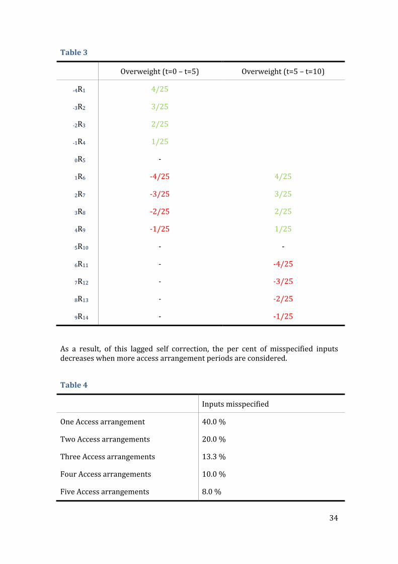
However, it should be noted that the inputs that were under-weighted in the first access arrangement are now over-weighted with the exact weightings. This is how the natural hedge works. By setting the cost of debt for the access arrangement based on the first year portfolio of debt, the inputs that are under-weighted are then over-weighted in the next access arrangement resulting in a lagged self correction. The self correcting mechanism works to an extent like an over and under mechanism between access arrangement periods. As a result, the portfolio approach with no annual adjustment is a good proxy over the long term for the version of the approach with annual adjustments.

34

Table 3

Overweight (t=0 – t=5) Overweight (t=5 – t=10)

-4R1 4/25

-3R2 3/25

-2R3 2/25

-1R4 1/25

0R5 -

1R6 -4/25 4/25

2R7 -3/25 3/25

3R8 -2/25 2/25

4R9 -1/25 1/25

5R10 - -

6R11 - -4/25

7R12 - -3/25

8R13 - -2/25

9R14 - -1/25

As a result, of this lagged self correction, the per cent of misspecified inputs decreases when more access arrangement periods are considered.

Table 4

Inputs misspecified

One Access arrangement 40.0 %

Two Access arrangements 20.0 %

Three Access arrangements 13.3 %

Four Access arrangements 10.0 %

Five Access arrangements 8.0 %

35

It should be noted that the self correcting mechanism ignores the time value of money and only works under strict conditions such as:

The benchmark term to maturity is a whole number multiple of years of the access arrangement. That is, with a 5-year access arrangement period, the benchmark term to maturity would have to be 5, 10, 15 etc.

Where the business actually issues a constant amount of debt every year which is equal to: 1 / (term to maturity).

The regulated businesses capital base is constant over time.

These conditions are unlikely to be satisfied by any regulated business. However, this does not mean that the lagged self correction mechanism does not exist. It just means it is somewhat weaker than would be the case if all of the above conditions were satisfied. To the extent self correction mechanism do not account for under- or over-weighting, the estimate is not biased.

It should be noted the benefits of the annual adjustment also decreases with the benchmark term of debt. As outlined above, when the benchmark term is five years, 40 % of the input parameters are not known at the start of the access arrangement. However, when the benchmark term of debt is ten years, only 20 % of the input parameters are unknown at the start of the access arrangement. Therefore if the benchmark term of debt is long, it questionable whether the annual adjustment is worthwhile.

A downside of the annual cost of debt adjustment is that there are costs associated with administering such annual amendments. These costs can be in terms of actual cost of estimating a benchmark, but also in terms of increased uncertainty. If annual adjustments were to be made, the regulated entity would have less certainty on what cost of debt allowance the regulator will set past the first year of the regulatory period.

For example, if a third party data provider is used to estimate the benchmark, any unanticipated change in the estimation method would result in an unforeseen change in allowed revenue. Similarly, any change in the regulator’s own method of setting the benchmark (for example due to intervention by the Australian Competition Tribunal in a non-related revenue reset appeal) could result in unexpected changes in the revenue allowance.

An important drawback of annual adjustments is that they shift the interest rate risk from the service provider to users of regulated services. However, users are in no better position to manage interest rate risk, so it is questionable why they should be exposed to it. If the interest rate risk is non-systematic it may be best if it is left with the service provider, as the shareholders of the service provider would be able to diversify this risk away by a holding a well diversified portfolio. It can therefore be argued that not adjusting the cost of debt annually strikes a better balance between consumer and business needs than if such adjustments were made.

Other disadvantages with the annual adjustment include:

36

May have an undue incentive for opportunist reviews – regulated businesses may have an added incentive to seek reviews of adjustments that result in a lowering of revenue while not challenging adjustments resulting in a revenue increase.

It increases the volatility of tariffs within the access arrangement. Users would begin the access arrangement not knowing with any certainty how much their bill will vary for the duration of the access arrangement

It increases the complexity of the annual tariff variation mechanism.

Given the above, it is recommended that the annual cost of debt adjustment should not be implemented. The cost of debt can be estimated at the start of the access arrangement based on the average cost of debt in the first year of the access arrangement with an averaging period equal to the regulated businesses benchmark term to maturity. Where possible the benchmark term of debt should be set as close to a whole number multiple of years of the access arrangement in order to ensure the self correcting mechanism has the strongest effect.

5.8. Weights within the portfolio approach

Until now it has been assumed that regulated businesses issue debt uniformly over time – i.e. they issue 20 % of their debt every year. However, regulated businesses debt issuance is likely to be lumpy over the access arrangement. For instance, if the business has large capital expenditure in the third year of the access arrangement it may have to issue an above average amount of debt in that year.

Regulated businesses have stated that the weights in the portfolio approach should reflect debt issuance assumptions in the Post Tax Revenue Model. It has been suggested that weighting new borrowings with the access arrangement at prevailing cost, will limit investment distortions, as businesses will more likely follow their capital expenditure profile assumed in the Post Tax Revenue Model.

To demonstrate what is meant by setting weights in the portfolio approach to reflect debt issuance assumptions in the Post Tax Revenue Model, consider a regulated business that has an opening regulated asset base of 1000 and has no depreciation over the access arrangement. Assume there is no capital expenditure over the access arrangement, with the exception that in year 3 when capital expenditure is equal to 1000. Further, assume the gearing ratio is 60 % and the business only issues 5 year debt and initially 20 % of the existing debt matures each year. With these assumptions the regulated business’ asset base over the access arrangement would be:

37

Table 5

TIME PERIOD 0–1 1–2 2–3 3–4 4–5

Opening asset base26 1000 1000 1000 2000 2000

Capex27 0 0 1000 0 0

Depreciation 0 0 0 0 0

Closing asset base 1000 1000 2000 2000 2000

As a result of 20 % of existing debt maturing each year and given that new capital expenditure needs to be 60 % debt financed, the regulated businesses has the following debt maturity and refinancing schedule:

Table 6

TIME PERIOD 0–1 1–2 2–3 3–4 4–5

Matured debt28 120 120 120 120 120

New borrowings29 120 120 720 120 120

Total debt30 600 600 1200 1200 1200

Given that new borrowing within the access arrangement are compensated at prevailing rate at time of the borrowing, the weight applied to the prevailing rate within the access arrangement is determined according to the following:

26 Asset base at the start of the year

27 Capital expenditure in the year.

28 Debt that has matured in the year. On average 20 % of the outstanding debt matured every year.

29 New debt that is entered into to replace matured debt and fund debt component of capex.

30 Total debt position at the end of the year. Equal to Asset base at the start of the year multiplied by 60 % minus matured debt, plus new debt, plus capex multiplied by 60 %. The assumed gearing ratio is 60 %.

38

Table 7

TIME PERIOD 0–1 1–2 2–3 3–4 4–5

Weight applied to prevailing rate31 20 % 20 % 60 % 10 % 10 %

Weight applied to existing debt rate32

80 % 80 % 40 % 90 % 90 %

As a result, the cost of debt in the first year of the access arrangement would be determined according to the following equation:

Equation 29

0TC1 =

-4R1 +

-3R2 +

-2R3 +

-1R4 +

0R5

Given the business in year 1 still issues its debt in a uniform manner, the cost of debt in year 1 is identical to how the cost of debt was determined above. However, this is not the case in year 3 of the access arrangement, where the cost of debt is determined according to the following equation:

Equation 30

2TC3 =

-2R3 +

-1R4 +

0R5

1R6 +

2R7

The cost of debt in year 4 of the access arrangement would be determined according to the following equation:

Equation 31

3TC4 =

-1R4 +

0R5

1R6 +

2R7 +

3R8

It should be noted that the prevailing rate in year 3 of the access arrangement has a largest weight applied to it due the large capital expenditure in year 3 which requires debt financing.

However, it is questionable whether weighting new borrowings within the access arrangement at the prevailing rate will achieve its main goal of

31 What proportion of total debt is refinanced in the year equal to: NEW DEBT / TOTAL

DEBT.

32 The weight applied to the last 4 years prevailing rates.

39

eliminating investment distortions. Using the earlier example where there is a large capital expenditure in year 3, regulated businesses still have an incentive to defer their capital expenditure in year 3 if the prevailing rate in year 3 is abnormally high. For instance, if the Global Financial Crisis were to occur in year 3 of the access arrangement and a business is expected to undertake a large project that requires debt financing in that year, the business may delay the investment to a time when financing can be obtained at more favourable rates. Such a practice should not be discouraged, as it is not likely to be efficient to issue debt at unfavourable times.

However, setting a large proportion of the cost of debt based on the prevailing rates in year 3 will lead to cost of the debt forecast being abnormally high for all years that year 3 cost is an input in the cost of debt under the portfolio approach. Under this scenario investment distortions will still occur and the total revenue may be set on cost of debt that is not reflective of the costs faced by the regulated business.

In order to eliminate investment distortions, a weighting scheme based on actual debt issuance data and not forecast data can be used. However, this would eliminate businesses incentives to minimise its cost of debt and will encourage businesses to issue debt at unfavourable times. Such an outcome is undesirable and would result in an inefficient cost of debt forecast.

Weighting new borrowings within the access arrangement at the prevailing cost of debt may be ineffective in preventing investment distortions within the access arrangement. Given weights are based on forecast data and not actual data, regulated business still have an incentive to delay investment if the cost of debt is abnormally high at the time of investment. The average cost of debt should be based on a simple average of the existing cost of debt. Introducing a weighting based on forecast debt issuance does not remove investment distortion but it introduces unnecessary complexity into the cost of debt forecast.

5.9. Conclusion on the portfolio approach

The cost debt over the access arrangement can be set according to the stagged debt approach with no annual adjustments, which is defined as follows:

40

Box 3

The averaging process should apply to the total cost of the benchmark debt and not just the risk-free rate. Further, a simple average should be used in the portfolio approach and not a weighted average based on debt issuance in the PTRM.

6. Estimating the benchmark

Regardless of the approach used in calculating the cost of debt, a benchmark is required to determine the cost of debt at a given point in time. Under the current approach the prevailing cost of 10-year fixed BBB+ debt must be estimated at the start of the access arrangement period. Similarly, under the portfolio approach with no annual adjustments, a benchmark cost of debt must be estimated at each averaging point in the averaging period, e.g. yearly 5-year BBB+ cost of debt over a 5-year period.

Amongst others, two key options are available to regulators when estimating the benchmark cost of debt:

Estimating own cost of debt benchmark by using individual bond yields.

Using a commercial data provider such as Bloomberg to provide a cost of debt estimate.

Regardless of the method selected, the approach needs to be predetermined in order to prevent opportunism by either the regulated businesses or the regulator. The above methods each have strengths and weaknesses that are discussed below.

6.1. Creating a new cost of debt benchmark

If it chooses to create a new benchmark for calculating the cost of debt, a regulator can select from a number of methodologies. For example, one

Equation 32

Where:




41

approach that could be implemented is to determine a simple average of the yields on bonds that have similar characteristics to the benchmark bond. Under this approach the regulator could first discover bonds that are representative of the benchmark characteristics. Once these bonds are identified, their yields can be combined in order to estimate the benchmark cost of debt.

For example, if the benchmark cost of debt is found to be a 5-year BBB+ fixed rate, the regulator may find all bonds that:

Have an outstanding maturity of 4 to 6 years

Have a credit rating of A-, BBB+ and BBB

Are fixed rate bonds

Are floating rate bonds, or are callable but have the appropriate adjustments made to them to make them equal to fixed rate equivalents

The regulator could then average the yields of these bonds to estimate the 5-year BBB+ fixed rate cost of debt. A more complex weighting scheme can also be implemented where bonds that are more reflective of the benchmark receive a higher weight than bonds that are less reflective of the benchmark (e.g. BBB+ bonds would be given more weight than either A- or BBB bonds). Regulators could also implement the ERA’s bond yield approach, which was recently endorsed by the Tribunal. However, there are some questions over the weighting scheme in that approach that requires further clarification. For example, it is unclear why an averaging scheme that places twice as much weight on a 14 year bond in contrast to a 7 year bond is appropriate or should have particular credibility.

As an alternate method for determining the cost of debt benchmark, a regulator could estimate its own yield curve through an econometric model that predicts the cost of debt based on explanatory parameters including those that describe the benchmark – such as term to maturity and credit rating. Such methods have the potential to lead to more accurate benchmark cost of debt forecasts.

The key advantage of a regulator developing its own cost of debt methodology is that it could result in greater transparency and certainty when compared with the unknown methodology used by Bloomberg in arriving at its Bloomberg Fair Value estimate. However, in estimating its own cost of debt benchmark, agreement would need to be sought over the appropriate method as well as the appropriate data.

Developing a cost of debt methodology, however, is not without shortcomings. First, it is not clear how individual bond yields should be combined to estimate the cost of debt. As noted above, a simple average can be used, but such an approach will at times lead to an inaccurate cost of debt estimate. For instance, using the above example, if the sample of bonds contains relatively more 4-year bonds and more A- rated bonds, the benchmark would likely under-estimate the 5-year BBB+ cost of debt.

On the other hand using more complex weighting or econometric models could introduce greater difficulty in estimating the cost of debt. For example, the Nelson- Siegel model involves the use of more elaborate econometric techniques.

42

The benefit of introducing such complexity may not outweigh the cost. Further, it is not certain that a regulator, in consultation with industry, can arrive at a methodology for determining the benchmark cost of debt which is, under all circumstances, superior to the current methodology. Even attempting to do so may give rise to claims of false precision.

Second, creating a new cost of debt methodology raises the issue of whether the input data is of high quality. It must be noted that if the input data in a regulator’s cost of debt methodology is of a low quality, the resulting cost of debt forecast will also be of a low quality. If the regulator were to estimate it own benchmark, the data inputs in the estimate cost of debt would have to be of a high quality to ensure the estimate reflects the actual cost of funds. To do this, the regulator would have to ensure the sample bonds are currently traded and that their yield represents current market conditions.33

Thirdly, if it estimated its own benchmark, a regulator may need to continually refine the methodology, even if the broad approach is constant, to ensure ongoing adequacy and appropriateness of the approach. For example, if data required by the methodology was no longer available, the regulator would need to alter the methodology (perhaps substantially) to compensate. This could reduce both transparency and certainty of the approach.

Estimating one’s own cost of debt benchmark is a complex task. It requires the regulator to determine a methodology and ensure the inputs parameters are of a high quality. As outlined above, there are many possible variations of the cost of debt estimation methodology and it is unlikely that any given method can be considered to be the best. Consequently, creating a “state of the art” cost of debt methodology can lead to a false sense of precision. Even if agreed to initially, it is possible that at some point in the future this precision will be questioned. Any gain in precision (if existent) would need to be weighed against the appropriateness of the approach against alternatives.

6.2. Using a commercial data provider

Instead of estimating its own benchmark, a regulator can use a commercial data service provider’s yield curve to estimate the cost of debt at a particular point in time. For example, consistent with the current practice of some regulators, one could estimate the cost of debt benchmark using the Bloomberg Fair Value curve.

A key benefit associated with using the Bloomberg Fair Value curve is that it is produced by a commercial organisation that is independent of parties to a regulatory process. However, problems may arise if Bloomberg does not offer a suitable benchmark. For example, if a regulator is to adopt a 10-year benchmark, Bloomberg Fair Value curve does not extend to that term for BBB credit rating, so appropriate extrapolation methods would need to be developed to extend the longest Bloomberg yield (7 years for BBB) to the 10-year horizon. The Tribunal

33 The yield data of bonds that are not traded may be outdated and as a result the yields are

not reflective of the current market conditions. It has to be noted that the most information about bond pricing is available on the day of issue (primary market). Once the bonds are traded in the secondary market, they will not be priced if they are not traded.

43

has also acknowledged “there appears to be increasing doubt as to its reliability”.34

Further, the Bloomberg Fair Value curve is not specific to the benchmark firm. There is no BBB+ specific Bloomberg Fair Value curve, as Bloomberg only provides a generic BBB band curve.35 The “representative” bonds Bloomberg uses could be biased towards a credit rating above or below the credit rating of the debt proxy. Further, the Bloomberg Fair Value curve represents the lending costs faced by all business within a rating band and not necessarily reflects the lending costs faced by regulated businesses.

As outlined in section 3.3, when contrasted to the actual debt issuance costs of regulated businesses, following the Global Financial Crisis the Bloomberg Fair Value curve has provided an abnormally high cost of debt. This led some regulators such as the AER to attempt to move away from solely relying on the Bloomberg estimate. Further, relying on the Bloomberg Fair Value as the method of estimating the benchmark cost of debt will become unsustainable if Bloomberg decided to cease publishing its fair value curve in the future. A similar situation occurred in the past when the Commonwealth Bank ceased publishing the CBA Spectrum yield estimate which was previously relied on (at least in part) in cost of debt estimation.36

However, the issue of the Bloomberg Fair Value over or under-estimating the regulated business cost of debt becomes less problematic when the cost of debt is estimated using a portfolio approach with no annual adjustments. This is because the approach estimates the cost of debt as an average of a number of Bloomberg Fair Value estimates. The process of averaging may result in periods were the Bloomberg Fair Value over-estimates the cost of debt being somewhat offset by periods where the Bloomberg Fair Value under-estimates the cost of debt.37 Figure 13 shows that under the current, point estimate, approach the BFV over or under-estimates the cost of debt at any given point in time by sometimes a significant amount.38 This is a major concern if the cost of debt is estimated at a point where BFV diverges from actual bond yields.

34 Australian Competition Tribunal, Application by WA Gas Networks Pty Ltd (No 3) [2012]

ACompT 12, p. 44.

35 The combined credit rating of BBB-, BBB and BBB+.

36 In the past the AER had to weight up the benefits of two benchmarks (CBA Spectrum and the Bloomberg Fair Value). However, the Commonwealth Bank decided to cease publishing the CBA spectrum due to its unreliability. This resulted in the AER only having one independent data provider.

37 Assuming there is no systematic over-estimation in the Bloomberg Fair Value.

38 This is based on the assumption that the average bond yields produce the correct estimate of the 5 year cost of debt.

44

Figure 13: (BBB 5 year BFV) minus (average yield on bonds with maturity of 3 to 7 years and BBB band credit rating).

However, as outlined in Figure 14 using an average in the portfolio approach, results in periods of over estimation being offset by periods of under estimation. As is evident the bias in using the Bloomberg Fair Value is within 50 basis points of bond yields with similar characteristics. If the benchmark term of debt is more than 5 years; the process of averaging will further eliminate any divergence.

Figure 14: (5 year annual average BBB 5 year Bloomberg Fair Value) minus (5 year annual average of the average yield on bonds with maturity of 3 to 7 years and BBB band credit rating).

Due to the averaging process in the portfolio approach, the issue with the Bloomberg Fair Value over or under-estimating regulated businesses cost of debt is less problematic than was the case under the point estimate cost of debt method.

45

However, a key disadvantage of the use of a Bloomberg estimate is that there is no certainty that the Bloomberg Fair Value estimates will continue to be published. In that case, it may be impossible to provide a consistent estimate of the benchmark cost of debt through time, and across various decisions. These problems are exacerbated under the portfolio approach, which requires a number of estimates to be used at different points in time. Similar issues could arise if Bloomberg chooses to vary its method of estimating the fair value curve.

If regulators were to continue using the Bloomberg Fair Value curve, ongoing periodic assessment of the curve relative to the observed yields in the market should be made.

6.3. Conclusion on estimating the benchmark

A regulator has two broad alternatives in deciding as to how to estimate the cost of debt benchmark at particular point in time. It can create its own benchmark cost of debt or continue to the use the Bloomberg Fair Value curve. Each of the methods has its own strengths and weaknesses.

If the regulator chose to create its own cost of debt methodology it would need to undertake a complex task, which may expose it to potential errors and could require significant exercise of judgement. Given many potential methodologies for estimating the cost of debt, it may never be clear which approach will result in the most accurate estimate. As a result, a regulator creating the its own cost of debt methodology can lead to a false sense of precision even while increasing transparency.

On the other hand, using the Bloomberg Fair Value effectively outsources the cost of debt determination to Bloomberg. While it may be seen to relinquish some of the control over estimating the cost of debt at a particular point, this method protects the regulator from having to defend its approach against many other possible options, any one of which could be seen as superior at a particular point in time and inferior at another. Further, given the recommendation that regulators implement a portfolio approach with no annual adjustment, which averages cost of debt over time, problems caused by the Bloomberg Fair Value estimate over or under-compensating the regulated business are diminished.

It is argued here that each method has its own advantages and disadvantages. It is open to regulators to determine which method is most appropriate and fit for purpose.

7. Transitional arrangements

Should a regulator choose the portfolio approach, it would be appropriate to set out transitional arrangements from the current prevailing cost of debt approach. The transitional arrangements would be used for all future access arrangements, including first access arrangements of any new regulated firms. This is because the portfolio debt approach assumes the firm has a pre-existing debt exposure which is not the case for a new firm.

Under the current prevailing cost method, regulated businesses are expected to refinance all of their debt at the start of the access arrangement with 10-year rate debt. At the end of the access arrangement, under this method regulated

46

businesses are expected to again refinance all of their debt with 10-year debt, even though the businesses existing debt is only half way to maturity (five years into the 10-year debt). Regulated businesses are also not compensated for the cost of expiring debt prematurely under the prevailing cost of debt methods (see limitation of the current method discussed in section 3.1).

These issues, however, would not be present if businesses are assumed to issue debt equalling the regulatory period of 5 years. Assuming they issue 5-year debt, and issue a total of five bonds, the regulated businesses are expected to have the following debt exposure:

Figure 15

The 5-year cost of debt line only runs for 5 years as the businesses is assumed, under the prevailing cost method, to refinance all of its debt at the end of the access arrangement.

However, under the portfolio approach with no annual adjustments regulated businesses are expected to refinance 1/nth of their portfolio every year with n-year term debt, where n is the benchmark term of debt. If the average term is equal to 5 years, the approach assumes the regulated businesses to have the following debt exposure:

Figure 16

47

Transitional arrangement should be introduced for all of firm’s cost of debt in order to ensure the regulated business and consumers are not adversely affected by the change in methodology. This is because the portfolio approach assumes businesses have entered into debt positions in the past. For example, at the start of the access arrangement the approach with a 5-year cost of debt assumption supposes regulated business have a 20 % exposure to 5-year debt that was entered into one, two, three and four years prior to the commencement of the access arrangement.

However, regulated business may not have these exposures at the start of the first access arrangement when the new approach is introduced, as its actual debt issuance may be geared towards reflecting the previous regime. Instead, regulated businesses may still hold 5-year bonds issued during the previous access arrangement.

One method to transition the revenue allowance calculation from a prevailing cost approach to a portfolio of debt approach is to use short term debt as filler between the two methods. For example, under a 5-year term assumption, the cost of debt for the transitional access arrangement can be determined as 20 % each from 1-year to 5-year fixed rate debt.

When the initial debt exposures expire, the business would then roll over its exposure to new 5-year debt – e.g. one year into the new access arrangement, the assumed 1-year bond expires and new 5-year debt is entered into. The transitional arrangement can be represent graphically as follows, where the red represents the prevailing cost approach, blue represents the transitional arrangement and green represent the transitioned portfolio approach with non annual adjustments:

Figure 17

A similar approach can be adopted for transitioning from a 10-year prevailing cost of debt method to the portfolio approach.

48

Transitional arrangements should not be provided when a business is sold to another party. Despite the change in ownership, the businesses should be considered as an ongoing concern with one owner over the entire life of the asset.39

8. A worked example

As outlined earlier, the cost of debt over the access arrangement could be estimated in accordance approach with no annual adjustments as defined by the following:

Equation 33

To demonstrate how the portfolio approach with no annual adjustments can work in practice, assume a regulator wants to estimate the cost of debt of a regulated business for a 5-year access arrangement commencing on the 1 July 2012. Assume that the benchmark term of debt is equal to 10 years with a credit rating of BBB and is estimated using the Bloomberg Far Value estimate. As a result the above formula becomes as follows:

Equation 34

The cost of debt data is sourced from 10-year BBB Bloomberg Fair Value,40 resulting in the following input parameters:

39 A new asset owner would not have any pre existing debt at the time it purchases the

asset. Therefore if the prevailing cost of debt at time of the purchase is higher than the portfolio cost of debt, the new asset owner maybe disadvantaged. Due to this disadvantage, the new asset owner would pay less for the asset, than what would have been the case if transitional arrangement had been in place. So the new asset owner would not be worse off as it just pays less to acquire the asset. The investor that sells the asset will also not be worst off, because smaller amount it receives on the asset sale is offset by the gain it received from prematurely closing out its debt portfolio. I.e. there is no net loss in this situation, and no transitional arrangements should be warranted.

40 Note the 10-year BBB Bloomberg Fair Value currently does not exist and as a result the 10 year BBB Bloomberg Fair Value must be estimated through the use of extrapolation methods.

49

Table 8

Input Parameter BFV date BFV Value

1 July 2003 6.40

1 July 2004 7.11

1 July 2005 6.16

3 July 2006 6.78

2 July 2007 7.49

1 July 2008 9.38

1 July 2009 8.70

1 July 2010 9.41

1 July 2011 9.56

2 July 2012 6.67

Inserting the Bloomberg Fair Value estimates into the formula, determines the cost of debt estimate over for the 2012-2017 access arrangement period for the regulated business.

Equation 35

=

= 7.77 %

As a result, the regulated business would receive a 7.77 % cost of debt allowance over the 2012-2017 access arrangement. It should be noted that this cost of debt example ignores transitional arrangements.

9. Other forms of financing

Under many current regulatory regimes regulators determine the cost of debt based only on Australian fixed-rate term of debt. However, Moody’s Investors Service presented data showing that in each year between 2009 to 2011 domestic capital markets accounted for around one-third of issuance by regulated energy network service providers, with the bank market and offshore

50

markets providing the remaining two thirds.41 Therefore many regulators currently do not take account of two thirds of the financing cost faced by regulated business. These regulators usually have no regard to other forms of financing such as:

Banks financing

Floating rate bonds

International bonds

Callable

Subordinate

Further, many regulators currently have no regard to the changes in efficient mix of types of financing over time. For example, while only fixed debt is used in determining a benchmark, at a given point of time issuing fixed rate debt may not be the most efficient method of sourcing debt financing. Further, even if fixed debt is efficient, debt of assumed tenor may not be. For example, during the Global Financial Crisis issuing 10-year debt was not only inefficient, but also nearly impossible to achieve and only shorter term debt was issued.

Regulated businesses do issue other forms of financing and do not limit their lending to the current benchmark of fixed rate 10-year BBB+ debt in Australia. Sometimes the other forms of financing can be converted into Australian Fixed rate equivalents42 using derivatives, while other forms of financing cannot be converted to Australian fixed rate equivalent debt.

Over time regulated businesses adopt a dynamic approach to debt financing while a static approach is assumed by regulators. At any given point in time, a regulated business would be expected to weigh up the cost of all alternative sources of financing and select the financing option(s) that results in the lowest expected cost.

For example, prior to the Global Financial Crisis regulated businesses used credit wrapping extensively, as this process resulted in lowest cost of debt. However, the ability to use credit wrapping disappeared as a result of the Global Financial Crisis. In addition, during the Global Financial Crisis regulated business primarily obtained bank financing or short term bond financing as the long term corporate bond market became illiquid. While these changes in debt sourcing occurred, in both pre, during and post-Global Financial Crisis periods, regulators often based their cost of debt benchmark on Australian 10-year fixed rate corporate bonds yields. However, during the Global Financial Crisis it is unlikely regulated businesses were issuing (or were able to efficiently issue) debt with these benchmark characteristics.

Restricting a regulator’s determination of the cost of debt benchmark on one source of funds (Australian fixed rate corporate bonds) ignores the financing

41 Australian Regulated Electricity and Gas Network Outlook 2012.

42 For instance, floating rate bonds are converted to fixed rate equivalents by using interest swap. Also foreign bonds are converted into Australian fixed rate equivalents using currency swaps.

51

options the regulated businesses has and as result will over compensate the regulated business for its cost of debt.

To illustrate this graphically, assume there is two source of financing (Financing Option 1 and Financing Option 2) and they are perfectly negatively correlated.

Figure 18

If the regulator were to base its cost of debt forecast on only Financing Option 1, the average allowed cost of debt would be:

52

Figure 19

However, if the regulated business optimally selects the cheapest source of debt financing over time, the actual average cost of debt faced by the regulated business is below the average cost of debt approved by the regulator:

Figure 20

It should be noted that the above example does not reflect what actual happens in reality. Different sources of financing are not perfectly negatively correlated

53

and arbitrage opportunities limit the difference in yields between alternative sources of debt finance. However, the example does highlight that regulated business have a choice when it comes to debt financing. They can select different sources (bank debt, fixed, floating, international, callable, subordinate etc) and can also issue different maturities (e.g. issuing short term debt when the cost of debt is high and long term debt when the cost of debt is low). However, given the options available to the regulated business, a regulator adopting a static approach (one source of financing, based on static parameters: e.g. 10-year term Australian fixed debt) will lead to the regulated business being over compensated on average.

In an ideal world, a regulator would estimate what proportion of funds will be allocated to each source of debt financing and have the cost of debt allowance account for all sources of finance. However, this may be difficult to do as it is only possible to know what financing option is efficient at the time when the financing needs to be raised. It may not be known at the start of the access arrangement. Further, data on alternative sources is not always available, and if available it is not always in a useable format.

Given the regulator cannot calculate the cost of debt by applying an appropriate weight to each source of debt financing, the second best method is to compensate the regulated business with reference to one source of debt financing. However it should be explicitly recognised in decisions that such a method over time will result in a conservative cost of debt estimate favouring the regulated business.

10. The averaging period over which the cost of debt should be estimated

Under the prevailing cost method, the averaging period is very important. Regulated businesses are required to choose an averaging period between 5 to 40 days immediately prior to the beginning of the new access arrangement period over which to estimate their cost of debt and the risk free rate. The businesses have the choice in advance of the averaging period, and this period is theoretically used by businesses to enter swap transactions in order to hedge their interest rate exposure.

Unlike the prevailing cost method which has one averaging period, the portfolio approach with no annual adjustments has multiple averaging periods. For instance, with a five year benchmark term of debt assumption and annual refinance frequency, there are five averaging periods. It should be noted at the time of the access arrangement review, at least 4 of these averaging periods have occurred in the past. As a result, the businesses should not have a choice of these past averaging periods.

If the businesses are provided with a choice for the past averaging periods, they will select the averaging period that gives them the highest revenue and not the averaging period which more accurately reflects their debt issuance practices. Consequently, for the portfolio approach with no annual adjustments, the averaging period should be determined either by:

The regulator

54

The regulated business, except the regulated businesses selects the averaging period that will apply in the next 5 years and not the averaging period that applied for the last 5 years.

Either method is acceptable, however no method should be endorsed that allows a regulated business to have choice of an averaging period that has already occurred. The benefit of the regulated business selecting the averaging period is that they will select an averaging period that is likely to be independent of other regulated businesses averaging periods. This is desirable to ensure all regulated business are not forced to enter the swap/debt markets at the same time, as that could result in unfavourable swap rates stemming from the increased demand.

Further, as outlined in Section 5 the portfolio approach requires the cost of debt to be estimated at the start of access arrangement. However, the final regulatory decisions are completed at least 3 months prior to the commencement of the access arrangement. As a result, assuming a 5-year benchmark term of debt is used, the averaging periods for the cost of debt could either be:

Brought forward three months for all cost of debt inputs.

Estimated in line with the commencement of the access arrangement. In this situation at the time of the final decision an estimate could be made of the 5-year cost of debt in three months time. This estimate would then be updated at the start of the next access arrangement. This process is similar to how final-year capex is updated for the difference between estimates and actual expenditure.

Under both options business can engage in debt issuance strategies that minimise their risk exposure. However, bringing averaging periods forward by three months is preferable as it removes the transactions costs associated with updating the cost of debt at the start of the next access arrangement.

11. Conclusion

This paper develops a new methodology for estimating the cost of debt for a regulated business over the access arrangement. The new cost of debt methodology is a response to the shortcoming of the current cost of debt approach and the advice provided by the Tribunal.

It is argued that the cost of debt over the access arrangement can be determined according to the portfolio approach with no annual adjustments, which can be estimated as:

55

Box 4

If this approach is implemented, it is argued that regulated businesses should not be provided with a choice of method of cost of debt estimation. Providing choices to regulated businesses will result in regulated businesses selecting the option that leads to highest revenue and not the option that represents efficient debt financing, and may result in multiple benchmarks, adversely affecting the firm’s incentive to act efficiently.

This paper has not taken a strong view on whether the benchmark cost of debt should be estimated using a commercial data provider, or whether regulators should estimate their own yield curve. This is because each method has its own advantages and disadvantages and it up to regulators to determine which benchmark cost of debt method is most appropriate.

Equation 36

Where:




Estimating the Cost of Debt - Australian Competition and ... Development... · Current regulatory...

Documents

Transcript of Estimating the Cost of Debt - Australian Competition and ... Development... · Current regulatory...