Estimating Term Structure withPenalized Splines

David Ruppert

Operations Research and Industrial Engineering

Cornell University

Joint work with Robert Jarrow and Yan Yu

January 27, 2004

1

Outline

• Bond prices, forward rates, yields

• Empirical forward rate – noisy

• Modelling the forward rate

• Penalized least-squares

• Inadequacy of cross-validation

• Residual analysis – checking the noise assumptions

• Corporate term structure and credit spreads

• Asymptotics

2

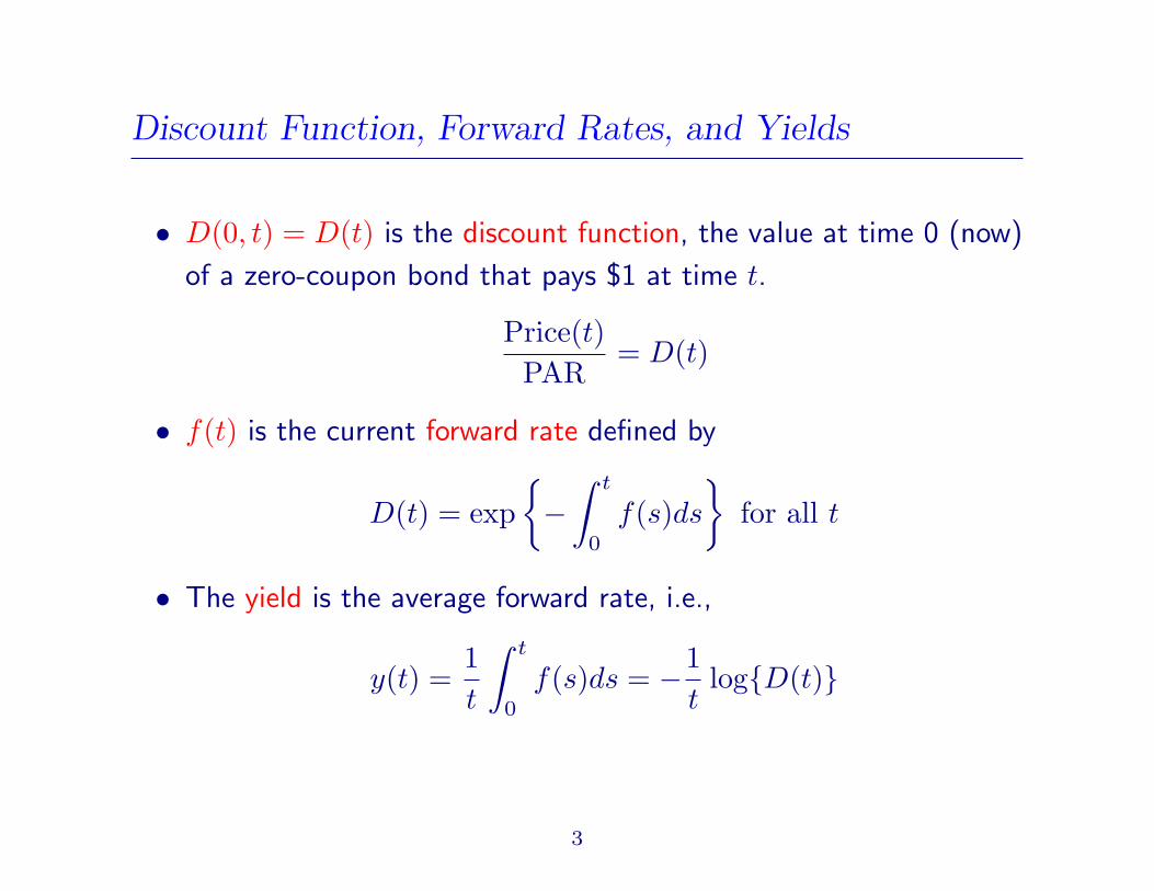
Discount Function, Forward Rates, and Yields

• D(0, t) = D(t) is the discount function, the value at time 0 (now)

of a zero-coupon bond that pays $1 at time t.

Price(t)PAR

= D(t)

• f(t) is the current forward rate defined by

D(t) = exp−

∫ t

0

f(s)ds

for all t

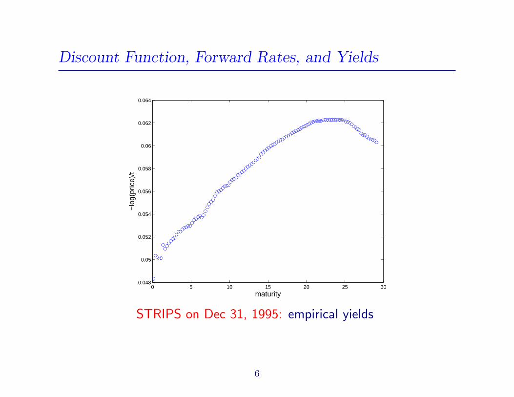
• The yield is the average forward rate, i.e.,

y(t) =1t

∫ t

0

f(s)ds = −1t

logD(t)

3

Discount Function, Forward Rates, and Yields

0 5 10 15 20 25 300.1

0.2

0.3

0.4

0.5

0.6

0.7

0.8

0.9

1

pric

e

maturity

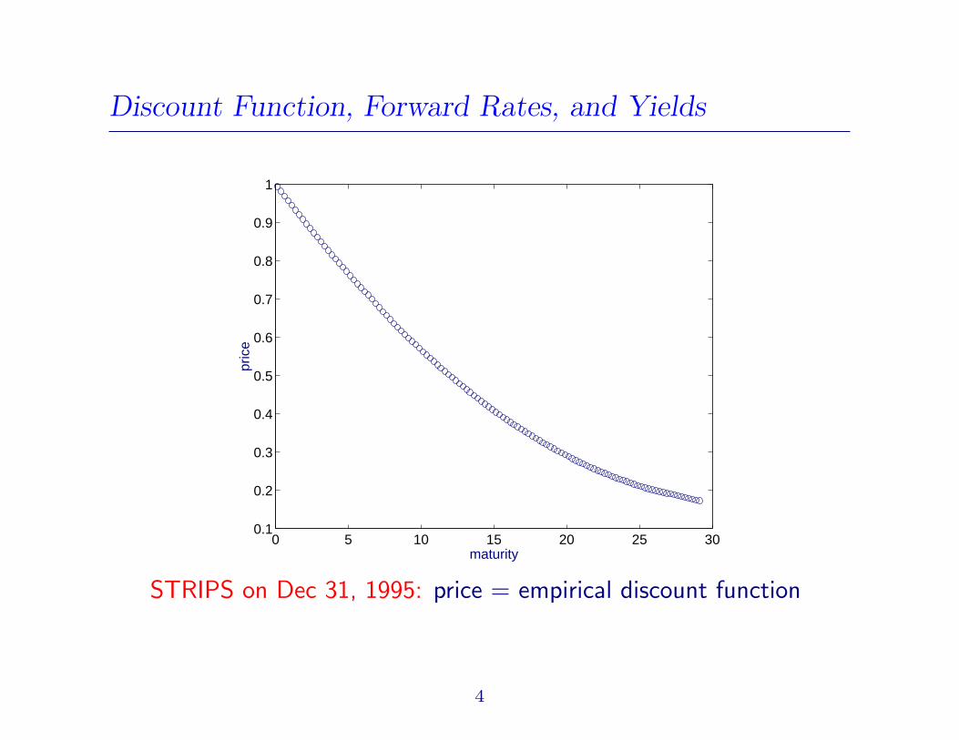
STRIPS on Dec 31, 1995: price = empirical discount function

4

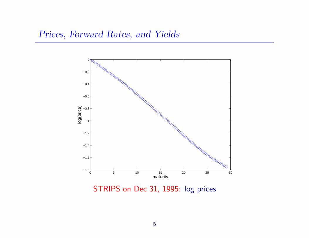
Prices, Forward Rates, and Yields

0 5 10 15 20 25 30−1.8

−1.6

−1.4

−1.2

−1

−0.8

−0.6

−0.4

−0.2

0

maturity

log(

pric

e)

STRIPS on Dec 31, 1995: log prices

5

Discount Function, Forward Rates, and Yields

0 5 10 15 20 25 300.048

0.05

0.052

0.054

0.056

0.058

0.06

0.062

0.064

maturity

−lo

g(pr

ice)

/t

STRIPS on Dec 31, 1995: empirical yields

6

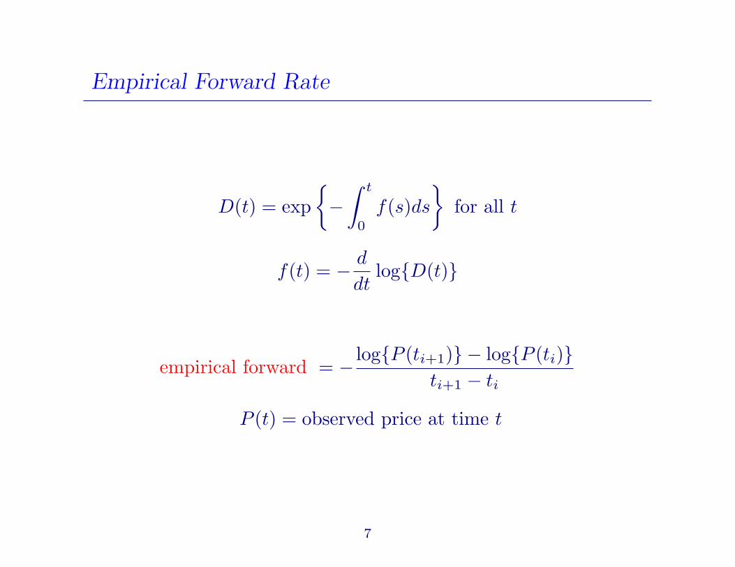
Empirical Forward Rate

D(t) = exp−

∫ t

0

f(s)ds

for all t

f(t) = − d

dtlogD(t)

empirical forward = − logP (ti+1) − logP (ti)ti+1 − ti

P (t) = observed price at time t

7

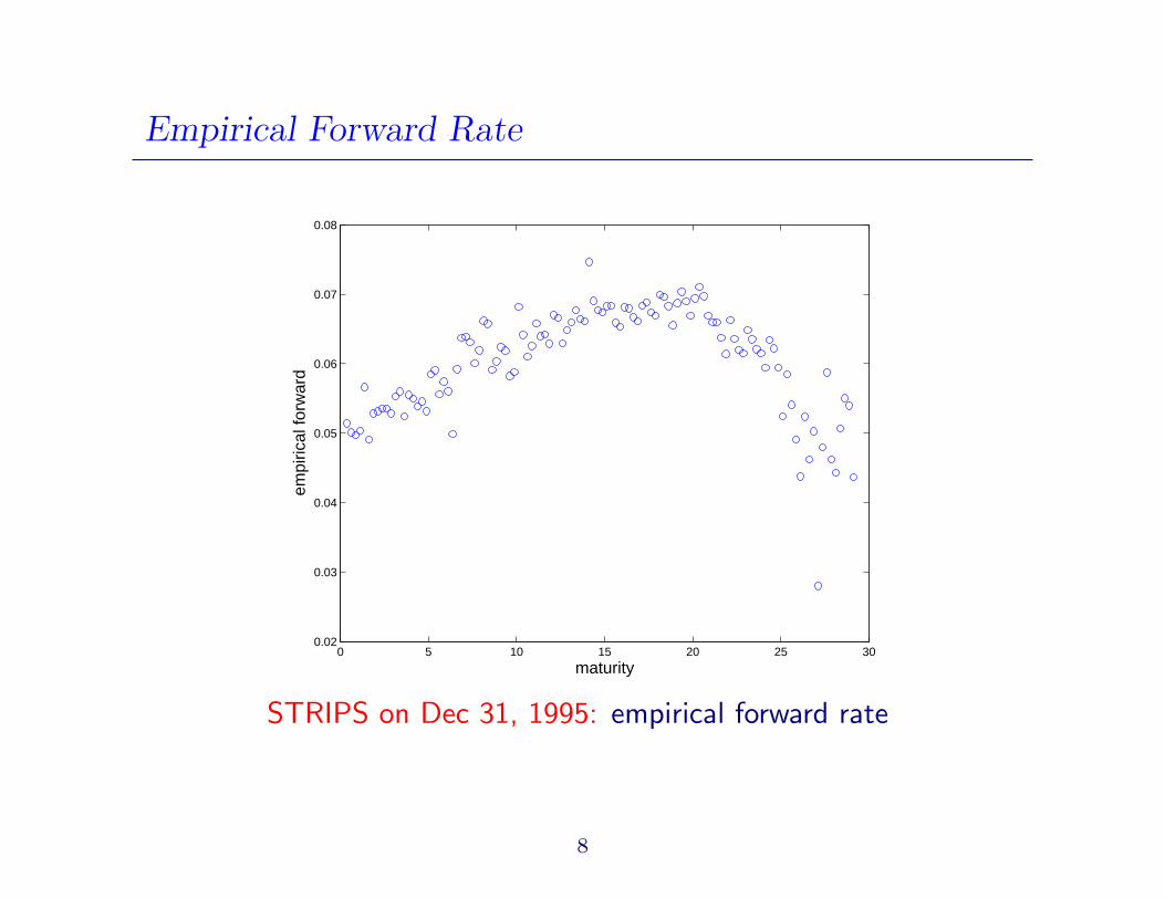
Empirical Forward Rate

0 5 10 15 20 25 300.02

0.03

0.04

0.05

0.06

0.07

0.08

maturity

empi

rical

forw

ard

STRIPS on Dec 31, 1995: empirical forward rate

8

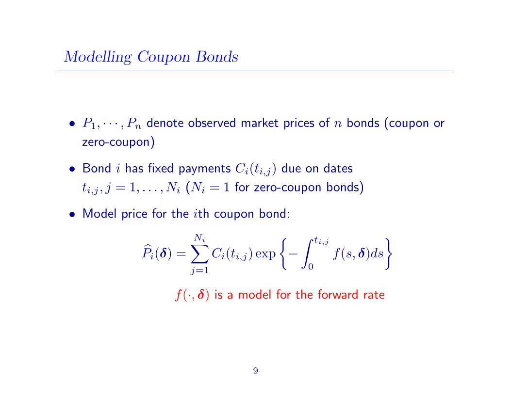
Modelling Coupon Bonds

• P1, · · · , Pn denote observed market prices of n bonds (coupon or

zero-coupon)

• Bond i has fixed payments Ci(ti,j) due on dates

ti,j , j = 1, . . . , Ni (Ni = 1 for zero-coupon bonds)

• Model price for the ith coupon bond:

Pi(δ) =Ni∑

j=1

Ci(ti,j) exp−

∫ ti,j

0

f(s, δ)ds

f(·, δ) is a model for the forward rate

9

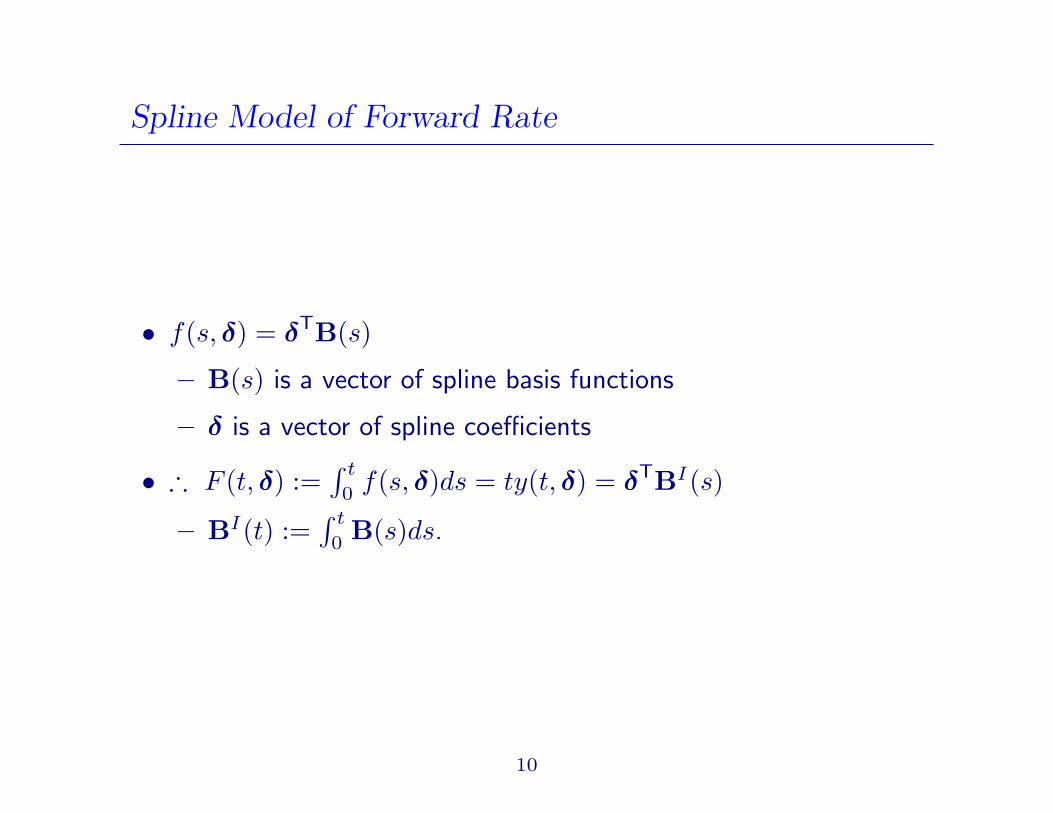
Spline Model of Forward Rate

• f(s, δ) = δTB(s)

– B(s) is a vector of spline basis functions

– δ is a vector of spline coefficients

• ∴ F (t, δ) :=∫ t

0f(s, δ)ds = ty(t, δ) = δTBI(s)

– BI(t) :=∫ t

0B(s)ds.

10

Example: Quadratic Splines

B(s) =(1, s, s2, (s− κ1)2+, . . . , (s− κK)2+

)T

0.0 0.2 0.4 0.6 0.8 1.0

-0.0

50.

00.

050.

100.

15

Plus function with knot at 0.6

11

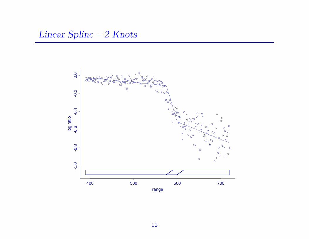
Linear Spline – 2 Knots

range

log

ratio

400 500 600 700

-1.0

-0.8

-0.6

-0.4

-0.2

0.0

12

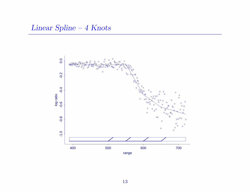
Linear Spline – 4 Knots

range

log

ratio

400 500 600 700

-1.0

-0.8

-0.6

-0.4

-0.2

0.0

13

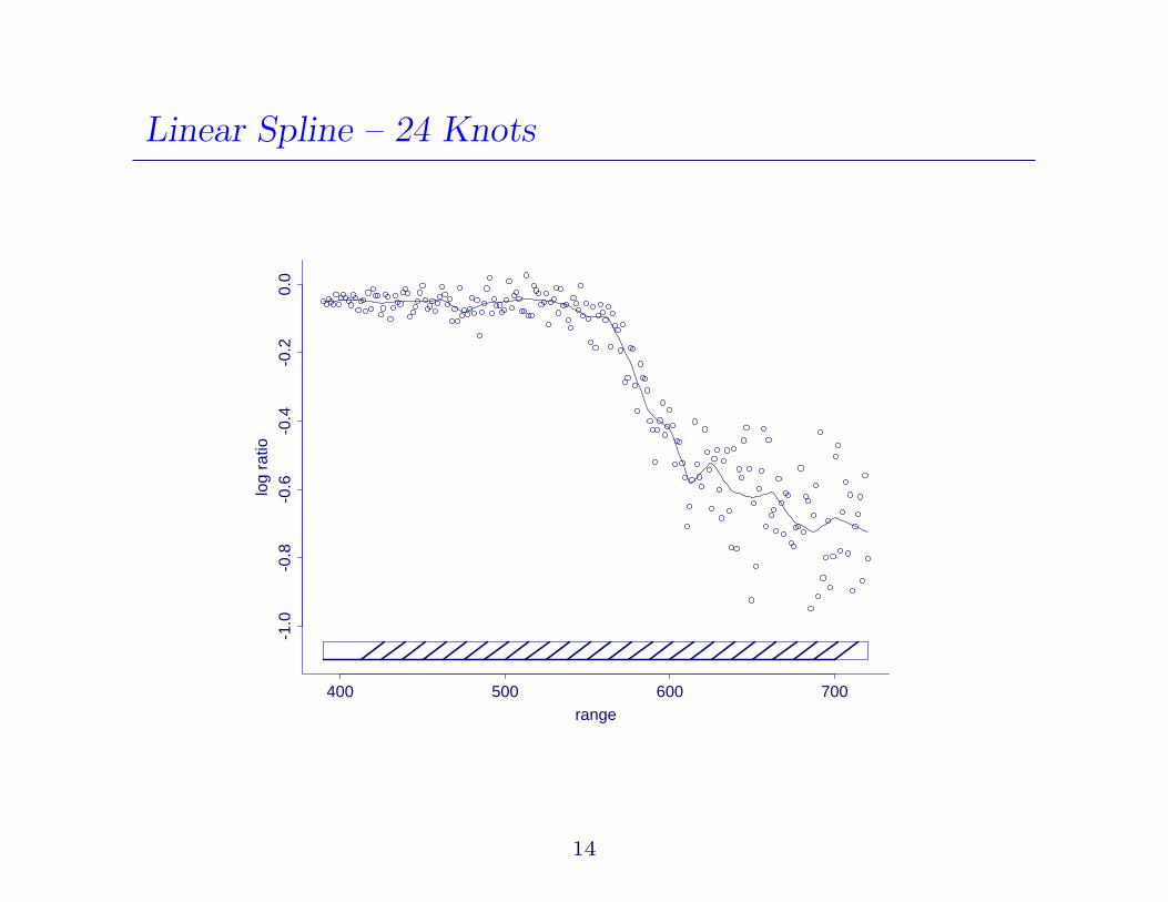
Linear Spline – 24 Knots

range

log

ratio

400 500 600 700

-1.0

-0.8

-0.6

-0.4

-0.2

0.0

14

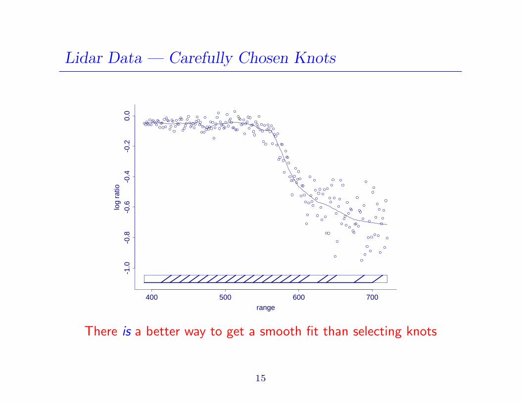
Lidar Data — Carefully Chosen Knots

range

log

ratio

400 500 600 700

-1.0

-0.8

-0.6

-0.4

-0.2

0.0

There is a better way to get a smooth fit than selecting knots

15

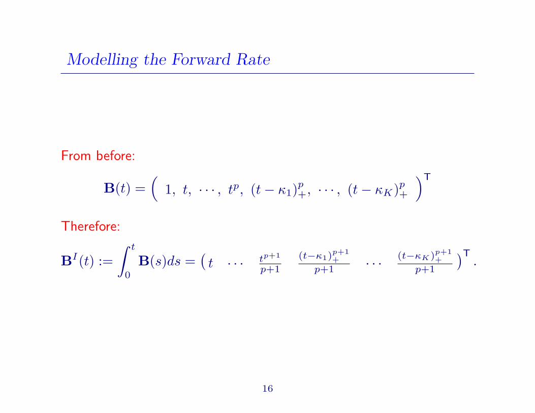
Modelling the Forward Rate

From before:

B(t) =(

1, t, · · · , tp, (t− κ1)p+, · · · , (t− κK)p

+

)T

Therefore:

BI(t) :=∫ t

0

B(s)ds =(t · · · tp+1

p+1

(t−κ1)p+1+

p+1 · · · (t−κK)p+1+

p+1

)T.

16

Penalized Least-Squares

Qn,λ(δ) =1n

n∑

i=1

[h(Pi)− hPi(δ)

]2

+ λδTGδ

or equivalently

Qn,λ() =1

n

nXi=1

(h(Pi)− h

"NiXj=1

Ci (ti,j) expn−TBI(ti,j)

o#)2

+λTG.

• h is a monotonic transformation: “transform-both-sides” model

• λδTGδ is a “roughness” penalty

– λ ≥ 0

– G is positive semi-definite

17

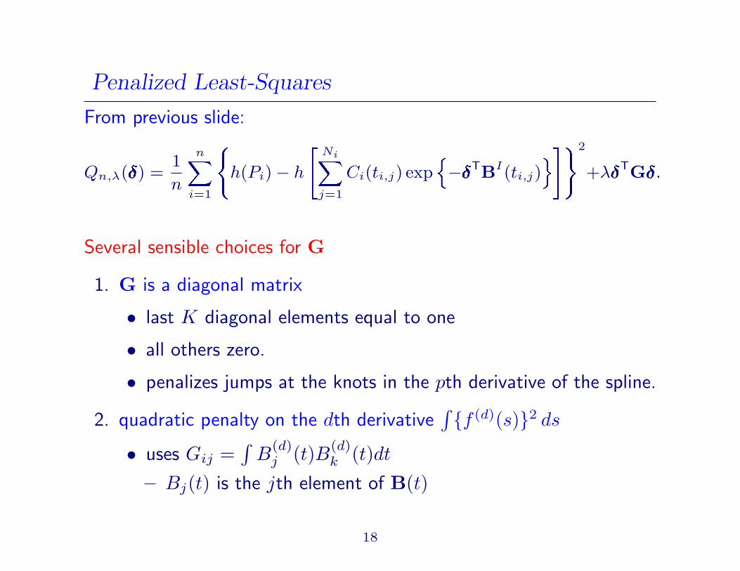
Penalized Least-Squares

From previous slide:

Qn,λ() =1

n

nXi=1

(h(Pi)− h

"NiXj=1

Ci(ti,j) expn−TBI(ti,j)

o#)2

+λTG.

Several sensible choices for G

1. G is a diagonal matrix

• last K diagonal elements equal to one

• all others zero.

• penalizes jumps at the knots in the pth derivative of the spline.

2. quadratic penalty on the dth derivative∫ f (d)(s)2 ds

• uses Gij =∫

B(d)j (t)B(d)

k (t)dt

– Bj(t) is the jth element of B(t)

18

Linear Spline with 24 Knots Fit by Penalized LeastSquares

range

log

ratio

400 500 600 700

-1.0

-0.8

-0.6

-0.4

-0.2

0.0

• Number of knots has little effect on fit provide it is at least 15

• Choice of λ is crucial

19

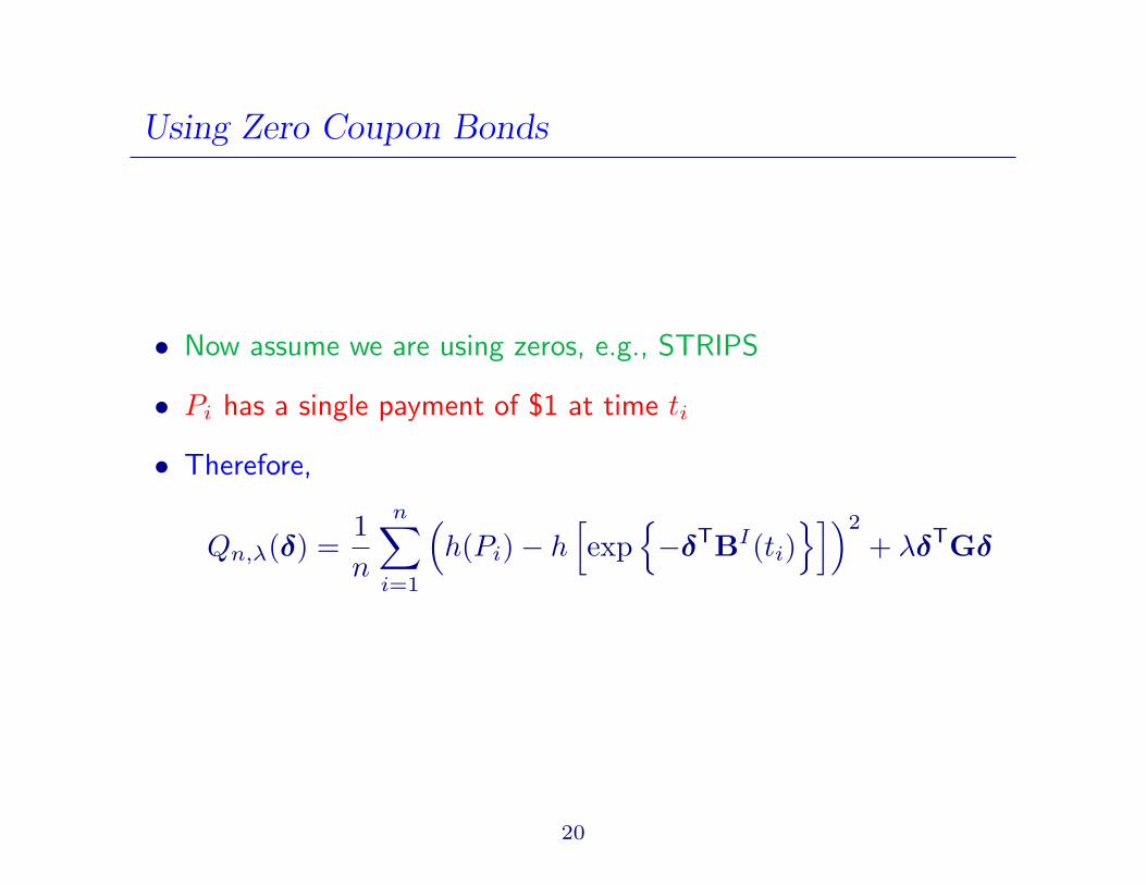
Using Zero Coupon Bonds

• Now assume we are using zeros, e.g., STRIPS

• Pi has a single payment of $1 at time ti

• Therefore,

Qn,λ(δ) =1n

n∑

i=1

(h(Pi)− h

[exp

−δTBI(ti)

])2

+ λδTGδ

20

Choosing the Knots

• κk is the k(K+1) th sample quantile of tin

i=1

• the ti are nearly equally spaced so the knots are also

21

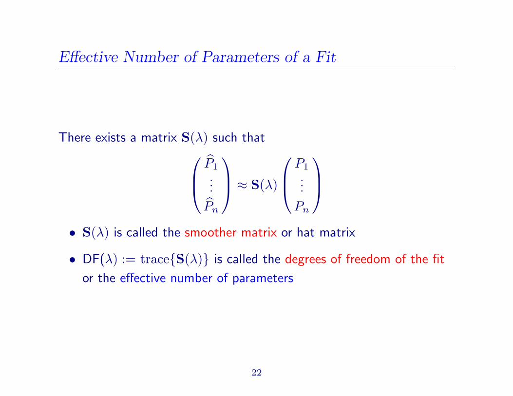
Effective Number of Parameters of a Fit

There exists a matrix S(λ) such that

P1...

Pn

≈ S(λ)

P1...

Pn

• S(λ) is called the smoother matrix or hat matrix

• DF(λ) := traceS(λ) is called the degrees of freedom of the fit

or the effective number of parameters

22

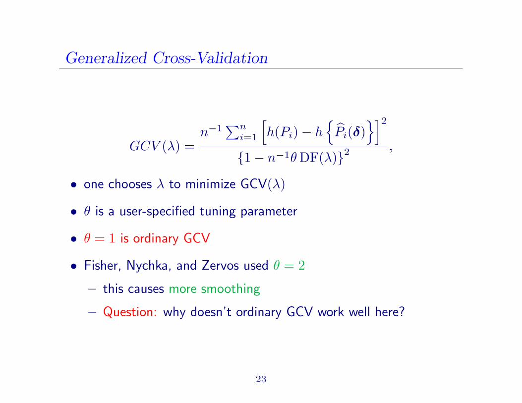
Generalized Cross-Validation

GCV (λ) =n−1

∑ni=1

[h(Pi)− h

Pi(δ)

]2

1− n−1θ DF(λ)2 ,

• one chooses λ to minimize GCV(λ)

• θ is a user-specified tuning parameter

• θ = 1 is ordinary GCV

• Fisher, Nychka, and Zervos used θ = 2

– this causes more smoothing

– Question: why doesn’t ordinary GCV work well here?

23

EBBS

• To estimate MSE add together:

– estimated squared bias

– estimated variance

• Gives MSE(f ; t, λ), the estimated MSE of f at t and λ.

– then∑n

i=1 MSE(f ; ti, λ) is minimized over λ

• EBBS estimates bias at any fixed t by

– computing the fit at t for a range of values of the smoothing

parameter

– fitting a curve to model bias

24

EBBS – Estimating Bias

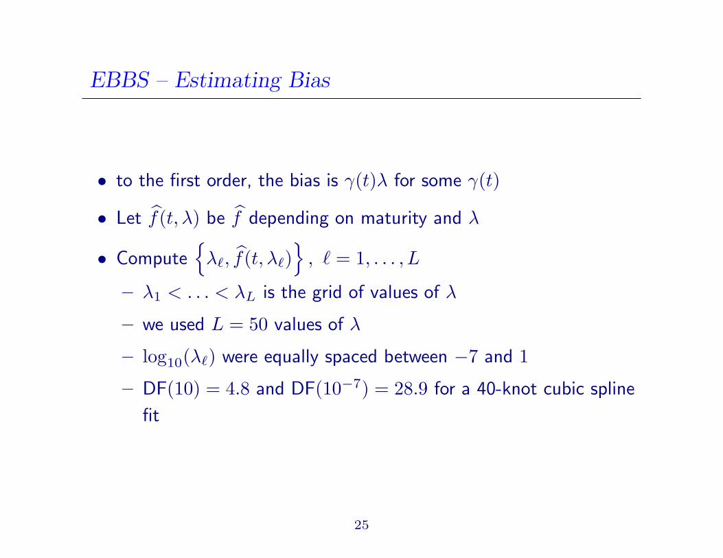
• to the first order, the bias is γ(t)λ for some γ(t)

• Let f(t, λ) be f depending on maturity and λ

• Computeλ`, f(t, λ`)

, ` = 1, . . . , L

– λ1 < . . . < λL is the grid of values of λ

– we used L = 50 values of λ

– log10(λ`) were equally spaced between −7 and 1

– DF(10) = 4.8 and DF(10−7) = 28.9 for a 40-knot cubic spline

fit

25

EBBS – Estimating Bias

• For any fixed t, fit a straight line to the data

(λi, f(t, λi) : i = 1, . . . , L• slope of the line is γ(t)

• estimate of squared bias at t and λ` is (γ(t) λ`)2

26

EBBS versus GCV

0 5 10 15 20 25 30

0.045

0.05

0.055

0.06

0.065

0.07fo

rwar

d ra

te

time to maturity

EBBSGCV θ=3GCV θ=1Empirical

27

EBBS Fit: Residual Analysis

0 10 20 30−6

−4

−2

0

2

4

6x 10

−3

maturity

resi

dual

− lo

g tr

ansf

orm

0 5 10 15 20−0.5

0

0.5

1

Lag

Sam

ple

Aut

ocor

rela

tion

Sample Autocorrelation Function (ACF)

−4 −2 0 2 4 6

x 10−3

0.0030.01 0.02 0.05 0.10

0.25

0.50

0.75

0.90 0.95 0.98 0.99

0.997

Data

Pro

babi

lity

Normal Probability Plot

2.5 3 3.5 4 4.5 50

1

2

3

4

5

6x 10

−3

log(fitted value)

abso

lute

res

idua

l

Residuals from fit using h(·) = log(·)

28

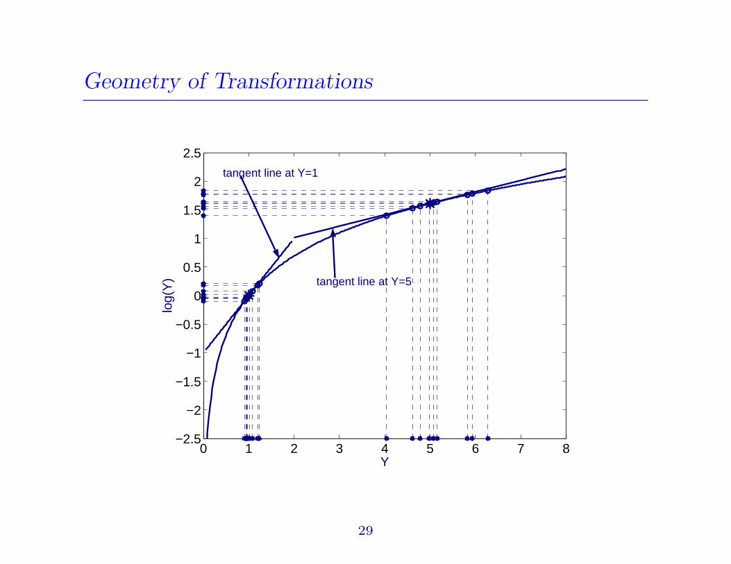
Geometry of Transformations

0 1 2 3 4 5 6 7 8−2.5

−2

−1.5

−1

−0.5

0

0.5

1

1.5

2

2.5

Y

log(

Y) tangent line at Y=5

tangent line at Y=1

29

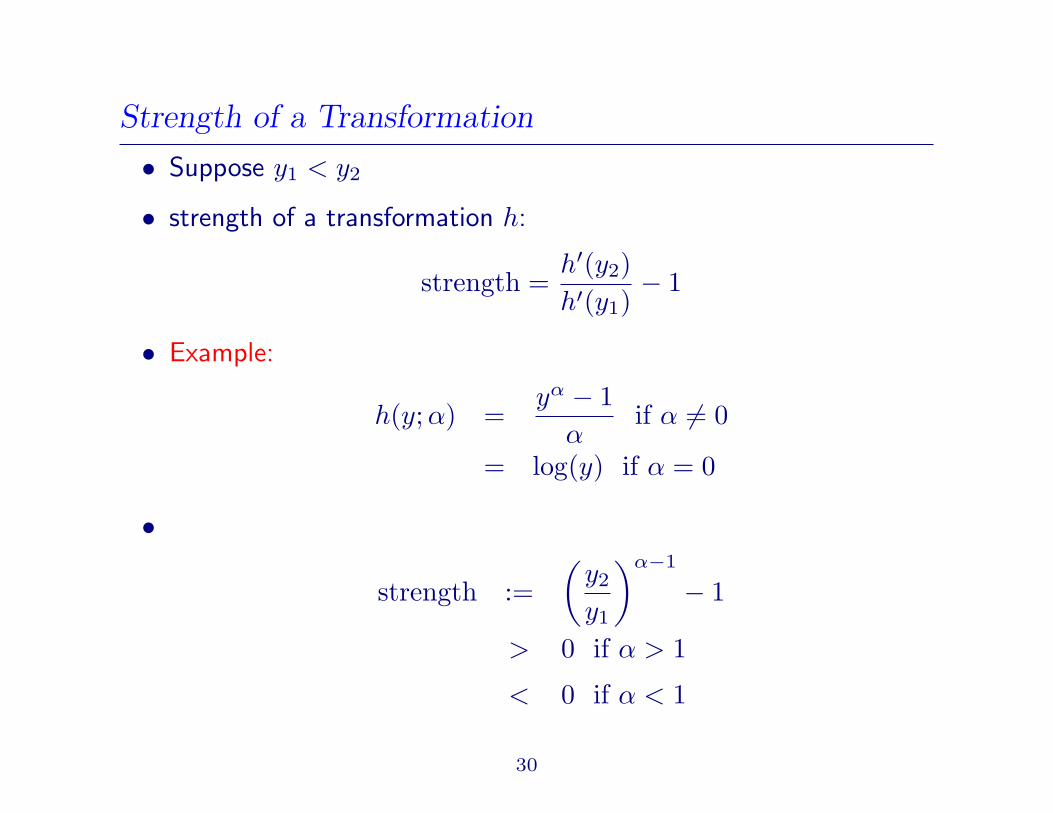
Strength of a Transformation

• Suppose y1 < y2

• strength of a transformation h:

strength =h′(y2)h′(y1)

− 1

• Example:

h(y;α) =yα − 1

αif α 6= 0

= log(y) if α = 0

•

strength :=(

y2

y1

)α−1

− 1

> 0 if α > 1

< 0 if α < 1

30

Strength of a Transformation

−1 −0.5 0 0.5 1 1.5 2

−0.6

−0.4

−0.2

0

0.2

0.4

0.6

0.8

1

alpha

stre

ngth

y2/y

1 = 2

31

Transformation and Weighting

• log is the linearizing transformation

– convenient

– induces some heteroscedasticity, but not enough to cause a

problem

• logP (t)/t = − yield

– cause severe heteroscedasticity – avoid

Transformation and weighting should be done primarily to inducethe assumed noise distribution, which is:

• normal

• constant variance

32

Transformation and Weighting

10 20 30 40 50 60 70 80 90 1000

0.02

0.04

0.06

0.08

0.1

0.12

fitted value

abso

lute

res

idua

lno transform

33

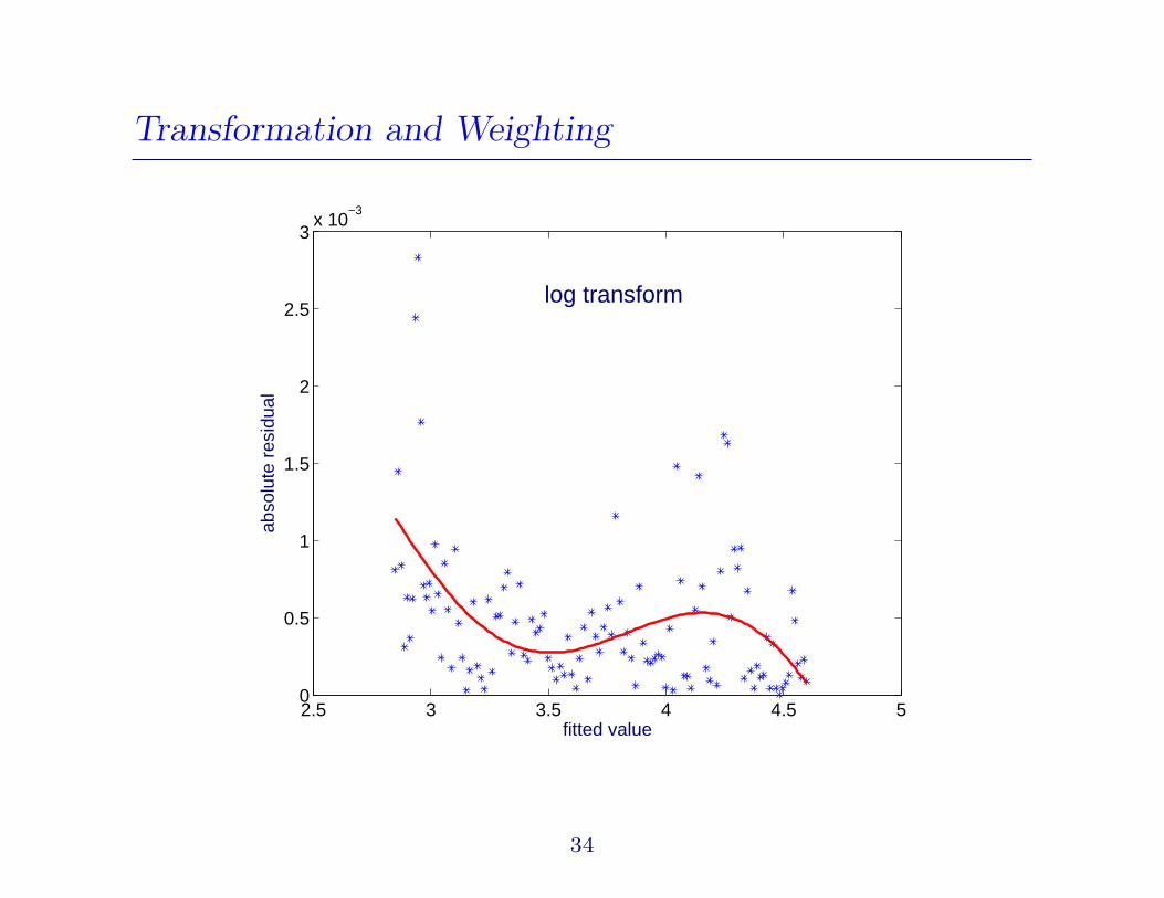
Transformation and Weighting

2.5 3 3.5 4 4.5 50

0.5

1

1.5

2

2.5

3x 10

−3

fitted value

abso

lute

res

idua

l

log transform

34

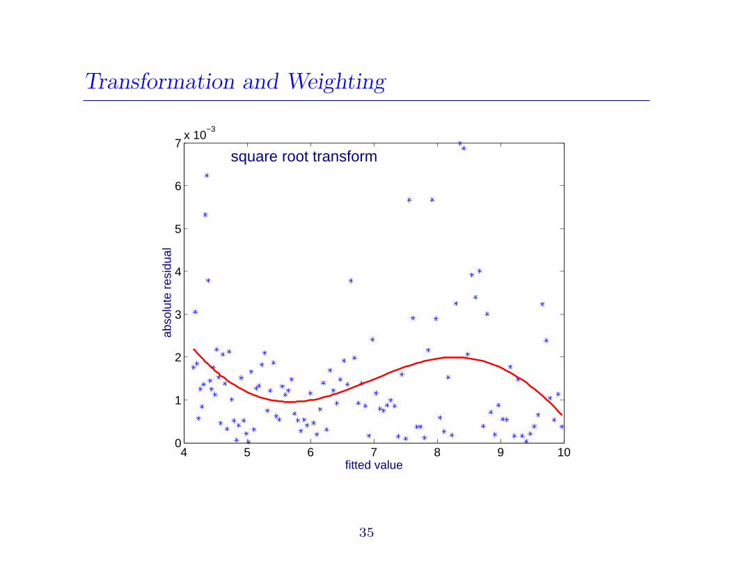
Transformation and Weighting

4 5 6 7 8 9 100

1

2

3

4

5

6

7x 10

−3

fitted value

abso

lute

res

idua

lsquare root transform

35

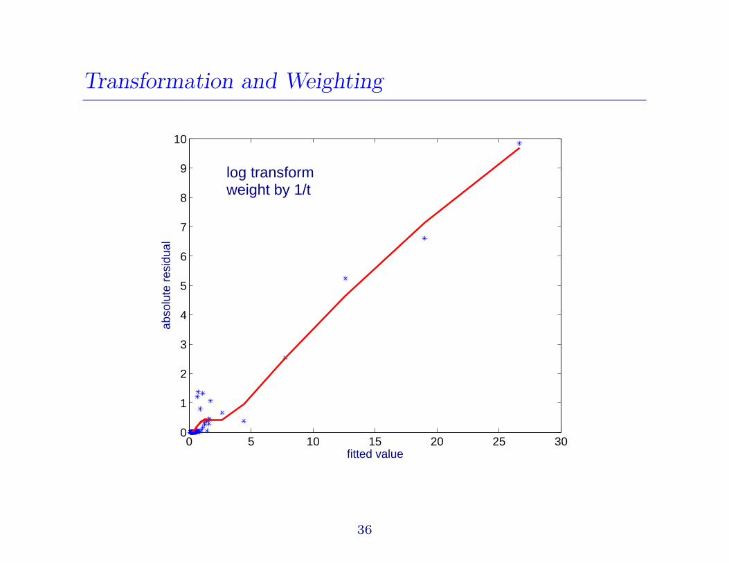
Transformation and Weighting

0 5 10 15 20 25 300

1

2

3

4

5

6

7

8

9

10

fitted value

abso

lute

res

idua

llog transform weight by 1/t

36

Modelling the Correlation

• open problem

• probably not stationary

• simulations show that stationary AR and MA processes do not

have the same problem with GCV as seen with actual price data

37

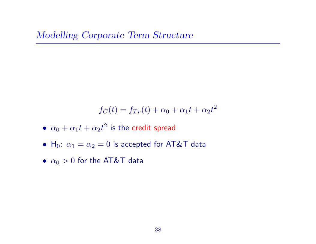
Modelling Corporate Term Structure

fC(t) = fTr(t) + α0 + α1t + α2t2

• α0 + α1t + α2t2 is the credit spread

• H0: α1 = α2 = 0 is accepted for AT&T data

• α0 > 0 for the AT&T data

38

Modelling Corporate Term Structure

0

5

10

15

20

0

5

10

15

20

0.02

0.03

0.04

0.05

0.06

0.07

0.08

0.09

0.1

Years to Maturity

AT&T

Apr 94 − Dec 95

forw

ard

rate

s

39

Modelling Corporate Term Structure

Question: Should one smooth over both date and time to maturity?

40

Asymptotics

The PLS estimator is the solution to

n∑

i=1

ψi(δ, λ,G) = 0

for an appropriate ψi(·, ·, ·)

41

Asymptotics: λ → 0

Theorem 1

• let δn,λn be a sequence of penalized least squares estimators

• assume typical “regularity” assumptions

• suppose λn is o(1)

• then δn is a (strongly) consistent for δ0

• if λn is o(n−1/2), then

√n

(δn,λn − δ0

)D→ N

0, σ2Ω−1(δ0)

,

where

Ω(δ0) := limn

Σn, Σn = σ−2n−1n∑

i=1

Eψi(δ, λ,G)ψi(δ, λ,G)T

42

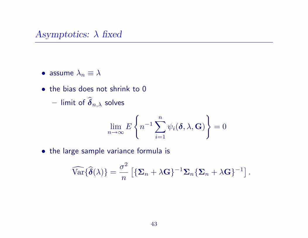
Asymptotics: λ fixed

• assume λn ≡ λ

• the bias does not shrink to 0

– limit of δn,λ solves

limn→∞

E

n−1

n∑

i=1

ψi(δ, λ,G)

= 0

• the large sample variance formula is

Varδ(λ) =σ2

n

[Σn + λG−1ΣnΣn + λG−1].

43

Summary

• splines are convenient for estimating term structure

• penalization is better, or at least easier, than knot selection

• EBBS provides a reasonable amount of smoothing

• GCV undersmooths because

– noise is correlated

– target function is a derivative

• corporate term structure can be estimated by “borrowing

strength” from treasury bonds

• a constant credit spread fits the data reasonably well

• asymptotics are available for inference

44

References

Jarrow, R., Ruppert, D., and Yu, Y. (2004) Estimating the interest

rate term structure of corporate debt with a semiparametric

penalized spline model, JASA, to appear.

Available at:

http://www.orie.cornell.edu/~davidr

• see “Recent Papers”

• also see “Recent Talks” for these slides

45

References

Ruppert, D. (2004) Statistics and Finance: An Introduction,

Springer, New York – splines, term structure, transformations

Ruppert, D., Wand, M.P., and Carroll, R.J. (2003) Semiparametric

Regression, Cambridge University Press, New York – splines

Carroll, R.J. and Ruppert, D. (1988), Transformation and Weighting

in Regression, Chapman & Hall, New York. – transform-both-sides

46