Estimating spatial panel models using unbalanced data€¦ · Estimating spatial panel models using...
25
Estimating spatial panel models using unbalanced data Gordon Hughes University of Edinburgh Andrea Piano Mortari & Federico Belotti CEIS, Universita Roma Tor Vergata 12 th September 2013
Transcript of Estimating spatial panel models using unbalanced data€¦ · Estimating spatial panel models using...

Estimating spatial panel models using unbalanced data
Gordon HughesUniversity of Edinburgh
Andrea Piano Mortari & Federico BelottiCEIS, Universita Roma Tor Vergata
12th September 2013
12 September 2013 2
Outline
Reasons for using spatial panel models?Spatial interactions – e.g. tax & environmental policiesSpatial spillovers – migration or relocation of industrial activityControlling for spatially-correlated omitted variables
Econometric models, data and softwareSpatial lags & errors – parallels with time series modelsStata, R & Matlab – community routines
Unbalanced panelsChanges in population of countries, states, etcSpatial interactions with missing data
US electricity demand by statePrice effects and regulation
12 September 2013 3
Spatial analysis in Stata
Variety of special purpose routines written by users and available through SSC
Manipulation of spatial dataCross-section spatial regressions
StataCorp-related routines – also through SSCshp2dta converts ESRI shapefiles to dta files – similar to programs converting to csv or xls filesspmat, spreg, spivreg, etc for construction & manipulation of spatial weights and for cross-section spatial regressions

12 September 2013 4
Nature of spatial panel data
Large N and/or large T?Missing data and spatial weights
Contiguity vs inverse distanceTo (row) standardise or not?
Examples: Energy demand – gasoline, electricity, etc State tax and fiscal policiesCross-country models of economic development Spatial hedonic models & hedonic valuation

12 September 2013 5
Econometric specification
Fixed or random effects – can we talk about random effects with complete sample of states or countries?Lagged dependent variable or within panel serial correlationWhy are data missing – missing at random assumption

12 September 2013 6
Key models
Spatial auto-regression model (SAR)
Spatial Durbin model (SDM)
Spatial autocorrelation model (SAC)
it t it i ity Wy X
it t it t i ity Wy X WX
t t t t t t ty Wy X with Mv

12 September 2013 7
Key models 2
Spatial error model (SEM)
Generalised spatial random errors (GSPRE)
it it i it it t ity X with Wv
1 2t t t t t ty X with W and M

12 September 2013 8
Procedure xsmle - syntax
xsmle varlist [if] [in] [weight], WMATrix(string) [MODel(string) FE RE EMATrix(string) DMATrix DURBin(varlist) ROBust DKRAAY(#) DLAG ERRor(#) NOConstant]"varlist" = depvar indvars [required]."wmat(WN)", “emat(WE)”, “dmat(WD)” refer to an N x N matrices of spatial weights for spatial lags, spatial errors and Durbin variables [at least one of wmat() or emat() is required].“model(string)” specifies the type of model to be estimated. The default is “sar” and alternatives are “sdm”, “sem”, “sac” and “gspre”. “fe | re" specifies that a fixed or random effects model should be used – the default varies according to the model specified.

12 September 2013 9
Procedure xsmle – syntax 2
“durbin(varlist)” specifies a set of spatially-weighted regressors.“vce()” specified type of variance-covariance estimator – options include likelihood-based and sandwich estimators:
hessians from optimization – vce(oim), vce(opg); panel & cluster robust standard error – vce(robust) vce(cluster clusvar);Driscoll-Kraay variant of Newey-West robust standard errors with default or specific lag – vce(dkraay #)
"dlag" includes the lagged dependent variable in the model. This is only available for model(sar) and model(sdm).“err(#)” specifies the error structure for the GSPRE model. The default is the most general version ( 1 2 0). "noconstant" specifies that the model should be estimated without adding a constant term.

12 September 2013 10
Features of xsmle
Fast for N ~ 500, copes with N ~ 2000Memory & multiple core processing beneficial
Full range of Stata options for ML estimation and post-estimationQuite general syntax & options
Multiple sets of spatial weights for different componentsSelection of Durbin variablesBoth individual and time fixed effects permittedAnalytical & important weights permitted
Generates estimates of direct & indirect impacts plus associated standard errors (by Monte Carlo sampling)
12 September 2013 11
Illustration – US electricity demand
State data – continental US, 1990-2011Electricity demand by sectorRegressors - prices, weather (heating & cooling days)
Focus on price elasticities and weather impactsLikely to be spatial interactions due to
Common factors in unobserved variablesCompetition between states for industry and/or movement of households
12 September 2013 12
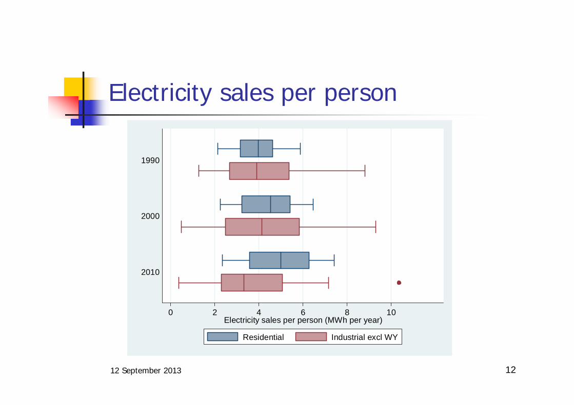
Electricity sales per person
0 2 4 6 8 10Electricity sales per person (MWh per year)
2010
2000
1990
Residential Industrial excl WY
12 September 2013 13
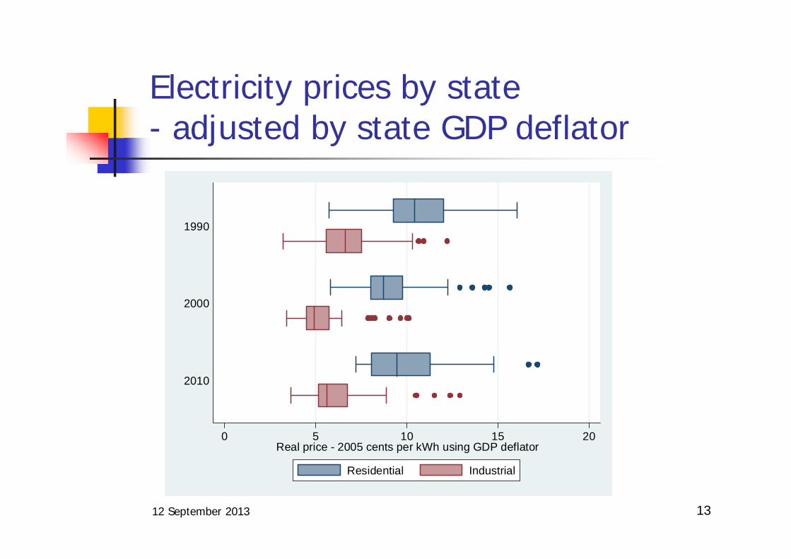
Electricity prices by state- adjusted by state GDP deflator
0 5 10 15 20Real price - 2005 cents per kWh using GDP deflator
2010
2000
1990
Residential Industrial

12 September 2013 14
Residential demand - FE models

12 September 2013 15
Unbalanced panels - options
Listwise deletionCan mean loss of all or most of sample
ML estimation of joint modelPfaffermayr for GSPRE model
Treating panel as pooled cross-sectionImputation
Single imputation can be useful for spatial lags but see Cameron & TrivediMultiple imputation using Monte Carlo chain approach
12 September 2013 16
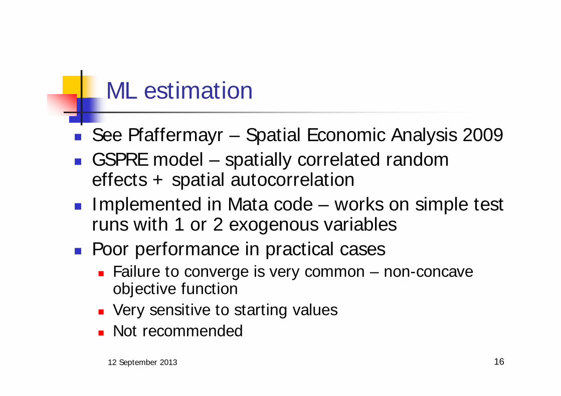
ML estimation
See Pfaffermayr – Spatial Economic Analysis 2009GSPRE model – spatially correlated random effects + spatial autocorrelationImplemented in Mata code – works on simple test runs with 1 or 2 exogenous variablesPoor performance in practical cases
Failure to converge is very common – non-concave objective functionVery sensitive to starting valuesNot recommended

12 September 2013 17
Pooled cross-section estimation 1
See Baltagi et al – Journal of Econometrics 2007 & Egger et al – Economics Letters 2005Pool cross sections with different sets of panel units (countries) for each period
Create spatial weights Wt for each t by row/col deletion and (perhaps) standardisationFull matrix of spatial weights is block diagonal with W1.. WT as the diagonal elements
Estimate using cross-section spatial procedure such as –spreg- including panel unit dummies for fixed effects

12 September 2013 18
Pooled cross-section estimation 2
Implemented in Mata with –spmat- and –spreg-Good execution speed and seems robust
Conceptual issuesHow to interpret time-varying spatial interactions?
Reasonable when the population is changing – e.g. units splitting up or mergingArbitrary exclusion when driven by missing dataShould the Wt be row-standardised?
Missing data leads to islands with contiguity weightsTests: coefficients are severely biased with potentially serious impact on hypothesis tests

12 September 2013 19
Multiple imputation
-xsmle- has been set up to permit use with –mi-Care is needed in specifying the method of imputation that is used – tests use regression imputation controlling for state effectsSignificant cost of setting up & testing the imputation frameworkAfter this the computational cost is reasonable so advice is to use M > % of missing data
Less expensive than bootstrap standard errors – at least with a proper number of repetitions
12 September 2013 20
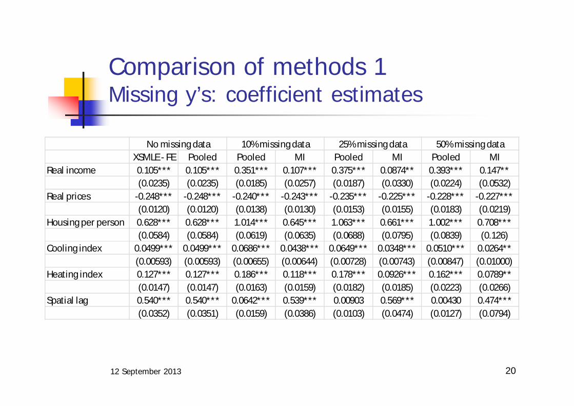
Comparison of methods 1Missing y’s: coefficient estimates
No missing data 10% missing data 25% missing data 50% missing dataXSMLE - FE Pooled Pooled MI Pooled MI Pooled MI
Real income 0.105*** 0.105*** 0.351*** 0.107*** 0.375*** 0.0874** 0.393*** 0.147**(0.0235) (0.0235) (0.0185) (0.0257) (0.0187) (0.0330) (0.0224) (0.0532)
Real prices -0.248*** -0.248*** -0.240*** -0.243*** -0.235*** -0.225*** -0.228*** -0.227***(0.0120) (0.0120) (0.0138) (0.0130) (0.0153) (0.0155) (0.0183) (0.0219)
Housing per person 0.628*** 0.628*** 1.014*** 0.645*** 1.063*** 0.661*** 1.002*** 0.708***(0.0584) (0.0584) (0.0619) (0.0635) (0.0688) (0.0795) (0.0839) (0.126)
Cooling index 0.0499*** 0.0499*** 0.0686*** 0.0438*** 0.0649*** 0.0348*** 0.0510*** 0.0264**(0.00593) (0.00593) (0.00655) (0.00644) (0.00728) (0.00743) (0.00847) (0.01000)
Heating index 0.127*** 0.127*** 0.186*** 0.118*** 0.178*** 0.0926*** 0.162*** 0.0789**(0.0147) (0.0147) (0.0163) (0.0159) (0.0182) (0.0185) (0.0223) (0.0266)
Spatial lag 0.540*** 0.540*** 0.0642*** 0.539*** 0.00903 0.569*** 0.00430 0.474***(0.0352) (0.0351) (0.0159) (0.0386) (0.0103) (0.0474) (0.0127) (0.0794)
12 September 2013 21
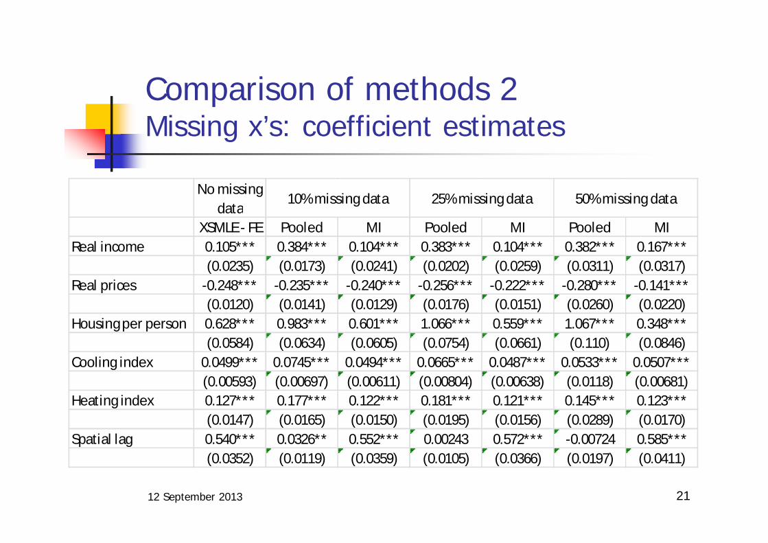
Comparison of methods 2Missing x’s: coefficient estimates
No missing data
10% missing data 25% missing data 50% missing data
XSMLE - FE Pooled MI Pooled MI Pooled MIReal income 0.105*** 0.384*** 0.104*** 0.383*** 0.104*** 0.382*** 0.167***
(0.0235) (0.0173) (0.0241) (0.0202) (0.0259) (0.0311) (0.0317)Real prices -0.248*** -0.235*** -0.240*** -0.256*** -0.222*** -0.280*** -0.141***
(0.0120) (0.0141) (0.0129) (0.0176) (0.0151) (0.0260) (0.0220)Housing per person 0.628*** 0.983*** 0.601*** 1.066*** 0.559*** 1.067*** 0.348***
(0.0584) (0.0634) (0.0605) (0.0754) (0.0661) (0.110) (0.0846)Cooling index 0.0499*** 0.0745*** 0.0494*** 0.0665*** 0.0487*** 0.0533*** 0.0507***
(0.00593) (0.00697) (0.00611) (0.00804) (0.00638) (0.0118) (0.00681)Heating index 0.127*** 0.177*** 0.122*** 0.181*** 0.121*** 0.145*** 0.123***
(0.0147) (0.0165) (0.0150) (0.0195) (0.0156) (0.0289) (0.0170)Spatial lag 0.540*** 0.0326** 0.552*** 0.00243 0.572*** -0.00724 0.585***
(0.0352) (0.0119) (0.0359) (0.0105) (0.0366) (0.0197) (0.0411)

12 September 2013 22
Comparison of methods 3Missing y’s - absolute bias as % of full se
No missing data
10% missing data 25% missing data 50% missing data
Pooled Pooled MI Pooled MI Pooled MIReal income 0% 1047% 9% 1149% 77% 1226% 179%Real prices 0% 67% 42% 108% 192% 167% 175%Housing per person 0% 661% 29% 745% 57% 640% 137%Cooling index 0% 315% 103% 253% 255% 19% 396%Heating index 0% 401% 61% 347% 238% 238% 333%Spatial lag 0% 1352% 3% 1509% 82% 1523% 188%
12 September 2013 23
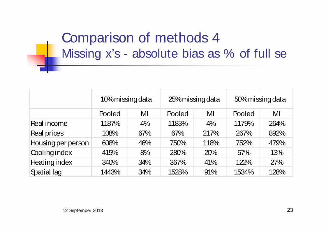
Comparison of methods 4Missing x’s - absolute bias as % of full se
10% missing data 25% missing data 50% missing data
Pooled MI Pooled MI Pooled MIReal income 1187% 4% 1183% 4% 1179% 264%Real prices 108% 67% 67% 217% 267% 892%Housing per person 608% 46% 750% 118% 752% 479%Cooling index 415% 8% 280% 20% 57% 13%Heating index 340% 34% 367% 41% 122% 27%Spatial lag 1443% 34% 1528% 91% 1534% 128%

Comparison of methods: lessons
Be careful about use of either ML estimation or pooled cross section unless
The model specification is simple and convergence is reliable for MLIn cases of a changing population of panel units for which pooled cross section may be appropriate
When using multiple imputationTest several different methods of imputationUse as many imputations as you can afford to run
12 September 2013 24

12 September 2013 25
Why spatial analysis matters:results for US electricity
Clear evidence of spatial spillovers in electricity demand –especially for residential use
Coefficients on spatial lag in range 0.3-0.45Allowing for spatial effects significantly reduces the coefficients on real income & housingHigher electricity prices in one state associated with higher consumption in neighbouring states
Policy: State renewable portfolio standards (RPS)Potential price increases to 2020 up to 40%How much effect on consumption and CO2 emissions?