
Focusing High-Resolution Highly-Squinted Airborne SAR Data ...

General rights Copyright and moral rights for the publications made accessible in the public portal are retained by the authors and/or other copyright owners and it is a condition of accessing publications that users recognise and abide by the legal requirements associated with these rights.
Users may download and print one copy of any publication from the public portal for the purpose of private study or research.
You may not further distribute the material or use it for any profit-making activity or commercial gain
You may freely distribute the URL identifying the publication in the public portal If you believe that this document breaches copyright please contact us providing details, and we will remove access to the work immediately and investigate your claim.
Downloaded from orbit.dtu.dk on: Jul 03, 2019
Estimating Sensor Motion in Airborne SAR
Kusk, Anders
Publication date:2006
Document VersionPublisher's PDF, also known as Version of record
Link back to DTU Orbit
Citation (APA):Kusk, A. (2006). Estimating Sensor Motion in Airborne SAR. Kgs. Lyngby: Technical University of Denmark(DTU).

Estimating Sensor Motion in Airborne SAR
Ph.D.-Thesis
Anders Kusk
Ørsted•DTU
Supervisors
Jørgen Dall
Erik Lintz Christensen
10 May 2006


Abstract
In airborne synthetic aperture radar (SAR), accurate knowledge of the SAR sensormotion is necessary to achieve an acceptable image quality with respect to resolution,image artifacts and geometrical distortions. For repeat-track interferometry, whereSAR images acquired from different passes are combined, the absolute accuracy re-quirements are even more stringent, as small residual errors will be misinterpretedas scene displacements or topography.
This thesis deals with two aspects of motion estimation in airborne SAR. The firstpart is an examination of the impact of propeller aircraft vibrations on SAR focus-ing. Uncompensated high-frequency motion leads to sidelobes (false echoes) in SARimages. Motion measurements from two propeller aircraft are presented and evalu-ated with respect to their high-frequency content, and the impact of the measuredmotion on the image quality is predicted. The motion measurements are comparedto similar measurements on a jet aircraft. It is shown that narrowband vibrationsat harmonics of the propeller frequency appear in the motion data for the propelleraircraft, and that vibration levels for the jet are significantly lower. It is predictedthat the levels of the measured physical vibrations do not lead to unacceptable side-lobes if left uncompensated, but aliasing of the vibrations in the INU can inducespurious low-frequency vibrations at the aliased frequencies in the navigation data.This leads to incorrect motion compensation, and since the aliased vibrations canhave higher levels than the actual vibrations due to the integration processes in theINU, unacceptable sidelobes may result.
The second part of the thesis deals with correction of differential motion errors inairborne repeat track SAR interferometry. The work extends an existing differentialmotion estimation algorithm that integrates the azimuth misregistration to obtainan estimate of the differential motion error between the images. In this thesis, thealgorithm is analysed, and potential error sources are identified and examined. Oneerror source is azimuth misregistrations from performing motion compensation withunknown topography. A simple method for reducing topography-induced errors usingan external DEM is proposed, and it seems to slightly improve the motion estimateon the L-band EMISAR data for which it was tested.
Another error source in the residual motion algorithm is along-track residual motionerrors, which lead to azimuth misregistrations that can be interpreted wrongly asvertical velocity errors. A method is proposed for estimating and correcting theseerrrors using an external DEM or - as is possible in some cases - the residual rangemisregistration. The proposed method is tested on a 100 km C-band scene, for whichthe observed residual cross-track error was still on the order of 15 cm after the initialcorrection. This variation was reduced to below 2 cm over a 60 km long strip inazimuth.


Resumé
I flybåren syntetisk apertur radar (SAR) er nøjagtigt kendskab til SAR-sensorensbevægelser nødvendig for at opnå en acceptabel billedkvalitet med hensyn til opløs-ning, falske ekkoer og geometrisk forvrængning. Hvis der skal udføres repeat-trackinterferometri, hvor flere SAR-billeder optaget fra separate spor kombineres, bliverkravene til absolut nøjagtighed endnu strengere, da små restfejl kan blive misfortolketsom forskydninger i scenen, eller som hidrørende fra topografien.
Denne afhandling beskæftiger sig med to aspekter af bevægelsesestimation i flybå-ren SAR. I første del undersøges indflydelsen af vibrationer i propelfly på SAR-fokuseringen. Ukompenserede højfrekvente bevægelser af SAR-sensoren kan føre tilsidesløjfer (falske ekkoer) i fokuserede SAR-billeder. Bevægelsesmålinger fra to pro-pelfly præsenteres og analyseres med hensyn til deres højfrekvensindhold, og denforventede indflydelse af de målte bevægelser på SAR-fokuseringen beregnes. Bevæ-gelsesmålingerne sammenlignes med tilsvarende målinger for et jetfly. Det eftervisesat harmoniske af propelfrekvensen dukker op i de målte bevægelser for propelflyene,og at vibrationsniveauerne for jetflyet er betydeligt lavere end disse. Med de måltevibrationsniveauer forventes det ikke at de fysiske vibrationer fører til uacceptablesidesløjfer, hvis de ikke kompenseres. Dog kan aliasering af højfrekvente vibrationeri INU’en introducere falske lav-frekvente vibrationer ved den aliaserede frekvens ibevægelsesdata. Dette fører til fejl i bevægelseskompensationen, og på grund af denintegration, der foretages i INU’en, kan de aliaserede vibrationer have højere niveauerend de fysiske vibrationer, og dette kan føre til uacceptable sidesløjfeniveauer.
Anden del af afhandligen beskæftiger sig med korrektion af restbevægelsesfejl i flybå-ren repeat-track SAR interferometri. Det udførte arbejde tager udgangspunkt i eneksisterende algoritme til estimation af restbevægelsesfejl, der fungerer ved at in-tegrere azimuth-misregistreringen mellem to SAR-billeder. I denne afhandling ana-lyseres algoritmen, og potentielle fejlkilder identificeres og undersøges. Én fejlkildeer azimuth-misregistreringer forårsaget af topografi-uafhængig bevægelseskompen-sation. Der foreslås en simpel metode til at reducere sådanne fejl vha. en externhøjdemodel, og metoden ser ud til at medføre en lille forbedring af estimatet afrestbevægelsesfejlen for de L-bånds EMISAR data metoden blev afprøvet på.
En anden fejlkilde er restbevægelsesfejl i flyveretningen. Disse fører til azimuth-misregistrering, som fejlagtigt tolkes som restfejl i tværretningen. Der foreslås enmetode til at estimere og korrigere sådanne fejl ved hjælp af en extern højdemodeleller - som det i nogle tilfælde er muligt - misregistreringen i range-retningen. Denforeslåede metode testes på en 100 km lang C-bånds-scene, for hvilken restbevægelses-fejlen stadig var af størrelsesordenen 15 cm efter korrektionen af restbevægelsesfejlenmed den originale algoritme. Denne fejl reduceres med den ny metode til under 2 cmover en 60 km lang stribe i azimuth-retningen.


Contents
1 Introduction 1
2 Motion Errors in SAR Focusing 3
2.1 Basic SAR theory . . . . . . . . . . . . . . . . . . . . . . . . . . . . . 3
2.1.1 Definitions and assumption . . . . . . . . . . . . . . . . . . . 3
2.1.2 Focusing with nominal sensor motion . . . . . . . . . . . . . . 4
2.2 Motion compensation . . . . . . . . . . . . . . . . . . . . . . . . . . . 5
2.2.1 Sensor track with non-ideal motion . . . . . . . . . . . . . . . 5
2.2.2 Motion compensation procedure . . . . . . . . . . . . . . . . 6
2.2.3 Residual motion errors . . . . . . . . . . . . . . . . . . . . . . 7
2.3 Impact of motion errors on focusing . . . . . . . . . . . . . . . . . . 9
2.3.1 Constant and linear motion errors . . . . . . . . . . . . . . . 9
2.3.2 Higher order motion errors . . . . . . . . . . . . . . . . . . . 10
2.4 Estimation of sensor motion . . . . . . . . . . . . . . . . . . . . . . . 13
3 Aircraft Vibrations and SAR Focusing 15
3.1 Motion sensor description . . . . . . . . . . . . . . . . . . . . . . . . 17
3.1.1 EGI coordinate systems . . . . . . . . . . . . . . . . . . . . . 17
3.1.2 EGI navigation processing . . . . . . . . . . . . . . . . . . . . 18
3.1.3 EGI high frequency characteristics . . . . . . . . . . . . . . . 21
3.1.4 Selection of motion variables for vibration measurements . . . 21
3.2 Measurements . . . . . . . . . . . . . . . . . . . . . . . . . . . . . . . 23
3.2.1 C-130 measurement setup . . . . . . . . . . . . . . . . . . . . 23
3.2.2 Piper PA31 measurement setup . . . . . . . . . . . . . . . . . 23
3.2.3 GIII measurement setup . . . . . . . . . . . . . . . . . . . . . 25
3.2.4 Summary of flight conditions . . . . . . . . . . . . . . . . . . 25
3.3 Vibration analysis . . . . . . . . . . . . . . . . . . . . . . . . . . . . 25
3.3.1 Model for small aircraft vibrations . . . . . . . . . . . . . . . 25
3.3.2 Estimating vibration measurement errors . . . . . . . . . . . 27

viii CONTENTS
3.3.3 Assumed SAR system description . . . . . . . . . . . . . . . . 28
3.3.4 Motion data processing . . . . . . . . . . . . . . . . . . . . . 28
3.3.5 PSLR estimation . . . . . . . . . . . . . . . . . . . . . . . . . 29
3.4 C-130 measurements . . . . . . . . . . . . . . . . . . . . . . . . . . . 31
3.4.1 Motion spectra . . . . . . . . . . . . . . . . . . . . . . . . . . 31
3.4.2 C-130 PSLR evaluation . . . . . . . . . . . . . . . . . . . . . 34
3.4.3 Aliasing of motion data . . . . . . . . . . . . . . . . . . . . . 35
3.5 Piper PA31 measurements . . . . . . . . . . . . . . . . . . . . . . . . 37
3.5.1 Motion spectra . . . . . . . . . . . . . . . . . . . . . . . . . . 37
3.5.2 PA31 PSLR Evaluation . . . . . . . . . . . . . . . . . . . . . 41
3.6 Gulfstream GIII measurements . . . . . . . . . . . . . . . . . . . . . 43
3.6.1 Motion spectra . . . . . . . . . . . . . . . . . . . . . . . . . . 43
3.7 Discussion . . . . . . . . . . . . . . . . . . . . . . . . . . . . . . . . . 43
4 Motion Errors in Repeat Track Interferometry 47
4.1 Basic principles of interferometry . . . . . . . . . . . . . . . . . . . . 48
4.1.1 Geometry . . . . . . . . . . . . . . . . . . . . . . . . . . . . . 48
4.1.2 Interferometric phase errors . . . . . . . . . . . . . . . . . . . 50
4.1.3 The complex coherence . . . . . . . . . . . . . . . . . . . . . 51
4.2 Motion errors in interferometry . . . . . . . . . . . . . . . . . . . . . 51
4.2.1 Impact of motion errors . . . . . . . . . . . . . . . . . . . . . 52
4.2.2 Impact of topography . . . . . . . . . . . . . . . . . . . . . . 55
4.2.3 Summary of motion error model . . . . . . . . . . . . . . . . 56
4.3 Estimating misregistration . . . . . . . . . . . . . . . . . . . . . . . . 57
4.3.1 Spectral Diversity Coregistration (SDC) . . . . . . . . . . . . 57
4.4 Estimating differential motion errors . . . . . . . . . . . . . . . . . . 59
4.4.1 Parametric motion error estimation . . . . . . . . . . . . . . . 59
4.4.2 Non-parametric motion error estimation . . . . . . . . . . . . 60
4.4.3 Estimating constant differential motion errors . . . . . . . . . 62
4.5 Correcting differential motion errors . . . . . . . . . . . . . . . . . . 63
5 Improved Non-parametric Motion Error Estimation 67
5.1 Along-track errors . . . . . . . . . . . . . . . . . . . . . . . . . . . . 67
5.1.1 Estimating along-track errors using External DEM . . . . . . 69
5.1.2 Summary of algorithm . . . . . . . . . . . . . . . . . . . . . . 72
5.2 Impact of topography . . . . . . . . . . . . . . . . . . . . . . . . . . 72
5.2.1 Accounting for spherical Earth geometry . . . . . . . . . . . . 72

CONTENTS ix
5.2.2 External DEM projection to slant range geometry . . . . . . 73
5.2.3 Generation of synthetic interferogram . . . . . . . . . . . . . 74
5.2.4 Modeling azimuth misregistration from topography . . . . . . 74
5.3 Implementation . . . . . . . . . . . . . . . . . . . . . . . . . . . . . . 75
5.3.1 Implementation of SDC and RME algorithms . . . . . . . . . 77
5.3.2 Implementation of improved RME . . . . . . . . . . . . . . . 78
6 Experimental Evaluation 79
6.1 Data processing . . . . . . . . . . . . . . . . . . . . . . . . . . . . . . 79
6.2 Evaluation with L-band data . . . . . . . . . . . . . . . . . . . . . . 80
6.2.1 Initial processing . . . . . . . . . . . . . . . . . . . . . . . . . 80
6.2.2 SDC processing . . . . . . . . . . . . . . . . . . . . . . . . . . 84
6.2.3 RME estimation and correction . . . . . . . . . . . . . . . . . 85
6.2.4 Along-track motion estimation . . . . . . . . . . . . . . . . . 88
6.3 Evaluation with C-band data . . . . . . . . . . . . . . . . . . . . . . 95
6.3.1 Inital processing . . . . . . . . . . . . . . . . . . . . . . . . . 95
6.3.2 SDC processing . . . . . . . . . . . . . . . . . . . . . . . . . . 97
6.3.3 RME estimation . . . . . . . . . . . . . . . . . . . . . . . . . 100
6.3.4 Along-track error estimation . . . . . . . . . . . . . . . . . . . 101
6.4 Discussion . . . . . . . . . . . . . . . . . . . . . . . . . . . . . . . . . 106
7 Conclusions 109
7.1 Vibration analysis . . . . . . . . . . . . . . . . . . . . . . . . . . . . 109
7.2 Residual motion errors in RTI . . . . . . . . . . . . . . . . . . . . . . 109
7.3 Acknowledgements . . . . . . . . . . . . . . . . . . . . . . . . . . . . 111


Chapter 1
Introduction
Synthetic Aperture Radar (SAR) is a well-established technology for remote sensing,and has applications in geophysics, topographic mapping, disaster management andmany other areas. Numerous space- and airborne systems have been built and flown.Spaceborne systems have the advantage of wide coverage, whereas airborne systemshave a higher degree of freedom in the choice of imaging geometry and revisit times.Also, due to the shorter range to the imaged area, airborne SAR systems achievehigher signal-to-noise ratios than spaceborne systems.
The subject of this thesis is estimation of sensor motion in airborne SAR, a subjectwhich has seen much attention. Accurate knowledge of the SAR sensor motion iscritical to achieve a good focusing quality. With the introduction in the 1990’s ofintegrated Inertial (INU) and GPS navigation solutions, acceptable image qualitycan now be obtained without autofocusing algorithms. The INU is still necessaryto estimate the high-frequency content of the motion, whereas the GPS corrects forthe slowly varying drift of the INU. However, even with kinematic GPS, absolutepositioning errors of 5-10 cm are still seen.
In this work, two aspects of airborne SAR motion estimation are examined. Thefirst part is an examination of the impact of propeller-induced vibrations on thefocusing quality in high-performance SAR systems mounted on propeller aircraft.This was motivated by the now discontinued SAR++ program [1] at Ørsted•DTU,in which, among other configurations, high-resolution (25 cm) SAR systems at C-and X-band frequencies with strict sidelobe level requirements were studied. It iswell known that uncompensated sinusoidal motion errors can lead to sidelobes in theSAR impulse response, and it is conceivable that such errors could be introducedby propeller motion. To examine this, high-frequency INU motion data from aLockheed-Martin C-130 Hercules were collected as part of this study. These motiondata were compared to motion data from a small propeller aircraft, a Piper PA31Navajo and, for reference, a GIII Gulfstream jet aircraft. Spectral analysis andpoint target simulations have been performed to estimate the impact on the focusingquality of a hypothetical SAR system mounted on one of these aircraft.
The second, and major, part of the thesis deals with estimation of differential mo-tion errors in airborne repeat track SAR interferometry (RTI). SAR Interferometryis a powerful technique that can be used to detect small shifts between two SARimages acquired from different tracks. In single-pass interferometry (often referredto as across-track interferometry, or XTI), the images are acquired simultaneously

2 Introduction
from two antennas mounted on the same aircraft. In this case, the observed phaseshifts are related to the scene topography, and therefore XTI systems are often usedfor generation of digital elevation models (DEMs). In repeat track interferometry,the SAR images are acquired at different times, and the interferometric phase shiftcontains contributions both from the topography and from temporal changes in theimaged scene. This can be used to detect small displacements, for example due tolandslides or glacial motion. Also, the possibility of a large baseline not limited bythe aircraft dimensions allows a higher sensitivity to topography. However, sincethe motion errors in the two different acquisitions are generally not correlated, thedifference in the motion errors is directly seen in the interferometric phase. Since thedesired interferometric range shifts are often smaller than the 5-10 cm motion esti-mation errors which is state-of-the-art with kinematic GPS, calibration techniquesusing the acquired data must be applied. This may be augmented by using tie-pointsin the image or an external elevation model. Another problem is phase errors causedby atmospheric delays. The interferometric range shift from such errors can be upto several centimeters, so for high-precision applications this cannot be ignored.
In this work, an existing method [2] for differential motion error estimation in air-borne RTI has been examined. The method is based on integration of the observedazimuth misregistration between the images to obtain a non-parametric estimate ofthe differential motion error. This is based on the assumption that the observed az-imuth misregistration is entirely due to uncompensated cross-track velocities. How-ever, azimuth misregistrations are also caused by along-track motion errors, and byperforming motion compensation with unknown topography. The contributions fromthese sources of misregistration on the differential motion estimate have been anal-ysed in this work, and methods have been developed for correcting for them using acoarse external DEM. Finally, the original algorithm has been applied to EMISARdata, and the suggested improvements have also been applied. The influence of theatmosphere on the interferometric phase has not been covered.
The thesis starts with a brief review of SAR motion compensation in Chapter 2.This is followed by the vibration analysis in Chapter 3. In Chapter 4, a brief reviewof motion errors in SAR interferometry is given, followed by a description of thedifferential motion estimation algorithm on which this work is based. The analysisand suggested improvements to the algorithm is presented in Chapter 5, and theexperimental verification using EMISAR data is presented in Chapter 6, togetherwith a discussion of the achieved results. Finally, the conclusion is presented inChapter 7.

Chapter 2
Motion Errors in SAR Focusing
In this chapter, the origin and impact of sensor motion errors in airborne SAR arediscussed. First, basic SAR focusing and motion compensation theory is presented.Then the impact of motion estimation and compensation errors on the focused SARimage is analysed. The topic of SAR motion errors and compensation has beendiscussed widely in the literature, e.g. [3, 4, 5], and the theory in this chapter isbased on the literature.
xy
z
r0
(xT , yT , zT )
(xR, yR, zR)
Figure 2.1: Simplified SAR geometry.
2.1 Basic SAR theory
2.1.1 Definitions and assumption
A simplified broadside looking SAR geometry is shown in Figure 2.1. An (x, y, z)coordinate system is defined such that the reference track, to which the SAR imageis focused, can be described by the nominal position vector pR(x) = (x, 0, zR), wherezR is the (constant) reference track altitude. In these coordinates the target position

4 Motion Errors in SAR Focusing
is pT = (xT , yT , zT ).
For analysing the airborne SAR focusing process, it is sufficient to assume a flat Earthgeometry, since the flat Earth approximation simplifies the analysis and has littleimpact on the focusing quality. A spherical geometry that accounts more accuratelyfor the curvature of the sensor track is in the following chapters adopted whereappropriate.
2.1.2 Focusing with nominal sensor motion
With nominal sensor motion, the range history of the target at pT is
rR(x) = ‖pT − pR(x)‖(2.1)
=√
(pT − pR(x)) · (pT − pR(x))
(2.2)
=√
(xT − x)2 + y2T + (zT − zR)2
(2.3)
=√
(xT − x)2 + r20
(2.4)
≈ r0 +(x− xT )2
2r0(2.5)
where the constant r0 =√y2T + (zT − zR)2 is the range of closest approach, and the
azimuth-varying part is termed the range migration, rM ≈ (x−xT )2
2r0.
The nominal received signal, u, is then, after range compression and assuming arectangular azimuth envelope:
u(x, r; pT ) =
{a(r − rR(x)) exp(−j 4π
λ(r0 + (x−xT )2
2r0)) |x− xT | ≤ L/2
0 otherwise(2.6)
where L is the synthetic aperture length, a(r) is the range compressed pulse envelope,and λ is the radar operating wavelength. The range-Doppler algorithm, which hasbeen used in the present work, uses the fact that the azimuth signal of (2.6) is a linearFM chirp with large time-bandwidth (actually space-bandwidth) product for typicalSAR geometries. This establishes a stationary-phase relationship [6, pp.142–146]between azimuth space and azimuth spatial frequency:
fx = −2(x− xT )
λr0(2.7)
This is convenient, since an azimuth Fourier transform of (2.6) makes the rangemigration of the Fourier transformed azimuth signal independent of xT :
rM (fx; r0) =λ2r0
8f2x (2.8)

2.2 Motion compensation 5
The azimuth transformed signal is a chirp signal in fx following the locus r0+rM (fx)It can be shown [7] that the azimuth Fourier transform of (2.6) can be approximatedby (again ignoring the azimuth envelope):
UAz(fx, r; r0) ≈
a(r − r0 − rM (fx; r0)) · exp(j2πλ2r0
8f2x) · exp(−j2πfxxT ) (2.9)
The first term of (2.9) represents the range envelope and range migration, the secondterm is the azimuth chirp, and the final linear phase term is related to the locationof the target. For each ouput range, r0, and azimuth frequency, fx, the range-Doppler algorithm corrects the range migration by interpolation of the locus givenby r0 + rM (fx), so that energy from all targets at r0 is located at bin r0. Afterthis procedure, the data are multiplied by the reference function H∗
Az, which is thecomplex conjugate of
HAz(fx; r0) = exp(j2πλ2r0
8f2x) (2.10)
A final inverse azimuth transform gives the focused image.
2.2 Motion compensation
In order to use frequency-domain focusing methods such as the range-Doppler algo-rithm, the point target range history should be azimuth invariant. This means thatthe SAR data must appear as though they were collected from an equidistantly sam-pled uniform track. With a flat Earth approximation, this would be a straight line,and for a spherical Earth approximation a great-circle track. Since it is not possibleto achieve such ideal tracks for aircraft, which are subject to wind gusts, turbulenceand other atmospheric phenomena, motion compensation must be applied. The mo-tion compensation procedure attempts to correct the collected SAR data to makethem appear as though they had been collected from the ideal track.
2.2.1 Sensor track with non-ideal motion
The actual track of the sensor, including deviations from the reference track, can bedescribed by the position vector pA(x) = pR(x)+∆p(x) where ∆p(x) = (∆x,∆y,∆z)T
is the deviation from the reference track. If the length of ∆p is small compared tothe range to the target, the actual range can be written using (2.1) as
rA =√
(pT − pA) · (pT − pA)
=√
(pT − pR − ∆p) · (pT − pR − ∆p)
=√
(pT − pR) · (pT − pR) − 2(pT − pR) · ∆p + ∆p · ∆p
≈ ‖pT − pR‖√
1 − 2(pT − pR) · ∆p
‖pT − pR‖2
≈ rR − ηlos · ∆p
(2.11)
6 Motion Errors in SAR Focusing
where ηlos = (pT −pR)/‖pT −pR‖ is the line-of-sight unit vector from the referencetrack to the target. The line-of-sight vector is dependent both on the target positionand the sensor position along the reference track, but with a short synthetic apertureit can be considered constant, and the value when the target is at broadside can beused. This simplifies motion compensation greatly, since all echoes received at agiven range-azimuth cell can then be motion compensated using the same rangedisplacement, regardless of whether they were received from the center or the edgeof the aperture. This approximation is often referred to as the center-of-apertureapproximation, and will be adopted in the following.
With the center-of-aperture assumption, the range difference along the aperture is
∆r(x; pT ) = rA(x)− rR(x) ≈ −∆p(x) · ηlos(pT ; pR(xT )) = −∆p(x) · ηT (2.12)
where the line-of-sight vector ηT is now solely a function of the target crosstrackposition. Since a broadside-looking system is assumed, ηT will have no componentin the azimuth(x) direction. This means that the azimuth component, ∆x, of ∆p
will have little effect on the range history of the target, and thus will not affect thefocusing quality significantly. An azimuth displacement will occur, but if it is knownit can easily be corrected by resampling in azimuth before focusing. The critical partof the motion compensation is in the cross-track direction, or (y, z)-plane, and in thefollowing, the two-dimensional line-of-sight vector nT , written as a function of thelook angle, θT , from reference track to target in the (y, z)-plane, will be used:
nT =
[sin θT
− cos θT
](2.13)
The two-dimensional cross-track position displacement vector will likewise be intro-duced:
∆pyz =
[∆y∆z
](2.14)
The range displacement can then be written
∆r ≈ −∆pyz · nT = −∆y sin θT + ∆z cos θT (2.15)
2.2.2 Motion compensation procedure
Motion compensation must be carried out individually for each azimuth position, x,and involves four steps:
1. Estimation of sensor position relative to the reference track, ∆p(x)
2. Interpolation in azimuth to correct for the azimuth displacement ∆x(x)
3. Estimation of required range correction ∆r(r;x)
4. Interpolation in range to correct echo positions
5. Phase correction in range to allow azimuth focusing

2.2 Motion compensation 7
θR
y
z
z = 0
r0
(yT , 0)
(yR, zR)
(yA, zA)
nR
∆pyz
r0 + ∆r
Figure 2.2: Ideal motion compensation geometry.
In the ideal situation, all targets are located on a flat Earth or some other well-defined reference surface, and accurate knowledge of the sensor motion is available.The resulting motion compensation geometry is illustrated in Figure 2.2, where thereference surface has been chosen as the plane at z = 0.
For each range, r0, the required range correction can be estimated by use of (2.15),using the reference surface line-of-sight vector nR instead of nT . For each focusedrange, r0, of the output range line, go, an interpolation and phase correction is carriedout on the input line, gi:
go[r0] = exp(4π
λ∆r) · gi[r0 + ∆r] (2.16)
After this interpolation and phase correction has been performed for all range outputpixels, range migration correction and azimuth compression can then be carried outto complete the focusing process.
Even in the ideal situation with full knowledge of sensor motion and topography,the motion compensation procedure might not result in optimal image quality if thedisplacement from the reference track becomes too large. In this case, the rangevariation of the phase correction (2.16) with range will cause a locally linear phaseon the impulse responses in the output line. The slope of this linear phase varieswith range, and causes a range variant shift of the range spectra. This can causeproblems if it is not accounted for in the range migration interpolation. The effect isclosely related to the baseline decorrelation seen in SAR interferometry (see 4.1.3).
2.2.3 Residual motion errors
Accurate motion compensation requires accurate knowledge of the sensor motionand, ideally, also the topography. The non-ideal situation is illustrated in Figure2.3, where motion estimation errors and an unknown line-of-sight vector, nT areincluded. The actual shift to be compensated is
∆r = −∆pyz · nT = −(∆pyz + ∆pyz,ǫ) · nT (2.17)

8 Motion Errors in SAR Focusing
y
z
z = 0
r0
r0 (yT , zT )
(yR, zR)
(yA, zA)
nT
∆pyz∆pyz
∆pyz,ǫ
nR
Figure 2.3: Motion compensation geometry with unknown topography and motionestimation errors.
where ∆pyz is the estimated sensor motion relative to the reference track and ∆pyz,ǫis the residual motion error. The residual motion error is the uncompensated dis-placement that remains after the estimated displacement has been corrected. Theapplied motion compensation is
∆r = −∆pyz · nR (2.18)
The residual range displacement is thus
∆r = ∆r − ∆r ≈ −∆pyz · (nT − nR) − ∆pyz,ǫ · nT = ∆rtopo + ∆rǫ (2.19)
where
∆rtopo = −∆pyz · (nT − nR) (2.20)
is the residual range shift due to the topography coupling with the compensateddisplacement, and
∆rǫ = −∆pyz,ǫ · nT (2.21)
is the residual range shift due to a residual motion error. In addition to the rangedisplacement, an uncompensated phase occurs:
φ = −4π
λ∆r = φtopo + φǫ (2.22)
where
φtopo = −4π
λ∆rtopo =
4π
λ∆pyz · (nT − nR) (2.23)
and
φǫ = −4π
λ∆rǫ =
4π
λ∆pyz,ǫ · nT (2.24)
2.3 Impact of motion errors on focusing 9
Even with perfect knowledge of the sensor motion (∆pyz,ǫ = 0), a range shift occursdue to the unknown topography. This shift is the basis of interferometry (see section4.1), where the uncompensated phase shift is used to infer the topography. How-ever, if the displacement to be compensated changes along the aperture, the impulseresponse can be affected, as described in section 2.3.
2.3 Impact of motion errors on focusing
Residual motion errors can cause both geometric distortion and degradation of theSAR impulse response. In the ideal case, the impulse response is, without weight-ing, a sinc-function in both the range and azimuth directions. If a motion error isintroduced along the aperture, the effect is a modification of the impulse response.Constant and linear motion errors cause geometric distortions (shift of the impulseresponse), whereas higher-order motion errors cause a degradation of the impulseresponse (defocusing, loss of contrast and ghost echoes). The main impact of higherorder motion errors comes from the azimuth phase error (2.22). Higher order motionerrors can be divided into slowly varying errors, which can be modeled by a poly-nomium of degree two or larger, and high-frequency errors, which can be modeledby a Fourier series or a Gaussian white noise process.
2.3.1 Constant and linear motion errors
The effect of a constant residual motion error is to shift the image in the rangedirection. The shift is range-dependent, according to (2.15).
A linear cross-track motion error occurs if there is a constant uncompensated cross-track velocity ∂∆pyz,ǫ
∂x. This is illustrated on Figure 2.4, where, due to the residual
motion error, the assumed sensor track is along the x-axis, but the image is acquiredand focused to the actual track, which is rotated by the angle α. The angle α isrelated to the residual cross-track motion error by
tanα =∂∆pyz,ǫ
∂x· nT (2.25)
If α≪ 1, which will be the case for small motion errors, then
tanα ≈ sinα ≈ α (2.26)
From the figure it is clear that the cross-track velocity error causes the image to beshifted in range and azimuth, with an azimuth shift, δx, given by
δx = xA − xR = r0 sinα ≈ r0∂∆pyz,ǫ
∂x· nT = −r0
∂∆rǫ∂x
(2.27)
and a range shift, δr, given by
δr = rA − rR = r0 cosα− r0 = −r0(1 − cosα) (2.28)
If α≪ 1, then (1− cosα) ≪ sinα, and the main effect of the linear error is the shiftin the azimuth direction. This azimuth shift is proportional to range, and to theprojection of the cross-track velocity on the line-of-sight direction. As an example,if there is a cross-track velocity error of 1 m/s with a nominal along-track velocityof 240 m/s, the resulting azimuth shift for a target at 10 km range is 42 m, whereasthe range shift is only −9 cm.

10 Motion Errors in SAR Focusing
Actual Track
Assumed Track αx
r
r0
r0 sinα
r0 cosα
Figure 2.4: Effect of a linear cross-track motion error, looking down into the slantrange plane.
2.3.2 Higher order motion errors
The main effect of higher-order motion errors is a modification of the azimuth impulseresponse through the azimuth phase error along the aperture introduced by (2.24).There are three main effects of higher-order motion errors,
1. Defocusing, which increases the 3 dB-width of the azimuth impulse response(loss of resolution) and decreases the peak level (loss of signal-to-noise ratio)
2. Increased sidelobe levels (paired echoes) in the impulse response, which canmask weaker targets. This can be evaluated by the Peak Sidelobe to MainlobeRatio (PSLR)
3. Loss of image contrast, which can be evaluated by the Integrated Sidelobes toMainlobe Ratio (ISLR)
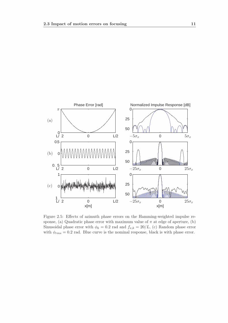
Various phase errors and their effects are illustrated in Figure 2.5 and discussed inthe following.
Phase errors that can be modeled by a polynomial of order higher than one generallycause defocusing and/or asymmetric sidelobes in the impulse response, but will not bedealt with in detail in the remainder of the report. A quadratic phase error, which canoccur if there is an uncompensated cross-track acceleration, leads to defocusing sincean incorrect azimuth chirp rate is used. Such a quadratic phase error is illustratedin Figure 2.5a. Typically, a quadratic phase error with a maximum variation of π/4along the aperture is accepted with respect to focusing quality [7].
High frequency peridodic motion errors can be modeled by a Fourier series. Con-centrating on a single sinusoidal motion error component, the azimuth phase error
2.3 Impact of motion errors on focusing 11
L/ 2 0 L/20
Phase Error [rad]
0
50
25
0Normalized Impulse Response [dB]
L/ 2 0 L/20. 5
0
0.5
0
50
25
0
L/ 2 0 L/21
0
1
x[m]0
50
25
0
x[m]
π
−5σx 5σx
−25σx
−25σx
25σx
25σx
(a)
(b)
(c)
Figure 2.5: Effects of azimuth phase errors on the Hamming-weighted impulse re-sponse, (a) Quadratic phase error with maximum value of π at edge of aperture, (b)Sinusoidal phase error with φk = 0.2 rad and fx,k = 20/L, (c) Random phase errorwith φrms = 0.2 rad. Blue curve is the nominal response, black is with phase error.
12 Motion Errors in SAR Focusing
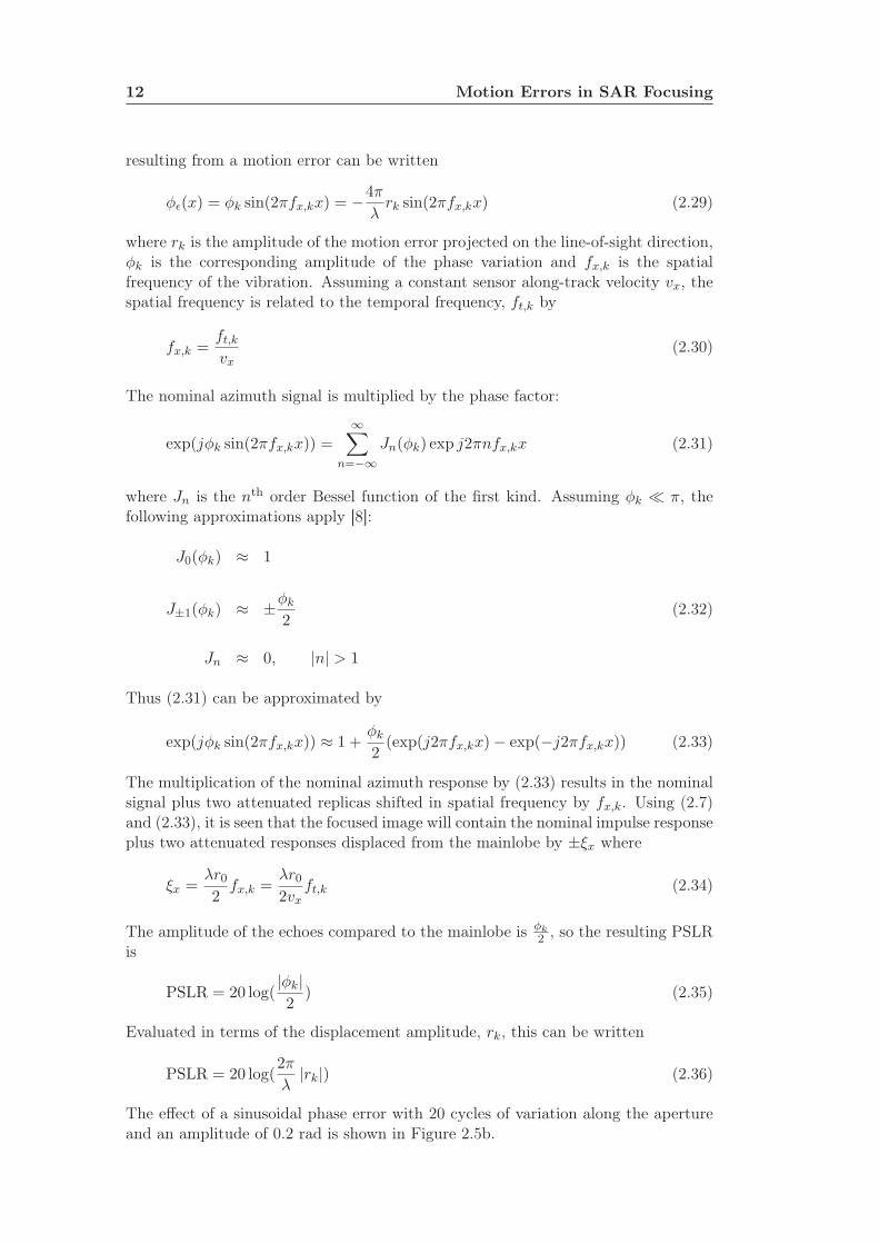
resulting from a motion error can be written
φǫ(x) = φk sin(2πfx,kx) = −4π
λrk sin(2πfx,kx) (2.29)
where rk is the amplitude of the motion error projected on the line-of-sight direction,φk is the corresponding amplitude of the phase variation and fx,k is the spatialfrequency of the vibration. Assuming a constant sensor along-track velocity vx, thespatial frequency is related to the temporal frequency, ft,k by
fx,k =ft,kvx
(2.30)
The nominal azimuth signal is multiplied by the phase factor:
exp(jφk sin(2πfx,kx)) =∞∑
n=−∞
Jn(φk) exp j2πnfx,kx (2.31)
where Jn is the nth order Bessel function of the first kind. Assuming φk ≪ π, thefollowing approximations apply [8]:
J0(φk) ≈ 1
J±1(φk) ≈ ±φk2
(2.32)
Jn ≈ 0, |n| > 1
Thus (2.31) can be approximated by
exp(jφk sin(2πfx,kx)) ≈ 1 +φk2
(exp(j2πfx,kx) − exp(−j2πfx,kx)) (2.33)
The multiplication of the nominal azimuth response by (2.33) results in the nominalsignal plus two attenuated replicas shifted in spatial frequency by fx,k. Using (2.7)and (2.33), it is seen that the focused image will contain the nominal impulse responseplus two attenuated responses displaced from the mainlobe by ±ξx where
ξx =λr02fx,k =
λr02vx
ft,k (2.34)
The amplitude of the echoes compared to the mainlobe is φk
2 , so the resulting PSLRis
PSLR = 20 log(|φk|2
) (2.35)
Evaluated in terms of the displacement amplitude, rk, this can be written
PSLR = 20 log(2π
λ|rk|) (2.36)
The effect of a sinusoidal phase error with 20 cycles of variation along the apertureand an amplitude of 0.2 rad is shown in Figure 2.5b.

2.4 Estimation of sensor motion 13
Uncorrelated random phase errors will result in sidelobes in the focused impulseresponse along the length of the aperture. The average level of these sidelobes aredetermined by the RMS-value of the phase error, and can be shown to lead to anISLR of [5]:
ISLR = 20 log(φRMS), φRMS ≪ π (2.37)
A random phase error with φRMS = 0.2 is illustrated in Figure 2.5c.
2.4 Estimation of sensor motion
For airborne SAR systems, the primary motion sensor has typically been the InertialNavigation Unit, or INU. An INU has the advantage of a high update rate (typically50-200 Hz) and high short-term accuracy, but drift of the navigation solution cancause low-frequency motion errors, with consequences for focusing as described in2.3.1. The position drift errors are typically measured in nautical miles per hour.
The Global Positioning System (GPS) complements an INU nicely, since the GPSnavigation solution has good long-term stability but a low update rate (typically onthe order of 1 Hz). Navigation systems that integrate an INU and a GPS receiverare available today, one example is the Honeywell H764G unit used in the EMISARsystem, and in the vibration analysis in Chapter 3. The accuracy of a stand-aloneGPS receiver is measured in meters, but using phase-differential methods such askinematic GPS, this can be improved to a typical accuracy of 5-10 cm. Differentialmethods require one or more reference GPS receivers on the ground. Thus applicationof kinematic GPS in on-line navigation requires real-time access to such a referencenetwork, but if this is not available, recorded navigation data can be corrected off-line.
The integration of GPS and INU navigation data is a field of study in itself, andmethods range from simple polynominal corrections of the INU data [9] to Kalmanfiltering solutions incorporating sophisticated navigation sensor models [10].


Chapter 3
Aircraft Vibrations and SAR
Focusing
In this chapter, the impact of aircraft propeller vibration on SAR focusing is ex-amined. The original motivation for this study was to examine whether the motioncompensation requirements of a high-performance SAR system – the now discontin-ued SAR++ program at Ørsted•DTU EMI [1] – could be met by a low-cost aircraftinstallation, e.g. on a propeller aircraft. As mentioned in 2.3.2, a sinusoidal motionerror causes an increase in PSLR on the focused azimuth impulse response. Onedesign goal of the SAR++ system was a Peak Sidelobe Ratio (PSLR) of −40 dBfor the impulse response. Uncompensated vibrations induced by propeller rotationcould cause undesired sidelobes in the SAR image, undermining these goals.
Previous studies of aircraft vibrations in SAR focusing have typically been carriedout in conjunction with a specific system design, e.g. [11, 12]. In these studies,the focus has been on random vibrations associated with air turbulence. However,little, if anything, has been published on high-frequency sinusoidal motion effectsfrom propeller vibration and its influence on SAR focusing. In the present study, thefocus is on high-frequency narrow-band vibrations.
For the vibration analysis, motion measurements from three different types of aircraftwere compared. The types of aircraft represent three different categories:
• A Lockheed C-130 Hercules heavy propeller transport aircraft,
• A Piper PA31 Navajo light six-seat propeller aircraft,
• A Gulfstream GIII medium-size jet aircraft, included for reference.
The three aircraft types are illustrated in Figure 3.1. The C-130 measurements arethe most complete. They were carried out by the author for the purposes of thisstudy, piggybacking on a radiometer mission over the Atlantic Ocean. The Pipermeasurements were kindly supplied by Kristian Keller of the Danish National Surveyand Cadastre (KMS), who collected them on gravimetric flights over Vadehavet inDenmark. The GIII measurements were carried out in conjunction with an EMISARflight over Zeeland, Denmark but the motion data were not used for actual SARmotion compensation.

16 Aircraft Vibrations and SAR Focusing
a)
b)
c)
Figure 3.1: Aircraft types used in vibration analysis. (a) Lockheed-Martin C130, (b)Piper Navajo PA31, (c) Gulfstream GIII.
3.1 Motion sensor description 17
l
m
n
PR
ψαw
North
West
xy
z/Up
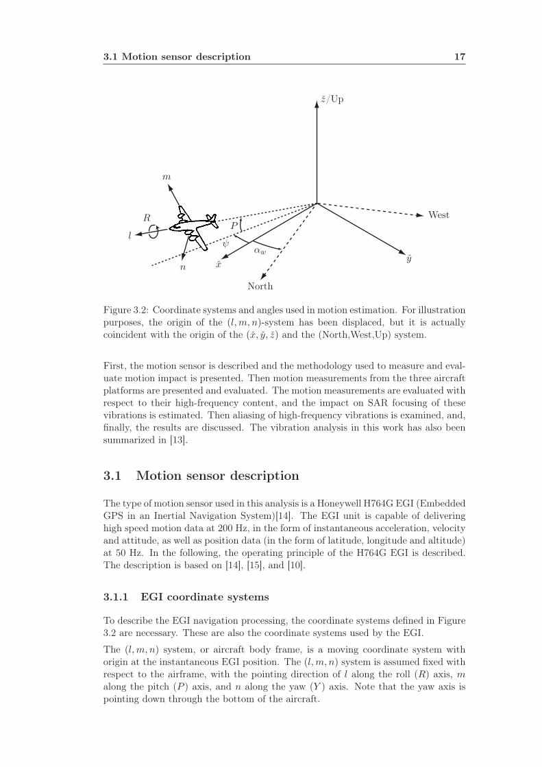
Figure 3.2: Coordinate systems and angles used in motion estimation. For illustrationpurposes, the origin of the (l,m, n)-system has been displaced, but it is actuallycoincident with the origin of the (x, y, z) and the (North,West,Up) system.
First, the motion sensor is described and the methodology used to measure and eval-uate motion impact is presented. Then motion measurements from the three aircraftplatforms are presented and evaluated. The motion measurements are evaluated withrespect to their high-frequency content, and the impact on SAR focusing of thesevibrations is estimated. Then aliasing of high-frequency vibrations is examined, and,finally, the results are discussed. The vibration analysis in this work has also beensummarized in [13].
3.1 Motion sensor description
The type of motion sensor used in this analysis is a Honeywell H764G EGI (EmbeddedGPS in an Inertial Navigation System)[14]. The EGI unit is capable of deliveringhigh speed motion data at 200 Hz, in the form of instantaneous acceleration, velocityand attitude, as well as position data (in the form of latitude, longitude and altitude)at 50 Hz. In the following, the operating principle of the H764G EGI is described.The description is based on [14], [15], and [10].
3.1.1 EGI coordinate systems
To describe the EGI navigation processing, the coordinate systems defined in Figure3.2 are necessary. These are also the coordinate systems used by the EGI.
The (l,m, n) system, or aircraft body frame, is a moving coordinate system withorigin at the instantaneous EGI position. The (l,m, n) system is assumed fixed withrespect to the airframe, with the pointing direction of l along the roll (R) axis, malong the pitch (P ) axis, and n along the yaw (Y ) axis. Note that the yaw axis ispointing down through the bottom of the aircraft.

18 Aircraft Vibrations and SAR Focusing
The (x, y, z) system is the EGI navigation frame, which the EGI uses to calculateits navigation solution. The high speed outputs (200 Hz) are also referenced to thissystem. Its origin is, as the aircraft body frame, at the instantaneous EGI position,but it is a locally level coordinate system, i.e. the x- and y-axes lie in a plane parallelto a plane that is tangent to the reference ellipsoid (the WGS-84 ellipsoid) and thez-axis is perpendicular to the reference ellipsoid and points up. The x- and y- axesare rotated relative to the North- and West-directions, respectively, by the wanderangle, αw. The wander angle is a leftover from early gimbaled INU systems. In thesesystems, the inertial sensors were isolated from aircraft movements by mountingthem in rotating gimbals, so that the sensor axes were made to physically track thenavigation frame axes. In order to prevent the sudden 180◦ change in North/Southdirection when navigating near the poles, the navigation frame axes were rotatedrelative to the North/West axes by the wander angle. The time variation of thewander angle can be described by the following expression for its derivative:
αw(t) = −ϕlon(t) · sinϕlat(t) (3.1)
The orientation of the aircraft body frame with respect to the navigation frame isgiven by the three attitude angles, ψ (azimuth angle), P (pitch), and R (roll), asdefined on the figure1. The true heading of the aircraft, ψth, can be calculated fromthe azimuth angle and the wander angle by
ψth = ψ − αw (3.2)
The coordinate transformation matrix, or direction cosine matrix, for rotating bodyframe coordinates (l,m, n) to navigation frame coordinates (x, y, z) is
Cbodynav =
CψCP −SψCR + CψSPSR SψSR + CψSPCR−SψCP −CψCR − SψSPSR CψSR − SψSPCRSP −CPSR −CPCR
(3.3)
where Cψ = cosψ, Sψ = sinψ, and so forth. Replacing ψ by ψth in (3.3) gives thecoordinate transformation from the body frame to the local geodetic frame (N,W,U).
3.1.2 EGI navigation processing
The EGI is mounted rigidly to the aircraft with its inertial sensors (accelerometersand gyros) aligned with the (l,m, n) aircraft axes. In practice, the sensor axes mayhave a different (fixed) orientation relative to the aircraft axes, but this is measuredat the time of installation and programmed into the EGI, which automatically com-pensates for this. For the purposes of the present discussion, the sensor axes can beassumed to be aligned with the (l,m, n) axes.
The inertial sensors consists of three accelerometers and three gyros. The accelerom-eters measure accelerations along the l,m, and n axes, and the gyros measure rotationrates about these axes. All measurements are with respect to inertial space.
Before a flight, the initial position and attitude of the EGI must be established.The position (latitude, longitude, and altitude) is input by the operator (or the
1Note that the term “azimuth” is often used for along-track position in SAR theory, but this isunrelated to the azimuth angle used here.

3.1 Motion sensor description 19
Figure 3.3: Inertial navigation processing flow for the H764G EGI, from [15]. Notethat the EGI used in this project uses different sampling frequencies than illustratedon the figure. Thus 1536 Hz, 256 Hz, and 64 Hz on the figure corresponds to 1200 Hz,200 Hz and 50 Hz in the EGI used in this project.
GPS position is used), after which the EGI performs an alignment to establish itsinitial attitude (azimuth, pitch, and roll angle). During the alignment, which takesa few minutes, the EGI does not move, and the pitch and roll is estimated usingthe accelerometer measurements and the fact that these only measure gravitationalacceleration when the EGI is not moving. The initial azimuth angle is establishedusing a procedure called gyrocompassing, which relies on the gyro measurementsand knowledge of the Earth rotation rate. After the alignment, the EGI can beginnavigating, as described in the following.
The processing that the EGI performs when navigating is illustrated on Figure 3.3.The inertial sensors are sampled at 1200 Hz, and the measurements are compensatedfor various non-idealities using temperature measurements and stored calibrationdata. The compensated acceleration and rotation rate measurements (∆vcomp and∆θcomp on the figure) are propagated at 200 Hz to the navigation processor (Nav1on the figure). Also, the raw measurements, filtered and decimated to 200 Hz, areavailable in the EGI output (upper left part of the figure).
As mentioned earlier, the EGI also contains a GPS receiver, which works by measur-ing the distance to GPS satellites. The EGI merges the GPS and inertial measure-ments in a Kalman filter, which uses a sophisticated model of the EGI to keep trackof various sensor errors. These include (but are not limited to) bias, scale factors,and misalignments of the inertial sensors; velocity, attitude, and position errors; andGPS clock errors. All available measurements are used in the Kalman filter, but itserror estimates are updated at 1 Hz only. Based on these error estimates, Kalmanfilter corrections are applied at all levels in the navigation processing, indicated bythe abbreviation KF in Figure 3.3. The GPS part of the EGI will not be coveredin further detail here, since it does not affect the estimate of high-frequency motionabove 1 Hz.

20 Aircraft Vibrations and SAR Focusing
After the the Kalman filter corrections for scale factors (SF), misalignment (MA)and bias of the inertial sensors, the sensor attitude is updated using the measuredattitude rates. In principle, this can be done using direction cosine matrices, butfor numerical reasons, the EGI keeps track of attitude using quarternions, which arefour-element vectors that can be used to describe rotations [10]. Mathematically,however, the results are equivalent, and in the following, the process is describedusing direction cosine matrices. The derivative of (3.3) can be written
d
dtCbodynav = Cbody
nav
0 −ωY ωPωY 0 −ωR−ωP ωR 0
(3.4)
where ωR, ωP , and ωY are the roll, pitch, and yaw axis angular rates (i.e. rotationrates about the l, m, and n axes, respectively) as measured by the gyroscopes.The attitude update (“Quarternion Update” in Figure 3.3) thus corresponds to anumerical integration of (3.4), at each step using the previous value of the storedattitude. This integration is performed at 200 Hz. Gyroscopes measure rotationsrelative to an inertial frame, but the body frame and navigation frame are bothrotating coordinate systems, so the measured attitude is corrected for the motion ofthe sensor and the Earth rate (“Transport/Earth rate” in Figure 3.3). This correction,which is combined with the Kalman filter correction of attitude, is performed on allof the 200 Hz samples, but the correction parameters are only updated at 50 Hz,since they depend on the position of the sensor, and this is only calculated at 50 Hz.
The updated, corrected attitude is used to transform the measured body frame ac-celerations to the navigation frame. Since the navigation frame is rotating, thenavigation frame accelerations include a Coriolis component, which is corrected for.The next step is the correction for the gravitational acceleration, which is calculatedusing the sensor position and a model of the Earth gravity field. The measured ac-celeration is the inertial acceleration minus the gravitational acceleration (i.e. if theEGI is sitting still on the Earth surface, it measures what appears to be an upwardsacceleration). An error in the sensor altitude will lead to an error in the estimatedgravitational acceleration, and this is a positive feedback mechanism, since if thealtitude estimate is, for example, too high, the estimated gravitational accelerationis too low, causing an upwards acceleration error. This leads to instability of thevertical position estimate, so inertial navigation units on aircraft need an externalmeasurement of altitude, which can be provided from a pressure altimeter or fromthe GPS altitude. In both cases, the external altitude measurement is merged withthe inertial measurements through the Kalman filter.
After the Coriolis and gravitational acceleration correction, the accelerations areintegrated to obtain velocities in the navigation frame (vx,y,z in Figure 3.3), andthese are available at 200 Hz. The navigation frame velocities are integrated to obtaindisplacement in the navigation frame, and this displacement is then used to updatethe sensor position (which is also the origin of the navigation frame). The positioncalculation is only performed at 50 Hz, and the output is Latitude, Longitude, andAltitude on the reference ellipsoid. The wander angle, which is used to horizontallyrotate navigation frame velocities to (North-West-Up) or (East-North-Up)-velocities,is also output at 50 Hz.
The latitude, longitude, and altitude outputs of the EGI are not suitable for SARmotion compensation, both due to coarse quantization, and due to discontinuities

3.1 Motion sensor description 21
in the data at 1 second intervals caused by the Kalman filter position corrections.Therefore, the position estimation in EMISAR processing is based on integration ofvelocities [30].
3.1.3 EGI high frequency characteristics
To use the EGI data for estimating aircraft vibration levels, the frequency charac-teristic of the EGI should be known. The EGI output sampling frequency is 200 Hz,sufficient to represent motion in the 0-100 Hz band. Unfortunately, the EGI high-frequency characteristics are not well described in the documentation, and if themeasurement bandwidth of the EGI is lower than 100 Hz, the vibration levels esti-mated from the EGI data may be lower than the actual physical vibrations. On theother hand, if the EGI measurement bandwidth extends beyond 100 Hz, vibrationsabove 100 Hz may be aliased to frequencies in the 0-100 Hz band. The followingdescription has been assembled from various references.
The accelerometers (Honeywell Q-Flex QA2000) used in the EGI have a bandwidthof more than 300 Hz [16], whereas the gyros (GG1320 Digital Ring Laser Gyro) havea bandwidth on the order of 1000 Hz when mounted in a rigid sensor block [17].According to [15], the H764 EGI’s inertial sensors are internally mounted in a rigidaluminum block, so this is indeed the case. Both values are comfortably above the100 Hz output bandwidth of the EGI, so the level of the vibrations in the band from0-100 Hz should be reliably measured by the EGI.
It is not indicated on Figure 3.3 or elsewhere in the EGI documentation whether thetransition from 1200 Hz to 200 Hz sampling implies a low-pass anti-alias filteringoperation, although this would be natural. One reason for this could be the fact thatthe gyros are dithered in order to prevent a phenomenon known as lock-in, whichcauses the output of a ring laser gyro to be 0 at low angular rates [10]. The dithering isa small amplitude, high-frequency (on the order of 500 Hz) sinusoidal rotation appliedto the gyro to ensure that it never operates in the lock-in region. It is applied insidethe gyro casing, and a piezoelectic sensor mounted in the casing estimates the applieddither, which is then subtracted before the angular rate measurement is output fromthe gyro. Nevertheless, there may be a residual dither signal present in the angularrate measurement, and this would turn up as an error peak at the dither frequency inthe spectrum of the output angular rate. If no anti-aliasing was applied, this wouldcause the dither frequency to be aliased to a frequency in the 0-100 Hz band. Thesame thing would happen to actual physical vibrations of the EGI above 100 Hz.Thus, if aliased vibration peaks can be identified in the motion data, the level of theoriginal vibration cannot be reliably estimated since the frequency characteristics ofthe EGI above 100 Hz is not known. However, the aliased motion signal will be apure error signal.
3.1.4 Selection of motion variables for vibration measurements
The output motion data that are available at 200 Hz are summarized in Table 3.1.The output raw body accelerations and angular rates are filtered, according to theupper left part of Figure 3.3), but the quantities that would be used in SAR motioncompensation are the output navigation frame velocities (vx,y,z in Figure 3.3) andnavigation frame attitude angles (not indicated directly in the Figure). On Figure 3.4

22 Aircraft Vibrations and SAR Focusing
Variable Description
al, am, an Filtered body accelerations
Y , P , R Filtered angular rates
vx, vy, vz Navigation frame velocities
ψ, P , R Azimuth angle, pitch, and roll
Table 3.1: Overview of available 200 Hz motion data.
6 6.5 7 7.5 8
0.12
0.14
0.16
Time [s]
Vel
ocity
Velocity
10-2
100
102
-40
-30
-20
-10
0
PSD Ratio, integrated a to v
Frequency [Hz]
Vel
. PS
D R
atio
n z
Int. anvz
Figure 3.4: Comparison of integrated vertical body acceleration and navigation framevertical velocity. A linear trend has been removed from both quantities.
is shown a comparison of the output navigation frame vertical velocity, vz, and thevelocity calculated from the output vertical body acceleration, an. The figure is basedon a short segment of level flight, taken from the C130 dataset described in section3.2.1. For level flight, the n and z axes are approximately parallel, although the n-axispoints down and the z-axis points up. The an component was inverted and integratedand a linear trend was removed. This was necessary since the output an has not beencompensated for gravity acceleration, but the linear trend removal does not affectthe high-frequency content. The only correction applied to vz was removal of a lineartrend. On the left side of Figure 3.4, the integrated an is plotted together with vzfor comparison. It is clearly seen that the navigation frame velocities have more highfrequency content. This is also seen from the power spectral densities (PSD) of theintegrated an and the vz components. These were calculated, and on the right partof Figure 3.4, the ratio of the two PSD’s is plotted. The ratio resembles a low-passfilter characteristic with a 3 dB frequency of 7 Hz. A similar trend was seen whencomparing output body angular rates and output navigation frame attitude angles.Although this does not reveal whether the data used in the navigation processing arelow-pass filtered, it indicates that the output body accelerations and angular ratesshould not be used for vibration level estimation since they would underestimate thehigh-frequency vibration levels seen in SAR motion compensation data above 7 Hz.
3.2 Measurements 23
3.2 Measurements
In this section, the measurement setups for the various aircraft vibration measure-ments is described.
3.2.1 C-130 measurement setup
The C-130 Hercules is a heavy military transport aircraft. As such it is not theobvious choice for a low-cost SAR installation (see the chapter introduction), asoperating cost are generally high. However, since the C-130 can fly with open doors(at low altitude) and sensor equipment can easily be installed on cargo pallets, aSAR installation could possibly be made without costly modifications of the airframe.The C-130 has four four-blade turboprop engines, and under normal operation, thepropeller rotation rate is fixed at 1020 RPM =17 Hz.
Vibration measurements for the C-130 were carried out during a radiometer flightto the North Atlantic. The H764G EGI unit used was borrowed from KMS, andfull 200 Hz velocity and attitude data were collected. Existing EGI data collectionsoftware was modified by the author for the purposes of this mission. A second EGI(the one used in EMISAR) was used by the radiometer, and on the homeward transitafter the main mission was completed, data were collected from the EMISAR EGI aswell. The EMISAR EGI has the problem, however, that attitude data are deliveredat 200 Hz but only updated at 50 Hz. This is probably due to a bug in the firmware.Velocity measurements are updated at 200 Hz, though. Unfortunately it was notpossible to collect data from both EGIs at the same time.
The KMS EGI was mounted at the bottom of a rack that was again mounted on oneof the C-130 standard cargo pallets. The installation is shown on Figure 3.5. A GPSantenna was mounted in a roof window in the front of the aircraft and connected tothe EGI to improve the long-term stability of the navigation solution, although thiswas not strictly required for the purposes of this investigation.
The data set selected for processing was collected when the C-130 was flying at analtitude of 25000 feet and a velocity of 350 knots. This velocity is close to maximumfor the C-130, which would be desirable in a SAR system to increase both flightstability and coverage. An altitude of 25000 feet was also typically intended inEMISAR flights.
3.2.2 Piper PA31 measurement setup
The Piper PA31 Navajo is a six seat light business aircraft used for many purposes.It has two three-blade turbopiston engines, where the propeller rotation rate is setby the pilot according to flight conditions and requirements. The particular aircraftused in this measurement is operated as a surveying aircraft by the Danish surveyingcompany SCANKORT A/S.
The Piper measurements were kindly supplied by Kristian Keller of the Danish Na-tional Survey and Cadastre (KMS), who collected them on gravimetry flights overVadehavet. The EGI was the same unit used for the C-130 measurements. On thePiper, the EGI was mounted in a rack that was latched into a seat mount and screwedtight to the floor. The data collection was made with software that collected only 50

24 Aircraft Vibrations and SAR Focusing
Figure 3.5: C-130 EGI Installation. The KMS EGI is indicated by the red circle andthe EMISAR EGI (yellow circle) is mounted next to it, rotated 90◦.

3.3 Vibration analysis 25
Hz data, so 200 Hz measurements are unfortunately not available.
The data set used for analysis was collected flying at 3400 feet and a speed of 150knots. However, the Piper is capable of flying at 25000 feet and a speed of 200 knots.These could be suitable values for flying a SAR system, but unfortunately motiondata were not available for these flight conditions. The maximum propeller rotationrate for the Navajo is 2575 RPM = 42.9 Hz, but the actual propeller rotation ratesused for this flight were not logged.
3.2.3 GIII measurement setup
The GIII is a medium-sized jet aircraft used for both civilian and military purposes.It has two tail-mounted turbojet engines. The EMISAR system was mounted on aGIII of the Royal Danish Airforce, and the GIII measurements were included in thisanalysis in order to compare the vibration environment of a propeller aircraft to thatof a jet aircraft.
The motion data were collected during an EMISAR flight, but not during SAR datacollection, where the EGI is controlled by EMISAR, which only collects 50 Hz data.As mentioned in 3.2.1, the EMISAR EGI only updates attitude data at 50 Hz, evenwhen 200 Hz data are collected, so only 50 Hz attitude data are available. As for themounting, the EGI was screwed tight onto a metal plate latched into a seat mount.
The flight conditions were very similar to those of the C-130 measurements, with analtitude of 25000 feet and a velocity of 380 knots.
3.2.4 Summary of flight conditions
The relevant parameters for the three different aircraft measurements are summarizedin Table 3.2
Aircraft Engine Type Speed [kts] Altitude [feet]
C-130 Hercules 4 × 4-blade Turboprop 350 25000PA-31 Navajo 2 × 3-blade Piston 150 3400Gulfstream GIII 2 × Turbojet 380 25000
Table 3.2: Flight conditions for motion measurements.
3.3 Vibration analysis
This section describes the processing carried out on the collected EGI data to esti-mate vibration amplitudes and their impact on SAR focusing.
3.3.1 Model for small aircraft vibrations
In the following, a model for small amplitude aircraft deviations from the referencetrack is derived. It is assumed that the aircraft/EGI follows a straight and leveltrack in the reference (x, y, z) coordinate system similar to Figure 2.1 and is only

26 Aircraft Vibrations and SAR Focusing
perturbed from the reference motion by small scale translational and rotational bodyvibrations. The reference motion of the SAR antenna is given by
pR(t) =
vx,nomt
00
+
1 0 00 −1 00 0 −1
dbody (3.5)
where vx,nom is the sensor reference along-track velocity and dbody is the leverarmvector from the EGI to the SAR antenna, specified in the (l,m, n) body coordinates:
dbody =
dldmdn
(3.6)
The small scale vibrations are modeled by the body accelerations, al, am, and an,and by the rotations R, P , and Y . The roll (R) and pitch (P ) angles are definedas in Figure 3.2, whereas the yaw (Y ) angle is defined like the azimuth angle, butis measured relative to the nominal track, so that a yaw angle of 0 indicates thatthe aircraft is pointed in the nominal direction of flight. According to (3.3), thetransformation from body coordinates to reference track coordinates is given by:
Cbodyref =
CY CP −SY CR + CY SPSR SY SR + CY SPCR−SY CP −CY CR − SY SPSR CY SR − SY SPCRSP −CPSR −CPCR
(3.7)
Since small perturbations are assumed, Y, P,R ≪ 1, so CX = cosX ≈ 1, andSX = sinX ≈ X, where X is either Y , P or R. With these approximations, andassuming also that double and triple products can be neglected,
Cbodyref ≈
1 −Y P
−Y −1 RP −R −1
(3.8)
The translational motion of the EGI in the (x, y, z)-system can be expressed as
pM (t) =
∫
vx,nom + vx(t)
vy(t)vz(t)
dt =
vx,nomt
00
+
∫ ∫
ax(t)ay(t)az(t)
dt2
≈
vx,nomt
00
+
∫ ∫
1 −Y (t) P (t)
−Y (t) −1 R(t)P (t) −R(t) −1
al(t)am(t)an(t)
dt2
≈
vx,nomt
00
+
∫ ∫
al(t)
−am(t)−an(t)
dt2
(3.9)
where, in the last approximation, it has been assumed that small accelerations cou-pling with small rotations can be neglected. The actual antenna motion is
pA(t) = pM (t) + Cbodyref dbody
≈ pM (t) +
1 −Y (t) P (t)
−Y (t) −1 R(t)P (t) −R(t) −1
dldmdn
(3.10)

3.3 Vibration analysis 27
The displacement from the sensor reference track caused by small scale vibrations isthen
∆p(t) ≈ pA(t) − pR(t) =
∫ ∫
al(t)
−am(t)−an(t)
dt2 +
0 −Y (t) P (t)
−Y (t) 0 R(t)P (t) −R(t) 0
dldmdn
=
∫
vx(t)vy(t)vz(t)
dt+
0 −Y (t) P (t)
−Y (t) 0 R(t)P (t) −R(t) 0
dldmdn
(3.11)
where the cross-track motion has been expressed as a function of the velocities andattitude angles, which are used in the motion estimation.
3.3.2 Estimating vibration measurement errors
When estimating the impact of vibrations on the SAR impulse response, it is im-portant to note that it is not the vibrations themselves that cause phase errors, butthe failure to estimate and compensate them correctly. The motion measurementspresented in this chapter were carried out with one motion sensor, and so a “truth”value is not available for comparison. Ideally, two motion sensors should have beenused simultaneously, but this was unfortunately not possible. However, the under-lying assumption in the following is that the estimate of high frequency motion dueto vibration is potentially erroneous. There are several reasons why the vibrationcontent of measured motion data might not correspond to the actual motion of theSAR antenna:
1. High frequency vibrations can be due to structural vibrations in the airframe.If the SAR antenna is displaced from the motion sensor, the amplitude and/orphase of the vibration might be different at the two locations. This phenomenonis referred to as leverarm flexure. Leverarm flexure effects can be reduced bymounting the motion sensor close to the SAR antenna, but this might not bepossible in a low-cost installation.
2. For high frequency vibrations, small unknown delays between SAR data andmotion data will cause a frequency-dependent phase shift of the measured vi-bration. For example, a 10 ms delay will cause a 50 Hz vibration to be measured180◦ out of phase, doubling the motion induced phase error. Delays betweenSAR data and motion data can of course be reduced by proper design and cal-ibration of the SAR system and motion sensor, but it is necessary to be awareof this.
3. High frequency vibrations that are undersampled by the motion sensor canturn up at a lower aliased frequency. Since SAR data are typically collected ata higher frequency than motion data, the corresponding vibration componentin the SAR data might not be aliased at all or aliased to a different frequency.This means that, in addition to the uncompensated vibration in the SAR data,a new vibration component is introduced by the motion compensation at thealiased frequency. Means to reduce aliasing effects include using a motionsensor with higher sampling frequency, but systems with a sampling frequencyhigher than 300 Hz are not generally available.

28 Aircraft Vibrations and SAR Focusing
Aliasing effects can to some extent be identified in the motion sensor data if it isrelated to harmonics of the propeller frequency. For the other two types of errorthe motion error cannot be predicted, but it is likely that the potential motionerror induced would be the same order of magnitude as the measured vibrations.Therefore, measuring the actual vibration environment provides a rough estimate ofthe magnitude of such errors.
3.3.3 Assumed SAR system description
To evaluate the impact of measured vibration levels on SAR focusing, assumptionsregarding the SAR system must be made. As mentioned in the chapter introduction,the work was carried out with the SAR++ system [1] in mind. This work consid-ered both L, C, and X-band systems. The sidelobes introduced by vibrations will belargest for an X-band system, since according to (2.36) the PSLR is inversely propor-tional to wavelength, and furthermore, an X-band system will generally have smallerphysical dimensions than lower-frequency systems, which would make an installationon a small aircraft more feasible. Therefore the system parameters from the SAR++X-band configurations have been adopted. The relevant parameters assumed for thevibration analysis are summarized in Table 3.3. The assumed sensor velocity andaltitude are those used in each individual motion measurement (see Table 3.2).
Parameter Value
Wavelength, λ 3.2 cmUnweighted azimuth resolution 0.25 mLook angle, θR 45◦
Table 3.3: Assumed SAR system parameters for analysis.
3.3.4 Motion data processing
In order to get results that are meaningful in a SAR context, the EGI data describedin section 3.1.4 must first be transformed to a suitable SAR imaging coordinatesystem. Thus, short data sets (of a few minutes) exhibiting approximately constantcourse, velocity and altitude (i.e. during transit) were selected. Since the variationof the wander angle is slow when not travelling near the poles, it is assumed constantfor the short duration being processed (see also (3.1)). The mean of the wander anglewill be accounted for by the procedure described below, and the actual discrepancyin impulse response arising from assuming a constant wander angle will be of a low-frequency nature, and thus insignificant in the context of this investigation. Theinvestigation proceeds as follows, using the measure motion data summarized inTable 3.1:
1. Select anN -sample motion data set of approximately constant heading, velocityand altitude.
2. Calculate dataset mean of horizontal velocity vector components, i.e the navi-gation frame velocities vx[1 : N ] and vy[1 : N ].
3.3 Vibration analysis 29
3. Calculate dataset mean azimuth angle by
ψmean = − arctan(vy,mean/vx,mean)
Note that ψ is measured positive clockwise with respect to the x-axis.
4. Calculate the yaw angle, Y by:
Y [1 : N ] = ψ[1 : N ] − ψmean
5. Rotate horizontal velocities to the SAR imaging coordinate system by
vxvyvz
=
cos(ψmean) sin(ψmean) 0− sin(ψmean) cos(ψmean) 0
0 0 1
vxvyvz
After this preprocessing, estimates of along-track velocity, vx, across-track velocities,vy and vz, and attitude angles Y , P , and R are available.
The spectra of the measured motion data are estimated by the Welch power spectrumestimation method [18]. With this method, N data samples are divided into smallerbins of length L, with an overlap, M , between bins. Each bin is windowed by asuitable window function (a Blackman window in this work), transformed by FFT,and the resulting amplitude spectra are averaged over all bins. This method waschosen for its simplicity.
The output of the spectral analysis is power spectral density (PSD), which is mea-sured in (m/s)2/Hz for velocities and rad2/Hz for attitude angles. Sinusoidal vi-brations will turn up as more or less well-defined peaks in the power spectra, andthe power in one peak can be estimated by integrating the power spectrum over thewidth of the peak. This estimated power, Γk, can again be converted to a sinuoidalamplitude, Ak:
Ak =
√2 · Γk (3.12)
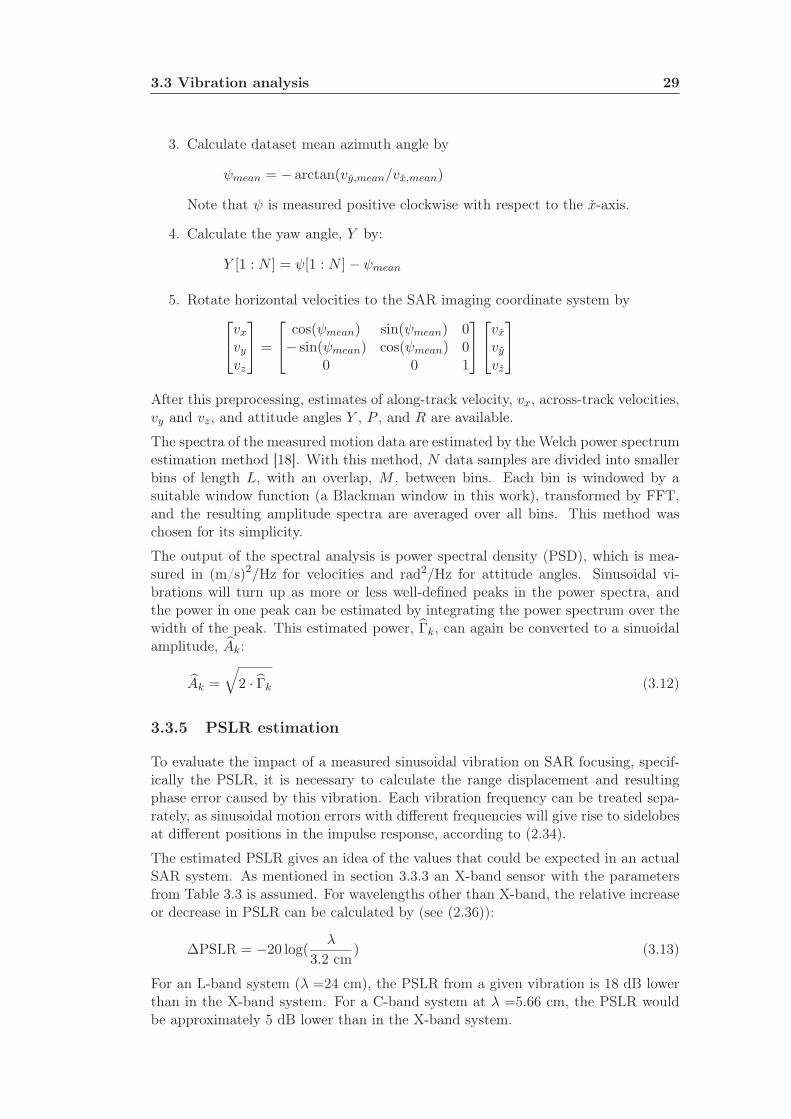
3.3.5 PSLR estimation
To evaluate the impact of a measured sinusoidal vibration on SAR focusing, specif-ically the PSLR, it is necessary to calculate the range displacement and resultingphase error caused by this vibration. Each vibration frequency can be treated sepa-rately, as sinusoidal motion errors with different frequencies will give rise to sidelobesat different positions in the impulse response, according to (2.34).
The estimated PSLR gives an idea of the values that could be expected in an actualSAR system. As mentioned in section 3.3.3 an X-band sensor with the parametersfrom Table 3.3 is assumed. For wavelengths other than X-band, the relative increaseor decrease in PSLR can be calculated by (see (2.36)):
∆PSLR = −20 log(λ
3.2 cm) (3.13)
For an L-band system (λ =24 cm), the PSLR from a given vibration is 18 dB lowerthan in the X-band system. For a C-band system at λ =5.66 cm, the PSLR wouldbe approximately 5 dB lower than in the X-band system.

30 Aircraft Vibrations and SAR Focusing
In the following, each component of the measured vibrations (vy, vz, Y , P , R) isanalyzed individually (vx does not give rise to significant range displacement, seesection 2.2.1). A line-of-sight look angle of θR = 45◦ is assumed, as mentioned inTable 3.3. This is a typical look-angle for an airborne SAR.
According to (3.11) and (2.15), a horizontal cross-track velocity vibration of frequencyft,k and amplitude vy,k will be projected on to the line-of-sight direction (θ = 45◦),and give rise to the range displacement ∆ry,k:
∆ry,k = sin θR
∫vy,k sin(2πft,kt)dt = − vy,k
2√
2πft,kcos(2πft,kt) (3.14)
Likewise, a vertical velocity vibration of amplitude vz,k will give a range displacement
∆rz,k = − cos θR
∫vz,k sin(2πft,kt)dt =
vz,k
2√
2πft,kcos(2πft,kt) (3.15)
The estimated range displacement amplitude is then, for both a horizontal and avertical cross-track velocity:
∆rv,k =vk
2√
2πft,k(3.16)
The effect of angular vibration can also be seen from (3.11), assuming straight andlevel flight for which Y, P,R≪ 1. Looking at the cross-track components (only theygive rise to range displacements), the range displacement is
∆rΘ,k =
[−Y dl +RdnPdl −Rdm
]· nT
= (−Y dl +Rdn) sin θR − (Pdl −Rdm) cos θR (3.17)
The resulting displacement is highly dependent on the leverarm chosen. Since thereis no “right” way to chose this, the displacement amplitude corresponding to a specificangular parameter will be estimated by multiplying the vibration amplitude by 1 m.This isolates the effect of a vibration in a single attitude parameter, and gives a resultthat can be easily related to other leverarm sizes.
To sum up, the following expression can be used to evaluate the PSLR resulting froma velocity vibration of amplitude vk and frequency ft,k (see (2.36) and (3.16)):
PSLRv =φk2
=vk√
2λft,k(3.18)
The PSLR from an angular vibration of amplitude Θk is estimated as
PSLRΘ =
√2π
λdΘΘk (3.19)
with Θk given in radians, dΘ = 1 m and the displacement projected on the 45◦
line-of-sight direction.

3.4 C-130 measurements 31
3.4 C-130 measurements
3.4.1 Motion spectra
The collected motion data for the C-130 were processed as described in section 3.3.4.The estimated vibration spectra are shown in Figures 3.6 and 3.7. A Blackmanwindow was used in the power spectrum estimation to decrease leakage, especiallyfrom the low-frequency part of the motion spectrum, which is typically of much largermagnitude than the high-frequency part. The selected values of N , L, and M in thepower spectrum estimation (see section 3.3.4), were a compromise between having along enough data set for sufficient resolution and noise reduction and a sufficientlyshort data set for constant flight conditions. At the 200 Hz sampling rate, N = 10000corresponds to 50 seconds of data.
Examining the high-frequency part (>10 Hz) of the vy spectrum, a relatively constantnoise floor with peaks at the frequencies 17, 34, 51, 68, and 85 Hz is seen. The C-130 uses constant-speed 4-blade propellers rotating at 1020 RPM or 17 Hz, so themeasured frequencies are the fundamental and higher harmonics of the propellerfrequency. The largest peak is actually at the blade frequency, 68 Hz, and not at thefundamental propeller frequency. The noise floor level is consistent with the nominalRMS jitter of the EGI velocity outputs [14]. This is specified as 6 · 10−4 m/s, givinga single sided noise density of −84 dB/Hz with 200 Hz sampling.
The vz spectrum looks similar to the vy spectrum except for a slight increase in thenoise floor between 50 Hz and 60 Hz, the cause of which is not known. Also, a smallpeak is seen at 64 Hz which is consistent with the second harmonic(=136 Hz) of theblade frequency aliased by the 200 Hz sampling.
Looking at the attitude spectra, there is an average noise floor slightly below −110 dB/Hz,which is probably due to the EGI attitude quantization of 96 µrad, giving a quan-tization noise density of -114 dB/Hz. The strongest vibration peak is seen at thefundamental harmonic of the blade frequency, 68 Hz, and the second strongest at thealiased second blade harmonic at 64 Hz. Both peaks are strongest in the roll anglespectrum.
To sum up, the vibration amplitudes estimated from the motion spectra are given inTable 3.4. The table allows a comparison of the different vibration components butdo not directly say anything about their impact on SAR focusing. This is analyzedin the following section.
Frequency vx vy vz R P YHz mm/s mm/s mm/s µrad µrad µrad
17 0.3 1.5 2.7 6.9 8.5 0.034 0.2 0.8 0.5 4.7 3.0 1.051 0.5 0.4 1.7 2.5 9.2 0.564 0.1 0.0 0.2 36.9 13.1 8.868 3.3 7.5 4.3 51.8 22.6 7.385 0.1 0.2 0.2 2.7 0.0 1.2
Table 3.4: C-130 measured vibration amplitudes.

32 Aircraft Vibrations and SAR Focusing
0 20 40 60 80 100−100
−80
−60
−40
−20
v
PS
D [1
0log
10{(
m/s
)2 /Hz}
]
0 20 40 60 80 100−100
−80
−60
−40
−20
v
PS
D [1
0log
10{(
m/s
)2 /Hz}
]
0 20 40 60 80 100−100
−80
−60
−40
−20
v
Frequency [Hz]
PS
D [1
0log
10{(
m/s
)2 /Hz}
]
x
y
z
Int.
Figure 3.6: C-130 Power spectral densities (PSD) for velocities. N=10000, L=1024,M=512, Blackman window.

3.4 C-130 measurements 33
0 20 40 60 80 100−120
−110
−100
−90
−80
−70
−60Roll
PS
D [1
0log
10{(
rad)
2 /Hz}
]
0 20 40 60 80 100−120
−110
−100
−90
−80
−70
−60Pitch
PS
D [1
0log
10{(
rad)
2 /Hz}
]
0 20 40 60 80 100−120
−110
−100
−90
−80
−70
−60Yaw
Frequency [Hz]
PS
D [1
0log
10{(
rad)
2 /Hz}
]
Figure 3.7: C-130 Power spectral densities (PSD) for attitude angles. N=10000,L=1024, M=512, Blackman window.
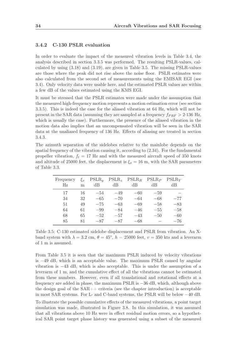
34 Aircraft Vibrations and SAR Focusing
3.4.2 C-130 PSLR evaluation
In order to evaluate the impact of the measured vibration levels in Table 3.4, theanalysis described in section 3.3.5 was performed. The resulting PSLR-values, cal-culated by using (3.18) and (3.19), are given in Table 3.5. The missing PSLR-valuesare those where the peak did not rise above the noise floor. PSLR estimates werealso calculated from the second set of measurements using the EMISAR EGI (see3.4). Only velocity data were usable here, and the estimated PSLR values are withina few dB of the values estimated using the KMS EGI.
It must be stressed that the PSLR estimates were made under the assumption thatthe measured high-frequency motion represents a motion estimation error (see section3.3.5). This is indeed the case for the aliased vibration at 64 Hz, which will not bepresent in the SAR data (assuming they are sampled at a frequency fPRF > 2·136 Hz,which is usually the case). Furthermore, the presence of the aliased vibration in themotion data also implies that an uncompensated vibration will be seen in the SARdata at the unaliased frequency of 136 Hz. Effects of aliasing are treated in section3.4.3.
The azimuth separation of the sidelobes relative to the mainlobe depends on thespatial frequency of the vibration causing it, according to (2.34). For the fundamentalpropeller vibration, ft = 17 Hz and with the measured aircraft speed of 350 knotsand altitude of 25000 feet, the displacement is ξx = 16 m, with the SAR parametersof Table 3.3.
Frequency ξx PSLRy PSLRz PSLRR PSLRP PSLRY
Hz m dB dB dB dB dB
17 16 −54 −49 −60 −59 −34 32 −65 −70 −64 −68 −7751 49 −75 −63 −69 −58 −8364 61 −99 −84 −46 −55 −5868 65 −52 −57 −43 −50 −6085 81 −87 −87 −68 − −76
Table 3.5: C-130 estimated sidelobe displacement and PSLR from vibration. An X-band system with λ = 3.2 cm, θ = 45◦, h = 25000 feet, v = 350 kts and a leverarmof 1 m is assumed.
From Table 3.5 it is seen that the maximum PSLR induced by velocity vibrationsis −49 dB, which is an acceptable value. The maximum PSLR caused by angularvibration is −43 dB, which is also acceptable. This is under the assumption of aleverarm of 1 m, and the cumulative effect of all the vibrations cannot be estimatedfrom these numbers. However, even if all translational and rotational effects at afrequency are added in phase, the maximum PSLR is −36 dB, which, although abovethe design goal of the SAR++ criteria (see the chapter introduction) is acceptablein most SAR systems. For L- and C-band systems, the PSLR will be below −40 dB.
To illustrate the possible cumulative effects of the measured vibrations, a point targetsimulation was made, illustrated in Figure 3.8. In this simulation, it was assumedthat all vibrations above 10 Hz were in effect residual motion errors, so a hypothet-ical SAR point target phase history was generated using a subset of the measured

3.4 C-130 measurements 35
Figure 3.8: Point target simulation with the assumption that all motion above 10 Hzis a residual motion error.
motion data, (vx, vy, vz, Y, P,R), low-pass filtered to a 10 Hz bandwidth. The cho-sen subset corresponds to the length of a single aperture, with the SAR parametersfrom Table 3.3. This simulated signal history was then phase corrected using thenon-filtered version of the motion data and focused. In this way, the measuredmotion signal above 10 Hz is interpreted as motion estimation error. A leverarm,dbody = (1/
√3 m, 1/
√3 m, 1/
√3 m)T , was assumed, since in a high-vibration envi-
ronment, a short distance between motion sensor and SAR antenna is critical [20].The resulting impulse response can be seen on Figure 3.9. It is seen from the figurethat the simulated PSLR is below −40 dB for all sidelobes, with the two largestpairs at −42 dB and −45 dB. These are due to the 68 Hz and 64 Hz (136 Hz aliased)vibrations, respectively, and caused by the roll angular vibration working throughthe leverarm. If instead a leverarm d = (1/
√3 m, 1/
√3 m,−1/
√3 m)T is selected
these two peaks are reduced by more than 10 dB. This is in agreement with (3.17),since cos(45◦) = sin(45◦).
Summing up, the effects of the measured C-130 vibrations on the SAR impulseresponse seem to be within acceptable limits, i.e. below −40 dB. It can be brieflynoted that sidelobes consistent with a 17 Hz-vibration have actually been seen infocused SAR data acquired from a C-130 [19, 20]. This was in an X-band system,and the sidelobe level was within the acceptable limits.
3.4.3 Aliasing of motion data
Ideally, the motion sensor input bandwidth (e.g. physical gyro or accelerometerbandwidth) should be less than or equal to half the INU sampling rate to avoidaliasing. In this case, the residual motion error resulting from an out-of-band vibra-tion would only be the actual physical vibration seen in the SAR data. However, aswas seen in section 3.4.1, a high-frequency motion signal can be aliased to a lowerfrequency due to the motion sensor sampling. Since the EGI measures translationalaccelerations and rotational attitude rates, accelerations must be integrated twiceto obtain displacement, and attitude rates integrated once to obtain attitude. Anacceleration sinusoidal component ak at frequency ft,k gives rise to a displacement

36 Aircraft Vibrations and SAR Focusing
−100 −50 0 50 100−80
−70
−60
−50
−40
−30
−20
−10
0N
orm
aliz
ed A
mpl
itude
[dB
]
Azimuth [m]
Figure 3.9: Simulated C-130 azimuth impulse response with vibration errors.
given by:
yk =
∫ ∫akcos(2πft,kt)dt
2 = −akcos(2πft,kt)(2πft,k)2
(3.20)
If the acceleration signal is undersampled so that ft,k is aliased to fA, the displace-ment estimated from the motion data is:
yA =
∫ ∫akcos(2πfAt)dt
2 = −akcos(2πfAt)(2πfA)2
(3.21)
The aliased signal amplitude, yA, is larger than the amplitude of the original signalby a factor of (ft,k/fA)2. Likewise, aliasing of the attitude rate signal or the velocitysignal leads to an increase in amplitude of (ft,k/fA). Thus, an in itself insignificantout-of-band vibration can, through aliasing, result in an error signal of significantlylarger amplitude than the unaliased signal. This could lead to unacceptable sidelobelevels. However, the highest sidelobe levels will also be associated with the lowestaliased frequency. If the aliased vibration period becomes longer than the syntheticaperture duration, the sidelobes will fall within the mainlobe. In this case, the phaseerror should be treated as a low-frequency phase error (see section 2.3.1).
To illustrate the potential effects of aliasing, it is examined what happens if the EGI50 Hz data are used for motion compensation instead of 200 Hz data. This excerciseis not purely hypothetical, since for example EMISAR collects only the EGI 50 Hzdata for SAR focusing. It is important to note here, that the EGI integrates rotationrates and accelerations internally at 200 Hz. Attitude rates and accelerations in theband from 0-100 Hz will thus be integrated correctly to obtain attitude and velocity.However, the integration of velocity to obtain position will be performed at 50 Hz,causing aliasing of vibrations above 25 Hz. This could be avoided if the 50 Hz EGI
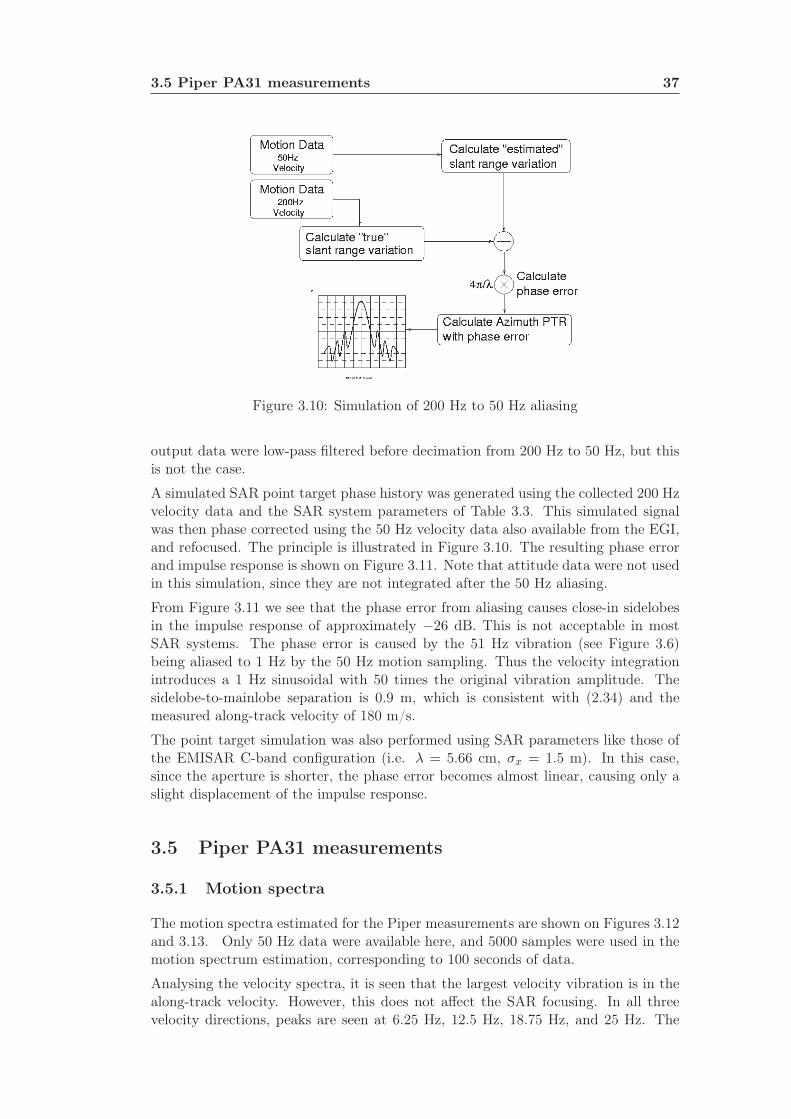
3.5 Piper PA31 measurements 37
Figure 3.10: Simulation of 200 Hz to 50 Hz aliasing
output data were low-pass filtered before decimation from 200 Hz to 50 Hz, but thisis not the case.
A simulated SAR point target phase history was generated using the collected 200 Hzvelocity data and the SAR system parameters of Table 3.3. This simulated signalwas then phase corrected using the 50 Hz velocity data also available from the EGI,and refocused. The principle is illustrated in Figure 3.10. The resulting phase errorand impulse response is shown on Figure 3.11. Note that attitude data were not usedin this simulation, since they are not integrated after the 50 Hz aliasing.
From Figure 3.11 we see that the phase error from aliasing causes close-in sidelobesin the impulse response of approximately −26 dB. This is not acceptable in mostSAR systems. The phase error is caused by the 51 Hz vibration (see Figure 3.6)being aliased to 1 Hz by the 50 Hz motion sampling. Thus the velocity integrationintroduces a 1 Hz sinusoidal with 50 times the original vibration amplitude. Thesidelobe-to-mainlobe separation is 0.9 m, which is consistent with (2.34) and themeasured along-track velocity of 180 m/s.
The point target simulation was also performed using SAR parameters like those ofthe EMISAR C-band configuration (i.e. λ = 5.66 cm, σx = 1.5 m). In this case,since the aperture is shorter, the phase error becomes almost linear, causing only aslight displacement of the impulse response.
3.5 Piper PA31 measurements
3.5.1 Motion spectra
The motion spectra estimated for the Piper measurements are shown on Figures 3.12and 3.13. Only 50 Hz data were available here, and 5000 samples were used in themotion spectrum estimation, corresponding to 100 seconds of data.
Analysing the velocity spectra, it is seen that the largest velocity vibration is in thealong-track velocity. However, this does not affect the SAR focusing. In all threevelocity directions, peaks are seen at 6.25 Hz, 12.5 Hz, 18.75 Hz, and 25 Hz. The

38 Aircraft Vibrations and SAR Focusing
−400 −300 −200 −100 0 100 200 300 400−20
−10
0
10
Azimuth [m]
Pha
se E
rror
[deg
]
−3 −2 −1 0 1 2 3−60
−40
−20
0
Nor
mal
ized
Am
plitu
de [d
B]
Azimuth [m]
Figure 3.11: Phase error and impulse response with aliasing for an X-band systemwith 25 cm azimuth resolution. Blue curve is impulse response with no phase error.
shape of the 6.25 Hz and 12.5 Hz peaks suggest that they are actually several peakswith narrow spacing, indicating aliasing. For the attitude measurements, the pitchparameter shows the strongest peaks, whereas there is only a very weak 12.5 Hz peakin the yaw parameter. Also in the attitude parameters, the 6.25 Hz and 12.5 Hz peaksseem to actually be several peaks. It was attempted to separate the peaks by usinga longer data window in the power spectrum estimation, but this did not succeed.
Above 5 Hz, the noise floor in the velocity spectra is located at approximately−75 dB/Hz. This is 3 dB higher than expected from the EGI nominal velocity jitter(see section 3.4.1), which is equivalent to a single-sided noise density of −78 dB/Hzwith the 50 Hz sampling. For the attitude parameters, the quantization noise has asingle sided density of −105 dB/Hz which is in agreement with the observed attitudespectra.
The peak positions are most likely related to the propeller RPM, but since this isnot known, guesses must be made. This is complicated by the fact that the EGIoperates internally at 200 Hz. Thus, a vibration above 100 Hz will be aliased firstby the 200 Hz sampling. If the aliased vibration frequency falls above 25 Hz, it willagain be aliased by the 50 Hz sampling of the EGI output data that has been usedin the PA31 measurements. Comparing the observed frequencies with the typicalRPM operating range for the Piper PA31, the most likely propeller rate candidatesare 1875 RPM=31.25 Hz, or 2625 RPM=43.75 Hz. Of these, the former is themost likely, since the specified maximum continuous operating RPM for the Piperis 2575 RPM. Also, the low RPM is consistent with the fact that the measurementswere taken at a speed well below the maximum cruise speed (150 knots comparedto 200 knots). With an RPM of 1875 and the aliasing described above, the aliased

3.5 Piper PA31 measurements 39
0 5 10 15 20 25−90
−80
−70
−60
−50
−40
v
PS
D [1
0log
10{(
m/s
)2 /Hz}
]
0 5 10 15 20 25−90
−80
−70
−60
−50
−40
v
PS
D [1
0log
10{(
m/s
)2 /Hz}
]
0 5 10 15 20 25−90
−80
−70
−60
−50
−40
v
Frequency [Hz]
PS
D [1
0log
10{(
m/s
)2 /Hz}
]
x
y
z
Figure 3.12: Piper PA31 power spectral densities (PSD) for velocities. N=5000,L=1024, M=512, Blackman window.

40 Aircraft Vibrations and SAR Focusing
0 5 10 15 20 25−120
−110
−100
−90
−80
−70
−60Roll
PS
D [1
0log
10{(
rad)
2 /Hz}
]
0 5 10 15 20 25−120
−110
−100
−90
−80
−70
−60Pitch
PS
D [1
0log
10{(
rad)
2 /Hz}
]
0 5 10 15 20 25−120
−110
−100
−90
−80
−70
−60Yaw
Frequency [Hz]
PS
D [1
0log
10{(
rad)
2 /Hz}
]
Int.
Figure 3.13: Piper PA31 power spectral densities (PSD) for attitude. N=5000,L=1024, M=512, Blackman window.

3.5 Piper PA31 measurements 41
propeller harmonics will be located at the frequencies in Table 3.6. The 8th harmonicwill be aliased to 0 Hz, so it will not be discernible from the non-aliased low-frequencymotion.
Frequency [Hz] Harmonics Aliased to Frequency
6.25 3rd (93.75 Hz) & 5th (156.25 Hz)12.5 2nd (62.5 Hz) & 6th (187.5 Hz)18.75 Fundamental (31.25 Hz), 7th (218.75 Hz) & 9th (281.25 Hz)25.0 4th (125 Hz)
Table 3.6: Aliased harmonics of PA31 propeller frequency at 1875 RPM. The har-monics have been aliased first by 200 Hz sampling and then by 50 Hz sampling.
The shape of the 6.25 Hz and 12.5 Hz peaks are explained by the fact that twoharmonics actually alias to those frequencies. Also, the 3rd and 6th harmonics are thefundamental and second harmonics of the blade frequency, since the PA31 has three-blade propellers. In the C-130 data, the strongest peaks were observed at the bladefrequency in both the velocity and attitude data. If this was the case here, the largestpeak should be at 6.25 Hz. The reason that the 12.5 Hz peak is the largest is probablythat the 6th harmonic (=second blade harmonic) is aliased to 12.5 Hz already in theinitial 200 Hz sampling before acceleration integration. The fundamental and 3rd
blade harmonics are acceleration-integrated at 93.75 Hz (unaliased) and 81.25 Hz(aliased) respectively. The higher frequency leads to relatively smaller amplitudes ofthe integrated acceleration vibrations (see section 3.4.3).
3.5.2 PA31 PSLR Evaluation
Since all the peaks are aliased and some fall close to each other, it is difficult toestimate the power content of the individual peaks. If close-lying peaks are treatedas one peak, the vibration amplitudes in Table 3.7 are observed. Converting thevibration amplitudes to PSLR (see sections 3.3.5 and 3.4.2), the results in Table 3.8are seen.
Frequency vx vy vz R P YHz mm/s mm/s mm/s µrad µrad µrad
6.25 0.3 1.0 1.4 9.0 21.5 0.012.50 2.5 1.5 1.0 24.9 191.9 4.618.75 1.6 0.9 0.3 16.2 20.6 2.4
Table 3.7: PA31 measured vibration amplitudes
We see here that the only critical vibration is the angular vibration in the pitchparameter aliased to 12.5 Hz. This leads to a PSLR of −31 dB if working througha 1 m leverarm component. This is larger than the design goal of −40 dB in theSAR++ requirements (see the chapter introduction). If the 200 Hz motion data wereused, the fundamental, 2nd, and 3rd propeller harmonics would not be aliased, but the6th propeller harmonic would still be aliased to 12.5 Hz. Thus, if a significant part ofthe power seen in the 12.5 Hz peak in the pitch spectrum comes from the aliased 6th

42 Aircraft Vibrations and SAR Focusing
Frequency ξx PSLRy PSLRz PSLRR PSLRP PSLRY
Hz m dB dB dB dB dB
6.25 1.9 −49 −46 −58 −51 −12.50 3.8 −51 −55 −49 −31 −6418.75 5.7 −60 −68 −53 −51 −70
Table 3.8: PA31 estimated sidelobe displacement and PSLR from vibration. AnX-band system with λ =3.2 cm, θ = 45◦, h=1000 m, and a leverarm of 1 m isassumed.
propeller harmonic, there could still be unacceptable sidelobes at ξx = 3.8 m withthe given system parameters and leverarm. To illustrate the possible cumulativeeffects of these aliased vibrations, a point target simulation similar to the one insection 3.4.2 was made. The SAR parameters used were the same as in the C-130measurement, except that an altitude of 1000 m and a velocity of 150 knots wasassumed, as the vibration data were acquired under these flight conditions. Thesimulated phase history was generated using the motion data low-pass filtered to a5 Hz bandwidth, but phase corrected by the non-filtered motion data before focusing.The resulting impulse response is presented on Figure 3.14. Here it is seen that thePSLR associated with the 12.5 Hz peak is −32 dB, whereas the cumulative effectsof the 6.25 Hz vibrations amount to a PSLR of −37 dB.
−10 −5 0 5 10−80
−70
−60
−50
−40
−30
−20
−10
0
Nor
mal
ized
Am
plitu
de [d
B]
Azimuth [m]
z
Figure 3.14: Simulated PA31 azimuth impulse response with vibration errors.
In estimating the PSLR values of Table 3.8 and Figure 3.14, it was assumed that the50 Hz motion data are used for motion compensation, unfiltered. With the 50 Hzsampling, all of the observed motion signal above 5 Hz is actually aliased and canbe removed by a low-pass filter. Harmonics that are aliased to low frequencies where

3.6 Gulfstream GIII measurements 43
there is already physical motion (e.g. the 8th harmonic aliased to 0 Hz), however,cannot be filtered this way. Either way, the actual physical vibrations will be leftuncompensated, and cause sidelobes in the SAR data. Their level, however, willlikely be equal to or smaller than the levels seen in Table 3.8 (See also section 3.4.3).
3.6 Gulfstream GIII measurements
3.6.1 Motion spectra
For reference, motion spectra for a Gulfstream GIII jet aircraft are also presentedhere. They were acquired during an EMISAR flight with the EMISAR EGI. Themotion measurements were processed the same way as for the C-130 measurements(see section 3.4.1), and the resulting spectra are shown on Figures 3.16 and 3.17. Asmentioned in section 3.2.1, due to a bug, the EMISAR EGI only updates attitudedata at 50 Hz, even in the 200 Hz data. Therefore, Figure 3.17 only shows theattitude spectrum up to 25 Hz. However, the velocity spectrum of Figure 3.16 canbe directly compared to the C-130 velocity spectrum on Figure 3.6. It is clear thatthere are no signifcant vibration peaks in the GIII spectra compared to the C-130spectra. The attitude parameters, especially, show only a noise floor above a few Hz.This noise floor is consistent with the expected quantization noise density of -105dB/Hz.
A PSLR-evaluation was not made for the GIII data due to the low observed vibrationlevels. However, a point target simulation, similar to the one in section 3.4.2 wasmade. The assumed SAR system parameters were the same as for the C-130 case, butonly velocity data were used. This is because the attitude data were only availableat 50 Hz, and furthermore, as seen from Figure 3.17, there does not appear to beany angular motion signal above a few Hz. The simulated phase history was, as forthe C-130 point target simulation, generated using the motion data low-pass filteredto a 10 Hz bandwidth but phase corrected using the non-filtered motion data. Thesimulated impulse response is seen on Figure 3.15. It is seen that there are practicallyno discernable sidelobes.
3.7 Discussion
From the analysis in the preceding section it seems clear that the actual propeller-induced cross-track vibrations - which will appear as small sinusoidal variations inthe SAR signal phase - will not lead to unacceptable sidelobes if left uncorrected.This is under the assumption of a small leverarm of less than 1 m between motionsensor and SAR antenna. If the motion sensor sampling frequency is too low, high-frequency vibrations might be aliased to lower frequencies before integration in theINU, and this will result in spurious vibrations in the motion data not reflected by theSAR data. That is worse, since the integration of the aliased sinuosidal is performedat a lower frequency. This will in turn lead to a higher level of the spurious signalcompared to the signal that caused it. Ideally, the INU should perform anti-aliasfiltering on its sensor inputs, which could be achieved by an initial oversamplingand digitial filtering of the acceleration and gyro outputs. Actually, as describedin section 3.1.2, the sensor signals are initially oversampled by a factor of 6 (i.e.

44 Aircraft Vibrations and SAR Focusing
−100 −50 0 50 100−80
−70
−60
−50
−40
−30
−20
−10
0N
orm
aliz
ed A
mpl
itude
[dB
]
Azimuth [m]
Figure 3.15: GIII Simulated impulse response with vibration errors.
1200 Hz), but aliasing was seen in the 200 Hz C-130 data, indicating that aliasing isnot fully suppressed internally in the EGI. It is also clear that the 50 Hz velocitiesoutput together with position data are not lowpass-filtered before decimation from200 Hz. This suggests that for propeller aircraft systems, the full bandwidth shouldbe used. As was shown in 3.4.3, the C-130 has a propeller harmonic of 51 Hz, whichwill alias to 1 Hz if the 50 Hz motion data are used. The resultant sidelobes seem notto be significant for L- and C-band systems as they fall in the mainlobe. Howeverfor a 25 cm resolution X-band system, the sidelobes will separate from the mainlobe,deteriorating the image quality, as illustrated in Figure 3.11.
For the PA31 Navajo case, all high-frequency motion above 5 Hz came from the50 Hz aliasing, but even with 200 Hz samling, aliasing could still occur, as shown insection 3.5.2. In this case, the prudent approach is to lowpass-filter the motion databefore using them in motion compensation.
As a minimum precaution, before mounting a SAR sensor on a propeller aircraft,the propeller rotation frequency should be compared to the motion sensor samplingfrequency to see if potential aliasing problems could occur. If this is the case, thepropeller rotation rate might be changed during SAR imaging, but for some aircrafts,such as the C-130, the propeller rotation rate is tightly fixed. In this case, themotion sensor might be mounted on a springs or a rubber mat to reduce high-frequency vibrations, but this might be difficult to do in a way that does not affectthe measurement of lower-frequency motion.

3.7 Discussion 45
0 20 40 60 80 100−100
−80
−60
−40
−20
v
PS
D [1
0log
10{(
m/s
)2 /Hz}
]
0 20 40 60 80 100−100
−80
−60
−40
−20
v
PS
D [1
0log
10{(
m/s
)2 /Hz}
]
0 20 40 60 80 100−100
−80
−60
−40
−20
v
Frequency [Hz]
PS
D [1
0log
10{(
m/s
)2 /Hz}
]
x
y
z
Figure 3.16: Gulfstream GIII power spectral densities (PSD) for velocities. N=10000,L=1024, M=512, Blackman window.

46 Aircraft Vibrations and SAR Focusing
0 5 10 15 20 25−140
−120
−100
−80
−60Roll
PS
D [1
0log
10{(
rad)
2 /Hz}
]
0 5 10 15 20 25−140
−120
−100
−80
−60Pitch
PS
D [1
0log
10{(
rad)
2 /Hz}
]
0 5 10 15 20 25−140
−120
−100
−80
−60Yaw
Frequency [Hz]
PS
D [1
0log
10{(
rad)
2 /Hz}
]
Int.
Figure 3.17: Gulfstream GIII Power Spectral Densities (PSD) for attitude. N=10000,L=1024, M=512, Blackman window.

Chapter 4
Motion Errors in Repeat Track
Interferometry
In SAR interferometry, the sensitivity of the SAR image phase to small range dis-placements is utilised by forming the phase difference between images acquired fromseparate tracks. This phase difference is proportional to the range displacement be-tween the images. Depending on the interferometric baseline, the range displacementis sensitive to scene topography, and the observed interferometric phase can be usedto calculate a digital elevation model (DEM) of the imaged scene. Digital elevationmodels are typically generated using single-pass interferometry, where the SAR im-ages are acquired simultaneously from two antennas mounted on the same aircraft.This reduces baseline errors, since a large part of the motion estimation errors will becommon to each antenna, and thus not affect the baseline. The baseline dimensionsare, however, limited by the physical constraints of the aircraft.
In repeat-track interferometry (RTI), the SAR images used to form an interferogramare acquired in separate passes. In this case, the interferometric phase also becomessensitive to atmosphere changes and temporal scene changes between the two acqui-sitions. Atmospheric effects are a nuisance, but the fact that the interfeometric phaseis sensitive to temporal scene displacements can be used in geophysical applications,such as change mapping in glaciology [21], landslide detection, and earthquake map-ping. In this case, the baseline must be known with an accuracy a fraction of the sizeof the scene displacements. In topography mapping, RTI allows for larger baselinesthan in the single-pass case, allowing an increased sensitivity to topography. How-ever, the baseline depends on the actual tracks flown by the sensors, and the relativebaseline accuracy (absolute baseline accuracy divided by baseline length) has to beon the order of the required height accuracy relative to the range to the target.
In this chapter, the basic principles of SAR interferometry are briefly reviewed, fol-lowed by a description of existing algorithms for estimating and correction differentialmotion errors.

48 Motion Errors in Repeat Track Interferometry
θ
θR
y
z
r0 (yT , zT )
nR
nT
zref
∆θ
(y1, z1)
(y2, z2)byz
Figure 4.1: SAR interferometry principle.
4.1 Basic principles of interferometry
4.1.1 Geometry
The basic principle of SAR interferometry is illustrated on Figure 4.1. The target isobserved from the tracks 1 and 2, separated by the interferometric baseline
b =
bxbybz
= b + bǫ = ∆p2 − ∆p1 (4.1)
where b = ∆p2 − ∆p1 is the baseline estimated from the motion data and bǫ =∆p2,ǫ − ∆p1,ǫ is the differential baseline error due to motion estimation errors. Itis assumed for the present discussion that track 1 is the master track, and thattrack 2 data are motion compensated to the master track. The along-track baselinecomponent, bx, is ideally zero, but as long as it is smaller than a fraction of theazimuth resolution, it has negligible impact on the interferometric phase. Neglectingmotion errors (these are treated in section 4.2) the interferometric phase dependsonly on the estimated cross-track baseline
byz =
[bybz
](4.2)
Motion compensation is performed with the assumption of a reference target heightzref . The actual target height is zT = zref +hT , leading to the interferometric rangeshift
∆rtopo,IF = ∆rtopo,2 − ∆rtopo,1 = −byz · (nT − nR)
where ∆rtopo,1 and ∆rtopo,2 given by (2.20). The range shift is more convenientlycalculated using the look angle, θ = θR + ∆θ:
∆rtopo,IF ≈ −byz ·∂n(θ)
∂θ
∂θ
∂zhT = −(by cos θR + bz sin θR)
1
r0 sin θRhT (4.3)

4.1 Basic principles of interferometry 49
The interferogram of the two focused SAR images, u1 and u2, is formed by multi-plying u1 by the complex conjugate of u2. Thus the interferometric phase shift dueto topography is given by
φtopo = φtopo,1 − φtopo,2 = −4π
λ(∆rtopo,1 − ∆rtopo,2) =
4π
λ∆rtopo,IF (4.4)
The interferometric baseline vector can also be resolved in a parallel and a perpen-dicular baseline component. The parallel baseline is the projection of the baselineon the nominal line-of-sight direction:
b‖ = byz · nR = by sin θR − bz cos θR (4.5)
and the perpendicular baseline is the component of the baseline that is perpendicularto the nominal line-of-sight direction:
b⊥ = by cos θR + bz sin θR (4.6)
The inversion of the interferometric phase to obtain the absolute terrain requiresprecise knowledge of the actual baseline. From (4.3), the inversion of the observedinterferometric range shift to a target height is given by
hT = − r0 sin θR
by cos θR + bz sin θR∆rtopo (4.7)
Here, by cos θR + bz sin θR is the perpendicular baseline, and ∆rtopo = (λ/4π)φtopo isthe interferometric range shift due to topography, as estimated from the interfero-gram phase. A differential baseline error causes an uncompensated range shift, ∆rǫ,which in turn causes an error on the interferogram phase. The sensitivity of theestimated topography to an uncompensated range shift, rǫ is, from (4.7)
∂hT∂∆rǫ
= − r0 sin θR
by cos θR + bz sin θR(4.8)
The residual range error is multiplied by the ratio of the ground range to the per-pendicular baseline. For practical SAR systems, this factor is large, implying a highsensitivity to motion errors.
There are generally two ways to process SAR images to form interferograms [25]. Inthe first approach, the images are focused to separate reference tracks (master andslave) separated by a nominal baseline. After focusing, the slave image is resampledto the master geometry, and interferograms are formed. The nominal baseline canthen be used to invert the interferometric phase. In the second approach, bothimages are focused to the same reference track, and no resampling is required beforeinterferogram formation. In both case, to accurately invert the interferometric phaseto height, the actual baseline at each azimuth postion must be used.
The common reference track approach has the advantage that the images are auto-matically registered and flattened, so that targets at the reference height have zerointerferometric phase. However, with large baselines, and thus large shifts to bemotion compensated, both the center-of-aperture assumption (section 2.2.1) and therange spectral shift (section 2.2.2) can affect the focusing quality. Defocusing resultsin both a phase bias and increased phase variance [23].

50 Motion Errors in Repeat Track Interferometry
4.1.2 Interferometric phase errors
In addition to the topographic phase (4.4), the observed interferogram phase con-tains contributions from uncompensated motion errors, radar system phase drift,thermal noise, and – when the two images are obtained at different points in time –atmospheric effects, scene displacements and temporal decorrelation. Furthermore,the phase of an observed interferogram is measured modulo 2π, so phase unwrappingand absolute phase determination techniques must be applied to obtain an estimateof the absolute interferometric phase. Thus the observed interferometric phase is:
φIF = φtopo + φmotion + φdriftφtemporal + φnoise + φatm + φdisp + φwrap (4.9)
In order to use the interferometric phase for topography mapping (φtopo) or changemapping (φdisp), the remaining terms must be accounted for. The subject of thisthesis is the motion error, φmotion, which is one of the major effects for airborne SARsystems. Motion errors can both cause phase bias errors, due to uncompensatedoffsets and defocusing, as well as increased phase variance.
The system phase drift component, φdrift, will typically be a low frequency effectresulting in a slowly varying phase bias term, whereas the noise component, φnoise,will result in increased phase variance (see section 4.1.3). Compared to satellite SARsystems, airborne systems generally exhibit higher signal-to-noise ratios since theyfly at closer range to the imaged scene.
The atmospheric phase term, φatm, which is caused by changes in the atmosphericrefractive index between the observations can be a significant contribution to theobserved phase, but its effects are difficult to predict, and can affect the entire imageas well as isolated areas in the image. They depend on the weather conditions, cloudcover and humidity at the times of acquisition. In [22], atmospheric phase errorsin spaceborne SAR interferograms are examined. It is found that the major errorsource is the localized changes in the refractive index of the troposphere, an effectwhich is also present for an airborne SAR system. For the examined interferograms,RMS values of the atmospheric phase signal from 0.5 to 3.6 radians at C-band arereported, corresponding to RMS range displacements from 2 mm to 1.7 cm. In theextreme cases local variations equivalent to a displacement of 11 cm were seen, dueto thunderstorms. On average, the reported errors are smaller than, but comparableto, the expected motion errors of 5-10 cm with kinematic GPS.
In change mapping, the displacement phase, φdisp, is the desired signal, and thetopographic contribution must be estimated and removed, either by use of an externalelevation model or by forming a differential interferogram using an additional imagewith a short temporal baseline relative to one of the other two images. In topographymapping, the displacement term is a nuisance, but it can be minimized by using shortrevisit times.
The temporal decorrelation, φtemp, is due to changes in the sub-resolution cell scatter-ing structure between the acquisitions. With long revisit-times, this can for exampleoccur due to seasonal changes in the vegetation layer, but even with short temporalbaselines (i.e. minutes), wind conditions may affect the scattering structure of vege-tated areas significantly between acquisitions. The temporal decorrelation increaseswith radar frequency.
The phase wrapping term, φwrap, comes about from the fact that the phase of an

4.2 Motion errors in interferometry 51
interferogram is given modulo 2π. With the use of phase unwrapping techniques,the problem is reduced to estimating a single phase offset for the entire image. Thisoffset is an integral multiple of 2π and can be estimated using image registrationtechniques, tie points in the image or an external elevation model.
4.1.3 The complex coherence
Some of the phase terms described in section 4.1.2 can be considered bias effects,but thermal noise in the SAR system, defocusing, misregistration, and temporal andspatial decorrelation also affect the variance of the interferometric phase estimate.These errors can be evaluated by use of the complex coherence. For the complexSAR images u1 and u2, the complex coherence, γ is given by
γ =E{u1u
∗2}√
E{|u1|2} · E{|u2|2}(4.10)
A value of |γ| = 1 implies complete correlation of the two images (zero phase andamplitude variance). The variance of the interferometric phase estimate increaseswith decreasing coherence, and for |γ| = 0 the images are completely decorrelated.
The contribution of the different decorrelation effects in to the complex coherencecan be summed up by [23]:
γ = γSNR · γdefocus · γmisreg · γtemporal · γspatial (4.11)
Temporal decorrelation occurs when the scene scattering properties change betweenimage acquisitions, for example due to vegetation changes or weather effects. Spa-tial decorrelation is caused by the fact that different frequency bands of the scenereflectivity function are observed at different incidence angles [24]. Range spectralfiltering of the SAR images can remove part of the spatial decorrelation, but thelarger the difference in incidence angle, the smaller the band overlap becomes, andtotal decorrelation occurs when there is zero overlap.
Decorrelation due to misregistration is typically caused by residual motion errors.As shown in section 4.2.1, small cross-track velocity errors can cause large azimuthmisregistrations. The effect of a misregistration, δ, in the range or azimuth directionon the interferometric coherence can, with no spectral weighting of the range andazimuth reference functions, be shown to be [23]:
γmisreg = sinc(πδ
σ), |δ| < σ (4.12)
where sinc(x) = sin(x)/x1, δ is the misregistration, and σ is the resolution. Ob-viously, a misregistration equal to or greater than the resolution cell size causescomplete decorrelation.
4.2 Motion errors in interferometry
Residual motion errors in the SAR images used to form an interferogram can haveseveral different effects on the interferogram quality. Motion errors common to both
1Note that Bamler uses a different definition of the sinc-function in [23].

52 Motion Errors in Repeat Track Interferometry
images have little effect on the interferogram quality and phase, to the extent thatthey do not cause defocusing of the individual images. When using kinematic GPSand INU combined, defocusing is typically not a problem. However, differentialcross-track motion errors of even a few centimeters can lead to large azimuth mis-registrations and terrain height estimation errors. The differential motion error, bǫ,is the difference in the individual motion estimation errors:
bǫ =
bx,ǫby,ǫbz,ǫ
= ∆p2,ǫ − ∆p1,ǫ (4.13)
Methods to estimate motion errors from the differences between the images canonly detect the differential error, and therefore it is customary to assume that themaster track motion data are error-free and attribute the entire motion error tothe slave track. Another approach is to attribute 50% of the error to each image.Furthermore, without knowledge of the scene topography or access to tie points,methods to estimate motion errors from the differences between the images cangenerally only estimate the part of the differential error that changes along the image.This is due to the fact that a constant differential error results only in a constant(but range dependent) range misregistration and no azimuth misregistration. Thusit is indistinguishable from a range shift caused by scene topography. For example,a constant rotation of the baseline is indistinguishable from a rotation of the scene[21].
4.2.1 Impact of motion errors
Residual motion errors in SAR are typically slowly varying if they are caused by forexample INU drift. For the following derivation, it is assumed that the motion errorvariation is so slow that, for a target located at a nominal along-track position x0,the differential cross-track motion error can be considered linear within the syntheticaperture centered on x0:
byz,ǫ(x− x0) ≈ byz,ǫ(x0) + (x− x0)∂byz,ǫ
∂x
∣∣∣∣x=x0
(4.14)
where byz,ǫ is the cross-track differential motion error:
byz,ǫ =
[by,ǫbz,ǫ
](4.15)
Futhermore it is assumed that the along-track differential motion error can be con-sidered constant within an aperture:
bx,ǫ(x− x0) ≈ bx,ǫ(x0) (4.16)
Attributing the entire differential motion error to the slave track, the differentialmotion error can be interpreted as a residual motion error on the slave track. Thesituation is illustrated in Figure 4.2, looking down into the slant range plane. For atarget at (x0, r0), the slant range plane is the plane parallel to the reference trackand the target line-of-sight vector nT (x0, r0). The residual motion error on theslave track results in the target being focused to a track, (x′, r′), which is translated

4.2 Motion errors in interferometry 53
Track 2 w/motion error
Track 1
α
x
r
r0
x′
r′
bx,ǫ(x0)
byz,ǫ(x0) · nT
Figure 4.2: Effect of a differential motion error in interferometry, looking down intothe slant-range plane. The (x, r) system is a local reference system with origin at(x0, 0) in reference track coordinates, where x0 is the nominal target along-trackposition.
and rotated relative to a local reference system (x, r). This reference system hasits origin at (x0, 0) in master track coordinates (which are also the reference trackcoordinates). The transformation from (x, r) coordinates to (x′, r′) coordinates is,from plane analytic geometry, given by
[x′
r′
]=
[cosα sinα− sinα cosα
] [x− bx,ǫ(x0)
r − byz,ǫ(x0) · nT
](4.17)
where, from (2.25)
tanα =∂byz,ǫ
∂x· nT (4.18)
The range shift, δr,ǫ, due to a differential motion error, is then:
δr,ǫ = r2 − r1 = r′ − r = bx,ǫ sinα+ (r0 − byz,ǫ · nT ) cosα− r0 (4.19)
with the differential motion errors evaluated at x0. The azimuth shift due to motionerror is:
δx,ǫ = x2 − x1 = x′ − 0 = −bx,ǫ cosα+ (r0 − byz,ǫ · nT ) sinα (4.20)
If α≪ 1, which will be the case for small motion errors (see also 2.3.1), the followingapproximations apply
sinα ≈ α ≈ tanα =∂byz,ǫ
∂x· nT (4.21)
cosα ≈ 1 (4.22)

54 Motion Errors in Repeat Track Interferometry
With these approximations, the range shift can be approximated by (see (2.19) )
δr,ǫ ≈ −byz,ǫ · nT = −by,ǫ sin θT + bz,ǫ cos θT = rǫ (4.23)
where it has been assumed that bx,ǫ sinα ≈ 0 since α ≪ 1. The differential rangeerror can be interpreted as residual (uncompensated) range shift, rǫ, on track 2. Thisrange shift is problematic, since it results in a bias on the interferogram phase:
φIF,ǫ =4π
λrǫ = −4π
λbyz,ǫ · nT (4.24)
If the effect of topography on the differential range error can be neglected, the rangeshift can be approximated by:
δr,ǫ,ref = −by,ǫ sin θR + bz,ǫ cos θR (4.25)
where it is assumed that the target lies on the reference surface, i.e. θT ≈ θR.This approximation can of course not be applied to interferometric SAR theory ingeneral, but under the assumption of small differential motion errors and moder-ate topography, (4.25) is a reasonable approximation to (4.23), since in this case|cos θT − cos θR| ≪ 1 and |sin θT − sin θR| ≪ 1. The range shift can then also bewritten as
δr,ǫ,ref = −b‖ǫ (4.26)
where b‖ǫ = byz,ǫ · nR is the projection of the baseline error on the nominal line-of-sight direction.
The azimuth shift can be approximated by:
δx,ǫ ≈ −bx,ǫ + ro∂byz,ǫ
∂x· nT
= −bx,ǫ − ro∂rǫ∂x
= −bx,ǫ + r0(∂by,ǫ∂x
sin θT − ∂bz,ǫ∂x
cos θT )
(4.27)
where it has been assumed that (byz,ǫ · nT ) sinα ≈ 0. If the effect of topographyon the differential range error can be neglected, the azimuth shift (4.27) can beapproximated by
δx,ǫ,ref = −bx,ǫ + r0(∂by,ǫ∂x
sin θR − ∂bz,ǫ∂x
cos θR)
= −bx,ǫ + r0∂b‖ǫ
∂x
(4.28)
As can be seen from (4.28), the azimuth shift is sensitive to uncompensated cross-track velocities in the line of sight direction, and this sensitivity can be exploited inthe estimation of motion errors. As an example, a differential cross-track velocityerror of 1 cm/s in the line-of-sight direction will lead to an azimuth shift of 42 cm,assuming a range of 10 km and a sensor velocity of 240 m/s. The azimuth shift initself does not introduce a phase bias, but if it causes excessive misregistration, a lossof interferometric coherence occurs, according to (4.12).
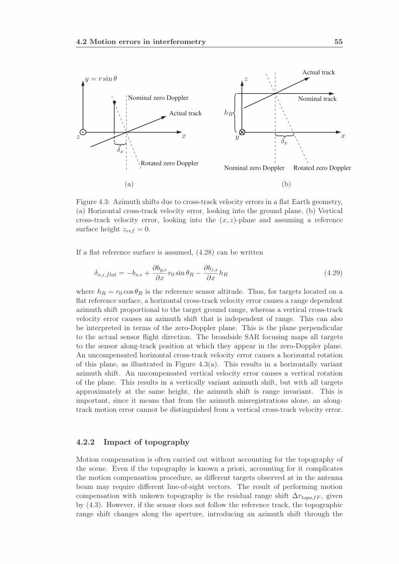
4.2 Motion errors in interferometry 55
Nominal zero Doppler
Rotated zero Doppler
Actual track
Nominal track
Actual track
Nominal zero Doppler Rotated zero Doppler
xx y
z
z
hR
(a) (b)
δxδx
y = r sin θ
Figure 4.3: Azimuth shifts due to cross-track velocity errors in a flat Earth geometry,(a) Horizontal cross-track velocity error, looking into the ground plane, (b) Verticalcross-track velocity error, looking into the (x, z)-plane and assuming a referencesurface height zref = 0.
If a flat reference surface is assumed, (4.28) can be written
δx,ǫ,flat = −bx,ǫ +∂by,ǫ∂x
r0 sin θR − ∂bz,ǫ∂x
hR (4.29)
where hR = r0 cos θR is the reference sensor altitude. Thus, for targets located on aflat reference surface, a horizontal cross-track velocity error causes a range dependentazimuth shift proportional to the target ground range, whereas a vertical cross-trackvelocity error causes an azimuth shift that is independent of range. This can alsobe interpreted in terms of the zero-Doppler plane. This is the plane perpendicularto the actual sensor flight direction. The broadside SAR focusing maps all targetsto the sensor along-track position at which they appear in the zero-Doppler plane.An uncompensated horizontal cross-track velocity error causes a horizontal rotationof this plane, as illustrated in Figure 4.3(a). This results in a horizontally variantazimuth shift. An uncompensated vertical velocity error causes a vertical rotationof the plane. This results in a vertically variant azimuth shift, but with all targetsapproximately at the same height, the azimuth shift is range invariant. This isimportant, since it means that from the azimuth misregistrations alone, an along-track motion error cannot be distinguished from a vertical cross-track velocity error.
4.2.2 Impact of topography
Motion compensation is often carried out without accounting for the topography ofthe scene. Even if the topography is known a priori, accounting for it complicatesthe motion compensation procedure, as different targets observed at in the antennabeam may require different line-of-sight vectors. The result of performing motioncompensation with unkown topography is the residual range shift ∆rtopo,IF , givenby (4.3). However, if the sensor does not follow the reference track, the topographicrange shift changes along the aperture, introducing an azimuth shift through the

56 Motion Errors in Repeat Track Interferometry
azimuth matched filter. Note that this shift is introduced by the motion compen-sation procedure and thus depends on the estimated sensor motion, not the motionestimation error. It occurs even in the absence of motion estimation errors.
Assuming that the estimated sensor motion can be considered linear within thesynthetic aperture of a single target, the same analysis as in section 4.2.1 can beapplied, interpreting the topographic range shift as a residual range shift on track2. From (4.23) it is seen that the linear along-track variation of the topographicshift does not affect the interferometric range shift. Thus the range shift due totopography is, as could be expected:
δr,topo = ∆rtopo,IF = − b⊥r0 sin θR
hT (4.30)
with ∆rtopo,IF given by (4.3). The azimuth shift due to uncompensated topographyis, from (4.27) and (4.3):
δx,topo = −r0∂∆rtopo,IF
∂x
=hT
sin θR
∂b⊥∂x
=1
sin θR
(∂by∂x
cos θR +∂bz∂x
sin θR
)hT
(4.31)
where hT is the target height over the reference surface to which motion compen-sation has been performed. Thus the azimuth shift is directly proportional to theperpendicular baseline velocity and to the height of the target above the referencesurface. There is no phase bias error associated with this shift, and thus it can beaccepted to the extent that it does not cause a loss of coherence, according to (4.12).
To give an idea of the magnitude of the topography-induced azimuth misregistrations,an example is in order. Assuming a 45◦ look angle, a sensor velocity of 240 m/s anda sensor cross-track velocity of 1 m/s perpendicular to the line-of-sight direction, atarget height of 100 m will lead to an azimuth shift of 0.6 m.
4.2.3 Summary of motion error model
The motion error model derived in section 4.2.1 assumes that the along-track vari-ation of the differential motion error can be considered linear within a syntheticaperture. For slowly varying motion errors caused by, for example, INU drift, this isa good approximation. For rapidly varying motion estimation errors which cannot beconsidered linear within an aperture, the model cannot be applied directly. In thatcase, only the slowly varying part of the motion may be estimated, leaving a residualmotion error along the aperture. If it is desired to estimate a rapidly varying motionerror, an option is to use a lower azimuth resolution, implying a shorter aperture. Ifthe motion error can be considered linear within the shorter aperture, the model canthen be applied.
The model for the topography-induced misregistrations in section 4.2.2 is based onthe assumption that the along-track variation of the estimated differential sensormotion can be considered linear within a synthetic aperture. In the absence ofmotion errors, the estimated sensor motion is also the actual sensor motion. In the

4.3 Estimating misregistration 57
EMISAR system, the flight control system causes a sinusoidal vertical motion of theaircraft with an amplitude of approximately 0.5 m and a period of typically 1 km to1.5 km. This period is comparable to the typical EMISAR synthetic aperture lengthat L-band, which is 800 m, assuming an azimuth resolution of 1.5 m and a rangeof 10 km. Thus, the actual sensor motion cannot necessarily be considered linearwithin an aperture, and this should be noted when applying the model (4.31).
When the sensor motion and the motion estimation errors can be considered linearwithin a synthetic aperture, the total observed range registration can, from sections4.2.1 and 4.2.2, be modeled by:
δr = δr,ǫ + δr,topo
≈ −b‖ǫ −b⊥
r0 sin θRhT
(4.32)
where b‖ǫ is the projection of the differential motion error onto the nominal line-of-sight direction (4.28) and b⊥ is the perpendicular baseline, given by (4.6). The lastterm of (4.32) is the interferometric range shift due to a target height, hT , above thereference surface. In topography mapping, this is the desired signal to be estimatedfrom the interferometric phase.
The total observed azimuth misregistration can be modeled by
δx = δx,ǫ + δx,topo
≈ −bx,ǫ + r0∂b‖ǫ
∂x+
hTsin θR
∂b⊥∂x
(4.33)
where bx,ǫ is the differential along-track motion error.
4.3 Estimating misregistration
The misregistration between two SAR images varies with both range and azimuthand can be estimated in several different ways. With traditional methods, the misreg-istrations are estimated at a number of evenly spaced image positions, and the shiftestimation is carried out by crosscorrelating patches around these positions. In thiswork, the spectral diversity method has been used, and this is briefly summarized inthe following.
4.3.1 Spectral Diversity Coregistration (SDC)
The Spectral Diversity Coregistration (SDC) algorithm [26] for estimating misregis-tration uses the fact that a displacement in the time (or spatial) domain is equivalentto a linear phase multiplication in the frequency domain. The basic principle is il-lustrated in Figure 4.4, and is the same whether the method is used for range orazimuth coregistration. The method was originally invented for absolute phase de-termination [27], where it is known as the split-spectrum algorithm. In the following,the principle of the algorithm is illustrated for estimating azimuth misregistration,but the method can equally well be applied in the range direction.
A point target located at the nominal position x = 0 is assumed. The impulseresponse in image 1 is displaced by ∆x1, and the impulse response in image 2 is

58 Motion Errors in Repeat Track Interferometry
0
Imag
e 1
Impulse response magnitude
0
Imag
e 2
Displacement
-0.5 0 0.5
Phase spectrum
0 0.5Normalized Frequency
-0.5 fA
fA
fB
fB
φT1 + φL1
2
φT1 − φL1
2
φT2 + φL2
2
φT2 − φL2
2
∆x1
∆x2
φA1
φB1
φA2
φB2
φT1
φT2
Figure 4.4: Illustration of Spectral Diversity Coregistration method.
displaced by ∆x2. The misregistration to be estimated is δx = ∆x2 − ∆x1. Goingto the frequency domain, the shifts are equivalent to linear phase factors. The linearphase in the frequency domain due to a shift in the time domain can be characterizedby the total variation of the phase, φL, over the bandwidth according to
φL = −2π∆x
ρx(4.34)
where ρx is the sample spacing in the x-direction.
The spectral diversity method starts by generating from each image, 1 and 2, twonon-overlapping low-resolution looks centered on the normalized frequencies fA andfB. The mean phase of the resulting low-resolution impulse responses is from Figure4.4
φA1 = φT1 + φL1fA φB1 = φT1 + φL1fB (4.35)
φA2 = φT2 + φL2fA φB2 = φT2 + φL2fB (4.36)
where the target phases, φT1 and φT2 contain contributions from topography, motionerrors and possibly other phase bias terms. Next, two low-resolution interferogramsare generated, one from the two low band looks, A, and one from the two high bandlooks, B. The phase of these interferograms is
φA = φA1 − φA2 = φT1 − φT2 + fA(φL1 − φL2) (4.37)
φB = φB1 − φB2 = φT1 − φT2 + fB(φL1 − φL2) (4.38)
Finally, a differential interferogram between the two low-resolution interferograms isformed to cancel the target phase terms
φSDC = φA − φB = (fA − fB)(φL1 − φL2) (4.39)

4.4 Estimating differential motion errors 59
Using (4.34), the shift can then be estimated by
δx = ∆x2 − ∆x1 =ρx
2π∆fφSDC (4.40)
where ∆f = fB − fA is the look center frequency separation relative to the full-resolution bandwidth.
Before using the spectral diversity method, the images should be registered to within±ρx/(2∆f) to avoid wrapping of the differential interferogram, and to get the maxi-mum coherence. For the example on Figure 4.4, fB− fA = 1
2 , and the images shouldthus be registered to within a resolution cell.
In [26] it is shown that the probability density function of the differential interfer-ogram phase is equal to the convolution of the probability density function of thetwo low-resolution interferograms, and therefore the differential phase is considerablymore noisy, leading to a noisy estimate of the image shifts. The estimate noise canbe reduced by averaging the differential interferograms. If N samples are averaged,it is shown in [28] that for N large, the variance of the spectral diversity shift estima-tor comes close to the theoretical minimum, which is achieved with a complex crosscorrelation. The spectral diversity algorithm, however is faster and simpler to im-plement, and insensitive to phase variations from the topography that are cancelledout in the differential interferogram formation. With the complex cross-correlationmethod, the topographic phase and other systematic phase contributions must beremoved prior to the correlation [28].
4.4 Estimating differential motion errors
The first step in differential motion error estimation is the estimation of δx andδr as a function of image coordinates. When patch-based methods such as speckletracking or coherence optimization are applied, the misregistration estimates aretypically only available at a subset of image positions. The SDC method describedin section 4.3.1 automatically provides estimates of the range misregistration for everysecond range sample, and estimates of the azimuth misregistration for every secondazimuth sample. Inverting the observed misregistrations to differential motion errorsis complicated by the fact that cross-track motion errors give rise to both rangeand azimuth misregistrations, whereas along-track errors give rise only to azimuthmisregistrations. There are generally two approaches to estimate the differentialmotion errors, parametric and non-parametric. These are described in the following.
4.4.1 Parametric motion error estimation
A method that uses image miregistrations for motion estimation is suggested in [29]and generalized in [30]. It is assumed that the baseline errors can be modeled by

60 Motion Errors in Repeat Track Interferometry
polynomia
bx,ǫ(x) =
px−1∑
k=0
bx,ǫ,kxk (4.41)
by,ǫ(x) =
py−1∑
k=0
by,ǫ,kxk (4.42)
bz,ǫ(x) =
pz−1∑
k=0
bz,ǫ,kxk (4.43)
Inserting these expressions into (4.32) and (4.33), and using several points in theimage, the coefficients of these polynomia can be obtained from a least squares fit,as described in [30].
With the parametric method, a polynomial fit to the baseline error is obtained inboth the along-track and each of the cross-track directions. The method is wellsuited for slowly varying errors (e.g. INU drifts) that can be modeled by polynomia.Furthermore, the method can be used when the motion errors are so large that shiftsof several resolution cells are seen and the images do not register at all. This could bethe case in systems where only non-kinematic GPS is available for correcting the INUmotion data. In principle, the method requires knowledge of the topography, sincethe range and azimuth misregistrations contains contributions from both motionerrors and topography. However, if the method is used over flat terrain, this can beneglected. Also, if the method is used as a preprocessing step to roughly registerthe images to within a resolution cell, the topography may also be ignored. This isespecially true in case of a small perpendicular baseline and moderate topography.
4.4.2 Non-parametric motion error estimation
A non-parametric method for differential motion error estimation is the algorithmproposed by Reigber in [2]. It is called the residual motion estimation algorithm, andwill in the following be referred to as the RME algorithm. The underlying assumptionis that the dominant contribution to the observed azimuth misregistration, δx, comesfrom the cross-track motion estimation error, δx,ǫ, and that azimuth misregistrationfrom along-track motion errors and unknown topography can be ignored (δx,topo ≈ 0and bx,ǫ ≈ 0) . With these assumptions, and the assumption that the motion errorcan be considered linear within an aperture, the observed azimuth misregistration ata given image coordinate is directly proportional to the projection of the derivativeof the motion error at that coordinate. Thus, the underlying assumption of the RMEalgorithm is that
δx ≈ r0∂b‖ǫ
∂x= r0(
∂by,ǫ∂x
sin θR − ∂bz,ǫ∂x
cos θR) (4.44)
Considering a single range bin at range r0, the differential motion error in this rangebin can be estimated to within a constant by:
b‖ǫ(x0, r0) =
∫ x0
0
δx(x, r0)
r0dx+ b‖ǫ,0(r0) (4.45)

4.4 Estimating differential motion errors 61
where b‖ǫ,0 is an unknown constant. With this approach, the differential motion erroris not limited to a polynomial variation. The spectral diversity method for estimatingmisregistration (see section 4.3.1) is convenient for this algorithm, since the outputestimates of the azimuth misregistrations are automatically closely spaced (two timesthe original azimuth pixel spacing), and no interpolation is necessary.
In the more general case, the variation of (4.44) across the range swath can be usedto estimate both the horizontal and the vertical components of the cross-track error.Consider a single along-track position, x0, where N estimates, δx1, δx2, . . . , δxN , ofthe azimuth misregistration are available, corresponding to the ranges r1, r2, . . . , rN .Then, from (4.44), a linear model can be set up:
χ = HP (4.46)
where the observation vector, χ is
χ =
δx1δx2...
δxN
(4.47)
and the sensitivity matrix, H , is
H =
r1 sin θR1 −r1 cos θR1
r2 sin θR2 −r2 cos θR2...
...rN sin θRN −rN cos θRN
(4.48)
The parameter vector is
P =
∂by,ǫ
∂x
∂bz,ǫ
∂x
(4.49)
The least squares solution to (4.46) provides an estimate of P :
P = H†χ (4.50)
where H† is the 2 ×N pseudo-inverse of H :
H† = (HTH)−1HT (4.51)
and
P =
∂bby,ǫ
∂x
∂bbz,ǫ
∂x
(4.52)
contains the estimated derivatives of the differential motion error. Using the spectraldiversity method, an estimate of the azimuth misregistration is available for everyrange position (N = NRA) but only for every second azimuth position, due to the twolooks. Solving (4.50) for every available range line, NAZ/2 estimates of (
∂by,ǫ
∂x,∂bz,ǫ
∂x)
62 Motion Errors in Repeat Track Interferometry
are available, and both estimates can then be integrated to obtain the differentialmotion error estimates to within a constant in each of the cross-track dimensions.
by,ǫ(x0) =
∫ x0
0
∂by,ǫ∂x
dx+ by,ǫ,0 (4.53)
bz,ǫ(x0) =
∫ x0
0
∂bz,ǫ∂x
dx+ bz,ǫ,0 (4.54)
where x0 is an arbitrary along track position, and by,ǫ,0, bz,ǫ,0 are unknown constants.
If the variation of the incidence angle across the swath is small, HTH becomesalmost singular, and the separation of the differential motion error derivatives intoa horizontal and vertical component becomes ill-conditioned. If the swath is nar-row enough to ignore the range variation of the motion-induced phase errors, theslant range projection of the differential motion error can be estimated as in (4.45),averaging over all ranges.
Even if the focused swath width is large enough to separate the baseline error intohorizontal and vertical components, misregistrations cannot be estimated for inco-herent areas in the images. To account for this, a coherence mask can be generated,indicating which pixels to exclude in the differential motion estimation. This exclu-sion is easily accomplished by removing rows of H, but if this reduces the swathwidth, the problem can again become ill-conditioned. An example of this is seen insection 6.3.3. Approaches for stabilizing the estimate in these situations should beexamined further, but it has not been done in this study.
If there are areas in the image where no valid misregistration estimates are availablefor a significant range of azimuth positions (e.g. a wide river flowing in the rangedirection across the image), the integrations (4.53) and (4.54) cannot be performedacross this area. In this case, the differential motion derivatives must be interpolatedacross this area. An approach for this has been suggested in [31]. This approachuses more than two subapertures in the spectral diversity misregistration estimation.This allows estimates of the misregistration to be obtained even over low-coherentareas, using that the azimuth impulse response from a high-coherent area can extendin to the low-coherent area. However, if the azimuth width of the low-coherent areais on the order of or larger than half the synthetic aperture width, this approach isalso not possible.
4.4.3 Estimating constant differential motion errors
As mentioned in section 4.2, a constant cross-track differential motion error (by,ǫ,0, bz,ǫ,0)does not give rise to azimuth shifts. This is also seen from (4.27), since for a constanterror, the derivatives of the error are 0. If the topography is unknown, it is generallyimpossible, whether using parametric or non-parametric motion error estimation, todistinguish whether the range shift caused by such an error is due to a motion error,or due to topography. In this case, the differential motion error must be estimatedusing an external digital elevation model or tie-points in the image.
A constant differential motion error will, from (4.25), result in a range shift
δr(r, x) = −by,ǫ,0 sin θT (r, x) + bz,ǫ,0 cos θT (r, x)
≈ −by,ǫ,0 sin θR(r) + bz,ǫ,0 cos θR(r)(4.55)
4.5 Correcting differential motion errors 63
The last approximation is valid for small motion errors and moderate topography,and allows estimates of the differential shift to be averaged over azimuth. Thus aconstant motion error will result in a range shift which is independent of along-trackposition but range dependent. This in turn results in an interferometric phase shift,according to (4.24). With the approach in [32], an external DEM is projected tothe image slant range geometry (see section 5.2.2) and a synthetic interferogramis generated, simulating the topographic phase contribution (4.4). The syntheticinterferogram is then subtracted from the unwrapped interferogram, and the phaseof this differential interferogram is, assuming that all time-varying motion errors havebeen corrected,
φs(r, x) = φabs + φǫ,0(r)
= φabs +4π
λ(−by,ǫ,0 sin θR(r) + bz,ǫ,0 cos θR(r))
= φabs −4π
λb‖ǫ,0(r)
(4.56)
which is independent of x. To reduce phase noise, φs can be averaged over the along-track dimension to obtain the range profile φs(r), from which the three unknownparameters, (φabs, by,ǫ,0, bz,ǫ,0) can be estimated. At each range, the range shift dueto the constant motion error is the projection of the constant motion error on thenominal line of sight direction at that range. A linear model can be set up
∆r1
...∆rN
=
1 − sin θ1 cos θ1...
......
1 − sin θN cos θN
λ4πφabsby,ǫ,0bz,ǫ,0
(4.57)
where ∆ri = λ4πφdiff (ri) are the samples of the φs(r) profile converted to a range
shift. The solution to (4.57) can be obtained the same way as in 4.4.2.
4.5 Correcting differential motion errors
When the differential motion errors have been estimated as described in 4.4.2, thereare several options to correct the SAR data, as illustrated in Figure 4.5.
(a) The simplest approach is to correct the interferogram phase using the estimatedbaseline errors. This does not correct the misregistration caused by the baselineerror, but if the errors are small enough that the misregistration does notsignificantly affect the coherence, this can be ignored. The correction thenbecomes a simple postprocessing step. Alternatively, the phase correction canbe supplemented by interpolation in the images before interferogram formation.The phase that is subtracted from the interferogram is given by (4.24).
(b) A method is suggested in [33] that, in addition to the phase error (4.24) alsocorrects the azimuth misregistration caused by the differential motion errors.This is achieved by inverting the azimuth compression of the slave image, ap-plying the phase correction, and recompressing. With fast FFT routines, thiscan be achieved more efficiently than phase correction and interpolation in

64 Motion Errors in Repeat Track Interferometry
Interferogram phase
Corrected IF phase
Image 2 SLC
FFT
FFT
Inverse Az. Compr.
IFFT
Az. Compr.
IFFT
Corrected Image 2
Image 2 Mocom Data
Refocus Image 2
Corrected Mocom Data
Raw Image 2 Data
Corrected Image 2
(a) (b) (c)
−4πλrǫ(r, x)
exp[j 4πλrǫ(r, x)
]
bǫ(x)
Figure 4.5: Correction of estimated differential motion errors, (a) Simple IF cor-rection, (b) Inverse azimuth compression approach, (c) Reprocessing with correctedmotion data.

4.5 Correcting differential motion errors 65
separate steps [34]. Alternatively, both master and slave can be corrected thisway, applying 50% of the correction to each image. In either case, the methoddoes not correct the range misregistration caused by the differential error, butthe range misregistration is typically much smaller than the corresponding az-imuth misregistrations. Since the correction is applied to image 2, the phasecorrection has the opposite sign as in (a).
(c) The most accurate way to correct the estimated baseline errors is to modifythe navigation data used for motion compensation and reprocess. This is moretime-consuming than the abovementioned methods, but also corrects the resid-ual range registration. Again, both images can be reprocessed with 50% of thebaseline correction or the slave image can be reprocessed with the entire cor-rection applied to the motion data for the slave image. When the correctionis applied to image 2, the estimated differential motion error, bǫ, is added tothe image 2 motion data. Note that with the RME algorithm described insection 4.4.2, only the cross-track components of the differential motion errorare estimated and corrected.


Chapter 5
Improved Non-parametric Motion
Error Estimation
As described in section 4.4, there are generally two ways to estimate differentialmotion errors in SAR interferometry, parametric and non-parametric. The non-parametric approach allows the estimation of motion errors that cannot be modeledby a polynomial, but it relies on the assumption that the observed azimuth misregis-trations do not contain contributions from along-track motion estimation errors, orfrom unknown topography.
In section 5.1, the influence of along-track errors on the non-parametric motion errorestimate is analyzed, and a method to distinguish along-track position errors fromcross-track velocity errors using an external DEM is proposed. This method relieson a parametric estimate of the along-track error, but the estimate of the cross-trackerror is still non-parametric.
The influence of topography on the non-parametric motion error estimate is difficultto quantify, as it depends on the actual topography and the tracks flown by thesensor. In section 5.2 a method to account for these errors using an external DEMis proposed.
The proposed schemes have been implemented in MATLAB and tested on EMISARdata. In section 5.3, the implementation is described, whereas the experimentalevaluation is presented in Chapter 6.
5.1 Along-track errors
A residual along track motion error, bx,ǫ(x), results directly in a corresponding az-imuth misregistration, see (4.27). If small, this error does not affect the image orinterferogram quality. However, if interpreted as a differential cross-track velocity er-ror by the RME algorithm, it leads to erroneous cross-track motion error estimates.This means that after correcting the SAR image(s) with the estimated motion error,a residual error occurs:
byz,ǫ = byz,ǫ − byz,ǫ (5.1)
where byz,ǫ is the actual cross-track motion error, byz,ǫ is the motion error estimatedby the RME algorithm and byz,ǫ is the residual error on the RME estimate, induced

68 Improved Non-parametric Motion Error Estimation
by along-track errors.
For the general case, where the differential motion error is resolved into both hor-izontal and vertical components, the impact of along-track errors can be analyzedby using (4.50). An along-track baseline error, bx,ǫ(x) causes an azimuth misregis-tration of δx = −bx,ǫ(x). For a single range line at azimuth positon x, the error onthe estimated derivatives of the differential cross-track error is then, from (5.1) and(4.46)
∂by,ǫ
∂x
∂bz,ǫ
∂x
= −H†
−bx,ǫ(x)−bx,ǫ(x)
...−bx,ǫ(x)
= H†
bx,ǫ(x)bx,ǫ(x)
...bx,ǫ(x)
(5.2)
where H† is the (2×N) pseudo-inverse of the sensitivity matrix (4.51). This can bewritten as
∂by,ǫ
∂x
∂bz,ǫ
∂x
=
[H†ybx,ǫ(x)
H†zbx,ǫ(x)
](5.3)
where
H†y =
N∑
i=1
H†1i (5.4)
H†z =
N∑
i=1
H†2i (5.5)
are the row sums of H† both in units of[m−1
].
In section 4.2.1 it was shown that in a flat Earth geometry, a horizontal velocityerror gives rise to a range-dependent azimuth shift, whereas a vertical velocity errorresults in an azimuth shift that is independent of range. An along-track motion erroralso results in a range-independent azimuth shift, so intuitively,
H†y,flat = 0 (5.6)
H†z,flat = − 1
hR(5.7)
where hR is the nominal sensor altiude above the reference terrain height used inmotion compensation and H†
z,flat is found from (4.29). Thus, a differential along-track motion error only affects the vertical baseline estimate. If the along-track erroris positive, then from (4.33), a negative azimuth shift occurs. From (4.29), a positivevelocity error also gives a negative azimuth shift, so a positive along-track error isestimated as a positive vertical velocity error. After correcting the motion data withthe RME motion error estimate, the residual error will then be a negative crosstrackvelocity, as indicated by (5.7).
For a non-flat Earth geometry, the values of H†y and H†
z can be evaluated. This hasbeen done for the EMISAR geometries used in Chapter 6. For the fl075 geometry(section 6.2), the sensor altitude over the reference surface is hR = 7504 m. For this

5.1 Along-track errors 69
geometry, H†y = −2.0×10⁻⁷ m−1 and H†
z = −1.3×10⁻⁴ m−1, so as expected |H†z | ≫
|H†y |. Furthermore, −1/H†
z = 7497 m ≈ hR. The same is seen for the fl045 geometry(section 6.3), where the altitude is hR = 12395 m In this case, H†
y = −2× 10⁻⁷ m−1
and H†z = −8.1 × 10⁻⁵ m−1. For this geometry also, −1/H†
z = 12378 m ≈ hR.
The residual error on the estimate of the differential motion error will be given by
by,ǫ(x) = H†y
∫ x
0bx,ǫ(x
′)dx′ ≈ 0 (5.8)
bz,ǫ(x) = H†z
∫ x
0bx,ǫ(x
′)dx′ ≈ − 1
hR
∫ x
0bx,ǫ(x
′)dx′ (5.9)
The validity of the approximation (5.8) can be evaluated for the fl045 scene, whichis approximately 100 km long. A constant bx,ǫ of 1 m will lead to a linearly growinghorizontal error, reaching a maximum at the edge of the image of by,ǫ(100 km) =−2.0 × 10⁻⁷ m−1 · 1 m · 100 km = −2 cm. The vertical error, bz,ǫ, will reach amaximum of −8.1 m. In this case the error from using the approximation (5.9) is1 cm.
For long strips, the vertical position error can grow significantly as an along-trackerror is integrated along the image. Linear and higher order along-track errors will in-troduce quadratic and higher-order cross-track errors, respectively. However, rapidlyvarying motion errors will not contribute significantly to the vertical error, sincethe integration in (5.9) suppresses rapidly varying errors. As an example, let thealong-track motion error be modeled as a sinusoid,
bx,ǫ = b0 cos 2πn
Lxx (5.10)
where b0 is the amplitude, n is the number of cycles of the error along the image andLx is the length of the image. The induced vertical error will, from (5.9) be:
bz,ǫ(x) =b0Lx
2πnhRsin 2π
n
Lxx (5.11)
which is inversely proportional to n.
If one or both images are corrected using the erroneous estimate of the vertical mo-tion error, bz,ǫ = bz,ǫ+ bz,ǫ, the induced cross-track error will compensate completelythe azimuth misregistration due to along-track errors, but cross-track errors are in-troduced instead. Since the impact of these are much more severe than a smalluncompensated azimuth misregistration, this must be accounted for.
5.1.1 Estimating along-track errors using External DEM
If an external DEM is available, the phase of the unwrapped, RME-corrected in-terferogram, φRME(x, r), can be compared to a synthetic interferogram, φsynt(x, r)generated from the external DEM and the motion data, as described in sections4.4.3 and 5.2.3. In the absence of other phase errors, this residual interferogramwill contain contributions from a constant phase offset, φabs, a constant differentialmotion error, bǫ,0, and the error induced by along track motion, bǫ. The residual

70 Improved Non-parametric Motion Error Estimation
interferogram phase, φRME,ǫ, is then, from (4.55) and (5.9)
φRME,ǫ(x, r) = φabs −4π
λ
(bǫ,0 + bǫ(x, r))
)· nT (x, r)
≈ φabs −4π
λ
(bǫ,0 + bǫ(x, r)
)· nR(r)
= φabs −4π
λ
(by,ǫ,0 sin θR(r) − bz,ǫ,0 cos θR(r) +
cos θR(r)
hR
∫ x
0bx,ǫ(x
′)dx′)
= φabs −4π
λ
(by,ǫ,0 sin θR(r) − bz,ǫ,0 cos θR(r) +
1
r
∫ x
0bx,ǫ(x
′)dx′)
(5.12)
An alternative to using the unwrapped interferogram is to use the range misregis-tration of image 1 and the corrected image 2, which is unambiguous, but a muchnoisier estimate of the shift (see section 4.3). The range misregistration may be use-ful in estimating the absolute phase offset, φabs, though. For moderate topography,if no DEM is available but a small perpendicular baseline is used, the expected to-pographic range shifts are small. In this case, the synthetic interferogram may notbe necessary at all, and the interferogram phase or range misregistration may beused on its own. However, if it is desired to estimate motion errors smaller than orcomparable to the topographic range shifts, an external DEM is necessary.
The along-track error is modeled as a p-order polynomial:
bx,ǫ(x) = bx,ǫ,0 + bx,ǫ,1x+ bx,ǫ,2x2 + · · · + bx,ǫ,px
p (5.13)
This is a reasonable approximation, since, as indicated in the previous section, rapidvariations in the along-track error will not significantly affect the RME estimate,due to the integration. For small along-track errors, it is not necessary to know theactual along-track error, only the part that affects the cross-track motion estimatesignificantly. The integral in (5.9) becomes:
∫ x
0bx,ǫ(x
′)dx′ = bx,ǫ,0x+1
2bx,ǫ,1x
2 +1
3bx,ǫ,2x
3 + · · · + 1
p+ 1bx,ǫ,px
p+1 (5.14)
Taking well-distributed samples across the residual phase interferogram at points(ri, xj) where i = 1 . . . N and j = 1 . . .M , and converting the residual phase, φRME,ǫ,to residual range shifts, ∆rij , a linear model can be set up
ρ = KQ (5.15)
where the observation vector is now N ·M×1 and contains the samples of the residualinterferogram (converted from phase to range shift):
ρ =
∆r11...
∆rij...
∆rNM
=
λ
4π
φRME,ǫ(r1, x1)...
φRME,ǫ(ri, xj)...
φRME,ǫ(rN , xM )
(5.16)

5.1 Along-track errors 71
The sensitivity matrix is N ·M × (p+ 4)
K =
1 − sin θ1 cos θ1 − 1r1x1 − 1
2r1x2
1 . . . − 1(p+1)r1
xp+11
......
......
.... . .
...1 − sin θi cos θi − 1
rixj − 1
2rix2j . . . − 1
(p+1)rixp+1j
......
......
.... . .
...1 − sin θN cos θN − 1
rNxM − 1
2rNx2M . . . − 1
(p+1)rNxp+1M
(5.17)
The parameter vector is
Q =
∆rabsby,ǫ,0bz,ǫ,0bx,ǫ,0bx,ǫ,1
...bx,ǫ,p
(5.18)
Instead of estimating directly the polynomial coefficients of bx it is advantageous toreformulate (5.13) using Chebyshev polynomials:
bx(x) = βx0T0(x) + βx1T1(x) + βx2T2(x) + · · · + βxpTp(x) (5.19)
where Ti(x) are the i-order Chebyshev polynomials of the first kind and x is
x =x− 1
2(xM + x0)12(xM − x0)
(5.20)
Since the Chebyshev polynomials are orthogonal and normalized, the magnitude ofthe estimated coefficients can be interpreted directly as the magnitude of each of theterms of (5.19).
When (5.15) has been solved to obtain the estimate, Q, of (5.18), the along-trackmotion error estimate, bx,ǫ can be calculated from (5.19). The estimate of the residualvertical motion error induced by along-track motion can be obtained from:
bz,ǫ(x) = − 1
hR
∫ x
0bx,ǫ(x
′)dx′ (5.21)
where the integral can be calculated from the estimated along-track motion errorcoefficients and (5.19). The estimated constant differential motion error components,(by,ǫ,0, bz,ǫ,0) should also be added to the cross-track motion error estimate.
When the corrections calculated by the along-track motion estimation are small anddo not cause appreciable misregistration, it is sufficient to phase correct the interfero-gram by the estimated cross-track errors, as described in section 4.5. If the navigationdata are corrected, the along-track coordinate should also be corrected, otherwise theestimated along-track error will be converted to azimuth misregistration.

72 Improved Non-parametric Motion Error Estimation
5.1.2 Summary of algorithm
The final along-track correction scheme is summarized here:
1. Perform standard non-parametric RME estimation (section 4.4.2) and correc-tion (section 4.5), ignoring along-track errors.
2. Generate interferogram from RME-corrected data and subtract the syntheticinterferogram to obtain a residual interferogram, φRME,ǫ.
3. Take samples of the residual interferogram to obtain the observation vector, ρ
(eq. 5.16).
4. Calculate the sensitivity matrix, K (eq. (5.17)) using a p-order model for theresidual along-track error.
5. Solve for Q (eq. (5.18)) using the standard least squares solution (4.50).
6. Calculate the final vertical motion correction from (5.21). This is a p+1-ordercorrection, due to the integral.
7. Correct final motion error (see section 4.5) by interferogram phase correctionor complete refocusing using corrected navigation data (including the p-orderalong-track correction). The inverse azimuth compression scheme cannot beused, as it cannot correct a non-constant along-track error without modifyingthe phase of the refocused image.
The proposed method is, like the basic RME algorithm, capable of correcting ar-bitrary cross-track motion errors, as this is done in the initial RME estimation.Since the cross-track errors induced by along-track residual motion will be of a low-frequency nature, due to the integration, it is reasonable to assume that the majorcontribution can be modeled by a polynomial. If the obtained estimate does notmodel the observed residual phase error, the order, p, of the along-track motionmodel can be increased. The method has been tested on EMISAR images as de-scribed in sections 6.2.4 and 6.3.4.
5.2 Impact of topography
5.2.1 Accounting for spherical Earth geometry
To accurately apply an external digital elevation model in SAR processing, it isnecessary to account for the spherical Earth geometry. As mentioned in section5.3, the sarif range-Doppler SAR processor [21] has been used in this project.This processor uses the (s, c, h)-coordinate system [29]. The (s, c, h)-coordinates arecurvilinear coordinates on a reference sphere that locally approximates the WGS-84Earth model ellipsoid [10]. It is defined by first selecting the approximate midpointof the reference track as the origin of the (s, c, h)-system. The approximating sphereis selected so that it is tangent to the ellipsoid at the origin and has the same radiusof curvature as the ellipsoid in the reference track direction. Then s is the along-trackcoordinate, c the cross-track coordinate and h the altitude over the reference sphere.The reference track is then defined by pR(s) = (s, cR, hR) where cR, hR are constants

5.2 Impact of topography 73
for the given reference track. The s and c coordinates are actually arc lengths onthe reference sphere, but for the aircraft geometry they can be considered locallycartesian (i.e. within an aperture, and when evaluating the effects of for examplemotion compensation).
5.2.2 External DEM projection to slant range geometry
To use an external DEM, this must first be converted to the SAR image slant rangegeometry. In this work, the external DEM used is the Shuttle Radar TopographyMission 3 arcminute (SRTM-3) DEM [35]. This is supplied as a 3-arcminute (≈90 m) grid of latitude, longitude and geoid height values. First, a subset of theDEM covering the imaged area is extracted. Then the geoid heights are convertedto ellipsoid heights using a geoid model, and the coordinates are converted from(latitude, longitude, ellipsoid height) to the reference (s, c, h) system used in theprocessing. In [29], the following relations between target coordinates, slant range,and reference track coordinates are given:
sT = sR + rnsRa
Ra + hT(5.22)
cT = cR + rncRa
Ra + hT(5.23)
hT = hR + rnh +r2(n2s + n2
c
)
2 (Ra + hR + rnh)(5.24)
where (sT , cT , hT ) are the coordinates of the DEM point, (sR, cR, hR) are the refer-ence track coordinates, r is the distance from the reference track to the DEM point,nT = (ns, nc, nh) is the line-of-sight vector from the reference track to the target,and Ra is the radius of the approximating sphere. For a broadside looking SAR,ns = 0, so sR = sT . Note that the definition of hR used here is slightly differentfrom the one used in sections 5.1 and 4.2.1, where it defines the sensor altitude overthe reference surface used in motion compensation. The reference surface might notbe located on the reference ellipsoid but at some constant offset altitude, href .
With little error, the denominator of (5.24) can be approximated by 2Ra, sincehR ≈ −rnh. From (5.23) and (5.24), and using that n2
c + n2h = 1, three equations
can be set up
rnc =(cT − cR)(Ra+ hT )
Ra(5.25)
rnh = hT − hR − r2n2c
2Ra(5.26)
r =√r2n2
c + r2n2h (5.27)
from which r can readily be obtained. Applying this procedure to each DEM pointresults in a nonuniform grid of (s, r, h)-points, and a twodimensional resamplingcan be used to obtain a rectangular grid with the desired spacing in the imagerange and azimuth coordinates. This can be done under the assumption of moderatetopography with no severe layover. The principle is illustrated in Figure 5.1

74 Improved Non-parametric Motion Error Estimation
sss
c rr
Lat
Lon
(a) (b) (c) (d)
Figure 5.1: External DEM projection. (a) External DEM, (b) Converted to (s, c, h),(c) Converted to (s, r, h), (d) Resampled to uniform (s, r) grid.
5.2.3 Generation of synthetic interferogram
A synthetic interferogram can be generated concurrently with the DEM projectiondescribed in the previous section. For each DEM point that has been converted to thereference (s, c, h) geometry, the range to the master and slave track positions can becalculated, and the difference formed. This range difference can again be resampledto a rectangular grid in the image coordinates. If the dual reference track approachis used, the synthetic interferogram should be generated using the nominal masterand slave tracks. For the common reference track approach, which has been used inthis work, the actual sensor positions should be used. The motion data must in thiscase be interpolated at the along-track positions, sT , at which the DEM points areavailable. Following the resampling to image coordinates, the phase shifts that havebeen applied in the motion compensation are applied to the synthetic interferogram.
5.2.4 Modeling azimuth misregistration from topography
According to (4.31), targets at an elevation different from the reference elevationused in motion compensation will cause an azimuth misregistration proportional tothe cross-track velocities with which the data were acquired. If the azimuth mis-registration is used in differential motion error estimation, the topography-inducedmisregistration will be interpreted wrongly as due to cross-track velocities, see sec-tion 4.4. It is therefore important that the cross-track velocities are minimized, butthis depends on the flight control system used in the SAR aircraft platform. Forexample, the flight control system used for EMISAR on the Gulfstream G3 suffersfrom servo loop oscillations, leading to typical vertical cross-track velocities of upto 0.5 m/s. It is difficult to qualitatively assess the impact of topography on theresidual motion estimate, but it can be exemplified using actual navigation data anda DEM. A simple method for modeling the misregistration from topography usingan external DEM and navigation data is presented in the following. The methoduses the fact that the topography-induced azimuth misregistration is caused by themotion compensation – which is known – coupling with the topography, which canbe supplied from the external DEM.
For each output range line in the image, the vertical and horizontal cross-track ve-locities for each track can be obtained from the navigation data. Then, the expected
5.3 Implementation 75
azimuth misregistration in each range bin can be calculated using (4.31):
δx,topo(s; r) =hT (s, r)
sin θR(r)
∂b⊥∂s
(s, r)
=hT (s, r)
sin θR(r)
((∂c2(s)
∂s− ∂c1(s)
∂s) cos θR(r) + (
∂h2(s)
∂s− ∂h1(s)
∂s) sin θR(r)
)
(5.28)
where s has now been used as the along-track coordinate, (c1(s), c2(s), h1(s), h2(s)) isthe cross-track motion estimate from the navigation data, and hT is the target terrainheight supplied from the external DEM. The estimate is smoothed by applying arectangular filter, with the filter length set equal to the synthetic aperture length forthe given azimuth line. Calculating (5.28) for each range bin results in a syntheticazimuth misregistration image. The topographic misregistration can be subtractedfrom the azimuth misregistration obtained by, for example, the spectral diversityalgorithm. The corrected misregistrations can then be used as input to a differentialmotion estimation algorithm. Thus, the azimuth shifts input to, for example, theRME algorithm (section 4.4.2) can be written:
δx,RME = δx,SDC − δx,topo (5.29)
where δx,SDC is the azimuth misregistration estimate obtained by the spectral diver-sity algorithm.
The method described above can be used to subtract the topography-induced mis-registration before RME estimaton. This way, the RME estimate can be improved,and it also gives an idea of the errors that can be expected if an external DEM isnot available. The method does not, however, correct the topography-induced mis-registrations. Thus, it is applicable when the topography induced misregistrationsare small enough that the coherence is not severely affected (see (4.12)), but largeenough that the baseline estimate may be affected.
In the event that the influence of the topography-induced azimuth misregistrationson the coherence cannot be neglected, topography-dependent motion compensationmust be applied, but this complicates the processing considerably, and has not beenexamined in this work. A method for topographic motion compensation that hasbeen applied in conjunction with the RME algorithm is given in [36].
5.3 Implementation
MATLAB programs were designed to read the output files setup and radar data filesfrom the sarif SAR processor, developed by Johan Mohr, which has been used in thiswork. A tiled image format and input/output routines for MATLAB were developedto allow easy range and azimuth access to large image files. Then, the methods fornon-parametric motion estimation were implemented, including the improvementsdescribed in this chapter. A block diagram of the implemented routines is shown onFigure 5.2.

76 Improved Non-parametric Motion Error Estimation
Image 1 SLC
Output from sarif*
Image 2 SLC
Navigation Data
SRTM DEM
SDC Misreg Estimate
spec_div_rat_rbw
RME Estimation w/Topo Correct.
est_baseline_error
Along-track error estimation
est_along_cheby
Correct Image 2
invert_azc
Correct Interferogram Phase
IF_correct
Project DEM to slant range
generate_dem
Generate Synthetic IF
synti
Interferogram Formation
inftml*
Calculate Topo. Az. Misreg
topo_az_misreg
Final Corrected IF
Phase Unwrapping
miniuw*
Int.
Figure 5.2: MATLAB implementation of non-parametric motion estimation with theimprovements described in Chapter 5. An asterisk indicates an external program notdeveloped by the author. Note that the estimation of a constant cross-track baselineerror and an absolute phase offset is included in est_along_cheby.

5.3 Implementation 77
0 5000 10000 150000
1000
2000
3000
4000EMIDIF misregistration estimate [m]
Azimuth [samples]
Ran
ge [s
ampl
es]
−0.6
−0.4
−0.2
0
0.2
0.4
0.6
0 5000 10000 150000
1000
2000
3000
4000SDC misregistration estimate [m]
Ran
ge [s
ampl
es]
Azimuth [samples]
−0.6
−0.4
−0.2
0
0.2
0.4
0.6
Figure 5.3: Comparison of SDC and emidif algorithms for azimuth misregistratonestimation.
5.3.1 Implementation of SDC and RME algorithms
The Spectral Diversity algorithm, described in section 4.3.1, was implemented inMATLAB, to be used on focused EMISAR data. For verification, the spectral di-versity algorithm was compared to the emidif speckle correlation algorithm for mis-registration estimation using the two SAR images in Section 6.2. Only azimuthmisregistrations were considered. The filter applied to the SDC estimate was a rect-angular filter of the same dimensions as the patch size used in emidif, and the SDCestimates were extracted at the 2667 positions at which valid emidif estimates wereavailable. The two misregistration images are shown in Figure 5.3. It is seen that theimages resemble each other, but the emidif estimates are considerably more noisy.The mean difference of the emidif and SDC estimates is 0.9 mm whereas the RMSvalue of the differences is 16 cm. This is probably caused by the noise on the emidif
estimates.
The RME algorithm, as described in section 4.4.2, was also implemented in MAT-LAB. This takes as input an azimuth misregistration image, a coherence mask, and

78 Improved Non-parametric Motion Error Estimation
navigation data output by sarif. The coherence mask is used to exclude decorre-lated areas from the RME estimation. Note that the coherence mask is not shownon the block diagram.
A verification of the implemented SDC and RME processing was carried out by pro-cessing the L-band data used in section 6.2 and performing the RME estimation.Then the motion data for one image were artificially modified with a slow sinusoidalvariation (one half period along the 25 km image) in the horizontal cross-track coor-dinate. The vertical motion data were modified by the sum of a slow and a fast (sixperiods along the image) sinusoidal error. All sinusoids had a peak-to-peak variationof 6 cm. The image was refocused, and a new SDC misregistration estimation andRME estimation was carried out. Ideally, the difference between the estimated resid-ual motion errors should be equal to the artificial errors. In practice, the deviationfrom the artificial error was less than 2 mm, with no systematic variation except forthe constant baseline error, which cannot be detected by the RME algorithm.
5.3.2 Implementation of improved RME
The DEM projection (section 5.2.2) was implemented in MATLAB based upon ex-isting FORTRAN routines for conversion between (Lat,Lon,Alt) and (s, c, h) coor-dinate systems. These were vectorized and converted to MATLAB, and a routinefor reading SRTM DEM data was written. This could be modified to other typesof elevation data also. The resampling of the slant range projected DEM to imagecoordinates was accomplished with the MATLAB griddata routine, which performsbicubic interpolation on unevenly spaced data.
The synthetic interferogram generation (section 5.2.3) and topographic compensa-tion (section 5.2.4) were implemented in MATLAB. The topographic compensationroutine generates a synthetic misregistration image from the navigation data andthe DEM data, and this synthetic image is subtracted from the SDC misregistrationimage prior to RME estimation.
Finally, the along-track motion estimation proposed in section 5.1.1 was implementedin MATLAB, including the modification to use Chebyshev polynomials. Note thatthis along-track error estimation also estimates a constant cross-track baseline offset,which must be estimated from the topography. MATLAB is well suited for least-squares solution of large systems like (5.15).

Chapter 6
Experimental Evaluation
The RME algorithm (section 4.4) and its suggested improvements (chapter 5) havebeen implemented in MATLAB and tested on EMISAR data. Two different zero-Doppler RTI data sets have been used, both with a temporal baseline of less thanan hour. The first is HH-polarisation L-band (λ = 24 cm) data set (Flight fl075
maps m1314 and m1352) acquired in June 1999 over Foulum in Jutland, a mainlyagricultural scene. Kinematic GPS data are available here, and the baseline used issensitive to topography. The strip length is 4096× 15000 samples (range×azimuth),or 6.14 km× 22.5 km, with the nominal 1.5 m resolution in both dimensions. Thedata were obtained from an altitude of 25000 feet, with a near range incidence angleof 37.4◦.
The second data set (Flight fl045 maps m0757 and m0841) is a HH-polarisationC-band set (λ = 5.66 cm), and acquired in July 1996. Here the focused strip is6144×65536 samples, or 9.2 km×98.3 km, extending from Foulum out into Kattegat.The data were obtained from an altitude of 41,000 feet, with a near range incidenceangle of 36.7◦. Only the Gulfstream G3 GPS and EMISAR INU (not EGI) navigationdata are available for this scene. The areas covered by the two data sets are illustratedin Figure 6.1. The topography variations over the scenes are on the order of 100 m,as can be seen from the topographic maps in Figures 6.4 and 6.16.
6.1 Data processing
The data processing carried out in this chapter is illustrated in Figure 6.2. The SARimages were initially focused to 1.5 m range and azimuth resolution using the sarif
range-Doppler processor and associated tool chain, developed by Johan Mohr [21].Before the initial focusing, the INU navigation data were corrected by a third-orderpolynomial fit of each of the (s, c, h) coordinates to the GPS data to correct for INUdrift. The data were focused to common reference tracks (i.e. one reference trackfor each dataset). For the C-band data this is natural, since the actual baseline wassmall (less than 10 m). For the L-band data, it could be considered to use separatereference tracks, due to the relatively large baseline, but for simplicity, a commonreference track was also used here.
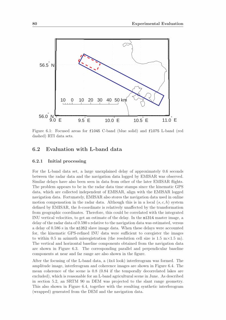
80 Experimental Evaluation
0 10 20 30 40 50 km10
9.0˚ E 9.5˚ E 10.0˚ E 10.5˚ E 11.0˚ E 56.0˚ N
56.5˚ N
Figure 6.1: Focused areas for fl045 C-band (blue solid) and fl075 L-band (reddashed) RTI data sets.
6.2 Evaluation with L-band data
6.2.1 Initial processing
For the L-band data set, a large unexplained delay of approximately 0.6 secondsbetween the radar data and the navigation data logged by EMISAR was observed.Similar delays have also been seen in data from other of the later EMISAR flights.The problem appears to be in the radar data time stamps since the kinematic GPSdata, which are collected independent of EMISAR, align with the EMISAR loggednavigation data. Fortunately, EMISAR also stores the navigation data used in onlinemotion compensation in the radar data. Although this is in a local (s, c, h) systemdefined by EMISAR, the h-coordinate is relatively unaffected by the transformationfrom geographic coordinates. Therefore, this could be correlated with the integratedINU vertical velocities, to get an estimate of the delay. In the m1314 master image, adelay of the radar data of 0.590 s relative to the navigation data was estimated, versusa delay of 0.586 s in the m1352 slave image data. When these delays were accountedfor, the kinematic GPS-refined INU data were sufficient to coregister the imagesto within 0.5 m azimuth misregistration (the resolution cell size is 1.5 m×1.5 m).The vertical and horizontal baseline components obtained from the navigation dataare shown in Figure 6.3. The corresponding parallel and perpendicular baselinecomponents at near and far range are also shown in the figure.
After the focusing of the L-band data, a (4x4 look) interferogram was formed. Theamplitude image, interferogram and coherence images are shown in Figure 6.4. Themean coherence of the scene is 0.8 (0.84 if the temporally decorrelated lakes areexcluded), which is reasonable for an L-band agricultural scene in June. As describedin section 5.2, an SRTM 90 m DEM was projected to the slant range geometry.This also shown in Figure 6.4, together with the resulting synthetic interferogram(wrapped) generated from the DEM and the navigation data.

6.2 Evaluation with L-band data 81
Figure 6.2: Processing flow.

82 Experimental Evaluation
0 5 10 15 20 25
30
25
20
Azimuth [km]
[m]
Baseline
yz
0 5 10 15 20 25−20
−10
0
10Parallel baseline variation
Azimuth [km]
Par
. bas
elin
e [m
] Near rangeFar range
0 5 10 15 20 25−45
−40
−35
−30
−25Perpendicular baseline variation
Azimuth [km]
Per
. bas
elin
e [m
] Near rangeFar range
Figure 6.3: Baseline components for the fl075 L-band data, from navigation data.

6.2 Evaluation with L-band data 83
Azimuth [km]
Ran
ge [k
m]
0 5 10 15 200
2
4
6
Azimuth [km]
Ran
ge [k
m]
0 5 10 15 200
2
4
6
0
π
−π
Azimuth [km]
Ran
ge [k
m]
0 5 10 15 200
2
4
6
0
0.5
1
Azimuth [km]
Ran
ge [k
m]
0 5 10 15 200
2
4
6
−60
−40
−20
0
Azimuth [km]
Ran
ge [k
m]
0 5 10 15 200
2
4
6
0
π
−π
Figure 6.4: fl075 data after initial focusing and 4x4 multilook, from top down: Am-plitude, interferometric phase, coherence, DEM (relative to mocom height), syntheticinterferogram from external DEM.

84 Experimental Evaluation
6.2.2 SDC processing
The range and azimuth misregistrations were estimated by the spectral diversity al-gorithm as described in section 4.3.1. The algorithms developed in principle do notrely on the range misregistration, but it is shown for reference. In both cases, theSDC complex differential interferogram was normalized and filtered using a 201×201Gaussian kernel before being converted to displacement estimates. The filtering re-duces the estimation noise, as well as the impact of small decorrelated areas. Figure6.5 shows the azimuth misregistration image estimated this way. The major varia-
Azimuth [km]
Ran
ge [k
m]
Azimuth Misreg [m]
0 5 10 15 200
2
4
6
−0.5
0
0.5
Azimuth [km]
Ran
ge [k
m]
Azimuth Misreg minus Topography Contribution [m]
0 5 10 15 200
2
4
6
−0.5
0
0.5
Azimuth [km]
Ran
ge [k
m]
Simulated Topographic Az. Misreg [m]
0 5 10 15 200
2
4
6
−0.5
0
0.5
Figure 6.5: Azimuth spectral diversity misregistration estimates for fl075, with andwithout simulated topography-induced azimuth misregistration.
tion of the azimuth misregistration is seen in the azimuth direction. There is alsosome variation in range, though, indicating that at least part of the misregistrationis induced by horizontal cross-track errors. The misregistrations vary rapidly, whichsuggests that they are caused by an uncompensated delay between radar and navi-gation data in one or both images. This suspicion is strengthened by the fact thata mean misregistration of -9.6 cm is seen. Of course this could be due to a constant

6.2 Evaluation with L-band data 85
along-track motion errror, but it could also be caused by an uncompensated delay of9.6 cm/(240 m/s) = 0.0004 s, and it is likely that the observed 0.6 s radar timestampdelays cannot be estimated completely by the approach mentioned in Section 6.1.The mean misregistration could also be due to a constant vertical velocity error of−9.6 cm/7620 m ≈ 1.3 × 10⁻⁵ m/m, according to (5.9). This would lead to a linearvariation of the vertical error of 0.32 m along the image, which should be visiblein the range registration, but this is not the case (see Figure 6.6). It is possibleto estimate the delay between radar data and navigation data in each image fromthe observed azimuth misregistrations [21]. This was attempted, but without succes.Anyway, the effect of such delays are basically differential motion errors (in bothalong- and cross-track directions), and it provides an opportunity to test the residualmotion estimation methods described in this work. This is an area that should beanalysed further, though.
Figure 6.5 also shows the simulated azimuth misregistration from topography, ob-tained by the method described in 5.2.4, and the azimuth misregistration image aftersubtraction of the simulated topography contribution. The topographic correctionseems to remove some of the cloudiness of the original misregistration image, but theeffect is minor, and nothing conclusive can be said from this.
The estimated range misregistration is shown in Figure 6.6, together with the rangemisregistration simulated from the external DEM and the navigation data. Also, thedifference between the estimated and the simulated range registration is shown. Theexpected variations from the evaluation of the external DEM and the navigationdata are on the order of 0.5 m, and this is also seen in the range misregistrationimage. The difference between the two images is most likely due to the differentialcross-track errors.
6.2.3 RME estimation and correction
The basic RME algorithm was applied to the azimuth misregistration image to obtainestimates of the residual cross-track motion, as described in 4.4.2. As the meanmisregistration is likely due to along-track errors, caused either by an uncompensateddelay between radar and navigation data or a constant along-track error (see previoussection), it was subtracted before the RME estimation. This is not strictly necessarywith the along-track error estimation described in section 5.1.1, and in fact this wastested, as described in 6.2.4.
The estimated motion errors are shown on Figure 6.7, both for the case when the sim-ulated topography was subtracted before RME estimation, and for the case where itwas not. It can be seen that in both cases, the estimated errors have the same shape,with a larger variation in the vertical than in the horizontal cross-track component.Without topographic compensation, the total variation in the vertical component is10 cm, whereas it is 7 cm with topographic compensation. Since the accuracy ofkinematic GPS is generally considered to be 5-10 cm this is not unreasonable. Thedifference in the estimates with and without topography is within 5 cm. This is alarge variation compared to the actual estimated errors, but it cannot be concludedfrom this which estimate is correct.
Since the estimated cross-track errors are small compared to the overall topographicinterferometric shifts of up to 0.5 m, it is sufficient to correct the slave image using

86 Experimental Evaluation
Ran
ge [k
m]
Range Misreg [m]
0 5 10 15 200
1
2
3
4
5
6
−0.5
−0.4
−0.3
−0.2
−0.1
0
0.1
Ran
ge [k
m]
Simulated Range Misreg from Topography [m]
0 5 10 15 200
1
2
3
4
5
6
−0.5
−0.4
−0.3
−0.2
−0.1
0
0.1
Ran
ge [k
m]
Azimuth [km]
Actual Range Misreg minus Simulated Misreg [m]
0 5 10 15 200
1
2
3
4
5
6
−0.2
−0.15
−0.1
−0.05
0
z/Up
Figure 6.6: (top) Range spectral diversity misregistration estimates for fl075 data,(middle) Simulated range misregistration from external DEM and navigation data(middle), (bottom) Difference of estimated and simulated misregistrations.

6.2 Evaluation with L-band data 87
0 5 10 15 20 25−0.12
−0.1
−0.08
−0.06
−0.04
−0.02
0
0.02
[m]
No topography compensation
0 5 10 15 20 25−0.12
−0.1
−0.08
−0.06
−0.04
−0.02
0
0.02
[m]
With topography compensation
0 5 10 15 20 25−0.05
0
0.05
Azimuth [km]
[m]
Difference in estimates
by,ǫ
by,ǫ
by,ǫ
bz,ǫ
bz,ǫ
bz,ǫ
Figure 6.7: fl075 Cross-track residual errors estimated by basic RME algorithm,(top) Without topography compensation, (middle) With topography compensation,(bottom) Difference in estimates.

88 Experimental Evaluation
only azimuth refocusing (see section 4.5) as this corrects the phase shift and az-imuth misregistrations from the residual cross-track motion. This was done for bothcases (with and without topographic compensation). The spectral diversity mis-registration estimate for the images that were RME corrected without topographycompensation is shown on Figure 6.8. The residual misregistration for the imagesthat were corrected with topography compensation is shown on Figure 6.9. Alsoshown is the simulated residual misregistration due to topography. This is the part ofthe simulated topographic azimuth misregistration that is not modeled by the RMEestimation. For the images corrected with topography compensation, the expectedresidual azimuth misregistration is simply the estimated topographic misregistra-tion which was subtracted before RME correction. In the case where topographiccompensation is not applied prior to RME, part of the topographic misregistrationis interpreted as due to across-track errors. The simulated residual misregistrationwas found by using the RME correction on the synthetic topographic misregistrationimage. The figure also shows the difference between the actual and the simulatedmisregistrations, which should ideally be zero. In both cases, the simulated resid-ual misregistration resembles the actual misregistration. The difference between theestimated and simulated residual misregistration shows non-systematic variations of±10 cm, but there seems to be a slight correlation between the difference image andthe simulated topographic misregistration, suggesting that the topographic misreg-istration is slightly undercompensated. This could be caused by the lower resolutionof the SRTM DEM compared to the image resolution. It could also be caused bythe fact that a rectangular filter of length equal to the aperture length is used inthe topographic misregistration estimation (see section 5.2.4) but the azimuth com-pression uses a weighted compression filter to suppress sidelobes, implying a shortereffective aperture. The EMISAR flight control system causes a vertical oscillation ofthe flown track with a period of approximately 1250 m. This gives rise to azimuthmisregistrations, but the synthetic aperture length at midswath is approximately800 m, so the motion cannot be considered linear within the aperture. The longerthe effective aperture, the more the oscillating motion will be averaged out, implyingsmaller azimuth shifts, and this might explain the residual misregistrations. It wasattempted to adjust the filter length used in the topographic compensation to bet-ter match the effective aperture length, but the results were inconclusive. Actuallyit was found that when the filter became too short, the topographic compensationovercompensated the misregistration images, so this is a subject worthy of furtherstudy.
The coherence histograms before and after the RME correction are shown on figure6.10. The coherence is generally high to begin with, but a slight improvement isseen for the corrected images. There is no distinguishable difference between thecoherence histograms with regards to topography misregistration compensation. Thisis not surprising, as the topography misregistration effect is small compared to thecross-track induced azimuth misregistrations (see figure 6.5).
6.2.4 Along-track motion estimation
The RME corrected interferograms were Goldstein-filtered and unwrapped using aMinimum Cost-unwrapper, miniUW. Then the synthetic interferogram (see Figures6.4 and 6.6 for the wrapped and unwrapped synthetic interferogram, respectively)

6.2 Evaluation with L-band data 89
Ran
ge [k
m]
Residual azimuth misreg, no topocomp [m]
0 5 10 15 200
1
2
3
4
5
6
−0.5
0
0.5
Simulated residual misreg, no topocomp [m]
Ran
ge [k
m]
0 5 10 15 200
1
2
3
4
5
6
−0.5
0
0.5
Residual minus simulated Misreg, no topocomp [m]
Ran
ge [k
m]
Azimuth [km]0 5 10 15 20
0
1
2
3
4
5
6
−0.1
−0.05
0
0.05
0.1
Figure 6.8: Residual azimuth misregistration after RME correction without topo-graphic correction,(top) Estimated residual misregistration (middle) Simulated resid-ual misregistration due to topography, (bottom) Difference between estimated andsimulated residual misregistration.

90 Experimental Evaluation
Ran
ge [k
m]
Residual azimuth misreg, w/ topocomp [m]
0 5 10 15 200
1
2
3
4
5
6
−0.5
0
0.5
Simulated residual misreg, w/ topocomp [m]
Ran
ge [k
m]
0 5 10 15 200
1
2
3
4
5
6
−0.5
0
0.5
Residual minus simulated Misreg, w/ topocomp [m]
Ran
ge [k
m]
Azimuth [km]0 5 10 15 20
0
1
2
3
4
5
6
−0.1
−0.05
0
0.05
0.1
Int.
Figure 6.9: Residual azimuth misregistration after RME correction with topographiccorrection, (top) Estimated residual misregistration (middle) Simulated residual mis-registration due to topography, (bottom) Difference between estimated and simulatedresidual misregistration.
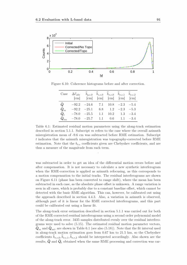
6.2 Evaluation with L-band data 91
0 0.2 0.4 0.6 0.8 10
2
4
6
8x 10
4
|γ|
Cou
nts
InitialCorrected/No TopoCorrected/Topo
Figure 6.10: Coherence histograms before and after correction.
Case ∆rabs by,ǫ,0 bz,ǫ,0 bx,ǫ,0 bx,ǫ,1 bx,ǫ,2[cm] [cm] [cm] [cm] [cm] [cm]
Q −92.2 −24.6 7.1 10.8 −2.3 −5.4
Qm −92.2 −25.1 6.8 1.2 −2.3 −5.3
Qt −78.0 −25.5 1.1 10.2 1.3 −3.4
Qtm −78.0 −25.7 1.1 0.6 1.1 −3.4
Table 6.1: Estimated residual motion parameters using the along-track estimationdescribed in section 5.1.1. Subscript m refers to the case where the overall azimuthmisregistration mean of -9.6 cm was subtracted before RME estimation. Subscriptt indicates that the azimuth misregistration was topography-corrected before RMEestimation. Note that the bx,ǫ coefficients given are Chebyshev coefficients, and arethus a measure of the magnitude from each term.
.
was subtracted in order to get an idea of the differential motion errors before andafter compensation. It is not necessary to calculate a new synthetic interferogramwhen the RME-correction is applied as azimuth refocusing, as this corresponds toa motion compensation to the initial tracks. The residual interferograms are shownon Figure 6.11 (phase has been converted to range shift), where the mean has beensubtracted in each case, as the absolute phase offset is unknown. A range variation isseen in all cases, which is probably due to a constant baseline offset, which cannot bedetected with the basic RME algorithm. This can, however, be calibrated out usingthe approach described in section 4.4.3. Also, a variation in azimuth is observed,although part of it is linear for the RME corrected interferograms, and this partcould be calibrated out using a linear fit.
The along-track error estimation described in section 5.1.1 was carried out for bothof the RME-corrected residual interferograms using a second order polynomial modelof the along-track error. 3435 samples distributed evenly over the residual interfero-grams were used to solve (5.15). The estimated residual motion parameter vectors,Qm and Qmt, are shown in Table 6.1 (see also (5.18)). Note that the fit interval usedin along-track motion estimation goes from 0.67 km to 21.5 km, so the Chebyshevcoefficients bx,ǫ,0, bx,ǫ,1, bx,ǫ,2 should be interpreted accordingly. Also shown are theresults, Q and Qt obtained when the same RME processing and correction was car-

92 Experimental Evaluation
Ran
ge [k
m]
Uncorrected [m]
0 5 10 15 200
1
2
3
4
5
6
−0.1
−0.05
0
0.05
0.1
Ran
ge [k
m]
Corrected, No Topo [m]
0 5 10 15 200
1
2
3
4
5
6
−0.1
−0.05
0
0.05
0.1
Ran
ge [k
m]
Azimuth [km]
Corrected, Topo [m]
0 5 10 15 200
1
2
3
4
5
6
−0.1
−0.05
0
0.05
0.1
Int.
Figure 6.11: Residual interferograms (converted to range shift) after subtraction ofsynthetic interferogram. (top) No RME correction, (middle) RME corrected with-out topographic misregistration compensation, (bottom) RME-corrected with topo-graphic misregistration compensation. In all cases, the mean has been subtracted asthe absolute phase offset is unknown.

6.2 Evaluation with L-band data 93
ried out, but with the difference that the mean azimuth misregistration of -9.6 cmwas not subtracted before RME estimation. It is seen that the −9.6 cm centime-ter azimuth misregistration is accurately modeled by bx,ǫ,0 in each case, with minorvariations of less than 5 mm in the other parameters.
Looking at the difference in the parameters estimated with and without topographycompensation (i.e, Qm vs. Qmt) a 14.2 cm difference in ∆rabs, the main part ofwhich is probably a phase ambiguity of 2π (equivalent to 12 cm) with the L-bandwavelength of 24 cm. This still leaves a difference of 2.2 cm, but also variations ofseveral centimeters in the other parameters are seen, noticably bz,ǫ,0 which changesby 6 cm. Some of this can be explained by the difference in the estimated differen-tial motion errors (see Figure 6.7), but the mean difference between the estimatedvertical cross-track motion corrections with and without topography compensationsare only 7 mm, so this does not explain all. It was attempted to use a higher orderpolynomial model for the residual along-track error, but the estimated bx3 was only7 mm, with little changes in the other parameters. When comparing the estimatedconstant differential motion error (by,ǫ,0, bz,ǫ,0) to the range misregistration with sim-ulated topography contribution subtracted (bottom of Figure 6.6) there appears tobe an inconsistency. The constant differential motion error should be visible in therange misregistration at the start of the image. With the values of (by,ǫ,0, bz,ǫ,0) inTable 6.1 (Qt), a range misregistration of 16 cm is expected, but from Figure 6.6,the observed misregistration at near range is approximately -10 cm. This suggeststhat the constant baseline offset and absolute phase error is modeled incorrectly.An obvious way of doing this is to use the range misregistration in the absolutephase estimation [27]. However more work is needed to integrate this with the along-track estimation. It was attempted to use the residual range misregistration image(Figure 6.6 bottom) as input to the along-track error estimation instead of the resid-ual interferogram (5.12). In this case, an absolute phase offset was not estimated,and the resulting estimates were by,ǫ,0 = 0.2 cm, bz,ǫ,0 = 12.0 cm, bx,ǫ,0 = 0.6 cm,bx,ǫ,1 = 0.8 cm, and bx,ǫ,2 = −4.6 cm. These values should be compared to (Qtm) inTable 6.1. The estimated along-track motion using the residual range registration isclose to the one estimated using the residual interferogram. However, the constantbaseline offset is off, and further work is needed to analyze this.
Using the estimated motion parameters of Table 6.1, a final vertical motion cor-rection can be calculated according to (5.21), and this shown on Figure 6.12. Thecross-track correction bzǫ is a relative correction with respect to the inital RME-estimated cross-track errors on Figure 6.7, and the estimated constant baseline offsethas been added. The motion correction was implemented here as a simple phasecorrection of the RME-corrected residual interferograms to obtain final residual in-terferograms. Another approach would be to repeat the focusing done after the initialRME estimation, but using now the final residual motion estimate. This was notdone for these data, but in the C-band case, a complete refocusing using correctednavigation data was performed, see Section 6.3.
The final corrected residual interferograms should ideally be perfectly flat if themotion errors were estimated correctly and the external DEM was perfect. Theactual residual interferograms are shown in Figure 6.13, where it is the absolutevalue of the residual interferograms (converted from phase to range) that is plottedto illustrate the differences. Except for the temporal+volume decorrelated areas (seeFigure 6.4), the final deviations from the synthetic interferogram are below 2.5 cm in

94 Experimental Evaluation
0 5 10 15 20 25
−0.2
−0.1
0
0.1
0.2
[m]
No TopoTopo−corrected
0 5 10 15 20 25−0.05
0
0.05
0.1
0.15
Azimuth [km]
[m]
No TopoTopo−corrected
bx,ǫ
bz,ǫ,0 + bz,ǫ
Figure 6.12: Final motion correction estimated by the along-track error estimation.
both the topography-compensated and the non-compensated case. The topography-compensated interferogram seems to be slightly flatter than the non-compensated,especially at the left edge and around 5 km azimuth. We observe from Figure 6.5that the latter position is also where significant maximum topographic correction wasapplied. Only in the top right part of the image, the non-compensated interferogramis slightly flatter. The RMS value of the residual phase deviation (if we do notcount in the large incoherent areas) is equivalent to 1.3 cm with the topographiccompensation and 1.4 cm without, so this is a slight improvement. Part of thisvariation could be due to atmospheric effects. As mentioned in section 4.1.2, thetypical RMS range shifts from atmospheric effects lie in the range 2 mm to 1.7 cmat C-band. If the same applies at L-band, this could explain some of the residualRMS variation. The final corrected interferogram phases were also inverted to terrainheight and compared to the SRTM DEM. Of course the data have been correctedusing this DEM, but this gives an idea of the high-frequency differences. In thiscase, the RMS terrain height difference, compared to the external DEM was 3.4 mwithout topography compensation and 3.2 m with topography compensation. In [37]it is mentioned that the RMS height noise on the SRTM C-band DEM is on theorder of 3 m, so results better than this cannot be expected.
To compare the along-track correction method with another method for interferogramcalibration, a simpler DEM calibration was performed on the RME-corrected residualinterferograms. Here the constant baseline offset was estimated as described in 4.4.3,and a mean linear phase in azimuth was subtracted. This approach has also beenused in [38]. Converting these calibrated phases to terrain height, RMS values of3.6 m (without topographic correction) and 3.4 m (with topographic correction)were obtained. A similar DEM calibration can also be performed on the non-RME

6.3 Evaluation with C-band data 95
Ran
ge [k
m]
Without Topographic Correction [m]
0 5 10 15 200
2
4
6
0
0.005
0.01
0.015
0.02
0.025R
ange
[km
]
With Topographic Correction [m]
Azimuth [km]0 5 10 15 20
0
2
4
6
0
0.005
0.01
0.015
0.02
0.025
Figure 6.13: Absolute value of final corrected residual interferograms (converted torange shift) after RME-estimation and along-track correction, (top) without topo-graphic compensation, (bottom) with topographic compensation. These should becompared 6.11
corrected interferogram, and in this case, the RMS terrain height deviation from theexternal DEM becomes 5.7 m, so the main improvement comes from the initial RMEcorrection.
6.3 Evaluation with C-band data
6.3.1 Inital processing
For the C-band data, only the Gulfstream GIII P-code GPS data were available forrefining the INU data before initial focusing (see section 6.1). A speckle correla-tion coregistration (using the emidif program) of the initially focused data, showedrange misregistrations of up to 5 m and azimuth misregistrations of up to 12 m.The emidif misregistration estimates were used in the trctune program, which cal-culates a polynomial differential motion estimate (see section 4.4.1 and [30]). Themisregistrations and estimated polynomial baseline corrections are shown in Figure6.14, together with the horizontal and vertical baseline components as estimated fromthe polynomially corrected navigation. On Figure 6.15 is shown the variation of theparallel and perpendicular baselines components. These are small, as the desiredbaseline for these two maps was 0 m.

96 Experimental Evaluation
0 20 40 60 80 100-15
-10
5
0
5
[m]
Mean Misregistration
RangeAzimut
0 20 40 60 80 100-20
-15
-10
-5
0
5
10
[m]
Polynomial Baseline Correction
0 20 40 60 80 100-10
-5
0
5
Azimuth [km]
[m]
Baseline
h
x
y
y
z
z
Figure 6.14: Navigation data for fl045 C-band data, (top) Mean range and azimuthmisregistration obtained from speckle correlation, (middle) estimated polynomialbaseline correction, (bottom) Final baseline estimate.

6.3 Evaluation with C-band data 97
0 20 40 60 80 100−5
0
5
10Parallel baseline variation
Azimuth [km]
Par
. bas
elin
e [m
]
Near rangeFar range
0 20 40 60 80 100−10
−5
0
5Perpendicular baseline variation
Azimuth [km]
Per
. bas
elin
e [m
]
Near rangeFar range
Figure 6.15: Parallel and perpendicular baselines for fl045, from the navigation datacorrected using polynominal baseline correction.
The polynomial baseline correction was used to correct the navigation data of image 2(m0841), which was then refocused. After refocusing, the residual misregistrationswere below 1 m, which is sufficient for interferogram generation, application of SDC,and subsequent RME estimation.
The amplitude, interferogram phase, and coherence images, generated using 11x11looks, are shown in Figure 6.16, together with the SRTM DEM of the area andthe synthetic interferogram generated using this DEM and the motion data. Themean coherence in the image, excluding the large decorrelated ocean areas, is 0.54,but this is most likely due to decorrelation in vegetated areas, as the images wereacquired in July. The coherence over vegetated areas is generally lower at C-bandthan at L-band, due to the smaller wavelength. Comparing the actual interferogramto the synthetic interferogram, it is seen that the expected (i.e. the synthetic) phasevariations are small compared to the observed variations, which are most probablycaused by differential motion errors.
6.3.2 SDC processing
The azimuth and range misregistration estimation was performed with the spectraldiversity coregistration method, with the same parameters and steps as described in6.2.2. The resulting misregistration images are shown on Figure 6.17. The observedmisregistration is the residual after the initial third order polynomial motion errorestimation using speckle correlation, so low order motion errors have been removed(see Figure 6.14). However a higher-order residual azimuth misregistration signal

98 Experimental Evaluation
Azimuth [km]
Ran
ge [k
m]
0 10 20 30 40 50 60 70 80 900
2
4
6
8
b
Azimuth [km]
Ran
ge [k
m]
0 10 20 30 40 50 60 70 80 900
2
4
6
8
0
π
−π
∆
Azimuth [km]
Ran
ge [k
m]
0 10 20 30 40 50 60 70 80 900
2
4
6
8
0
0.5
1
Azimuth [km]
Ran
ge [k
m]
0 20 40 60 800
2
4
6
8
−50
0
50
Azimuth [km]
Ran
ge [k
m]
0 10 20 30 40 50 60 70 80 900
20
40
60
80
0
π
−π
Figure 6.16: fl045 C-band data after initial focusing and 11x11 multilook, fromtop down: Amplitude, interferometric phase, coherence, SRTM DEM (converted toheight over mocom reference surface), synthetic interferogram from SRTM DEM.

6.3 Evaluation with C-band data 99
Azi
mut
h [k
m]
Range [km]
Azimuth Misreg [m]
0 2 4 6 8
0
10
20
30
40
50
60
70
80
90
−1
−0.8
−0.6
−0.4
−0.2
0
0.2
0.4
0.6
0.8
1
Range [km]
Range Misreg [m]
0 2 4 6 8
0
10
20
30
40
50
60
70
80
90
−1
−0.8
−0.6
−0.4
−0.2
0
0.2
0.4
0.6
0.8
1
Figure 6.17: fl045 misregistrations estimated by SDC, (left) Azimuth, (right) Range.

100 Experimental Evaluation
varying between -1 m and 1 m is seen, overlayed with smaller faster variations. Therange misregistration also shows a slow variation, but here the variation is from -0.5m to 0.5 m. The observed misregistrations are likely due to motion errors that couldnot be modeled by the third-order polynomial because of the long scene length.
6.3.3 RME estimation
The RME estimation was carried out as for the L-band case (section 6.2.3), ex-cept that a mean azimuth misregistration was not subtracted, since this had alreadybeen removed by the initial polynomial motion error estimation. Topography com-pensation was also carried out to improve the estimates, but, unlike the L-bandcase (Figure 6.7), the simulated topography contribution was small compared to theoverall estimated error, which is shown on Figure 6.18.
0 20 40 60 80 100−1.5
−1
−0.5
0
0.5
Azimuth [km]
[m]
by,ǫbz,ǫ
Figure 6.18: fl045 residual motion errors as estimated by the RME algorithm.
It can be seen from Figure 6.18 that the major variation in the residual error isa slow periodic error on the vertical coordinate, but past 60 km in azimuth, bothestimates seem to drift towards negative values. This could be due to the fact thatthe RME algorithm separation of vertical and horizontal cross-track errors becomesill-conditioned here (see section 4.4.2), since there are large water areas where nomisregistration estimates are available. These are excluded from the estimation,based on a coherence mask, and on Figure 6.19 is shown the condition number ofthe HTH matrix used at each azimuth position in the RME estimation (4.51). Thecondition number is seen to increase tenfold over the mentioned areas, comparedto the rest of the image. Further work is needed to increase the RME estimationstability in such cases.
As the estimated residual errors vary significantly compared to the the range reso-lution, the slave image (m0841) navigation data were corrected with the estimatedresidual error and the image refocused, as described in 4.5. After this processing, anew SDC misregistration estimation was carried out in both range and azimuth, theresults of which are shown on Figure 6.20.
Noting the change of scale compared to Figure 6.17, the residual misregistrationhas been significantly improved, and the remaining azimuth misregistration is highfrequency in nature. The rather large variations of up to 0.2 m are due to thesimulated topographic misregistration that was subtracted before RME estimationand has therefore not been corrected. In the range misregistration, a slow residual

6.3 Evaluation with C-band data 101
0 20 40 60 80 10010
1
102
103
104
Azimuth [km]
HTH
Con
ditio
n N
umbe
r
Figure 6.19: Condition number for the HTH matrix used in RME estimation forfl045.
error of up to 15 cm is seen. This is likely due to along-track induced errors. Past70 km, the range misregistration drifts off significantly, which might be due to largeresidual along-track errors, but is most likely due to the conditioning problems ofthe RME estimation mentioned previously. The latter hypothesis is supported bythe fact that the initial azimuth misregistration image (Figure 6.17) does not showespecially large values past 70 km compared to the rest of the image.
Since misregistration errors of up to 1 m has been corrected by the RME correction,an improvement in coherence is expected. The coherence histograms of the uncor-rected and the RME-corrected interferograms are shown on Figure 6.21, where thelarge water areas have been excluded from the calculation. A notable improvementis seen in the high end, but a large number of low-coherent pixels are still present,probably due to the temporal decorrelation of vegetated areas at C-band.
6.3.4 Along-track error estimation
As mentioned in the previous section, the RME-estimated cross-track errors werecorrected by modifying the navigation data and refocusing. After this refocusing, anew interferogram was generated and unwrapped, as described in 6.2.4. The syntheticinterferogram was then subtracted to form a residual interferogram for use in along-track error estimation. Since the RME correction was carried out by correcting thenavigation data, a new synthetic interferogram was calculated from the correctednavigation data. Due to the small baseline used for this scene (see Figure 6.14),the variation of the interferometric shift in the synthetic interferogram is only a fewcentimeters in most of the image, which is small compared to the observed rangemisregistrations. Therefore, an along-track error estimation was also attempted,using the range misregistration image instead of the residual interferogram. In thiscase, no constant range offset was estimated, since the range misregistration estimateis unambiguous. It is interesting to note that with this approach, no external DEMis needed. 14000 samples of the residual interferogram/range registration imagewere used in all cases, distributed evenly over the first 60 km of the scene, due tothe RME estimation problems mentioned in section 6.3.3. The estimated residualmotion parameters are given in Table 6.2, where both a second- and a third-orderalong-track motion model has been used. The differences in the estimated residualmotion parameters are only a few centimeters, which is small compared to the overall

102 Experimental Evaluation
Azi
mut
h [k
m]
Range [km]
Azimuth Misreg [m]
0 2 4 6 8
0
10
20
30
40
50
60
70
80
90
Range [km]
Range Misreg [m]
0 2 4 6 8
0
10
20
30
40
50
60
70
80
90
−0.2
−0.15
−0.1
−0.05
0
0.05
0.1
0.15
0.2
−0.2
−0.15
−0.1
−0.05
0
0.05
0.1
0.15
0.2
In
Figure 6.20: SDC estimates of residual misregistrations observed after RME estima-tion and correction of navigation data.

6.3 Evaluation with C-band data 103
0 0.2 0.4 0.6 0.8 10
1
2
3
4
x 104
|γ|
Cou
nts
UncorrectedCorrected
Figure 6.21: Coherence histograms for fl045, before and after basic RME-estimationand refocusing.
Case ∆rabs by,ǫ,0 bz,ǫ,0 bx,ǫ,0 bx,ǫ,1 bx,ǫ,2 bx,ǫ,3[cm] [cm] [cm] [cm] [cm] [cm] [cm]
Qp2 6.2 −1.1 −13.0 −2.3 12.5 −6.0 -Qp3 6.2 −1.1 −13.2 −2.3 13.0 −6.0 0.4
Qr2 - 1.4 −11.6 −1.8 10.8 −5.3 −Qr3 - 1.4 −11.6 −1.8 10.7 −5.3 0.0
Table 6.2: Estimated residual motion parameters for fl045 using the along-trackestimation described in section 5.1.1, with both second and third order along-trackerror model. Subscript p means that that the residual interferogram was used foralong-track estimation, while r indicates that only the range registration was used.Note that the bx parameters are given as Chebyshev coefficients. The fit interval isfrom 0 km to 60 km.
.

104 Experimental Evaluation
values. Also it is seen that a second order along-track motion model seems sufficientto model the observed residual phase and misregistrations, as the estimated residualmotion parameters change by less than 5 mm by adding a third order term to thealong-track motion model (Qp3 and Qr3).
Using the estimated second-order along-track motion parameters of Table 6.2, a fi-nal vertical motion correction was calculated according to (5.21), and this is shownon Figure 6.22 for the fit interval from 0 to 60 km. The correction bz,ǫ is a rela-tive correction with respect to the inital RME-correction bz,ǫ on Figure 6.18, andthe estimated constant baseline offset has been added. The difference between thecross-track motion estimates obtained using the external DEM, and the estimatesobtained using the range misregistration is no more than two centimeters, except forthe constant horizontal offset, which is slightly larger. To illustrate the along-trackestimation, the residual interferogram before along-track correction is shown on Fig-ure 6.23 together with the phase correction calculated from the estimated verticalerror bzǫ(x) and the estimated constant baseline offset. It is seen that there is goodagreement from 0 to 60 km, for which the along-track motion model has been fitted.
0 10 20 30 40 50 60
−0.2
−0.1
0
0.1
0.2
[m]
IFCoreg
0 10 20 30 40 50 60−0.15
−0.1
−0.05
0
0.05
Azimuth [km]
[m]
IFCoreg
bx,ǫ
bz,ǫ,0 + bz,ǫ
Figure 6.22: fl045 final motion correction, as estimated by the 3rd-order along-trackerror estimation. The solid blue curves were estimated using the external DEM,whereas the dashed red curves were obtained using only the range misregistrationfor along-track error estimation.
After the along-track motion estimation, the slave image navigation data were cor-rected in both along-track and cross-track coordinates using the motion correctionestimated from the residual interferogram with the second-order along-track motionmodel, Qp3. Then the image was refocused, following which a final interferogram

6.3 Evaluation with C-band data 105
Azi
mut
h [k
m]
Range [km]
Residual IF Shift [m]
0 2 4 6 8
0
10
20
30
40
50
60
70
80
90
-0. 2
-0.15
-0. 1
0.05
0
0.05
0.1
0.15
0.2
Range [km]
Correction IF Shift [m]
0 2 4 6 8
0
10
20
30
40
50
60
70
80
90
-0. 2
-0.15
-0. 1
0.05
0
0.05
0.1
0.15
0.2
Fit in
terv
al
Figure 6.23: Residual interferogram (converted to range shift) and estimated correc-tion with a 3rd-order along-track motion model. Note that the model has only beenfitted from 0 to 60 km in azimuth.

106 Experimental Evaluation
was calculated and unwrapped. Spectral diversity range and azimuth misregistra-tion estimation were also carried out, and the residual azimuth misregistration wasvirtually unchanged compared to the residual azimuth misregistration of the basicRME-corrected image of Figure 6.20. This is as expected, since the misregistrationfrom the applied along-track correction balances out with the misregistration inducedby the cross-track correction.
In the range misregistration image, a mean offset of 2.6 cm is still present, the reasonfor which is not known. It might be related to the fact that the data were correctedusing the final motion parameters estimated from the residual interferogram. Herean absolute range offset of 6.2 cm (which might include an N · 2π phase ambiguity,corresponding to N · 2.83 cm) was estimated, but this has not been applied to thenavigation data correction, as it is not possible to correct it this way. Such a constantoffset is easy to calibrate out, however. A final residual interferogram was alsocalculated by subtracting from the final interferogram the synthetic interferogramcalculated from the final navigation data. In this case, an offset of 2.7 cm was seen.In Figure 6.24 the absolute variation of the residual range misregistration is shown,together with the absolute residual interferogram variation. In both cases, the meanvalue has been subtracted before taking absolute values. It is seen that the slowvariation in the residual phase and misregistration (Figures 6.20 and 6.23) has beenremoved, and the final variation of the residual interferometric shift is below 2 cmover the entire fit area from 0 to 60 km. The RMS value of the residual interferometricshift is 7 mm. This is on the order of the RMS value typically seen from atmosphericeffects (see section 4.1.2). The appearance of the range misregistration image isprobably due to noise in the SDC estimate as well as topography, which is includedin the range registration.
To obtain independent verification of the final misregistration estimate, an emidif
speckle correlation using 24× 256 patches across the image was carried out betweenthe master and the final corrected slave image. Azimuth profiles (averaged in therange direction) of the emidif misregistration estimates are compared to the SDCestimates on Figure 6.25. For the fit area from 0 to 60 km, the mean range misregis-tration of 2.6 cm is observed on both the emidif and SDC estimates, with variationsfrom this value of less than two centimeters. Past 60 km, the range misregistrationsincrease due to the conditioning of the RME estimate in this area (see section 6.3.3).
In the azimuth misregistration, it is seen that the emidif misregistration estimatesare undersampled compared to the SDC estimates. The residual mean azimuthmisregistrations of up to 5 cm are due to the topography-induced azimuth misreg-istrations, which are not corrected with the approach in this work. This could bedone if topography-dependent motion compensation was carried out, as mentionedin 5.2.4.
6.4 Discussion
For the L-band scene treated in section 6.2 it was seen that the major part of thedifferential motion error and related azimuth misregistration was corrected by thebasic RME algorithm (section 4.4.2), and only a slight improvement was achievedby using the proposed along-track residual motion correction (section 5.1.1) insteadof a standard calibration method. The improvement from applying the topography

6.4 Discussion 107
Azi
mut
h [k
m]
Range [km]
Range Misreg. [m]
0 2 4 6 8
0
10
20
30
40
50
60
70
80
90
0
0.005
0.01
0.015
0.02
0.025
0.03
0.035
0.04
0.045
0.05
Range [km]
Residual IF shift [m]
0 2 4 6 8
0
10
20
30
40
50
60
70
80
90
0
0.005
0.01
0.015
0.02
0.025
0.03
0.035
0.04
0.045
0.05
Figure 6.24: Absolute values of residual range misregistration and residual interfer-ogram (converted to range) after final motion data correction and refocusing. Themean value of 2.6 cm has been subtracted from the range registration, and a meanof 2.7 cm has been subtracted from the residual interferograms. The means weresubtracted before taking absolute values.

108 Experimental Evaluation
0 20 40 60 80 1000
0.1
0.2
[m]
Range Misregistration
0 20 40 60 80 100-0. 1
-0.05
0
0.05
0.1
Azimuth [km]
[m]
Azimuth Misregistration
SDCEMIDIF
SDCEMIDIF
∆
Figure 6.25: Comparison of final misregistration estimates from speckle correlation(emidif) and spectral diversity (SDC).
compensation (section 5.2.4) was also slight, however it could be observed in the finalresidual interferograms. In all cases, the RMS deviations of the residual devationswere comparable to the expected deviations of the external SRTM DEM, to which thedata were calibrated. More work is needed to improve the estimate of the absolutephase and the constant differential motion error, using the range misregistrationestimate.
For the long C-band scene processing described in section 6.3, it was seen that theRME algorithm again compensated the major part of the differential motion error.However, a residual quadratic error was seen in both the range registration and theresidual interferometric shift. Here, the proposed along-track motion estimation al-gorithm accurately compensated for this, except for a 2.6 cm offset that was observedin both the final range misregistration and interferogram. This is probably relatedto a constant phase offset between the two images, and is easily calibrated out. Oth-erwise, the observed variations of the residual interferograms was below 2 cm andnot systematic in nature. This is true for the first 60 km of the scene. Past 60 km,the observed range misregistration could not be corrected, but this was probably dueto stability problems in the RME algorithm caused by the narrow swath availablehere due to the ocean. More work is needed to improve the stability of the RMEalgorithm over such areas. It might be possible to constrain the RME estimate us-ing the observed range misregistration, or by extrapolation of the estimated RMEderivatives from neighbouring azimuth positions where a wider swath is available.

Chapter 7
Conclusions
The present thesis has dealt with two aspects of motion errors in airborne SAR,propeller induced motion errors and residual motion estimation in repeat track in-terferometry.
7.1 Vibration analysis
In Chapter 3, the impact of propeller-induced vibration on the SAR impulse responsewas examined through spectral analysis and point target simulations using motiondata measured on a C-130 heavy turboprop aircraft, a Piper PA31 light turpopistonaircraft, and, for reference a Gulfstream GIII jet aircraft. The overall conclusionis that the estimated physical vibration amplitudes above 5-10 Hz do not seem tolead to unacceptable sidelobes in the SAR impulse responses. However, it was foundthat aliasing of the measured propeller-induced vibration in the motion sensor could,when performing motion compensation, lead to unacceptable spurious sidelobe levelsof up to −26 dB in a high-resolution X-band system if a 50 Hz motion sensor wasused in a C-130. However, the applied motion sensor was capable of delivering 200Hz motion data, for which case there did not seem to be any unacceptable sidelobelevels.
For the Piper PA31 case, only 50 Hz motion data were collected, and in this case,all the observed motion above some 5 Hz was seen to be aliased. The simulatedsidelobe levels for this case were below −30 db, but such sidelobes could be removedby low-pass filtering the motion data before applying them in motion compensation.Using a higher frequency motion sensor would also alleviate the problem.
For the GIII Gulfstream jet aircraft, there were no high frequency vibrations sig-nificant enough to cause sidelobes above the nominal Hamming-weighted impulseresponse.
7.2 Residual motion errors in RTI
In the second part of this thesis, an existing differential motion error estimationalgorithm, the RME algorithm, has been implemented in MATLAB and tested onEMISAR data. As a prerequisite for this, it was also necessary to implement the

110 Conclusions
Spectral Diversity (SDC) algorithm for misregistration estimation. The RME al-gorithm integrates the estimated azimuth misregistrations to obtain an estimate ofthe differential cross-track motion error. The principles behind the algorithm is de-scribed in Chapter 4. A strength of the RME algorithm is that is non-parametric,so cross-track motion errors with arbitrary variation can be estimated. However,the algorithm cannot in itself estimate a constant cross-track error, which must beestimated using tie-points or an external DEM.
In Chapter 5, two improvements to the RME algorithm were proposed. The im-provement which seems most significant is a scheme to correct for errors in theRME estimate due to along-track motion errors. Differential along-track motion er-rors cause azimuth misregistrations which in the RME algorithm are interpreted,incorrectly, as due to a cross-track velocity error. The proposed algorithm uses anexternal digital elevation model (DEM) to estimate the errors due to along-trackmotion. The along-track error is modeled as having a polynomial variation, but thisis not a significant limitation, as only slowly varying along-track errors will affectthe RME estimate significantly, and a fast variation in the along-track error can beignored. Using the estimated along-track error, the cross-track motion data can thenbe corrected for the errors initially induced by the RME estimation, without affect-ing the corrected azimuth misregistration. Together with the along-track motion,the constant cross-track offset (see above) and a phase offset is also estimated.
Another error source in the RME algorithm is azimuth misregistrations caused byuncompensated topography coupling with sensor cross-track velocities. A method isproposed for compensating this error contribution in the RME algorithm using anexternal DEM. The proposed method is simple and does not correct the azimuthmisregistrations induced by the topography. This can only be achieved using to-pography dependent motion compensation, which complicates the SAR processingconsiderably.
In Chapter 6, the RME algorithm has been applied to two different scenes, an L-band scene with an azimuth length of 22.5 km and a C-band scene with a lengthof 100 km. The proposed modifications to the RME algorithm were then appliedto see if they could improve the results. Both of the proposed modifications requirean external DEM, and the DEM used in this work is the Shuttle Radar TopographyMission (SRTM) DEM.
In the L-band scene, kinematic GPS data were available, but a fast varying azimuthmisregistration motion error of up to ±0.5 m was observed, the main part of whichwas probably due to an uncompensated delay between radar data and navigationdata for both images. These variations were corrected by the RME algorithm, and aslowly varying residual phase of 10-15 cm could then be modeled by the along-trackmotion estimation. This left a residual RMS phase variation equivalent to 1.4 cmbetween the corrected interferogram and the synthetic interferogram generated fromthe DEM. This was shown to be consistent with the expected DEM noise from theexternal DEM. Compared to a standard DEM calibration (estimating and correctinga constant cross-track offset in the range direction and a linear phase in azimuth)of the RME-corrected interferogram, the along-track error estimation method pro-duced slightly better results for the L-band data. The implemented topographicmisregistration correction slightly improved the observed RMS phase variation (af-ter along-track correction) from 1.4 cm to 1.3 cm. However, the estimation of theconstant cross-track baseline error and the absolute phase offset caused problems,

7.3 Acknowledgements 111
which still need further work. It is expected that the range misregistration can beapplied in this case.
In the C-band scene, the RME algorithm also corrected the major part of the differ-ential motion errors, but here a slow varying residual quadratic error of up to 15 cmwas seen on both the residual interferogram and range misregistration. This could beaccurately modeled by the proposed along-track error estimation, leaving a residualerror variation below 2 cm over the 60 km strip to which the data were fitted. It wasalso found that the along-track induced error could alternatively be estimated by theresidual range misregistration to obtain final motion correction estimates within 2cm of the estimates obtained from the residual phase and the DEM. This is interest-ing, as an external DEM is not necessary in this case. However, avoiding an externalDEM is not generally possible if the range misregistration is significantly affected bytopography.
The proposed along-track motion estimation algorithm seems stable, (except for theestimation of the constant baseline offset and absolute phase), and seems to be ableto model succesfully the slow-varying residual motion errors observed after standardRME correction. This could have applications in differential interferometry andrepeat pass DEM generation in cases where a rough DEM of the imaged area isavailable beforehand, and the stationary parts of the scene can be used for RMEestimation.
Further investigations are probably needed to verify the merits of the proprosedtopography compensation for the RME algorithm although it seems to offer a slightimprovement in the L-band case. This could be examined using a scene with moretopography, but this was not done.
7.3 Acknowledgements
I wish to thank Kristian Keller, formerly at the National Survey and Cadastre (KMS),for supplying the PA31 navigation data as well as for lending out their EGI unit.Also, thanks to Andreas Reigber for having me as a guest at the Technical Universityof Berlin, and to Johan Mohr for assistance in using the sarif SAR processor andassociated tools. Steen Savstrup Kristensen is thanked for his help in recoveringraw EMISAR data from damaged tapes, Sten Schmidl for moral support and for hisassistance before and during the C-130 EGI data collection. Finally, thanks to mysupervisors, Erik Lintz Christensen and Jørgen Dall for always taking time out oftheir busy schedule when necessary.


Bibliography
[1] Christensen, E.L. (editor), “SAR++ System Design Report,” Tech. Rep. R693,Ørsted•DTU - Electromagnetic Systems, 2000.
[2] Reigber, A. and Papathanassiou, K.P., “Correction of residual motion errorsin airborne repeat-pass interferometry,” Geoscience and Remote Sensing Sym-posium, 2001. IGARSS ’01. IEEE 2001 International, vol. 7, pp. 3077–3079,2001.
[3] Kirk, J.C., “Motion compensation for synthetic aperture radar,” IEEE Trans-actions on Aerospace and Electronic Systems, vol. AES-11, no. 3, pp. 338–48,1975.
[4] Fornaro, G., “Trajectory deviations in airborne SAR: analysis and compensa-tion,” IEEE Transactions on Aerospace and Electronic Systems, vol. 35, no. 3,pp. 997–1009, 1999.
[5] Carrara, W.G. and Goodman, R.S. and Majewski, R.M, Spotlight SyntheticAperture Radar: Signal Processing Algorithms. Artech House Inc., 1995.
[6] Curlander, J.C. and McDonough, R.N., Synthetic Aperture Radar - Systems andSignal Processing. John Wiley & Sons, 1991.
[7] Bamler, R., “A comparison of range-Doppler and wavenumber domain SARfocusing algorithms,” Geoscience and Remote Sensing, IEEE Transactions on,vol. 30, no. 4, pp. 706 –713, 1992.
[8] Klauder, J.R. and Price, A.C. and Darlington, S. and Aldersheim, W.J, “TheTheory and Design of Chirp Radars,” Bell System Technical Journal, vol. 39,no. 4, pp. 745–808, 1960.
[9] Klein, J.D. and Hensley, S. and Madsen, S.N. and Webb, F.H., “Results of 1993repeat-pass SAR interferometry experiments,” Geoscience and Remote Sens-ing Symposium, 1994. IGARSS ’94. Surface and Atmospheric Remote Sensing:Technologies, Data Analysis and Interpretation., International, vol. 1, pp. 295–297 vol.1, 1994.
[10] Grewal, Mohinder S. and Weill, Lawrence R. and Andrews, Angus P., GlobalPositioning Systems, Inertial Navigation, and Integration. John Wiley & Sons,Inc., 2001.
[11] Hoogeboom, P. and Snoeij, P. and Koomen, P.J. and Pouwels, H., “ThePHARUS project, results of the definition study including the SAR testbed

114 BIBLIOGRAPHY
PHARS,” IEEE Transactions on Geoscience and Remote Sensing, vol. 30, no. 4,pp. 723–735, 1992.
[12] Horn, R., “E-sar - The Experimental Airborne L/c-band Sar System OfDFVLR,” Geoscience and Remote Sensing Symposium, 1988. IGARSS ’88. Re-mote Sensing: Moving Toward the 21st Century., International, vol. 2, pp. 1025–1026.
[13] Kusk, A. and Dall, J. and Christensen, E.L., “Aircraft Vibrations and NavigationSystem Performance in SAR,” Proceedings, EUSAR 2004, vol. 1, pp. 325–328,2004.
[14] Honeywell Millitary Avionics Division, St. Petersburg, Florida, Prime Item De-velopment Specification for the H764G Embedded GPS Receiver in an INS (EGI)Rev. F, 1995.
[15] Honeywell Military Avionics Division, System Description For Honeywell’s H-764G Block II Embedded Global Positioning System (GPS) Receiver In An In-ertial Navigation System (INS), September 1993.
[16] Honeywell International, Inc., Q-Flex QA2000 Accelerometer Datasheet. Avail-able from http://www.inertialsensor.com/docs/qa2000.pdf.
[17] Majure, R.G., “Demonstration of a ring laser gyro system for pointing andstabilization applications,” Position Location and Navigation Symposium, 1990.Record., pp. 219 –225, 1990.
[18] Stoica, Petre and Moses, Randolph L., Introduction to Spectral Analysis.Prentice-Hall, 1997.
[19] “Personal Communication with Östling and Dammert of Ericsson MicrowaveSystems AB, Airborne Radar Divison, 2004.”.
[20] Östling, D. and Dammert, P.B.G., “Generation and Geocoding of High Resolu-tion SAR Images with the Ericsson SAR/GMTI Experiment System,” Proceed-ings of EUSAR 2004, vol. 2, pp. 941–944, 2004.
[21] Mohr, J. J., Repeat Track SAR Interferometry - An Investigation of its Utilityfor Studies of Glacier Dynamics. PhD thesis, Technical Univeristy of Denmark- Department of Electromagnetic Systems, 1997. LD125.
[22] Hannsen, R., Atmospheric heterogeneities in ERS tandem SAR interferometry.Delft University Press, 1998.
[23] Bamler, R. and Just, D., “Phase statistics and decorrelation in SAR interfero-grams,” Geoscience and Remote Sensing Symposium, 1993. IGARSS ’93. BetterUnderstanding of Earth Environment., International, vol. 3, pp. 980–984, 1993.
[24] Gatelli, F. and Guamieri, A.M. and Parizzi, F. and Pasquali, P. and Prati, C.and Rocca, F., “The wavenumber shift in SAR inferometry,” Geoscience andRemote Sensing, IEEE Transactions on, vol. 32, no. 4, pp. 855 –865, 1994.
[25] Stevens, D.R. and Cumming, I.G. and Gray, A.L., “Options for airborne inter-ferometric SAR motion compensation,” Geoscience and Remote Sensing, IEEETransactions on, vol. 33, no. 2, pp. 409 –420, 1995.

BIBLIOGRAPHY 115
[26] Scheiber, R. and Moreira, A., “Coregistration of interferometric SAR imagesusing spectral diversity,” Geoscience and Remote Sensing, IEEE Transactionson, vol. 38, no. 51, pp. 2179 –2191, 2000.
[27] Madsen, S.N., “On absolute phase determination techniques in SAR interferom-etry,” Proceedings of the SPIE - The International Society for Optical Engineer-ing, vol. 2487, pp. 393–401, 1995.
[28] Bamler, R. and Eineder, M., “Accuracy of Differential Shift Estimation by Cor-relation and Split-Bandwidth Interferometry for Wideband and Delta-k SARSystems,” Geoscience and Remote Sensing Letters, IEEE, vol. 2, no. 2, pp. 151–155, 2005.
[29] Madsen, S.N and Zebker, H., Manual of Remote Sensing, 3rd ed., ch. 6. Imag-ing Radar Interferometry. American Society for Photogrammetry and RemoteSensing, 1997.
[30] Mohr, J. J. and Madsen, S. N., “Parametric Estimation of Time Varying Base-lines in Airborne Interferometric SAR,” Proceedings of IGARSS’96, vol. 1,pp. 677–679, 1996.
[31] Reigber, A. and Prats, P. and Mallorqui, J.J., “Refined estimation of time-varying baseline errors in airborne SAR interferometry,” Geoscience and RemoteSensing Symposium, 2005. IGARSS ’05. Proceedings. 2005 IEEE International,vol. 7, pp. 4799–4802, 2005.
[32] Scheiber, R. and Robert, P., “Origin and correction of phase errors in airbornerepeat-pass SAR interferometry,” Geoscience and Remote Sensing Symposium,2001. IGARSS ’01. IEEE 2001 International, vol. 7, pp. 3114–3116, 2001.
[33] Prats, P. and Reigber, A. and Mallorqui, J.J., “Interpolation-Free Coregistrationand Phase-Correction of Airborne SAR Interferograms,” Geoscience and RemoteSensing Letters, IEEE, vol. 1, no. 3, pp. 188–191, 2004.
[34] Prats, P. and Reigber, A. and Mallorqui, J.J. and Broquetas, A., “Efficient de-tection and correction of residual motion errors in airborne SAR interferometry,”IGARSS 2004. 2004 IEEE International Geoscience and Remote Sensing (IEEECat. No.04CH37612), pp. 992–5 vol.2, 2004.
[35] “http://www.jpl.nasa.gov/srtm/.”
[36] Prats, P. and Reigber, A. and Mallorqui, J.J., “Topography-Dependent MotionCompensation for Repeat-Pass Interferometric SAR Systems,” Geoscience andRemote Sensing Letters, IEEE, vol. 2, no. 2, pp. 206–210, 2005.
[37] Rosen, P.A. and Hensley, S. and Gurrola, E. and Rogez, F. and Chan, S. andMartin, J. and Rodriguez, E., “SRTM C-band topographic data: quality assess-ments and calibration activities,” Geoscience and Remote Sensing Symposium,2001. IGARSS ’01. IEEE 2001 International, vol. 2, pp. 739–741, 2001.
[38] Reigber, A. and Scheiber, R., “Airborne differential sar interferometry: firstresults at L-band,” Geoscience and Remote Sensing, IEEE Transactions on,vol. 41, no. 62, pp. 1516–1520, 2003.


![Index [complements.lavoisier.net] · Subcanopy and Subsurface (AirMOSS) 260–261 airborne sensors AirMOSS 260–261 E‐SAR/F‐SAR/PLMR2, 261–262 and features 260 HyMap 259–260](https://static.fdocuments.in/doc/165x107/5e3275efbac565760d5b4a2e/index-subcanopy-and-subsurface-airmoss-260a261-airborne-sensors-airmoss.jpg)
