1

S A L

Blominvest Working Paper

Research Department

Estimating Real GDP Growth for Lebanon

Prepared by Marwan Mikhael, Michel G. Kamel, and Gaelle Khoury

Authorized for Distribution by Dr. Fadi Osseiran

December 2010

ABSTRACT

This paper presents an econometric framework to estimate quarterly GDP growth for Lebanon

based on a bottom up approach from the demand side. The model relies on a data set of 68

quarterly observations from 1993 to 2009 for ten endogenous variables and two exogenous

variables selected on the basis of their economic and statistical significance. Quarterly GDP figures

are obtained from the annual series using the Chow-Lin disaggregation method. The model derived

is a Vector Autoregressive Model with Exogenous Variables (VARX), a variant of the Vector

Autoregressive Model (VAR) that takes into account both exogenous and endogenous variables.

Our empirical results show robust correlation between the estimate and actual quarterly GDP

figures, indicating the ability of the model to provide a high level of accuracy in estimating real GDP

growth.

JEL Classification Numbers: C51, C32, C13, C82, O53

Keywords: Granger causality, VAR, VARX, impulse response function, and GDP estimate.

Disclaimer: This report is published for information purposes only. The information herein has been compiled from, or based upon sources we

believe to be reliable, but we do not guarantee or accept responsibility for its completeness or accuracy. This document should not be

construed as a solicitation to take part in any investment, or as constituting any representation or warranty on our part. The consequences of

any action taken on the basis of information contained herein are solely the responsibility of the recipient.

Copyright 2010 BLOMINVEST SAL

No part of this material may be copied, photocopied or duplicated in any form by any means or redistributed without the prior written consent

of BLOMINVEST SAL.

2

S A L

Table of Contents

I- Introduction.................................................................................................................................. 3

II- Literature Review ........................................................................................................................ 5

III- GDP Disaggregation in the Case of Lebanon .............................................................................. 6

IV- Choice and Characteristics of Variables ..................................................................................... 8

V- The Vector Autoregressive Model (VAR) .................................................................................. 10

VI- Vector Autoregressive with Exogenous Variables (VARX) ....................................................... 14

VII- Impulse response .................................................................................................................... 18

VIII- Conclusion .............................................................................................................................. 21

References ..................................................................................................................................... 22

Appendix A - VAR Stationarity ....................................................................................................... 24

Appendix B - Vector Autoregressive Model (VAR) ........................................................................ 26

Appendix C - Residual Terms ......................................................................................................... 28

3

S A L

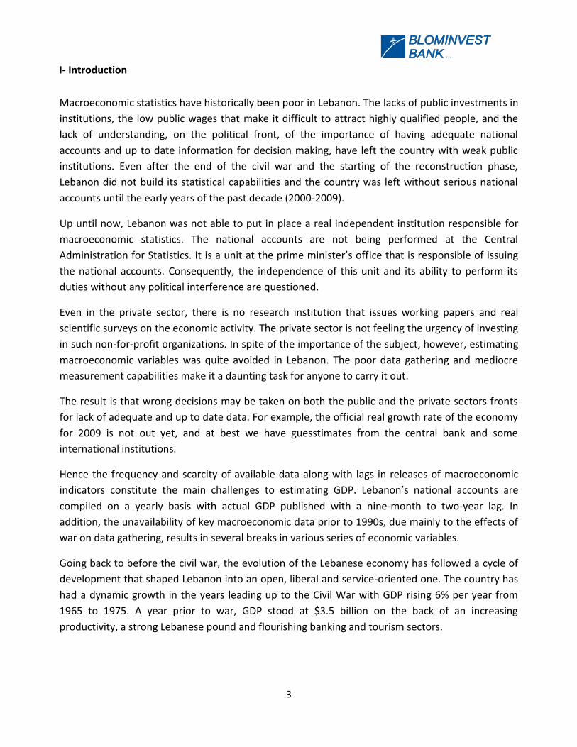
I- Introduction

Macroeconomic statistics have historically been poor in Lebanon. The lacks of public investments in

institutions, the low public wages that make it difficult to attract highly qualified people, and the

lack of understanding, on the political front, of the importance of having adequate national

accounts and up to date information for decision making, have left the country with weak public

institutions. Even after the end of the civil war and the starting of the reconstruction phase,

Lebanon did not build its statistical capabilities and the country was left without serious national

accounts until the early years of the past decade (2000-2009).

Up until now, Lebanon was not able to put in place a real independent institution responsible for

macroeconomic statistics. The national accounts are not being performed at the Central

Administration for Statistics. It is a unit at the prime minister’s office that is responsible of issuing

the national accounts. Consequently, the independence of this unit and its ability to perform its

duties without any political interference are questioned.

Even in the private sector, there is no research institution that issues working papers and real

scientific surveys on the economic activity. The private sector is not feeling the urgency of investing

in such non-for-profit organizations. In spite of the importance of the subject, however, estimating

macroeconomic variables was quite avoided in Lebanon. The poor data gathering and mediocre

measurement capabilities make it a daunting task for anyone to carry it out.

The result is that wrong decisions may be taken on both the public and the private sectors fronts

for lack of adequate and up to date data. For example, the official real growth rate of the economy

for 2009 is not out yet, and at best we have guesstimates from the central bank and some

international institutions.

Hence the frequency and scarcity of available data along with lags in releases of macroeconomic

indicators constitute the main challenges to estimating GDP. Lebanon’s national accounts are

compiled on a yearly basis with actual GDP published with a nine-month to two-year lag. In

addition, the unavailability of key macroeconomic data prior to 1990s, due mainly to the effects of

war on data gathering, results in several breaks in various series of economic variables.

Going back to before the civil war, the evolution of the Lebanese economy has followed a cycle of

development that shaped Lebanon into an open, liberal and service-oriented one. The country has

had a dynamic growth in the years leading up to the Civil War with GDP rising 6% per year from

1965 to 1975. A year prior to war, GDP stood at $3.5 billion on the back of an increasing

productivity, a strong Lebanese pound and flourishing banking and tourism sectors.

4

S A L

In the years that followed the Civil war, Lebanon has entered an era where reliable statistics on the

state of the economy were usually absent. Lebanese economists were sometimes able to compile a

few indicators, but the numbers were often based on incomplete data.

In the aftermath of the war, the advent of the Hariri Government in October 1992, led to the

restoration of the country’s infrastructure and lifted up the economic activity on all levels. Solidere

managed the reconstruction of Beirut’s central business district and the stock market reopened in

January 1996. GDP expanded from $1.3 billion in 1990 to $16.7 billion in 2000.

The private sector was the engine for economic recovery after the war, and till today, it still stands

as the principle pillar for economic growth sustainability through services (mainly tourism, real

estate and banking) sectors that combined, represent 70% of GDP. The economy today, however, is

heavily indebted with gross public debt totaling $54.4 billion and accounting for 139% of GDP.

Political instability poses as well a severe hurdle for economic growth.

In this context, estimating economic growth has a crucial purpose to fill within the large field of

policy making and it represents one of the basic problems of statistical analysis upon which

authorities rely to set the right policies. In this paper, we try to present a general model to obtain

quarterly real GDP growth estimates. Current GDP levels may provide only insufficient information

on future macroeconomic developments. GDP estimates that link near-future growth to current

development, can bridge this gap.

During the conduct of our work, we were faced with two major challenges: the first one was

related to available series of data and the second one was to try to come up with an accurate and

scientific model to estimate real GDP growth rate. For the first challenge we had annual GDP series

going back to just 1993, which does not constitute enough data to build the model. So we had to

transform the annual GDP numbers into quarterly data to increase the size of our sample and to

get real growth rates estimates on a quarterly basis, which does not exist for Lebanon. For the

second challenge, we tried to build our model around a set of variables using a vector

autoregressive (VAR) approach. For variables other than GDP, we had monthly series going back to

1993.

The rest of the paper is organized as follows. Section II and III provide an overview of the different

GDP estimation methods applied worldwide with a focus on the case of Lebanon. Section IV and V,

present a potential Vector Autoregressive Model (VAR) for GDP estimation that was developed in

this paper and address its limitation. Section VI provides a variant of the VAR, a Vector

Autoregressive Model with Exogenous variables (VARX), which offers a better precision in

estimating real GDP and overpass the limitations encountered with the VAR. Section VII describe

the impulse response of real GDP to shocks on various variables. The appendix lay out the complete

details of the specifications used in the empirical application.

5

S A L

II- Literature Review

Disaggregation methods to obtain quarterly GDP from annual GDP have been extensively

considered in econometric and statistical literature. The many proposed solutions have been

reached using one of the following two approaches:

The first one being a method which estimates the disaggregated series (e.g. quarterly GDP) using

information derived only from past and current values of the aggregated series itself (e.g. annual

GDPt; annual GDPt-1). This approach does not involve the use of parameters as no additional

exogenous variables are considered. We distinguish here between non-model based methods,

Polynomial (1988), Lisman & Sandee (1964) and model based methods, Stram & Wei (1986). The

former relies on purely numerical disaggregation technique. An example would be to divide the

annual data into a quarterly figure. This approach is known as linear interpolation and it is mostly

used for stocks disaggregation. Another example of non-model based method, is the Polynomial

method (1988) which converts the annual series to quarterly figures by fitting a polynomial to each

successive set of two points (e.g. GDP2000 and GDPQ1/2001) to derive a smooth path for the

unobserved series. The model-based methods use an ARIMA process.

The second methodology, with more interest for our purposes, consists of a method that presents

a disaggregation scheme (e.g. for quarterly GDP disaggregation) based on information which comes

from the aggregated series itself and also from other exogenous series, called related series (e.g.

consumption of durable goods, volume of exports). The related series are assumed to be known at

the same disaggregation level as the considered disaggregated series (i.e. quarterly GDP in our

case). This approach is model-based and uses correlated time series to provide estimates of the

disaggregated series based on the parameters (𝛽 𝑎𝑛𝑑 𝑢 ) of the aggregated series. The method was

adopted by Friedman (1962), and by Chow and Lin (1971). Variants of it were proposed by Bournay

and Laroque (1979), Fernandez (1981) and Litterman (1983).

Andreas Kladroba (2005) carried out a study to compare different methods for a simulated series

from an ARIMA (1, 1, 1) and showed that Chow-Lin is the most accurate for this relative simulated

series.

Regarding GDP estimation, two methods were developed. The first one consists of developing

indicators relying on a non-model based methodology. This approach was adopted by Carriero and

Marcellino (2010) and by the Conference Board that constructs the Composite Coincident Indicator

(CCI) for the United States as a simple weighted average of selected standardized single indicators.

The second type, adopted in this paper, consists of developing a model-based quarterly estimate of

GDP derived through bottom-up approach based on actual values of the quarterly components

which serve as proxies for selected indicators. There exists the non-parametric method; an example

to cite is the Neural Network with an economic application; and the parametric models. The latter

6

S A L

include the Vector Autoregressive model (VAR) which is adopted in this paper, the Error Correction

Model (VECM), and the Markov Switching Models (MSVAR) which is an updated version of the VAR.

Stochastic models were also built and used such as the Dynamic Stochastic General Equilibrium

(DSGE) model that provides a continuous path for the estimated variable (e.g. provides a graphical

trend for GDP over the whole quarter instead of a stock value).

The European Central Bank uses log-linear approximations to deal with real-time data set and

estimates GDP for the euro area using a VAR model. Braun (1991) uses a Bayesian vector

autoregression (BVAR) to smooth out US production and fill in the missing data for a given quarter.

The Bureau of Economic Analysis (BEA) estimates GDP on an annual and on a quarterly basis. The

first estimate for a certain quarter, namely the “Advance” estimate is done by extrapolation based

on the monthly trends as incomplete data account for about 30% of the advance GDP estimate.

III- GDP Disaggregation in the Case of Lebanon

We estimate GDP for Lebanon from the demand side, relying on indicators and predictors in

different sectors of the economy as proxies to consumption, investment, and trade. The model

proposed is the first GDP estimate model developed for Lebanon.

Other estimates are only indicators for the trend in economic activity. The Banque du Liban (BDL)

and the International Institute of Finance (IIF) have designed indices to measure the evolution of

the country’s economic activity. The former was developed in 1993 and is called “Coincident

Indicator Index”. It relies on eight indicators: electricity production, imports of petroleum,

passengers flows, cement derivatives (all in volume terms), imports and exports, cleared checks,

and broad money. The latter follow the BDL’s approach, and includes five additional indicators: real

growth in credit to the private sector (to substitute for growth in deposits), growth in tourist

arrivals (to substitute for passengers arrivals), real growth in government revenues excluding

grants, real growth in government consumption (current expenditure minus transfers minus

interest payments), and real growth in imports of machinery and equipment. Electricity production

has been excluded because, according to IIF, it does not accurately reflect consumption in Lebanon,

since a significant portion of electricity is derived from private generators. We second the

argument and therefore exclude it from our model.

We used the Chow and Lin approach to disaggregate annual GDP into quarterly levels. The Chow

and Lin solution (1971) has been intensively used in National Statistical Institutes. The reason lies in

the practicality of its procedure and in the natural and coherent solution that the model provides

to the interpolation problem.

7

S A L

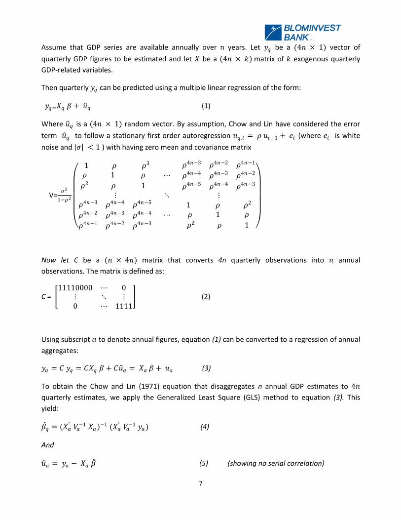
Assume that GDP series are available annually over n years. Let 𝑦𝑞 be a (4𝑛 × 1) vector of

quarterly GDP figures to be estimated and let 𝑋 be a (4𝑛 × 𝑘) matrix of 𝑘 exogenous quarterly

GDP-related variables.

Then quarterly 𝑦𝑞 can be predicted using a multiple linear regression of the form:

𝑦𝑞=𝑋𝑞 𝛽 + 𝑢 𝑞 (1)

Where 𝑢 𝑞 is a (4𝑛 × 1) random vector. By assumption, Chow and Lin have considered the error

term 𝑢 𝑞 to follow a stationary first order autoregression 𝑢𝑞 ,𝑡 = 𝜌 𝑢𝑡−1 + 𝑒𝑡 (where 𝑒𝑡 is white

noise and 𝜎 < 1 ) with having zero mean and covariance matrix

V=𝜎2

1−𝜌2

1 𝜌 𝜌3

𝜌 1 𝜌

𝜌2 𝜌 1

⋯

𝜌4𝑛−3 𝜌4𝑛−2 𝜌4𝑛−1

𝜌4𝑛−4 𝜌4𝑛−3 𝜌4𝑛−2

𝜌4𝑛−5 𝜌4𝑛−4 𝜌4𝑛−3

⋮ ⋱ ⋮𝜌4𝑛−3 𝜌4𝑛−4 𝜌4𝑛−5

𝜌4𝑛−2 𝜌4𝑛−3 𝜌4𝑛−4

𝜌4𝑛−1 𝜌4𝑛−2 𝜌4𝑛−3

⋯

1 𝜌 𝜌2

𝜌 1 𝜌

𝜌2 𝜌 1

Now let C be a (𝑛 × 4𝑛) matrix that converts 4n quarterly observations into 𝑛 annual

observations. The matrix is defined as:

C = 11110000 ⋯ 0

⋮ ⋱ ⋮0 ⋯ 1111

(2)

Using subscript 𝑎 to denote annual figures, equation (1) can be converted to a regression of annual

aggregates:

𝑦𝑎 = 𝐶 𝑦𝑞 = 𝐶𝑋𝑞 𝛽 + 𝐶𝑢 𝑞 = 𝑋𝑎 𝛽 + 𝑢𝑎 (3)

To obtain the Chow and Lin (1971) equation that disaggregates n annual GDP estimates to 4𝑛

quarterly estimates, we apply the Generalized Least Square (GLS) method to equation (3). This

yield:

𝛽 𝑞 = (𝑋𝑎′ 𝑉𝑎

−1 𝑋𝑎)−1 (𝑋𝑎′ 𝑉𝑎

−1 𝑦𝑎) (4)

And

𝑢 𝑎 = 𝑦𝑎 − 𝑋𝑎 𝛽 (5) (showing no serial correlation)

8

S A L

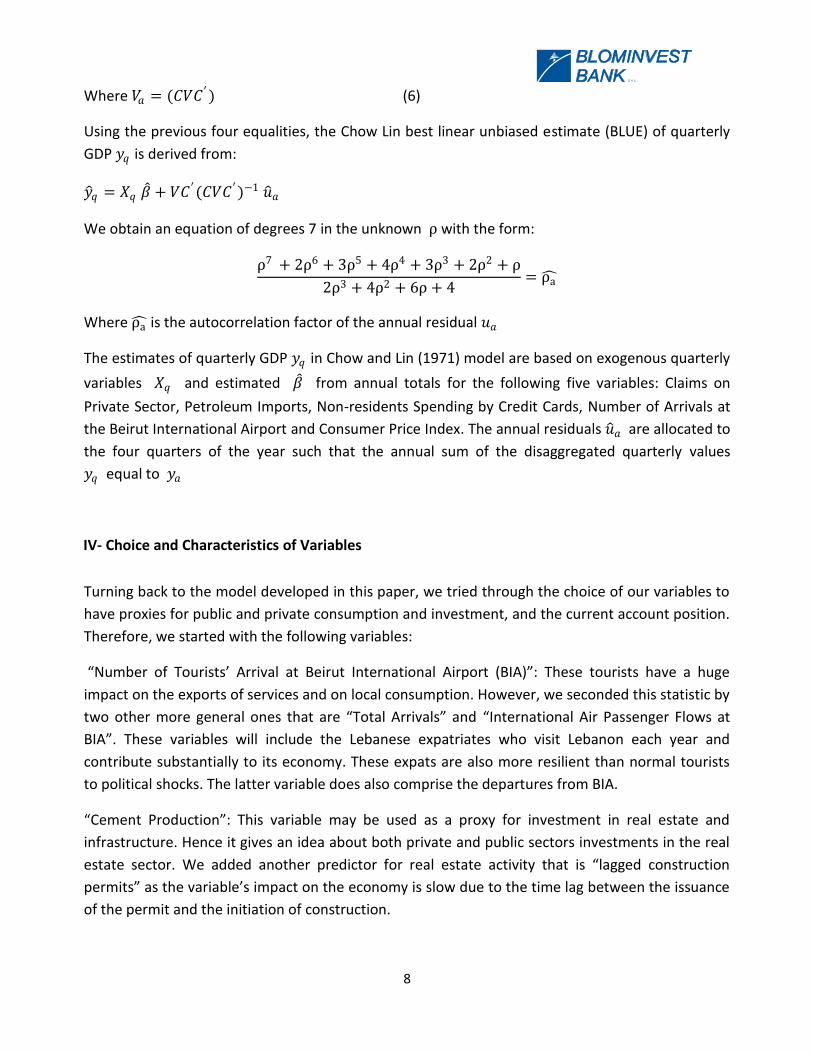
Where 𝑉𝑎 = (𝐶𝑉𝐶′) (6)

Using the previous four equalities, the Chow Lin best linear unbiased estimate (BLUE) of quarterly

GDP 𝑦𝑞 is derived from:

𝑦 𝑞 = 𝑋𝑞 𝛽 + 𝑉𝐶′(𝐶𝑉𝐶′)−1 𝑢 𝑎

We obtain an equation of degrees 7 in the unknown ρ with the form:

ρ7 + 2ρ6 + 3ρ5 + 4ρ4 + 3ρ3 + 2ρ2 + ρ

2ρ3 + 4ρ2 + 6ρ + 4= ρa

Where ρa is the autocorrelation factor of the annual residual 𝑢𝑎

The estimates of quarterly GDP 𝑦𝑞 in Chow and Lin (1971) model are based on exogenous quarterly

variables 𝑋𝑞 and estimated 𝛽 from annual totals for the following five variables: Claims on

Private Sector, Petroleum Imports, Non-residents Spending by Credit Cards, Number of Arrivals at

the Beirut International Airport and Consumer Price Index. The annual residuals 𝑢 𝑎 are allocated to

the four quarters of the year such that the annual sum of the disaggregated quarterly values

𝑦𝑞 equal to 𝑦𝑎

IV- Choice and Characteristics of Variables

Turning back to the model developed in this paper, we tried through the choice of our variables to

have proxies for public and private consumption and investment, and the current account position.

Therefore, we started with the following variables:

“Number of Tourists’ Arrival at Beirut International Airport (BIA)”: These tourists have a huge

impact on the exports of services and on local consumption. However, we seconded this statistic by

two other more general ones that are “Total Arrivals” and “International Air Passenger Flows at

BIA”. These variables will include the Lebanese expatriates who visit Lebanon each year and

contribute substantially to its economy. These expats are also more resilient than normal tourists

to political shocks. The latter variable does also comprise the departures from BIA.

“Cement Production”: This variable may be used as a proxy for investment in real estate and

infrastructure. Hence it gives an idea about both private and public sectors investments in the real

estate sector. We added another predictor for real estate activity that is “lagged construction

permits” as the variable’s impact on the economy is slow due to the time lag between the issuance

of the permit and the initiation of construction.

9

S A L

“Claims on Private Sector”: This variable is used as a proxy private consumption and private

investment as well. Claims on private sector comprise personal and consumption loans contracted

by individuals for their purchases of cars, furniture, daily consumption, etc. The variable also

includes loans allocated to businesses for their expansion purposes and thus will in this regard

represent investment of the private sector.

“Petroleum Imports”: This variable will give an idea about the consumption level and more

generally about the economic activity as an increase in consumption and economic activity will lead

to an increase in the petroleum imports.

“Government Spending”: The considered variable comprises primary spending, thus public debt

service has been excluded. Primary government spending comprises both current spending that

represents public consumption and capital spending that represents public investment.

“Imports of Goods (Excluding Petroleum)” and “exports of goods”: These variables serve as proxies

to measure the external sector contribution to the economy, in addition to the importance of

imports as a proxy to consumption as Lebanon imports more than 80% of its consumption goods.

“Broad Money M3”: This variable represents the impact of monetary policy on the liquidity

available in the market, in addition to the inflow of capital and remittances. So an increase in M3

will most probably have a positive impact on GDP.

“Consumer Price Index”: Besides using the CPI to deflate our nominal variables, we also included

the CPI in our model since high inflation may negatively impact growth, and Lebanon went through

high inflation rates in the 90s. We rebased the CPI to the year 1993 to have a complete time series.

“Cleared Checks”: We thought that the amount or the number of cleared checks will be useful to

represent the general economic activity as the increase in the number and amount of cleared

checks will probably lead to an improvement in the economic activity. This could be used mainly as

another proxy for consumption.

“Non-residents spending by credit cards”: This variable is used as a proxy for the additional exports

of goods and services that are not being taken into account by the exports of goods that are taken

from customs and BDL.

Our sources of data are mainly the websites of the Ministry of Finance and Banque du Liban (BDL).

The figures extracted from the database are available at monthly frequency and so to adjust to

quarterly series, we adopted two different approaches depending on the nature of the indicators: if

the series under construction is that of a flow variable measured over an interval of time, we resort

to adding up the three months figures of each quarter to obtain the quarterly value. If the series

considered relates to a stock variable measured at one specific time, we consider the average value

of the three monthly figures of each quarter as the quarterly value. The approach adopted in the

10

S A L

latter case, allows the derived quarterly figure to capture the changes registered over the course of

the considered quarter.

Before proceeding with the model, we seasonally adjust the real variables, computed by deflating

the nominal variables with the CPI, to remove the noise effects that hide the underlying trend in

real short term changes. The seasonally adjusted series are derived using the Census X-12

algorithm used by the US Bureau of the Census. The procedure consists of decomposing a time

series into three components among which the seasonal component and the irregular component.

We use the multiplicative seasonal adjustment decomposition model to filter the influence of

seasonality, as the magnitude of the seasonal fluctuations vary with the level of the series ( e.g.

number of tourists arrival) which are of positive values.

We apply the Granger Causality test (1969) to determine the endogenous variables for the model.

The test shows whether lagged information on a variable Y provides any statistically significant

information about a variable X in the presence of lagged X. If not, then “Y does not Granger-cause

X”. And so X is said to be exogenous. If “Y Granger cause X” and “X granger cause Y” then X and Y

are said to be endogenous.

The application of the test reduced the number of the endogenous variables of the model to ten

out of fourteen initial variables: GDP, Import Petroleum, Claims on Private Sector, Cement

Production, Total Imports (excluding Petroleum), Arrivals at the Beirut International Airport,

Government Spending, Total Exports, CPI, and Non-resident Spending by Credit Cards.

The remaining four variables are exogenous to the model and include: Money Supply (M3), Lag of

construction permits, cleared checks, and Number of Tourists.

V- The Vector Autoregressive Model (VAR)

The Vector Autoregression (VAR) allows for the forecast of time series and the analysis of dynamic

impact of random disturbances on the system of variables. The VAR approach considers every

endogenous variable as a function of the lagged values of all the endogenous variables in the

system.

We define 𝑌𝑡as:

𝑌𝑡 = 𝑌1𝑡 ,𝑌2𝑡 ,… ,𝑌10𝑡 ′

𝑊𝑕𝑒𝑟𝑒 𝑌𝑖𝑡 , 𝑓𝑜𝑟 𝑖 = 1… 10 𝑎𝑟𝑒 𝑡𝑕𝑒 𝑒𝑛𝑑𝑜𝑔𝑒𝑛𝑜𝑢𝑠 𝑣𝑎𝑟𝑖𝑎𝑏𝑙𝑒𝑠

The VAR (vector autoregressive model) is derived as follow:

11

S A L

𝑌𝑡 = 𝑐 + 𝛷1𝑌𝑡−1 + 𝛷2𝑌𝑡−2 +⋯+ 𝛷𝑝𝑌𝑡−𝑝 + 𝜀𝑡

𝑊𝑕𝑒𝑟𝑒 𝑐 𝑑𝑒𝑛𝑜𝑡𝑒𝑠 𝑎 (10 𝑥 1) 𝑣𝑒𝑐𝑡𝑜𝑟 𝑜𝑓 𝑐𝑜𝑛𝑠𝑡𝑎𝑛𝑡𝑠 𝑐1 , 𝑐2 ,… , 𝑐10

′

𝛷𝑗 = 𝛷11

(𝑗 ) ⋯ 𝛷110(𝑗 )

⋮ ⋱ ⋮

𝛷91(𝑗 ) ⋯ 𝛷910

(𝑗 ) for 𝑗 = 1,2,… , 𝑝

𝐴𝑛𝑑 𝜀𝑡 = (𝜀1𝑡 , 𝜀2𝑡 ,… , 𝜀10𝑡)′ 𝑤𝑖𝑡𝑕

𝐸 𝜀𝑡 = 010×10 𝑎𝑛𝑑

𝐸 𝜀𝑡𝜀𝜏′ =

𝛺 𝑓𝑜𝑟 𝑡 = 𝜏010×10 𝑜𝑡𝑕𝑒𝑟𝑤𝑖𝑠𝑒

𝑊𝑕𝑒𝑟𝑒 𝛺 𝑖𝑠 𝑎 10 × 10 𝑠𝑦𝑚𝑚𝑒𝑡𝑟𝑖𝑐 𝑝𝑜𝑠𝑖𝑡𝑖𝑣𝑒 𝑑𝑒𝑓𝑖𝑛𝑖𝑡𝑒 𝑚𝑎𝑡𝑟𝑖𝑥

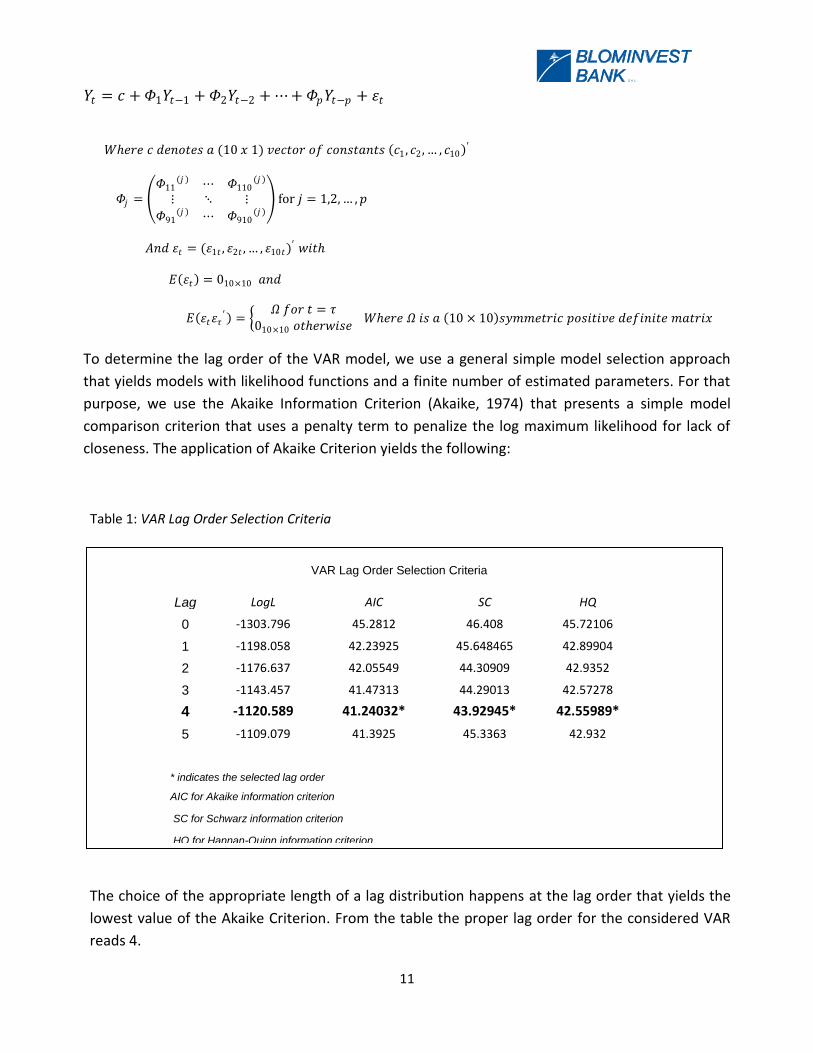
To determine the lag order of the VAR model, we use a general simple model selection approach

that yields models with likelihood functions and a finite number of estimated parameters. For that

purpose, we use the Akaike Information Criterion (Akaike, 1974) that presents a simple model

comparison criterion that uses a penalty term to penalize the log maximum likelihood for lack of

closeness. The application of Akaike Criterion yields the following:

Table 1: VAR Lag Order Selection Criteria

The choice of the appropriate length of a lag distribution happens at the lag order that yields the

lowest value of the Akaike Criterion. From the table the proper lag order for the considered VAR

reads 4.

VAR Lag Order Selection Criteria

Lag LogL AIC SC HQ

0 -1303.796 45.2812 46.408 45.72106

1 -1198.058 42.23925 45.648465 42.89904

2 -1176.637 42.05549 44.30909 42.9352

3 -1143.457 41.47313 44.29013 42.57278

4 -1120.589 41.24032* 43.92945* 42.55989*

5 -1109.079 41.3925 45.3363 42.932

* indicates the selected lag order

AIC for Akaike information criterion

SC for Schwarz information criterion

HQ for Hannan-Quinn information criterion

12

S A L

Alternative general criteria exist for model selection. The most common are the Hannan-Quinn

Criterion (1979) and the Schwartz Criterion (1978). For the considered VAR model, the latter two

methods yield the same outcome as the Akaike Criterion, strengthening the choice of the adopted

model selection. This is expected to a certain extent as a lag order of 4 means that the effect of a

variable change in a specific quarter will impact GDP for the whole year.

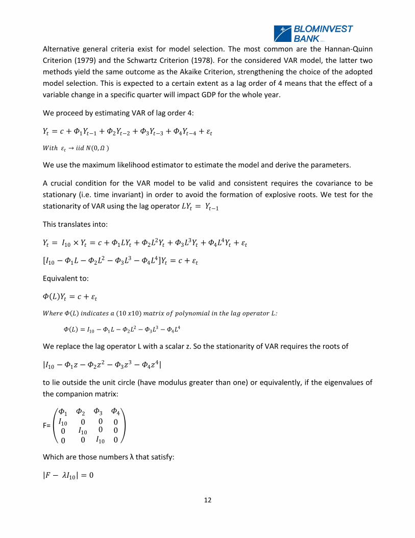
We proceed by estimating VAR of lag order 4:

𝑌𝑡 = 𝑐 + 𝛷1𝑌𝑡−1 + 𝛷2𝑌𝑡−2 + 𝛷3𝑌𝑡−3 + 𝛷4𝑌𝑡−4 + 𝜀𝑡

𝑊𝑖𝑡𝑕 𝜀𝑡 → 𝑖𝑖𝑑 𝑁(0,𝛺 )

We use the maximum likelihood estimator to estimate the model and derive the parameters.

A crucial condition for the VAR model to be valid and consistent requires the covariance to be

stationary (i.e. time invariant) in order to avoid the formation of explosive roots. We test for the

stationarity of VAR using the lag operator 𝐿𝑌𝑡 = 𝑌𝑡−1

This translates into:

𝑌𝑡 = 𝐼10 × 𝑌𝑡 = 𝑐 + 𝛷1𝐿𝑌𝑡 + 𝛷2𝐿2𝑌𝑡 + 𝛷3𝐿

3𝑌𝑡 + 𝛷4𝐿4𝑌𝑡 + 𝜀𝑡

𝐼10 − 𝛷1𝐿 − 𝛷2𝐿2 − 𝛷3𝐿

3 − 𝛷4𝐿4 𝑌𝑡 = 𝑐 + 𝜀𝑡

Equivalent to:

𝛷 𝐿 𝑌𝑡 = 𝑐 + 𝜀𝑡

𝑊𝑕𝑒𝑟𝑒 𝛷 𝐿 𝑖𝑛𝑑𝑖𝑐𝑎𝑡𝑒𝑠 𝑎 (10 𝑥10) 𝑚𝑎𝑡𝑟𝑖𝑥 𝑜𝑓 𝑝𝑜𝑙𝑦𝑛𝑜𝑚𝑖𝑎𝑙 𝑖𝑛 𝑡𝑕𝑒 𝑙𝑎𝑔 𝑜𝑝𝑒𝑟𝑎𝑡𝑜𝑟 𝐿:

𝛷 𝐿 = 𝐼10 − 𝛷1𝐿 − 𝛷2𝐿2 − 𝛷3𝐿

3 − 𝛷4𝐿4

We replace the lag operator L with a scalar z. So the stationarity of VAR requires the roots of

𝐼10 − 𝛷1𝑧 − 𝛷2𝑧2 − 𝛷3𝑧

3 − 𝛷4𝑧4

to lie outside the unit circle (have modulus greater than one) or equivalently, if the eigenvalues of

the companion matrix:

F=

𝛷1 𝛷2 𝛷3 𝛷4

𝐼10

00

0𝐼10

0

00𝐼10

000

Which are those numbers λ that satisfy:

𝐹 − 𝜆𝐼10 = 0

13

S A L

Are less than one.

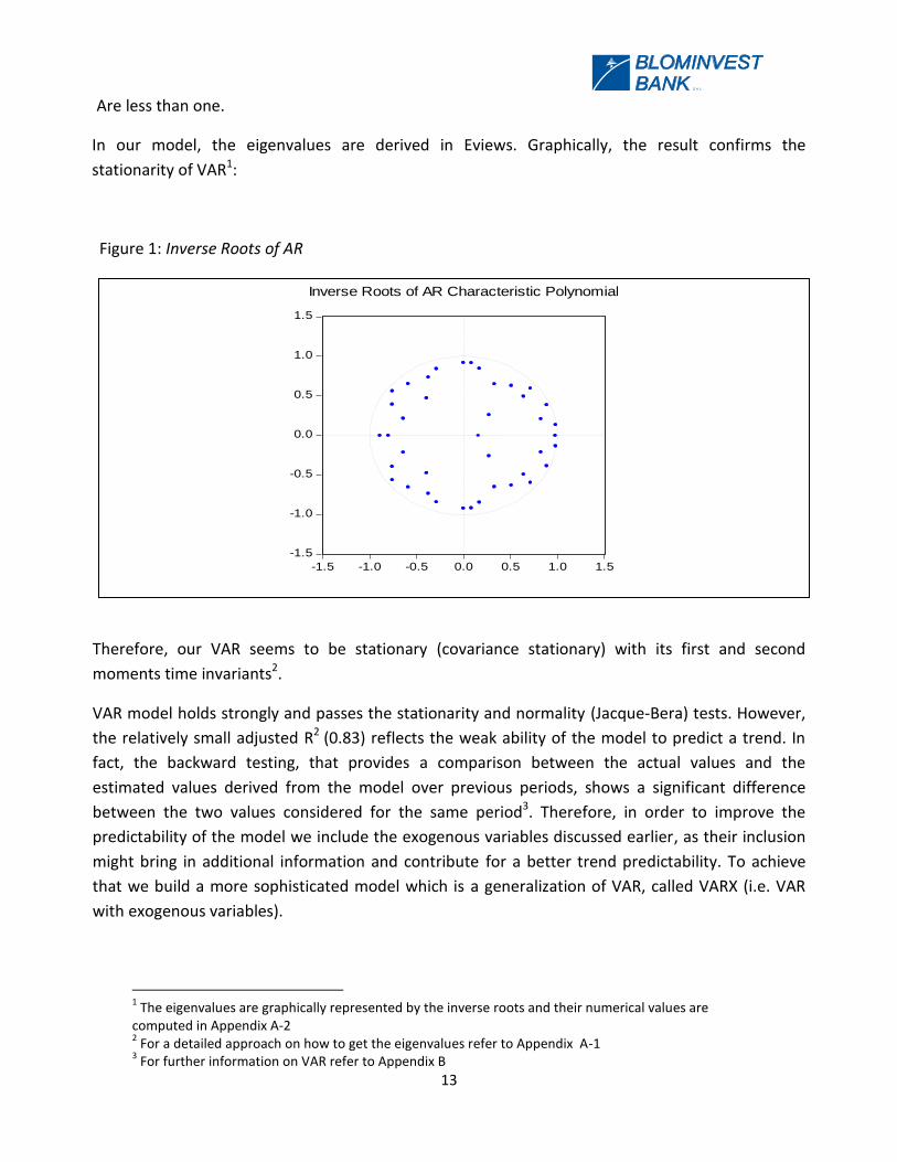
In our model, the eigenvalues are derived in Eviews. Graphically, the result confirms the

stationarity of VAR1:

Figure 1: Inverse Roots of AR

Therefore, our VAR seems to be stationary (covariance stationary) with its first and second

moments time invariants2.

VAR model holds strongly and passes the stationarity and normality (Jacque-Bera) tests. However,

the relatively small adjusted R2 (0.83) reflects the weak ability of the model to predict a trend. In

fact, the backward testing, that provides a comparison between the actual values and the

estimated values derived from the model over previous periods, shows a significant difference

between the two values considered for the same period3. Therefore, in order to improve the

predictability of the model we include the exogenous variables discussed earlier, as their inclusion

might bring in additional information and contribute for a better trend predictability. To achieve

that we build a more sophisticated model which is a generalization of VAR, called VARX (i.e. VAR

with exogenous variables).

1 The eigenvalues are graphically represented by the inverse roots and their numerical values are

computed in Appendix A-2 2 For a detailed approach on how to get the eigenvalues refer to Appendix A-1

3 For further information on VAR refer to Appendix B

-1.5

-1.0

-0.5

0.0

0.5

1.0

1.5

-1.5 -1.0 -0.5 0.0 0.5 1.0 1.5

Inverse Roots of AR Characteristic Polynomial

14

S A L

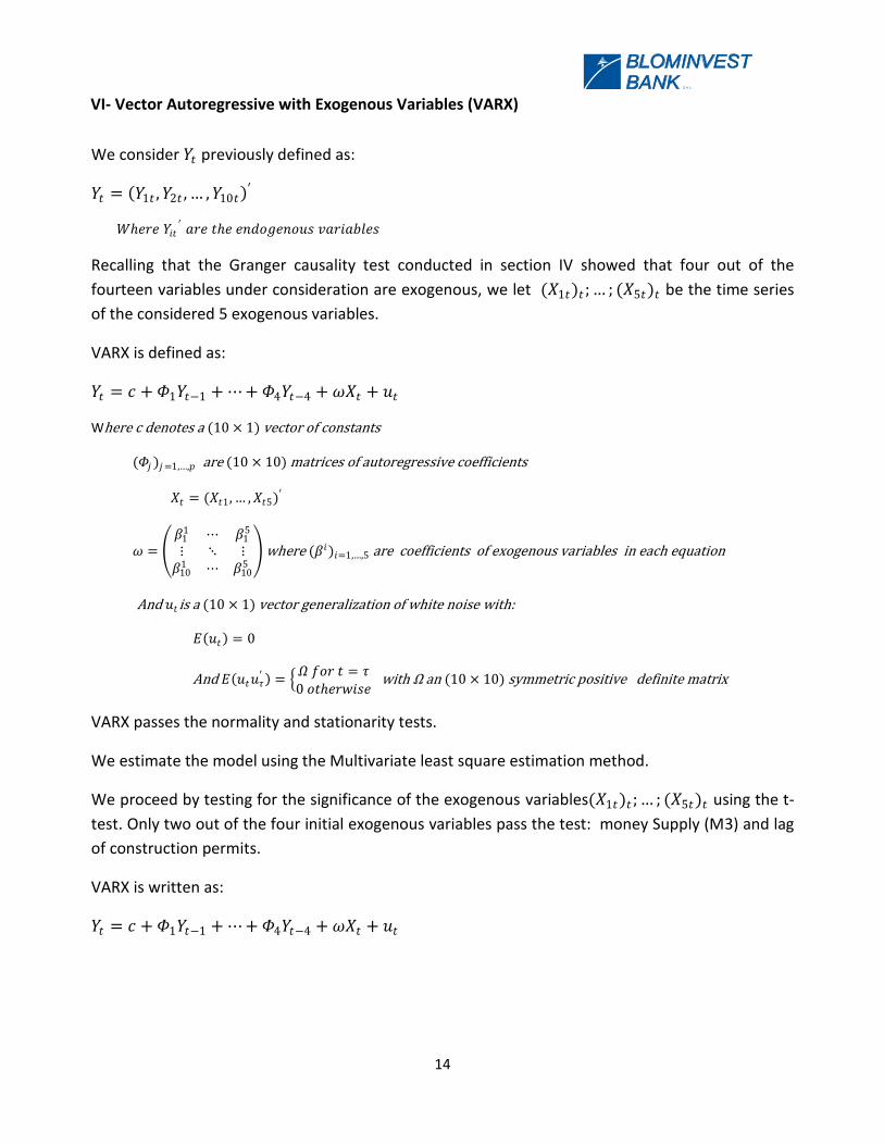
VI- Vector Autoregressive with Exogenous Variables (VARX)

We consider 𝑌𝑡 previously defined as:

𝑌𝑡 = 𝑌1𝑡 ,𝑌2𝑡 ,… ,𝑌10𝑡 ′

𝑊𝑕𝑒𝑟𝑒 𝑌𝑖𝑡′ 𝑎𝑟𝑒 𝑡𝑕𝑒 𝑒𝑛𝑑𝑜𝑔𝑒𝑛𝑜𝑢𝑠 𝑣𝑎𝑟𝑖𝑎𝑏𝑙𝑒𝑠

Recalling that the Granger causality test conducted in section IV showed that four out of the

fourteen variables under consideration are exogenous, we let (𝑋1𝑡)𝑡 ;… ; (𝑋5𝑡)𝑡 be the time series

of the considered 5 exogenous variables.

VARX is defined as:

𝑌𝑡 = 𝑐 + 𝛷1𝑌𝑡−1 +⋯+ 𝛷4𝑌𝑡−4 + 𝜔𝑋𝑡 + 𝑢𝑡

Where c denotes a (10 × 1) vector of constants

(𝛷𝑗 )𝑗=1,…,𝑝 are (10 × 10) matrices of autoregressive coefficients

𝑋𝑡 = (𝑋𝑡1,… ,𝑋𝑡5)′

𝜔 = 𝛽1

1 ⋯ 𝛽15

⋮ ⋱ ⋮𝛽10

1 ⋯ 𝛽105 where (𝛽𝑖)𝑖=1,…,5 are coefficients of exogenous variables in each equation

And 𝑢𝑡 is a (10 × 1) vector generalization of white noise with:

𝐸 𝑢𝑡 = 0

And 𝐸 𝑢𝑡𝑢𝜏′ =

𝛺 𝑓𝑜𝑟 𝑡 = 𝜏0 𝑜𝑡𝑕𝑒𝑟𝑤𝑖𝑠𝑒

with Ω an (10 × 10) symmetric positive definite matrix

VARX passes the normality and stationarity tests.

We estimate the model using the Multivariate least square estimation method.

We proceed by testing for the significance of the exogenous variables(𝑋1𝑡)𝑡 ;… ; (𝑋5𝑡)𝑡 using the t-

test. Only two out of the four initial exogenous variables pass the test: money Supply (M3) and lag

of construction permits.

VARX is written as:

𝑌𝑡 = 𝑐 + 𝛷1𝑌𝑡−1 +⋯+ 𝛷4𝑌𝑡−4 + 𝜔𝑋𝑡 + 𝑢𝑡

15

S A L

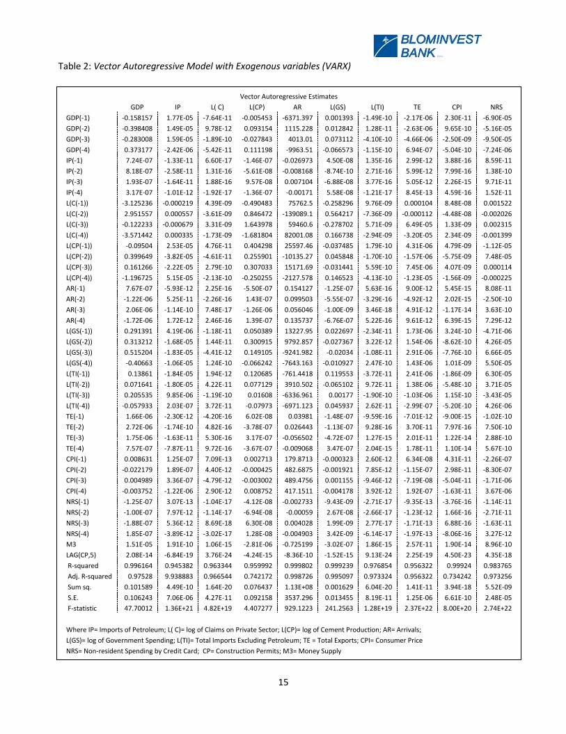
Table 2: Vector Autoregressive Model with Exogenous variables (VARX)

Vector Autoregressive Estimates

GDP IP L( C) L(CP) AR L(GS) L(TI) TE CPI NRS

GDP(-1) -0.158157 1.77E-05 -7.64E-11 -0.005453 -6371.397 0.001393 -1.49E-10 -2.17E-06 2.30E-11 -6.90E-05

GDP(-2) -0.398408 1.49E-05 9.78E-12 0.093154 1115.228 0.012842 1.28E-11 -2.63E-06 9.65E-10 -5.16E-05

GDP(-3) -0.283008 1.59E-05 -1.89E-10 -0.027843 4013.01 0.073112 -4.10E-10 -4.66E-06 -2.50E-09 -9.50E-05

GDP(-4) 0.373177 -2.42E-06 -5.42E-11 0.111198 -9963.51 -0.066573 -1.15E-10 6.94E-07 -5.04E-10 -7.24E-06

IP(-1) 7.24E-07 -1.33E-11 6.60E-17 -1.46E-07 -0.026973 4.50E-08 1.35E-16 2.99E-12 3.88E-16 8.59E-11

IP(-2) 8.18E-07 -2.58E-11 1.31E-16 -5.61E-08 -0.008168 -8.74E-10 2.71E-16 5.99E-12 7.99E-16 1.38E-10

IP(-3) 1.93E-07 -1.64E-11 1.88E-16 9.57E-08 0.007104 -6.88E-08 3.77E-16 5.05E-12 2.26E-15 9.71E-11

IP(-4) 3.17E-07 -1.01E-12 -1.92E-17 -1.36E-07 -0.00171 5.58E-08 -1.21E-17 8.45E-13 4.59E-16 1.52E-11

L(C(-1)) -3.125236 -0.000219 4.39E-09 -0.490483 75762.5 -0.258296 9.76E-09 0.000104 8.48E-08 0.001522

L(C(-2)) 2.951557 0.000557 -3.61E-09 0.846472 -139089.1 0.564217 -7.36E-09 -0.000112 -4.48E-08 -0.002026

L(C(-3)) -0.122233 -0.000679 3.31E-09 1.643978 59460.6 -0.278702 5.71E-09 6.49E-05 1.33E-09 0.002315

L(C(-4)) -3.571442 0.000335 -1.73E-09 -1.681804 82001.08 0.166738 -2.94E-09 -3.20E-05 2.34E-09 -0.001399

L(CP(-1)) -0.09504 2.53E-05 4.76E-11 0.404298 25597.46 -0.037485 1.79E-10 4.31E-06 4.79E-09 -1.12E-05

L(CP(-2)) 0.399649 -3.82E-05 -4.61E-11 0.255901 -10135.27 0.045848 -1.70E-10 -1.57E-06 -5.75E-09 7.48E-05

L(CP(-3)) 0.161266 -2.22E-05 2.79E-10 0.307033 15171.69 -0.031441 5.59E-10 7.45E-06 4.07E-09 0.000114

L(CP(-4)) -1.196725 5.15E-05 -2.13E-10 -0.250255 -2127.578 0.146523 -4.13E-10 -1.23E-05 -1.56E-09 -0.000225

AR(-1) 7.67E-07 -5.93E-12 2.25E-16 -5.50E-07 0.154127 -1.25E-07 5.63E-16 9.00E-12 5.45E-15 8.08E-11

AR(-2) -1.22E-06 5.25E-11 -2.26E-16 1.43E-07 0.099503 -5.55E-07 -3.29E-16 -4.92E-12 2.02E-15 -2.50E-10

AR(-3) 2.06E-06 -1.14E-10 7.48E-17 -1.26E-06 0.056046 -1.00E-09 3.46E-18 4.91E-12 -1.17E-14 3.63E-10

AR(-4) -1.72E-06 1.72E-12 2.46E-16 1.39E-07 0.135737 -6.76E-07 5.22E-16 9.61E-12 6.39E-15 7.29E-12

L(GS(-1)) 0.291391 4.19E-06 -1.18E-11 0.050389 13227.95 0.022697 -2.34E-11 1.73E-06 3.24E-10 -4.71E-06

L(GS(-2)) 0.313212 -1.68E-05 1.44E-11 0.300915 9792.857 -0.027367 3.22E-12 1.54E-06 -8.62E-10 4.26E-05

L(GS(-3)) 0.515204 -1.83E-05 -4.41E-12 0.149105 -9241.982 -0.02034 -1.08E-11 2.91E-06 -7.76E-10 6.66E-05

L(GS(-4)) -0.40663 -1.06E-05 1.24E-10 -0.066242 -7643.163 -0.010927 2.47E-10 1.43E-06 1.01E-09 5.50E-05

L(TI(-1)) 0.13861 -1.84E-05 1.94E-12 0.120685 -761.4418 0.119553 -3.72E-11 2.41E-06 -1.86E-09 6.30E-05

L(TI(-2)) 0.071641 -1.80E-05 4.22E-11 0.077129 3910.502 -0.065102 9.72E-11 1.38E-06 -5.48E-10 3.71E-05

L(TI(-3)) 0.205535 9.85E-06 -1.19E-10 0.01608 -6336.961 0.00177 -1.90E-10 -1.03E-06 1.15E-10 -3.43E-05

L(TI(-4)) -0.057933 2.03E-07 3.72E-11 -0.07973 -6971.123 0.045937 2.62E-11 -2.99E-07 -5.20E-10 4.26E-06

TE(-1) 1.66E-06 -2.30E-12 -4.20E-16 6.02E-08 0.03981 -1.48E-07 -9.59E-16 -7.01E-12 -9.00E-15 -1.02E-10

TE(-2) 2.72E-06 -1.74E-10 4.82E-16 -3.78E-07 0.026443 -1.13E-07 9.28E-16 3.70E-11 7.97E-16 7.50E-10

TE(-3) 1.75E-06 -1.63E-11 5.30E-16 3.17E-07 -0.056502 -4.72E-07 1.27E-15 2.01E-11 1.22E-14 2.88E-10

TE(-4) 7.57E-07 -7.87E-11 9.72E-16 -3.67E-07 -0.009068 3.47E-07 2.04E-15 1.78E-11 1.10E-14 5.67E-10

CPI(-1) 0.008631 1.25E-07 7.09E-13 0.002713 179.8713 -0.000323 2.60E-12 6.34E-08 4.31E-11 -2.26E-07

CPI(-2) -0.022179 1.89E-07 4.40E-12 -0.000425 482.6875 -0.001921 7.85E-12 -1.15E-07 2.98E-11 -8.30E-07

CPI(-3) 0.004989 3.36E-07 -4.79E-12 -0.003002 489.4756 0.001155 -9.46E-12 -7.19E-08 -5.04E-11 -1.71E-06

CPI(-4) -0.003752 -1.22E-06 2.90E-12 0.008752 417.1511 -0.004178 3.92E-12 1.92E-07 -1.63E-11 3.67E-06

NRS(-1) -1.25E-07 3.07E-13 -1.04E-17 -4.12E-08 -0.002733 -9.43E-09 -2.71E-17 -9.35E-13 -3.76E-16 -1.14E-11

NRS(-2) -1.00E-07 7.97E-12 -1.14E-17 -6.94E-08 -0.00059 2.67E-08 -2.66E-17 -1.23E-12 1.66E-16 -2.71E-11

NRS(-3) -1.88E-07 5.36E-12 8.69E-18 6.30E-08 0.004028 1.99E-09 2.77E-17 -1.71E-13 6.88E-16 -1.63E-11

NRS(-4) 1.85E-07 -3.89E-12 -3.02E-17 1.28E-08 -0.004903 3.42E-09 -6.14E-17 -1.97E-13 -8.06E-16 3.27E-12

M3 1.51E-05 1.91E-10 1.06E-15 -2.81E-06 -0.725199 -3.02E-07 1.86E-15 2.57E-11 1.90E-14 8.96E-10

LAG(CP,5) 2.08E-14 -6.84E-19 3.76E-24 -4.24E-15 -8.36E-10 -1.52E-15 9.13E-24 2.25E-19 4.50E-23 4.35E-18

R-squared 0.996164 0.945382 0.963344 0.959992 0.999802 0.999239 0.976854 0.956322 0.99924 0.983765

Adj. R-squared 0.97528 9.938883 0.966544 0.742172 0.998726 0.995097 0.973324 0.956322 0.734242 0.973256

Sum sq. 0.101589 4.49E-10 1.64E-20 0.076437 1.13E+08 0.001629 6.04E-20 1.41E-11 3.94E-18 5.52E-09

S.E. 0.106243 7.06E-06 4.27E-11 0.092158 3537.296 0.013455 8.19E-11 1.25E-06 6.61E-10 2.48E-05

F-statistic 47.70012 1.36E+21 4.82E+19 4.407277 929.1223 241.2563 1.28E+19 2.37E+22 8.00E+20 2.74E+22

Where IP= Imports of Petroleum; L( C)= log of Claims on Private Sector; L(CP)= log of Cement Production; AR= Arrivals;

L(GS)= log of Government Spending; L(TI)= Total Imports Excluding Petroleum; TE = Total Exports; CPI= Consumer Price

NRS= Non-resident Spending by Credit Card; CP= Construction Permits; M3= Money Supply

16

S A L

Some of the coefficients’ signs may be unexpected. However, it shows in the impulse response

function that for example, any change in claims on the private sector during a specific quarter will

lead to an increase of GDP over the upcoming year eventhough LC (-1) and LC(-4) have negative

coefficients. The results of the model as a whole were very satisfactory as at shows.

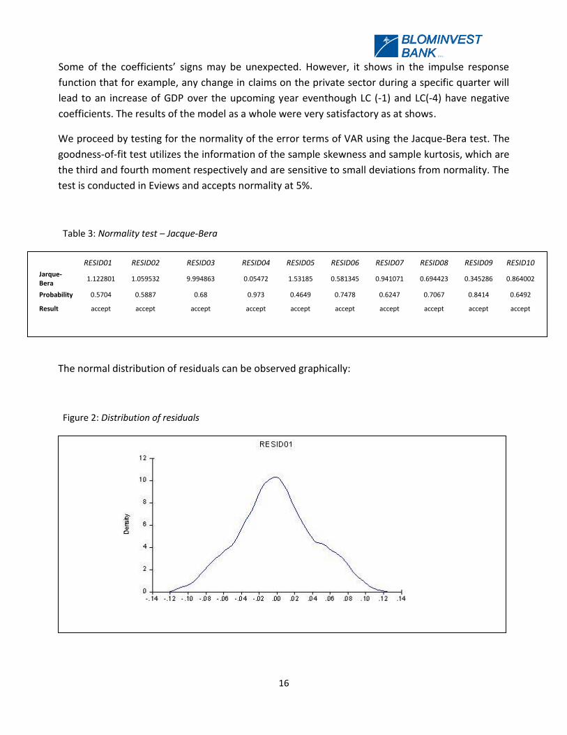
We proceed by testing for the normality of the error terms of VAR using the Jacque-Bera test. The

goodness-of-fit test utilizes the information of the sample skewness and sample kurtosis, which are

the third and fourth moment respectively and are sensitive to small deviations from normality. The

test is conducted in Eviews and accepts normality at 5%.

Table 3: Normality test – Jacque-Bera

The normal distribution of residuals can be observed graphically:

Figure 2: Distribution of residuals

RESID01 RESID02 RESID03 RESID04 RESID05 RESID06 RESID07 RESID08 RESID09 RESID10

Jarque-Bera

1.122801 1.059532 9.994863 0.05472 1.53185 0.581345 0.941071 0.694423 0.345286 0.864002

Probability 0.5704 0.5887 0.68 0.973 0.4649 0.7478 0.6247 0.7067 0.8414 0.6492

Result accept accept accept accept accept accept accept accept accept accept

17

S A L

We have assumed throughout the model residual means of zero. We use the empirical distribution

test to prove it. The test, applied to each residual term of a normal series, provides the mean and

the standard error of each series and test the significance of each one. Here follows the result of

the test applied to the residual term of GDP:

Table 4: Empirical Distribution Test

The application of the test to the remaining nine residual terms reveals that the all ten variables are

all normally distributed with mean zero.

We proceed by testing for the serial correlation of residuals. We apply the Durbin Watson statistic

test that yields a value of 2.085, showing that residuals are independent over time.

VARX is proved to be consistent and significant with normal independent residuals of zero mean.

The model holds strongly with a high adjusted R2 of 97.5%. The backward testing shows a

significant similarity between the series generated by the estimated model and the actual data.

This strengthens the performance of the model and its ability to predict future trends.

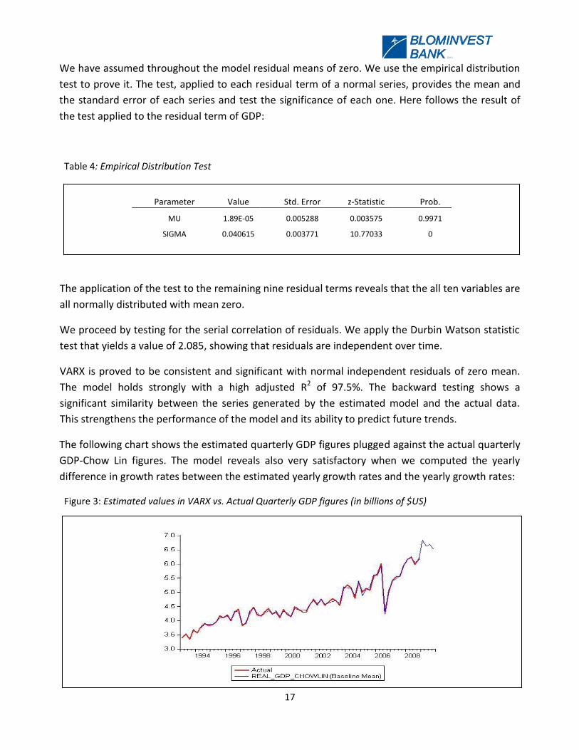
The following chart shows the estimated quarterly GDP figures plugged against the actual quarterly

GDP-Chow Lin figures. The model reveals also very satisfactory when we computed the yearly

difference in growth rates between the estimated yearly growth rates and the yearly growth rates:

Figure 3: Estimated values in VARX vs. Actual Quarterly GDP figures (in billions of $US)

Parameter Value Std. Error z-Statistic Prob.

MU 1.89E-05 0.005288 0.003575 0.9971

SIGMA 0.040615 0.003771 10.77033 0

18

S A L

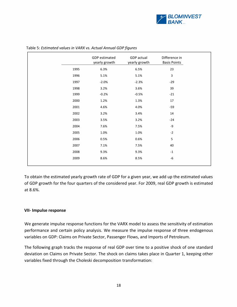
Table 5: Estimated values in VARX vs. Actual Annual GDP figures

GDP estimated yearly growth

GDP actual yearly growth

Difference in Basis Points

1995 6.3% 6.5% 23

1996 5.1% 5.1% 3

1997 -2.0% -2.3% -29

1998 3.2% 3.6% 39

1999 -0.2% -0.5% -21

2000 1.2% 1.3% 17

2001 4.6% 4.0% -59

2002 3.2% 3.4% 14

2003 3.5% 3.2% -24

2004 7.6% 7.5% -9

2005 1.0% 1.0% -2

2006 0.5% 0.6% 5

2007 7.1% 7.5% 40

2008 9.3% 9.3% -1

2009 8.6% 8.5% -6

To obtain the estimated yearly growth rate of GDP for a given year, we add up the estimated values

of GDP growth for the four quarters of the considered year. For 2009, real GDP growth is estimated

at 8.6%.

VII- Impulse response

We generate impulse response functions for the VARX model to assess the sensitivity of estimation

performance and certain policy analysis. We measure the impulse response of three endogenous

variables on GDP: Claims on Private Sector, Passenger Flows, and Imports of Petroleum.

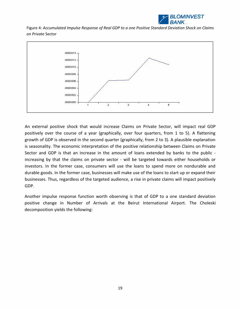
The following graph tracks the response of real GDP over time to a positive shock of one standard

deviation on Claims on Private Sector. The shock on claims takes place in Quarter 1, keeping other

variables fixed through the Choleski decomposition transformation:

19

S A L

Figure 4: Accumulated Impulse Response of Real GDP to a one Positive Standard Deviation Shock on Claims

on Private Sector

An external positive shock that would increase Claims on Private Sector, will impact real GDP

positively over the course of a year (graphically, over four quarters, from 1 to 5). A flattening

growth of GDP is observed in the second quarter (graphically, from 2 to 3). A plausible explanation

is seasonality. The economic interpretation of the positive relationship between Claims on Private

Sector and GDP is that an increase in the amount of loans extended by banks to the public -

increasing by that the claims on private sector - will be targeted towards either households or

investors. In the former case, consumers will use the loans to spend more on nondurable and

durable goods. In the former case, businesses will make use of the loans to start up or expand their

businesses. Thus, regardless of the targeted audience, a rise in private claims will impact positively

GDP.

Another impulse response function worth observing is that of GDP to a one standard deviation

positive change in Number of Arrivals at the Beirut International Airport. The Choleski

decomposition yields the following:

20

S A L

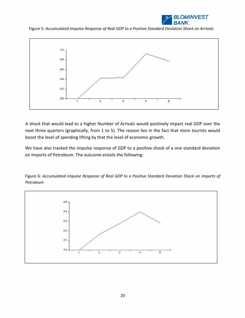
Figure 5: Accumulated Impulse Response of Real GDP to a Positive Standard Deviation Shock on Arrivals

A shock that would lead to a higher Number of Arrivals would positively impact real GDP over the

next three quarters (graphically, from 1 to 5). The reason lies in the fact that more tourists would

boost the level of spending lifting by that the level of economic growth.

We have also tracked the impulse response of GDP to a positive shock of a one standard deviation

on Imports of Petroleum. The outcome entails the following:

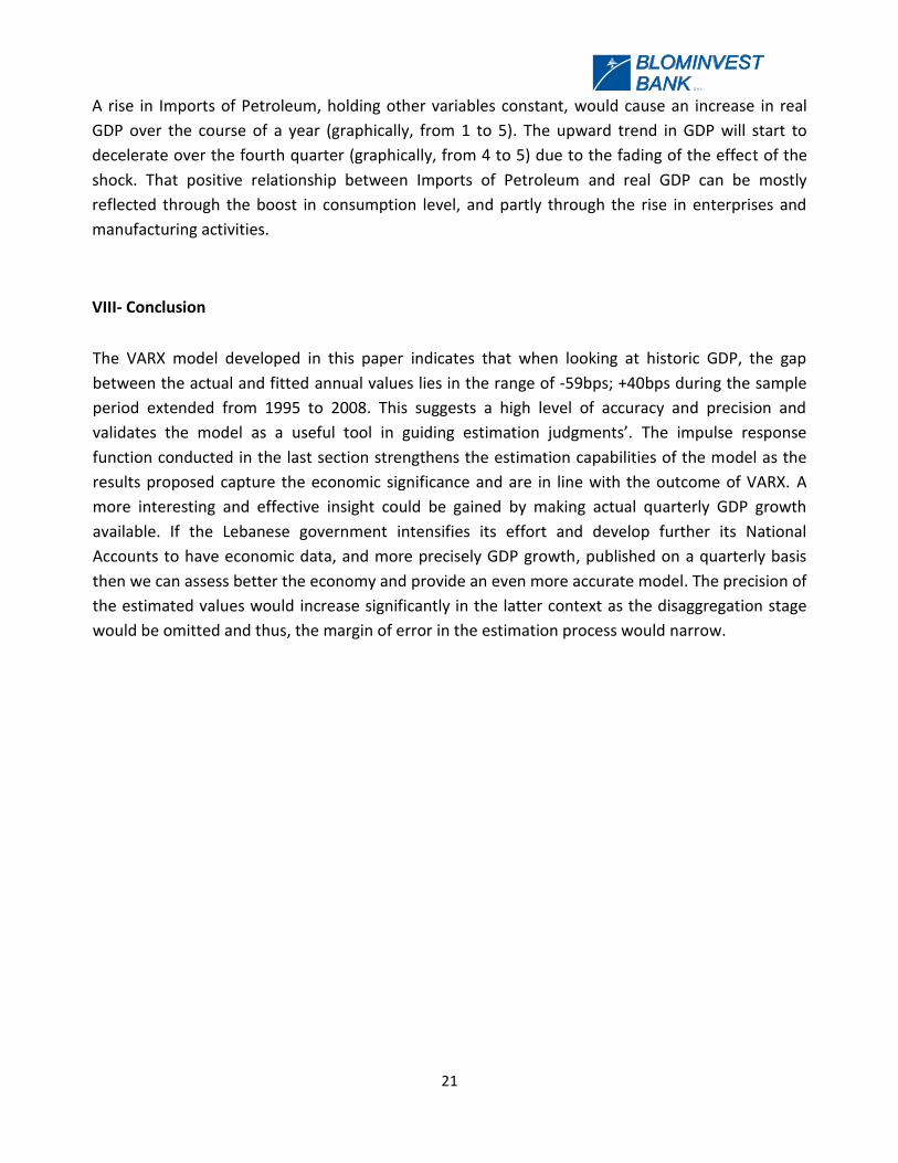
Figure 6: Accumulated Impulse Response of Real GDP to a Positive Standard Deviation Shock on Imports of

Petroleum

21

S A L

A rise in Imports of Petroleum, holding other variables constant, would cause an increase in real

GDP over the course of a year (graphically, from 1 to 5). The upward trend in GDP will start to

decelerate over the fourth quarter (graphically, from 4 to 5) due to the fading of the effect of the

shock. That positive relationship between Imports of Petroleum and real GDP can be mostly

reflected through the boost in consumption level, and partly through the rise in enterprises and

manufacturing activities.

VIII- Conclusion

The VARX model developed in this paper indicates that when looking at historic GDP, the gap

between the actual and fitted annual values lies in the range of -59bps; +40bps during the sample

period extended from 1995 to 2008. This suggests a high level of accuracy and precision and

validates the model as a useful tool in guiding estimation judgments’. The impulse response

function conducted in the last section strengthens the estimation capabilities of the model as the

results proposed capture the economic significance and are in line with the outcome of VARX. A

more interesting and effective insight could be gained by making actual quarterly GDP growth

available. If the Lebanese government intensifies its effort and develop further its National

Accounts to have economic data, and more precisely GDP growth, published on a quarterly basis

then we can assess better the economy and provide an even more accurate model. The precision of

the estimated values would increase significantly in the latter context as the disaggregation stage

would be omitted and thus, the margin of error in the estimation process would narrow.

22

S A L

References

Bell, W. R., Chen, B. C., Findley, D. F., Monsell, B.C. and Otto, M. C. (1998), “New Capabilities and Methods of

the Census X-12 Seasonal Adjustment Programs”, Journal of Business and Economic Statistics, 16, 2, 127-

176.

Bera, A. K. and Jarque, C. M. (1987), “A Test for Normality of Observations and Regression Residuals” ,

International Statistical Review,55, 2, 163-172.

Bruggemann, R. and Lutkepohl, H. (2000), “Lag Selection in Subset VAR Models with an Application to a US

Monetary System”, Institute for Statistics and Econometrics.

Caro, A. R., Feijoo, S. R. and Quintana, D. D. (2003), “Methods for Quarterly Disaggregation Without

Indicators; a Comparative Study Using Simulation”, Computational Statistics and Data Analysis, 43, 1, 63-78.

Carriero, A., Marcellino, M. and Kapetanius, G. (2010) “Forecasting large datasets with Reduced Rank

Multivariate Models”, European University Institute.

Chen, B. (2007), “An Emperical Comparison of Methods for Temporal Disaggregation at the National

Account”, Bureau of Economic Analysis.

Chow, G and Lin, A. (1971), “Best Linear Unbiased Interpolation, Distribution, and Extrapolation of Time

Series by Related Series”, The Review of Economics and Statistics, 53, 4, 372-375.

Fernandez, R. (1981), “A Metohdological Note on the Estimation of Time Series”, The Review of Economics

and Statistics, 63, 471-478.

Fraumeni, B. M., Landefeld, J.S. and Seskin, E.P. (2008), “Taking the Pulse of the Economy: Measuring GDP”,

Journal of Economic Perspectives, 22, 2, 198-216.

Guerrero, V. M. and Martinez, I. (1995), “A recursive ARIMA-based Procedure for Disaggregating a Time

Series Variable using Concurrent Data”, Test, 4, 2, 359-379.

Hamilton, J. D. (1994), “Time Series Analysis” Princeton Universtiy Press.

Hedhili, L. and Trabelsi, A. (2005), “A Polynomial Moethod for Temporal Disaggregation of Multivariate Time

Series”, European Commission.

Luetkepohl, H. (2005), “New Introduction to Multiple Time Series Analysis”, Springer-Verlag Press.

Luetkepohl, H. (2007), “Econometric Analysis with Vector Autoregressive Models”, European University

Institute.

23

S A L

Mitchell, J., Smith, R. J., Weale, M. R., Wright, S and Salazar, L. (2004), “An Indicator of Monthly GDP and an

Early Estimate of Qaurterly GDP Growth”, National Institute of Economic and Social Research, Dsicussino

Paper 127.

Ozcicek, O. (1999), “Lag Length Selection in Vector Autoregressive Models: Symmetric and Assymetric Lags”,

Applied Economics, 31, 4, 517-524.

Proeitti, T. (2006), “Temporal Disaggregation by State Space Methods: Dynamics Regression Metohds

Revised”, The Econometrics Journal, 9, 3, 357-372.

24

S A L

Appendix A - VAR Stationarity

1- Conditions for stationarity

The value of the scalar system of VAR (4) at time t is given by the following dynamic equation:

𝑌𝑡 = 𝑐 + 𝛷1𝑌𝑡−1 + 𝛷2𝑌𝑡−2 + 𝛷3𝑌𝑡−3 + 𝛷4𝑌𝑡−4 + 𝜀𝑡

For our purpose it is more convenient to rewrite 𝑌𝑡 as a first order difference equation in a

vector 𝜉𝑡 . Define:

Vector 𝜉𝑡 by 𝜉𝑡 =

𝑌𝑡𝑌𝑡−1𝑌𝑡−2𝑌𝑡−3

Matrix 𝐹 for a 4th

order by 𝐹 =

𝛷1 𝛷2

𝐼10 0 𝛷3 𝛷4

0 00 𝐼10

0 0

0 0 𝐼10 0

𝐴𝑛𝑑

Vector 𝑉𝑡 by 𝑉𝑡 =

𝜀𝑡000

Under the above notation, consider the following first order difference equation which defines VAR

(4):

𝜉𝑡 = 𝐹𝜉𝑡−1 + 𝑉𝑡

𝑊𝑕𝑒𝑟𝑒 𝐸 𝑉𝑡𝑉𝜏′ =

𝑄 𝑓𝑜𝑟 𝑡 = 𝜏.040×40 𝑜𝑡𝑕𝑒𝑟𝑤𝑖𝑠𝑒.

𝐴𝑛𝑑 𝑄(40×40) = 𝛺 ⋯ 0⋮ ⋱ ⋮0 ⋯ 0

𝛺 𝑏𝑒𝑖𝑛𝑔 𝑡𝑕𝑒 𝑣𝑎𝑟𝑖𝑎𝑛𝑐𝑒 𝑐𝑜𝑣𝑎𝑟𝑖𝑎𝑛𝑐𝑒 𝑚𝑎𝑡𝑟𝑖𝑥 𝑜𝑓 𝜀𝑡

The effect of 𝑌𝑡+𝑗 of a one unit increase in 𝜀𝑡 indicates whether VAR(4) is explosive or stationary: If

the dynamic multiplier is between 0 and 1, then the absolute value of the effect decays

geometrically towards zero and stationarity is satisfied. However, if the dynamic multiplier is lower

or higher than 1, then the system would either exhibit explosive oscillation or the dynamic

multiplier would increase explosively over time.

25

S A L

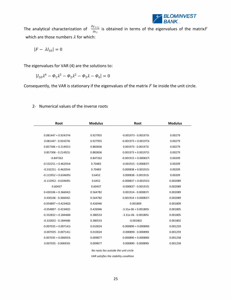
The analytical characterization of 𝜕𝑦 𝑡+𝑗

𝜕𝜀 𝑡 is obtained in terms of the eigenvalues of the matrix𝐹

which are those numbers 𝜆 for which:

𝐹 − 𝜆𝐼10 = 0

The eigenvalues for VAR (4) are the solutions to:

𝐼10𝜆4 − 𝛷1𝜆

3 − 𝛷2𝜆2 − 𝛷3𝜆 − 𝛷4 = 0

Consequently, the VAR is stationary if the eigenvalues of the matrix 𝐹 lie inside the unit circle.

2- Numerical values of the inverse roots

Root Modulus Root Modulus

0.081447 + 0.924374i 0.927955 -0.001973 - 0.001973i 0.00279

0.081447 - 0.924374i 0.927955 -0.001973 + 0.001973i 0.00279

0.857306 + 0.214921i 0.883836 0.001973 - 0.001972i 0.00279

0.857306 - 0.214921i 0.883836 0.001973 + 0.001972i 0.00279

-0.847262 0.847262 -0.001915 + 0.000837i 0.00209

-0.532251 + 0.462054i 0.70483 -0.001915 - 0.000837i 0.00209

-0.532251 - 0.462054i 0.70483 0.000838 + 0.001915i 0.00209

-0.115952 + 0.634695i 0.6452 0.000838 - 0.001915i 0.00209

-0.115952 - 0.634695i 0.6452 -0.000837 + 0.001915i 0.002089

0.60437 0.60437 -0.000837 - 0.001915i 0.002089

0.430106 + 0.366042i 0.564782 0.001914 - 0.000837i 0.002089

0.430106 - 0.366042i 0.564782 0.001914 + 0.000837i 0.002089

-0.054897 + 0.423402i 0.426946 0.001809 0.001809

-0.054897 - 0.423402i 0.426946 -3.31e-06 + 0.001805i 0.001805

-0.332832 + 0.184468i 0.380533 -3.31e-06 - 0.001805i 0.001805

-0.332832 - 0.184468i 0.380533 -0.001802 0.001802

-0.007035 + 0.007141i 0.010024 -0.000890 + 0.000890i 0.001259

-0.007035 - 0.007141i 0.010024 -0.000890 - 0.000890i 0.001259

0.007035 + 0.006933i 0.009877 0.000890 + 0.000890i 0.001258

0.007035 - 0.006933i 0.009877 0.000890 - 0.000890i 0.001258

No roots lies outside the unit circle

VAR satisfies the stability condition

26

S A L

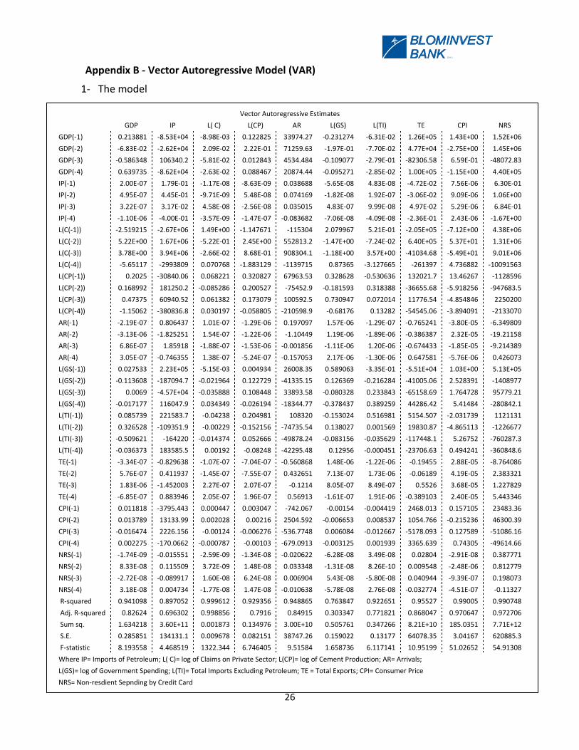
Appendix B - Vector Autoregressive Model (VAR)

1- The model

Vector Autoregressive Estimates

GDP IP L( C) L(CP) AR L(GS) L(TI) TE CPI NRS

GDP(-1) 0.213881 -8.53E+04 -8.98E-03 0.122825 33974.27 -0.231274 -6.31E-02 1.26E+05 1.43E+00 1.52E+06

GDP(-2) -6.83E-02 -2.62E+04 2.09E-02 2.22E-01 71259.63 -1.97E-01 -7.70E-02 4.77E+04 -2.75E+00 1.45E+06

GDP(-3) -0.586348 106340.2 -5.81E-02 0.012843 4534.484 -0.109077 -2.79E-01 -82306.58 6.59E-01 -48072.83

GDP(-4) 0.639735 -8.62E+04 -2.63E-02 0.088467 20874.44 -0.095271 -2.85E-02 1.00E+05 -1.15E+00 4.40E+05

IP(-1) 2.00E-07 1.79E-01 -1.17E-08 -8.63E-09 0.038688 -5.65E-08 4.83E-08 -4.72E-02 7.56E-06 6.30E-01

IP(-2) 4.95E-07 4.45E-01 -9.71E-09 5.48E-08 0.074169 -1.82E-08 1.92E-07 -3.06E-02 9.09E-06 1.06E+00

IP(-3) 3.22E-07 3.17E-02 4.58E-08 -2.56E-08 0.035015 4.83E-07 9.99E-08 4.97E-02 5.29E-06 6.84E-01

IP(-4) -1.10E-06 -4.00E-01 -3.57E-09 -1.47E-07 -0.083682 -7.06E-08 -4.09E-08 -2.36E-01 2.43E-06 -1.67E+00

L(C(-1)) -2.519215 -2.67E+06 1.49E+00 -1.147671 -115304 2.079967 5.21E-01 -2.05E+05 -7.12E+00 4.38E+06

L(C(-2)) 5.22E+00 1.67E+06 -5.22E-01 2.45E+00 552813.2 -1.47E+00 -7.24E-02 6.40E+05 5.37E+01 1.31E+06

L(C(-3)) 3.78E+00 3.94E+06 -2.66E-02 8.68E-01 908304.1 -1.18E+00 3.57E+00 -41034.68 -5.49E+01 9.01E+06

L(C(-4)) -5.65117 -2993809 0.070768 -1.883129 -1139715 0.87365 -3.127665 -261397 4.736882 -10091563

L(CP(-1)) 0.2025 -30840.06 0.068221 0.320827 67963.53 0.328628 -0.530636 132021.7 13.46267 -1128596

L(CP(-2)) 0.168992 181250.2 -0.085286 0.200527 -75452.9 -0.181593 0.318388 -36655.68 -5.918256 -947683.5

L(CP(-3)) 0.47375 60940.52 0.061382 0.173079 100592.5 0.730947 0.072014 11776.54 -4.854846 2250200

L(CP(-4)) -1.15062 -380836.8 0.030197 -0.058805 -210598.9 -0.68176 0.13282 -54545.06 -3.894091 -2133070

AR(-1) -2.19E-07 0.806437 1.01E-07 -1.29E-06 0.197097 1.57E-06 -1.29E-07 -0.765241 -3.80E-05 -6.349809

AR(-2) -3.13E-06 -1.825251 1.54E-07 -1.22E-06 -1.10449 1.19E-06 -1.89E-06 -0.386387 2.32E-05 -19.21158

AR(-3) 6.86E-07 1.85918 -1.88E-07 -1.53E-06 -0.001856 -1.11E-06 1.20E-06 -0.674433 -1.85E-05 -9.214389

AR(-4) 3.05E-07 -0.746355 1.38E-07 -5.24E-07 -0.157053 2.17E-06 -1.30E-06 0.647581 -5.76E-06 0.426073

L(GS(-1)) 0.027533 2.23E+05 -5.15E-03 0.004934 26008.35 0.589063 -3.35E-01 -5.51E+04 1.03E+00 5.13E+05

L(GS(-2)) -0.113608 -187094.7 -0.021964 0.122729 -41335.15 0.126369 -0.216284 -41005.06 2.528391 -1408977

L(GS(-3)) 0.0069 -4.57E+04 -0.035888 0.108448 33893.58 -0.080328 0.233843 -65158.69 1.764728 95779.21

L(GS(-4)) -0.017177 116047.9 0.034349 -0.026194 -18344.77 -0.378437 0.389259 44286.42 5.41484 -280842.1

L(TI(-1)) 0.085739 221583.7 -0.04238 0.204981 108320 -0.153024 0.516981 5154.507 -2.031739 1121131

L(TI(-2)) 0.326528 -109351.9 -0.00229 -0.152156 -74735.54 0.138027 0.001569 19830.87 -4.865113 -1226677

L(TI(-3)) -0.509621 -164220 -0.014374 0.052666 -49878.24 -0.083156 -0.035629 -117448.1 5.26752 -760287.3

L(TI(-4)) -0.036373 183585.5 0.00192 -0.08248 -42295.48 0.12956 -0.000451 -23706.63 0.494241 -360848.6

TE(-1) -3.34E-07 -0.829638 -1.07E-07 -7.04E-07 -0.560868 1.48E-06 -1.22E-06 -0.19455 2.88E-05 -8.764086

TE(-2) 5.76E-07 0.411937 -1.45E-07 -7.55E-07 0.432651 7.13E-07 1.73E-06 -0.06189 4.19E-05 2.383321

TE(-3) 1.83E-06 -1.452003 2.27E-07 2.07E-07 -0.1214 8.05E-07 8.49E-07 0.5526 3.68E-05 1.227829

TE(-4) -6.85E-07 0.883946 2.05E-07 1.96E-07 0.56913 -1.61E-07 1.91E-06 -0.389103 2.40E-05 5.443346

CPI(-1) 0.011818 -3795.443 0.000447 0.003047 -742.067 -0.00154 -0.004419 2468.013 0.157105 23483.36

CPI(-2) 0.013789 13133.99 0.002028 0.00216 2504.592 -0.006653 0.008537 1054.766 -0.215236 46300.39

CPI(-3) -0.016474 2226.156 -0.00124 -0.006276 -536.7748 0.006084 -0.012667 -5178.093 0.127589 -51086.16

CPI(-4) 0.002275 -170.0662 -0.000787 -0.00103 -679.0913 -0.003125 0.001939 3365.639 0.74305 -49614.66

NRS(-1) -1.74E-09 -0.015551 -2.59E-09 -1.34E-08 -0.020622 -6.28E-08 3.49E-08 0.02804 -2.91E-08 0.387771

NRS(-2) 8.33E-08 0.115509 3.72E-09 1.48E-08 0.033348 -1.31E-08 8.26E-10 0.009548 -2.48E-06 0.812779

NRS(-3) -2.72E-08 -0.089917 1.60E-08 6.24E-08 0.006904 5.43E-08 -5.80E-08 0.040944 -9.39E-07 0.198073

NRS(-4) 3.18E-08 0.004734 -1.77E-08 1.47E-08 -0.010638 -5.78E-08 2.76E-08 -0.032774 -4.51E-07 -0.11327

R-squared 0.941098 0.897052 0.999612 0.929356 0.948865 0.763847 0.922651 0.95527 0.99005 0.990748

Adj. R-squared 0.82624 0.696302 0.998856 0.7916 0.84915 0.303347 0.771821 0.868047 0.970647 0.972706

Sum sq. 1.634218 3.60E+11 0.001873 0.134976 3.00E+10 0.505761 0.347266 8.21E+10 185.0351 7.71E+12

S.E. 0.285851 134131.1 0.009678 0.082151 38747.26 0.159022 0.13177 64078.35 3.04167 620885.3

F-statistic 8.193558 4.468519 1322.344 6.746405 9.51584 1.658736 6.117141 10.95199 51.02652 54.91308

Where IP= Imports of Petroleum; L( C)= log of Claims on Private Sector; L(CP)= log of Cement Production; AR= Arrivals;

L(GS)= log of Government Spending; L(TI)= Total Imports Excluding Petroleum; TE = Total Exports; CPI= Consumer Price

NRS= Non-resdient Sepnding by Credit Card

27

S A L

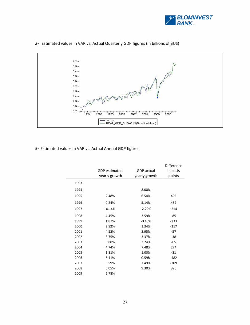
2- Estimated values in VAR vs. Actual Quarterly GDP figures (in billions of $US)

3- Estimated values in VAR vs. Actual Annual GDP figures

GDP estimated yearly growth

GDP actual yearly growth

Difference in basis points

1993

1994 8.00%

1995 2.48% 6.54% 405

1996 0.24% 5.14% 489

1997 -0.14% -2.29% -214

1998 4.45% 3.59% -85

1999 1.87% -0.45% -233

2000 3.52% 1.34% -217

2001 4.53% 3.95% -57

2002 3.75% 3.37% -38

2003 3.88% 3.24% -65

2004 4.74% 7.48% 274

2005 1.81% 1.00% -81

2006 5.41% 0.59% -482

2007 9.59% 7.49% -209

2008 6.05% 9.30% 325

2009 5.78%

28

S A L

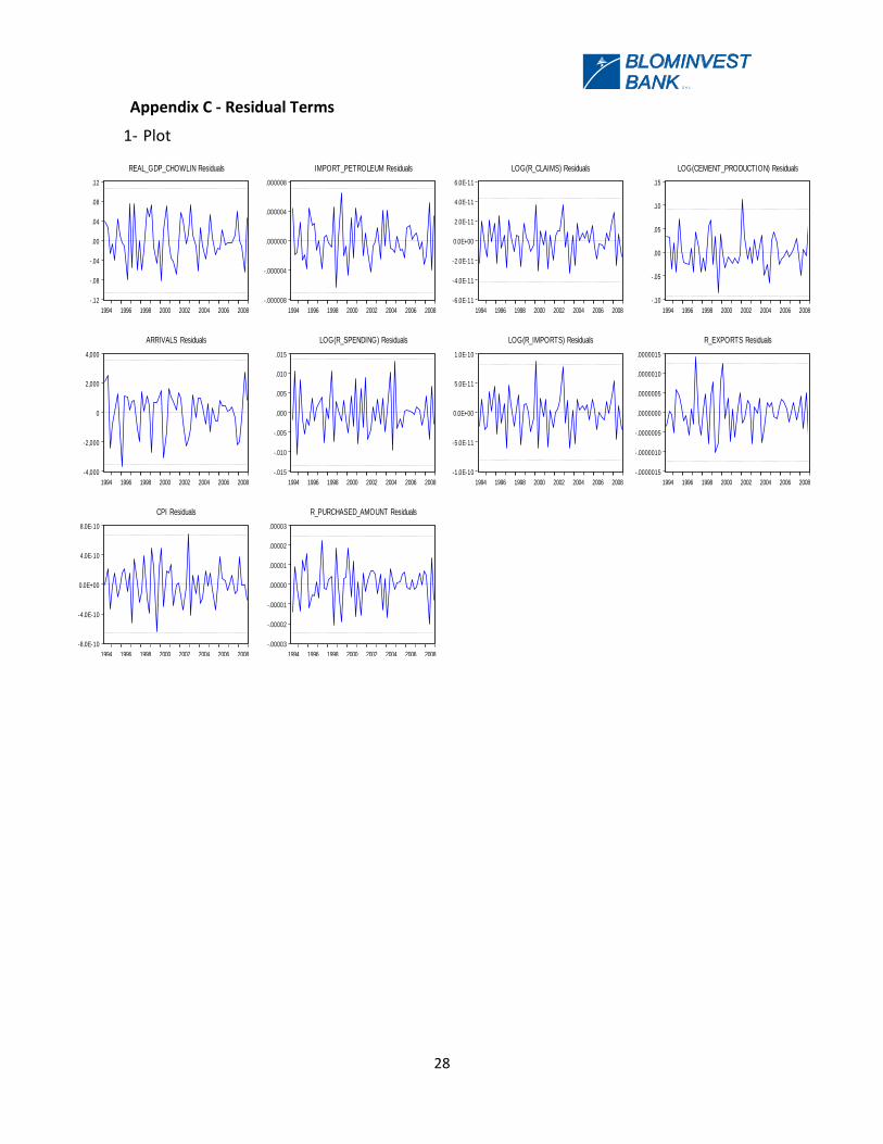
Appendix C - Residual Terms

1- Plot

-.12

-.08

-.04

.00

.04

.08

.12

1994 1996 1998 2000 2002 2004 2006 2008

REAL_GDP_CHOWLIN Residuals

-.000008

-.000004

.000000

.000004

.000008

1994 1996 1998 2000 2002 2004 2006 2008

IMPORT_PETROLEUM Residuals

-6.0E-11

-4.0E-11

-2.0E-11

0.0E+00

2.0E-11

4.0E-11

6.0E-11

1994 1996 1998 2000 2002 2004 2006 2008

LOG(R_CLAIMS) Residuals

-.10

-.05

.00

.05

.10

.15

1994 1996 1998 2000 2002 2004 2006 2008

LOG(CEMENT_PRODUCTION) Residuals

-4,000

-2,000

0

2,000

4,000

1994 1996 1998 2000 2002 2004 2006 2008

ARRIVALS Residuals

-.015

-.010

-.005

.000

.005

.010

.015

1994 1996 1998 2000 2002 2004 2006 2008

LOG(R_SPENDING) Residuals

-1.0E-10

-5.0E-11

0.0E+00

5.0E-11

1.0E-10

1994 1996 1998 2000 2002 2004 2006 2008

LOG(R_IMPORTS) Residuals

-.0000015

-.0000010

-.0000005

.0000000

.0000005

.0000010

.0000015

1994 1996 1998 2000 2002 2004 2006 2008

R_EXPORTS Residuals

-8.0E-10

-4.0E-10

0.0E+00

4.0E-10

8.0E-10

1994 1996 1998 2000 2002 2004 2006 2008

CPI Residuals

-.00003

-.00002

-.00001

.00000

.00001

.00002

.00003

1994 1996 1998 2000 2002 2004 2006 2008

R_PURCHASED_AMOUNT Residuals

29

S A L