Estimating overlap of daily activity patterns from … overlap of daily activity patterns from...
23
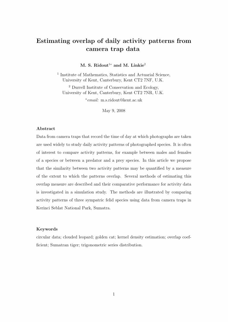
Estimating overlap of daily activity patterns from camera trap data M. S. Ridout 1* and M. Linkie 2 1 Institute of Mathematics, Statistics and Actuarial Science, University of Kent, Canterbury, Kent CT2 7NF, U.K. 2 Durrell Institute of Conservation and Ecology, University of Kent, Canterbury, Kent CT2 7NR, U.K. * email: [email protected] May 9, 2008 Abstract Data from camera traps that record the time of day at which photographs are taken are used widely to study daily activity patterns of photographed species. It is often of interest to compare activity patterns, for example between males and females of a species or between a predator and a prey species. In this article we propose that the similarity between two activity patterns may be quantified by a measure of the extent to which the patterns overlap. Several methods of estimating this overlap measure are described and their comparative performance for activity data is investigated in a simulation study. The methods are illustrated by comparing activity patterns of three sympatric felid species using data from camera traps in Kerinci Seblat National Park, Sumatra. Keywords circular data; clouded leopard; golden cat; kernel density estimation; overlap coef- ficient; Sumatran tiger; trigonometric series distribution. 1
-
Upload
hoangthien -
Category
Documents
-
view
215 -
download
1
Transcript of Estimating overlap of daily activity patterns from … overlap of daily activity patterns from...
Estimating overlap of daily activity patterns from
camera trap data
M. S. Ridout1∗ and M. Linkie2
1 Institute of Mathematics, Statistics and Actuarial Science,University of Kent, Canterbury, Kent CT2 7NF, U.K.
2 Durrell Institute of Conservation and Ecology,University of Kent, Canterbury, Kent CT2 7NR, U.K.
∗email: [email protected]
May 9, 2008
Abstract
Data from camera traps that record the time of day at which photographs are taken
are used widely to study daily activity patterns of photographed species. It is often
of interest to compare activity patterns, for example between males and females
of a species or between a predator and a prey species. In this article we propose
that the similarity between two activity patterns may be quantified by a measure
of the extent to which the patterns overlap. Several methods of estimating this
overlap measure are described and their comparative performance for activity data
is investigated in a simulation study. The methods are illustrated by comparing
activity patterns of three sympatric felid species using data from camera traps in
Kerinci Seblat National Park, Sumatra.
Keywords
circular data; clouded leopard; golden cat; kernel density estimation; overlap coef-
ficient; Sumatran tiger; trigonometric series distribution.
1
1 Introduction
Tropical rain forests contain some of the highest levels of species diversity and
abundance, but many tropical species are cryptic, shy and secretive, which makes
them notoriously difficult to study. Consequently, these species, and their interac-
tions with one another, remain poorly understood. This is the case especially for
medium-large bodied rainforest carnivores.
Camera trap surveys provide one important source of data on these species. Typ-
ically, camera traps record the date and time at which each photograph is taken,
allowing analysis of activity patterns with much improved precision over physical
traps used for small mammals, which can be visited only infrequently, and typ-
ically pinpoint activity only within a range of a few hours (e.g. Rychlik, 2005).
Nonetheless, camera trap times are commonly presented by grouping the capture
times into hourly, two-hourly of occasionally irregular intervals (Jacomo, Silveira
and Diniz-Filho, 2004). As in other contexts, it may be preferable to present kernel
density estimates, for reasons discussed by Wand and Jones (1995, Section 1.2), for
example.
In this paper we consider how to quantify the temporal overlap between pairs of
activity patterns. Comparisons of interest might include predator and prey species
(e.g. Weckel, Guiliano and Silver, 2006) or males and females of a species (e.g. Di
Bitetti, Paviolo and De Angelo, 2006).
We regard the observed capture times as random samples from underlying ab-
solutely continuous distributions and seek measures of overlap between the proba-
bility density functions (p.d.f.s) of these distributions. We focus on one particular
measure of overlap, the coefficient of overlapping, and estimate this nonparametri-
cally using kernel density estimates, following the approach of Schmid and Schmidt
(2006). The key difference here is that the recorded variable, time-of-day, is a circu-
lar random variable whose underlying density may well be bimodal. The precision
of the estimator of overlap is estimated by bootstrapping.
2
To illustrate the methodology, we investigate temporal activity pattern overlap of
three sympatric carnivore species, tiger (Panthera tigris), clouded leopard (Neofelis
diardi) and golden cat (Catopuma temminckii), from four camera trap study areas
in Kerinci Seblat National Park, Sumatra. Previous studies have speculated that the
clouded leopard alters its behaviour according to competition with larger carnivores
and may even be less nocturnal in Borneo, where other large carnivores, such as
tiger, are absent (Davis, 1962; Rabinowitz et al., 1987). However, a more important
potential source of interspecific competition may exist between the similar-sized
clouded leopard (11-20 kg) and golden cat (9-15 kg) (Nowell and Jackson, 1996).
Camera trap studies are now providing data with which these species interactions
can be investigated.
The paper is organised as follows. In Section 2 we discuss briefly some measures
of overlap. In Section 3 we discuss nonparametric estimation of the coefficient of
overlapping, including details of the kernel density estimation procedure when the
data are circular. Section 4 presents some results from a simulation study that
investigates the effect of different choices of bandwidth and Section 5 presents the
results of the analysis of the data from Kerinci Seblat National Park.
2 Measures of overlap
Many different measures have been suggested for quantifying the affinity or overlap
of two probability density functions f(x) and g(x). Examples include
∆(f, g) =∫
min {f(x), g(x)} dx (Weitzman, 1970),
ρ(f, g) =∫ √
f(x)g(x)dx (Matusita, 1955),
λ(f, g) = 2∫f(x)g(x)dx/
{∫[f(x)]2dx+
∫[g(x)]2dx
}(Morisita, 1959).
The notation and attributions here follow Mulekar and Mishra (2000). Because
fields of application are diverse, these measures have often been re-invented and
analogous measures, with integrals replaced by sums, have also been proposed for
measuring overlap of discrete distributions. In the specific context of measuring
3
overlap of ecological niches, these and other measures are discussed, for example,
by Hurlbert (1978) and by Slobodchikoff and Schulz (1980).
Measures of overlap are often related to well-known measures of distance between
densities. For example, ∆(f, g) is related to the L1 distance between the densities,
∆(f, g) = 1 −1
2
∫|f(x) − g(x)|dx
and ρ is similarly related to the Hellinger distance. A useful survey of distance
measures is provided by Devroye (1987; Chapter 1), which includes, for example, a
proof of LeCam’s inequality
∆(f, g) ≥1
2ρ(f, g)2.
In this paper, we focus on ∆(f, g) and write this simply as ∆ unless we wish to
clarify the densities involved. This measure, which is known as the coefficient of
overlapping, has the advantage of being a natural measure of overlap that is easily
interpreted geometrically. A probabilistic interpretation is that for any (Borel)
subset of times A, the difference in Pr(A) for the two distributions is at most 1−∆
(Devroye, 1987, Schmid and Schmidt, 2006). For any densities f(x) and g(x), ∆
lies in the interval [0, 1], with ∆ = 1 if and only if the densities are identical and
∆ = 0 if and only if f(x)g(x) = 0 for all x (Clemons and Bradley, 2000). For
activity patterns, ∆ = 0 could arise if one species was strictly diurnal and the other
strictly nocturnal, for example.
Another general advantage of this measure of overlap, which follows from its re-
lationship to L1 distance, is that it is invariant under strictly monotonic transfor-
mations (Devroye, 1987); if X and Y are random variables with p.d.f. f(x) and
g(x) respectively, and if ψ is a strictly monotonic function, then the overlapping
coefficient of ψ(X) and ψ(Y ) is the same as that of X and Y . Whilst this property
does not appear to have direct practical relevance to camera trap data, it does form
the basis of one of the alternative estimators of ∆ considered in Section 3 (Schmid
and Schmidt, 2006).
Finally, we note one simple property of ∆, that is a direct consequence of the fact
4

that L1 distance satisfies the triangle inequality and that is relevant to the example
in Section 6. Suppose that f(x) and g(x) are mixture densities of the form
f(x) =n∑
i=1
wifi(x) and g(x) =n∑
i=1
wigi(x),
where {fi(x)} and {gi(x)} are densities and∑n
i=1wi = 1. Then
n∑
i=1
wi∆(fi, gi) < ∆(f, g). (1)
3 Nonparametric estimation of ∆
In the absence of any strong prior belief about the parameteric form of the under-
lying densities f(x) and g(x), it is natural to consider estimating these measures of
overlap nonparametrically, by applying the measures to estimators f(x) and g(x)
of the densities f(x) and g(x). This approach, with the density estimators taken to
be kernel density estimators, is discussed by Ahmad (1980a), Ahmad (1980b) and
Clemons and Bradley (2000) for the measures λ, ρ and ∆, respectively.
Nonparametric estimation of ∆ is studied in more detail by Schmid and Schmidt
(2006), who note several equivalent mathematical expressions for ∆ which lead to
five different estimators. They establish the consistency of these estimators under
weak regularity conditions. We consider four of their estimators, excluding one
(OV L3 in their notation) which is not invariant to the choice of origin for circular
data.
Let x1, . . . , xn and y1, . . . , ym denote the two sets of sample times. For camera trap
data, the sample sizes m and n will usually differ. The four estimators that we
5
consider are defined as
∆1 =
∫1
0
min{f(t), g(t)
}dt (2)
∆2 = 1 −1
2
∫1
0
|f(t) − g(t)| dt (3)
∆4 =1
2
(1
n
n∑
i=1
min
{1,g (xi)
f (xi)
}+
1
m
m∑
j=1
min
{1,f (yj)
g (yj)
})(4)
∆5 =1
n
n∑
i=1
I{f(xi) < g(xi)
}+
1
m
m∑
j=1
I{g(yj) ≤ f(yj)
}, (5)
where I(.) is an indicator function and where the subscripts attached to the various
estimators match those of Schmid and Schmidt (2006). The integrals in equations
(2) and (3) are evaluated using the trapezoidal rule on a grid of 512 equally spaced
points. In general, this results in distinct estimators which, in the simulations
of Schmid and Schmidt (2006), sometimes had different properties. For circular
data, however, where the density is constrained to be equal at the endpoints of the
distribution, it can be shown that use of the trapezoidal rule gives identical values
for ∆1 and ∆2 and we therefore have just three distinct estimators to consider.
For any of these estimators we may estimate standard errors by the bootstrap. We
follow Clemons and Bradley (2000) and Schmid and Schmidt (2006) in using 200
bootstrap samples.
4 Estimating the densities f (x) and g(x)
The estimators of ∆ described in the previous section require estimators of the den-
sities f(x) and g(x). In keeping with earlier work, we concentrate on kernel density
estimators but, for comparison, we also consider estimating the densities within a
flexible parametric framework proposed recently by Fernandez-Duran (2004).
6
4.1 Kernel density estimation
Schmid and Schmidt (2006) use a Gaussian kernel with bandwidth h chosen by
Silverman’s (1986) rule, h = 1.06σn−1/5. Clemons and Bradley (2000) prefer the
alternative form of this rule in which σ is replaced by IQR/1.34 if this is less than
σ, where IQR is the interquartile range.
For circular data, we proceed analogously, using recent results of Taylor (2008).
We consider estimation of f(x) from the sample x1, x2, . . . , xn; estimation of g(x)
proceeds in the same way. The angle between an arbitrary point x in [0, 2π), and
the ith sample point is
a(x, xi) = min (|x− xi|, 2π − |x− xi|)
and the angular distance between the points is then
d(x, xi) = 1 − cos[a(x, xi)],
(Jammalamadaka and SenGupta, 2001, p. 17). The kernel density estimator that
we consider has the form
f(x; ν) =1
n
n∑
i=1
Kν [d(x, xi)]
where Kν is the p.d.f. of the von Mises distribution with mode at zero and concen-
tration parameter ν (Jammalamadaka and SenGupta, 2001, Section 12.9).
As usual in kernel density estimation, a critical issue is the choice of the smoothing
parameter, represented here by the von Mises concentration parameter ν (roughly
analogous to 1/h2 in the case of a Gaussian kernel). Taylor (2008) shows that if
the data arise from a von Mises distribution with concentration parameter κ, then
the asymptotic integrated mean squared error (AMISE) is minimised by choosing
ν =
[3nκ2I2(2κ)
4π1/2I0(κ)2
]2/5
, (6)
where Ir(.) is the modified Bessel function of order r. Taylor (2008) then considers
various ways of calculating a suitable robust estimate of κ to plug into equation (6)
7
when the underlying distribution may not be a von Mises distribution. One simple
approach that generally works quite well in Taylor’s simulations is to let
κ = max{κk, k = 1, . . . , K},
where the estimators κk are solutions of the equations
Ak(κ) =1
n
n∑
i=1
cos(kxi − µk),
where Ak(κ) = Ik(κ)/I0(κ) and where µk is the direction of kth sample trigono-
metric moment (Jammalamadaka and SenGupta, 2001, Section 1.3). If the data
are from a von Mises distribution with concentration parameter κ then κ1 is the
maximum likelihood estimate of κ and values of κk for k > 1 should be similar. But
if the underlying distribution is not von Mises, the estimators κk are expected to
differ (Taylor, 2008).
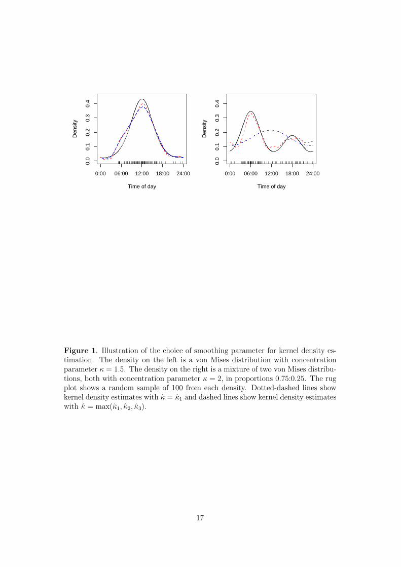
This is illustrated in Figure 1, which shows two densities, one representing a species
that is predominantly diurnal and the other a species that is crepuscular, with
greater activity around sunrise than around sunset. The solid lines in the plots
represent the true density and the rug plot indicates a random sample of size 100
from this density that was used to calculate kernel density estimates. We set K = 3
and plotted kernel density estimates from choosing κ = κ1 and κ = max(κ1, κ2, κ3).
In both examples, the latter choice gave κ = κ3. For the unimodal distribution, the
choice of κ made little difference to the resulting density estimate. For the bimodal
distribution, setting κ = κ1 gave a very poor estimate, whereas κ = κ3 captured
the main features of the bimodal distribution.
4.2 Estimation by non-negative trigonometric sums
Fernandez-Duran (2004) has proposed a class of circular distributions with proba-
bility density function of the form
f(t) =1
2π+
1
π
P∑
p=1
{ap cos(2πpt) + bp sin(2πpt)} (0 ≤ t ≤ 1). (7)
8

Somewhat complicated restrictions on the parameters {ap} and {bp} are required
to ensure that the density remains non-negative. However, for a given value of
P , maximum likelihood estimates of {ap} and {bp} may be calculated numerically.
Our experience is that the likelihood surface often has multiple local optima and
it is therefore important to run the numerical optimisation multiple times, from
different starting values, to try to ensure that the global optimum has been found.
As a result, fitting the distribution requires much more computation time than
kernel density estimation. It is also necessary to choose an appropriate value of P .
Fernandez-Duran (2004) suggests choosing P to minimize the Akaike information
criterion (AIC). There may be more than one local minimum of AIC as a function
of P and in numerical work we have chosen the smallest local minimum. Once the
densities are estimated, calculation of the various estimators of overlap proceeds as
in Section 3; examples are provided in Section 6.
5 Simulation study
Figure 2 shows twelve hypothetical activity patterns chosen to represent types of
activity likely to be encountered in practice. Those in the first column represent
species that are active primarily during the day; they differ in the strength of the
day time peak and the extent to which a reduced level of activity occurs during the
night. The distributions in the second column of Figure 2 are identical to those in
the first column, except that times have been shifted by twelve hours. Thus the roles
of day and night are interchanged. The final column shows patterns for crepuscular
species, with two peaks of activity; they differ in the strength and symmetry of
the peaks. The 66 distinct pairs that can be formed from these distributions have
overlap coefficients ranging from 0.015 to 0.862.
We conducted a simulation study to investigate the performance of the estimators
∆1, ∆4 and ∆5 when f(x) and g(x) were estimated by kernel density estimation.
The ‘optimal’ value of the concentration parameter of the von Mises kernel, νopt,
was calculated from equation (6), with κ = max(κ1, κ2, κ3) substituted for κ. One
9
objective of the simulations was to investigate the effect of under- or over-smoothing
on the resulting estimators of overlap and we therefore set the concentration pa-
rameter of the kernel to be c νopt for various values of c. Note that because ν is
a concentration parameter, c < 1 represents over-smoothing and c > 1 represents
under-smoothing, relative to the use of νopt.
For each of the 66 pairs of distributions, we investigated the effect of sample size
(n = m = 25, 50, 100 or 200) and the choice of c (= 0.1, 0.25, 0.5, 0.75, 1, 1.25, 1.5,
2 or 4) on the bias and precision of the resulting estimators of overlap. We ran
100 simulations for each combination of factors. Comparable simulations with f(x)
and g(x) estimated by trigonometric sum distributions were not run because they
would have required a huge amount of computer time.
Each set of 100 simulations was summarised by the bias, standard deviation and
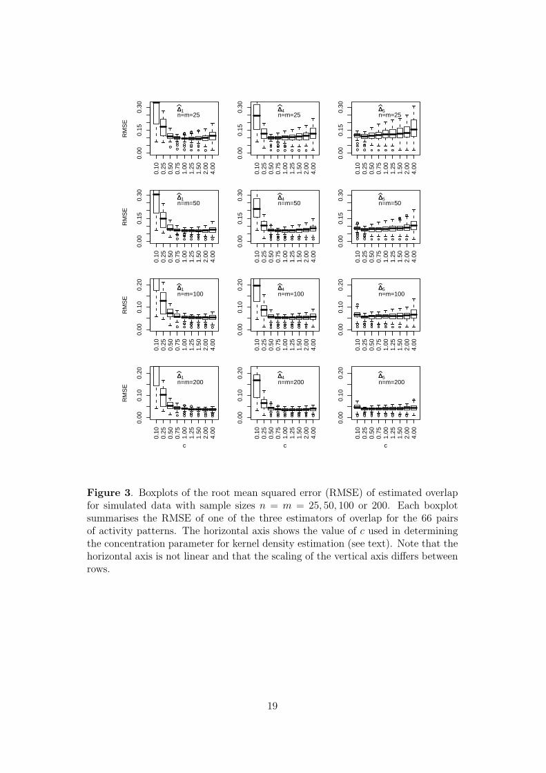
root mean square error (RMSE) of the 100 estimates. Figure 3 shows boxplots of the
RMSE across the 66 pairs of distributions. Often, the best distribution of RMSE
values occurs for values of c other than c = 1 but the patterns differ markedly. For
∆1 and ∆4, the optimal choice of c increases with sample size, whereas for ∆5 it is
consistently around c = 0.25.
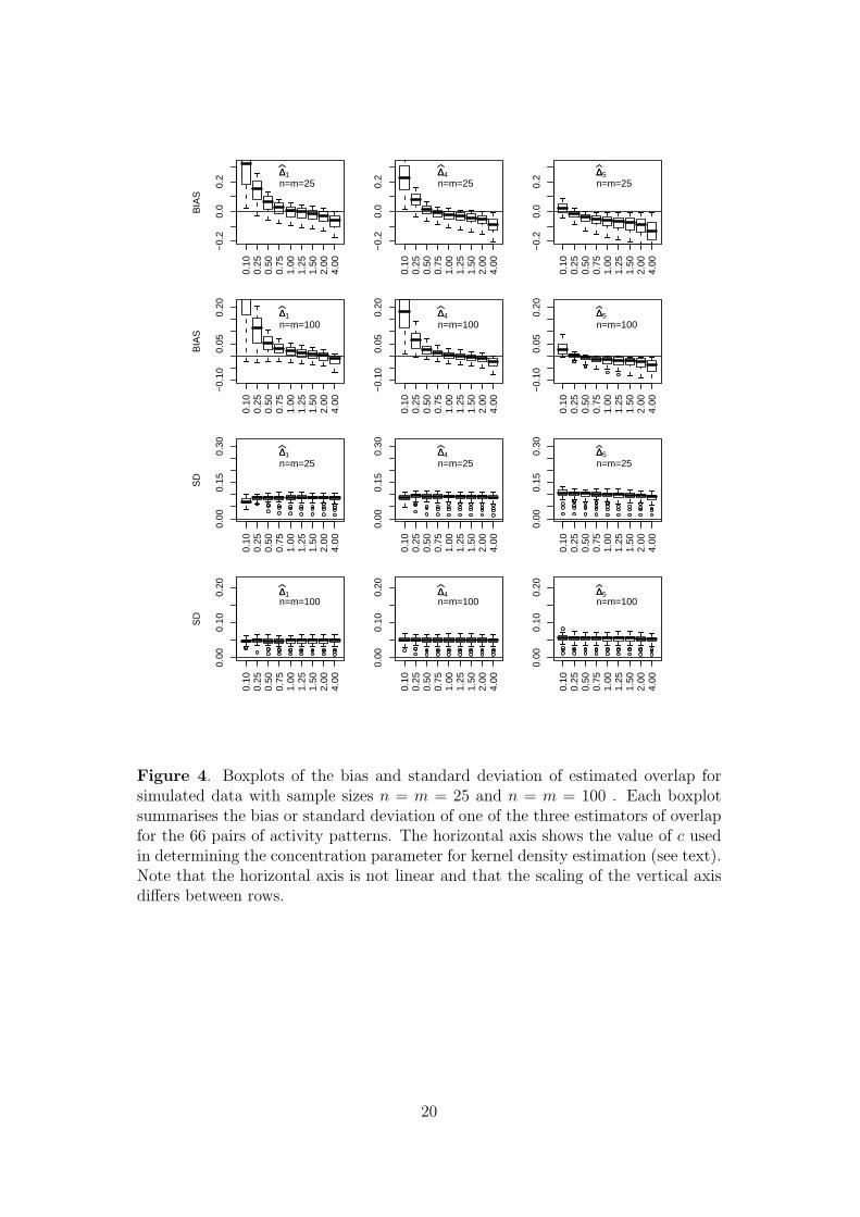
Figure 4 shows that the patterns arise predominantly due to changing bias, with
the standard deviation being relatively insensitive to the choice of c. When c < 1
the data are over-smoothed and in the limit as c→ 0, the kernel density estimates
will approach uniform distributions, with ∆ = 1. Conversely, when c is large the
kernel estimates are concentrated around the individual data points, resulting in
underestimation of ∆. Consequently, we anticipate that the bias will be a decreasing
function of c, as is seen in Figure 4. However, the magnitude and rate of decline of
the bias depend on the estimator.
Figure 5 compares the estimators for fixed values of c = 1.25 for ∆1, c = 1.0 for ∆4
and c = 0.25 for ∆5. These choices of c perform reasonably well across the range of
sample sizes considered in the simulations. The left hand panels of Figure 5 show
10
that for small sample sizes ∆1 is generally preferable to ∆4, in terms of RMSE,
whereas the converse is true for large sample sizes. The central and right hand
panels of Figure shows that, for each sample size, the better of these two estimators
generally outperforms ∆5.
6 Application to felid species in Kerinci Seblat
National Park
The methods described above were applied to camera trap records from four study
areas located in and around the 13,300km2 Kerinci Seblat National Park. Across
the four areas, data were recorded from 138 camera trap placements over a total of
8984 trap days. Photographs that were recorded within thirty minutes of a previous
photograph at the same site were excluded from the data set because of concerns
about lack of independence.
A previous analysis of some of the data from these traps (Linkie et al., 2008) esti-
mated overlap of the activity pattern of the Sumatran tiger with activity patterns of
four ungulate species considered to be tiger prey using the estimator ∆2 (equivalent
to ∆1), though based on a different method of kernel density estimation to that
described above. Here we apply the methods described in this paper to estimate
activity overlap of the Sumatran tiger and two other felid species, the Asian golden
cat and the clouded leopard.
Table 1 shows the number of records of each species in each study area. We begin
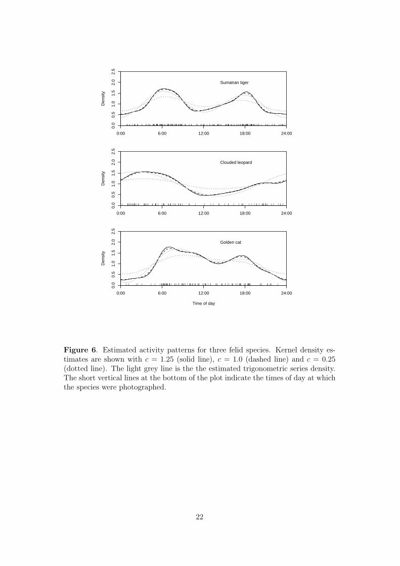
by considering the combined data from all four study areas. Figure 6 shows kernel
density estimates with c = 1.25, c = 1.0 and c = 0.25 and estimated trigonometric
sum densities, obtained by minimising AIC, as described in Section 4.2, which gave
P = 2 for tiger and clouded leopard and P = 1 for golden cat. Kernel density
estimates with c = 1.25 or c = 1 are quite similar to the estimated trigonometric
sum densities, but compared to these the kernel density estimate with c = 0.25
appears substantially undersmoothed.
11
Based on the results of the previous Section, we used the kernel density estimates
with c = 1.25, c = 1.0 and c = 0.25 to calculate the estimators ∆1, ∆4 and
∆5, respectively. We also calculated these estimators using the trigonometric sum
estimators of density. The results, shown in Table 2, indicate a high degree of
overlap between tiger and golden cat and, to a lesser extent between tiger and
clouded leopard, but a considerably lower level of overlap between golden cat and
clouded leopard. For the relatively large sample sizes involved here, the simulation
results of the previous Section suggest that ∆4 may be the most reliable estimator.
Whilst these analyses are useful for illustrating the methodology, they are poten-
tially misleading, because the distributions of times appear to differ between areas,
based, for example, on the test using circular ranks given in Section 5.3.6 of Fisher
(1993). In particular, for clouded leopards, there is a marked difference between
areas 2 and 4, where the animal appears predominantly nocturnal, and sites 1 and
3, where there are several day time observations.
Table 3 therefore provides estimates of overlap for each site separately. Because
sample sizes at individual sites are often small (Table 1), we use the estimator ∆1,
with c = 1.25. For tiger and golden cat, the estimates for areas 2, 3 and 4 are all
similar, but the estimate for area 1 is much smaller. However, this latter estimate is
based on very small samples at both sites, as reflected by its larger standard error.
When comparing clouded leopard with either tiger or golden cat, the differences
between areas in the capture times of clouded leopards are now reflected in the
estimates of overlap, which are lower for areas 2 and 4.
The inequality (1) involving mixture distributions at the end of Section 2 implies
that the values of overlap obtained for the data pooled across areas will exceed the
average value for the separate areas. The numerical results in Table 3 show that
the effect is quite substantial, so that pooling the data across sites substantially
overestimates the extent of overlap within areas.
12
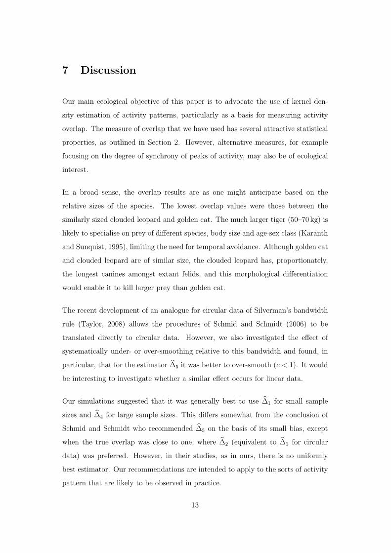
7 Discussion
Our main ecological objective of this paper is to advocate the use of kernel den-
sity estimation of activity patterns, particularly as a basis for measuring activity
overlap. The measure of overlap that we have used has several attractive statistical
properties, as outlined in Section 2. However, alternative measures, for example
focusing on the degree of synchrony of peaks of activity, may also be of ecological
interest.
In a broad sense, the overlap results are as one might anticipate based on the
relative sizes of the species. The lowest overlap values were those between the
similarly sized clouded leopard and golden cat. The much larger tiger (50–70 kg) is
likely to specialise on prey of different species, body size and age-sex class (Karanth
and Sunquist, 1995), limiting the need for temporal avoidance. Although golden cat
and clouded leopard are of similar size, the clouded leopard has, proportionately,
the longest canines amongst extant felids, and this morphological differentiation
would enable it to kill larger prey than golden cat.
The recent development of an analogue for circular data of Silverman’s bandwidth
rule (Taylor, 2008) allows the procedures of Schmid and Schmidt (2006) to be
translated directly to circular data. However, we also investigated the effect of
systematically under- or over-smoothing relative to this bandwidth and found, in
particular, that for the estimator ∆5 it was better to over-smooth (c < 1). It would
be interesting to investigate whether a similar effect occurs for linear data.
Our simulations suggested that it was generally best to use ∆1 for small sample
sizes and ∆4 for large sample sizes. This differs somewhat from the conclusion of
Schmid and Schmidt who recommended ∆5 on the basis of its small bias, except
when the true overlap was close to one, where ∆2 (equivalent to ∆1 for circular
data) was preferred. However, in their studies, as in ours, there is no uniformly
best estimator. Our recommendations are intended to apply to the sorts of activity
pattern that are likely to be observed in practice.
13
An alternative to kernel density estimation is to fit parametric distributions. Here
we have explored the use of trigonometric sum distributions (Fernandez-Duran,
2004), which gave similar results to the kernel density based estimates in our exam-
ples. Directional log-spline distributions (Ferreira, Juarez and Steel, 2008) might
provide a useful alternative if more flexibility is required in the shape of the activity
pattern.
Acknowledgements
We are grateful to the US Fish and Wildlife Service, 21st Century Tiger, RuffordSmall Grants and the Peoples Trust for Endangered Species for funding this work.We are grateful to Ir. Soewartono, Dr Sugardjito and the Department of Forestryand Nature Protection for assisting us in our Indonesian work and to Yoan Dinata,Agung Nugroho and Iding Achmad Haidir for their help with the data collection.We also thank Juan Fernandez-Duran for helpful discussion of trigonometric seriesdistributions and Miguel Juarez for providing the software for fitting directionallog-spline distributions.
References
Ahmad, I.A. (1980a). Nonparametric estimation of an affinity measure between twoabsolutely continuous distributions with hypothesis testing applications. Annals
of the Institute of Statistical Mathematics, 32, 223–240.
Ahmad, I.A. (1980b). Nonparametric estimation of Matusita’s measure of affinitybetween absolutely continuous distributions. Annals of the Institute of Statisti-
cal Mathematics, 32, 241–245.
Clemons, T.E. and Bradley, E. L. (2000) A nonparametric measure of the over-lapping coefficient. Computational Statistics and Data Analysis, 34, 51–61.(Erratum: 36, 243).
Davis, D.D. (1962) Mammals of the lowland rain-forest of North Borneo. Bulletin
of the Singapore Natural History Museum, 31, 1–129.
Devroye, L. (1987) A Course in Density Estimation. Boston: Birkhauser.
Di Bitetti, M.S., Paviolo, A. and De Angelo, C. (2006) Density, habitat use and ac-tivity patterns of ocelots (Leopardus pardalis) in the Atlantic Forest of Misiones,Argentina. Journal of Zoology, 270, 153–163.
Fernandez-Duran, J.J. (2004) Circular distributions based on nonnegative trigono-metric sums. Biometrics, 60, 499–503.
14
Ferreira, J.T.A.S., Juarez, M.A. and Steel, M.F. (2008) Directional log-spline dis-tributions. Bayesian Analysis, 3, 1–19.
Fisher, N.I. (1993) Statistical Analysis of Circular Data. Cambridge: CambridgeUniversity Press.
Hurlbert, S.H. (1978) The measurement of niche overlap and some relatives. Ecol-
ogy, 59, 67–77.
Jacomo, A.T.A., Silveira, L., Diniz-Filho, J.A.F. (2004) Niche separation betweenthe maned wolf (Chrysocyon brachyurus), the crab-eating fox (Dusicyon thous)and the hoary fox (Dusicyon vetulus) in central Brazil. Journal of Zoology, 262,99–106.
Jammalamadaka, S. and SenGupta, A. (2001) Topics in Circular Statistics. Singa-pore: World Scientific.
Karranth, K.U. and Sunquist, M.E. (1995) Prey selection by tiger, leopard anddhole in tropical forests. Journal of Animal Ecology, 64, 439–450.
Linkie, M., Borysiewicz, R.S., Dinata, Y., Nugroho, A., Achmad Haidir, I., Ridout,M.S., Leader-Williams, N. and Morgan, B.J.T. (2008) Predicting the spatio-temporal patterns of tiger and their prey across a primary-disturbed forest land-scape in Sumatra. Submitted for publication.
Matusita, K. (1955) Decision rules, based on the distance, for problems of fit, twosamples, and estimation. Annals of Mathematical Statistics, 26, 631–640.
Morisita, M. (1959) Measuring interspecific association and similarity between com-munities. Memoirs of the Faculty of Science of Kyushu Univeristy, Series E,
Biology, 3, 65–80.
Mulekar, M.S. and Mishra S.N. (2000) Confidence interval estimation of overlap:equal means case. Computational Statistics and Data Analysis, 34, 121–137.
Nowell, K. and Jackson, P. (1996) Wild Cats – Status Survey and Conservation
Action Plan. Gland, Switzerland: IUCN.
Rabinowitz, A.R., Andau, P. and Chai, P.P.K. (1987) The clouded leopard inMalaysian Borneo. Oryx, 21, 107-111.
Rychlik, L. (2005) Overlap of temporal niches among four sympatric species ofshrews. Acta Theriologica, 50, 175–188.
Schmid, F. and Schmidt, A. (2006) Nonparametric estimation of the coefficient ofoverlapping — theory and empirical application. Computational Statistics and
15

Data Analysis, 50, 1583–1596.
Silverman, B. (1986) Density Estimation for Statistics and Data Analysis. NewYork: Chapman and Hall.
Slobodchikoff, C.N. and Schulz, W.C. (1980) Measures of niche overlap. Ecology,61, 1051-1055.
Taylor, C.C. (2008) Automatic bandwidth selection for circular density estimation.Computational Statistics and Data Analysis, 52, 3493–3500.
Wand, M.P. and Jones, M.C. (2005) Kernel Smoothing London: Chapman andHall.
Weckel, M., Giuliano, W. and Silver, S. (2006) Jaguar (Panthera onca), feedingecology: distribution of predator and prey through time and space. Journal of
Zoology, 270, 25–30.
Weitzman, M.S. (1970) Measure of the overlap of income distribution of white andNegro families in the United States. Technical Report No. 22, U.S. Departmentof Commerce, Bureau of the Census, Washington, DC.
16
0.0
0.1
0.2
0.3
0.4
Time of day
Den
sity
0:00 06:00 12:00 18:00 24:00
0.0
0.1
0.2
0.3
0.4
Time of day
Den
sity
0:00 06:00 12:00 18:00 24:00
Figure 1. Illustration of the choice of smoothing parameter for kernel density es-timation. The density on the left is a von Mises distribution with concentrationparameter κ = 1.5. The density on the right is a mixture of two von Mises distribu-tions, both with concentration parameter κ = 2, in proportions 0.75:0.25. The rugplot shows a random sample of 100 from each density. Dotted-dashed lines showkernel density estimates with κ = κ1 and dashed lines show kernel density estimateswith κ = max(κ1, κ2, κ3).
17

01
23
45
Den
sity
0:00 12:00 24:00
(a)
01
23
45
0:00 12:00 24:00
(b)
01
23
45
0:00 12:00 24:00
(c)0
12
34
5
Den
sity
0:00 12:00 24:00
(d)
01
23
45
0:00 12:00 24:00
(e)
01
23
45
0:00 12:00 24:00
(f)
01
23
45
Den
sity
0:00 12:00 24:00
(g)
01
23
45
0:00 12:00 24:00
(h)
01
23
45
0:00 12:00 24:00
(i)
01
23
45
Time of day
Den
sity
0:00 12:00 24:00
(j)
01
23
45
Time of day
0:00 12:00 24:00
(k)
01
23
45
Time of day
0:00 12:00 24:00
(l)
Figure 2. Twelve hypothetical activity patterns. Figures (a), (b), (d), (e), (j) and(k) are von Mises distributions; figures (c), (f), (i) and (l) are mixtures of two vonMises distributions; figures (g) and (h) are wrapped Cauchy distributions.
18
0.00
0.15
0.30
RM
SE
0.10
0.25
0.50
0.75
1.00
1.25
1.50
2.00
4.00
∆∆1n=m=25
0.00
0.15
0.30
0.10
0.25
0.50
0.75
1.00
1.25
1.50
2.00
4.00
∆∆4n=m=25
0.00
0.15
0.30
0.10
0.25
0.50
0.75
1.00
1.25
1.50
2.00
4.00
∆∆5n=m=25
0.00
0.15
0.30
RM
SE
0.10
0.25
0.50
0.75
1.00
1.25
1.50
2.00
4.00
∆∆1n=m=50
0.00
0.15
0.30
0.10
0.25
0.50
0.75
1.00
1.25
1.50
2.00
4.00
∆∆4n=m=50
0.00
0.15
0.30
0.10
0.25
0.50
0.75
1.00
1.25
1.50
2.00
4.00
∆∆5n=m=50
0.00
0.10
0.20
RM
SE
0.10
0.25
0.50
0.75
1.00
1.25
1.50
2.00
4.00
∆∆1n=m=100
0.00
0.10
0.20
0.10
0.25
0.50
0.75
1.00
1.25
1.50
2.00
4.00
∆∆4n=m=100
0.00
0.10
0.20
0.10
0.25
0.50
0.75
1.00
1.25
1.50
2.00
4.00
∆∆5n=m=100
0.00
0.10
0.20
c
RM
SE
0.10
0.25
0.50
0.75
1.00
1.25
1.50
2.00
4.00
∆∆1n=m=200
0.00
0.10
0.20
c
0.10
0.25
0.50
0.75
1.00
1.25
1.50
2.00
4.00
∆∆4n=m=200
0.00
0.10
0.20
c
0.10
0.25
0.50
0.75
1.00
1.25
1.50
2.00
4.00
∆∆5n=m=200
Figure 3. Boxplots of the root mean squared error (RMSE) of estimated overlapfor simulated data with sample sizes n = m = 25, 50, 100 or 200. Each boxplotsummarises the RMSE of one of the three estimators of overlap for the 66 pairsof activity patterns. The horizontal axis shows the value of c used in determiningthe concentration parameter for kernel density estimation (see text). Note that thehorizontal axis is not linear and that the scaling of the vertical axis differs betweenrows.
19
−0.
20.
00.
2
BIA
S
0.10
0.25
0.50
0.75
1.00
1.25
1.50
2.00
4.00
∆∆1n=m=25
−0.
20.
00.
2
0.10
0.25
0.50
0.75
1.00
1.25
1.50
2.00
4.00
∆∆4n=m=25
−0.
20.
00.
2
0.10
0.25
0.50
0.75
1.00
1.25
1.50
2.00
4.00
∆∆5n=m=25
−0.
100.
050.
20
BIA
S
0.10
0.25
0.50
0.75
1.00
1.25
1.50
2.00
4.00
∆∆1n=m=100
−0.
100.
050.
20
0.10
0.25
0.50
0.75
1.00
1.25
1.50
2.00
4.00
∆∆4n=m=100
−0.
100.
050.
20
0.10
0.25
0.50
0.75
1.00
1.25
1.50
2.00
4.00
∆∆5n=m=100
0.00
0.15
0.30
SD
0.10
0.25
0.50
0.75
1.00
1.25
1.50
2.00
4.00
∆∆1n=m=25
0.00
0.15
0.30
0.10
0.25
0.50
0.75
1.00
1.25
1.50
2.00
4.00
∆∆4n=m=25
0.00
0.15
0.30
0.10
0.25
0.50
0.75
1.00
1.25
1.50
2.00
4.00
∆∆5n=m=25
0.00
0.10
0.20
SD
0.10
0.25
0.50
0.75
1.00
1.25
1.50
2.00
4.00
∆∆1n=m=100
0.00
0.10
0.20
0.10
0.25
0.50
0.75
1.00
1.25
1.50
2.00
4.00
∆∆4n=m=100
0.00
0.10
0.20
0.10
0.25
0.50
0.75
1.00
1.25
1.50
2.00
4.00
∆∆5n=m=100
Figure 4. Boxplots of the bias and standard deviation of estimated overlap forsimulated data with sample sizes n = m = 25 and n = m = 100 . Each boxplotsummarises the bias or standard deviation of one of the three estimators of overlapfor the 66 pairs of activity patterns. The horizontal axis shows the value of c usedin determining the concentration parameter for kernel density estimation (see text).Note that the horizontal axis is not linear and that the scaling of the vertical axisdiffers between rows.
20
0.0 0.2 0.4 0.6 0.8
−0.
040.
000.
04
Diff
eren
cen=m=25
0.0 0.2 0.4 0.6 0.8
−0.
040.
000.
04 n=m=25
0.0 0.2 0.4 0.6 0.8
−0.
040.
000.
04 n=m=25
0.0 0.2 0.4 0.6 0.8
−0.
040.
000.
04
Diff
eren
ce
n=m=50
0.0 0.2 0.4 0.6 0.8
−0.
040.
000.
04 n=m=25
0.0 0.2 0.4 0.6 0.8
−0.
040.
000.
04 n=m=50
0.0 0.2 0.4 0.6 0.8
−0.
030.
000.
03
Diff
eren
ce
n=m=100
0.0 0.2 0.4 0.6 0.8
−0.
040.
000.
04 n=m=25
0.0 0.2 0.4 0.6 0.8
−0.
030.
000.
03 n=m=100
0.0 0.2 0.4 0.6 0.8
−0.
020.
000.
02
True overlap value
Diff
eren
ce
n=m=200
0.0 0.2 0.4 0.6 0.8
−0.
040.
000.
04
True overlap value
n=m=25
0.0 0.2 0.4 0.6 0.8
−0.
020.
000.
02
True overlap value
n=m=200
Figure 5. Differences in root mean square error (RMSE) values between estima-
tors. The left hand column shows RMSE(∆4) − RMSE(∆1), the middle column
shows RMSE(∆5) − RMSE(∆1), and the right hand column shows RMSE(∆5) −
RMSE(∆4). Different rows show different sample sizes, as indicated on the graphs.
We set c = 1.25 for calculating ∆1, c = 1.0 for calculating ∆4 and c = 0.25 forcalculating ∆5. Different symbols in the plots indicate different types of activitypattern for which the overlap was estimated; either both distributions were uni-modal (circle), both were bimodal (square) or one was unimodal and the other wasbimodal (triangle).
21
0.0
0.5
1.0
1.5
2.0
2.5
Den
sity
0:00 6:00 12:00 18:00 24:00
Sumatran tiger
0.0
0.5
1.0
1.5
2.0
2.5
Den
sity
0:00 6:00 12:00 18:00 24:00
Clouded leopard
0.0
0.5
1.0
1.5
2.0
2.5
Time of day
Den
sity
0:00 6:00 12:00 18:00 24:00
Golden cat
Figure 6. Estimated activity patterns for three felid species. Kernel density es-timates are shown with c = 1.25 (solid line), c = 1.0 (dashed line) and c = 0.25(dotted line). The light grey line is the the estimated trigonometric series density.The short vertical lines at the bottom of the plot indicate the times of day at whichthe species were photographed.
22
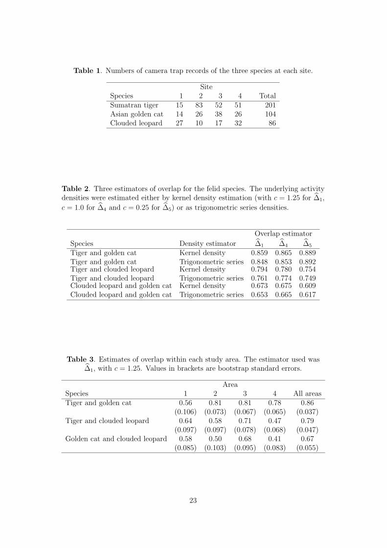
Table 1. Numbers of camera trap records of the three species at each site.
SiteSpecies 1 2 3 4 TotalSumatran tiger 15 83 52 51 201Asian golden cat 14 26 38 26 104Clouded leopard 27 10 17 32 86
Table 2. Three estimators of overlap for the felid species. The underlying activitydensities were estimated either by kernel density estimation (with c = 1.25 for ∆1,
c = 1.0 for ∆4 and c = 0.25 for ∆5) or as trigonometric series densities.
Overlap estimator
Species Density estimator ∆1 ∆4 ∆5
Tiger and golden cat Kernel density 0.859 0.865 0.889Tiger and golden cat Trigonometric series 0.848 0.853 0.892Tiger and clouded leopard Kernel density 0.794 0.780 0.754Tiger and clouded leopard Trigonometric series 0.761 0.774 0.749Clouded leopard and golden cat Kernel density 0.673 0.675 0.609Clouded leopard and golden cat Trigonometric series 0.653 0.665 0.617
Table 3. Estimates of overlap within each study area. The estimator used was∆1, with c = 1.25. Values in brackets are bootstrap standard errors.
AreaSpecies 1 2 3 4 All areasTiger and golden cat 0.56 0.81 0.81 0.78 0.86
(0.106) (0.073) (0.067) (0.065) (0.037)Tiger and clouded leopard 0.64 0.58 0.71 0.47 0.79
(0.097) (0.097) (0.078) (0.068) (0.047)Golden cat and clouded leopard 0.58 0.50 0.68 0.41 0.67
(0.085) (0.103) (0.095) (0.083) (0.055)
23