METHODS ARTICLEpublished: 08 May 2014

doi: 10.3389/fninf.2014.00048

Estimating neural response functions from fMRISukhbinder Kumar1,2 and William Penny1*

1 Wellcome Trust Centre for Neuroimaging, University College London, London, UK2 Medical School, Institute of Neuroscience, Newcastle University, Newcastle, UK

Edited by:

Friedrich T. Sommer, University ofCalifornia at Berkeley, USA

Reviewed by:

Thomas Wennekers, University ofPlymouth, UKXin Wang, The Salk Institute forBiological Studies, USA

*Correspondence:

William Penny, Wellcome TrustCentre for Neuroimaging, UniversityCollege London, 12 Queen Square,London WC1N 3BG, UKe-mail: w.penny@ucl.ac.uk

This paper proposes a methodology for estimating Neural Response Functions (NRFs)from fMRI data. These NRFs describe non-linear relationships between experimentalstimuli and neuronal population responses. The method is based on a two-stage modelcomprising an NRF and a Hemodynamic Response Function (HRF) that are simultaneouslyfitted to fMRI data using a Bayesian optimization algorithm. This algorithm also producesa model evidence score, providing a formal model comparison method for evaluatingalternative NRFs. The HRF is characterized using previously established “Balloon” andBOLD signal models. We illustrate the method with two example applications based onfMRI studies of the auditory system. In the first, we estimate the time constants ofrepetition suppression and facilitation, and in the second we estimate the parametersof population receptive fields in a tonotopic mapping study.

Keywords: neural response function, population receptive field, parametric modulation, Bayesian inference,

auditory perception, repetition suppression, Tonotopic Mapping, Balloon model

1. INTRODUCTIONFunctional Magnetic Resonance Imaging (fMRI) is a well estab-lished technique for the non-invasive mapping of human brainfunction (Frackowiak et al., 2003). Analysis of fMRI data mostoften proceeds by modeling the neuronal correlates of singleevents as delta functions or boxcars. These form event streamswhich are then convolved with assumed Hemodynamic ResponseFunctions (HRFs) to create regressors for General Linear Models(GLMs). This forms the basis of the widely used StatisticalParametric Mapping (SPM) approach (Friston et al., 2007).

This paper proposes an alternative approach in which fMRIdata is fitted using a non-linear model depicted in Figure 1.This comprises two mappings (1) a Neural Response Function(NRF) which maps stimulus characteristics to neural responsesand (2) an HRF which maps neural responses to fMRI data.Importantly, the HRF can accommodate variations across brainregions and subjects, and includes non-linearities associated withhemodynamic saturation effects. The parameters of the twomappings are estimated together using a Bayesian optimiza-tion algorithm that is widely used in neuroimaging (Fristonet al., 2007). This algorithm has the added benefit of produc-ing a model evidence score which we will use to provide aformal model comparison method (Penny, 2012) for evaluatingalternative NRFs.

The goal of our approach is to make inferences about NRFs.These parametric models relate the activity of a population ofneurons within a single voxel or brain region to characteristicsof experimental stimuli. NRFs are similar, in principle, to thosederived for individual neurons from single unit electrophysiol-ogy but estimate population rather than single neuron responses(Dumoulin and Wandell, 2008). In this paper we apply the NRFapproach to the auditory domain and provide two examples.The first is a Repetition Suppression paradigm in which we esti-mate neural responses as a function of time since presentation

of a similar stimulus. These repetition suppression effects arean important marker of synaptic plasticity (Weigelt et al., 2008;Marta et al., 2009). The second is a Tonotopic Mapping paradigmin which we model neural responses as Gaussian or Mexican-Hatfunctions of stimulus frequency, and report the results of a formalBayesian model comparison.

This paper is based on a previous Hemodynamic Model(HDM) (Friston, 2002), which posited categorical relationsbetween stimuli and neural activation, and used a biophysi-cally motivated differential equation model of the HRF, whichin turn was based on earlier physiological modeling (Buxtonet al., 1998). This paper can be viewed as a simple extension ofthat work which replaces the categorical neuronal model with aparametric one.

A further perspective on this paper is that it presents an exten-sion of linear models with “Parametric Modulation” terms, inwhich experimental variables of interest are used to modulatethe height or duration of boxcar functions representing neu-ronal activity (Buchel et al., 1998; Grinband et al., 2008). Thework in this paper represents an extension of this approachby allowing for non-linear relations between fMRI signals andunknown parametric variables. Non-linear relationships can alsobe accommodated in the linear framework by using a Taylorseries approach, but this has a number of disadvantages whichare described in section 2.

2. MATERIALS AND METHODSFigure 1 shows the structure of the model proposed in thispaper. An NRF specifies how neuronal activity is related to stim-ulus characteristics and an HRF specifies how fMRI data isrelated to neuronal activity. The HRF is based on the Balloonmodel (Buxton et al., 1998) which describes how blood deoxy-hemoglobin, q, and volume, v, are driven by neuronal activity,and a BOLD signal model which describes how the BOLD signal

Frontiers in Neuroinformatics www.frontiersin.org May 2014 | Volume 8 | Article 48 | 1

NEUROINFORMATICS

Kumar and Penny Estimating neural response functions from fMRI

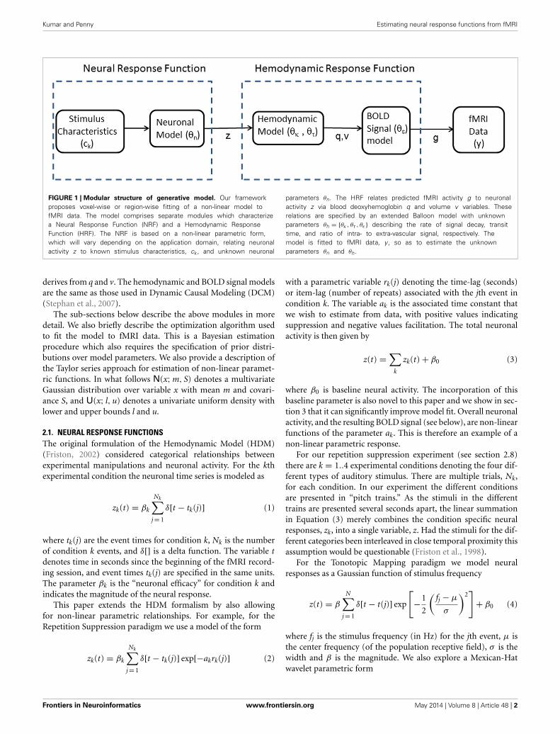
FIGURE 1 | Modular structure of generative model. Our frameworkproposes voxel-wise or region-wise fitting of a non-linear model tofMRI data. The model comprises separate modules which characterizea Neural Response Function (NRF) and a Hemodynamic ResponseFunction (HRF). The NRF is based on a non-linear parametric form,which will vary depending on the application domain, relating neuronalactivity z to known stimulus characteristics, ck , and unknown neuronal

parameters θn. The HRF relates predicted fMRI activity g to neuronalactivity z via blood deoxyhemoglobin q and volume v variables. Theserelations are specified by an extended Balloon model with unknownparameters θh = {θκ , θτ , θε } describing the rate of signal decay, transittime, and ratio of intra- to extra-vascular signal, respectively. Themodel is fitted to fMRI data, y , so as to estimate the unknownparameters θn and θh.

derives from q and v. The hemodynamic and BOLD signal modelsare the same as those used in Dynamic Causal Modeling (DCM)(Stephan et al., 2007).

The sub-sections below describe the above modules in moredetail. We also briefly describe the optimization algorithm usedto fit the model to fMRI data. This is a Bayesian estimationprocedure which also requires the specification of prior distri-butions over model parameters. We also provide a description ofthe Taylor series approach for estimation of non-linear paramet-ric functions. In what follows N(x; m, S) denotes a multivariateGaussian distribution over variable x with mean m and covari-ance S, and U(x; l, u) denotes a univariate uniform density withlower and upper bounds l and u.

2.1. NEURAL RESPONSE FUNCTIONSThe original formulation of the Hemodynamic Model (HDM)(Friston, 2002) considered categorical relationships betweenexperimental manipulations and neuronal activity. For the kthexperimental condition the neuronal time series is modeled as

zk(t) = βk

Nk∑j = 1

δ[t − tk(j)] (1)

where tk(j) are the event times for condition k, Nk is the numberof condition k events, and δ[] is a delta function. The variable tdenotes time in seconds since the beginning of the fMRI record-ing session, and event times tk(j) are specified in the same units.The parameter βk is the “neuronal efficacy” for condition k andindicates the magnitude of the neural response.

This paper extends the HDM formalism by also allowingfor non-linear parametric relationships. For example, for theRepetition Suppression paradigm we use a model of the form

zk(t) = βk

Nk∑j = 1

δ[t − tk(j)] exp[−akrk(j)] (2)

with a parametric variable rk(j) denoting the time-lag (seconds)or item-lag (number of repeats) associated with the jth event incondition k. The variable ak is the associated time constant thatwe wish to estimate from data, with positive values indicatingsuppression and negative values facilitation. The total neuronalactivity is then given by

z(t) =∑

k

zk(t) + β0 (3)

where β0 is baseline neural activity. The incorporation of thisbaseline parameter is also novel to this paper and we show in sec-tion 3 that it can significantly improve model fit. Overall neuronalactivity, and the resulting BOLD signal (see below), are non-linearfunctions of the parameter ak. This is therefore an example of anon-linear parametric response.

For our repetition suppression experiment (see section 2.8)there are k = 1..4 experimental conditions denoting the four dif-ferent types of auditory stimulus. There are multiple trials, Nk,for each condition. In our experiment the different conditionsare presented in “pitch trains.” As the stimuli in the differenttrains are presented several seconds apart, the linear summationin Equation (3) merely combines the condition specific neuralresponses, zk, into a single variable, z. Had the stimuli for the dif-ferent categories been interleaved in close temporal proximity thisassumption would be questionable (Friston et al., 1998).

For the Tonotopic Mapping paradigm we model neuralresponses as a Gaussian function of stimulus frequency

z(t) = β

N∑j = 1

δ[t − t(j)] exp

[−1

2

(fj − μ

σ

)2]

+ β0 (4)

where fj is the stimulus frequency (in Hz) for the jth event, μ isthe center frequency (of the population receptive field), σ is thewidth and β is the magnitude. We also explore a Mexican-Hatwavelet parametric form

Frontiers in Neuroinformatics www.frontiersin.org May 2014 | Volume 8 | Article 48 | 2

Kumar and Penny Estimating neural response functions from fMRI

z(t) = β

N∑j = 1

δ[t − t(j)][

1 −(

fj − μ

σ

)2]

exp

[−1

2

(fj − μ

σ

)2]

+ β0 (5)

This function, also referred to as a Ricker wavelet, is equivalentto the (negative, normalized) second derivative of a Gaussianfunction (Mallat, 1999). The function corresponds to a Gaussianwith surround suppression and can also be produced using aDifference of Gaussians (DoG) functional form (with specificparameter settings). Population receptive fields with surroundsuppression have been explored in the visual domain (Lee et al.,2013). Overall neuronal activity, and the resulting BOLD signal(see below), are non-linear functions of the parameters μ andσ . This is therefore another example of a non-linear parametricresponse. For the Tonotopic Mapping data we treat all stimuli asbelonging to the same category, so have dropped the k subscriptsin Equations (4, 5).

Although this paper focusses on the auditory system, we envis-age that our approach may also be useful for many other types ofneuroimaging study. So, generally we allow for NRFs of the form

z(t) = f (c1, c2, . . . , cK; θn) (6)

where ck are stimulus characteristics for conditions k = 1 . . . Kand f is an arbitrary linear or non-linear function with param-eters θn. For our Repetition Suppression example the neuronalparameters are θn = {ak, βk, β0} and for the Tonotopic Mappingexample they are θn = {μ, σ, β, β0} (here μ, σ and β are specifiedindirectly by Gaussian latent variables to allow for an appropri-ately constrained optimization, as described in section 2.3 below).More generally, the functional form is to be provided by themodeler and the parameters are to be estimated, as describedbelow. Different NRFs (e.g., Gaussian versus Mexican-Hat) canthen be evaluated in relation to each other using Bayesian ModelComparison (Penny, 2012).

2.2. HEMODYNAMICSNeuronal activity gives rise to fMRI data by a dynamic processdescribed by an extended Balloon model (Buxton et al., 2004)and BOLD signal model (Stephan et al., 2007) for each brainregion. This specifies how changes in neuronal activity give riseto changes in blood oxygenation that are measured with fMRI.

The hemodynamic model involves a set of hemodynamicstate variables, state equations and hemodynamic parameters, θh.Neuronal activity z causes an increase in vasodilatory signal s thatis subject to autoregulatory feedback and inflow fin responds inproportion to this

s = z − κs − γ (fin − 1) (7)

fin = s

Blood volume v and deoxyhemoglobin content q then changeaccording to the Balloon model

τ v = fin − fout (8)

τ q = finE(fin, ρ) − foutq

v

fout = v1/α (9)

where the first equation describes the filling of the venous“Balloon” until inflow equals outflow, fout , which happens withtime constant τ . The proportion of oxygen extracted from theblood is a function of flow

E(f , ρ) = 1 − (1 − ρ)1/f

ρ(10)

where ρ is resting oxygen extraction fraction. The free parametersof the model are the rate of signal decay in each region, κ , and thetransit time in each region, τ . The other parameters are fixed toγ = α = ρ = 0.32 in accordance with previous work (Stephanet al., 2007).

2.2.1. BOLD signal modelThe BOLD signal is given by a static non-linear function of vol-ume and deoxyhemoglobin that comprises a volume-weightedsum of extra- and intra-vascular signals. This is based on a simpli-fied approach (Stephan et al., 2007) (Equation 12) that improvesupon an earlier model (Friston et al., 2003)

y = V0

[k1(1 − q) + k2

(1 − q

v

)+ k3(1 − v)

](11)

k1 = 4.3θ0ρTE

k2 = εr0ρTE

k3 = 1 − ε

where V0 is resting blood volume fraction, θ0 is the frequencyoffset at the outer surface of the magnetized vessel for fully deoxy-genated blood at 1.5T, TE is the echo time and r0 is the slope of therelation between the intravascular relaxation rate and oxygen sat-uration (Stephan et al., 2007). In this paper we use the standardparameter values V0 = 4, r0 = 25, θ0 = 40.3 and for our fMRIimaging sequence we have TE = 0.04. The only free parameter ofthe BOLD signal model is ε, the ratio of intra- to extra-vascularsignal.

2.3. PRIORSThe overall model is fitted to data using the Variational Laplace(VL) optimization algorithm (Friston et al., 2007). This is aBayesian estimation procedure which requires the specificationof prior distributions over model parameters. The algorithm iswidely used in neuroimaging, finding applications ranging fromfitting of Equivalent Current Dipole source models to DCMs(Litvak et al., 2011). Within VL, priors must be specified asGaussians (see section 2.5). However, priors of any unimodalform can in effect be specified over variables of interest by usingGaussian latent variables and the appropriate non-linear trans-form. For example, we use uniform priors over parameters of theTonotopic models (see below).

Frontiers in Neuroinformatics www.frontiersin.org May 2014 | Volume 8 | Article 48 | 3

Kumar and Penny Estimating neural response functions from fMRI

2.3.1. Neural response functionIn the absence of other prior information about NRF param-eters we can initially use Gaussian priors with large variances,or uniform priors over a large range. Applying the optimizationalgorithm to selected empirical fMRI time series then providesus with ballpark estimates of parameter magnitudes. The priorscan then be set to reflect this experience (Gelman et al., 1995).Alternatively, one may be able to base these values on publisheddata from previous studies.

For the Repetition Suppression models used in this paper, weuse the following priors. The initial effect size has a Gaussian prior

p(βk) = N(βk; 1, σ 2

β

)(12)

with σ 2β = 10, and the decay coefficient also has a Gaussian prior

p(ak) = N(ak; 0, σ 2

a

)(13)

with σ 2a = 1. The baseline neuronal activity also has a Gaussian

prior

p(β0) = N(β0; 0, σ 2

β

)(14)

For the Tonotopic Mapping examples we used uniform priorsover the center frequency, width, and amplitude as follows

p(μ) = U(μ;μmin, μmax) (15)

p(σ ) = U(σ ; σmin, σmax)

p(β) = U(β;βmin, βmax)

The minimum and maximum values were μmin = 0, μmax =20, 000, σmin = 1, σmax = 5, 000, βmin = 0, βmax = 20. The cen-ter frequency and width are expressed in Hz. These uniformpriors were instantiated in the VL framework by specifying aGaussian latent variable and relating model parameters to latentvariables via the required non-linearity. We used

μ = (μmax − μmin)�(θμ) + μmin (16)

σ = (σmax − σmin)�(θσ ) + σmin

β = (βmax − βmin)�(θβ) + βmin

The priors over the latent variables θμ, θσ , and θβ were standardGaussians (zero mean, unit variance). The required non-linearity� was therefore set to the standard cumulative Gaussian func-tion (Wackerley et al., 1996). The prior over β0 was given byEquation (14).

In summary, for the Repetition Suppression example the neu-ronal parameters are θn = {ak, βk, β0} and for the TonotopicMapping example they are θn = {θμ, θσ , θβ, β0}.2.3.2. Hemodynamic response functionThe unknown parameters are {κ, τ, ε}. These are represented as

κ = 0.64 exp(θκ ) (17)

τ = 2 exp(θτ )

ε = exp(θε)

and we have Gaussian priors

p(θκ ) = N(θκ ; 0, 0.135) (18)

p(θτ ) = N(θτ ; 0, 0.135)

p(θε) = N(θε; 0, 0.135)

where θh = {θκ , θτ , θε} are the hemodynamic parameters to beestimated. These priors are used for both the applications in thispaper and are identical to those used in DCM for fMRI.

2.4. INTEGRATIONOur overall parameter vector θ = {θn, θh} comprises neurody-namic and hemodynamic parameters. Numerical integration ofthe hemodynamic equations leads to a prediction of fMRI activ-ity comprising a single model prediction vector g(θ, m). This hasdimension [T × 1] where T is the number of fMRI scans (lengthof time series). The numerical integration scheme used in thispaper is the ode15s stiff integrator from Matlab’s ODE suite(Shampine and Reichelt, 1997).

2.5. OPTIMIZATIONThe VL algorithm can be used for Bayesian estimation of non-linear models of the form

y = g(θ, m) + e (19)

where y is the fMRI time series, g(θ, m) is a non-linear functionwith parameters θ , and m indexes assumptions about the NRF.For example, in the Repetition Suppression example below (seesection 3) m indexes “item-lag” or “time-lag” models, and in theTonotopic Mapping example m indexes Gaussian or Mexican-Hatparametric forms.

The term e denotes zero mean additive Gaussian noise. Thelikelihood of the data is

p(y|θ, λ, m) = N(y; g(θ, m), exp(λ)−1IT) (20)

with noise precision exp (λ) and p(λ|m) = N(λ; μλ, Sλ) withμλ = 0, Sλ = 1. Here IT denotes a dimension T identity matrix.These values are used in DCM (Penny, 2012) and have been set soas to produce data sets with signal to noise ratios that are typicalin fMRI.

The framework allows for Gaussian priors over modelparameters

p(θ |m) = N(θ; μθ , Cθ ) (21)

where μθ and Cθ have been set as described in the previoussection on priors.

These distributions allow one to write down an expression forthe joint log likelihood of data, parameters and hyperparameters

p(y, θ, λ|m) = p(y|θ, λ, m)p(θ |m)p(λ|m) (22)

Frontiers in Neuroinformatics www.frontiersin.org May 2014 | Volume 8 | Article 48 | 4

Kumar and Penny Estimating neural response functions from fMRI

The VL algorithm then assumes an approximate posterior densityof the following factorized form

q(θ, λ|y, m) = q(θ |y, m)q(λ|y, m) (23)

q(θ |y, m) = N(θ; mθ , Sθ )

q(λ|y, m) = N(λ; mλ, Sλ)

The parameters of these approximate posteriors are then iter-atively updated so as to minimize the Kullback-Leibler (KL)-divergence between the true and approximate posteriors. Thisis the basic principle underlying all variational approaches toapproximate Bayesian inference; that one chooses a factoriza-tion of the posterior and updates parameters of the factors (heremθ , Sθ , mλ, and Sλ) so as to minimize the KL-divergence. Readersunfamiliar with this general approach can find introductorymaterial in recent texts (Jaakola et al., 1998; Bishop, 2006). For theVL algorithm, this minimization is implemented by maximizingthe following “variational energies”

I(θ) =∫

L(θ, λ)q(λ|y, m)dλ (24)

I(λ) =∫

L(θ, λ)q(θ |y, m)dθ

where L(θ, λ) = log p(y, θ, λ|m). As the likelihood, priors, andapproximate posteriors are Gaussian the above integrals can becomputed analytically (Bishop, 2006). Maximization is effectedby first computing the gradient and curvature of the variationalenergies at the current parameter estimate, mθ (old). For example,for the parameters we have

jθ (i) = ∂I(θ)

∂θ(i)(25)

Hθ (i, j) = d2I(θ)

∂θ(i)∂θ(j)

where i and j index the ith and jth parameters, jθ is the gradi-ent vector and Hθ is the curvature matrix. These gradients andcurvatures are computed using central differences (Press et al.,1992). In recent work (Sengupta et al., in press) we have proposeda more efficient “adjoint method,” which computes gradients andcurvatures as part of the numerical integration process.

The estimate for the posterior mean is then given by

mθ (new) = mθ (old) − H−1θ jθ (26)

which is equivalent to a Newton update (Press et al., 1992). Inregions of parameter space near maxima the curvature is negativedefinite (hence the negative sign above). Equation (26) imple-ments a step in the direction of the gradient with a step sizegiven by the inverse curvature. Large steps are therefore takenin regions where the gradient changes slowly (low curvature)and small steps where it changes quickly (high curvature). In theSPM implementation (in the function spm_nlsi_GN.m fromhttp://www.fil.ion.ucl.ac.uk/spm/), the update

also incorporates a regularization term (Press et al., 1992).Readers requiring a complete description of this algorithm arereferred to Friston et al. (2007).

A key feature of our approach, in which neurodynamic andhemodynamic parameters are estimated together rather than ina sequential “two-step” approach, can be illustrated by a closerinspection of Equation (26). If we decompose the means, gra-dients and curvatures into neurodynamic and hemodynamicparts

mθ = [mn, mh]T (27)

jθ = [jn, jh]T

Hθ = [Hnn, Hnh; Hhn, Hhh]

then [using the Schur complement (Bishop, 2006)] we can writethe update for the neurodynamic parameters as

mn(new) = mn(old) −[

Hnn − HnhH−1hh Hhn

]−1jn (28)

whereas the equivalent second step of a two-step approachwould use

mn(new) = mn(old) − H−1nn jn (29)

Thus, the joint estimation procedure includes an additional termsuch that components of the data that are explained by hemody-namic variation are not attributed to a neuronal cause. If there isno correlation between hemodynamic and neuronal parametersthen Hnh = Hhn = 0 and this additional term disappears. This issimilar to the issue of how correlated predictors are dealt with inGeneral Linear Modeling (Christensen, 2002; Friston et al., 2007).

2.6. MODEL COMPARISONThe VL algorithm also computes the model evidence p(y|m)based on a free-energy approximation (Penny, 2012). Given mod-els m = i and m = j the Bayes factor for i versus j is then given byKass and Raftery (1995)

BFij = p(y|m = i)

p(y|m = j)(30)

When BFij > 1, the data favor model i over j, and when BFij < 1the data favor model j. If there are more than two models to com-pare then we can choose one as a reference and calculate Bayesfactors relative to that reference. A Bayes factor greater than 20 or,equivalently, a log Bayes factor greater than 3 is deemed strongevidence in favor of a model (Raftery, 1995). It is also possi-ble to compute Bayes factors using the Savage–Dickey method,which only requires fitting a single “grandfather” model (Pennyand Ridgway, 2013). The use of Bayes factors provides a Bayesianalternative to hypothesis testing using classical inference (Dienes,2011).

2.7. TAYLOR SERIES APPROXIMATIONPreviously in the neuroimaging literature a Taylor series approx-imation method has been used to estimate parameters thatrelate stimulus properties non-linearly to neuronal activity

Frontiers in Neuroinformatics www.frontiersin.org May 2014 | Volume 8 | Article 48 | 5

Kumar and Penny Estimating neural response functions from fMRI

(Buchel et al., 1998). One can apply this approach, for example,to estimating time constants in Repetition Suppression experi-ments. For example, if we take Equation (2) (but drop referenceto condition k for brevity) we have

z(t) = β

N∑j = 1

δ[t − t(j)] exp[−ar(j)] (31)

A first order Taylor series expansion (in the variable a) of theexponential function around an assumed value a0 then gives

FIGURE 2 | Repetition suppression paradigm. Stimuli were presented inepochs with periods of silence in between. Within each epoch, stimuli werepresented in “pitch-trains” or “noise-trains,” where a pitch-train containedbetween 1 and 6 stimuli of the same pitch, and noise-trains containedbetween 1 and 6 noise stimuli. Colors indicate the various types of pitchtrain: Random Interval Noise (RIN) (red), Harmonic Complex (HC) (green),Click Train (CT) (blue), and noise (yellow). The black rectangle represents aperiod of silence.

z(t) ≈ β

N∑j = 1

δ[t − t(j)] (exp[−a0r(j)]

− (a − a0)r(j) exp[−a0r(j)]) (32)

This can be written as

z(t) = β1z1(t) + β2z2(t) (33)

β1 = β

β2 = β(a − a0)

z1(t) =N∑

j = 1

δ[t − t(j)] exp[−a0r(j)]

z2(t) = −N∑

j = 1

δ[t − t(j)]r(j) exp[−a0r(j)]

Convolution of this activity then produces the predicted BOLDsignal

g(t) = β1x1(t) + β2x2(t) (34)

x1 = z1 ⊗ h

x2 = z2 ⊗ h

FIGURE 3 | Magnitude of initial response, βk averaged over sessions, for

conditions k = 1, 2, 3, 4 (Harmonic Complex—HC, Click Train—CT,

Random Interval Noise—RIN, Noise). The red error bars indicate the

standard deviations. Estimates are shown for the six regions of interest;TE10, TE11, and TE12 indicate primary, medial, and lateral regions of Heschl’sGyrus, and -L/-R indicates left/right hemisphere.

Frontiers in Neuroinformatics www.frontiersin.org May 2014 | Volume 8 | Article 48 | 6

Kumar and Penny Estimating neural response functions from fMRI

where h is the hemodynamic response function (assumedknown). This also assumes linear superposition (that the responseof a sum is the sum of responses). This linearized model can be fit-ted to fMRI data using a standard GLM framework, with designmatrix columns x1 and x2 and estimated regression coefficientsβ1, β2. The estimated time constant is then given by

a = β2

β1

+ a0 (35)

The drawbacks of this approach are (1) it assumes that a reason-ably accurate estimate of a can be provided (a0, otherwise theTaylor series approximation is invalid), (2) it assumes the hemo-dynamic response is known and fixed across voxels, (3) it assumeslinear superposition (e.g., neglecting possible hemodynamic sat-uration effects), and (4) inference is not straightforward as theparameter estimate is based on a ratio of estimated quantities.However, the great benefit of this approach is that estimationcan take place using the GLM framework, allowing efficientapplication to large areas of the brain.

2.8. REPETITION SUPPRESSION DATAThe experimental stimuli consisted of three pitch evoking stimuliwith different “timbres;” Regular Interval Noise (RIN), harmoniccomplex (HC), and regular click train (CT). Five different pitchvalues were used having fundamental frequencies equally spaced

on a log-scale from 100 to 300 Hz. The duration of each stimuluswas 1.5 s.

The RIN of a pitch value F0 was generated by first generatinga sample of white noise, delaying it by 1/F0 s and then adding itback to the original sample. This delay and add procedure wasrepeated 16 times to generate a salient pitch. The stimulus wasthen bandpass filtered to limit its bandwidth between 1000 and4000 Hz. New exemplars of white noise were used to generate RINstimuli that were repeated within trials.

The HC stimulus of fundamental frequency F0 was generatedby adding sinusoids of harmonic frequencies (multiples of F0) upto a maximum frequency (half the sampling rate) with phaseschosen randomly from a uniform distribution. The resultingsignal was then Bandpass filtered between 1000 and 4000 Hz.

The CT of rate F0 consisted of uniformly spaced bursts of clicks(click duration 0.1 ms) with interval duration (time betweenclicks) equal to 1/F0 s. This train of clicks was then bandpassfiltered between 1000 and 4000 Hz.

We also included spectrally matched white noise stimuli(Noise) which were bandlimited to the same frequency rangeas pitch stimuli. Different white noise exemplars were used togenerate each RIN and Noise stimulus.

Stimuli were presented in epochs with periods of silencein between, as shown in Figure 2. Within each epoch, stimuliwere presented in “pitch-trains” or “noise-trains,” where a pitch-train contained between 1 and 6 stimuli of the same pitch, and

FIGURE 4 | Magnitude of repetition suppression effect, ak averaged

over sessions, for conditions k = 1, 2, 3, 4 (Harmonic Complex—HC,

Click Train—CT, Random Interval Noise—RIN, Noise). The red errorbars indicate the standard deviations. Positive values indicate

suppression and negative values facilitation. Estimates are shown forthe six regions of interest; TE10, TE11, and TE12 indicate primary,medial, and lateral regions of Heschl’s Gyrus, and -L/-R indicatesleft/right hemisphere.

Frontiers in Neuroinformatics www.frontiersin.org May 2014 | Volume 8 | Article 48 | 7

Kumar and Penny Estimating neural response functions from fMRI

noise-trains contained between 1 and 6 noise stimuli. For the HCand RIN stimuli, although the pitch value remained the same ineach pitch-train, the low level acoustic structure varied over stim-uli. For the CT stimuli, however, the low level structures wereidentical.

All imaging data were collected on a Siemens 3 Tesla Allegrahead-only MRI scanner. The participant gave written consent andthe procedures were approved by the University College LondonEthics committee. Stimuli were presented as shown in Figure 2,with MRI data being continuously acquired from 30 slices cover-ing the superior temporal plane (TR = 1.8 s, TE = 30 ms, FA =90◦, isotropic voxel size = 3 mm). To ensure subjects attended tothe stimuli, they were asked to press a button at the start of eachsilent period. The scanning time was divided into 5 sessions, eachlasting about 12 min. A total of 1800 volumes were acquired (360per session).

After discarding the first 2 dummy images to allow for T1relaxation effects, images were realigned to the first volume.The realigned images were normalized to stereotactic space andsmoothed by an isotropic Gaussian kernel of 6 mm full-width athalf maximum.

Cytoarchitectonically, Heschl’s gyrus (HG) can be partitionedinto three different areas (Morosan et al., 2001): a primaryarea (TE10) surrounded by two medial (TE11) and lateralareas (TE12) (see Figure 11 in Morosan et al., 2001). To testwhether these three areas have different rates of adaptation to the

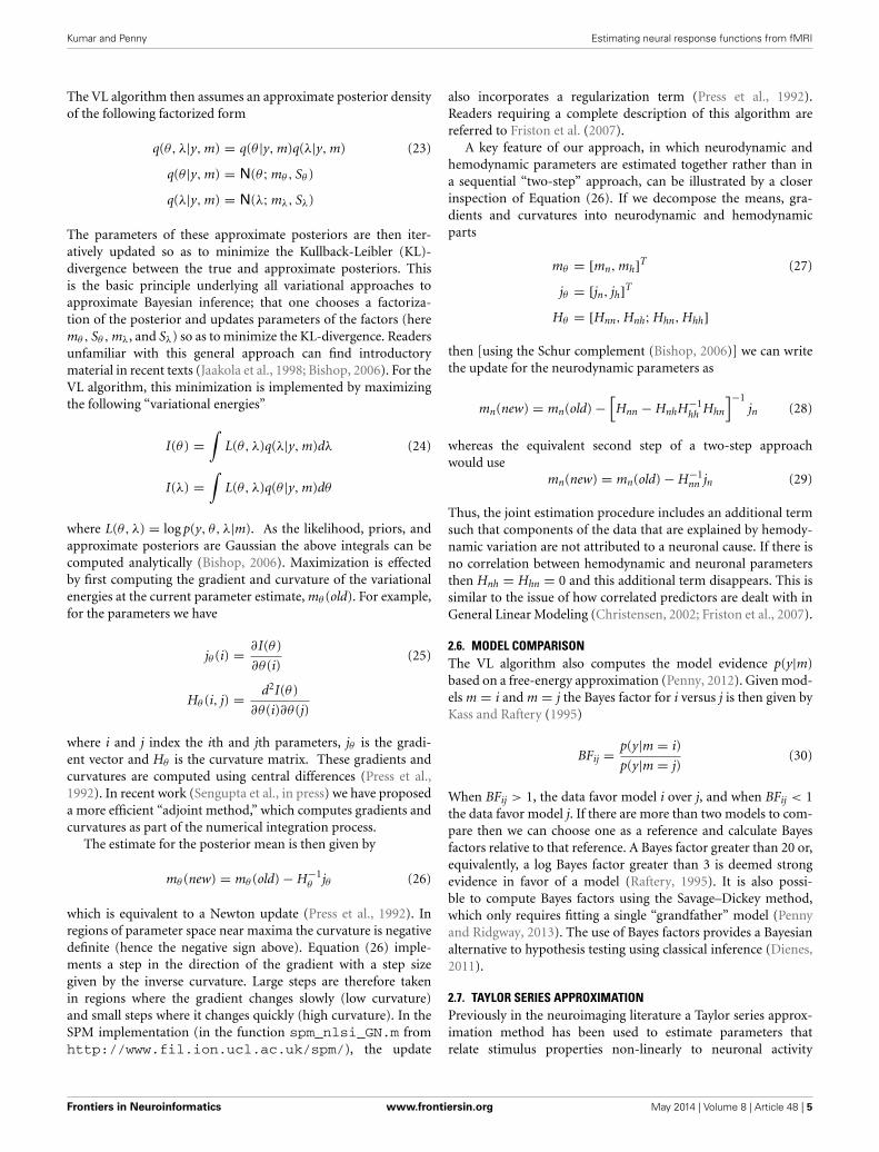
FIGURE 5 | Tonotopic Mapping with Gaussian neural response

functions. Top Left: Axial slice of structural image at z = 6 with boundingbox showing region displayed on other three panels (x, y, and z denote MNIcoordinates in mm). The labeling (A to F) refers to plots in Figures 6, 8. Top

Right: Amplitude β (arbitrary units), Bottom Left: Center Frequency μ (kHz).Bottom Right: Tuning, W (ratio of Center Frequency to FWHM).

repetition of pitch and noise stimuli, we extracted a time seriesfrom each of these areas. The anatomical mask of these areas,available in the anatomy toolbox (Eickhoff et al., 2005), were usedto define the ROIs. Principal component analysis was carried outto summarize multiple time series (from multiple voxels in a ROI)to a single time series by the first principal component.

It is well known that repeated presentation of a stimulusleads to adaptation of brain responses (Buckner et al., 1998;Grill-Spector et al., 1999). These neural adaptation or repetitionsuppression (RS) effects are described in a recent review (Weigeltet al., 2008). In this paper we tested for Repetition Suppressioneffects by estimating exponential neural response functions, asdescribed in section 3. We modeled neural activity as a functionof repetition number (“item-lag”) or repetition time (“time-lag”)within each epoch, and our aim was to estimate the associatedtime constant. Although stimuli varied in pitch this was neglectedfor the current analysis.

2.9. TONOTOPIC MAPPING DATAThe stimuli for the tonotopic mapping consisted of 14 pure tonesof frequencies: 88, 125, 177, 250, 354, 500, 707, 1000, 1414,2000, 2828, 4000, 5657, and 8000 Hz. Starting from a frequencyof 88 Hz, bursts of each tone were presented for 2 s after whichthe frequency was increased to the next highest frequency untilall 14 frequencies were presented in a single block of 28 s. Theblock of sound was followed by a 12 s silent period. This cycleof 40 s was repeated 15 times in a single session lasting 10 min.Stimuli were presented using sensimetrics earphones (http://www.sens.com/products/model-s14/) at a sampling rate of44,100 Hz.

Imaging data were acquired on Siemens 3 Tesla Quattro head-only MRI scanner. The MRI images were acquired continuouslyusing 3D MRI sequence (TR = 1.1 s, two echoes per image; TE1 =15.85 ms; TE2 = 34.39 ms; matrix size = 64 × 64). A total of 560volumes were acquired in one session. After the fMRI run, a highresolution (1 × 1 × 1 mm) T1-weighted structural MRI scan wasacquired. The two echoes of the images were first averaged. Theimages were then pre-processed in the same way as the RepetitionSuppression data. We restricted our data analysis to voxels froman axial slice (z = 6 mm) covering the superior temporal plane.

3. RESULTS3.1. REPETITION SUPPRESSIONWe report results on an exponential “item-lag” model, in whichneuronal responses were modeled using Equation (2), k indexesthe four stimulus types (HC, CT, RIN, Noise), and rk encodesthe number of item repeats since the first stimulus of that typein the epoch. We also fitted “time-lag” models which used thesame equation but where rk encoded the elapsed time (in seconds)since the first stimulus of that type in the epoch.

We first report a model comparison of the item-lag versus timelag models. Both model types were fitted to data from five ses-sions in six brain regions, giving a total of 30 data sets. The logmodel evidence was computed using a free energy approximationdescribed earlier. The difference in log model evidence was thenused to compute a log Bayes factor, with a value of 3 or greaterindicating strong evidence.

Frontiers in Neuroinformatics www.frontiersin.org May 2014 | Volume 8 | Article 48 | 8

Kumar and Penny Estimating neural response functions from fMRI

Strong evidence in favor of the “time-lag” model was found innone out of 30 data sets, strong evidence in favor of the “item-lag”model was found in 22 out of 30 data sets. In the remaining 8 datasets, the Bayes factors were not decisive but the item-lag modelwas preferred in 7 of them. We therefore conclude that item-lagsbetter capture the patterns in our data, and what follows belowrefers only to the item-lag models.

We now present results on the parametric responses of interestas captured by the βk (initial response) and ak (decay) variables.These are estimated separately for each session of data using themodel fitting algorithm described earlier. We then combine esti-mates over sessions using precision weighted averaging (Kasesset al., 2010). This is a Bayes-optimal procedure in which the over-all parameter estimate is given by a weighted average of individualsession estimates. The weights are given by the relative preci-sions (inverse variances) of the session estimates so that thosewith higher precision contribute more to the final parameterestimate.

The estimates of the initial response magnitudes, βk, areshown in Figure 3 and the estimates of the suppression effects,ak, are shown in Figure 4. Figure 3 shows that the pattern ofinitial responses (responses at item lag 0) is similar over allregions with CT and RIN typically eliciting the largest responses.Figure 4 shows that the noise stimulus does not elicit any repe-tition suppression effect in any region. The CT stimulus elicits a

suppression effect which is strongest in TE10-L whereas the HCstimulus elicits a facilitation effect in all regions.

3.2. TONOTOPIC MAPPINGThis section describes the estimation of Neural ResponseFunctions for the Tonotopic Mapping data. We first focus onthe Gaussian parametric form described in Equation (4). TheFull Width at Half Maximum is given by FWHM = 2

√(2 ln 2)σ .

Following Moerel et al. (2012) we define the Tuning Value asW = μ/FWHM where μ and FWHM are expressed in Hz. Largertuning values indicate more narrowly tuned response functions.

We restricted our data analysis to a single axial slice (z = 6)covering superior temporal plane. This slice contained 444 voxelsin the auditory cortex.

Figure 5 shows the parameters of a Gaussian NRF as esti-mated over this slice. The main characteristics are as follows. First,the center frequency decreases and then increases again as onemoves along the posterior to anterior axis with high frequenciesat y = −30, low frequencies at y = −10 and higher frequen-cies again at y = 5. There is a single region of high amplituderesponses that follows the length of Heschl’s Gyrus (the diagonalband in the top right panel of Figure 5). These responses have alow center frequency of between 200 and 300 Hz. Finally the tun-ing values are approximately constant over the whole slice, with avalue of about W = 1, except for a lateral posterior region with a

FIGURE 6 | Estimated Gaussian neural response functions at six selected voxels (voxel indices denote MNI coordinates in mm). The labeling (A – F)refers to positions shown in the top left panel of Figure 5.

Frontiers in Neuroinformatics www.frontiersin.org May 2014 | Volume 8 | Article 48 | 9

Kumar and Penny Estimating neural response functions from fMRI

much higher value of about W = 4. Figure 6 plots the estimatedGaussian response functions at six selected voxels.

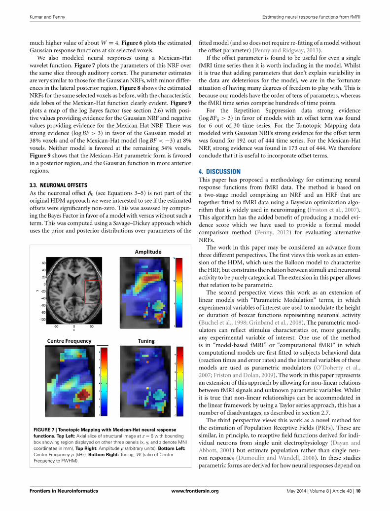
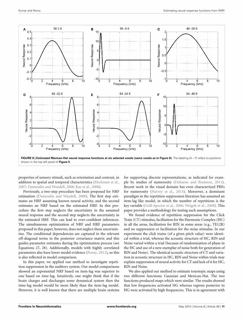
We also modeled neural responses using a Mexican-Hatwavelet function. Figure 7 plots the parameters of this NRF overthe same slice through auditory cortex. The parameter estimatesare very similar to those for the Gaussian NRFs, with minor differ-ences in the lateral posterior region. Figure 8 shows the estimatedNRFs for the same selected voxels as before, with the characteristicside lobes of the Mexican-Hat function clearly evident. Figure 9plots a map of the log Bayes factor (see section 2.6) with posi-tive values providing evidence for the Gaussian NRF and negativevalues providing evidence for the Mexican-Hat NRF. There wasstrong evidence (log BF > 3) in favor of the Gaussian model at38% voxels and of the Mexican-Hat model (log BF < −3) at 8%voxels. Neither model is favored at the remaining 54% voxels.Figure 9 shows that the Mexican-Hat parametric form is favoredin a posterior region, and the Gaussian function in more anteriorregions.

3.3. NEURONAL OFFSETSAs the neuronal offset β0 (see Equations 3–5) is not part of theoriginal HDM approach we were interested to see if the estimatedoffsets were significantly non-zero. This was assessed by comput-ing the Bayes Factor in favor of a model with versus without such aterm. This was computed using a Savage–Dickey approach whichuses the prior and posterior distributions over parameters of the

FIGURE 7 | Tonotopic Mapping with Mexican-Hat neural response

functions. Top Left: Axial slice of structural image at z = 6 with boundingbox showing region displayed on other three panels (x, y, and z denote MNIcoordinates in mm), Top Right: Amplitude β (arbitrary units). Bottom Left:

Center Frequency μ (kHz). Bottom Right: Tuning, W (ratio of CenterFrequency to FWHM).

fitted model (and so does not require re-fitting of a model withoutthe offset parameter) (Penny and Ridgway, 2013).

If the offset parameter is found to be useful for even a singlefMRI time series then it is worth including in the model. Whilstit is true that adding parameters that don’t explain variability inthe data are deleterious for the model, we are in the fortunatesituation of having many degrees of freedom to play with. This isbecause our models have the order of tens of parameters, whereasthe fMRI time series comprise hundreds of time points.

For the Repetition Suppression data strong evidence(log BFij > 3) in favor of models with an offset term was foundfor 6 out of 30 time series. For the Tonotopic Mapping datamodeled with Gaussian NRFs strong evidence for the offset termwas found for 192 out of 444 time series. For the Mexican-HatNRF, strong evidence was found in 173 out of 444. We thereforeconclude that it is useful to incorporate offset terms.

4. DISCUSSIONThis paper has proposed a methodology for estimating neuralresponse functions from fMRI data. The method is based ona two-stage model comprising an NRF and an HRF that aretogether fitted to fMRI data using a Bayesian optimization algo-rithm that is widely used in neuroimaging (Friston et al., 2007).This algorithm has the added benefit of producing a model evi-dence score which we have used to provide a formal modelcomparison method (Penny, 2012) for evaluating alternativeNRFs.

The work in this paper may be considered an advance fromthree different perspectives. The first views this work as an exten-sion of the HDM, which uses the Balloon model to characterizethe HRF, but constrains the relation between stimuli and neuronalactivity to be purely categorical. The extension in this paper allowsthat relation to be parametric.

The second perspective views this work as an extension oflinear models with “Parametric Modulation” terms, in whichexperimental variables of interest are used to modulate the heightor duration of boxcar functions representing neuronal activity(Buchel et al., 1998; Grinband et al., 2008). The parametric mod-ulators can reflect stimulus characteristics or, more generally,any experimental variable of interest. One use of the methodis in “model-based fMRI” or “computational fMRI” in whichcomputational models are first fitted to subjects behavioral data(reaction times and error rates) and the internal variables of thesemodels are used as parametric modulators (O’Doherty et al.,2007; Friston and Dolan, 2009). The work in this paper representsan extension of this approach by allowing for non-linear relationsbetween fMRI signals and unknown parametric variables. Whilstit is true that non-linear relationships can be accommodated inthe linear framework by using a Taylor series approach, this has anumber of disadvantages, as described in section 2.7.

The third perspective views this work as a novel method forthe estimation of Population Receptive Fields (PRFs). These aresimilar, in principle, to receptive field functions derived for indi-vidual neurons from single unit electrophysiology (Dayan andAbbott, 2001) but estimate population rather than single neu-ron responses (Dumoulin and Wandell, 2008). In these studiesparametric forms are derived for how neural responses depend on

Frontiers in Neuroinformatics www.frontiersin.org May 2014 | Volume 8 | Article 48 | 10

Kumar and Penny Estimating neural response functions from fMRI

FIGURE 8 | Estimated Mexican-Hat neural response functions at six selected voxels (same voxels as in Figure 6). The labeling (A – F) refers to positionsshown in the top left panel of Figure 5.

properties of sensory stimuli, such as orientation and contrast, inaddition to spatial and temporal characteristics (Heckman et al.,2007; Dumoulin and Wandell, 2008; Kay et al., 2008).

Previously, a two-step procedure has been proposed for NRFestimation (Dumoulin and Wandell, 2008). The first step esti-mates an HRF assuming known neural activity, and the secondestimates an NRF based on the estimated HRF. In this pro-cedure the first step neglects the uncertainty in the assumedneural response and the second step neglects the uncertainty inthe estimated HRF. This can lead to over-confident inferences.The simultaneous optimization of NRF and HRF parametersproposed in this paper, however, does not neglect these uncertain-ties. The conditional dependencies are captured in the relevantoff-diagonal terms in the posterior covariance matrix and thisguides parameter estimates during the optimization process (seeEquations 27, 28). Additionally, models with highly correlatedparameters also have lower model evidence (Penny, 2012), so thisis also reflected in model comparison.

In this paper, we applied our method to investigate repeti-tion suppression in the auditory system. Our model comparisonsshowed an exponential NRF based on item-lag was superior toone based on time-lag. Intuitively, one might think that if thebrain charges and discharges some dynamical system then thetime-lag model would be more likely than the item-lag model.However, it is well known that there are multiple brain systems

for supporting discrete representations, as indicated for exam-ple by studies of numerosity (Dehaene and Brannon, 2011).Recent work in the visual domain has even characterized PRFsfor numerosity (Harvey et al., 2013). Moreover, a dominantparadigm in the repetition suppression literature has assumed anitem-lag like model, in which the number of repetitions is thekey variable (Grill-Spector et al., 2006; Weigelt et al., 2008). Thispaper provides a methodology for testing such assumptions.

We found evidence of repetition suppression for the ClickTrain (CT) stimulus, facilitation for the Harmonic Complex (HC)in all the areas, facilitation for RIN in some areas (e.g., TE12R)and no suppression or facilitation for the noise stimulus. In ourexperiment the click trains (of a given pitch value) were identi-cal within a trial, whereas the acoustic structure of HC, RIN andNoise varied within a trial (because of randomization of phase inthe HC and use of a new exemplar of noise both for generation ofRIN and Noise). The identical acoustic structure of CT and varia-tion in acoustic structure in HC, RIN and Noise within trials mayexplain suppression of neural activity for CT and lack of it for HC,RIN and Noise.

We also applied our method to estimate tonotopic maps usingtwo different functions: Gaussian and Mexican-Hat. The twofunctions produced maps which were similar. The results showedthat low frequencies activated HG whereas regions posterior toHG were activated by high frequencies. This is in agreement with

Frontiers in Neuroinformatics www.frontiersin.org May 2014 | Volume 8 | Article 48 | 11

Kumar and Penny Estimating neural response functions from fMRI

FIGURE 9 | Top Left: Axial slice of structural image at z = 6 with boundingbox showing region displayed on other three panels (x, y, and z denote MNIcoordinates in mm), Top Right: Log Bayes factor for Gaussian versusMexican-Hat NRFs (full range of values). Positive values provide evidencefor the Gaussian and negative values for the Mexican-Hat NRF. Bottom

Left: As top right but scale changed to range log BFij > 3. Bottom Right:

A plot of log BFji over range log BFji > 3 (i.e., in favor of Mexican-Hat). TheMexican-Hat is favored in a posterior region, and the Gaussian moreanteriorly.

the tonotopic organization shown in previous works (Formisanoet al., 2003; Talavage et al., 2004; Moerel et al., 2012). Bayesiancomparison of the two models using Gaussian and Mexican-Hatfunctions showed that the former was preferred along the HGwhereas the latter was the preferred model in regions posteriorto HG. This is in agreement with a previous study (Moerel et al.,2013) that showed spectral profiles with a single peak in thecentral part of HG and Mexican-Hat like spectral profiles lyingposterior to HG. We also observed broad tuning curves along theHG and narrow tuning curves posterior to HG. However, we didnot observe the degree of variation in tuning width in areas sur-rounding HG, as was found in Moerel et al. (2012). This may bedue to the fact that computations in our work were confined toa single slice. Further empirical validation is needed to producemaps of the tuning width covering wider areas of the auditorycortex.

A disadvantage of our proposed method is the amount ofcomputation time required. For our auditory fMRI data (com-prising 300 or 500 time points), optimization takes approxi-mately 5 min per voxel/region on a desktop PC (Windows Vista,3.2 GHz CPU, 12G RAM). One possible use of our approachcould therefore be to provide “ballpark” estimates of NRF param-eters, using data from selected voxels, and then to derive estimates

at neighboring voxels using the standard Taylor series approach.Alternatively, optimization with a computer cluster should deliverresults overnight for large regions of the brain (e.g., comprisingthousands of voxels).

Our proposed method is suitable for modeling neuralresponses as simple parametric forms as assumed in previousstudies using parametric modulators or population receptivefields. It could also be extended to simple non-linear dynamicalsystems, for example of the sort embodied in non-linear DCMs(Marreiros et al., 2008).

Two disadvantages of our approach are that there is no explicitmodel of ongoing activity, and it is not possible to model stochas-tic neural responses. Additionally, as the NRFs are identified solelyfrom fMRI data our neural response estimates will not capturethe full dynamical range of neural activity available from othermodalities such as Local Field Potentials. On a more positive note,however, our approach does inherit two key benefits of fMRI; thatit is a non-invasive method with a large field of view.

An additional finding of this paper is that model fits weresignificantly improved by including a neuronal offset parameter.This offset could also be included in Dynamic Causal Models(Friston et al., 2003) by adding an extra term to the equationgoverning vasodilation (Equation 7).

FUNDINGWilliam Penny is supported by a core grant [number091593/Z/10/Z] from the Wellcome Trust: www.wellcome.ac.uk.

ACKNOWLEDGMENTSThe authors would like to thank Guillaume Flandin, Karl Friston,and Tim Griffiths for useful feedback on this work.

REFERENCESBishop, C. M. (2006). Pattern Recognition and Machine Learning. Springer, New

York.Buchel, C., Holmes, A. P., Rees, G., and Friston, K. J. (1998). Characterizing

stimulus-response functions using nonlinear regressors in parametric fMRIexperiments. Neuroimage 8, 140–148. doi: 10.1006/nimg.1998.0351

Buckner, R., Goodman, J., Burock, M., Rotte, M., Koutstaal, W., Schacter, D.,et al. (1998). Functional-anatomic correlates of object priming in humansrevealed by rapid presentation event-related fMRI. Neuron 20, 285–296. doi:10.1016/S0896-6273(00)80456-0

Buxton, R., Uludag, K., Dubowitz, D., and Liu, T. (2004). Modelling thehemodynamic response to brain activation. Neuroimage 23, 220–233. doi:10.1016/j.neuroimage.2004.07.013

Buxton, R. B., Wong, E. C., and Frank, L. R. (1998). Dynamics of blood flow andoxygenation changes during brain activation: the balloon model. Magn. Reson.Med. 39, 855–864. doi: 10.1002/mrm.1910390602

Christensen, R. (2002). Plane Answers to Complex Questions: The Theory ofLinear Models. New York, NY: Springer-Verlag. doi: 10.1007/978-0-387-21544-0

Dayan, P., and Abbott, L. F. (2001). Theoretical Neuroscience: Computational andMathematical Modeling of Neural Systems. Cambridge, MA: MIT Press. doi:10.1016/S0306-4522(00)00552-2

Dehaene, S., and Brannon, E. (2011). Space, Time and Number in the Brain. SanDiego, CA: Academic Press. doi: 10.1016/B978-0-12-385948-8.00025-6

Dienes, Z. (2011). Bayesian versus orthodox statistics: which side are you on?Perspect. Pyschol. Sci. 6, 274–290. doi: 10.1177/1745691611406920

Dumoulin, S., and Wandell, B. (2008). Population receptive field estimates inhuman visual cortex. Neuroimage 39, 647–660. doi: 10.1016/j.neuroimage.2007.09.034

Frontiers in Neuroinformatics www.frontiersin.org May 2014 | Volume 8 | Article 48 | 12

Kumar and Penny Estimating neural response functions from fMRI

Eickhoff, S., Stephan, K., Mohlberg, H., Grefkes, C., Fink, G., Amunts, K., et al.(2005). A new SPM toolbox for combining probabilistic cytoarchitectonicmaps and functional imaging data. Neuroimage 25, 1325–1335. doi: 10.1016/j.neuroimage.2004.12.034

Formisano, E., Kim, D., DiSalle, F., van de Moortele, P., Ugurbil, K., and Goebel, R.(2003). Mirror-symmetric tonotopic maps in human primary auditory cortex.Neuron 40, 859–869. doi: 10.1016/S0896-6273(03)00669-X

Frackowiak, R. S. J., Friston, K. J., Frith, C., Dolan, R., Price, C. J., Zeki, S., et al.(2003). Human Brain Function, 2nd edn. San Diego, CA: Academic Press.

Friston, K., and Dolan, R. (2009). Computational and dynamic models in neu-roimaging. Neuroimage 52, 752–765. doi: 10.1016/j.neuroimage.2009.12.068

Friston, K., Mattout, J., Trujillo-Barreto, N., Ashburner, J., and Penny, W.(2007). Variational free energy and the Laplace approximation. Neuroimage 34,220–234. doi: 10.1016/j.neuroimage.2006.08.035

Friston, K. J. (2002). Bayesian estimation of dynamical systems: an application tofMRI. Neuroimage 16, 513–530. doi: 10.1006/nimg.2001.1044

Friston, K. J., Harrison, L., and Penny, W. (2003). Dynamic causal modelling.Neuroimage 19, 1273–1302. doi: 10.1016/S1053-8119(03)00202-7

Friston, K. J., Josephs, O., Rees, G., and Turner, R. (1998). Nonlinear event-relatedresponses in fMRI. Magn. Reson. Med. 39, 41–52. doi: 10.1002/mrm.1910390109

Friston, K. J., Ashburner, J., Kiebel, S. J., Nichols, T. E., and Penny, W. D. (eds.).(2007). Statistical Parametric Mapping: The Analysis of Functional Brain Images.Amsterdam: Academic Press.

Friston, K. J., Harrison, L., and Penny, W. D. (2003). Dynamic causal modelling.Neuroimage 19, 1273–1302. doi: 10.1016/S1053-8119(03)00202-7

Garrido, M. I., Kilner, J. M., Kiebel, S. J., Stephan, K. E., Baldeweg, T., andFriston, K. J. (2009). Repetition suppression and plasticity in the human brain.Neuroimage 48, 269–279. doi: 10.1016/j.neuroimage.2009.06.034

Gelman, A., Carlin, J. B., Stern, H. S., and Rubin, D. B. (1995). Bayesian DataAnalysis. Boca Raton: Chapman and Hall.

Grill-Spector, K., Henson, R., and Martin, A. (2006). Repetition and the brain:neural models of stimulus-specific effects. Trends Cogn. Sci. 10, 14–23. doi:10.1016/j.tics.2005.11.006

Grill-Spector, K., Kushnir, T., Edelman, S., Avidan, G., Itzchak, Y., and Malach, R.(1999). Differential processing of objects under various viewing conditions inthe human lateral occipital complex. Neuron 24, 187–203. doi: 10.1016/S0896-6273(00)80832-6

Grinband, J., Wager, T., Lindquist, M., Ferrera, V., and Hirsch, J. (2008). Detectionof time-varying signals in event-related fMRI designs. Neuroimage 43, 509–520.doi: 10.1016/j.neuroimage.2008.07.065

Harvey, B., Klein, B., Petridou, N., and Dumoulin, S. (2013). Topographic repre-sentation of numerosity in human parietal cortex. Science 341, 1123–1126. doi:10.1126/science.1239052

Heckman, G., Boivier, S., Carr, V., Harley, E., Cardinal, K., and Engel, S. (2007).Nonlinearities in rapid event-related fMRI explained by stimulus scaling.Neuroimage 34, 651–660. doi: 10.1016/j.neuroimage.2006.09.038

Kasess, C., Stephan, K., Weissenbacher, A., Pezawas, L., Moser, E., andWindischberger, C. (2010). Multi-subject analyses with dynamic causal mod-elling. Neuroimage 49, 3065–3074. doi: 10.1016/j.neuroimage.2009.11.037

Kass, R. E., and Raftery, A. E. (1995). Bayes factors. J. Am. Stat. Assoc. 90, 773–795.doi: 10.1080/01621459.1995.10476572

Kay, K., Naselaris, T., Prenger, R., and Gallant, J. (2008). Identifying natural imagesfrom human brain activity. Nature 452, 352–356. doi: 10.1038/nature06713

Lee, S., Papanikolaou, A., Logothetis, N., Smirnakis, S., and Keliris, G. (2013).A new method for estimating population receptive field topography in visualcortex. Neuroimage 81, 144–157. doi: 10.1016/j.neuroimage.2013.05.026

Litvak, V., Mattout, J., Kiebel, S., Phillips, C., Kilner, R. H., Barnes, G., et al. (2011).EEG and MEG data analysis in SPM8. Comput. Intell. Neurosci. 2011, 852961.doi: 10.1155/2011/852961

Mallat, S. (1999). A Wavelet Tour of Signal Processing. San Diego, CA: AcademicPress.

Marreiros, A. C., Kiebel, S. J., and Friston, K. J. (2008). Dynamic causalmodelling for fMRi: a two-state model. Neuroimage 39, 269–278. doi:10.1016/j.neuroimage.2007.08.019

Jaakola, T. S., Jordan, M. I., Ghahramani, Z., and Saul, L. K. (1998). “An intro-duction to variational methods for graphical models,” in Learning in GraphicalModels, ed M. I. Jordan. Hingham, MA: Kluwer Academic Press.

Moerel, M., DeMartino, D., Santoro, R., Ugurbil, K., Goebel, R., Yacoub, E.,et al. (2013). Processing of natural sounds: characterization of multipeakspectral tuning in human auditory cortex. J. Neurosci. 33, 11888–11898. doi:10.1523/JNEUROSCI.5306-12.2013

Moerel, M., DeMartino, F., and Formisano, E. (2012). Processing of naturalsounds in human auditory cortex: tonotopy, spectral tuning, and relation tovoice sensitivity. J. Neurosci. 32, 14205–14216. doi: 10.1523/JNEUROSCI.1388-12.2012

Morosan, P., Rademacher, J., Schleicher, A., Amunts, K., Schormann, T., andZilles, K. (2001). Human primary auditory cortex: cytoarchitectonic subdivi-sions and mapping into a spatial reference system. Neuroimage 13, 684–701. doi:10.1006/nimg.2000.0715

O’Doherty, J., Hampton, A., and Kim, H. (2007). Model-based fMRI and its appli-cation to reward learning and decision making. Ann. N.Y. Acad. Sci. 1104, 35–53.doi: 10.1196/annals.1390.022

Penny, W., and Ridgway, G. (2013). Efficient posterior probability mapping usingSavage-Dickey ratios. PLoS ONE 8:e59655. doi: 10.1371/journal.pone.0059655

Penny, W. D. (2012). Comparing dynamic causal models using AIC, BIC and freeenergy. Neuroimage 59, 319–330. doi: 10.1016/j.neuroimage.2011.07.039

Press, W. H., Teukolsky, S. A., Vetterling, W. T., and Flannery, B. P. (1992).Numerical recipes in C, 2nd Edn. Cambridge, MA: Cambridge University Press.

Raftery, A. E. (1995). “Bayesian model selection in social research,” in SociologicalMethodology, ed P. V. Marsden (Cambridge, MA: Blackwells), 111–196.

Sengupta, B., Friston, K., and Penny, W. (in press). Efficient gradient computationfor dynamical systems. Neuroimage. doi: 10.1016/j.neuroimage.2014.04.040

Shampine, L., and Reichelt, M. (1997). The MATLAB ODE suite. SIAM J. Sci.Comput. 18, 1–22. doi: 10.1137/S1064827594276424

Stephan, K., Weiskopf, N., Drysdale, P., Robinson, P., and Friston, K. (2007).Comparing hemodynamic models with DCM. Neuroimage 38, 387–401. doi:10.1016/j.neuroimage.2007.07.040

Talavage, T., Sereno, M., Melcher, J., Ledden, P., Rosen, B., and Dale, A. (2004).Tonotopic organization in human auditory cortex revealed by progressions offrequency sensitivity. J. Neurophysiol. 91, 1282–1296. doi: 10.1152/jn.01125.2002

Wackerley, D. D., Mendenhall, W., and Scheaffer, R. L.(1996). MathematicalStatistics with Applications. North Scituate, MA: Duxbury Press.

Weigelt, S., Muckli, L., and Kohler, A. (2008). Functional magnetic resonanceadaptation in visual neuroscience. Rev. Neurosci. 19, 363–380. doi: 10.1515/REVNEURO.2008.19.4-5.363

Conflict of Interest Statement: The authors declare that the research was con-ducted in the absence of any commercial or financial relationships that could beconstrued as a potential conflict of interest.

Received: 04 November 2013; accepted: 14 April 2014; published online: 08 May 2014.Citation: Kumar S and Penny W (2014) Estimating neural response functions fromfMRI. Front. Neuroinform. 8:48. doi: 10.3389/fninf.2014.00048This article was submitted to the journal Frontiers in Neuroinformatics.Copyright © 2014 Kumar and Penny. This is an open-access article dis-tributed under the terms of the Creative Commons Attribution License (CC BY).The use, distribution or reproduction in other forums is permitted, providedthe original author(s) or licensor are credited and that the original publica-tion in this journal is cited, in accordance with accepted academic practice.No use, distribution or reproduction is permitted which does not comply withthese terms.

Frontiers in Neuroinformatics www.frontiersin.org May 2014 | Volume 8 | Article 48 | 13