Estimating multi-country VAR models - European Central Bank

WORKING PAPER SER IES

ISSN 1561081-0

9 7 7 1 5 6 1 0 8 1 0 0 5

NO 603 / APR IL 2006

ESTIMATING MULTI-COUNTRY VAR MODELS

by Fabio Canovaand Matteo Ciccarelli

In 2006 all ECB publications will feature

a motif taken from the

€5 banknote.

WORK ING PAPER SER IE SNO 603 / APR I L 2006

This paper can be downloaded without charge from http://www.ecb.int or from the Social Science Research Network

electronic library at http://ssrn.com/abstract_id=890987

ESTIMATING MULTI-COUNTRY VAR MODELS 1

by Fabio Canova 2

and Matteo Ciccarelli 3

1 We would like to thank an anonymous referee, T. Cogley, H. Van Djik, D. Hendry, R. Paap, T.Trimbur, T. Zha and the seminar participants at Erasmus University, University of Stockholm, Tilburg University, the ECB, the Federal Reserve Bank of Atlanta; the Bank of Italy

Conference ” Monitoring Euro Area Business Cycle”; the Macro, Money and Econometric study group, London; the conference ”Common Features” in Rio de Janeiro; the Meetings of the French Statistics Association, Bruxelles, for comment and suggestions. The

view expressed in this paper are exclusively those of the authors and not those of the European Central Bank.2 Universitat Pompeu Fabra, Department of Economics and Business, Jaume I building, Ramon Trias Fargas, 25-27,

08005-Barcelona, Spain; e-mail: [email protected] 3 Corresponding author: European Central Bank, Kaiserstrasse 29, 60311 Frankfurt am Main, Germany;

Tel.: +49 69 13448721, Fax: +49 69 13446575, e-mail: [email protected]

© European Central Bank, 2006

AddressKaiserstrasse 2960311 Frankfurt am Main, Germany

Postal addressPostfach 16 03 1960066 Frankfurt am Main, Germany

Telephone+49 69 1344 0

Internethttp://www.ecb.int

Fax+49 69 1344 6000

Telex411 144 ecb d

All rights reserved.

Any reproduction, publication andreprint in the form of a differentpublication, whether printed orproduced electronically, in whole or inpart, is permitted only with the explicitwritten authorisation of the ECB or theauthor(s).

The views expressed in this paper do notnecessarily reflect those of the EuropeanCentral Bank.

The statement of purpose for the ECBWorking Paper Series is available fromthe ECB website, http://www.ecb.int.

ISSN 1561-0810 (print)ISSN 1725-2806 (online)

3ECB

Working Paper Series No 603April 2006

CONTENTS

Abstract 4

Non-technical summary 51. Introduction 7

2. The model 10

3. Inference 14

4. Model selection 18

5. Dynamic analysis 19

5.1 Recursive unconditional forecasts 19

5.2 Impulse responses 20

5.3 Conditional forecasts 23

6. The transmission of shocks in G-7 countries 24

7. Conclusions 29References 31

European Central Bank Working Paper Series 34

Abstract

This paper describes a methodology to estimate the coefficients, to test specification hy-potheses and to conduct policy exercises in multi-country VAR models with cross unit inter-dependencies, unit specific dynamics and time variations in the coefficients. The framework ofanalysis is Bayesian: a prior flexibly reduces the dimensionality of the model and puts structureon the time variations; MCMC methods are used to obtain posterior distributions; and marginallikelihoods to check the fit of various specifications. Impulse responses and conditional forecastsare obtained with the output of MCMC routine. The transmission of certain shocks across G7countries is analyzed.

Key Words: Multi country VAR, Markov Chain Monte Carlo methods, Flexible priors, Inter-national transmission.

JEL Classification: C3, C5, E5.

4ECBWorking Paper Series No 603April 2006

Non-technical Summary

When dealing with multi-country data, the empirical literature has taken a number of short cuts.

For example, it is typical to assume that in the dynamic specification slope coefficients are common

across (subsets of the) units; that there are no interdependencies across units or that they can be

summarized with a simple time and unit invariant index; that the structural relationships are stable

over time; that asymptotics in the time series dimension apply; or a combination of all of these.

None of these restrictions is appealing: short time series are the result, in part, of new definitions and

the adaptation of international standards to data collection in developing countries; unit specific

relationships may reflect difference in national regulations or policies; interdependencies results

from world markets integration and time instabilities from evolving macroeconomic structures.

This paper shows how to conduct inference in multi-country VAR models featuring short time

series and, potentially, unit specific dynamics, lagged interdependences and structural time vari-

ations. Since these last three features make the number of coefficients of the model large, no

classical estimation method is feasible. We take a flexible Bayesian viewpoint and weakly restrict

the coefficient vector to depend on a low dimensional vector of time varying factors. These factors

capture, for example, variations in the coefficients which are common across units and variables

(a “common” effect); variations which are specific to the unit (a “fixed” effect) , variations which

are specific to a variable (a “variable” effect), etc. Factors relating to lags and time periods, or

capturing the extent of lagged interdependencies across units, can also be included. We complete

the specifications using a hierarchical structure which allows for exchangeability in the fixed effects,

and time variations in the law of motion of the factors and in the variance of their innovations.

The factor structure we employ effectively transforms the overparametrized multi-country VAR

into a parsimonious SUR model, where the regressors are linear combinations of the right-hand-

side variables of the VAR, the loadings are the time varying coefficient factors and the forecast

errors feature a particular heteroschedastic structure. Such a reparametrization has, at least, two

appealing features. First, it reduces the problem of estimating a large number of, possibly, unit

specific and time varying coefficients into the problem of estimating a small number of loadings on

certain combinations of the right hand side variables of the VAR. Therefore, despite its complex

structure, the computation costs are small. Second, since the regressors of the SUR model are

observable linear combinations of the right hand side variables of the VAR, the framework is

5ECB


suitable for a variety of policy purposes. For example, one can produce multi-step multi-country

leading indicators; conduct unconditional out-of-sample forecasting exercises; recursively estimate

coincident indicators of world and national business cycles and examine their time variations;

construct measures of core inflation or of potential output; and examine the propagation of certain

shocks across countries.

Posterior distributions for the quantities of interest are obtained with Markov Chain Monte

Carlo (MCMC) methods. We show how to use the output of the Gibbs sampler to compute

responses to unexpected perturbations in the innovations of either the VAR or the loadings of one

of the indices, and conditional forecasting experiments, featuring displacements of certain blocks of

variables from their baseline path, two exercises of great interest in policy circles. We employ the

marginal likelihood to examine hypotheses concerning the specification of the reparametrized SUR

model. We also show how to quantify the importance of lagged interdependences, of unit specific

dynamics and of time variations in the factors. This analysis is important since the inferential

work of the investigator could be greatly simplified if some of the distinguishing features we have

emphasized is absent from the data under consideration.

The methodology is used to model the dynamics of a vector of variables in the G-7 countries

and to examine two issues which are important for policy makers: what are the effects of a US

shock on GDP of the G-7 countries and what are the consequences of a persistent oil price increase

on inflation in Euro area countries.


1 Introduction

Over the last decade, there has been a growing interest in using multi-county VAR models for

applied macroeconomic analysis. This interest is due, in part, to the availability of higher quality

data for a large number of countries and to advances in computer technology, which make the es-

timation of large scale models feasible in a reasonable time. Multi-country (or multi-sectors) VAR

models arise in a number of fields and applications. For example, when studying the transmission

of certain structural shocks across countries, it is desirable to have a model where cross country

interdependencies are fully spelled out. Similarly, when examining issue related to income conver-

gence and/or the evaluation of the effects of regional policies, it is necessary to have a framework

that explicitly allows for spillover effects across regions, both of contemporaneous and lagged na-

ture. Finally, questions about contagious of financial crises, spillover of exchange rate volatility

or issues concerning the globalization of financial markets in advanced economies can be naturally

studied in the framework of multi-country VARs. A multi-country setup differs from the multi-

agent framework typically studied in applied microeconomics for several reasons. First, cross unit

lagged interdependencies are likely to be important in explaining the dynamics of multi-country

data, while this is not necessarily so for multi-agent data, especially once a (common) time effect

is taken into account. Second, heterogeneous dynamics are a distinctive feature of multi-country

time series data (see e.g. Canova and Pappa (2003) or Imbs et at. (2005)) while it is a less cru-

cial feature in multi-agent, multi-period data. Third, while in multi-agent studies the number of

cross sectional units is typically large and the time series is short, in multi-country studies the

number of cross sectional units is generally limited and the time series dimension is of moderate

size. These latter two features make the inferential problem non-standard. For example, the GMM

estimator of Holtz Eakin et al. (1988), the QML and a minimum distance estimators of Binder, et.

al. (2001), all of which are consistent as the cross section dimension becomes large, or the group

estimator of Pesaran and Smith (1996), which is consistent as the time series dimension becomes

large, are inapplicable. Finally, while with a large homogeneous cross section, estimation of time

varying structures is feasible, the combination of heterogenous dynamics and moderately long time

series makes it difficult to exploit cross sectional information to estimate time series variations in

multi-country setups.

When dealing with multi-country data, the empirical literature has taken a number of short

7ECB


cuts and neglected some or all of these problems. For example, it is typical to assume that slope co-

efficients are common across (subsets of the) units; that there are no interdependencies across units

or that they can be summarized with a simple time and unit invariant index; that the structural

relationships are stable over time; that asymptotics in T apply; or a combination of all of these.

None of these restrictions is appealing: short time series are the result, in part, of new definitions

and the adaptation of international standards to data collection in developing countries; unit spe-

cific relationships may reflect difference in national regulations or policies; interdependencies results

from world markets integration and time instabilities from evolving macroeconomic structures.

This paper shows how to conduct inference in multi-country VAR models featuring short time

series and, potentially, unit specific dynamics, lagged interdependences and structural time vari-

ations. Since these last three features make the number of coefficients of the model large, no

classical estimation method is feasible. We take a flexible Bayesian viewpoint and weakly restrict

the coefficient vector to depend on a low dimensional vector of time varying factors. These factors

capture, for example, variations in the coefficients which are common across units and variables

(a “common” effect); variations which are specific to the unit (a “fixed” effect) , variations which

are specific to a variable (a “variable” effect), etc. Factors relating to lags and time periods, or

capturing the extent of lagged interdependencies across units, can also be included. We complete

the specifications using a hierarchical structure which allows for exchangeability in the fixed effects,

and time variations in the law of motion of the factors and in the variance of their innovations.

The factor structure we employ effectively transforms the overparametrized multi-country VAR

into a parsimonious SUR model, where the regressors are linear combinations of the right-hand-

side variables of the VAR, the loadings are the time varying coefficient factors and the forecast

errors feature a particular heteroschedastic structure. Such a reparametrization has, at least, two

appealing features. First, it reduces the problem of estimating a large number of, possibly, unit

specific and time varying coefficients into the problem of estimating a small number of loadings on

certain combinations of the right hand side variables of the VAR. Thus, for example, in a model

with G variables, N units and k coefficients each equation, a setup which requires the estimation

of GNk, possibly time-varying parameters, our approach produces estimates of 1+N +G loadings

when a common, a unit and a variable specific vector of coefficient factors are specified. Therefore,

despite its complex structure, the computation costs are small. In addition, if the loadings are time

invariant and priors uninformative, OLS estimation, equation by equation, is everything that it is


needed to obtain posterior distributions of the quantities of interest. Second, since the regressors

of the SUR model are observable linear combinations of the right hand side variables of the VAR,

the framework is suitable for a variety of policy purposes. For example, one can produce multi-step

multi-country leading indicators (see Anzuini, et al. (2005); conduct unconditional out-of-sample

forecasting exercises; recursively estimate coincident indicators of world and national business cycles

and examine their time variations (see Canova, et al. (2003)); construct measures of core inflation

or of potential output; and examine the propagation of certain shocks across countries.

The reparametrized multi-country VAR model resembles a classical factor model (see e.g. Stock

and Watson (1999), Forni, et al.(2000), Pesaran (2003)). Nevertheless, several important differences

need to be noticed. First, our starting point is a multi-country VAR with lagged interdependences,

unit specific dynamics and time varying coefficients and our factorization is the results of flexible

restrictions imposed on the coefficients of the model. Second, the regressors of the SUR model

are observable unweighted combinations of lags of the VAR variables while in factors models they

are estimated weighted combinations of the current endogenous variables. Therefore, their infor-

mational content is potentially different since, by construction, the regressors of our SUR model

emphasize low frequency movements of the data, while those used in the factor literature do not

usually have this feature. Third, estimates of the loadings obtained in classical factor models are

asymptotically justifiable only if both T and NG are large, while here exact distributions are ob-

tained for any T,N or G under assumptions about the distribution of the shocks. Finally, while our

setup allows the estimation of time varying relationships, time varying loadings are not permitted

in factor models estimated with standard classical (EM) techniques.1 Therefore, they can only be

used to answer a restricted set of questions which have policy interest.

Posterior distributions for the quantities of interest are obtained with Markov Chain Monte

Carlo (MCMC) methods. We show how to use the output of the Gibbs sampler to compute

responses to unexpected perturbations in the innovations of either the VAR or the loadings of one

of the indices, and conditional forecasting experiments, featuring displacements of certain blocks of

variables from their baseline path, two exercises of great interest in policy circles. We employ the

marginal likelihood to examine hypotheses concerning the specification of the reparametrized SUR

model. We also show how to quantify the importance of lagged interdependences, of unit specific

1Kim and Nelson (1998) and Otrok and Del Negro (2003) study time varying coefficients factor models, but employBayesian methods to estimate the unknowns.

9ECB


dynamics and of time variations in the factors. This analysis is important since the inferential

work of the investigator could be greatly simplified if some of the distinguishing features we have

emphasized is absent from the data under consideration.

Canova and Ciccarelli (2004) proposed a structure to (unconditionally) forecast with multi-

country VAR models which allows for unit specific dynamics and time variations. There the es-

timation process is computationally demanding since the structure of time variations is different

across variables and units. Relative to that paper we innovate in three dimensions. First, we pro-

vide a flexible coefficient factorization which renders estimation easy. Second, we present a testing

approach which makes model selection and inference tractable. Third, we provide a set of tools to

conduct structural analyses and policy projection exercises.

The structure of the paper is a follows: the next section presents the setup of the model. Section

3 describes estimation and inference. Section 4 deals with model selection. Section 5 shows how

to compute impulse responses and conditional forecasts. In section 6 the methodology is used to

model the dynamics of a vector of variables in the G-7 countries and to examine the transmission

of certain shocks. Section 7 concludes.

2 The model

The multi-country VAR model we consider has the form:

yit = Dit(L)Yt−1 + Cit(L)Wt−1 + eit (1)

where i = 1, ..., N ; t = 1, ..., T ; yit is a G× 1 vector of variables for each i, Yt = (y01t, y

02t, . . . y

0Nt)

0,

Dit,j are G × GN matrices and Cit,j are G × q matrices each j, Wt is a q × 1 vector which may

include unit specific, time invariant variables (for example, a vector of ones) or common exogenous

variables (for example, oil prices), and eit is a G × 1 vector of random disturbances. We assume

that there are p1 lags for each of the G endogenous variables and p2 lags for the q exogenous

variables. In (1), cross-unit lagged interdependencies exist whenever the matrix Dit(L) can not be

decomposed into I ⊗ Dit(L) for some L, where I is a 1 × N vector with one in the i-th position

and zero elsewhere, and Dit,j are G×G matrices each j. To see what this feature entails, consider

a version of (1) with N = 2, G = 2, p1 = 2, q = 0 of the form:

Yt = Dt,1Yt−1 +Dt,2Yt−2 + et (2)


where Yt = [y11t; y21t; y

12t; y

22t]0, et = [e11t; e

21t; e

12t; e

22t]0, and the matrices Dt,j contain Dit,j stacked

by i. Then, lagged cross units interdependencies appear if Dt,1 or Dt,2 are not block diagonal.

The presence of this feature adds flexibility to the specification but it is costly: the number of

coefficients, in fact, is greatly increased (we have k = NGp1 + qp2 coefficients in each equation).

In (1) the dynamic relationships are allowed to be unit specific and the coefficients could vary

over time. While this latter feature may be of minor importance in multi-agent studies, it is

crucial in macro setups where structural changes are relatively common. Let δgit be k × 1 vectors

containing, stacked, the G rows of the matrices Dit and Cit; define δit = (δ10it , . . . , δG0it )

0, and let

δt = (δ01t, . . . , δ

0Nt)

0 be a NGk×1 vector. Whenever δit varies with cross—sectional units in different

time periods, it is impossible to estimate it using classical methods. To deal with this problem, the

literature has employed various shortcuts: either it is assumed that the coefficient vector does not

depend on the unit, apart from a time invariant fixed effect; that there are no interdependencies

across units, that there are no time variations or a combination of all of these (see e.g. Chamberlain

(1982), Holtz Eakin et al. (1988) or Binder et al. (2001)). None of these assumptions is appealing

in our context. Instead, we assume that δt can be factored as:

δt =FXf

Ξfθft + ut (3)

where F << NGk; each θft is a low dimensional vector, Ξf are conformable matrices and ut

captures unmodelled and idiosyncratic variations present in the coefficient vector.

For the example considered in (2), δt = [vec(Dt,1), vec(Dt,2)] is a 32 × 1 vector with typical

element δi,j,ht where i denotes the unit, j the variable, and h the lag. Then, one possible factorization

of δt is

δi,j,ht = θ1t + θi2t + θj3t + θh4t + ui,j,ht

where θ1t is scalar capturing common movements, θ2t = (θ12t, θ22t)0 is a 2 × 1 vector capturing

coefficient movements which are unit specific, θ3t = (θ13t, θ

23t)0 is a 2×1 vector capturing coefficient

movements which are variable specific, θ4t = (θ14t, θ24t)0 is a 2 × 1 vector capturing coefficient

movements which are lag specific while ut is a 32× 1 vector absorbing the remaining idiosyncratic

variations. Here Ξ1 is a 32× 1 vector of ones, Ξ2 and Ξ3 are 32× 2 vectors

Ξ2 =

⎡⎢⎢⎣ι1 0ι1 00 ι20 ι2

⎤⎥⎥⎦ Ξ3 =

⎡⎢⎢⎣ι3 0ι3 00 ι40 ι4

⎤⎥⎥⎦

11ECB


where ι1 = (1 1 0 0 1 1 0 0)0; ι2 = (0 0 1 1 0 0 1 1)0 ι3 = (1 0 1 0 1 0 1 0)0 ι4 = (0 1 0 1 0 1 0 1)0, etc.

Alternative factorizations can be obtained distinguishing, e.g. own vs. other variable/unit specific

coefficients in θ2t and θ3t, etc.

Clearly, the choice of factorization is application and, possibly, sample dependent. While the

choice of the number of factors is typically a-priori dictated by the needs of the investigation -

in a cross country study of business cycle transmissions, common and country specific factors are

probably sufficient while when constructing indicators of GDP, one may want to specify, at least, a

common, a country and a variable specific factor - there are situations where no a-priori information

is available. A simple procedure to determine the dimension of F in these situations, which trades-

off the fit of the model with the number of factors included, appears in section 4. Note also that

in (3) all factors are permitted to be time varying. Time invariant structures can be obtained via

restrictions on their law of motion, as detailed below.

If we let Xt = ING⊗X0t; where Xt = (Y0t−1, Y

0t−2, . . . , Y

0t−p, W

0t , . . . ,W

0t−l)

0; and let Yt and Et

be NG× 1 vectors, we can rewrite (1) as:

Yt = Xtδt +Et

= Xt(Ξθt + ut) +Et ≡ Xtθt + ζt (4)

where Xt ≡ XtΞ; Ξ = [Ξ1, Ξ2, Ξ3, . . . ,ΞF ] and ζt ≡ Xtut +Et.

In (4) we have reparametrized the original multi-country VAR to have a structure where the

vector of endogenous variables depends on a small number of observable indices, Xt, and the

coefficient factors, θt, load on the indices. By construction, Xt are particular combinations of right

hand side variables of the multi-country VAR. For example, X1t is a NG× 1 vector with all entries

equal to the sum of all regressors of the VAR; X2t = X †2t ⊗ ιG is a NG ×N matrix where ιG is a

G× 1 vector of ones and X †2t is a N ×N diagonal matrix with the sum of the lags of the variables

belonging to a unit on the diagonal; etc. Furthermore, note that (i) the indices are correlated

among each other by construction and that the correlation decreases as G or N or p = max[p1, p2]

increase; (ii) the sums are constructed equally weighting the lags of all variables; and (iii) each Xitis a one-sided moving average process of order p.

One advantage of the SUR structure in (4) is that the over-parametrization of the original multi-

country VAR is dramatically reduced. In fact, estimation and specification searches are constrained

only by the dimensionality of θt, not by the one of δt. A second advantage is that, given the moving


average nature of Xt, the regressors of (4) capture low frequency movements present in the lags of the

original VAR. Since the parsimonious structure adopted averages out not only cross section but also

time series noise, reliable and stable estimates of θt can potentially be obtained even in large scale

models, and this makes the framework useful for medium term unconditional forecasting and policy

analyses exercises. A third advantage of our reparametrization is that (4) has a useful economic

interpretation. For example, X1tθ1t is an indicator for Yt based on the common information present

in the lags of the VAR while X1tθ1t + X2tθ2t is an indicator for Yt based on the common and the

country specific information present in the lags of the VAR. Indicators containing various type of

information can therefore be easily constructed. Since Xit are predetermined, leading versions of

these indicators can be obtained projecting θt on the information available at t− τ, τ = 1, 2, . . . .

If the loadings θt where independent of time, estimation of (4) would be easy: it would simply

require regressing each element of Yt on appropriate averages, adjusting estimates of the standard

errors for the presence of heteroschedasticity. Regressions like these are typical in factor models

of the type used by Stock and Watson (1999), Forni et al. (2000) and others. However, two

differences are worth emphasizing. First, our indices are observable, as opposed to estimated; and

can be recursively constructed as new data becomes available. Second, since our indices span

the space of lagged interdependencies in models with unit specific dynamics, they can be used to

examine the importance of both these features in the data.

We specify a flexible time varying structure on the factors of the form:

θt = (I − C) θ + Cθt−1 + ηt ηt ∼ (0, Bt) (5)

θ = Pµ+ ∼ (0,Ψ) (6)

where θ is the unconditional mean of θt; P, C,Ψ are known matrices; ηt and are mutually inde-

pendent and independent of Et and ut, and Bt = diag(B1, . . . BF ) = γ1 ∗ Bt−1 + γ2 ∗ B ≡ ξt ∗ B,

where B0 = B, γ1 and γ2 are known, and ξt = γt1 + γ2(1−γt1)(1−γ1) . Furthermore, we let Et ∼ (0,Ω), and

ut ∼ (0,Ω⊗ V ), where V = σ2Ik is a k × k matrix and Ω is a NG×NG matrix.

Intuitively, to permit time variations in the factors, we make them obey the flexible restrictions

implied by (5) and (6). In (5) we have assumed an AR structure with time varying variances. Since

the matrix C is arbitrary, the specification allows for general relationships. As shown in Canova

(1993), the structure used in Bt imparts heteroschedastic swings in θt, which could be important in

modelling the dynamics present, e.g., in financial variables, and nests two important special cases:

13ECB


(a) no time variation in the factors, γ1 = γ2 = 0, and C = I, and (b) homoschedastic variance

γ1 = 0 and γ2 = 1. Cogley and Sargent (2005) have used a similar specification in a single country

VAR framework. However, to capture conditional heteroschedasticity they set Bt = B and specify

Ω to be a function of a set of stochastic volatility processes.

The matrix P allows the mean of the country factors to have an exchangeable structure. For

example, if the unit specific factors are drawn from a distribution with common mean and there

are, e.g. three units, two variables and three factors in (6), then:

P =

⎡⎢⎢⎢⎢⎢⎢⎣

1 0 0 00 1 0 00 1 0 00 1 0 00 0 1 00 0 0 1

⎤⎥⎥⎥⎥⎥⎥⎦ .

The spherical assumption on V reflects the fact that factors are measured in common units, while

the block diagonality of B is needed to guarantee the identifiability of the factors.

Numerous interesting specifications are nested in our model: for example, time invariant factors

are obtained by making Bt a reduced rank matrix and setting the appropriate elements of C to

zero; no exchangeability obtains when Ψ is large and the factorization becomes exact if σ2 = 0.

For the rest of the presentation we specify normal distributions for Et, ut, η and , but it is

easy to allow for fat tails if aberrant or non-normal observations are presumed to be present. For

example, we could let (ut | zt) ∼ N(0, zt(Ω⊗V )) where z−1t ∼ χ2 (ν, 1), and χ2 is a chi-square with

ν degrees of freedom and scale equal 1, since unconditionally, ut ∼ tν(0,Ω⊗ V ). Since the forecast

errors of our SUR model display fat tail distributions even when all disturbances are normal (see

section 3), this additional feature will not be considered here.

3 Inference

The model that needs to be estimated is composed of (4)-(6). While classical Kalman filter methods

can be employed, we take a Bayesian approach to estimation for two reasons. First, our estimates

are valid for any sample size, while classical estimates are only asymptotically justified. This

is important in typical macroeconomic applications since T is either small or of moderate size.

Furthermore, when T is short, shrewdly chosen priors can help to obtain economically meaningful

estimates of the unknowns while this is hard with classical filtering techniques, unless additional


restrictions are imposed.2 Second, for large T , the likelihood of the data dominates the prior. Hence,

our estimates asymptotically approach those obtained with classical methods. Clearly, gaussianity

of the disturbances is necessary for efficient estimation in both frameworks.

The likelihood of the reparametrized SUR model (4) is

L(θ,Υ|Y ) ∝Yt

|Υt|−1/2 exp"−12

Xt

(Yt −Xtθt)0Υ−1t (Yt − Xtθt)#

where Υt =¡1 + σ2X0tXt

¢Ω ≡ σtΩ. To calculate the posterior distribution for the unknowns we

need prior densities for¡µ, Ψ−1,Ω−1, σ−2, B−1

¢. Let the data run from (−τ, T ), where (−τ, 0)

is a “training sample” used to estimate features of the prior. When such a sample is unavailable or

when a researcher is interested in minimizing the impact of prior choices, it is sufficient to modify

the expressions for the prior moments, as suggested below.

We let p¡µ, Ψ−1,Ω−1, σ−2, B−1

¢= p (µ) p

¡Ψ−1

¢p¡Ω−1

¢p¡σ−2

¢Yf

p³B−1f

´where

p(µ) = N(µ,Σµ) p(Ψ−1) =W (z0,Q0)

p(Ω−1) = W (z1, Q1) p(σ−2) = G

µa

2,b

2

¶p(B−1f ) = W (z2f , Q2f ) f = 1, . . . , F

Here N () stands for Normal, W () for Wishart and G () for Gamma distributions. The hyperpara-

meters (z0, z1, z2f , a, b, vec(µ), vech(Σµ), vech(Q0, Q1,Q2f )) are treated as fixed, where vec (·) (vech (·))

denotes the column-wise vectorization of a rectangular (symmetric) matrix. Non-informative priors

are obtained setting a, b→ 0, Q−1f → 0,Σ−1µ → 0 and Qi → 0, i = 0, 1. The form of the conditional

posterior distributions below is unchanged by these modifications.

Despite the dramatic parameter reduction obtained with (4), the analytical computation of

posterior distributions is unfeasible. However, a variant of the Gibbs sampler approach described,

e.g., in Chib and Greenberg (1995) can also be used in our framework. Let Y T = (Y1, ..., YT ) denote

the data, ψ =³µ, Ψ−1,Ω−1, σ−2, B−1f , θt , θ

´the unknowns whose joint distribution needs to

be found, and ψ−α the vector of ψ excluding the parameter α. Let θ∗t−1 = (I − C) θ + Cθt−1 and

2Notice, however, that with small sample certain dogmatic features of the model might have an important effecton posterior inference and therefore a sensitivity analysis should always been performed when T is short. On theother hand, our following derivation of the posterior relies on the Normality assumption of the error term. Thisassumption could nevertheless be relaxed, though not at the cost of limiting an exact inference.

15ECB


θt = θt − Cθt−1. Given Y T , the conditional posteriors for the unknowns are:

µ | Y T , ψ−µ ∼ N³µ, Σµ

´Ψ−1 | Y T , ψ−Ψ ∼W

³z0 + 1, Qo

´Ω−1 | Y T , ψ−Ω ∼W

³z1 + T, Q1

´B−1f | Y T , ψ−Bf

∼W³T ∗ dim

³θft

´+ z2f , Q2f

´σ2 | Y T , ψ−σ2 ∝ (σ−2)−a−1 expbσ−2 ×

Yt

|Υt|−0.5

× exp−0.5Xt

(Yt −Xtθt)0Υ−1t (Yt − Xtθt)

θ | Y T , ψ−θ ∼ N³bθ, Ψ´ (7)

where

µ = Σµ¡P 0Ψ−1θ +Σ−1µ µ

¢;

Σµ =¡P 0Ψ−1P +Σ−1µ

¢−1;

Qo =hQ−1o +

¡θ − Pµ

¢ ¡θ − Pµ

¢0i−1;

Q1 =

"Q−11 +

Xt

(Yt − Xtθt)σ−1t (Yt − Xtθt)0#−1

;

Q2f =

"Q−12f +

Xt

³θft − θ∗ft−1

´³θft − θ∗ft−1

´0/ξt

#−1;

bθ = Ψ

"Ψ−1Pµ+ (I − C)0 B−1

Xt

θt/ξt

#;

Ψ =

"Ψ−1 + (I − C)0 B−1 (I − C)

Xt

1/ξt

#−1;

θft refers to the f -th sub vector of θt, and dim³θft

´to its dimension.

The conditional posterior of (θ1, ..., θT | Y T , ψ−θt), can be obtained with a run of the Kalman

filter and of a simulation smoother. We use here what Chib and Greenberg (1995) proposed for

SUR models. In particular, given θ0|0 and R0|0 the Kalman filter gives the recursions

θt|t = θ∗t−1|t−1 + (R∗t|t−1XtF−1t|t−1) (Yt − Xtθt)

Rt|t =³I − (R∗t|t−1XtF−1t|t−1)Xt

´(R∗t−1|t−1 + ξtB)

Ft|t−1 = XtR∗t|t−1X 0t +Υt (8)


where θ∗t−1|t−1 and R∗t−1|t−1 are, respectively, the mean and the variance covariance matrix of the

conditional distribution of θt−1|t−1. Subsequently, to obtain a sample θt from the joint posterior

distribution (θ1, ..., θT | Y T , ψ−θt), the output of the Kalman filter is used to simulate θT from

N(θT |T , RT |T ), then θT−1 is simulated from N(θT−1, RT−1), and so on, until θ1 is simulated from

N(θ1, R1), with θt = θt|t + Rt|tR−1t+1|t

¡θt+1 − θt|t

¢, and Rt = Rt|t − Rt|tR

−1t+1|tRt|t. The recursions

can be started choosing R0|0 to be diagonal with elements equal to small values, while θ0|0 can be

estimated in the training sample or initialized using a constant coefficient version of the model.

Since the conditional posterior of σ2 is non-standard, a Metropolis step is needed to obtain

draws for this parameter. We assume that a candidate (σ2)∗ is generated via (σ2)∗ = (σ2)l + v,

where v is a normal random variable with mean zero and variance c2. The candidate is accepted

with probability equal to the ratio of the kernel of the density of (σ2)∗ to the kernel of the density

of (σ2)l and c2 is chosen so that the acceptance rate is roughly 20-40 percent.

Draws from the posterior distributions can be obtained cycling through the conditional in (7)-

(8) after an initial set of draws is discarded. Checking for convergence of the algorithm to the

true invariant distribution is somewhat standard, given the structure of the model. Convergence in

fact only requires the algorithm to be able to visit all partitions of the parameter space in a finite

number of iterations (for example, see Geweke (2000))

Our choice of making Et and ut correlated, an assumption also used in the Minnesota prior

(see Doan, et al. (1984)) and in other priors (e.g. Kadiyala and Karlsson, 1997), greatly simplifies

the computation of the posterior. Furthermore, it provides an interesting interpretation for the

errors of the model. In fact, since Υt = (1+σ2X0tXt)Ω, the prior distribution for the forecast error

ζt = Yt − Xtθt has the form (ζt|σ2) ∼ N(0, σtΩ). Therefore, unconditionally, ζt has a multivariate

t distribution centered at 0, scale matrix proportional to Ω and νζ degrees of freedom, and the

innovations of (4) are endogenously allowed to have fat tails. Since with this feature, shocks to

the model may alter its dynamics, there is a built-in an endogenous adaptive scheme which allows

coefficients to adjust when breaks in the relationships are present.

While the regressors of the SUR model are correlated, the presence of correlation (even of

extreme form) does not create problems in identifying the loading as long as the priors are proper

(see e.g. Ciccarelli and Rebucci (2003)), which is the case in our setup.

Posterior distributions for any continuous function G(ψ) of the unknowns can be obtained

using the output of the MCMC algorithm and the ergodic theorem. For example, E(G(ψ)) =

17ECB


RG(ψ)p(ψ|Y )dψ can be approximated using 1

L[PL+L

=L+1G(ψ )] (the first L observations represent

a burn-out sample discarded in the calculation). Predictive distributions for future yit’s can be

estimated using the recursive nature of the model and the conditional structure of the posterior.

Let Y t+τ = (Yt+1, . . . , Yt+τ ), consider the conditional density of Yt+τ , given the data up to t, and

a function G(Y t+τ ). Then

F¡G(Y t+τ ) | Yt

¢=

ZF¡G(Y t+τ ) | Y t, ψ

¢p¡ψ | Y t

¢dψ

and, e.g., forecasts for Y t+τ can be obtained drawing ψ( ) from the posterior distribution and

simulating the vector Y ,t+τ from the density F¡Y t+τ | Yt, ψ( )

¢.©Y t+τ

ªL+L=L+1

constitutes a

sample, from which we can compute a location measure - e.g. Y t+τ = L−1[PL+L

=L+1(Y t+τ )] or

Y t+τ,50; and a dispersion measure - var³Y t+τ

´= L−1

hQo +

Prs=1

³1− s

r+1

´(Qs +Q0s)

i, where

Qs = L−1∙PL+L

=s+1+L

³Y t+τ − Yt+τ

´³Y t+τ − Yt+τ

´0¸or various interdecile ranges. Turning point

distributions can also be constructed by appropriately choosing G. Impulse responses and condi-

tional forecasts can be obtained with the same approach as detailed in section 5.

4 Model selection

Although we have assumed that the choice of factors in (3) is dictated by the nature of the problem,

one may be interested in having a method to statistically determine the number of indices needed

to capture the heterogeneities present across time, units and variables in the VAR, etc., especially

when there are no a-priori reasons to choose one decomposition over another. It is easy to design

a diagnostic to discriminate across models with different indices. Let

L(Y t|Mh) =

ZF(Y t|ψh,Mh)p(ψh|Mh)dψh (9)

be the marginal likelihood for Y t in a model with h indices. Here p(ψh|Mh) is the prior density

for ψ in model Mh and F(Y t|ψh,Mh) the density of the data under the parameterization produced

by Mh. (9) can be easily computed using the output of the Gibbs sampler, as suggested by Chib

(1995), or using the modified harmonic mean approach of Gelfand and Dey (1993), for any model

Mh. Then the Bayes factor

Bhh0 ≡L(Y t|Mh)

L(Y t|Mh0)(10)


can be used to decide whether Mh or Mh0 fits the data better. Since marginal likelihoods can

be decomposed into the product of one-step ahead prediction errors, pairs of models are compared

using their one-step ahead predictive record. Also, since the marginal likelihood implicitly discounts

the performance of models with a larger number of indices, (10) directly trades off the predictive

record with the dimensionality of the model.

When the two specifications are nested, that is, when ψ = (ψ1, ψ2) and ψ2 = ψ2 is the restriction

of interest, if p(ψ1|Mh) =Rp(ψ1, ψ2|Mh0)dψ2 and ψ1 and ψ2 are independent, Bayes factor is

Bh,h0 = p(ψ2|Mh0)p(ψ2|Y t,Mh0)

(see Kass and Raftery (1995)), which only requires the prior and the posterior

of the model with h0 indices.

With this form of the Bayes factor it is possible to conduct several specification searches. For

example, it is possible to examine whether the factorization in (5) is exact, i.e. whether there are

no idiosyncratic elements in the coefficients, letting ψ2 = σ2 and ψ2 = 0; or whether there are

time variations in θt, setting Bf = bf ∗ I, ψ2 = bf some f , and ψ2 = 0. Posterior support for the

presence of interdependencies is obtained, on the other hand, comparing the marginal likelihoods of

the unrestricted model and that of a vector of country specific VARs with time varying coefficients.

Rather than examining hypotheses on the structure of the model, one may want to incorporate

model uncertainty into posterior estimates. LetM1 be the model with one index andMh the model

with h indices, h = 2, . . .H, and suppose we have computed the Bayes factor Bh1 for eachMh. The

posterior probability of model h is p(Mh|Y t) = ahBh1Hh=2 ahBh1

, where ah are the prior odds for Mh,

and model uncertainty can be accounted for weighting G(ψh) by p(Mh|Y t).

5 Dynamic analysis

5.1 Recursive unconditional forecasts

Given the information at time t, unconditional forecasting exercises only require the computation

of the predictive distribution of future observations. In some applications recursive unconditional

forecasts are needed, in which case the predictive density of future observations has to be con-

structed for every t = t, . . . T once recursive estimates of p(ψh|Y t) are computed. These recursive

distributions are straightforward to obtain (we only need to run a MCMC for every t) and only

require computer memory. Since in models with about 30 variables one complete run of the MCMC

routine takes about 45 minutes on a high speed PC, recursive computation of posterior distributions

are computational demanding but feasible on available machines.

19ECB


5.2 Impulse responses

The computation of impulse responses in a model with time varying coefficients is non-standard.

Impulse responses are generally computed as the difference between two realizations of yt+τ , τ =

1, 2, . . . which are identical up to time t, but one assumes that between t+ 1 and t+ τ a one time

impulse in the j-th component of et+τ occurs only at time t+1, and the other that no shocks take

place at all dates between t+ 1 and t+ τ .

In a model with time varying coefficients such an approach is inadequate since it disregards

that between t + 1 and t + τ , structural coefficients may also change. Our impulse responses are

obtained as the difference between two conditional expectations of yt+τ . In both cases we condition

on the history of the data (Y t) and of the factors (θt), the parameters of the law of motion of the

coefficients and all future shocks. However, in the first case we condition on a random draw for the

current shocks, while in the second the current shocks is set to its unconditional value.

To formally define impulse responses we need some preliminary notation. Recall that the

reparametrized multi-country model VAR is:

yt = Xtθt + (Et +Xtut)

θt = (I − C)(Pµ+ ) + Cθt−1 + ηt

where θt = [θ01t, θ02t, . . . , θ

0Ft]

0, Xt = [X1t, . . . ,XFt],Xit = ΞiXt, Xt = [Yt−1,Wt]. Let Ut = [(Et +

Xtut)0, η0t,

0]0 be the vector of reduced form shocks and Zt = [H−1t (Et +Xtut)

0,H−1t η0t,H

−1t

0]0 the

vector of structural shocks where Et = Htvt, HtH0t = Ω so that var(vt) = I and Ht = J ∗Kt where

KtK0t = I and J is a matrix that orthogonalizes the shocks of the model. For example, a Choleski

system is obtained setting Kt = I,∀t and choosing J to be lower triangular while more structural

identification schemes are obtained letting J be an arbitrary square root matrix and Kt a matrix

implementing certain theoretical restrictions.

Let Vt = (Ω, σ2, Bt,Ψ), let Zj,t be a particular realization of Zj,t and Z−j,t indicate the struc-

tural shocks, excluding the one in the j − th component. Define F1t = Y t−1, θt,Vt,Ht,Zj,t =

Zj,t,Z−j,t,U t+τt+1 and F2t = Y t−1, θt,Vt,Ht,Zj,t = EZj,t,Z−j,t,U t+τ

t+1 be two conditioning sets.

Then responses to a shock in the j − th component of Zt are obtained as

IR(t, t+ τ) = E(Yt+τ |F1t )−E(Yt+τ |F2t ) τ = 1, 2, . . . (11)


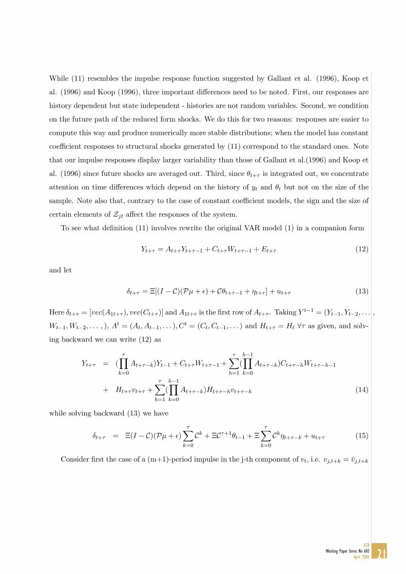
While (11) resembles the impulse response function suggested by Gallant et al. (1996), Koop et

al. (1996) and Koop (1996), three important differences need to be noted. First, our responses are

history dependent but state independent - histories are not random variables. Second, we condition

on the future path of the reduced form shocks. We do this for two reasons: responses are easier to

compute this way and produce numerically more stable distributions; when the model has constant

coefficient responses to structural shocks generated by (11) correspond to the standard ones. Note

that our impulse responses display larger variability than those of Gallant et al.(1996) and Koop et

al. (1996) since future shocks are averaged out. Third, since θt+τ is integrated out, we concentrate

attention on time differences which depend on the history of yt and θt but not on the size of the

sample. Note also that, contrary to the case of constant coefficient models, the sign and the size of

certain elements of Zjt affect the responses of the system.

To see what definition (11) involves rewrite the original VAR model (1) in a companion form

Yt+τ = At+τYt+τ−1 + Ct+τWt+τ−1 +Et+τ (12)

and let

δt+τ = Ξ[(I − C)(Pµ+ ) + Cθt+τ−1 + ηt+τ ] + ut+τ (13)

Here δt+τ = [vec(A1t+τ ), vec(Ct+τ )] andA1t+τ is the first row ofAt+τ . Taking Yt−1 = (Yt−1, Yt−2, . . . ,

Wt−1,Wt−2, . . . , ), At = (At, At−1, . . . ), Ct = (Ct, Ct−1, . . . ) and Ht+τ = Ht ∀τ as given, and solv-

ing backward we can write (12) as

Yt+τ = (τY

k=0

At+τ−k)Yt−1 + Ct+τWt+τ−1 +τX

h=1

(h−1Yk=0

At+τ−k)Ct+τ−hWt+τ−h−1

+ Ht+τvt+τ +τX

h=1

(h−1Yk=0

At+τ−k)Ht+τ−hvt+τ−h (14)

while solving backward (13) we have

δt+τ = Ξ(I − C)(Pµ+ )τX

k=0

Ck + ΞCτ+1θt−1 + ΞτX

k=0

Ckηt+τ−k + ut+τ (15)

Consider first the case of a (m+1)-period impulse in the j-th component of vt, i.e. vj,t+k = vj,t+k

21ECB


while v−j,t+k, k = 0, 1, . . . ,m and vt+m0 ∀m0 > m are unrestricted. Then

IR(t, t+ τ) = Et[Yt+τ |Y t−1, δt,Vt,Ht, vjt+mmk=0, v−jt+kmk=0, vt+kτk=m+1]

− Et[Yt+τ |Y t−1, δt,Vt,Ht, vt+kτk=0]

= Et[(τ−1Yk=0

At+τ−k)jHj

t (vjt −Evjt) + (τ−2Yk=0

At+τ−k)jHj

t+1(vjt+1 −Evjt+1) + . . .

+ (τ−m−1Yk=0

At+τ−k)jHj

t+m(vjt+m −Evjt+m)] (16)

where the superscript j refers to the j-th column of the matrix. It is easy to see that, when δt = δ,∀t,

(16) reduces to standard impulse responses and that when Et and ηt are correlated, both the sign

and the size of the shocks matter since, e.g. a shock in vt induces changes in δt.

Given (16), responses in our reparametrized model can be computed as follows

1. Choose a t, a τ and an Jt. Draw Ωl = H l

t(Hlt)02)l, (Bt)

l,Ψl from their posterior distribution

and ult from N(0, (σ2)lI ⊗H lt(H

lt)0). Compute ylt = Xtθt +Htvt +Xtu

lt.

2. Use the law of motion of the coefficients to compute θlt+1, l = 1, . . . , L after drawing

ηlt+1, ult+1,

l and the definition of Ξ to compute Xt+1. Draw ult+1 from N(0, (σ2)lI⊗H lt(H

lt)0)

and compute ylt+1 = Xt+1θlt+1 +Htvt+1 +Xt+1ult+1, l = 1, . . . , L.

3. Repeat step 2. and compute θlt+k, ylt+k, k = 2, . . . τ .

4. Repeat steps 1.-3. setting vt+k = E(vt+k), k = 0, . . . ,m using the draws for the shocks in

1.-3.

Shocks to the law of motion of the factors can be computed in the same way. A shock in ηt = η

lasting one period implies from (15) that

E(δt+τ − δt+τ ) = ΞmXk=0

Ht+kCk(ηt+τ−k −Eηt+τ−k) (17)

so that

IR(t, t+ τ) = Et[τY

k=0

(At+1τ−k −At+τ−k)Yt−1 +τX

h=1

h−1Yk=0

(At+1τ−k −At+τ−k)Ct+τ−hWt+τ−h−1(18)

+τX

h=1

h−1Yk=0

(At+1τ−k −At+τ−k)Ht+τ−hvt+τ−h] (19)

Therefore, responses to shocks in the factors can also be easily computed using the output of the

Gibbs sampler routine.


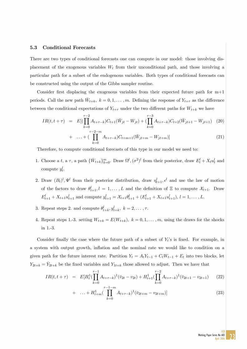
5.3 Conditional Forecasts

There are two types of conditional forecasts one can compute in our model: those involving dis-

placement of the exogenous variables Wt from their unconditional path, and those involving a

particular path for a subset of the endogenous variables. Both types of conditional forecasts can

be constructed using the output of the Gibbs sampler routine.

Consider first displacing the exogenous variables from their expected future path for m+1

periods. Call the new path Wt+k, k = 0, 1, . . . ,m. Defining the response of Yt+τ as the difference

between the conditional expectations of Yt+τ under the two different paths for Wt+k we have

IR(t, t+ τ) = E[(τ−2Yk=0

At+τ−k)Ct+1(Wjt −Wjt) + (τ−3Yk=0

At+τ−k)Ct+2(Wjt+1 −Wjt+1) (20)

+ . . .+ (τ−2−mYk=0

At+τ−k)Ct+m+1(Wjt+m −Wjt+m)] (21)

Therefore, to compute conditional forecasts of this type in our model we need to:

1. Choose a t, a τ , a path Wt+kmk=0. Draw Ωl, (σ2)l from their posterior, draw Elt +Xtu

lt and

compute ylt.

2. Draw (Bt)l,Ψl from their posterior distribution, draw ηlt+1,

l and use the law of motion

of the factors to draw θlt+1, l = 1, . . . , L and the definition of Ξ to compute Xt+1. Draw

Elt+1 +Xt+1u

lt+1 and compute y

lt+1 = Xt+1θlt+1 + (El

t+1 +Xt+1ult+1), l = 1, . . . , L.

3. Repeat steps 2. and compute θlt+k, ylt+k, k = 2, . . . , τ .

4. Repeat steps 1.-3. setting Wt+k = E(Wt+k), k = 0, 1, . . . ,m, using the draws for the shocks

in 1.-3.

Consider finally the case where the future path of a subset of Yt’s is fixed. For example, in

a system with output growth, inflation and the nominal rate we would like to condition on a

given path for the future interest rate. Partition Yt = AtYt−1 + CtWt−1 + Et into two blocks, let

Y2t+k = Y2t+k be the fixed variables and Y1t+k those allowed to adjust. Then we have that

IR(t, t+ τ) = E[H1t (

τ−1Yk=0

At+τ−k)1(v2t − v2t) +H1

t+1(τ−2Yk=0

At+τ−k)1(v2t+1 − v2t+1) (22)

+ . . .+H1t+m(

τ−1−mYk=0

At+τ−k)1(v2t+m − v2t+m)] (23)

23ECB


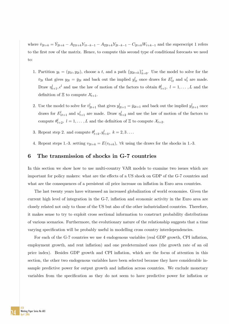
where v2t+k = Y2t+k −A21t+kY1t−k−1 −A22t+kY2t−k−1 − C2t+kWt+k−1 and the superscript 1 refers

to the first row of the matrix. Hence, to compute this second type of conditional forecasts we need

to:

1. Partition yt = (y1t, y2t), choose a t, and a path y2t+kτk=0. Use the model to solve for the

v2t that gives y2t = y2t and back out the implied yl1t once draws for El1t and ult are made.

Draw ηlt+1,l and use the law of motion of the factors to obtain θlt+1, l = 1, . . . , L and the

definition of Ξ to compute Xt+1.

2. Use the model to solve for vl2t+1 that gives yl2t+1 = y2t+1 and back out the implied y

l1t+1 once

draws for El1t+1 and ult+1 are made. Draw ηlt+2 and use the law of motion of the factors to

compute θlt+2, l = 1, . . . , L and the definition of Ξ to compute Xt+2.

3. Repeat step 2. and compute θlt+k, ylt+k, k = 2, 3 . . . .

4. Repeat steps 1.-3. setting v2t+k = E(vt+k), ∀k using the draws for the shocks in 1.-3.

6 The transmission of shocks in G-7 countries

In this section we show how to use multi-country VAR models to examine two issues which are

important for policy makers: what are the effects of a US shock on GDP of the G-7 countries and

what are the consequences of a persistent oil price increase on inflation in Euro area countries.

The last twenty years have witnessed an increased globalization of world economies. Given the

current high level of integration in the G-7, inflation and economic activity in the Euro area are

closely related not only to those of the US but also of the other industrialized countries. Therefore,

it makes sense to try to exploit cross sectional information to construct probability distributions

of various scenarios. Furthermore, the evolutionary nature of the relationship suggests that a time

varying specification will be probably useful in modelling cross country interdependencies.

For each of the G-7 countries we use 4 endogenous variables (real GDP growth, CPI inflation,

employment growth, and rent inflation) and one predetermined ones (the growth rate of an oil

price index). Besides GDP growth and CPI inflation, which are the focus of attention in this

section, the other two endogenous variables have been selected because they have considerable in-

sample predictive power for output growth and inflation across countries. We exclude monetary

variables from the specification as they do not seem to have predictive power for inflation or


output growth once lags of these variables are included. Five lags of the endogenous variables,

a constant and two lags of the predetermined variable are used. Therefore, each equation has

k=7*4*5+2=1=143 coefficients and there are 28 equations in the system. The estimation sample

covers the period 1980:1-2000:4, and the exercises we conduct are conditional on estimates obtained

with the information up to 2000:4. Since a training sample is not available, we set Ψ = C = 0,

P = I, a = 10, b = 1, choose ζt = 1 , B = bi ∗ I and let p(bi) = G(0.5, 5), i = 1, 2, . . . , F . We

initialize θ with a sequential OLS on the time invariant version of the model and set σ2 to the

average estimated variances of NG AR(p) models.

The vector δt is decomposed into three factors: a 2× 1 vector of common factors, θ1t - one for

the Euro area and one for the rest of the world; a 7× 1 vector of country specific factors, θ2t; and

a 4× 1 vector of variable specific factors, θ3t, Hence, θt = (θ01t, θ02t, θ03t)0 is 13× 1 vector.

We produce 55,000 iterations of the MCMC routine starting from arbitrary initial conditions.

Runs of 50 elements are drawn 1100 times and the last observation of the final 1000 runs was used

for inference. We checked convergence recursively calculating the first two moments of the posterior

of the parameters using 300, 500, 1000 draws and found that convergence was sufficiently easy to

achieve and obtained with about 500 draws.

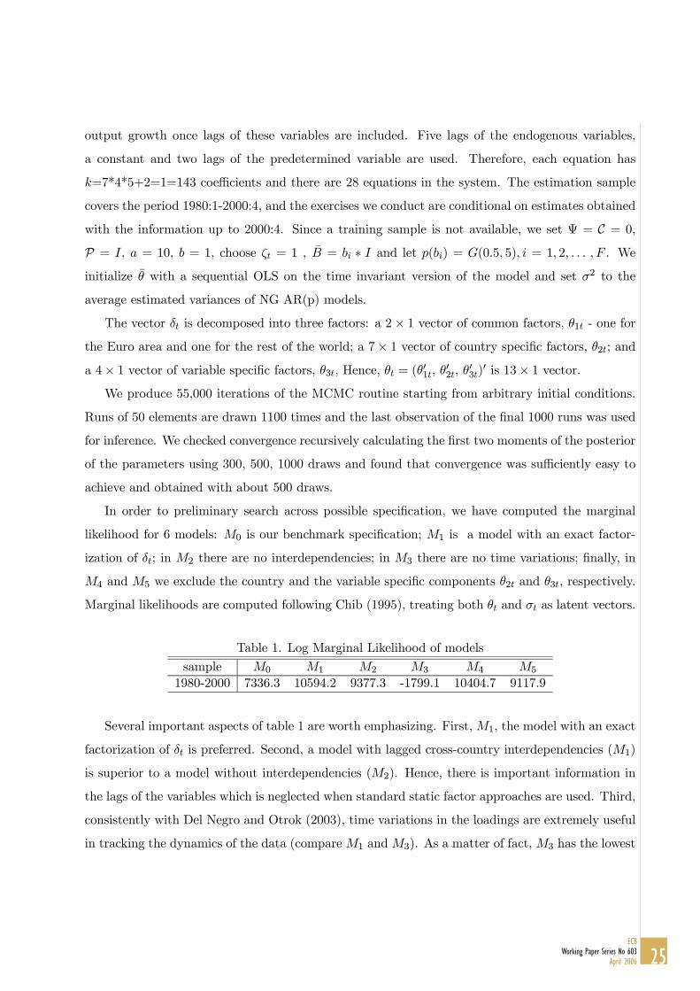
In order to preliminary search across possible specification, we have computed the marginal

likelihood for 6 models: M0 is our benchmark specification; M1 is a model with an exact factor-

ization of δt; in M2 there are no interdependencies; in M3 there are no time variations; finally, in

M4 and M5 we exclude the country and the variable specific components θ2t and θ3t, respectively.

Marginal likelihoods are computed following Chib (1995), treating both θt and σt as latent vectors.

Table 1. Log Marginal Likelihood of models

sample M0 M1 M2 M3 M4 M5

1980-2000 7336.3 10594.2 9377.3 -1799.1 10404.7 9117.9

Several important aspects of table 1 are worth emphasizing. First,M1, the model with an exact

factorization of δt is preferred. Second, a model with lagged cross-country interdependencies (M1)

is superior to a model without interdependencies (M2). Hence, there is important information in

the lags of the variables which is neglected when standard static factor approaches are used. Third,

consistently with Del Negro and Otrok (2003), time variations in the loadings are extremely useful

in tracking the dynamics of the data (compareM1 andM3). As a matter of fact,M3 has the lowest

25ECB


marginal likelihood of all the specifications we consider. Finally the marginal likelihood of a model

with three indices is always higher than the marginal likelihood of a model with only two indices,

regardless of whether the two indices capture world and variable specific factors (M4), or world and

country specific factors (M5).

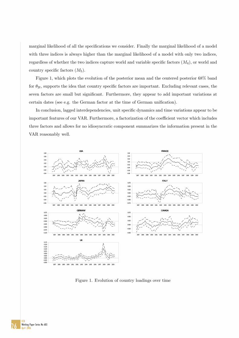
Figure 1, which plots the evolution of the posterior mean and the centered posterior 68% band

for θ2t, supports the idea that country specific factors are important. Excluding relevant cases, the

seven factors are small but significant. Furthermore, they appear to add important variations at

certain dates (see e.g. the German factor at the time of German unification).

In conclusion, lagged interdependencies, unit specific dynamics and time variations appear to be

important features of our VAR. Furthermore, a factorization of the coefficient vector which includes

three factors and allows for no idiosyncratic component summarizes the information present in the

VAR reasonably well.

USA

1987 1988 1989 1990 1991 1992 1993 1994 1995 1996 1997 1998 1999 2000-0.04

-0.02

0.00

0.02

0.04

0.06

0.08

JAPAN

1987 1988 1989 1990 1991 1992 1993 1994 1995 1996 1997 1998 1999 2000-0.06

-0.04

-0.02

0.00

0.02

0.04

0.06

GERMANY

1987 1988 1989 1990 1991 1992 1993 1994 1995 1996 1997 1998 1999 2000-0.100

-0.075

-0.050

-0.025

-0.000

0.025

0.050

0.075

UK

1987 1988 1989 1990 1991 1992 1993 1994 1995 1996 1997 1998 1999 2000-0.050-0.0250.0000.0250.0500.0750.1000.1250.1500.175

FRANCE

1987 1988 1989 1990 1991 1992 1993 1994 1995 1996 1997 1998 1999 2000-0.08

-0.06

-0.04

-0.02

0.00

0.02

0.04

0.06

ITALY

1987 1988 1989 1990 1991 1992 1993 1994 1995 1996 1997 1998 1999 2000-0.075

-0.050

-0.025

0.000

0.025

0.050

0.075

CANADA

1987 1988 1989 1990 1991 1992 1993 1994 1995 1996 1997 1998 1999 2000-0.050

-0.025

0.000

0.025

0.050

0.075

Figure 1. Evolution of country loadings over time


First, we consider the effect of a US real shocks on the GDP of other countries. We con-

struct such a shock by making US variables contemporaneously casually prior. Within the US

block, employment growth and output growth increase by one unit for one period, while the other

two variables change according to the domestic correlation matrix. Figure 2 presents the median

responses together with a 68 percent posterior band. Three features of the figure are worth empha-

sizing. First, responses are relatively smooth despite the large number of VAR parameters because

of the moving average nature of our indices. Second, there appears to be a significant Anglo-Saxon

real cycle with Canadian and UK GDP growth responding significantly and instantaneously to

the US shock. The response is instantaneously significant also in Japan and, to a much smaller

extent, in Germany. Third, the peak response in Italy and France is delayed by at least one period,

suggesting that transmission to these two countries takes time an probably occurs via Germany.

Finally, impulses typically dissipate very quickly: except for Italy and France, all response bands

include zero two quarters after the shocks.

-1,5

-1,0

-0,5

0,0

0,5

1,0

1,5

2,0

1 3 5 7 9 11 13 15 17 19 21

Japan

-1,5

-1,0

-0,5

0,0

0,5

1,0

1,5

2,0

1 3 5 7 9 11 13 15 17 19 21

UK

-1,5

-1,0

-0,5

0,0

0,5

1,0

1,5

2,0

1 3 5 7 9 11 13 15 17 19 21

Canada

-1,5

-1,0

-0,5

0,0

0,5

1,0

1,5

2,0

1 3 5 7 9 11 13 15 17 19 21

Germany

-1,5

-1,0

-0,5

0,0

0,5

1,0

1,5

2,0

1 3 5 7 9 11 13 15 17 19 21

France

-1,5

-1,0

-0,5

0,0

0,5

1,0

1,5

2,0

1 3 5 7 9 11 13 15 17 19 21

Italy

Figure 2. Responses of GDP growth to a shock to the growth rate of real US variables

Next, we consider the response of inflation in the three European countries when the growth

rate of the oil price index is 30 percent higher than its 2000:4 level and the increase lasts for four

27ECB


quarters. Figure 3 reports the posterior median and the posterior 68% band for inflation responses

in Germany, Italy and France. Responses in the three countries look different in magnitude and

timing. All countries have a delayed peak reaction. However, the peak of German inflation occurs

after 3 to 4 quarters after the shock has died out, whereas for Italy and France the peak response

is at quarter 2 and the reaction remains significantly positive only for 3 to 4 quarters, roughly the

length of the increase. Interestingly, the average magnitude of the reaction of French inflation is

lower than the one obtained in Italy and Germany.

-5.0

0.0

5.0

10.0

15.0

20.0

1 2 3 4 5 6 7 8 9 10 11 12 13

Germany

-5.0

0.0

5.0

10.0

15.0

20.0

1 2 3 4 5 6 7 8 9 10 11 12 13

France

-5.0

0.0

5.0

10.0

15.0

20.0

1 2 3 4 5 6 7 8 9 10 11 12 13

Italy

Figure 3. Responses of inflation to an oil price growth shock

Finally, the estimated model can be used to compute a variety of measures which are of interest

for policymakers. In Figure 4 we present the time profile for the posterior 68% band for a coinci-

dent measure of potential world output growth, constructed as CV LIGDPt = (X1tθ1t + X3tθ3t)GDP .

Three features are worth emphasizing. First, cyclical movements of potential output roughly cor-

respond to those of actual output. Second, there is a marked and significant difference in the level

of potential output growth in the 1990’s as compared to the end of 1980’s. The decline is driven by

both Japanese and the Euro area variables. Third, our measure of potential output starts declining

significantly at the beginning of 2000.


1987 1989 1991 1993 1995 1997 1999-4

-2

0

2

4

6

8

Figure 4. Potential output growth

7 Conclusions

This paper develops an approach to conduct inference in time varying coefficient multi-country VAR

models with lagged cross unit interdependencies and unit specific dynamics. We take a Bayesian

viewpoint to estimation and restrict the coefficients to have a low dimensional time varying factor

structure. We complete the specifications using a hierarchical prior for the vector of factors which

allows for exchangeability, time variations and heteroschedasticity in the innovations in the factors.

The factor structure on the coefficients allows us to transform an overparametrized VAR into

a parsimonious SUR model where the regressors are observable linear combinations of the right-

hand-side variables of the VAR, and the loadings are the time varying coefficient factors. We

derive posterior distributions for the vector of loadings using Markov Chain Monte Carlo methods.

We show how to construct unconditional forecasts, responses to impulses in interesting structural

shocks and conditional forecasts, using the output of the MCMC routine.

The reparametrization of the VAR has a number of appealing features. First, it reduces the

problem of estimating a large number of, possibly, unit specific and time varying coefficients into

the problem of estimating a small number of loadings on certain combinations of the right hand

side variables of the VAR. Second, since the regressors of the model are observable, the model can

be employed recursively for a variety of policy purposes. Third, since indices are predetermined

29ECB


with respect to the endogenous variables, it is easy to construct Bayes factors to select the number

of indices or to examine the model specification to be used.

The tools described in this paper can be applied to a number of interesting problems. For ex-

ample, Canova, et al. (2003) have used a multi-country VAR to extract world and national business

cycles while Anzuini, et al. (2005) use a multi-country VAR structure to construct coincident and

leading indicators for inflation and output growth in Italy and the Euro area. The construction of

measures of core inflation and of the natural rate of unemployment in multi-country settings, the

study of the transmission of monetary policy shocks across economic areas and sectors, and the

construction of portfolios of assets in different geographical regions can all be studied within the

general framework presented in this paper.

To conclude, one should mention that the procedure is far from being computationally demand-

ing (one full run of the MCMC routine for the example of section 6 takes about 45 minutes).

Therefore, the approach is at least competitive with existing alternatives.


References

[1] Anzuini, A. Caivano, M., Canova, F., Lamorgese, A. and Venditti, F. (2005), A leading

indicator for Inflation and GDP growth in Italy and the Euro area, Bank of Italy, manuscript.

[2] Binder, M., C. Hsiao and H. Pesaran (2001), Estimation and Inference in Short Panel Vector

Autoregressions with Unit Roots and Cointegration, University of Maryland, manuscript.

[3] Canova, F. (1993), Modelling and Forecasting Exchange Rates using a Bayesian Time varying

coefficient model, Journal of Economic Dynamics and Control, 17, 233-262.

[4] Canova, F. and M. Ciccarelli (2004), Forecasting and Turning Point Prediction in a Bayesian

Panel VAR Model, Journal of Econometrics, 120, 327-359.

[5] Canova, F., M. Ciccarelli and E. Ortega (2003), Similarities and Convergence of G-7 cycles,

forthcoming, Journal of Monetary Economics.

[6] Canova, F. and Pappa, E. (2003), Price differential in monetary unions: the role of fiscal

shocks, forthcoming, Economic Journal.

[7] Ciccarelli, M and Rebucci, A. (2003) Measuring Contagion using a Bayesian Time varying

coefficient model, ECB Working paper.

[8] Chamberlin, G. (1983), Panel Data, in Griliches, Z. and M. Intrilligator (eds.), The Handbook

of Econometrics, II, North Holland.

[9] Chib, S. (1995), Marginal Likelihood from the Gibbs output, Journal of the American Statis-

tical Association, 90, 1313-1321.

[10] Chib, S. and E. Greenberg (1995), Hierarchical Analysis of SUR Models with Extensions to

Correlated Serial Errors and Time-Varying Parameter Models, Journal of Econometrics, 68,

409—431.

[11] Cogley, T. and T. Sargent (2005), Drift and Volatilities: Monetary Policy and Output in Post

WWII US, Stanford University, Review of Economic Dynamics,8, 275-308.

[12] Forni, M., M. Hallin, M. Lippi and L. Reichlin (2000), The Generalized Dynamic-Factor

Model: identification and estimation, The Review of Economics and Statistics, 82(4) 540-54.

31ECB


[13] Del Negro, M. and Otrok, C. (2003) Dynamic Factor Models with Time-Varying Parameters:

Measuring the evolution of the European Business Cycle, Federal Reserve Bank of Atlanta,

manuscript.

[14] Doan, T., R. Litterman and C. Sims (1984), Forecasting and Conditional Projection using

Realistic Prior Distributions, Econometric Reviews,3, 1-100.

[15] Gallant, R., P. Rossi and G. Tauchen (1993), Nonlinear Dynamic Structures, Econometrica,

61, 871-907.

[16] Gelfand, A. and Dey, D. (1994) Bayesian Model Choice: Asymptotics and Exact Calculations,

Journal of the Royal Statistical Society, Ser B, 56, 501-514.

[17] Geweke, J. (2000) Simulation Based Bayesian Inference for Economic Time Series, in Mariano,

R., Shuermann and M. Weeks (eds.) Simulation Based Inference in Econometrics: Methods

and Applications, Cambridge, Cambridge University Press.

[18] Holtz—Eakin D., W. Newey and H. Rosen (1988), Estimating vector autoregressions with

panel data, Econometrica, 56(6), 1371—1395.

[19] Hsiao, C., M.H. Pesaran and A.K. Tahmiscioglu (1999), Bayes estimation of short run co-

efficients in dynamic panel data models, in Hsiao et al. (eds.) Analysis of panels and limited

dependent variable models: in honor of G.S. Maddala, Cambridge, Cambridge University

Press.

[20] Kadiyala, R. and S. Karlsson (1997), Numerical Methods for Estimation and Inference in

Bayesian VAR models, Journal of Applied Econometrics, 12, 99-132.

[21] Kass, R. and Ratfery, A. (1995), Bayes Factors, Journal of the American Statistical Associa-

tion, 90, 773-795.

[22] Kim, and Nelson, C. (1998) Business Cycle Turning Points, a New Coincident Index and tests

of Duration Dependence based on a Dynamic Factor Model with Regime Switching, Review of

Economics and Statistics, 80(3), 188-201.

[23] Koop, G., H. Pesaran and S. Potter (1996), Impulse Response Analysis in non-linear Multi-

variate Models, Journal of Econometrics, 74, 119-147.


[24] Imbs, J., Mumtaz, H., Ravn, M. and Rey, H. (2005), PPP strikes back: Aggregation and the

Real Exchange Rate, Quarterly Journal of Economics, CXX,1-43.

[25] Pesaran, H. (2003), Estimation and Inference in Large Heterogeneous Panels with Cross

Section Dependence, University of Cambridge, working paper 0305.

[26] Pesaran, H. and R. Smith (1996), Estimating Long Run Relationships for Dynamic Heteroge-

nous Panels, Journal of Econometrics, 68, 79-113.

[27] Stock, J. and M. Watson (1999), Diffusion Indices, Harvard University, manuscript.

33ECB


European Central Bank Working Paper Series

For a complete list of Working Papers published by the ECB, please visit the ECB’s website(http://www.ecb.int)

570 “Household debt sustainability: what explains household non-performing loans? An empiricalanalysis” by L. Rinaldi and A. Sanchis-Arellano, January 2006.

571 “Are emerging market currency crises predictable? A test” by T. A. Peltonen, January 2006.

572 “Information, habits, and consumption behavior: evidence from micro data” by M. Kuismanenand L. Pistaferri, January 2006.

573 “Credit chains and the propagation of financial distress” by F. Boissay, January 2006.

574 “Inflation convergence and divergence within the European Monetary Union” by F. Busetti,L. Forni, A. Harvey and F. Venditti, January 2006.

575 “Growth in euro area labour quality” by G. Schwerdt and J. Turunen, January 2006.

576 “Debt stabilizing fiscal rules” by P. Michel, L. von Thadden and J.-P. Vidal, January 2006.

577 “Distortionary taxation, debt, and the price level” by A. Schabert and L. von Thadden,January 2006.

578 “Forecasting ECB monetary policy: accuracy is (still) a matter of geography” by H. Berger,M. Ehrmann and M. Fratzscher, January 2006.

579 “A disaggregated framework for the analysis of structural developments in public finances”by J. Kremer, C. Rodrigues Braz, T. Brosens, G. Langenus, S. Momigliano and M. Spolander,January 2006.

580 ”Bank interest rate pass-through in the euro area: a cross country comparison”by C. K. Sørensen and T. Werner, January 2006.

581 “Public sector efficiency for new EU Member States and emerging markets” by A. Afonso,L. Schuknecht and V. Tanzi, January 2006.

582 “What accounts for the changes in U.S. fiscal policy transmission?” by F. O. Bilbiie, A. Meierand G. J. Müller, January 2006.

583 “Back to square one: identification issues in DSGE models” by F. Canova and L. Sala,January 2006.

584 “A new theory of forecasting” by S. Manganelli, January 2006.

585 “Are specific skills an obstacle to labor market adjustment? Theory and an application to the EUenlargement” by A. Lamo, J. Messina and E. Wasmer, February 2006.

586 “A method to generate structural impulse-responses for measuring the effects of shocks instructural macro models” by A. Beyer and R. E. A. Farmer, February 2006.


587 “Determinants of business cycle synchronisation across euro area countries” by U. Böwer andC. Guillemineau, February 2006.

588 “Rational inattention, inflation developments and perceptions after the euro cash changeover”by M. Ehrmann, February 2006.

589 “Forecasting economic aggregates by disaggregates” by D. F. Hendry and K. Hubrich,February 2006.

590 “The pecking order of cross-border investment” by C. Daude and M. Fratzscher, February 2006.

591 “Cointegration in panel data with breaks and cross-section dependence” by A. Banerjee andJ. L. Carrion-i-Silvestre, February 2006.

592 “Non-linear dynamics in the euro area demand for M1” by A. Calza and A. Zaghini,February 2006.

593 “Robustifying learnability” by R. J. Tetlow and P. von zur Muehlen, February 2006.

594

595 “Trends and cycles in the euro area: how much heterogeneity and should we worry about it?”by D. Giannone and L. Reichlin, comments by B. E. Sørensen and M. McCarthy, March 2006.

596 “The effects of EMU on structural reforms in labour and product markets” by R. Duvaland J. Elmeskov, comments by S. Nickell and J. F. Jimeno, March 2006.

597 “Price setting and inflation persistence: did EMU matter?” by I. Angeloni, L. Aucremanne,M. Ciccarelli, comments by W. T. Dickens and T. Yates, March 2006.

598 “The impact of the euro on financial markets” by L. Cappiello, P. Hördahl, A. Kadarejaand S. Manganelli, comments by X. Vives and B. Gerard, March 2006.

599 “What effects is EMU having on the euro area and its Member Countries? An overview”by F. P. Mongelli and J. L. Vega, March 2006.

600 “A speed limit monetary policy rule for the euro area” by L. Stracca, April 2006.

601 “Excess burden and the cost of inefficiency in public services provision” by A. Afonsoand V. Gaspar, April 2006.

602 “Job flow dynamics and firing restrictions: evidence from Europe” by J. Messina and G. Vallanti,April 2006.

603 “Estimating multi-country VAR models” by F. Canova and M. Ciccarelli, April 2006.

35ECB


“The euro’s trade effects” by R. Baldwin, comments by J. A. Frankel and J. Melitz, March 2006.

ISSN 1561081-0

9 7 7 1 5 6 1 0 8 1 0 0 5

Estimating multi-country VAR models - European Central Bank

Documents

Transcript of Estimating multi-country VAR models - European Central Bank