1

Estimating insurer´s capital requirements through Markov

switching models in the Solvency II framework

L. Oteroa,*, P. Durán

b, S. Fernández

c and M. Vivel

d.

a,b,c,d Department of Finance and Accounting, University of Santiago of

Compostela, Santiago of Compostela (Spain).

*Corresponding author. E-mail: luis.otero@usc.es

ABSTRACT: Solvency II will transform the system for determining capital requirements

for insurers. The new regulatory framework proposes a standard model, but at the same

time, it encourages the use of internal models of self-evaluation and risk management.

This paper attempts to assess the adequacy of Markov switching models for the design of

internal models of insurers' equity risk exposure. We have used monthly data from four of

the main European indices for the period between January1990 and January 2010. The

comparison of models across different statistical criteria and backtesting shows the

superiority of Markov switching models over simpler models, to capture insurers' equity

risk. Subsequently, we compared capital requirements resulting from applying these

models against the Solvency II proposal. The results showed that the funds needed to take

the equity risk are dependent on the specification used. Also, the capital raised by Markov

switching specifications exceeds those of the standard model. This means that companies

using the standard model or another based on similar assumptions are underestimating the

risk actually assumed.

2

I. Introduction

The new UE solvency regulation, known as Solvency II, involves the revision of

standards for evaluating the financial condition of insurance companies. Under the new

framework, the determination of capital requirements can be done through a standard

model or internal models previously approved by the regulator. On 10 November 2009,

the ECOFIN (Council of Ministers of Economy and Finance of the European Union) has

adopted the new Directive, and, therefore, the transposition into national standards should

be carried out before the end of 2012. The standard model development was carried out

through a total of five quantitative impact studies (QIS) conducted by the Committee of

European Insurance Supervisors (CEIOPS). The new legislation promotes the use of

alternative internal models for managing risk and determining capital requirements.

Equity risk is included within the market risk module and, under the new Solvency II

Directive (Commission of the European Communities, 2009), measures the sensitivity of

the value of assets, liabilities and financial instruments to changes in the level or volatility

of market share prices. This risk is the main component of the investment portfolios of

European insurers, accounting for 34.3% in 2007. The model of normal returns implicit in

the calculation of the standard formula has been chosen for simplicity. However, the

normality assumption may underestimate the tail of the distribution of losses and not

capture the variations in volatility possibly variability, making it less suitable to represent

longer periods of time (Hardy, 2001). The returns may have other properties such as

serial autocorrelation in the mean, volatility not constant over time (heteroscedasticity)

and clusters of volatility. Autoregressive models AR (p) and ARMA are adequate to

capture the serial dependence that exists among the asset returns. In addition, the variance

may vary over time, in which case the ARCH and GARCH models may be appropriate as

conditional variance modeled itself on the basis of past values of the variable itself (Engle

1982, Bollerslev, 1986). In subsequent proposals, the models been have adapted to

incorporate the so-called leverage effect among which are the exponential GARCH or

3

EGARCH (Nelson, 1991) and the GJR-GARCH (Glosten et al. 1993). However, the

models mentioned above are not able to capture sudden changes in market behavior that

happen in crisis situations or to sudden changes in government policy. The transformation

of the previous models introducing regime switching may be better suited to measuring

the risk of equity. In this sense, some studies have shown the superiority of these models

for series of short-term yields (Li and Lin, 2004, Maekawa et al., 2005; Rapach and

Strauss, 2005; and Sajjad, Coakley and Nankervis, 2008). However, in the framework of

Solvency II, market risk is determined by the VaR at 99.5% within one year. For this

reason, some studies have evaluated the adequacy of the models using other periods of

analysis (Hardy (2001), Won and Chang (2005) and Hardy et al. (2006)).

This paper analyzes the suitability of Markov regime-switching for building internal

models of equity risk. Thus, we analyze their ability to capture the dramatic changes

observed in the behavior of markets. Several models have been calibrated to the monthly

series of major European indices and then compared using different criteria.

Subsequently, Monte Carlo simulation has been carried out to calculate capital

requirements under the specifications of Solvency II. This study contributes to existing

literature providing a new approach that has not yet been applied to the European market.

Furthermore, unlike previous studies, we have included a variety of regime switching

models and the selection has been done through the implementation of backtesting and

not based solely on statistical criteria. The results could be very useful for the calibration

of the standard model and, also, for insurance companies wishing to opt for an internal

model.

The paper is structured as follows. In section 2 we review the previous literature.

Subsequently, section 3 outlines the models that will be analyzed. Section 4 discusses the

series of indices used in the empirical analysis. Section 5 presents the estimation and

evaluation of models, and section 6 makes a comparative analysis of the results of

4

applying the proposed models for determining capital requirements. Finally, conclusions

are presented.

II. Theoretical Framework

The evaluation of equity risk models must take into account the particularities of this type

of exposition in the case of insurance companies. This is very important because the

models that best project the behavior of short term returns may not be the most suitable

for analyzing long term risk. In this sense, most studies have shown the superiority of

different specifications of regime switching models, but using series of short term yields

(Li and Lin, 2004, Maekawa et al., 2005; Rapach and Strauss, 2005; and Sajjad, Coakley

and Nankervis, 2008). However, a number of authors have focused on long term risk

analysis for insurers evaluating several basic RS models using monthly returns and

obtained similar results. Thus, Hardy (2001) evaluated the suitability of different models,

concluding that the Regime Switching Lognormal Model provides a better fit than the

other models tested. Bayliff and Pauling (2003) conducted a comparison of the lognormal

model, lognormal autoregressive, GARCH and RSLN, and concluded that the models that

have mean reversion and fat tails are the ones that provide the best fit for long-term data.

Wong and Chan (2005) employed two new models, the mixture autoregressive (MAR)

and the mixture of ARCH (MARCH), for monthly returns of the TSE 300 and S&P 500.

The results of this paper show that new models fit worse than the regime switching

(RSLN) alternative, although they may be useful for modeling tails. A similar study was

performed by Hardy et al. (2006) who compared a large number of models estimated by

maximum likelihood for the return of the S&P-500, reaching the conclusion that regimen

switching has the best fit in the left tail of the distribution and, therefore, is more suitable

for risk assessment. Finally, Boudreault and Panneton (2009) conducted a comparison of

different multivariate models for monthly returns in Canadian, American, British and

Japanese markets. In general, it appears that GARCH models have a better adjustment

5

than regime switching, but the latter represent the thick tails of the distribution much

better.

3. Models Considered for Equity Risk Assessment.

Table 2 lists the specifications of the models that have been evaluated for consideration as

alternatives to incorporate into an internal model. In particular, we have considered the

lognormal model, because it is implicit in the Solvency II standard framework, GARCH

and EGARCH models and their variants of regime switching. Thus we try to evaluate if

the addition of regime switching is suitable for modeling the long term risk of equity.

Models description

Regimen switching lognormal model (RSL()

Regime switching was introduced by Hamilton (1989), who described an

autoregressive regime switching process. In Hamilton and Susmel (1994) several regime-

switching models are analyzed, varying the number of regimes and the form of the model

within regimes. The regime-switching lognormal model was proposed for the purpose of

modeling long-term equity returns in Hardy (2001), with further discussion in Hardy

(2003). This model uses a Markov chain = 1,2 … . which represents the evolution of the state of the economy, which can be in two possible situations known as regimes. In

each of the regimes, returns follow a normal independent distribution where the

parameters are different for each regime , namely: = + ( = 1,2) (1)

Where: ~(0; 1); = 1,2, … ; and represents each of the regimes. Regimen switching GARCH

This model was described by Gray (1996) who proposes an alternative that combines the

main features of the GARCH model within a regime-switching framework. This was

6

subsequently modified by Klaassen (2002), and Marcucci (2005) compares a set of

GARCH, EGARCH and GJR-GARCH models within an MS-GARCH framework

(Gaussian, Student’s t and Generalized Error Distribution for innovations) in terms of

their ability to forecast S&P100 volatilities. The model analyzed is a RS-GARCH(1,1)

with two regimes and constant in the equation of the mean, i.e.:

= , + where = , (2) Unlike RSLN model, which assumes a constant volatility, in regimen switching GARCH

models volatility varies according to an ARMA process, so that the equation for the

variance for each regime is given by:

, = + ( ) + ! ( = 1,2) (3) Cai (1994) and Hamilton and Susmel (1994) argue that MS-Garch models are intractable

because the conditional variance depends on the entire past history of the data. Gray

(1996) proposes the possibility of constructing a measure that is not path dependent: = " ,( + , ) + (1 − " ,)( + , ) − (" , + (1 − " ,)) (4) Under this approach the conditional variance depends on the regime alone, and not on the

entire history of the process

Regimen Switching E-GARCH

The asymmetric behavior of stock volatility has been well described in the literature.

Nelson (1991) proposes the EGarch model to capture this asymmetry. Equity returns tend

to display more volatility in the case of a negative shock than after a positive shock of

equal magnitude. The equation for the variance for each regime is given by:

log ( , ) = + '() *+,-./0+,+,-1 ( − 22/4)5 + ! log( ) + 6 *+,-

./+,-1 , ( = 1,2) (5)

7

The logarithmic form for the conditional variance ensures positive values, avoiding the constraints of non negativity characteristics in the estimation of Garch models. As

Henry (2008) says, since 6 tipically has a negative sign, a negative innovation generates more volatility than a positive one of equal magnitude.

Models estimation

As Hardy et al. (2006) says, the estimation for this models can be problematic as the

likelihood surface has many local maxima, many of which are very close to the global

maximum. This means that many parameter sets are more or less equally valid under

maximum likelihood estimation, even though the outcome may look very different. Those

models assume that the regime switching are exogenous and there are fixed probability

for each regime changes, where the regime is the realization of a M-state Markov chain

(Hamilton, 2005):

Pr9:;<=: = , : = >, … . . ? = Pr9:;<=: = ? = " < (6)

The transition matrix P contains transition probabilities " <, giving the probability that state i will be followed by state j. The estimation of the parameters can be done

maximizing by numerical optimization the log-likelihood function:

@AB C(D1, … … … . , DE; F) = ∑ log );,( 1 ΘΩ−ttyf E (7)

In the case of two regimes the value of the conditional probability density of the return is:

∑∑=

−

=

−−ΘΩ=⋅⋅=ΘΩ

2

1

1

2

1

1,1 );,|();,(i

ttt

J

ijtitt jSyfpyf π

(8)

Where the probability that the observed regime at time t evolves according to the

following equation:

);,(

);,|(

1

1

2

1

1,

,ΘΩ

ΘΩ=⋅⋅

=

−

−

=

−∑

tt

ttt

J

ijti

tiyf

jSyfpπ

π

(9)

8

Table 1. Specification of the models used in the analysis

Model Specification 1

Normal = + GARCH (1,1) = + ; = ; = + + !

EGARCH (1,1) = + ; = ; log() = + H*+,-/+,-H + I *+,-/+,- + ! log( ) RSLN (> regímenes) = + ; (" = 1, … , >) RS-GARCH (1,1) = + ; = ,; , = + ( ) + ! ; ( = 1,2) RS-EGARCH (1,1)

= + ; = ,; log ( , ) = + JK) *+,-./0+,+,-1 K − 22/4)L + ! log( ) + 6 *+,-

./+,-1 , ( =1,2)

IV.- Empirical Analysis of The Series

The data analyzed to calibrate equity risk comprises monthly observations of four

of the main European stock market index returns (FTSE 100, CAC40, DAX and IBEX-

35). Because insurance companies must protect the interests of their policyholders in the

medium and long term, it is common to use this data frequency [see Hardy (2001),

Panneton (2003), Wong and Chan (2005), Hardy et al. (2006) or Boudreault and

Panneton (2009)], and even the CEIOPS has calibrated the solvency standard European

model on a quarterly basis. Descriptive statistics and the information relative to normality

(Jarque Bera Test), are shown in table 2.

Table 2. Descriptive statistics, autocorrelation and normatility test of the main Market Index

CAC FTSE IBEX DAX

Mean 0,0027 0,0033 0,0068 0,0061

Median 0,0123 0,0075 0,0100 0,0137

Maximum 0,1259 0,1088 0,2342 0,1937

Minimum -0,1923 -0,1395 -0,2340 -0,2933

Std,Dev, 0,0573 0,0428 0,0666 0,0638

Skewness -0,5326 -0,5756 -0,2675 -0,8101

Kurtosis 3,4354 3,6043 4,2821 5,4654

1 ~(0; 1): is a standardized noise, i.e., consisting of independent variables with zero mean and variance equal to 1. In this paper we have used a normal white noise, but we can use other asymmetric

distributions such as Student t or generalized error distribution (GED).

9

JBstatistic 13,1325 16,9036 17,3706 83,0442

Probability 0,0014 0,0002 0,0002 0,0000

Observations 238 240 216 229

As can be seen in the different indices (Table 2 and Fig. 1), the mean return is not

very important and the skewness is significant and negative, implying a possible leverage

effect in the data, and the kurtosis is significant higher than that of a Gaussian

distribution, indicating fat-tailed returns. This is consistent with the values found at

Jarque-Bera statistic, which rejects the hypothesis of normality in the yields behavior of

different indexes.

As shown in Fig.2, yields have clusters of volatility. This feature can be seen in

the figure of the square of the logarithmic returns. For this reason it is important to

determine which model best fits the behavior of the variance over time. The simple

autocorrelation function (ACF) and partial autocorrelation function (PACF), represented

in Fig. 3, of the squared returns show a strong dependence structure, which implies the

existence of dependence in the variance of monthly returns. This means that the models

not considering a constant volatility over time may be more appropriate for assessing

market risk.

10

Fig.1. Histogram of monthly logarithmic returns and time series plot

0

5

10

15

20

25

-0.20 -0.15 -0.10 -0.05 0.00 0.05 0.10

CAC

0

5

10

15

20

25

30

35

-0.10 -0.05 -0.00 0.05 0.10

FTSE

0

10

20

30

40

-0.2 -0.1 -0.0 0.1 0.2

IBEX

0

10

20

30

40

50

-0.3 -0.2 -0.1 -0.0 0.1 0.2

DAX

-.20

-.15

-.10

-.05

.00

.05

.10

.15

90 92 94 96 98 00 02 04 06 08

CAC

-.15

-.10

-.05

.00

.05

.10

.15

90 92 94 96 98 00 02 04 06 08

FTSE

-.3

-.2

-.1

.0

.1

.2

.3

92 94 96 98 00 02 04 06 08

IBEX

-.3

-.2

-.1

.0

.1

.2

92 94 96 98 00 02 04 06 08

DAX

11

Fig. 2.- Auto correlation function (ACF) and partial auto correlation function (PACF) plots of squared returns.

0 5 10 15 20

0.0

0.2

0.4

0.6

0.8

1.0

Lag

AC

F

CAC

5 10 15 20

-0.1

0-0

.05

0.0

00

.05

0.1

00

.15

0.2

0

Lag

PA

CF

CAC

0 5 10 15 20

0.0

0.2

0.4

0.6

0.8

1.0

Lag

AC

F

FTSE

5 10 15 20

-0.1

0-0

.05

0.0

00

.05

0.1

00.1

50

.20

Lag

PA

CF

FTSE

0 5 10 15 20

0.0

0.2

0.4

0.6

0.8

1.0

Lag

AC

F

IBEX

5 10 15 20

-0.1

0.0

0.1

0.2

Lag

PA

CF

IBEX

0 5 10 15 20

0.0

0.2

0.4

0.6

0.8

1.0

Lag

AC

F

DAX

5 10 15 20

-0.1

0-0

.05

0.0

00

.05

0.1

00

.15

Lag

PA

CF

DAX

12

V.- Models Estimation and Comparison

In this section we present the results of estimating the models from the analyzed series

and comparing them, using different statistical criteria. All the models have been estimated

using TSM, an Ox package Developed by James Davidson, and E-Views 6. Table 4 shows the

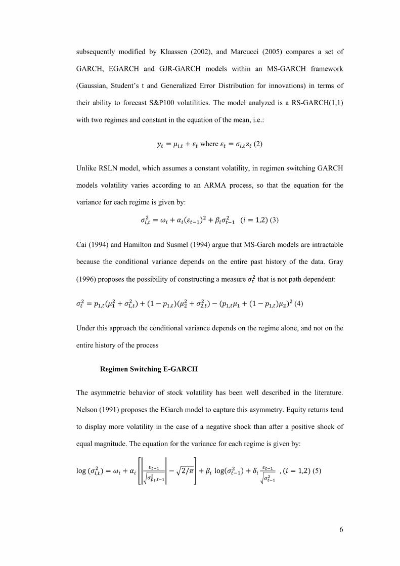
parameters resulting from the maximum likelihood estimation. The model of two regimes

(RSLN2), as is the case with the results obtained by Hardy (2001.2006) provides a more stable

regime with positive expected returns, and a more volatile one with a negative expected return.

The high significance of the parameters of the equation for the variance of the GARCH models

is consistent with the persistence of volatility in the empirical data. As can be seen, the

estimation of regime switching models involves a large number of parameters, and thus the

complexity of the estimation. In fact, E-GARCH Regime switching could not be estimated since

the algorithm presented convergence problems and a robust solution could not be obtained.

13

Table 3. Model´s parameters estimated by maximum likelihood

CAC 40 FTSE 100 IBEX-35 DAX

LOG(ORMAL Intercept 0.0026 0.0033 0.0068 0.0060

S.D. 0.0572 0.0425 0.0664 0.0636

Garch (1,1) Intercept 0.0062 0.0067 0.0106 0.0096

intercept garch 0.0004 0.0001 0.0001 0.0003

Alfa 0.1819 0.1989 0.1735 0.1408

Beta 0.7162 0.7624 0.8103 0.8011

EGARCH(1,1) Intercept 0.0059 0.0068 0.0106 0.0086

intercept egarch -1.4569 -1.0561 -0.7445 -0.7298

assymetry (nu) -0.1951 -0.1063 -0.0818 -0.0512

Alfa 0.3117 0.3213 0.2891 0.2554

Beta 0.7949 0.8762 0.9077 0.9047

RSL(2 P(1|2) P(2|1) 0.9316/0.1011 0.9560/0.0220 0.9572/0.0507 0.9777/0.0170

Regime 1: Regime 1: Regime 1: Regime 1:

Mean/S.D. 0.0152/0.0394 0.0111/0.0204 -0.0042/0.0831 -0.00388 /0.08393

Regime 2: Regime 2: Regime 2: Regime 2:

Mean/S.D. -0.0156/0.07221 -0.00126/0.05064 0.01898/0.0375 0.0140/0.0388

RSL(3 P(1|1),P(2|1) 0.9304/0.0614 0.3649/0.0217 0.8281/0.1657 0.9699/0.0002

P(2|2),P(3|2) 0.69513/0.30264 0.6303/0.96587 0.9449/0.0546 0.5638/0.4330

Regime 1: Regime 1: Regime 1: Regime 1:

Mean/S.D. 0.01004/0.03803 0.0588/0.0035 -0.01261/0.11705 -0.00497/0.08502

Regime 2: Regime 2: Regime 2: Regime 2:

Mean/S.D. -0.0648/0.0205 -0.0033/0.0504 0.0199/0.0378 -0.0033/0.0365

Regime 3: Regime 3: Regime 3: Regime 3:

Mean/S.D. 0.0671/0.0081 0.0110/0.0201 -0.0028/0.0661 0.0410/0.0242

RS-GARCH P(1|2)/P(2|1) 0.2609/0.8890 0.1506/0.0632 0.95677/ 0.0439 0.9126/0.2439

Regime 1: Regime 1: Regime 1: Regime 1:

Intercept -0.0061 -0.0876 -0.0073 0.0184

Intercept garch 0.0498 0.0000 0.0698 0.0306

Alpha 0.0343 0.0757 0.2112 0.0516

Beta 0.8141 0.0430 0.274 0.8353

Regime 2: Regime 2: Regime 2: Regime 2:

Intercept 0.0181 0.0102 0.0185 -0.0228

Intercept garch 0.0000 0.0213 0.0342 0.0000

Alpha 0.5745 0.1539 0.1401 0.0478

Beta 0.3864 0.6889 0.5065 0.9753

This table shows the parameters of the models that have been considered in the analysis. The first three models do not consider regime switching. The parameters presented are those relating to the mean (intercept) and variance equation, which in the case of the

lognormal is a constant while in GARCH and E-GARCH models it has a functional form. The other three models incorporate

regime switching and therefore, for each regime the parameters of the mean and variance, as well as transition probabilities are reported.

14

Comparison of models by statistical criteria

The model selection must be based on the principle of parsimony, which states a preference for

simpler models when they provide a similar adjustment to the data. For this purpose statistical

criteria that analyze the value and likelihood function controlled by the number of parameters

are used. In particular, this section takes into account the AIC criteria (Akaike information

criteria) proposed by Akaike (1973), SC (Schwartz criteria) proposed by Schwartz (1978) and

HQC (Hannan Queen). For each model analyzed Table 5 shows the values of the logarithm of

the likelihood function and AIC, SBC and HQC criteria. As can be seen, in general, Regime

switching models outperform the other models. In turn, the lognormal model, in which is based

the calculation of capital in Solvency II, shows the worst fit to the empirical series of all

indexes. However, the account within this model of two regimens (RSLN2) results in the best

overall fit of all models tested, outperforming Garch and E-Garch models in all the indexes

considered. For RSLN3 models and RS-GARCH, the overall fit is very good but its complexity

penalizes against the simplest version (RSLN2).

Table 4. Comparison of different models through statistical criteria

The criterion of Akaike (AIC) selects the model that takes higher value of the difference between the log

the j-th model and the number of parameters, ie

value of M< − >< · ln .The Hannan-Quinn Criterion (HQC) is an alternative to

where k is the number of

residual sum of squares of a minimum that results from

As the aim of this study

equity risk in insurance, it is not suffi

evaluate the fit to extreme values.

provide a good global fit but not to the extreme values. Under these models,

often considered as outliers, but from

significance because they determine the maximum loss

CAC 40

Log likelihood 1.4421

SBC 1.4191

HQC 1.4278

AIC 1.4337

Log likelihood 1.4808

SBC 1.4348

HQC 1.4523

AIC 1.4640

Log likelihood 1.5017

SBC 1.4442

HQC 1.4659

AIC 1.4806

Log likelihood 1.4943

SBC 1.4254

HQC 1.4515

AIC 1.4691

Log likelihood 1.5230

SBC 1.3851

HQC 1.4373

AIC 1.4726

Log likelihood 1.5030

SBC 1.3876

HQC 1.4313

AIC 1.4608

Comparison of different models through statistical criteria

The criterion of Akaike (AIC) selects the model that takes higher value of the difference between the log-likelihood function under

th model and the number of parameters, ie M< # >< . Schwarz Bayesian Criterion (SBC) would prefer the model with highest Quinn Criterion (HQC) is an alternative to (AIC) and (SBC). It is given as

where k is the number of parameters, n is the number of observations

of a minimum that results from linear regression or from non-linear global optimization.

study is the selection of appropriate models for the measurement of

is not sufficient to assess the overall fit. Instead, it is

to extreme values. In this sense, it could be that the models with higher values

provide a good global fit but not to the extreme values. Under these models, extreme values

often considered as outliers, but from a risk management perspective, they

determine the maximum loss to which the insurer is exposed.

CAC 40 FTSE 100 IBEX-35

1.4421 1.7376 1.2923

1.4191 1.7148 1.2674

1.4278 1.7234 1.2767

1.4337 1.7293 1.2831

1.4808 1.6962 1.3651

1.4348 1.6507 1.3154

1.4523 1.6680 1.3651

1.4640 1.6796 1.3466

1.5017 1.7931 1.3666

1.4442 1.7362 1.3044

1.4659 1.7578 1.3666

1.4806 1.7723 1.3435

1.4943 1.8335 1.3807

1.4254 1.7652 1.3060

1.4515 1.7911 1.3340

1.4691 1.8086 1.3529

1.5230 1.8438 1.3944

1.3851 1.7072 1.2451

1.4373 1.7590 1.3010

1.4726 1.7940 1.3389

1.5030 1.8288 1.3962

1.3876 1.7147 1.2713

1.4313 1.7579 1.3180

1.4608 1.7871 1.3496

LOGNORMAL

RS-GARCH

RSLN3

RSLN 2

E-GARCH

GARCH(1,1)

15

Comparison of different models through statistical criteria

likelihood function under

. Schwarz Bayesian Criterion (SBC) would prefer the model with highest

and (SBC). It is given as

observations and RSS is the fitted

linear global optimization.

is the selection of appropriate models for the measurement of

cient to assess the overall fit. Instead, it is necessary to

that the models with higher values

extreme values are

hey are of crucial

which the insurer is exposed.

DAX

1.3351

1.3114

1.3203

1.3264

1.3968

1.3493

1.3968

1.3793

1.3422

1.2829

1.3422

1.3204

1.4378

1.3666

1.3934

1.4116

1.4497

1.3073

1.3610

1.3973

1.4489

1.3298

1.3747

1.4050

16

Therefore, one must evaluate the extent to which residuals exceed the test of normality,

especially in the left tail of the distribution. In the case of non normality of residuals, the

adjustment provided by the model is not adequate. Residuals, for regime switching models, can

be calculated, either by assigning the residuals to each submodel according to its conditional

probability or using only the residuals associated to the submodel with a higher probability. The

TSM software uses the first option.

The test of normality was done using the Jarque-Bera statistic (Jarque and Bera, 1980,

1987). Table 5 shows how the models do not take into account the existence of regimes that do

not exceed the test of normality with 99% of confidence. However, all regime switching models

pass the Jarque Bera test. These results are in line with those obtained by Hardy et al. (2006) for

the TSE and SP500 indexes.

Table 5. (ormality test of residuals.

Model CAC 40 FTSE 100 IBEX-35 DAX

Lognormal 13.132 (0.001) 17.156 (0.000) 17.370 (0.000) 83.044 (0.000)

Garch 14.432 (0.000) 14.097 (0.000) 12.235 (0.002) 40.373 (0.000)

Egarch 6.371 (0.041) 11.326 (0.003) 24.888(0.000) 38.791 (0.000)

RSL(2 4.0341 (0.133) 3.9079 (0.142) 1.5482 (0.461) 1.4582 (0.482)

RSL(3 3.861 0.145 4.0396 (0.133) 6.0575 (0.048) 4.0139 (0.134)

RS-Garch 2.7844 (0.249) 3.5996 (0.165) 0.7938 (0.672) 2.8378 (0.242)

Jarque Bera test uses the skewness (S) and kurtosis (C) of the waste and takes the following expression P = QR S: + (TU)1

V W. Under the assumption that the residuals are normal Q statistic has a χ 2 distribution with two degrees of freedom.

In addition to analyzing normality, the correct specification of the models requires

analyzing whether the residuals and their squares are uncorrelated. A frequently used test is the

Ljung and Box Q (1979). Table 7 shows the p-values associated with this statistic for the

residuals (R) and squared residuals (R). As can be seen in all models except the lognormal, the

residuals and their squares are uncorrelated.

17

Table 6. Q-stat on residuals (RES) and squared residuals (RES2).

Q(j) (ORMAL GARCH EGARCH RSL(2 RSL(3 RSGARCH

RES RES2 RES RES2 RES RES2 RES RES2 RES RES2 RES RES2

FTSE

1 0,284 0,013 0,841 0,528 0,962 0,521 0,807 0,668 0,417 0,915 0,396 0.513

3 0,439 0,000 0,836 0,570 0,814 0,604 0,354 0,239 0,214 0,252 0,469 0.916

6 0,241 0,000 0,497 0,881 0,513 0,918 0,333 0,573 0,161 0,592 0,326 0.824

9 0,230 0,000 0,380 0,959 0,402 0,996 0,370 0,720 0,253 0,585 0,306 0.405

12 0,417 0,002 0,560 0,943 0,544 0,919 0,591 0,795 0,417 0,627 0,511 0.268

1 0,112 0,002 0,083 0,929 0,166 0,934 0,472 0,123 0,638 0.962 0,139 0,419

3 0,261 0,001 0,285 0,991 0,495 0,923 0,867 0,168 0,818 0.896 0,446 0,504

6 0,597 0,002 0,579 0,790 0,792 0,341 0,990 0,102 0,940 0.720 0,755 0,402

9 0,535 0,004 0,443 0,802 0,507 0,390 0,812 0,087 0,824 0.598 0,628 0,363

12 0,269 0,006 0,390 0,881 0,459 0,541 0,527 0,130 0,902 0.713 0,398 0,445

DAX

1 0,453 0,247 0,327 0,772 0,433 0,805 0,745 0,635 0,454 0,712 0,577 0,178

3 0,644 0,002 0,433 0,988 0,506 0,990 0,936 0,584 0,693 0,228 0,835 0,236

6 0,785 0,007 0,553 0,957 0,616 0,954 0,971 0,657 0,883 0,312 0,924 0,387

9 0,608 0,002 0,532 0,872 0,533 0,900 0,862 0,787 0,634 0,385 0,712 0,257

12 0,604 0,000 0,598 0,866 0,607 0,848 0,921 0,680 0,791 0,266 0,857 0,278

IBEX

1 0,564 0,000 0,291 0,549 0,372 0,642 0,891 0,056 0,963 0,353 0,778 0,815

3 0,501 0,000 0,530 0,928 0,601 0,969 0,987 0,006 0,997 0,337 0,837 0,657

6 0,755 0,000 0,857 0,845 0,901 0,974 0,986 0,019 0,972 0,330 0,959 0,618

9 0,829 0,000 0,830 0,616 0,947 0,930 0,965 0,043 0,908 0,296 0,900 0,585

12 0,813 0,000 0,792 0,708 0,901 0,638 0,957 0,075 0,907 0,203 0,903 0,479

The null hypothesis of this test for the lag k is that there is autocorrelation for orders over k. The statistic is defined as

Y = Z(Z + [) ∑ \][

Z^_];` , where \] is the j/th autocorrelation and Z the number of observations. Y is asymptotically

distributed as a a[ with degrees of freedom equal to the number of autocorrelations.

Backtesting

The models we have discussed in the previous section are designed to analyze the equity risk

assumed by the insurer through the calculation of Value at Risk (VaR). Formally, VaR is the

loss level such that there is a probability p that they are equal to or greater than Y∗:

defg(D) = hiAj(D ≥ D∗) = " (10)

In parametric models, quantiles are direct functions of the variance, and therefore, GARCH

class models and regimen switching, present a dynamic measure of VaR defined as:

18

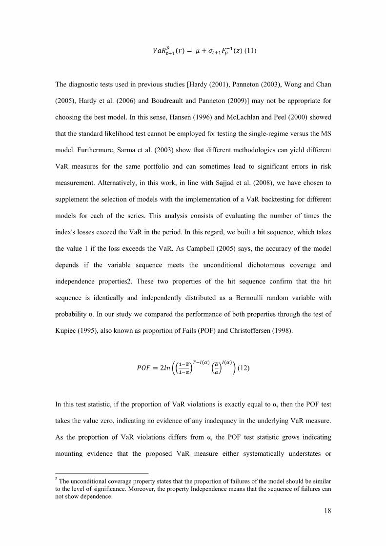
defl g (i) = + l mg () (11)

The diagnostic tests used in previous studies [Hardy (2001), Panneton (2003), Wong and Chan

(2005), Hardy et al. (2006) and Boudreault and Panneton (2009)] may not be appropriate for

choosing the best model. In this sense, Hansen (1996) and McLachlan and Peel (2000) showed

that the standard likelihood test cannot be employed for testing the single-regime versus the MS

model. Furthermore, Sarma et al. (2003) show that different methodologies can yield different

VaR measures for the same portfolio and can sometimes lead to significant errors in risk

measurement. Alternatively, in this work, in line with Sajjad et al. (2008), we have chosen to

supplement the selection of models with the implementation of a VaR backtesting for different

models for each of the series. This analysis consists of evaluating the number of times the

index's losses exceed the VaR in the period. In this regard, we built a hit sequence, which takes

the value 1 if the loss exceeds the VaR. As Campbell (2005) says, the accuracy of the model

depends if the variable sequence meets the unconditional dichotomous coverage and

independence properties2. These two properties of the hit sequence confirm that the hit

sequence is identically and independently distributed as a Bernoulli random variable with

probability α. In our study we compared the performance of both properties through the test of

Kupiec (1995), also known as proportion of Fails (POF) and Christoffersen (1998).

hnm = 2M oS pq pWEr(p) Spq

pWr(p)s (12)

In this test statistic, if the proportion of VaR violations is exactly equal to α, then the POF test

takes the value zero, indicating no evidence of any inadequacy in the underlying VaR measure.

As the proportion of VaR violations differs from α, the POF test statistic grows indicating

mounting evidence that the proposed VaR measure either systematically understates or

2 The unconditional coverage property states that the proportion of failures of the model should be similar

to the level of significance. Moreover, the property Independence means that the sequence of failures can

not show dependence.

19

overstates the portfolio's underlying level of risk. Christofersen's (1998) Markov test examines

whether or not the likelihood of a VaR violation depends on whether or not a VaR violation

occurred on the previous day.

hnm = #2M S ( t)uvvwuv-tuv-wu--( tv)uvvtvuv-( t-)u-vt-u--W (13)

Overall we can see that the models RSLN2 and RS-Garch pass all tests for all indices at

different levels of confidence, except in the case of the CAC-40 for a confidence level of 90%.

Something similar happens in the case of E-Garch model, with the exception of the series on the

IBEX-35, also exceeds the unconditional and Independence test. Similarly, the lognormal model

and the Garch, pass the test for low levels of confidence but, consistent with previous statistical

analysis, fail over for high levels of confidence in most of the indices. Finally, we would like to

point out that in some cases the best fitting model is specific to the data set used, hence the

selection process should be carried out ad hoc. Thus we can conclude that only RS-Garch

models pass the tests of normality, homoskedasticity, autocorrelation, unconditional coverage

and independence. Therefore, despite the greater complexity, are best suited to model the risk of

equity through internal models. Noted that RSLN2 model also presents a good balance between

simplicity and fit and only failed to pass the homoskedasticity test on the IBEX-35.

20

Table 7. POF and Christoffersen test for the four indices

Table 7 shows the p-values from the Likelihood Ratio test of Kupiec (1995) for unconditional coverage (Percentage of Failures) and

Christoffersen (1998) for independence, and the number of failures of each model.

VI. Comparison of Capital Requeriments Trough Markov Switching Models

Against Solvency II Starndard Model

In this section we compare the capital resulting from the use of previously tested

models, compared to the requirements established in the Standard Model. In this way we try to

show the differences in the quantification of risk capital for equity through regime switching

models that have shown a better fit to the time series of various European indices.

CAC-40

LOGNORMAL GARCH E-GARCH RSLN RSLN·3 RS-GARCH

POF TEST (99.5%) 0.0426 0.1635 0.4978 0.1224 0.0000 0.1226

POF TEST (99%) 0.0147 0.0147 0.3362 0.3093 0.0002 0.3093

POF TEST (95%) 0.1529 0.3747 0.5616 0.0598 0.1529 0.0533

POF TEST (90%) 0.8621 0.1960 0.8621 0.0065 0.0135 0.0001

CHRISTOFFERSEN LR TEST (99.5%) 0.7115 0.7820 0.8539 1.0000 0.3319 1.0000

FTSE-100

LOGNORMAL GARCH E-GARCH RSLN RSLN·3 RS-GARCH

POF TEST (99.5%) 0.1668 0.0095 0.0438 0.8505 0.8505 0.8505

POF TEST (99%) 0.0497 0.0497 0.1409 0.8505 0.7893 0.7893

POF TEST (95%) 0.0969 0.0299 0.0299 0.7893 0.3535 0.7640

POF TEST (90%) 1.0000 0.2959 0.2958 0.5424 0.5104 0.8307

CHRISTOFFERSEN LR TEST (99.5%) 0.0207 0.6446 0.7127 0.9271 0.9271 0.5791

IBEX-35

LOGNORMAL GARCH E-GARCH RSLN RSLN·3 RS-GARCH

POF TEST (99.5%) 0.1288 0.1288 0.1288 0.9377 0.1411 0.4278

POF TEST (99%) 0.5875 0.2606 0.5875 0.3753 0.0372 0.9118

POF TEST (95%) 0.2144 0.7126 0.5051 0.0439 0.0008 0.5633

POF TEST (90%) 0.8913 0.4507 0.4507 0.0671 0.0671 0.8913

CHRISTOFFERSEN LR TEST (99.5%) 0.7713 0.7713 0.7713 0.9232 1.0000 0.8467

DAX

LOGNORMAL GARCH E-GARCH RSLN RSLN·3 RS-GARCH

POF TEST (99.5%) 0.0077 0.0374 0.1488 0.8896 0.8896 0.1488

POF TEST (99%) 0.0404 0.0404 0.3043 0.3348 0.3348 0.6526

POF TEST (95%) 0.4543 0.4543 0.8907 0.1472 0.0701 0.4410

POF TEST (90%) 0.8419 0.6409 0.2639 0.0649 0.0093 0.6409

CHRISTOFFERSEN LR TEST (99.5%) 0.6366 0.7061 0.7061 0.9254 0.9254 0.7778

21

Capital requirements in the standard model (QIS4 and QIS5)

As discussed in the preceding paragraph, the quantification of risk in the Solvency II standard

model is made using the analytical VaR, which has been widely selected as a measure in the

financial markets, having analytical solution and allow the integration of different risks. The

parameters and assumptions used to calculate capital requirements correspond to the most

adverse shock that may occur to one year with a confidence level of 99.5%.

Thus, as we advance in the introduction to this paper, the amount of capital for equity risk in

QIS4 is calculated assuming a 32% drop for the investments in global developed market indices

(OECD / EEA countries ) and 45% for the rest of the market. These factors were determined

using average yields and net nominal exchange rate risk of the global index MSCI developed

markets for the period 1970/2005 (quarterly). After obtaining the individual quantities

associated with developed markets and other markets, these are added using a linear correlation

coefficient of 0.75. Since our work focuses on the analysis of a single index for a developed

market, the results should be compared with the factor of 32%. After the financial crisis, the

new quantitative impact study (QIS5) reduces this percentage to 30% but it introduces,

according to the new Solvency II Framework Directive (article 106), a symmetric adjustment of

-9 percent. The base levels of the two stresses are 39% and 49%, depending if the assets are

classified as global or other.

A new element that is included in QIS4 is the possibility of taking into consideration an

alternative, which considers a damping effect or "dampener". Under this new proposal would

also set the maximum load at 32 percent, but it is possible to obtain reductions in respect of that

amount depending on the duration of the liabilities and the cyclical component of the index. The

theoretical framework considers the existence of mean reversion in profitability of the indices

and therefore does not need to have as much equity when liabilities are not required in the short

term, since it is assumed that the market will recover. This buffering effect only applies to

liabilities with duration greater than three years. In this case the standard stressor (32%) is an

22

adjustment for damping cyclical component that takes into consideration the duration of

liabilities. The capital charge for risk of the overall index is then:

x>yzg|Q|,~ = dx ∙ 9 ∙ 9m(>) + (>) ∙ ()? + 0,32 ∙ (1 # )? (14)

Where:

- VM, market value of global index.

- α, Proportion of reserves linked to liabilities with duration greater tan 3 years.

- F(k) y G(k), Coefficients from next table, where k is liabilities duration.

K F(k) G(k)

3-5 años 29 % 0,20

5-10 años 26 % 0,11

10-15 años 23 % 0,08

+ 15 años 22 % 0,07

- C(t) is the cyclical component.

Capital requirements with regimen switching internal models

Here we present the results of estimating capital requirements to a portfolio that

contains any of the indices that have been used in this study. For this purpose a simulation of

100,000 scenarios for Latin Hypercube method to the time horizon of one year. Since the

adjustment has been made from monthly data and the calculation of capital annually, it is

necessary to perform temporary aggregation of simulated yields (Klein, 2002, Chan et al., 2008,

Chan et al., 2009). To analyze the problem of temporal aggregation is useful to define the

concept of A accumulation factor. Be P the monthly value unprocessed of time series (eg

series CAC40 index) at time t, for t = 0,1, ... n and define the performance logarithmic t-th

month as y = ln ,-. The series of logarithmic returns for the month m can be constructed as:

Y = ln (,-) = ∑ y;( )l (15)

For: T = 1, 2, ..., N, where N = [n/m] an integer.

23

The A factor accumulation or growth rate of the market value of the index can be defined as:

A = (,-) = exp(Y) (16) Therefore, the one year factor (m = 12) based on monthly logarithmic returns can be

obtained easily by:

A = exp(y + yl + yl + ⋯ + yl ) (17) And thus the value of the index in month 12, i.e. after one year is equal to:

P = PA .(18)

Table 8 shows the capital requirements that result from applying the different models previously

evaluated, calibrated as in the case of the standard model for VaR (99.5%). As can be seen these

factors significantly exceed the amount referred to in the standard model. In addition, the

normal return model, implicit in the calculation of the Solvency II capital, significantly

underestimates the amount of capital compared to other models. For all the indices evaluated,

the models of best fit, RSLN 2 and RS-GARCH regimes, capital charges result in substantially

higher than the standard model and those estimated by lognormal models, GARCH and E-

GARCH. This means that the use of simpler models could lead to an underestimation of the risk

actually assumed and the calculation of loads below those required. Furthermore, in the case of

IBEX, DAX, CAC, best-fit models suggest requirements around 39 percent, i.e. very close to

the stage of stress that has been recently included in QIS5. It is also important to note that the

FTSE generally presents a lower risk and, consequently, capital needs that in no case exceed 31

percent which shows that the determination of capital needs are specific to each risk factor.

24

Table 1. Comparison of capital requirements through alternative models

NORMAL GARCH EGARCH RSLN2 RSLN3 RSGARCH

CAC

VaR (99,5%) -32,4% -31,4% -34,5% -37,5% -38,5% -39,9%

VaR (99%) -29,6% -28,3% -29,9% -35,0% -36,5% -37,2%

DAX

VaR (99,5%) -32,5% -33,5% -35,3% -41,0% -40,2% -36,7%

VaR (99%) -29,8% -29,9% -31,4% -38,8% -36,5% -34,0%

IBEX

VaR (99,5%) -33,1% -35,1% -36,3% -40,4% -40,4% -36,6%

VaR (99%) -30,4% -31,2% -32,0% -38,2% -38,1% -33,9%

FTSE

VaR (99,5%) -25,2% -27,5% -27,7% -30,6% -31,0% -31,2%

VaR (99%) -23,0% -24,2% -24,1% -28,3% -28,7% -28,2%

VII. Conclusions

The new European Union solvency regulation for insurance companies, known as Solvency II,

involves the revision of standards for assessing the financial situation in order to improve the

measurement and control of risk. After the adoption in November 2009 of the new directive, is

being carried out the last quantitative impact study (QIS5) and the standard formula will be the

final. Under the new framework, the determination of capital requirements can be achieved

through a standard or internal models previously approved by the regulatory authority.

However, there have been few studies that attempt to analyze the models that can most

adequately measure the equity risk. The lognormal return model for analyzing the underlying

equity risk in the calculation of QIS5 has been chosen for simplicity and transparency and

provides a reasonable approximation for small time periods. However, the normality assumption

can seriously underestimate the tail of the loss distribution (extreme results) and inadequately

capture the variability in volatility. Other proposed alternatives in the literature like Garch

models are not able to capture sudden behavior changes in the market. The transformation of the

previous models introducing regime switching may be better suited to measuring the risk of

equity. For this reason the current study has examined the adequacy of Markov switching to

design internal models for the insurers' equity risk exposure. We have used monthly data from

25

four of the main european indices for the period between January of 1990 and January 2010.

The comparison of the models across different statistical criteria and backtesting show the

superiority of Markov switching over simpler models, for capturing insurers' equity risk. For all

the indices evaluated, regime switching models (RSLN 2 and RS-GARCH) show the best fit.

Furthermore, capital charges result in substantially higher than those estimated by lognormal

models, GARCH and E-GARCH. This means that the use of simple models could lead to an

underestimation of the actual risk assumed and the calculation of charges below those required.

Furthermore, in the case of IBEX, DAX, CAC, regime switching models suggest capital

requirements around 39 percent, i.e. very close to the stage that has been recently included in

QIS5. This means that the legislation revision in the last quantitative impact study is in line with

the capital charges estimated by the proposed models. The results are highly relevant as they

imply that European insurance companies that opt for internal models based on the assumption

of normality are underestimating the risk in accordance with developments in the European

equity markets. There is also evidence that the Garch models in their different forms, do not

capture enough adverse market movements and confirm the adequacy of RSLN2 and RS-Garch

to build internal models focused in the assessment and measurement of equity risk.

26

Bibliography

Ahlgrim, K. C.; D'Arcy, S. P. and Gorvett, R. W. (2004a) Asset/liability modeling for insurers

Incorporating a regime/switching process for equity returns, in Dynamic Financial Analysis model

ASTIN Colloquium 2004.

Ahlgrim, K. C.; D'Arcy, S. P. y Gorvett, R. W. (2004b) Modeling of Economic Series Coordinated with

Interest Rate Scenarios, Available in http//casact.org/research/econ/.

Akaike, H. (1973) Information Theory and an Extension of the Maximum Likelihood Principle, in The

Second International Symposiumon Information Theory, pp. 267–281. Hungary Akademiai Kiado.

Ball, C. A. and Torous, W. N., (1983) A simplified jump process for common stock returns, Journal of

Financial and Quantitative Analysis ,18, No. 1, pp. 53-65.

Bayliffe D. and Pauling, B. (2003) Long Term Equity Returns, In Stochastic Modeling Symposium, 4/5

September Toronto.

Boudreault and Panneton (2009) Multivariate Models of Equity Returns for Investment Guarantees

Valuation, *orth American Actuarial Journal, 13, No.1, pp. 36-53.

Cai, J. (1994) A Markov model of unconditional variance in ARCH, Journal of Business and Economic

Statistics, 12, 309-316.

Campbell, C. (2005) A Review of Backtesting and Backtesting Procedures, Finance and Economics

Discussion Series, Divisions of Research & Statistics and Monetary Affairs, Federal Reserve Board,

Washington, D.C.

CEIOPS (2007) Calibration of the underwriting risk, market risk and MCR. CEIOPS/ FS/14/07.

CEIOPS (2008) QIS4 Technical Specifications. MARKT/2505/08.

Commission of the European Communities (2009) Solvency II Directive.

Christoffersen P. (1998) Evaluating Interval Forecasts, International Economic Review, 39, 841-862.

D’Arcy, S.P.; Gorvett, R. W.; Herbers, J. A.; Hettinger, T. E.; Lehmann, S. G. and Miller, M. J. (1997)

Building a Public Access PC/Based DFA Model, in CAS Forum, pp. 1-40.

D’Arcy, S. P.; Gorvett, R.W.; Hettinger, T.E. and Walling, III R.J. (1998) Using the Public Access

Dynamic Financial Analysis Model. A Case Study, in CAS Forum, pp. 53-118.

D’Arcy, S.P. and Gorvett, R. (2004) The Use of Dynamic Financial Analysis to Determine Whether an

Optimal Growth Rate Exists for a Property/Liability Insurer, Journal of Risk and Insurance, 71, No. 4,

pp. 583-615.

27

Engle, R. F. (1982) Autoregressive conditional heteroskedasticity with estimates of the variance of UK

inflation, Econometrica, 50, No.4, pp. 987-1008.

Engle, R.F. and Bollerslev, T. (1986) Modelling the persistence of conditional variance, Econometric

Reviews, 5, No. 1, pp. 1-50.

Fama, E. F. (1963) Mandelbrot and the Stable Paretian Hipothesis Journal of Business, 36, No. 4, pp.

420-429.

Fama, E. F. (1965) The Behaviour of Stock Market Prices, Journal of Business, 38, No. 1, pp. 34-105.

Glosten, L,. Jagannthan, R. and Runkle, D. (1993) On the Relation between the Expected Value and the

atility of the Nominal Excess Return on Stocks, Journal of Finance, 48, No. 5, pp. 1779-1801.

Gray, S.F., (1996) Modeling the conditional distribution of interest rates as a regime switching process.

Journal of Financial Economics, 42, 27-62.

Gray, J. B. and French, D. W. (1990) Empirical Comparisons of Distributional Models for Stock Index

Returns. Journal of Business Finance and Accounting, 17, No. 3, pp. 451-459.

Hamilton, J. D. (1989) A New Approach to the Economic Analysis of Non stationary Time Series.

Econometrica, 57, No 2, pp. 357-84.

Hamilton, J. D (1994) Time Series Analysis. Princeton University Press.

Hamilton, J.D. and Susmel, R. (1994) Autoregressive conditional heteroscedasticity and changes in

regime, Journal of Econometrics, 64, 307-333.

Hamilton (2005) Regime-Switching Models, Palgrave Dictionary of Economics.

Hansen, B. E., (1996) Erratum the Likelihood Ratio test under nonstandard conditions Testing the

Markov switching model of GNP, Journal of Applied Econometrics, 11, 195-198.

Hardy, M.R. (1999) Stock return models for segregated fund guarantees, Segregated Funds Symposium

Proceedings, Canadian Institute of Actuaries.

Hardy, M. R. (2001) A Regime Switching Model of Long/Term Stock Returns, *orth American Actuarial

Journal, 5, No. 2, pp. 41-53.

Hardy, M. R. (2003) Investment Guarantees; Modeling and Risk Management for Equity Linked Life

Insurance. Wiley, New York.

Hardy, M. R.; Freeland, R. K. and Till, M. C. (2006) Validation of Long/Term Equity Return Models for

Equity/Linked Guarantees, *orth American Actuarial Journal, 10, pp. 28-47.

28

Henry, O. (2009) Regime switching in the relationship between equity returns and short-term interest

rates in the UK, Journal of Banking & Finance 33 (2009) 405-414.

Hibbert, J.; Mowbray, P. and Turnbull, C. (2001) A Stochastic Asset Model & Calibration for Long/Term

Financial Planning Purposes, Technical Report, Barrie & Hibbert Limited.

Jarque, C. M. and Bera, A.K (1980) Efficient Tests for Normality, Homoscedasticity and Serial

Independence of Regression Residuals, Economics Letters, 6, pp. 255-259.

Jarque, C. M. and Bera, A.K (1987) A Test for Normality of Observations and Regression Residuals,

International Statistical Review, 55, No. 2, pp. 163-72.

Klaassen, F. (2002) Improving GARCH utility forecasts with regime switching Garch, Empirical

Economics, 27, 363-394.

Kupiec P. (1995) Techniques for Verifying the Accuracy of Risk Management Models, Journal of

Derivatives, 3, 1995, 73-84.

Lintner, J. (1965) The Valuation of Risk Assets and the Selection of Risky Investments in Stock

Portfolios and Capital Budgets, Review of Economics and Statistics , 47, No. 1, pp. 13-37.

Mandelbrot, B. (1963 The Variation of Certain Speculative Prices, Journal of Business, 36, No. 4, pp.

394-419.

Ljung, G. y Box, G. (1979) On a Measure of Lack of Fit in Time Series Models, Biometrika, 66, pp. 265-

270.

Marcucci, J. (2005) Forecasting stock market atility with Regime-Switching GARCH models, Studies in

*onlinear Dynamics & Econometrics, 9, 4, Article 6.

McLachlan, G. J. and Peel, D. (2000) Finite Mixture Models, New York John Wiley& Sons.

Mossin, J. (1966) Equilibrium in a Capital Asset Market, Econometrica, 34, No. 4, pp. 768-783.

Nelson, D.B. (1991) Conditional heteroscedasticity in asset returns a new approach, Econometrica, 59,

pp. 347-370.

Panneton, C.M. (2003) Mean/Reversion in Equity Models in the Context of Actuarial Provisions for

Segregated Fund Investment Guarantees, 2003 Stochastic Modeling Symposium Proceedings, Canadian

Institute of Actuaries.

Panneton, C.M. (2005) Practical Implications of Equity Models in the Context of Actuarial Provisions for

Segregated Funds Investment Guarantees, Master Thesis, Université Laval.

29

Panneton, C. M. (2006) A Review of the CIA Calibration Criteria for Stochastic Modeling, CIA

Stochastic Modeling Symposium, Canadian Institute of Actuaries.

Praetz, P. D. (1972) The Distribution of Share Price Changes, Journal of Business, 45, No. 1, pp. 49-55.

Sarma, M., Thomas, S. and Shah, A. (2003) Selection of Value-at-Risk models, Journal of Forecasting,

22, 337-358.

Sajjad,R.; Coakley,J. and Nankervis,J. (2008)Markov-Switching GARCH Modelling of Value at Risk,

Studies in Nonlinear Dynamics &Econometrics, ume 12, Issue 3, pp.1-29.

Schwarz, G. (1978) Estimating the dimension of a Model. The Annals of Statistics, 6, pp. 461/464.

Sharpe, W. (1964) Capital Asset Prices A Theory of Market Equilibrium Under Conditions of Risk,

Journal of Finance, 19, No. 3, pp. 425-442.

Silverman, B. W. (1986) Density Estimation. London Chapman and Hall.

Schmeiser, H., (2004) New Risk/Based Capital Standards in the EU. A Proposal Based on Empirical

Data, Risk Management and Insurance Review, 7, No. 1, pp. 41-52.

Taylor, S.J. (1986) Modeling Financial Time Series, Wiley, New York.

Wong, C. S. and Chan, W. S. (2005) Mixture Gaussian Time Series Modeling of Long/Term Market

Returns, *orth American Actuarial Journal, 9, No. 4, pp. 83-94.

Wong, C. S. and Li, W. K. (2000) On a Mixture Autoregressive Model Journal of the Royal Statistical

Society B62, pp. 95-115.

Wong, C. S. and Li, W. K. (2001) On a Mixture Autoregressive Conditional Heteroscedastic Model,

Journal of the American Statistical Association, 96, pp. 982-995.