Estimating Exposure via Mathematical Modeling for On-Site

Worker Health Risk Assessment

Mark Nicas, PhD, MPH, CIH School of Public Health

University of California, Berkeley

Our Goal

Estimate the concentration of a toxic chemical in an individual’s breathing zone during future chemical use scenarios. There are two approaches.

The Field Measurement Approach

Directly measure the breathing zone concen-trations during many different use scenarios so we have measurements for all future scenarios. Need to make repeat measurements per scenario. But … there are many unique scenarios and it is costly to make measurements, so this approach is not feasible, in general.

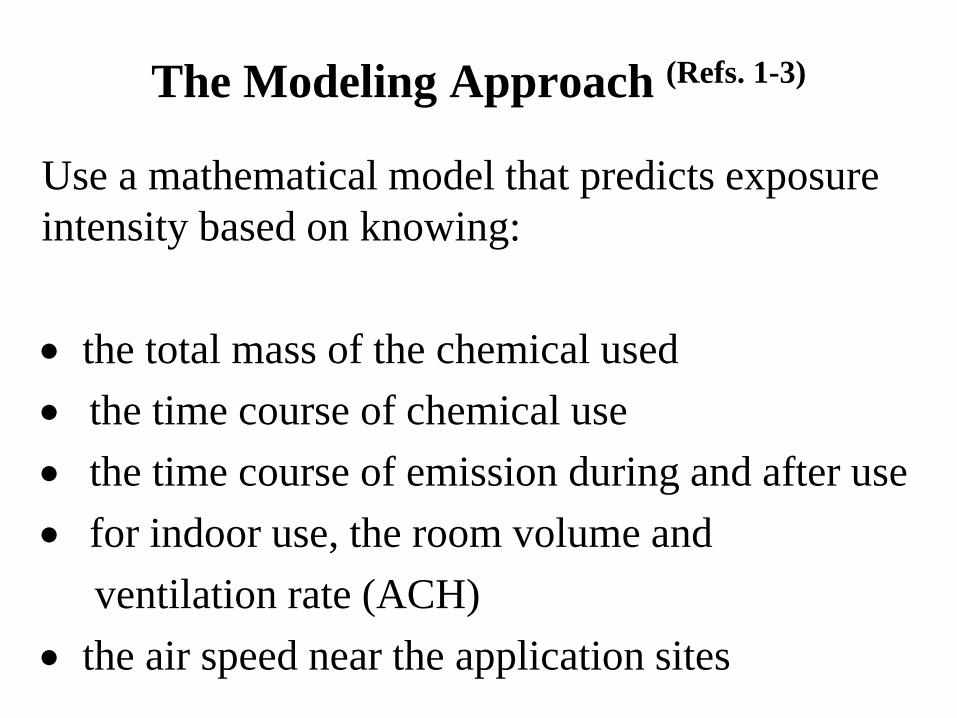
The Modeling Approach (Refs. 1-3)

Use a mathematical model that predicts exposure intensity based on knowing: • the total mass of the chemical used • the time course of chemical use • the time course of emission during and after use • for indoor use, the room volume and ventilation rate (ACH) • the air speed near the application sites

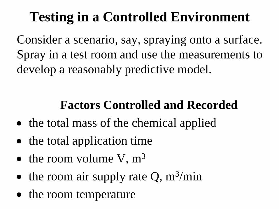
Testing in a Controlled Environment Consider a scenario, say, spraying onto a surface. Spray in a test room and use the measurements to develop a reasonably predictive model. Factors Controlled and Recorded • the total mass of the chemical applied • the total application time • the room volume V, m3 • the room air supply rate Q, m3/min • the room temperature

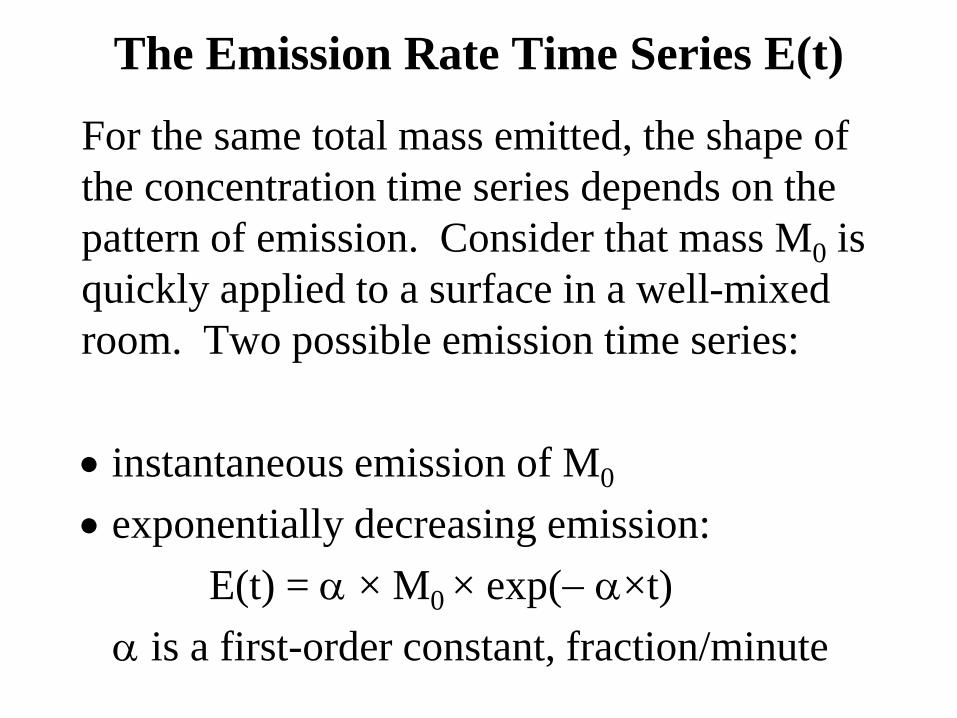
The Emission Rate Time Series E(t)

For the same total mass emitted, the shape of the concentration time series depends on the pattern of emission. Consider that mass M0 is quickly applied to a surface in a well-mixed room. Two possible emission time series: • instantaneous emission of M0 • exponentially decreasing emission: E(t) = α × M0 × exp(− α×t) α is a first-order constant, fraction/minute

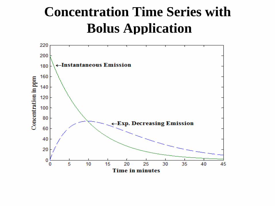
Concentration Time Series with Bolus Application

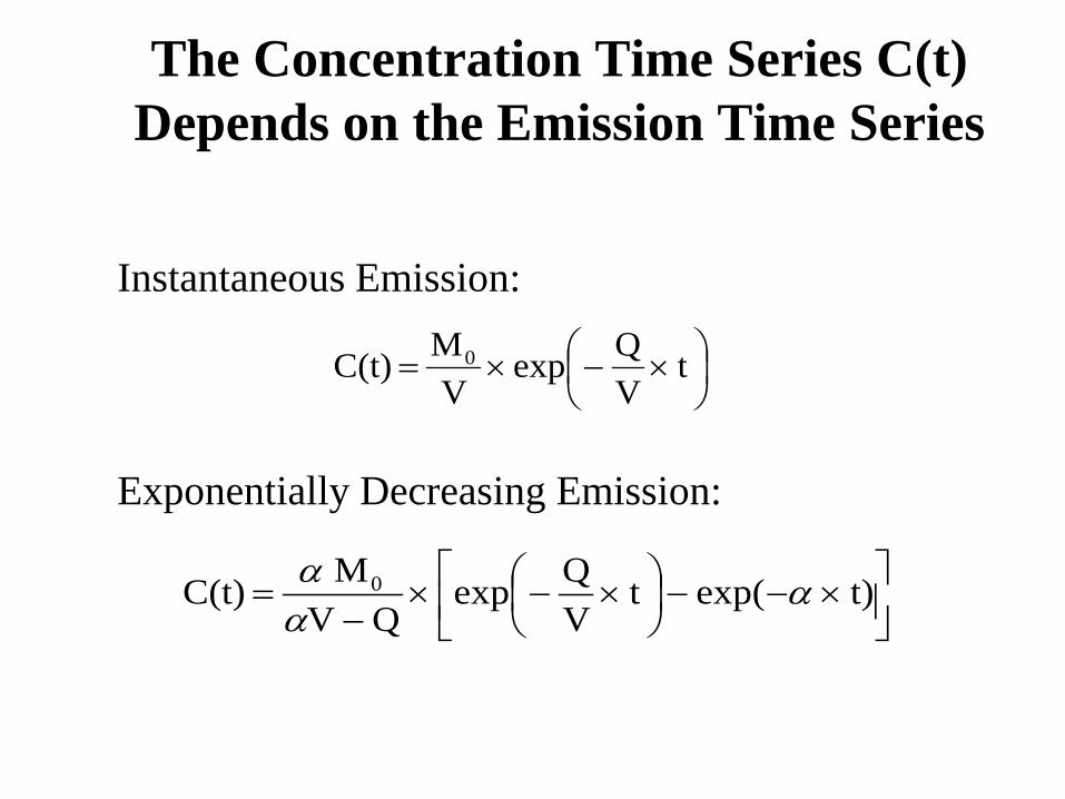
The Concentration Time Series C(t) Depends on the Emission Time Series

Instantaneous Emission: Exponentially Decreasing Emission:

×−−

×−×

−= t)exp( t

VQexp

Q V M C(t) 0 α

αα

×−×= t

VQexp

VM C(t) 0

Some Items to Note

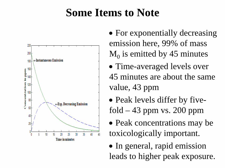
• For exponentially decreasing emission here, 99% of mass M0 is emitted by 45 minutes • Time-averaged levels over 45 minutes are about the same value, 43 ppm • Peak levels differ by five-fold – 43 ppm vs. 200 ppm • Peak concentrations may be toxicologically important. • In general, rapid emission leads to higher peak exposure.

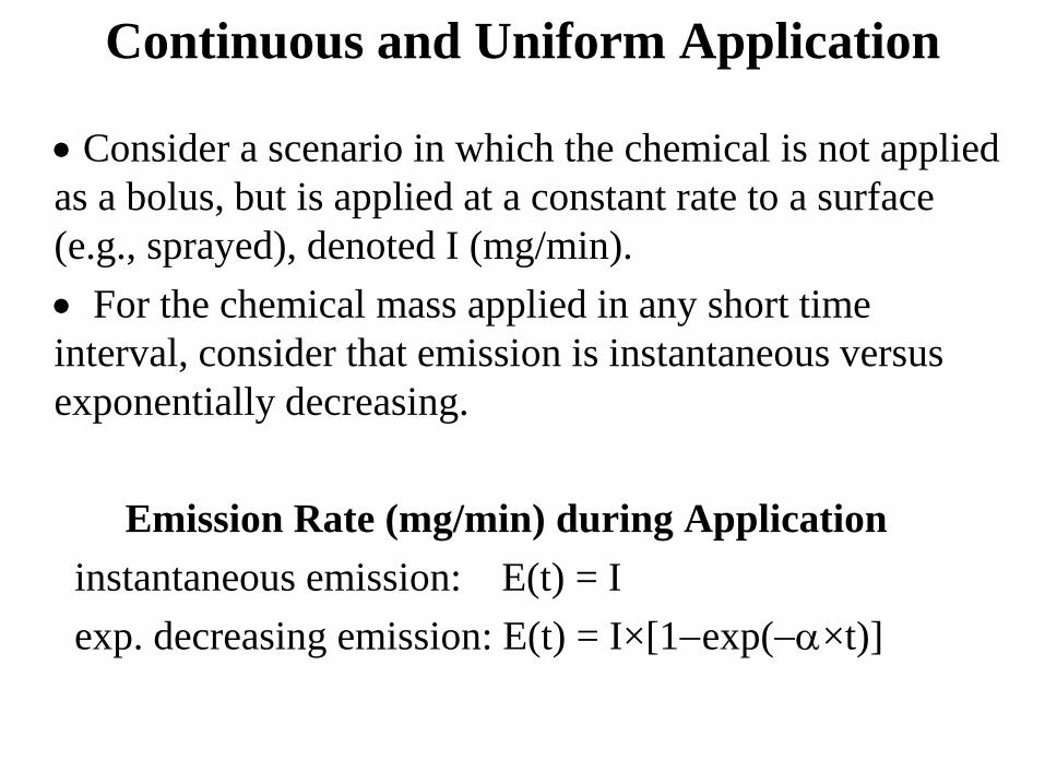
Continuous and Uniform Application

• Consider a scenario in which the chemical is not applied as a bolus, but is applied at a constant rate to a surface (e.g., sprayed), denoted I (mg/min). • For the chemical mass applied in any short time interval, consider that emission is instantaneous versus exponentially decreasing. Emission Rate (mg/min) during Application instantaneous emission: E(t) = I exp. decreasing emission: E(t) = I×[1−exp(−α×t)]

Concentration Time Series with Continuous Uniform Application

The Concentration Time Series C(t) Depends on the Emission Time Series

Instantaneous Emission: Exponentially Decreasing Emission:

×−−×= t

VQexp 1

QI C(t)

( )

×−−

×−×

−+

×−−×= texp t

VQexp

VQI t

VQexp 1

QI C(t) α

α

Some Items to Note

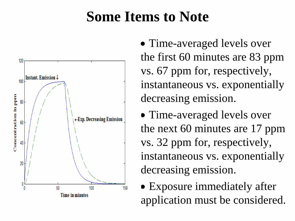
• Time-averaged levels over the first 60 minutes are 83 ppm vs. 67 ppm for, respectively, instantaneous vs. exponentially decreasing emission. • Time-averaged levels over the next 60 minutes are 17 ppm vs. 32 ppm for, respectively, instantaneous vs. exponentially decreasing emission. • Exposure immediately after application must be considered.

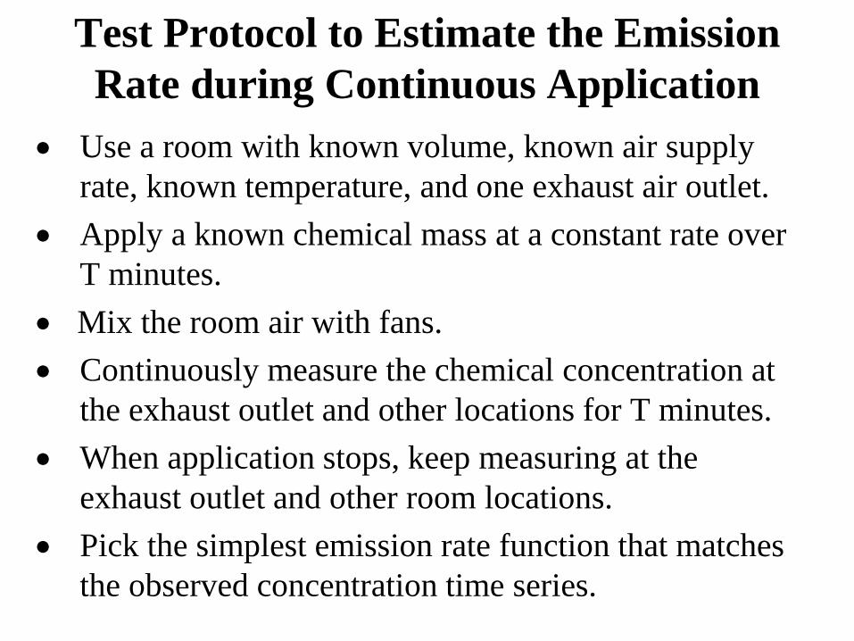
Test Protocol to Estimate the Emission Rate during Continuous Application

• Use a room with known volume, known air supply rate, known temperature, and one exhaust air outlet.

• Apply a known chemical mass at a constant rate over T minutes.

• Mix the room air with fans. • Continuously measure the chemical concentration at

the exhaust outlet and other locations for T minutes. • When application stops, keep measuring at the

exhaust outlet and other room locations. • Pick the simplest emission rate function that matches

the observed concentration time series.

Like in Real Estate, Location is Key

• In addition to the chemical emission rate, consider the location of the individual relative to the source of emission. • In general, the closer one is to the source of emission, the higher one’s exposure intensity. • Location affects how we choose to describe chemical dispersion in air.

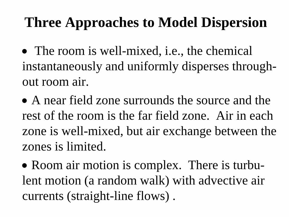
Three Approaches to Model Dispersion

• The room is well-mixed, i.e., the chemical instantaneously and uniformly disperses through-out room air. • A near field zone surrounds the source and the rest of the room is the far field zone. Air in each zone is well-mixed, but air exchange between the zones is limited. • Room air motion is complex. There is turbu-lent motion (a random walk) with advective air currents (straight-line flows) .

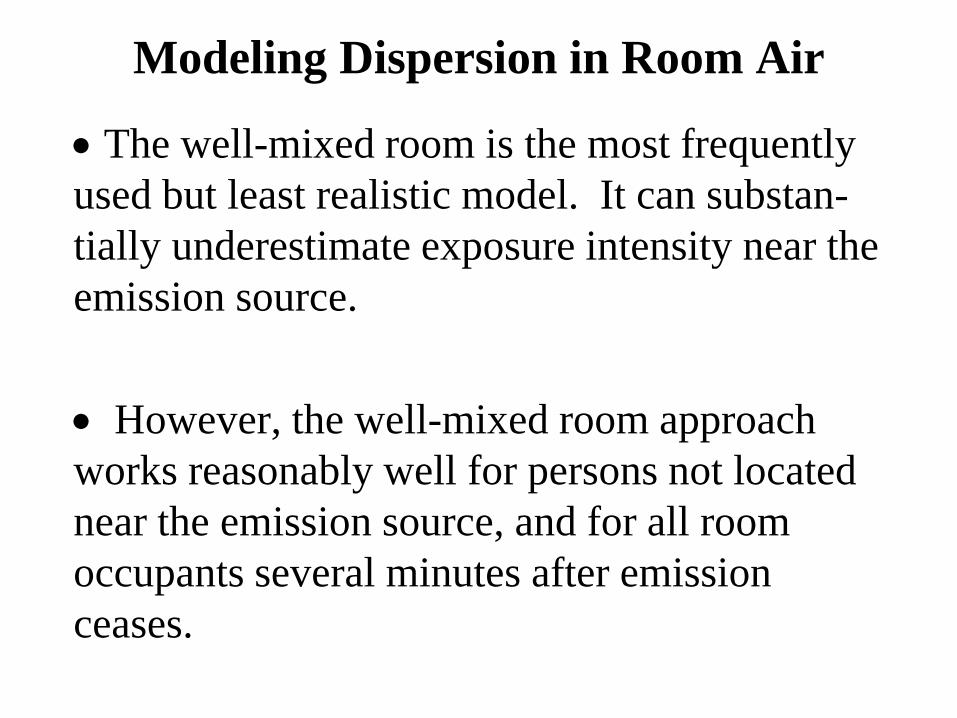
Modeling Dispersion in Room Air

• The well-mixed room is the most frequently used but least realistic model. It can substan-tially underestimate exposure intensity near the emission source. • However, the well-mixed room approach works reasonably well for persons not located near the emission source, and for all room occupants several minutes after emission ceases.

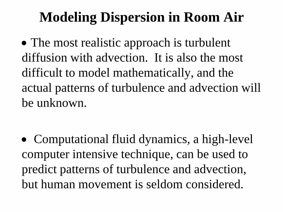
Modeling Dispersion in Room Air

• The most realistic approach is turbulent diffusion with advection. It is also the most difficult to model mathematically, and the actual patterns of turbulence and advection will be unknown.

• Computational fluid dynamics, a high-level computer intensive technique, can be used to predict patterns of turbulence and advection, but human movement is seldom considered.

Modeling Dispersion in Room Air

• The near field/far field (NF/FF) dispersion approach can be used when the individual is close to the emission source. • It is a compromise between the over-simplicity of the well-mixed room model and the complexity of modeling turbulent diffusion with advection.

The NF/FF Model

• One poses a geometry for the NF zone that contains the individual’s breathing zone. For example, if chemical is being used on a small work table, the NF zone might be a box of air with its base on the table and its height from the base to the individual’s face. • The NF zone has volume (VNF) and a free surface area (FSA) through which air moves. No air leaves the NF zone directly to outside the room.

The NF/FF Model • Assume there is a random air speed S (it could also be measured) at the interface of the NF and FF zones. Default values are S = 10 fpm when there are no strong sources of air currents near the NF zone, and S = 50 fpm when there are. • Airflow rate into and out of the NF zone: β (m3/min) = ½ × S × FSA • The room has volume V and air supply rate Q.

The NF/FF Model

If chemical emission is constant at rate I (mg/min), there are exact, gnarly equations for the concentrations in the NF and FF zones. Here are approximations. Far Field: Near Field:

×−−×+

×−−×≅ t

Vexp 1 I t

VQexp 1

QI (t)C

NFNF

ββ

×−−×≅ t

VQexp 1

QI (t)CFF

The NF/FF Model - Constant Application and Instantaneous Emission

0 10 20 30 40 50 600

10

20

30

40

50

60

70

80

90

100

Time in minutes

Con

cent

ratio

n in

ppm

CFF(t) ↓

CNF(t) ↓

Some Items to Note

• Time-averaged levels over the first 60 minutes are 68 ppm vs. 26 ppm for, respectively, the NF zone vs. the FF zone. • At steady state, CFF = I/Q and CNF = I/Q + I/ β. • In general, the larger the room, the higher the Q value with little effect on the β value. In turn, the relative difference between the NF and FF con-centrations increases.

0 10 20 30 40 50 600

10

20

30

40

50

60

70

80

90

100

Time in minutes

C

on

cen

tra

tio

n i

n p

pm

CFF(t) ↓

CNF(t) ↓

Test Protocol for the NF/FF Model • Use a room with known volume V, known air supply rate Q, known temperature, and one exhaust air outlet. • Apply a known chemical mass at a constant rate over T minutes. • Do not mix the room air with fans. Measure the air speed S near the application point. • Continuously measure the chemical concentration in the BZ, at the exhaust outlet and at other locations. • Assess if the chosen emission rate and the NF/FF dispersion pattern lead to predictions that reasonably match the observed BZ concentrations.

Some Past Test Data for the NF/FF Model

Process Measured Predicted methanol to NF: 57 ppm 65 ppm clean wafers FF: 16 ppm 25 ppm (Ref. 4) NF: 115 ppm 135 ppm FF: 51 ppm 100 ppm cyclohexane NF: 68 ppm 71 ppm on metal parts FF: 44 ppm 35 ppm (Ref. 5) NF: 51 ppm 37 ppm FF: 52 ppm 35 ppm

Outdoor Air Scenarios

• Pose a geometry for the NF zone such that it contains the emission source and the individual’s breathing zone. • Wind speeds can be quite variable across time. I suggest that if the chemical application is at ground level, assume S = 2 mph, and if it’s higher up, assume 5 or 10 mph. • Treat the NF zone as a “well-mixed room” with volume VNF and ventilation rate β. Because chemical leaving the NF zone is greatly diluted, ignore the FF zone effect.

Outdoor Air Scenarios

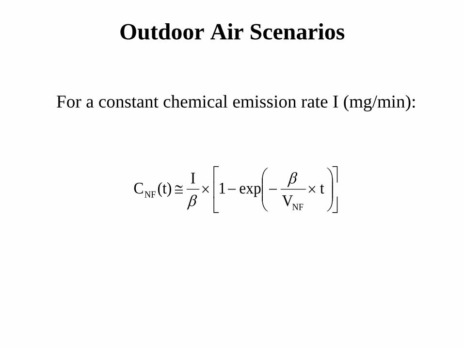
For a constant chemical emission rate I (mg/min):

×−−×≅ t

Vexp 1 I (t)C

NFNF

ββ

Utility of Mathematical Modeling

• In general, one can combine any chemical emission rate function with any dispersion pattern in air. • Once the model is formulated, the inputs can be made specific for the scenario of concern to predict the breathing zone concentrations. • There is always uncertainty in a model estimate, but there is also substantial variability in exposure measurements when performing nominally the same task. • If one wants to confirm model predictions for a specific scenario, direct exposure measurements can be made in the field when that specific chemical use task is performed.

References 1. Mathematical Models for Estimating Occupational Exposure to Chemicals, 2nd Edition, editors CB Keil, CE Simmons and TR Anthony, American Industrial Hygiene Association, Fairfax, VA, 2009 2. Nicas M: “Mathematical Modeling of Indoor Air Contaminant Concentrations,” Chapter 17 (pages 661-693), Volume 2, Evaluation and Control, Pattys Industrial Hygiene Sixth Edition, Eds. B Cohrssen and V Rose, John Wiley & Sons, Inc., New York, NY, 2010 3. Nicas M: “Quantitative Surveying – Application of Mathematical Modeling to Estimate Air Contaminant Exposure,” in Modern Industrial Hygiene, Volume I, Recognition and Evaluation of Chemical Agents, Second Edition, by Jimmy L. Perkins, ACGIH, Cincinnati, OH, 2008 4. Gaffney S, et al.: Worker exposure to methanol vapors during cleaning of semiconductor wafers in a manufacturing setting, J. Occup. Environ. Hygiene 5:313-324, 2008 5. Spencer J and M Plisko: A comparison study using a mathematical model and actual exposure monitoring for estimating solvent exposure during disassembly of parts, J. Occup. Environ. Hygiene 4:253-259, 2007

References 6. Nicas M: Using mathematical models to estimate exposure to workplace air contaminants, Chem. Health Safety 10:14-21, 2003 7. Jayjock M., et al.: The Daubert standard as applied to exposure assessment modeling using the two-zone (NF/F) model estimation of indoor air breathing zone as an example, J. Occup. Environ. Hygiene 8:D114-122, 2011.