FACULTEIT ECONOMIE EN BEDRIJFSKUNDE

TWEEKERKENSTRAAT 2 B-9000 GENT

Tel. : 32 - (0)9 – 264.34.61 Fax. : 32 - (0)9 – 264.35.92

WORKING PAPER

Estimating Europe’s Natural Rates from a forward-looking Phillips curve

Tino Berger

January 2008

2008/498

D/2008/7012/07

Estimating Europe’s Natural Rates from a forward-looking

Phillips curve ∗

Tino Berger†

January 9, 2008

Abstract

This paper re-estimates potential output, the NAIRU, and the core inflation rate using

aggregated euro area data. The empirical model consists of a Phillips curve linking inflation

to unemployment. An Okun-type relationship is used to link the output gap to cyclical unem-

ployment. Using recent developments in the field of New Keyenesian economics, the Phillips

curve is forward-looking. The model further accounts for new developments in unobserved

component models by allowing (i) for correlation between shocks to the trend and the cycle

and (ii) structural breaks in the drift of potential output.

1 Introduction

Measuring equilibrium rates of key macroeconomic variables and the resulting gaps has a long-

standing history in the economic literature. Since the seminal contribution of Burns and Mitchell

(1946) several studies estimated business cycles using various different concepts of equilibrium

rates and different statistical techniques to extract them from the data. The deviation of actual

output from its long-run level, referred to as potential output, provides an estimate about the

cyclical position of the economy. A positive output gap, i.e. actual output exceeds potential

output, implies inflationary pressure as demand exceeds supply. A closely related concept is that

of a natural rate of unemployment and has been pioneered by Friedman (1968) and Phelps (1968)

who claim that unemployment is at its natural level when neither inflationary nor deflationary∗I would like to thank Gert Peersman and Gerdie Everaert for useful comments and suggestions. I also acknowl-

edge financial support from the Interuniversity Attraction Poles Program - Belgian Science Policy, contract no.P5/21. The usual disclaimer applies

†SHERPPA, Ghent University, Tino.Berger@UGent.be, www.sherppa.be

1

pressure emanates from the labour market. This is called the non-accelerating-inflation-rate of

unemployment (NAIRU).

A popular method to estimate natural rates is the Unobserved Component (UC) model in which

trend and cycle are treated as latent state variables, the former modelled as a non-stationary

process while the cycle is mean reverting. After casting the model in state-space form, it can

be estimated using the Kalman filter. The UC model, pioneered by Harvey (1985), Watson

(1986), and Clark (1987), typically assumes zero correlation between shocks to the trend and the

cycle. However, Morley et al. (2003) showed that this restriction strongly influences the resulting

decomposition. They further showed that, under certain conditions, this correlation is identified

and can be estimated. Moreover, when focusing on output decomposition, Perron and Wada

(2005) showed the importance of properly specifying a process for potential output that is capable

to account for structural breaks. Specifically they argue that modelling trend growth as either

deterministic or a simple random walk yields to an estimate in which the trend is very close to

actual output, leaving little to the cycle. Hence, it does not accord with what is commonly viewed

as a business cycle.

The existing literature is dominated by studies that focus on the US economy. Recent con-

tribution include Basistha and Nelson (2007) who estimate the US output gap from a bivariate

system combining inflation and output through a forward-looking Phillips curve. Additionally

they allow for correlated trend and cycle shocks. Domenech and Gomez (2006) estimate potential

output, core inflation, and the NAIRU from a model that combines information contained in real

GDP, inflation, unemployment, and investment. Their model includes a forward-looking Phillips

curve and allows for some volatility breaks. The literature that focuses on the euro area is much

scarcer. As an exception Ruenstler (2002) estimates the real-time output gap for the euro area

and studies its reliability over different model specification. Fabiani and Mestre (2004) focus on

estimating the euro area NAIRU using a backward-looking Phillips curve and do not allow for

correlated trend cycle shocks.

This paper re-estimates potential output, the NAIRU, and the core inflation rate using aggre-

gate euro area data. The empirical model, building on Apel and Jansson (1999a,b), consists of a

Phillips curve linking inflation to unemployment. An Okun-type relationship is used to link the

output gap to cyclical unemployment. Using recent developments in the field of New Keyenesian

economics, the Phillips curve is forward-looking. This allows for a more model based interpretation

of the estimated gaps. The model further accounts for the new developments in UC models by

allowing (i) for correlation between shocks to the trend and the cycle and (ii) structural breaks in

the drift of potential output. In order to investigate the importance of these points two alternative

models are estimated and compared to the baseline specification.

The rest of the paper is organised as follows. Section 2 briefly reviews recent developments in

trend-cycle decomposition with regard to UC models. Section 3 outlines and estimates the model.

In section 4 the results are presented. Section 5 concludes.

2 Recent developments in trend-cycle decomposition

Natural rates such as potential output or the NAIRU are not directly observable and therefore

have to be estimated using statistical methods. Various methodologies have been suggested for

estimating natural rates and the corresponding gaps. They can be divided into two groups, purely

statistical and economic based. The latter approach estimates a production function and obtains

a measure of potential output from various factor inputs multiplied by total factor productivity.

Recent contribution include Proietti et al. (2007) and Roeger (2006). However the focus here is

on the statistical methods to estimate natural rates.1

Among the widely used methods are the filter of Hodrick and Prescott (1997) (HP), the Band-

Pass (BP) filter of Baxter and King (1999), the Beveridge and Nelson (1981) decomposition, and

the UC model. The HP and the BP filter obtain trend estimates by imposing smoothness a priori.

In contrast the BN decomposition and UC models have the advantage of not imposing smoothness

but ’let the data speak’ as much as possible. The BN decomposition is based on an unconstrained

ARIMA model where the trend is defined as the long-run forecast and the cycle as the difference

between the trend component and the actual data. As a consequence, the same innovation drives

trend and cyclical component implying that they are perfectly negatively correlated. Similar to the

BN decomposition the UC trend-cycle model also requires identification of the trend, i.e. a law of

motion has to be specified. However, the UC model in state space form is not based on modelling

first differences but models the series as the sum of the trend and the cyclical component. Thus,1See Canova (1998) for an overview and a discussion of the differences between statistical and economic ap-

proaches.

one must also specify a law of motion for the cycle. The two components are driven by different

innovations which are typically assumed to be uncorrelated. Although the BN decomposition

and the UC model are purely statistical approaches without imposing smoothness of the trend

a priori they lead to very different trend cycle decomposition. The BN decomposition leads to

a trend estimate which closely follows the observed data. Thus the resulting cycle is very small

and noisy and can hardly be seen as a business cycle. To the contrary, the cycle obtained from a

UC model is large and persistent and accords well with business cycle chronologies, such as the

NBER for the US or the CEPR for the euro area. The conflicting results suggest that either the

BN decomposition or the UC model is not supported by the data.

In a recent paper Morley et al. (2003) show that this puzzling feature is caused by the assump-

tion of zero correlation between shocks to trend and cycle. They further show that the correlation

is identified and can be estimated if the specified cycle bears rich enough dynamics. In a univariate

trend-cycle decompositions where the trend is a random walk the cycle needs to be specified as an

ARMA(p, q) process with p ≥ q + 2. When applying this correlated UC model to US GDP they

found that the estimated correlation between shocks to the trend and cycle is very high and the

estimated trend is virtually identical to the BN decomposition. Thus, although the assumption

of zero correlation leads to reasonable business cycles, it clearly is at odds with the data. The

results of Morley et al. lead to a new strand of literature which is labelled correlated unobserved

components models. Contribution in this line of research include, among others, Basistha (2007),

Basistha and Nelson (2007), and Sinclair (2007).

The importance of relaxing the zero correlation assumption in UC models solved one puzzle

but raised another. How should one interpret the resulting components? The estimated cyclical

components in Morley et al. (2003) is, by construction transitory, but noisy and small in magnitude.

On the other hand the trend component follows the data closely, implying a dominant role for

permanent shocks in explaining real GDP in US postwar data. At first sight this result confirms

neoclassical business cycle theory which ascribes changes in real GDP to movements in production

due to technology shocks. By analysing this issue in detail Perron and Wada (2005) argued

that the small cycle is the result of a misspecified model. Specifically they showed that if one

accounts for a single break in the slope of the trend function the delivered cycle from both, the

BN decomposition and the correlated UC model, is large and persistent and accords with the

NBER chronology. Typically the drift of the trend is either treated as deterministic or modelled

as a random walk (see e.g. Stock and Watson, 1998). It is important to note that even the latter

approach can not adequately account for infrequent shifts in the drift of the trend function. As

Perron and Wada point out the variance of an estimated random walk drift is very small implying

a drift that changes only little but every period though. As a consequence, if there are infrequent

but large shifts in the slope of the trend function, the random walk drift is inadequate to capture

them.

The result of a small and noisy cycle seems to be more important in univariate models. Studies

that estimate multivariate models typically find the cycle to be large and persistent. Intuitively

this might be due to the additional information contained in e.g. the inflation rate. Neverthe-

less, potential output remains misspecified if there are infrequent but large shifts which are not

accounted for.

3 A multivariate correlated unobserved component model

This section lays out a multivariate correlated UC model that consists of output, unemployment,

and inflation. Euro area data, which are aggregate series for 12 countries2, are taken from the area-

wide model of Fagan et al. (2005) and range from 1970 until 2005. The unemployment rate, ut, is

the quarterly unemployment rate. For inflation, πt, the first difference of the log of the seasonally

adjusted quarterly GDP deflator is used. Output is the log of seasonally adjusted quarterly GDP

in constant prices.

3.1 Unemployment Decomposition

The rate of unemployment is disentangled into two components, a non-stationary trend component

u∗t , and a cyclical component uct

ut = u∗t + uct . (1)

2Austria, Belgium, Finland, France, Germany, Greece, Ireland, Italy, Luxembourg, Netherlands, Portugal, andSpain.

The latter is modelled as a AR(2) process

uct = φ1u

ct−1 + φ2u

ct−2 + ηc

t , (2)

where ηct is a Gaussian mean zero white noise error term. The AR(2) specification allows cycli-

cal unemployment to exhibit the standard hump-shaped pattern. The NAIRU, i.e. the trend

component in the unemployment rate, is specified as a random walk with drift

u∗t = γt + u∗t−1 + ηut (3)

γt = δ1γt−1 + ηγt , (4)

where the drift, γt, evolves according to a AR(1) process. ηut and ηγ

t are Gaussian mean zero

white noise error terms. From an economic perspective it would be sufficient to model long-run

unemployment as a simple random walk. Any shock to the NAIRU, which may reflect changes

in its underlying labour market institutions such as the benefit system or employment protection

legislation, would have a permanent impact on the NAIRU and hence on the rate of unemployment.

However, modelling the euro area NAIRU as a simple random walk yields to implausible results.

The reason is that, contrary to the US, unemployment in Europe increased from the early 70s to

the mid 80s and remained persistently high since then. In order to capture this increase, a random

walk NAIRU would need to have a sequence of positive shocks which are not about to reversed

within the sample. Thus the shocks driving the random walk NAIRU can hardly be described as

a standard Gaussian white noise process with mean zero.3 The trend in the rate of unemployment

should be seen as a special feature for the time span analysed here rather than as characteristic

for the rate of unemployment as such.4 As argued by Fabiani and Mestre (2004) this upward

trend is no longer present and might even about to be reversed. In NAIRU estimates for the euro

area the trend in long-run unemployment is often modelled as a random walk implying that the

NAIRU is an I(2) process (see e.g. Orlandi and Pichelmann, 2000; Laubach, 2001; Fabiani and

Mestre, 2004). The advantage of the AR(1) specification applied here is that the smoothness of

the NAIRU is not imposed but estimated. Moreover, as long as 0 < δ1 < 1 the NAIRU is I(1).3An alternative to the drift might be to relax the assumption of Gaussian error terms. However, non-Gaussian

state-space models are difficult to estimate since they cannot be estimated with standard maximum likelihoodtechniques.

4As the rate of unemployment as a bounded process it obviously cannot be an upward trending process in thelong-run.

3.2 Output Decomposition

Following Watson (1986) and Clark (1987) output is modelled as the sum of two components,

potential output yt and cyclical output yct .

yt = yt + yct (5)

Potential output is specified as a random walk with drift

yt = µi + yt−1 + ηyt , (6)

where µi is the drift of potential output, often referred to as output growth. The subscript i refers

to different values of output growth with i = 1, ...,m + 1, m denoting the number of structural

breaks. In order to identify the number and the timing of structural breaks in GDP growth,

the Bai and Perron (1998, 2001, 2003) (BP) multiple structural breaks test is used. The BP

methodology has also been used by Rapach and Wohar (2005) to test for structural breaks in real

interest rates and inflation rates and by Basistha (2007) to test for structural breaks in Canadian

GDP growth within a bivariate UC model. Briefly, BP suggest to examine first two tests (the so

called UDmax and WDmax tests) to check if there are any structural breaks. If these tests reject

the null of no breaks use a sequential procedure to determine the number of breaks. According to

the BP notation this means computing a sequence of SupFT (l + 1|l) statistics to test the null of l

breaks against the alternative of l + 1 breaks.5

Cyclical output, i.e. the output gap, is linked to the unemployment gap via Okun’s Law.

Okun (1970) showed that there is an empirical relation between output and unemployment. This

relationship has been labelled Okun’s Law and can be expressed as

yct = ω(L)uc

t , (7)

where ω is the Okun’s Law parameter. It should be stressed that this relation does not come

from a fully specified macroeconomic model but accounts for the negative correlation between the

output and the unemployment gap.5A detailed description of this test can be found in BP and Rapach and Wohar (2005).

3.3 The forward-looking Phillips curve

The new Keynesian Phillips curve (NKPC) states that the difference between actual inflation and

its expected value is driven by marginal costs. Assuming that marginal costs are proportional to

the output or unemployment gap, it takes the form

πt = E (πt+1) + αuct , (8)

where πt is the inflation rate, and E (·) is the expectation operator based on information up to

time t. An obvious problem in the NKPC is that the expected value of future inflation is an

unobservable variable. However the UC methodology offers a proxy for expected inflation. As

shown by Beveridge and Nelson (1981) the inflation trend, resulting from a decomposition of

inflation into a non-stationary trend and a stationary cycle

πt = π∗t + πct , (9)

where π∗t is the trend of inflation

π∗t = π∗t−1 + τt + ηπ∗

t , (10)

τt = δ2τt−1 + ητt . (11)

Similar to the NAIRU the trend in inflation is modelled as a unit-root process with some transitory

dynamics. πct denotes transitory inflation with mean zero. π∗t can be interpreted as the long-run

forecast of inflation since the long horizon forecast of transitory inflation is zero

π∗t = limj→∞

E (πt+j) = Et(π∞). (12)

Assuming that transitory inflation and cyclical unemployment are linearly related, i.e. πct =

B(L)uct + ηπc

t , equation (9) can be rewritten as

πt = Et(π∞) + B(L)uct + ηπc

t . (13)

This represents the expectation augmented Phillips-curve. Note that the slope of the Phillips-curve

not only depends on B(L) but is also affected by the expectation horizon. This point becomes

clearer by taking the one-step ahead conditional expectation of equation (13)6

Et (πt+1) = Et

[Et (π∞) + B (L) uc

t+1 + ηπc

t+1

](14)

= Et (π∞) + B (L)(φ1u

ct + φ2u

ct−1

)(15)

Solving (15) for Et (π∞) and combining it with (13) gives the one-step ahead forward-looking

Phillips-curve

πt = Et (πt+1) + B (L) (1− φ1)uct −B (L) φ2u

ct−1 + ηπc

t . (16)

It must be stressed that this way of modelling the Phillips-curve, although not standard yet, is

not entirely new. Nelson and Lee (2007) and Domenech and Gomez (2006) also use the trend in

inflation as a measure for the expectation term in the NKPC.

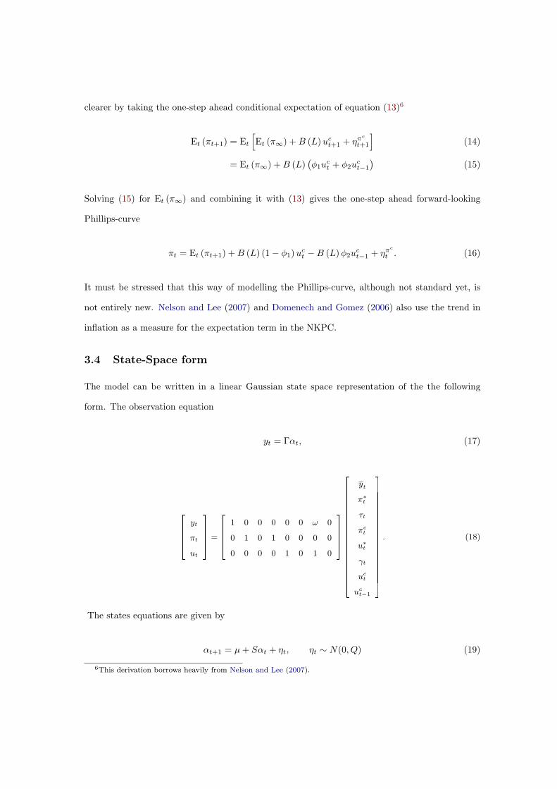
3.4 State-Space form

The model can be written in a linear Gaussian state space representation of the the following

form. The observation equation

yt = Γαt, (17)

26664

yt

πt

ut

37775 =

26664

1 0 0 0 0 0 ω 0

0 1 0 1 0 0 0 0

0 0 0 0 1 0 1 0

37775

26666666666666666664

yt

π∗t

τt

πct

u∗t

γt

uct

uct−1

37777777777777777775

. (18)

The states equations are given by

αt+1 = µ + Sαt + ηt, ηt ∼ N(0, Q) (19)

6This derivation borrows heavily from Nelson and Lee (2007).

26666666666666666664

yt+1

π∗t+1

τt+1

πct+1

u∗t+1

γt+1

uct+1

uct

37777777777777777775

=

26666666666666666664

µj

0

0

0

0

0

0

0

37777777777777777775

+

26666666666666666664

1 0 0 0 0 0 0 0

0 1 1 0 0 0 0 0

0 0 δ1 0 0 0 0 0

0 0 0 0 0 0 κ1 κ2

0 0 0 0 1 1 0 0

0 0 0 0 0 δ2 0 0

0 0 0 0 0 0 φ1 φ2

0 0 0 0 0 0 1 0

37777777777777777775

26666666666666666664

yt

π∗t

τt

πct

u∗t

γt

uct

uct−1

37777777777777777775

+

26666666666666666664

η1t

η2t

η3t

η4t

η5t

η6t

η7t

0

37777777777777777775

. (20)

The variance-covariance matrix of the state innovations is given by

Q =

26666666666666666664

σ2η1 0 0 0 0 0 ση1η7 0

0 σ2η2 0 ση2η4 ση2η5 0 0 0

0 0 σ2η3 0 0 0 0 0

0 ση2η4 0 σ2η4 0 0 ση4η7 0

0 ση2η5 0 0 σ2η5 0 ση5η7 0

0 0 0 0 0 σ2η6 0 0

ση1η7 0 0 ση4η7 ση5η7 0 σ2η7 0

0 0 0 0 0 0 0 0

37777777777777777775

. (21)

The likelihood for the linear Gaussian state space model can be calculated by a routine ap-

plication of the Kalman filter and maximised with respect to the unknown parameters using an

iterative numerical procedure (see e.g. Harvey, 1989; Durbin and Koopman, 2001). The station-

ary state variables are initialised by drawing from their stationary distributions while a diffuse

initialisation is used for the non-stationary state variables. Standard errors for the estimates are

calculated by inverting the Hessian matrix.

4 Estimation Results

4.1 Structural breaks on output growth

Table (1) presents the results of the BP tests on structural breaks in output growth.7 Both, the

WDmax and the UDmax test statistic clearly reject the null hypothesis of no structural breaks

in GDP growth at conventional confidence levels. The sequential analysis also rejects the null

of no breaks against the alternative hypothesis of one structural break. However more than one7The results of the BP tests have been obtained by using the original GAUSS program from P. Perron available

on his webpage.

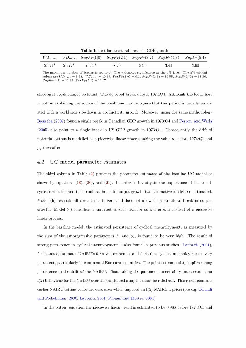
Table 1: Test for structural breaks in GDP growth

WDmax UDmax SupFT (1|0) SupFT (2|1) SupFT (3|2) SupFT (4|3) SupFT (5|4)

23.21* 25.77* 23.31* 8.29 3.99 3.61 3.90

The maximum number of breaks is set to 5. The ∗ denotes significance at the 5% level. The 5% criticalvalues are UDmax = 9.52, WDmax = 10.39, SupFT (1|0) = 9.1, SupFT (2|1) = 10.55, SupFT (3|2) = 11.36,SupFT (4|3) = 12.35, SupFT (5|4) = 12.97.

structural break cannot be found. The detected break date is 1974:Q1. Although the focus here

is not on explaining the source of the break one may recognise that this period is usually associ-

ated with a worldwide slowdown in productivity growth. Moreover, using the same methodology

Basistha (2007) found a single break in Canadian GDP growth in 1973:Q4 and Perron and Wada

(2005) also point to a single break in US GDP growth in 1973:Q1. Consequently the drift of

potential output is modelled as a piecewise linear process taking the value µ1 before 1974:Q1 and

µ2 thereafter.

4.2 UC model parameter estimates

The third column in Table (2) presents the parameter estimates of the baseline UC model as

shown by equations (18), (20), and (21). In order to investigate the importance of the trend-

cycle correlation and the structural break in output growth two alternative models are estimated.

Model (b) restricts all covariances to zero and does not allow for a structural break in output

growth. Model (c) considers a unit-root specification for output growth instead of a piecewise

linear process.

In the baseline model, the estimated persistence of cyclical unemployment, as measured by

the sum of the autoregressive parameters φ1 and φ2, is found to be very high. The result of

strong persistence in cyclical unemployment is also found in previous studies. Laubach (2001),

for instance, estimates NAIRU’s for seven economies and finds that cyclical unemployment is very

persistent, particularly in continental European countries. The point estimate of δ1 implies strong

persistence in the drift of the NAIRU. Thus, taking the parameter uncertainty into account, an

I(2) behaviour for the NAIRU over the considered sample cannot be ruled out. This result confirms

earlier NAIRU estimates for the euro area which imposed an I(2) NAIRU a priori (see e.g. Orlandi

and Pichelmann, 2000; Laubach, 2001; Fabiani and Mestre, 2004).

In the output equation the piecewise linear trend is estimated to be 0.986 before 1974Q:1 and

Table 2: Parameter Estimates

Baseline Model Model (b) Model (c)

Phillips curveση2 0.575 (0.087) 0.076 (0.108) 0.500 (0.072)

ση3 0.048 (0.657) 0.446 (0.139) 0.047 (0.291)

ση4 0.888 (0.068) 1.169 (0.093) 0.938 (0.017)

ση2η4 0.498 (0.082) - 0.468 (0.074)

ση2η5 -0.011 (0.014) - -0.002 (0.009)

κ1 -3.230 (1.366) -4.568 (1.550) -2.818 (1.031)

κ2 2.349 (1.293) 1.569 (1.166) 1.707 (1.066)

δ1 0.067 (0.107) -0.083 (0.096) 0.086 (0.091)

Unemploymentση5 0.089 (0.006) 0.066 (0.010) 0.087 (0.006)

ση6 0.011 (0.005) 0.050 (0.016) 0.010 (0.006)

ση7 0.050 (0.007) 0.065 (0.014) 0.058 (0.009)

ση5η7 0.000 (0.001) - -0.001 (0.001)

ση7η4 0.021 (0.015) - 0.022 (0.010)

φ1 1.893 (0.035) 1.672 (0.121) 1.886 (0.039)

φ2 -0.917 (0.035) -0.686 (0.130) -0.905 (0.039)

δ2 0.987 (0.013) 0.912 (0.052) 0.976 (0.013)

Outputση1 0.441 (0.032) 0.398 (0.049) 0.438 (0.031)

σηµ- - 0.011 (0.012)

ση1η7 -0.018 (0.004) - -0.017 (0.004)

ω -1.590 (0.366) -4.618(1.75) -1.932 (0.359)

µ1 0.986 (0.120) 0.601 (0.066)* -µ2 0.547 (0.041) - -

log-likelihood 8.911 -5.563 -2.480

Standard errors are in parentheses. Model (b) restricts all covariances to zero and does not allowfor a structural break in potential output growth. Model (c) specifies potential output growth as aunit-root process. * µ1 refers to potential output growth over the full sample.

0.547 thereafter which corresponds to an output growth rate of 3.94% respectively 2.19% p.a..

This sharp decrease highlights once again the need for a proper output growth specification. The

Okun’s Law parameter, ω, has the correct sign and a reasonable magnitude.8 Turning to inflation,

the slope of the Phillips-curve is found to be -0.881. At first sight, this might be surprising as

previous studies estimated this parameter to range from -0.7 to zero. However, the way of mod-

elling the Phillips curve here relies on a trend-cycle decomposition of inflation, implying that the

slope of the Phillips-curve is equal to the trade-off between the cyclical components of inflation

and unemployment. Using a similar specification of the Phillips-curve Nelson and Lee (2007)

8More dynamics in the Okun’s Law equation, i.e. a lagged impact of cyclical unemployment on the output gapwas found to be statistically insignificant.

estimated a slope of -0.9 for US data. The transitory dynamics around the trend in inflation are

not significant, implying a simple unit-root behaviour for the core inflation rate. The estimated

covariances not only ensures that the empirical model does not have unnecessary parameter re-

strictions, it also gives some economic insights. The covariance between the trend and cycle of the

rate of unemployment can be interpreted as a test for possible hysteresis effects. The term hys-

teresis, originally stemming from physics, refers to a situation in which transitory unemployment

translates into long-run unemployment. This idea has been introduced by Blanchard and Sum-

mers (1986) who argued hysteresis effects can arise from insider-outsider effects in wage formation.

However, the results here do not show hysteresis effects in the rate of unemployment. Moreover,

the covariance between shocks to the NAIRU and shocks to the core inflation rate are close to zero

and statistically insignificant. Thus there is no trade-off between inflation and unemployment in

the long-run as suggested by theory.

The parameter estimates of the two restricted alternative models show a somewhat mixed pic-

ture. In model (c), where trend output growth is a random walk process, the estimated parameters

are close to those from the baseline model. In model (b), however, the point estimates of some

parameters are not economically meaningful, e.g. the slope of the Phillips curve is estimated to

be -2.999. Moreover, the Okun’s Law parameter is found to be -4.618. A likelihood-ratio test

between the baseline model and model (b) shows that the baseline model outperforms model (b).

The test statistic of 28.948 which is distributed as chi-squared with six degrees of freedom leads

to the rejection of the restrictions imposed in model (b) at standard significance levels.9

4.3 State estimates

Figure (1) shows the smoothed estimated states of the baseline model and their 95% confidence

intervals together with the original data. The sharp increase in the rate of unemployment until

the mid80s is explained by movements of the NAIRU. Cyclical unemployment, although very

persistent, is rather small in magnitude. The output gap is symmetric to the unemployment gap

since they are linked to each other via Okun’s Law. The core inflation rate evolves smoothly,

and thus transitory inflation appears to be very volatile. Overall, the estimated natural rates and

the corresponding gaps are consistent with earlier studies mostly based on a backward-looking9Note that a comparison between the baseline model and model (c) is not possible with a standard likelihood-

ratio test as model (c) is a different model rather than a restricted model in which parameters are set to zero.

Phillips-curve (see e.g. Fabiani and Mestre, 2004). The shadowed area in the output gap graph

indicate recessions as defined by the CEPR.10 The estimated gap picks up the business cycle

turning points quite accurately. Particularly the beginning of recessions is almost similar dated.

10The CEPR dating committee labels the decline in GDP from 2001 onwards a prolonged pause in the growth ofeconomic activity rather than a recession but notes that this might be reversed as revised GDP statistics appear(see http://www.cepr.org/data/Dating/ for details).

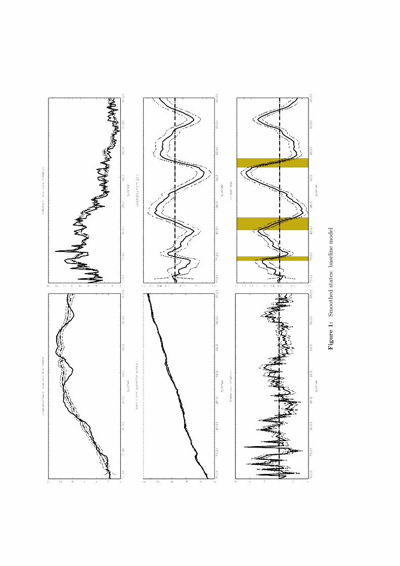
Fig

ure

1:

Sm

ooth

edst

ate

s:base

line

model

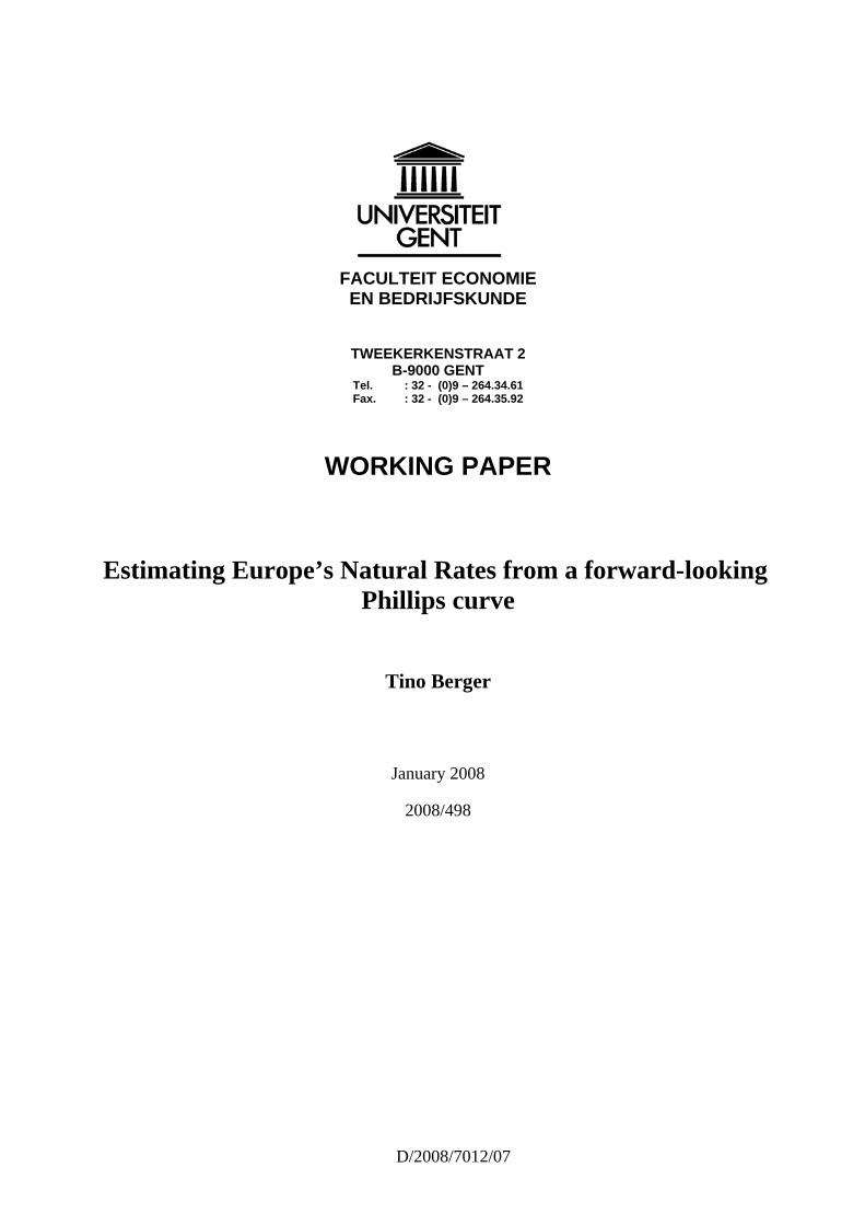
Figure (2) shows the trend in potential output for all three models. In model (b) this is a

constant taking the value 0.601 per quarter. To the contrary, the random walk trend captures

the sharp decrease in the early 70s but moves back to a level of around 0.8 at the end of the

70s. From then onwards it steadily decreases to approach µ2 at the end of the sample. Thus,

model (c) suggests that there was a sharp decrease in potential output growth at the beginning

of the sample. The increase of more than 1% in 1975:Q1 is quite surprising from an economic

perspective. However, if the true process is piecewise linear as in the baseline model, the random

walk trend with Gaussian error terms is not an adequate alternative. The innovations of such a

process with a single but large shift and only small changes before and after the break would not

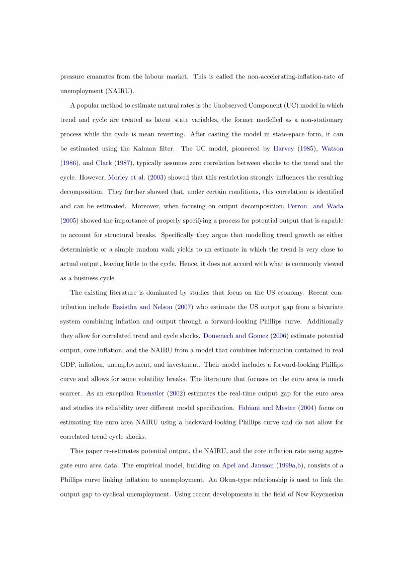
have a Gaussian distribution. Figure (3) shows the output gaps form the three models. Although

the timing of the turning points is very similar in all models they show a very different picture.

In model (b) actual output stays above potential output for the first half of the sample and below

it for almost the complete second half of the sample. Model (c) suggests that there was a positive

output gap of more than 3.5% around 1974. In the following years the output gap is close to zero,

a finding that is not confirmed by the baseline model which shows a positive output gap in second

half of the 70s.

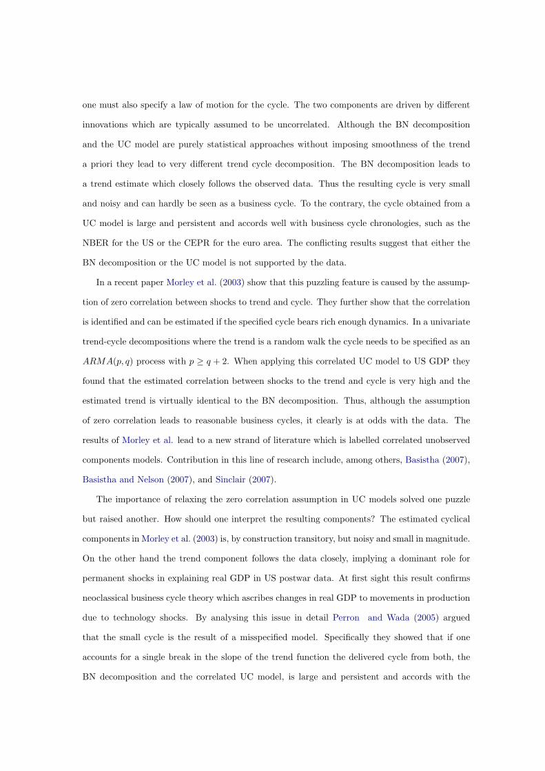
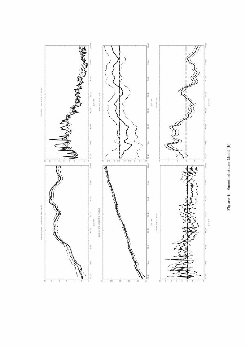
Figure (4) and (5) in the Appendix show the smoothed states estimates of the two alternative

models.

5 Conclusion

This paper re-estimates potential output, the NAIRU, the core inflation rate, and the corre-

sponding gaps for the euro area over the period 1970-2005. Output, inflation, and the rate of

unemployment are decomposed into a non-stationary and a stationary component. An Okun type

relation is used to link the output gap to the unemployment gap. In the Phillips curve, the core

inflation rate is used as a proxy for the forward-looking expectations term. Different from previous

studies in the field, the empirical model allows for large but infrequent shifts in the growth rate of

output. Moreover, accounting for recent advances in unobserved components models, the shocks

to the trend and the cyclical component of each series are allowed to be correlated. The results

show that that there is an one-time large shift in the growth rate of output in 1974:Q1. This

indicates that the conventional approach of modelling output growth as either deterministic or

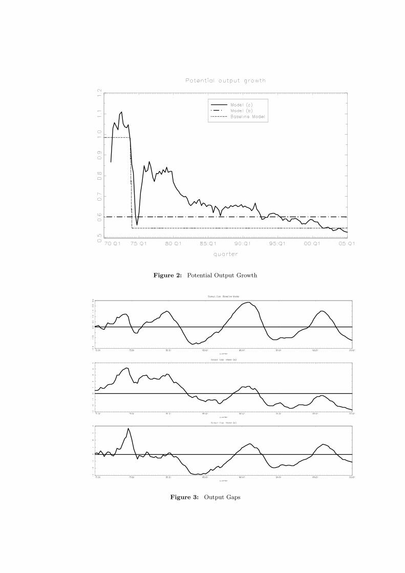
Figure 2: Potential Output Growth

Figure 3: Output Gaps

a unit-root process with shocks occurring every period is inadequate of capturing this shift. By

comparing the baseline model to an alternative model without a structural break and covariances

that are set to zero, it is shown that these restrictions are not supported by the data. On the other

hand, a model with a random walk drift in potential output suggests that after the large decrease

in output growth in the early 70s there was a sharp increase in output growth. This result is more

a statistical artifact as the shocks driving the unit-root trend are assumed to be Gaussian. Finally

the output gap of the baseline model is compared to the business cycle dating of the CEPR and

found to accord quite precisely with it.

References

Apel, M. and Jansson, P. (1999a). System estimates of potential output and the nairu. Empirical

Economics, 24(3):373–388.

Apel, M. and Jansson, P. (1999b). A theory-consistent system approach for estimating potential

output and the nairu. Economics Letters, 64(3):271–275.

Bai, J. and Perron, P. (1998). Estimating and testing linear models with multiple structural

changes. Econometrica, 66(1):47–78.

Bai, J. and Perron, P. (2001). Multiple Structural Changes Models: a Simulation Analysis. forth-

coming in Econometric Essays.

Bai, J. and Perron, P. (2003). Computation and analysis of multiple structural change models.

Journal of Applied Econometrics, 18(1):1–22.

Basistha, A. (2007). Trend-cycle correlation, drift break and the estimation of trend and cycle in

canadian gdp. Canadian Journal of Economics, 40(2):584–606.

Basistha, A. and Nelson, C. R. (2007). New measures of the output gap based on the forward-

looking new keynesian phillips curve. Journal of Monetary Economics, 54(2):498–511.

Baxter, M. and King, R. G. (1999). Measuring business cycles: Approximate band-pass filters for

economic time series. The Review of Economics and Statistics, 81(4):575–593.

Beveridge, S. and Nelson, C. R. (1981). A new approach to decomposition of economic time series

into permanent and transitory components with particular attention to measurement of the

‘business cycle’. Journal of Monetary Economics, 7(2):151–174.

Blanchard, O. and Summers, L. (1986). Hysteresis and the european unemployment problem.

NBER Macroeconomics Annual, 1:15–77.

Burns, A. and Mitchell, W. (1946). Measuring Business Cycles. NBER, New York.

Canova, F. (1998). Detrending and business cycle facts. Journal of Monetary Economics,

41(3):475–512.

Clark, P. K. (1987). The cyclical component of u.s. economic activity. The Quarterly Journal of

Economics, 102(4):797–814.

Domenech, R. and Gomez, V. (2006). Estimating potential output, core inflation, and the nairu

as latent variables. Journal of Business & Economic Statistics, 24(3):354–366.

Durbin, J. and Koopman, S. (2001). Time Series Analysis by State Space Methods. Oxford

University Press.

Fabiani, S. and Mestre, R. (2004). A system approach for measuring the euro area NAIRU.

Empirical Economics, 29:311–341.

Fagan, G., Henry, J., and Mestre, R. (2005). An area-wide model (awm) for the euro area.

Economic Modelling, 22:39–59.

Friedman, M. (1968). The role of monetary policy. The American Economic Review, 58:1–17.

Harvey, A. (1985). Trends and cycles in macroeconomic time series. Journal of Business and

Economic Statistics, 3:216–227.

Harvey, A. (1989). Forecasting structural time series models and the Kalman filter. Cambridge

University Press.

Hodrick, R. J. and Prescott, E. C. (1997). Postwar u.s. business cycles: An empirical investigation.

Journal of Money, Credit and Banking, 29(1):1–16.

Laubach, T. (2001). Measuring the nairu: Evidence from seven economies. The Review of Eco-

nomics and Statistics, 83(2):218–231.

Morley, J. C., Nelson, C. R., and Zivot, E. (2003). Why are the beveridge-nelson and unobserved-

components decompositions of gdp so different? The Review of Economics and Statistics,

85(2):235–243.

Nelson, C. R. and Lee, J. (2007). Expectation horizon and the phillips curve: the solution to an

empirical puzzle. Journal of Applied Econometrics, 22(1):161–178.

Okun, A. (1970). The Political Economy of Prosperity. Washington.

Orlandi, F. and Pichelmann, K. (2000). Disentangling trend and cycle in the eur-11 unemploy-

ment series. an unobserved component modelling approach. European Economy - Economic

Papers 140, Commission of the EC, Directorate-General for Economic and Financial Affairs

(DG ECFIN). available at http://ideas.repec.org/p/fth/eeccco/140.html.

Perron , P. and Wada, T. (2005). Let’s take a break: Trends and cycles in us real gdp? Boston

University - Department of Economics - Working Papers Series WP2005-031, Boston University -

Department of Economics. available at http://ideas.repec.org/p/bos/wpaper/wp2005-031.html.

Phelps, E. (1968). Money-wage dynamics and labor market equilibrium. Journal of Political

Economy, 76:678–711.

Proietti, T., Musso, A., and Westermann, T. (2007). Estimating potential output and the output

gap for the euro area: a model-based production function approach. Empirical Economics,

33:85–113.

Rapach, D. E. and Wohar, M. E. (2005). Regime changes in international real interest rates: Are

they a monetary phenomenon? Journal of Money, Credit and Banking, 37(5):887–906.

Roeger, W. (2006). The production function approach to calculating potential growth and output

gaps. estimates for eu member states and the us. Technical report, Workshop on Perspectives on

potential output and productivity growth, organised by Banque de France and Bank of Canada,

April 24 and 25, 2006.

Ruenstler, G. (2002). The information content of real-time output gap estimates: an appli-

cation to the euro area. Working Paper Series 182, European Central Bank. available at

http://ideas.repec.org/p/ecb/ecbwps/20020182.html.

Sinclair, T. (2007). Identifying the relationship between permanent and transitory movements in

u.s. output and the unemployment rate. Technical report, Washington University, unpublished.

Stock, J. and Watson, M. (1998). Median unbiased estimation of coefficient variance in a time-

varying parameter mode. Journal of the American Statistical Association, 93:349–358.

Watson, M. W. (1986). Univariate detrending methods with stochastic trends. Journal of Monetary

Economics, 18(1):49–75.

Appendices

Fig

ure

4:

Sm

ooth

edst

ate

s:M

odel

(b)

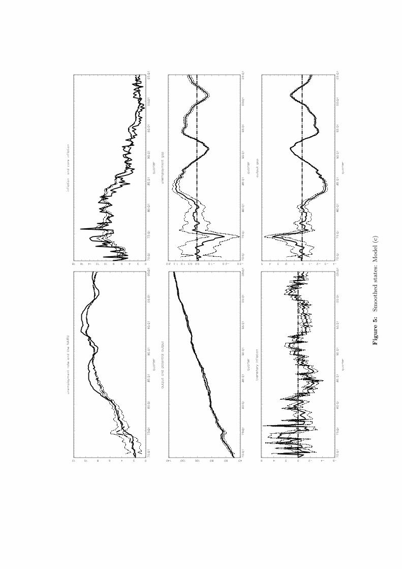
Fig

ure

5:

Sm

ooth

edst

ate

s:M

odel

(c)