Estimating Crop Yield Potential and Yield Gaps: From Field to Globe

Methods, approaches and innovations embodied in the Global Yield Gap and Water Productivity Atlas1

www.yieldgap.org

1 The Global Yield Gap and Water Productivity Atlas has been supported by funding from the University of Nebraska, Water for Food Institute (http://waterforfood.nebraska.edu/) and Wageningen UR, as well as by grants from the Bill and Melinda Gates Foundation and USAID through the Further Advancing the Blue Revolution program administered by Development Alternatives, Inc.

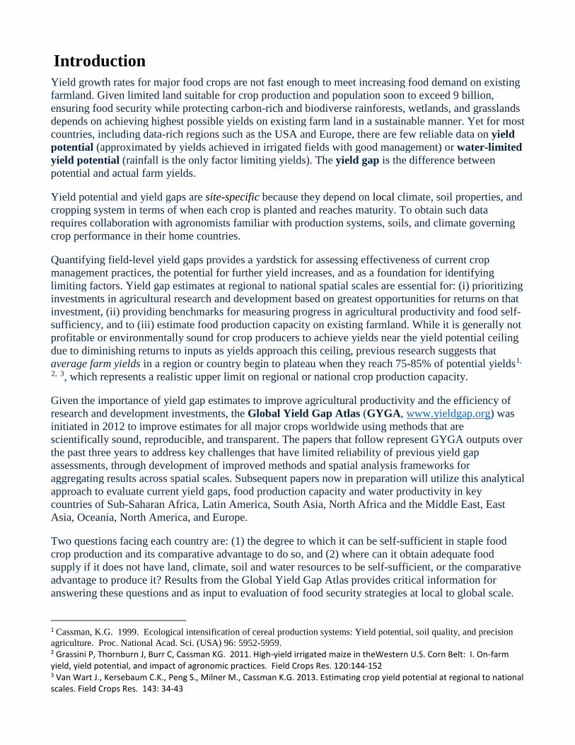
Introduction Yield growth rates for major food crops are not fast enough to meet increasing food demand on existing farmland. Given limited land suitable for crop production and population soon to exceed 9 billion, ensuring food security while protecting carbon-rich and biodiverse rainforests, wetlands, and grasslands depends on achieving highest possible yields on existing farm land in a sustainable manner. Yet for most countries, including data-rich regions such as the USA and Europe, there are few reliable data on yield potential (approximated by yields achieved in irrigated fields with good management) or water-limited yield potential (rainfall is the only factor limiting yields). The yield gap is the difference between potential and actual farm yields. Yield potential and yield gaps are site-specific because they depend on local climate, soil properties, and cropping system in terms of when each crop is planted and reaches maturity. To obtain such data requires collaboration with agronomists familiar with production systems, soils, and climate governing crop performance in their home countries. Quantifying field-level yield gaps provides a yardstick for assessing effectiveness of current crop management practices, the potential for further yield increases, and as a foundation for identifying limiting factors. Yield gap estimates at regional to national spatial scales are essential for: (i) prioritizing investments in agricultural research and development based on greatest opportunities for returns on that investment, (ii) providing benchmarks for measuring progress in agricultural productivity and food self-sufficiency, and to (iii) estimate food production capacity on existing farmland. While it is generally not profitable or environmentally sound for crop producers to achieve yields near the yield potential ceiling due to diminishing returns to inputs as yields approach this ceiling, previous research suggests that average farm yields in a region or country begin to plateau when they reach 75-85% of potential yields1, 2, 3, which represents a realistic upper limit on regional or national crop production capacity. Given the importance of yield gap estimates to improve agricultural productivity and the efficiency of research and development investments, the Global Yield Gap Atlas (GYGA, www.yieldgap.org) was initiated in 2012 to improve estimates for all major crops worldwide using methods that are scientifically sound, reproducible, and transparent. The papers that follow represent GYGA outputs over the past three years to address key challenges that have limited reliability of previous yield gap assessments, through development of improved methods and spatial analysis frameworks for aggregating results across spatial scales. Subsequent papers now in preparation will utilize this analytical approach to evaluate current yield gaps, food production capacity and water productivity in key countries of Sub-Saharan Africa, Latin America, South Asia, North Africa and the Middle East, East Asia, Oceania, North America, and Europe. Two questions facing each country are: (1) the degree to which it can be self-sufficient in staple food crop production and its comparative advantage to do so, and (2) where can it obtain adequate food supply if it does not have land, climate, soil and water resources to be self-sufficient, or the comparative advantage to produce it? Results from the Global Yield Gap Atlas provides critical information for answering these questions and as input to evaluation of food security strategies at local to global scale.

1 Cassman, K.G. 1999. Ecological intensification of cereal production systems: Yield potential, soil quality, and precision agriculture. Proc. National Acad. Sci. (USA) 96: 5952-5959. 2 Grassini P, Thornburn J, Burr C, Cassman KG. 2011. High-yield irrigated maize in theWestern U.S. Corn Belt: I. On-farm yield, yield potential, and impact of agronomic practices. Field Crops Res. 120:144-152 3 Van Wart J., Kersebaum C.K., Peng S., Milner M., Cassman K.G. 2013. Estimating crop yield potential at regional to national scales. Field Crops Res. 143: 34-43

GYGA Team Members Central Coordinating Team http://www.yieldgap.org/web/guest/main-partners University of Nebraska

Kenneth Cassman, Robert B. Daugherty Professor of Agronomy Patricio Grassini, Assistant Professor of Agronomy and Horticulture Haishun Yang, Associate Professor of Agronomy and Horticulture Justin van Wart, Post-Doctoral Research Associate of Agronomy and Horticulture Nicolas Guilpart, Post-Doctoral Research Associate of Agronomy and Horticulture

Wageningen University and Alterra

Martin van Ittersum, Professor of Plant Production Systems Lenny van Bussel, Post-Doctoral Research Associate Joost Wolf, Senior Researcher Hendrik Boogaard, Senior Scientist Hugo de Groot, Senior IT Developer

Regional Team Members http://www.yieldgap.org/web/guest/regional-partners

ICRISAT

Lieven Claessens, Senior Scientist

Africa Rice

Kazuki Saito, Agronomist Pepijn van Oort, Crop Modeler

Country Agronomists

South Asiahttp://www.yieldgap.org/web/guest/partners -asia

Jagadish Timsina, Bangladesh Nataraja Subash, India P.S. Brahmanand, India

Sub-Saharan Africahttp://www.yieldgap.org/web/guest/partne rs-sub-saharan-africa

Korodjouma Ouattara, Burkina Faso Kindie Tesfaye, Ethiopia Samuel Adjei-Nsiah, Ghana Ochieng Adimo, Kenya Mamoutou Kouressy, Mali Agali Alhassane, Niger Abdullahi Bala, Nigeria Joachim Makoi, Tanzania Kayuki Kaizzi, Uganda Regis Chikowo, Zambia

North Africa and the Middle Easthttp://www.yieldgap.org/web/guest/partners -asia

Muien Qaryouti, Jordan Said Ouattar, Morocco Haithem Bahri, Tunisia

Australia http://www.yieldgap.org/web/guest/partners-australia

Zvi Hochman, CSIRO David Gobbett, CSIRO

Brazil http://www.yieldgap.org/web/guest/partners-latin-america

Geraldo Martha, Embrapa Fabio Marin, Embrapa

Table of Contents

Yield gap analysis with local to global relevance-A review Martin K. van ittersum, Kenneth G. Cassman, Patricio Grassini, Joost Wolf, Pablo Tittonell, Zvi Hochman

2013, Field Crops Research, Volume 143: 4-17

http://www.sciencedirect.com/science/article/pii/S037842901200295X

Use of agro-climatic zones to upscale simulated crop yield potential Justin van Wart, Lenny G.J. van Bussel, Joost Wolf, Rachel Licker, Patricio Grassini, Andrew Nelson, Hendrik Boogaard, James Gerber, Nathaniel D. Mueller, Lieven Claessens, Martin K. van Ittersum, Kenneth G. Cassman

2013, Field Crops Research, Volume 143: 44-55

http://www.sciencedirect.com/science/article/pii/S0378429012004121#

Assessment of rice self-sufficiency in 2025 in eight African countries P.A.J. van Oort, K. Saito, A. Tanaka, E. Amovin-Assagba, L.G.J. Van Bussel, J. van Wart, H. de Groot, M.K. van Ittersum, K. G. Cassman, M.C.S. Wopereis

2015, Global Food Security, Volume 5: 39-49

http://www.sciencedirect.com/science/article/pii/S2211912415000036

How good is good enough? Data requirements for reliable crop yield simulations and yield-gap analysis Patricio Grassini, Lenny G.J. van Bussel, Justin van Wart, Joost Wolf, Lieven Claessens, Haishun Yang, Hendrik Boogaard, Hugo de Groot, Martin K. van Ittersum, Kenneth G. Cassman

2015, Field Crops Research, Volume 177: 49–63 http://www.sciencedirect.com/science/article/pii/S0378429015000866

From field to atlas: Upscaling of location-specific yield gap estimates Lenny G.J. van Bussel, Patricio Grassini, Justin van Wart, Joost Wolf, Lieven Claessens, Haishun Yang, Hendrik Boogaard, Hugo de Groot, Kazuki Saito, Kenneth G. Cassman, Martin K. van Ittersum

2015, Field Crops Research, Volume 177: 98–108

http://www.sciencedirect.com/science/article/pii/S0378429015000878

Creating long-term weather data from thin air for crop simulation modelling. Justin Van Wart, Patricio Grassini, Haishun Yang, Lieven Claessens, Andy Jarvis, Kenneth G. Cassman

2015, Agriculture and Forest Meteorology

Yield gap analysis with local to global relevance-A review

Martin K. van ittersum, Kenneth G. Cassman, Patricio Grassini, Joost Wolf, Pablo Tittonell, Zvi Hochman

2013, Field Crops Research, Volume 143: 4-17 http://www.sciencedirect.com/science/article/pii/S037842901200295X

Y

MJa

b

c

d

a

ARR1A

KFYWYBCC

1

fcndp2u

0h

Field Crops Research 143 (2013) 4–17

Contents lists available at SciVerse ScienceDirect

Field Crops Research

journa l homepage: www.e lsev ier .com/ locate / fc r

ield gap analysis with local to global relevance—A review

artin K. van Ittersum a,∗, Kenneth G. Cassman b, Patricio Grassini b,oost Wolf a, Pablo Tittonell c, Zvi Hochman d

Plant Production Systems group, Wageningen University, P.O. Box 430, 6700 AK Wageningen, The NetherlandsUniversity of Nebraska-Lincoln, P.O. Box 830915, Lincoln, NE 68583-0915, USAFarming Systems Ecology group, Wageningen University, P.O. Box 563, 6700 AN Wageningen, The NetherlandsCSIRO Ecosystem Sciences/Sustainable Agriculture Flagship, EcoSciences Precinct, 41 Boggo Road, Dutton Park, QLD 4102, Australia

r t i c l e i n f o

rticle history:eceived 27 April 2012eceived in revised form3 September 2012ccepted 16 September 2012

eywords:ood securityield potentialater-limited yield potential

ield gapsoundary functionrop simulation modelsropping system

a b s t r a c t

Yields of crops must increase substantially over the coming decades to keep pace with global food demanddriven by population and income growth. Ultimately global food production capacity will be limited bythe amount of land and water resources available and suitable for crop production, and by biophysicallimits on crop growth. Quantifying food production capacity on every hectare of current farmland ina consistent and transparent manner is needed to inform decisions on policy, research, developmentand investment that aim to affect future crop yield and land use, and to inform on-ground action bylocal farmers through their knowledge networks. Crop production capacity can be evaluated by estimat-ing potential yield and water-limited yield levels as benchmarks for crop production under, respectively,irrigated and rainfed conditions. The differences between these theoretical yield levels and actual farmers’yields define the yield gaps, and precise spatially explicit knowledge about these yield gaps is essential toguide sustainable intensification of agriculture. This paper reviews methods to estimate yield gaps, witha focus on the local-to-global relevance of outcomes. Empirical methods estimate yield potential from 90to 95th percentiles of farmers’ yields, maximum yields from experiment stations, growers’ yield contestsor boundary functions; these are compared with crop simulation of potential or water-limited yields.Comparisons utilize detailed data sets from western Kenya, Nebraska (USA) and Victoria (Australia). Wethen review global studies, often performed by non-agricultural scientists, aimed at yield and sometimesyield gap assessment and compare several studies in terms of outcomes for regions in Nebraska, Kenyaand The Netherlands. Based on our review we recommend key components for a yield gap assessmentthat can be applied at local to global scales. Given lack of data for some regions, the protocol recom-

mends use of a tiered approach with preferred use of crop growth simulation models applied to relativelyhomogenous climate zones for which measured weather data are available. Within such zones simula-tions are performed for the dominant soils and cropping systems considering current spatial distributionof crops. Need for accurate agronomic and current yield data together with calibrated and validated cropmodels and upscaling methods is emphasized. The bottom-up application of this global protocol allows

yield

verification of estimated

. Introduction

Whereas seven years ago there was relatively little concernor meeting projected food demand through improvements inrop productivity, today there is increasing awareness that “busi-ess as usual” will not allow food production to keep pace withemand—a situation that may result in dramatic rises in food prices,

overty, and hunger (FAO, 2003, 2006; Royal Society of London,009; Koning and van Ittersum, 2009; Godfray et al., 2010). Indeed,ntil recently, the most widely used computational equilibrium

∗ Corresponding author. Tel.: +31 317482382; fax: +31 317484892.E-mail address: martin.vanittersum@wur.nl (M.K. van Ittersum).

378-4290/$ – see front matter © 2012 Elsevier B.V. All rights reserved.ttp://dx.doi.org/10.1016/j.fcr.2012.09.009

gaps with on-farm data and experiments.© 2012 Elsevier B.V. All rights reserved.

models that evaluate global food supply and demand predicted thatgrain prices would remain constant or decrease in coming decades(Rosegrant et al., 1995, 2002; Colby et al., 1997; Cranfield et al.,1998; Rosegrant and Cline, 2003).

Three things are responsible for this remarkable turnaround inprognosis for global food security: (1) economic development ratesin the world’s most populous countries have consistently exceededprojections by a wide margin; (2) large increases in demand forenergy, grain, and livestock products in these countries due to arapid rise in purchasing power; and (3) global slowing of crop

yield rates of grain (Cassman et al., 2003, 2010; Steinfeld et al.,2006; Royal Society of London, 2009; Brisson et al., 2010; Fischerand Edmeades, 2010). It is now clear that during the next severaldecades, as human population rises towards a climax at 9 + billion,

d Crop

earyqflt

rffftocrtfmepi

ewmsstcticpri

byt11i(osdffiaSryiepl2

osyacm

M.K. van Ittersum et al. / Fiel

very hectare of existing crop land will need to produce yields thatre substantially greater than current yield levels. However, someegions have much greater potential than others to support higherields in a sustainable manner, due to their favourable climate, soiluality, and in some cases, access to irrigation. In some of these

avourable regions current average farm yields are low. Hence, aarge exploitable gap exists between current yields and what isheoretically achievable under ideal management.

Given the need for sustainable intensification, identifyingegions with greatest potential to increase food supply is criticalor four reasons. First, yield gap analysis provides the foundationor identifying the most important crop, and soil and managementactors limiting current farm yields and improved practices to closehe gap. Second, to enable effective prioritization of research, devel-pment, and interventions. Third is to evaluate impact of climatehange and other future scenarios that influence land and naturalesource use. And fourth, results from such analysis are key inputso economic models that assess food security and land use at dif-erent spatial scales. Computable general and partial equilibrium

odels typically rely on historical yield trends with some kind ofxtrapolation into the future. However, the agronomic basis of suchrojections and associated resource requirements can be much

mproved through rigorous yield gap analyses.For all these reasons, a geospatially explicit assessment of

xploitable gaps is required for the major food crops worldwideith local, agronomic relevance and with public access. And whileore detailed information about yield gaps is necessary, it is not

ufficient to fully inform research prioritization and investmenttrategies. Analyses of markets, policies, infrastructure and insti-utional factors are also needed. Without yield gap assessmentoupled with appropriate socio-economic analysis of constraintso improved productivity, policy makers and researchers will findt difficult to accurately assess future food security and land usehange. This in turn may lead to policy development and researchrioritization that are not well-informed, especially in developingegions such as Sub-Saharan Africa and South Asia where currentnformation is sparse.

The usefulness and rigor of yield gap analyses is demonstratedy various examples. Already in the 1960s, when average farmerields were below 5 Mg ha−1 in the Netherlands, it was computedhat wheat yields could exceed 10 Mg ha−1 (De Wit, 1959; Alberda,962). While few believed this could be true at that time, since993 average farmers’ yields in important wheat growing areas

n the Netherlands have regularly exceeded 9 or even 10 Mg ha−1

Centraal Bureau voor de Statistiek). In Australia, the early workf French and Schultz (1984) estimated water-limited yields andhowed that yields were limited by factors other than water,espite farmers’ perception that water was the single most limiting

actor. Recognition of these other limiting factors led to identi-cation of improved management practices such that yield gapsre now smaller (Hochman et al., 2012a,b). Yield gap analyses foroutheast Asia helped explain yield trends in irrigated rice andevealed that nitrogen management had to be improved to increaseields (Kropff et al., 1993). In Nebraska, recent yield gap analysis ofrrigated maize identified the recent plateauing of yields in farm-rs’ fields to be associated with a yield level about 85% of the yieldotential ceiling (Grassini et al., 2011a), which is similar to yield

evels at which other crops have plateaued (Cassman et al., 2003,010).

This review aims at comparing and assessing different meth-ds of yield gap analysis across spatial scales from the field, toub-national and national scales, to identify key components of

ield gap analysis that ensure adequate transparency, accuracy,nd reproducibility. In this paper we begin with definitions and aonceptual framework for agronomically relevant yield gap assess-ent, and then evaluate the strengths and limitations of previously

s Research 143 (2013) 4–17 5

published local and global yield gaps. Based on this analysis, weidentify the key components and associated uncertainties of aglobal protocol for yield gap analysis to produce locally relevantoutcomes that can be aggregated to regional or national estimates.

2. Concepts

Yield potential (Yp), also called potential yield, is the yieldof a crop cultivar when grown with water and nutrients non-limiting and biotic stress effectively controlled (Evans, 1993; VanIttersum and Rabbinge, 1997). When grown under conditions thatcan achieve Yp, crop growth rate is determined only by solar radia-tion, temperature, atmospheric CO2 and genetic traits that governlength of growing period (called cultivar or hybrid maturity) andlight interception by the crop canopy (e.g., canopy architecture).Potential yield is location specific because of the climate, but intheory not dependent on soil properties assuming that the requiredwater and nutrients can be added through management (which, ofcourse, is not practical or cost-effective in cases where major soilconstraints, such as salinity or physical barriers to root prolifera-tion, are difficult to overcome). Thus, in areas without major soilconstraints, Yp is the most relevant benchmark for irrigated sys-tems or systems in humid climates with adequate water supply toavoid water deficits. For rainfed crops, water-limited yield (Yw),equivalent to water-limited potential yield, is the most relevantbenchmark. For partially (supplementary) irrigated crops, both Ypand Yw may serve as useful benchmark. Definition of Yw is similarto Yp, but crop growth is also limited by water supply, and henceinfluenced by soil type (water holding capacity and rooting depth)and field topography (runoff).

Both Yp and Yw are calculated for optimum or recommendedsowing dates, planting density and cultivar (which determinesgrowing period to maturity). Sowing dates and cultivar maturityare specified to fit within the dominant cropping system becausethe cropping system “context” is critically important in dictatingfeasible growth duration, particularly in tropical and semi-tropicalenvironments where two or even three crops are produced eachyear on the same piece of land. Farmers attempt to maximize pro-duction and/or profit for the entire cropping system rather than theyield or profit of an individual crop. Likewise, where machinery andlabour are limiting or costly, achieving optimal sowing dates maynot be feasible for most farms. We therefore argue it is also rele-vant to calculate Yp and Yw for current average or median plantingdates in addition to optimal dates.

Average yield (Ya) is defined as the yield actually achieved in afarmer’s field. To represent variation in time and space in a definedgeographical region, it is defined as the average yield (in space andtime) achieved by farmers in the region under the most widely usedmanagement practices (sowing date, cultivar maturity, and plantdensity, nutrient management and crop protection). The numberof years utilized for estimating Ya must be a compromise betweenvariability in yields and the necessity to avoid confounding effectsof temporal yield trends due to technological or climate change (seeSection 4).

The yield gap (Yg) is the difference between Yp (irrigated crops),or Yw (rainfed crops) and actual yields (Ya). Water resources tosupport rainfed and irrigated agriculture also are under pressure,making water productivity (WP—the efficiency with which wateris converted to food) another critical benchmark of food productionand resource use efficiency (Bessembinder et al., 2005; Passioura,2006; Grassini et al., 2011b). Water productivity is defined as

the ratio between (grain) yield and seasonal water supply, whichincludes plant-available soil water at planting, in-season rainfall,and applied irrigation (irrigated crops) minus the residual plant-available water in the root zone at maturity.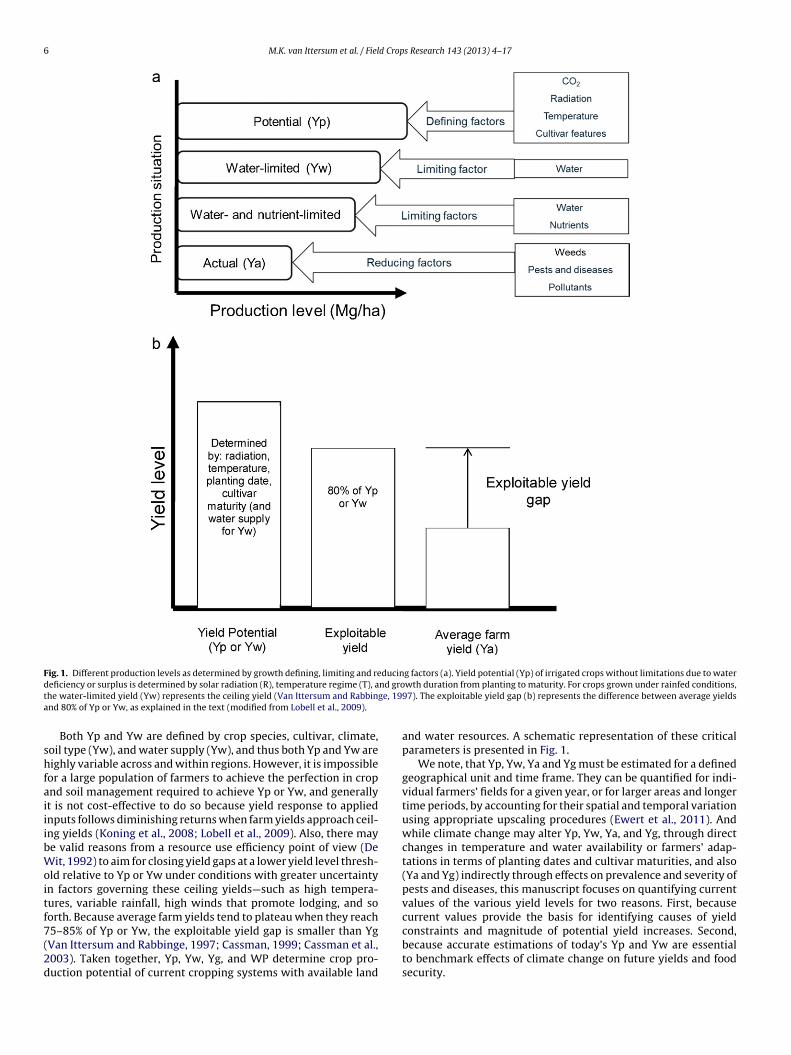

6 M.K. van Ittersum et al. / Field Crops Research 143 (2013) 4–17

Fig. 1. Different production levels as determined by growth defining, limiting and reducing factors (a). Yield potential (Yp) of irrigated crops without limitations due to waterd nd grot ge, 19a

shfaiiibWoitf7(2d

eficiency or surplus is determined by solar radiation (R), temperature regime (T), ahe water-limited yield (Yw) represents the ceiling yield (Van Ittersum and Rabbinnd 80% of Yp or Yw, as explained in the text (modified from Lobell et al., 2009).

Both Yp and Yw are defined by crop species, cultivar, climate,oil type (Yw), and water supply (Yw), and thus both Yp and Yw areighly variable across and within regions. However, it is impossible

or a large population of farmers to achieve the perfection in cropnd soil management required to achieve Yp or Yw, and generallyt is not cost-effective to do so because yield response to appliednputs follows diminishing returns when farm yields approach ceil-ng yields (Koning et al., 2008; Lobell et al., 2009). Also, there maye valid reasons from a resource use efficiency point of view (Deit, 1992) to aim for closing yield gaps at a lower yield level thresh-

ld relative to Yp or Yw under conditions with greater uncertaintyn factors governing these ceiling yields—such as high tempera-ures, variable rainfall, high winds that promote lodging, and soorth. Because average farm yields tend to plateau when they reach

5–85% of Yp or Yw, the exploitable yield gap is smaller than YgVan Ittersum and Rabbinge, 1997; Cassman, 1999; Cassman et al.,003). Taken together, Yp, Yw, Yg, and WP determine crop pro-uction potential of current cropping systems with available land

wth duration from planting to maturity. For crops grown under rainfed conditions,97). The exploitable yield gap (b) represents the difference between average yields

and water resources. A schematic representation of these criticalparameters is presented in Fig. 1.

We note, that Yp, Yw, Ya and Yg must be estimated for a definedgeographical unit and time frame. They can be quantified for indi-vidual farmers’ fields for a given year, or for larger areas and longertime periods, by accounting for their spatial and temporal variationusing appropriate upscaling procedures (Ewert et al., 2011). Andwhile climate change may alter Yp, Yw, Ya, and Yg, through directchanges in temperature and water availability or farmers’ adap-tations in terms of planting dates and cultivar maturities, and also(Ya and Yg) indirectly through effects on prevalence and severity ofpests and diseases, this manuscript focuses on quantifying currentvalues of the various yield levels for two reasons. First, becausecurrent values provide the basis for identifying causes of yield

constraints and magnitude of potential yield increases. Second,because accurate estimations of today’s Yp and Yw are essentialto benchmark effects of climate change on future yields and foodsecurity.

d Crop

3

aclttt

3

g(amfa

eoi(cYsolpauacb

p(pai(HHYoloeafitamrc

temppaDGa

M.K. van Ittersum et al. / Fiel

. Review of methods to assess yield gaps

Yield gaps have been estimated in previous studies with eitherglobal or local focus. Whereas global methods are generally

oarse and provide worldwide coverage using a consistent method,ocal studies are based on location-specific environmental condi-ions and management, which give local relevance but are hardo compare across locations and studies because of inconsistenterminology, concepts and methods.

.1. Local studies

At least four methods can be distinguished to estimate yieldaps at a local level (cf. Lobell et al., 2009): (1) field experiments,2) yield contests, (3) maximum farmer yields based on surveys,nd (4) crop model simulations. The first step associated with eachethod is to estimate yield ceilings as represented by Yp and Yw

or a given crop in a given location or region. Yg is then calculateds the difference between farmer’s Yp or Yw and Ya.

Although field experiments and yield contests can be used tostimate Yp and Yw for a given location and under a specific setf management practices, they require well-managed field studies

n which yield-limiting and yield-reducing factors are eliminatede.g., nutrient deficiencies, and diseases), and they must be repli-ated over many years to obtain a robust estimate of average Yp orw and their variation (Cassman et al., 2003). The latter may be aerious limitation in practice because it is difficult to avoid all abi-tic and biotic stresses and to do so consistently in a field study

asting several years. Also, in real-world farming, single crops areart of cropping and farming systems that often constrain sowingnd harvesting dates. Hence, field experiments and yield contestssed as a basis for estimating Yp or Yw must use sowing datesnd cultivar maturities that are representative of the prevailingropping systems in the region of interest if they are to serve asenchmarks for these systems.

Surveys among farmers to estimate maximum yields from upperercentiles represent another approach to estimate Yp or YwLobell et al., 2009). If crop production resources (including soilroperties) and input levels have also been recorded, methods suchs the boundary line approach or frontier analysis can be used todentify the highest yields for a given level of resource availabilityTittonell et al., 2008a; Fermont et al., 2009; Grassini et al., 2009;ochman et al., 2009; Wairegi et al., 2010; Hochman et al., 2012a).owever, if obstacles prevent all surveyed farmers from realizingp or Yw, then Yg will be underestimated. Such obstacles mustperate at the same scale as the yield gap analysis and could include

ack of access to inputs, lack of markets, and lack of knowledger access to it. While field experiments, yield contests and high-st yields obtained by farmers are useful to determine maximumchievable yields in a specific location or across a population ofelds (i.e., best genotype × environment × management interac-

ion, G × E × M), it is difficult to know for certain if all biotic andbiotic stresses were avoided. Therefore, yields from these sourcesay not be adequate to derive robust estimates of Yp or Yw rep-

esentative of the dominant weather and soil conditions in a givenropping system or region.

To overcome limitations of these approaches, crop simula-ion models can be used to estimate Yp or Yw (see e.g., Grassinit al., 2011a; Laborte et al., 2012). These simulation models areathematical representations of our current understanding of bio-

hysical crop processes (phenology, carbon assimilation, assimilateartitioning) and of crop responses to environmental factors (for

n overview of many crop growth models see Van Ittersum andonatelli, 2003). Such models have been designed to account for× E × M interactions. They require site-specific inputs, such

s daily weather data, crop management practices (sowing date,

s Research 143 (2013) 4–17 7

cultivar maturity, plant density), soil properties and specificationof initial conditions at sowing, such as soil water availability,and a model configuration that ensures nutrients to be non-limiting. Although specification of weather, soil, and managementpractices in current cropping systems is essential for robust sim-ulations of Yp and Yw, these data are typically not available formost cropping systems with adequate geospatial detail, even indeveloped countries. Also, models need to be rigorously eval-uated for their ability to reproduce measured yields of fieldcrops that received near-optimal management practices, acrossa wide a range of environments and management practices.Table 1 summarizes the key attributes of crop growth simulationmodels that we propose as desirable for use in yield gap assess-ment.

3.2. Comparison of methods to estimate yield gaps at local level

To assess possible implications of using different methods foryield gap assessment at a local level, we evaluated the follow-ing methods on their ability to estimate Yp (or Yw) and Yg acrossfarmer’s fields over relatively small geographic areas:

• site-specific simulation of Yp or Yw using crop growth models;• derivation of Yp or Yw from upper percentiles of farmer’s yield

distributions;• maximum yields measured in experimental stations, growers

contests, or highest-yielding farmer’s fields;• boundary-function analysis based on the relationship between

farmer’s yields and water supply.

These comparisons were performed for three cropping systemswith varying levels of intensification: rainfed maize in westernKenya, irrigated maize in Nebraska (USA), and rainfed wheat inVictoria (Australia). Underpinning data required to perform theseanalyses, including simulated Yp or Yw, actual yield and water sup-ply, were retrieved from previously published studies (Tittonellet al., 2008b; Hochman et al., 2009; Grassini et al., 2011a,b). Detaileddescriptions of cropping systems, crop models structure and vali-dation, and data inputs can be found in each study. In this example,information about yield, management, weather and soil propertieswere available for each farmer’s field from three years for Nebraskaand Victoria and one year for Kenya.

We argue crop simulation modelling is the most reliable way toestimate Yp or Yw and Yg in the context of a specific crop withina defined cropping system because these models can account forinteractions among weather, soils and management. Yp, Yw, andYg estimates based on simulation models are not single values,but rather probability distributions with a mean and range (Fig. 2).Variability in Yw and Yp reflects not only differences in manage-ment practices among fields, but also variability in weather andsoils across years and fields. Weather variability poses a dilemmafor farm managers who face large uncertainty about yield-affectingconditions in the season ahead, which in turn creates uncertaintyabout the most appropriate level of inputs. If they apply input lev-els in excess of amounts needed for maximum profit in a yearwhen Yp or Yw is below average due to unfavourable weather,they will likely achieve a small Yg but with smaller profit. On theother hand, if farmers invest too little inputs in a year with highYp or Yw due to favourable weather, they will miss the possi-bility of achieving a large profit and will have a large Yg. This isthe case for rainfed maize and wheat cropping system examplesin Kenya and Australia. However, an important distinction is that,

while Australian farmers face greater uncertainty about Yw, theyare also much better equipped to cope with this uncertainty, due tobetter access to information and inputs, than Kenyan farmers whooften also face labour constraints because of manual ploughing and

8 M.K. van Ittersum et al. / Field Crops Research 143 (2013) 4–17

Table 1Desired attributes of crop simulation models.

Desired attribute Explanation

Daily step simulation Simulation of daily crop growth and development based on weather, soil, and cropphysiological attributes

Flexibility to simulate managementpractices

Key management practices include: sowing date, plant density, cultivar maturity

Simulation of fundamental physiologicalprocesses

Simulation of key physiological processes such as crop development, net carbon assimilation,biomass partitioning, crop water relations, and grain growth

Crop specificity Should reflect crop-specific physiological attributes for respiration and photosynthesis, criticalstages and growth periods that define vegetative and grain filling periods, and canopyarchitecture

Minimum requirement of crop ‘genetic’coefficients

The model should have a low requirement of crop-site ‘genetic’ coefficients, preferably only alimited number of phenological coefficients

Validation against data from field cropsthat approach Yp and Yw

Comparison of model outcomes (grain yield, aboveground dry matter, cropevapotranspiration) against actual measured data from field crops that received managementpractices conducive to achieve Yp (irrigated) or Yw (rainfed crops)

User friendly Models embedded in user-friendly interfaces, where required data inputs and outputs can beeasily visualized, and with flexibility to modify default values for internal parameters

vailabcly ava

wi0ivt0

FtrHsc

Full documentation of modelparameterization and availability

Publicly aand publi

eeding. As a result, yield gaps are much smaller for rainfed wheatn Australia compared to rainfed maize in Kenya (Yg-to-Ya ratio of.4 and 2.2, respectively—Table 2). In the case of irrigated maize

n Nebraska, access to irrigation water compensates for weather

ariability and associated risk, allowing crop producers to optimizeheir farm management and achieve small Yg (Yg-to-Ya ratio of.1).

0

2

4

6

8

Gra

in y

ield

(M

g h

a-1

)

0

4

8

12

16

Field-ye0

2

4

6Yw = 2.4 Mg ha

-1 (CV=7

Yp= 14.7 Mg ha-1

(CV

Yw= 5.4 Mg ha-1

(CV=2Rainfed maize, west Kenya

Irrigated maize, Nebraska, USA

Rainfed wheat, Victoria,Australia

ig. 2. Simulated yield potential (Yp) or water-limited yield (Yw) based on site-specifichree cropping systems: rainfed maize in west Kenya, irrigated maize in Nebraska (USAespectively). Each bar corresponds to an individual field-year case. The yellow and red poorizontal lines indicate average Yp (or Yw) and Ya (solid and dashed lines, respectively)

hown. Fields were sorted from highest to lowest Yp or Yw. Note, that for the Victoria caseauses include incorrect specification of model inputs (management, soil/weather data), i

le models, published in the peer-review literature, with full documentationilable code, and with reference to data sources for internal parameter values

Empirical methods to estimate Yp, Yw, and Yg are generallybased on maximum yields or an upper yield percentile achievedby farmers, and are ‘static or non-spatially explicit’. As such theydo not reflect the full range of conditions within an agro-ecological

zone and cropping system (Fig. 3). The yield achieved by a con-test winner or in the highest-yielding fields in any region or seasonwas likely unattainable by most other farmers who did not benefit

ar number

0%); Ya = 1.7 Mg ha-1

(CV=77%); Yg = 0.8 Mg ha-1

(CV=95%)

=7%); Ya= 13.1 Mg ha-1

(CV=7%); Yg= 1.6 Mg ha-1

(CV=67%)

6%); Ya= 1.7 Mg ha-1

(CV= 56%); Yg= 3.7 Mg ha-1

(CV=36%)

Yw

Ya

Yw

Ya

Ya

Yp

weather, soil properties, and management data collected from farmer’s fields in), and rainfed wheat in Victoria (Australia) (n = 54, 123, and 129 field-year cases,rtion of the bars indicate actual farmer’s yield (Ya) and yield gap (Yg), respectively.for the region. Means and coefficients of variations (CV) for Yp (or Yw) and Yg are, actual yields are higher than simulated Yw for some of the site-years. Explanatoryncorrect reported yield, and model error in reproducing some particular G × E × M.

M.K. van Ittersum et al. / Field Crops Research 143 (2013) 4–17 9

Table 2Actual average farmer’s yield (Ya) and estimates of average yield potential (Yp) or water-limited yield (Yw), yield gaps (Yg), and Yg-to-Ya ratio (Yg:Ya) for three croppingsystems based on four different methods: crop simulation models, upper percentiles of farmer’s Ya, maximum yieldsa, and water-productivity boundary functions (seeFigs. 2–4). Values are means for one single year (rainfed maize in western Kenya) or 3 years for irrigated maize in Nebraska and rainfed wheat in Victoria.

Yield (Mg ha−1) Rainfed maize, western Kenya Irrigated maize, Nebraska, USA Rainfed wheat, Victoria, Australia

Actual yield (Ya) 1.7 13.2 1.9Yp or Yw based on: Yw Yp YwSimulation model 5.4 14.9 2.6

Upper percentiles Ya:95th percentile 3.6 14.4 3.599th percentile 3.9 14.8 4.1Maximum Yaa 6.0 17.6 4.3Boundary functions 13.0 15.4 3.3

Yg in Mg ha−1 (or as Yg:Ya ratio), based onb:Simulation model 3.7 (Yg:Ya = 2.2) 1.6 (Yg:Ya = 0.1) 0.8 (Yg:Ya = 0.4)

Upper percentiles Ya:95th percentile 1.9 (Yg:Ya = 1.1) 1.1 (Yg:Ya = 0.1) 1.9 (Yg:Ya = 1.0)99th percentile 2.2 (Yg:Ya = 1.3) 1.6 (Yg:Ya = 0.1) 2.2 (Yg:Ya = 1.2)Maximum Yaa 4.3 (Yg:Ya = 2.5) 4.5 (Yg:Ya = 0.3) 2.3 (Yg:Ya = 1.2)Boundary functions 11.3 (Yg:Ya = 6.6) 2.2 (Yg:Ya = 0.2) 1.4 (Yg:Ya = 0.8)

statioc est-y

fio(fipclanmsfig

Ft9maesas(tK

a Maximum yields were derived from measured yields at: nearby experimentalontest-winning irrigated fields in Nebraska (irrigated maize in Nebraska), and high

b For Australia, in few observations, Ya > Yw; then we assumed Yg = 0.0.

rom the same climatic or soil conditions. Likewise, measured yieldsn experimental stations can also be biased as these stations areften situated on the most fertile soils with favourable topographyi.e., flat land or on well terraced slopes, with deep soil pro-les), which can make them poorly representative of surroundingroduction systems. Hence, maximum yields and upper yield per-entiles provide an estimate of the best G × E interaction across aarge population of site-years, rather than a measure of long-termverage Yp or Yw. Although all these empirical methods are conve-ient when data are lacking to calibrate and validate a robust cropodel and to run it for a range of fields and years, they give incon-

istent estimates of Yp, Yw, and Yg compared to those obtained

rom crop simulation (Table 2). In the case where Ya is high, whichndicates favourable growing conditions and little stress (i.e., irri-ated maize in Nebraska) there is relatively close agreement among

ig. 3. Box plots showing distribution of actual farmer’s yields in three cropping sys-ems (box indicates 25th, 50th, and 75th percentiles; error bars indicate 10th and0th percentiles; solid circles indicate 5th and 95th percentiles). Arrows show esti-ates of Yp (irrigated maize in central USA) or Yw (rainfed maize in western Kenya

nd rainfed wheat in Australia) based on different methods: (i) crop simulation mod-ls (CSM) based on field-specific actual data on management practices, weather, andoil properties; (ii) 95th and 99th percentiles (P95 and P99, respectively) from thectual-yield distribution; (iii) maximum yields (MY) measured in nearby researchtation (western Kenya), farmers’ contests (USA), or farmer’s fields (Australia), andiv) boundary-functions (BF) for water productivity. Estimations of Yp or Yw withhe different methods are averages for one single year (rainfed maize in westernenya) or three years (irrigated maize in USA and rainfed wheat in Australia).

ns (rainfed maize in western Kenya), National Corn Growers Association (NCGA)ielding farmer field (rainfed wheat in Victoria).

Yp, Yw, and Yg estimates based on maximum yields or upper per-centiles and estimates based on crop simulation. In contrast, there isvery poor agreement among these estimates in cases where farmersdo not (or cannot) use best management practices and thus achievelow yields (i.e., Kenya rainfed maize). Likewise, estimates of Yp orYw based on maximum yield or upper percentiles can be heavilybiased if there are atypical years or farms amongst the observa-tions, and there is no way of knowing if this is the case withouta more detailed analysis using simulation models. This problemplays a role in the dataset for rainfed wheat in Victoria in which theaverage maximum yield and the average 95 and 99 percentiles offarmer’s yields across three years is well above the average simu-lated water-limited yield over the same period (Fig. 3). If we hadtaken the maximum yield and 95 and 99 percentiles of farmer’syields while lumping the three years, this difference would be sub-stantially higher as the best year is now used as the benchmark(data not shown).

Boundary functions based on the relationship between actualyields and water supply (or another limiting factor) can be con-sidered as a reasonable approach to estimate Yp and Yg whencrop simulation models and required data inputs are not avail-able (Fig. 4). Major limitation in using boundary functions arisesfrom not accounting for factors that cause variation in Yw at thesame level of water supply such as distribution of rainfall relative tocrop growth stage, and variation in solar radiation and temperature.However, a major strength of this approach is that estimates of Yware not “static or non-spatially explicit” values like those derivedfrom upper yield percentiles or maximum yields. Instead, boundaryfunctions provide estimates of Yw across a wide range of water sup-ply, and Yg can be estimated for any field-year observation as thedifference between actual farmer’s yield and Yw derived from theboundary function at the same level of water supply. Furthermore,use of a boundary function may help to determine the presence oflimiting factors other than water supply (French and Schultz, 1984;Grassini et al., 2009; Hochman et al., 2009). For example, Fig. 4 con-trasts irrigated maize in Nebraska (rarely water-limited and closeto Yp) with rainfed wheat in Australia (mostly water-limited andclose to the boundary) on one hand, versus, rainfed maize in Kenya(presumably less water-limited but still far from the boundary)

on the other. According to the boundary function water-limitedmaize yields in western Kenya and Nebraska are comparable (13.0and 15.4 Mg ha−1, respectively), but average Ya of rainfed maize inKenya is 87% lower than irrigated maize yield in Nebraska due to

10 M.K. van Ittersum et al. / Field Crop

Water supply (mm)

0 250 500 750 1000 1250

Gra

in y

ield

(M

g h

a-1

)

0

3

6

9

12

15

18

Rainfed ma ize, West Kenya

Irr iga ted ma ize, Nebraska (USA)

Rainfed wheat, Victoria (Australia)

201 mm651 mm

919 mm

Fig. 4. Actual farmer’s yields plotted against water supply. Data were collected fromfarmers’ fields in three cropping systems. Water supply includes plant available soilwater at planting plus in-season water inputs from rainfall and irrigation. Estimatedsurface runoff was subtracted from the estimate of water supply for rainfed maizein Kenya to reflect the actual lower crop water availability due to steep terrain. Aboundary function for cereal crops water productivity is shown (solid line), withx-intercept and slope equal to 60 mm and 22 kg ha mm−1, respectively (Sadras andAngus, 2006) and an upper yield limit of 15.4 Mg ha−1 at water supply ≥800 mm,established based on highest irrigated maize yields in Nebraska. Average watersupply for each cropping system is indicated with arrows. Note, that one bound-ary function for wheat and maize is assumed. This is justified as there is not toomuch difference in water use efficiency (WUE) among C3 and C4 crops when com-parisons are based on the actual vapour pressure deficits (VPD) of the environmentswhere these crops are typically grown. The difference on WUE between C3 and C4that would be expected due to the difference in the photosynthetic pathway canosr

rlt

3

gdgcFethaTbarrfdysgpdgys

nly be observed when both types of crops are grown under similar VPD regime,omething possible in a greenhouse experiment, but not too common to find in theeal world.

ainfall distribution and other limitations such as poor soil fertility,ack of inputs, labour, and knowledge and information about howo deal with these limitations.

.3. Global studies

Global studies generally use empirical, statistical approaches oreneric crop growth models and a grid-based approach using globalatasets on climate, soils and sometimes agricultural land use andeneral crop calendars (Appendix A). The statistical methods takeurrent highest yields within a defined climatic zone (based on e.g.,AO statistics and Monfreda et al., 2008; Licker et al., 2010; Foleyt al., 2011; Mueller et al., 2012) or use a stochastic frontier produc-ion function (Neumann et al., 2010). They do not verify whetherighest yields accurately represent the biophysical Yp or Yw limits confirmed by either a robust simulation model or field studies.he major limitation of this method is that it does not distinguishetween irrigated and rainfed crops; thus, many Yg estimates forgiven climatic zone are based on irrigated crop yields—even in

egions where the crop in question is grown almost entirely underainfed conditions. Also, these studies do not explicitly accountor differences in crop Yp or Yw within cropping systems thatiffer in crop rotation or even the number of crops produced eachear. Global studies using generic crop growth models utilize aingle crop model to simulate generic crop yields for the entirelobe. Generally, the papers in which this approach is used do notrovide enough information on model calibration and evaluation to

etermine how robust the estimates are. Often global studies usingeneric crop growth models do not have the explicit aim to estimateield gaps; sometimes they aimed at estimating current yields andensitivities of these yields to variations in management or climate

s Research 143 (2013) 4–17

(Appendix A) (Stehfest et al., 2007; Liu et al., 2007; Deryng et al.,2011).

Studies to estimate Yp, Yw or Ya at global scales using cropsimulation models have been based on weather data with sub-optimal temporal or spatial resolution and/or without all necessaryweather variables required for accurate simulation of crop perfor-mance. For example, most of the studies included in Appendix Aused derived climate data interpolated into grids. The interpola-tion process adds uncertainty into crop simulation for a specificregion because the weather data used may not represent the actualweather accurately within the grid. However, a main advantage isthat it provides a framework for up-scaling and complete terres-trial coverage. The latter is much more difficult using a point-basedapproach that requires actual data for weather, soils and crop man-agement. A recent study found that gridded-interpolated weatherdata give estimates of Yp and Yw that may be considerably differ-ent than those obtained from point-based estimates using actualweather data from representative weather stations within the grid(Van Wart, 2011).

Another limitation of published global studies is that esti-mates of Yp, Yw, and Yg may not represent current managementof a cropping system (e.g., crop rotation, planting date, cultivarmaturity), which limits agronomic relevance (Appendix A). Forexample, to estimate Yp and Yw of maize for each major maize-producing country, Nelson et al. (2010) assumed that cultivars hadthe same maturity in all countries. Actual yields used to estimateYg are generally based on yields reported in FAOSTAT (FAO, 2012a)and the Agro-MAPS project, a collaboration between FAO, IFPRI(International Food Policy Research Institute), SAGE (Centre forSustainability and the Global Environment) and CIAT (The Inter-national Centre for Tropical Agriculture) (FAO, 2012b). These sameactual yield datasets also served as the basis for the crop area dis-tribution maps of Monfreda et al. (2008) that utilized data fromsubnational levels, where available, and otherwise used nationallevel data from FAOSTAT. Such spatially coarse statistical data onYa, when combined with more spatially granular weather and soildata, are likely to be an equally important source of error and uncer-tainty in estimating yield gaps as is uncertainty in the estimationof Yp or Yw.

3.4. Comparing local outcomes of global studies

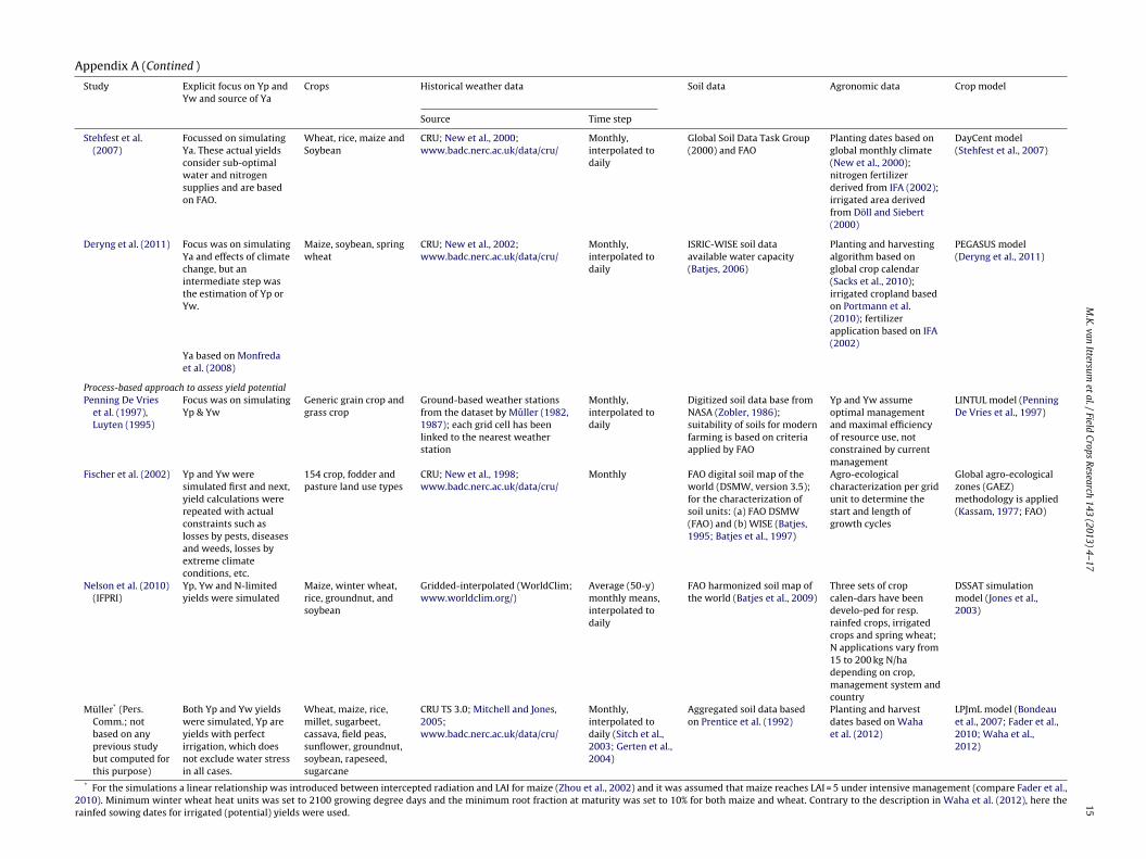
To assess whether alternative global studies using differentmethods result in different Yp or Yw and hence yield gaps for spe-cific regions, we asked scientists of published global yield studiesto share their data of the grids covering Nebraska (USA), Kenya(maize only) and The Netherlands (wheat only). Table 3 com-pares data from five studies for which methodological details areprovided in Appendix A. This comparison reveals how distinctthese studies are in aims, methods and results, whereas at a firstglance they may look rather similar. These differences also makecomparison of results from such studies difficult and sometimesnot justified. Since Stehfest et al. (2007) focused on simulationof nutrient-limited yields as a proxy for actual yields, results ofthis study for Kenya tell little about Yp or Yw. For Nebraska andThe Netherlands, where fertilizer application rates are high, sim-ulated nutrient-limited yields will in theory come close to Yp orYw. From Deryng et al. (2011) we obtained Yp and Yw for all threecountries, but spring wheat was simulated, which is not represen-tative for Nebraska and The Netherlands where winter wheat isgrown. Licker et al. (2010) and Neumann et al. (2010) did not dis-criminate between Yp and Yw—just one value for maximum yield

has been estimated. Spatially, Stehfest et al. (2007), Deryng et al.(2011), unpublished results with the LPJmL model (Bondeau et al.,2007; Ch. Müller, Potsdam Institute for Climate Impact Research,Germany) and Licker et al. (2010) did their calculations for all grid

M.K. van Ittersum et al. / Field Crops Research 143 (2013) 4–17 11

Table 3A comparison of Yp and Yw (Mg dry matter/ha) of five global yield studies of maize and wheat for Nebraska, Kenya and The Netherlands; Ya based on Monfreda et al. (2008)is provided in the last column. Averages for Kenya and The Netherlands across the grid cells are not weighted for crop area.

Latitude * longitude Stehfest et al.(2007)

Deryng et al.(2011)

Müller (2012, seeAppendix A)

Licker et al. (2010) Neumann et al. (2010) Monfreda et al. (2008)

Yp Yw Yp Yw Yp Yw Yp or Yw Yp or Yw Ya

Nebraska-maize40.5–41.0◦N; 101.5–102.0◦W 10.2 3.1 11.6 6.1 8.1 3.3 8.0 9.4 8.540.5–41.0◦N; 97.0–97.5◦W 9.7 5.4 11.3 10.1 8.1 5.9 9.0 9.2 7.942.0–42.5◦N; 97.0–97.5◦W 10.3 5.5 11.6 8.9 7.9 6.7 9.1 8.7 6.441.0–41.5◦N; 99–99.5◦W 9.9 5.2 12.9 9.1 8.1 5.1 9.2 10.1 8.041.0–41.5◦N; 96.0–96.5◦W 9.7 7.7 10.9 10.3 7.9 6.6 9.0 8.4 6.640.0–40.5◦N; 100.5–101.0◦W; 10.1 4.0 11.3 7.2 8.1 3.4 8.0 9.1 7.040.0–40.5◦N; 99.0–99.5◦W 9.8 4.6 11.8 9.3 8.2 4.7 9.2 10.1 8.6

Nebraska-wheat40.5–41.0◦N; 101.5–102.0◦W 4.2 0.9 9.7 6.8 11.2 6.6 3.1 3.5 2.340.0–40.5◦N; 100.5–101.0◦W; 4.1 1.0 9.8 7.8 11.3 7.5 3.1 4.7 2.640.0–40.5◦N; 99.0–99.5◦W 4.2 2.1 10.5 9.1 10.9 8.5 7.2 4.6 2.7

Kenya-maize Na 1.8 9.1 6.3 6.2 3.6 3.4 5.1 1.58.3

N grid o

cNgag(msaaa

aeettszYfiws

onspgaaMocr

4w

4

e

The Netherlands-wheat 9.5 9.8 6.2 5.4 8.9

a: Not available because the crop (irrigated or rainfed) is not very common in that

ells although size of grid cells differed among the studies, whereaseumann et al. (2010) took a 10% sample of all cropped 5′ × 5′

rids to allow for efficient statistical estimations and reduce spatialutocorrelation. Hence for the latter study, averages of the sampledrids were used for the national average, but for some countriese.g., The Netherlands) no grids were sampled and hence no esti-

ation of the Yp or Yw is available. All these differences betweentudies motivated a focus on the Nebraska data for a more completenalysis, while for Kenya and The Netherlands (non-weighted)verages per country are provided for the major croppingreas.

For Nebraska, average benchmarks for Yp vary between ca. 8nd almost 12 Mg ha−1 (maize) and ca. 4 up to 11 Mg ha−1 (wheat);ffects of water-limitation also strongly differ between the Stehfestt al., Deryng et al. and Müller studies (Table 3). It is not surprisinghat Licker et al. and Neumann et al. conclude a lower yield poten-ial than studies based on crop simulation models, as the statisticaltudies base their estimations on actual (average) farmers yields inones with similar conditions. In low-input crops or climate zones,p or Yw will be underestimated by definition. For Kenya, the dif-

erent studies lead to very different conclusions as to benchmarkingrrigated and rainfed maize production. Calculated benchmarks for

heat in The Netherlands also differed substantially between thetudies.

As indicated, the studies each had their own aim and meth-ds and differences in estimated Yp or Yw between the five doot tell which study is more valid or accurate; each of themerves its stated purpose at a global level. However, our com-arative analysis of local level methods indicates that existinglobal studies are encumbered with methodological assumptionsnd large uncertainties in data that prevents them from being

reliable source for location-specific of yield gap estimates.ethodologically, some studies do not allow the determination

f yield potential, while all lack the spatial and temporal pre-ision of input data which are required for local accuracy andelevance.

. Recommendations for a yield gap assessment protocolith local to global relevance

.1. Need for a bottom up approach to be locally relevant

As demonstrated in Section 3, existing methods lead to differentstimates of Yp and Yw, and therefore to differences in conclusions

6.3 Na 7.1

r country or no sample grids were available.

about magnitude and spatial distribution of Yg. We argue for atransparent, robust and reproducible protocol to estimate yieldgaps with local to global relevance. The protocol should be appliedconsistently across locations and crops in a “bottom-up” approachthat optimally exploits local knowledge and data. Global datasetson agricultural management (e.g., Waha et al., 2012) and actualyields (Monfreda et al., 2008) are generally too coarse for localrelevance. To allow for regional and global coverage of yield gapassessments there are basically two methods. First, a representa-tive point- or polygon-based approach estimates Yp, Yw, Ya and Ygfor selected points or polygons using observed input data and thenscales up to higher geographical units. This method assumes thatobserved or measured weather, soil, yields and cropping systemsdata are representative for the points or polygons. Second, a grid-based approach (generally used in global studies) uses inter- orextrapolated, gridded, weather, soil and cropping systems data tocalculate Yp, Yw (and possibly Ya itself); the outcomes of grids arethen upscaled to higher units. We postulate that the first methodhas the advantage that it is based on local observations and thatoutcomes of Yp, Yw, Ya and Yg can be verified on-the-ground morereadily than for the second method. This allows for a more agro-nomically relevant estimation of the yield gaps and identificationof factors limiting current farm yields. It remains to be investigatedwhich of the two scaling methods (cf. Ewert et al., 2011) leads tothe best estimation of yield gaps at larger units, such as provinces,states or nations.

4.2. Estimation of Yp or Yw

Based on Section 3.2 we conclude that simulation mod-els allow for the most reliable estimation of Yp, Yw and Ygbecause they: (i) account for variation in weather across yearsand regions, (ii) account for major interactions among crops,weather, soils, water regime and management, and (iii) allowquantification of potential or water-limited productivity withinthe climatic, soil and management context of a given croppingsystem. As such, crop models provide the means to capture spa-tial and temporal variation, to the extent that data are locationspecific, while this is not possible with any of the empiricalmethods (record yields, statistical yield distributions or high-

est yield within a defined agroclimactic or agro-environmentalzone).

We propose a number of criteria for selection of an appropri-ate crop growth simulation model (Table 1). Consistent with a

1 d Crop

bghll(gettdauo

4

lAstMtofaiaeahs

gNfvoccacflegcc

4

wtrsaoamgacd

2 M.K. van Ittersum et al. / Fiel

ottom-up approach, we argue that rather than using a singleeneric model globally, it is more important that a particular modelas been calibrated and evaluated for the conditions to be simu-

ated. Thus, models may differ per location, continent or crop, asong as the models have been validated under those conditionscf. Fig. 3). Large differences in estimates of Yp and Yw from thelobal studies (Table 3) make it clear that results from generic mod-ls need local validation to determine if estimates are accurate. Inerms of yield gap analysis, model inter-comparisons, such as inhe AgMIP project (Rosenzweig et al., in press), can shed light onifferences in performance of models for specific locations, if datare available for those locations of studies in which crops are grownnder a crop and soil management regime that allows expressionf Yp or Yw.

.3. Estimation of Ya

The accuracy of estimating Yg is determined by the weakestink, which perhaps in many cases may be the actual yields (Ya).ccurate geospatial distribution of current crop yields and theirpatial-temporal variability are needed, preferably more granularhan the FAO data or global datasets based on FAO data (such as

onfreda et al., 2008; You et al., 2009), that use national or some-imes provincial or state-wide averages. More detailed informationn actual farmers’ yields for specific locations can be based onarmers’ surveys and data from wholesale buyers. Some projectsre currently underway to achieve this greater spatial granular-ty, such as Global Futures (http://globalfuturesproject.com/) and

number of household panel survey datasets in progress at sev-ral international agricultural research centers. Expert knowledgend simple analysis (e.g., relating Ya to local rainfall) may alreadyelp to improve existing aggregated statistics of Ya at national orub-national levels.

In favourable, high yield environments, such as for irri-ated maize (Nebraska) and rainfed wheat production in Theetherlands, using yields of the 5 most recent years is adequate

or estimates of average yield with relatively low coefficient ofariation (CV), as 5 years’ averages are similar to estimates basedn the last 10 years’ (Fig. 5). In harsh environments for rainfedrop production, longer time intervals must be considered, and aompromise must be found between adequately capturing vari-bility on the one hand and avoiding the inclusion of technologicalhange (possibly including climate change) on the other hand. So,or Nebraska an average of 10 years is needed, as using fewer yearseads to biased estimates of average yield and CV due to the influ-nce of years with exceptionally high or low rainfall during the croprowing season, while longer time intervals include technologi-al change. For the Australian case 15–20 years may be a suitableompromise.

.4. Data and upscaling

The minimum data to estimate Yp and Yw include data oneather (daily time-step Tmax, Tmin, precipitation, solar radia-

ion, relative humidity and possibly windspeed), soil (in particularoot zone water holding capacity and runoff as determined byoil texture, soil depth and slope) and cropping systems (actualnd optimal sowing and harvesting dates, cultivar maturity, andptimum plant population density). We propose to use localgronomic information obtained from literature, surveys, govern-ent agencies, international institutions, or experts. Increasingly

lobal databases with sowing and harvesting dates are becomingvailable (e.g., Bondeau et al., 2007; Waha et al., 2012), and thesean eventually be used as a substitute, but only if local, observedata are not available.

s Research 143 (2013) 4–17

We also argue for use of daily observations of the weather;various authors have demonstrated that interpolated monthlyobservations may lead to overestimations of simulated yields inparticular in locations with high day-to-day variability in weatherconditions (Nonhebel, 1994; Soltani et al., 2004; Van Bussel et al.,2011). Weather data should be quality controlled and preferablyhave a time series of >15 years (Van Wart et al., 2013a). If measuredsolar radiation is not available (which is often the case) then thesecan be based on data from the NASA agroclimatology solar radiationdata (Bai et al., 2010; Van Wart et al., 2013b). If time series of >15years observed weather data are not available, such series could begenerated from shorter periods of observed data with additionalcalibration sources, or if no observed data are available, gridded,generated weather data may need to be used.

Assuming the choice for a point or polygon-based approachand observed data (as opposed to generated or interpolated data),we recommend use of spatial maps of crop areas (e.g., the MIRCAdataset of Portmann et al., 2010, the SPAM dataset of You et al., 2009or more refined national maps) as a reference to identify importantpoints or polygons for which Yg must be estimated for up-scalingto larger geographical units. To account for variation in climate, anagro-climatic zonation (ACZ—Van Wart et al., 2013b) is proposed asthe extrapolation domain for upscaling point estimates of Yp, Yw,Yg to regional and national scales. An ACZ is relatively homoge-nous in three parameters that are sensitive in defining growthpotential for both individual crops and cropping systems: growingdegree days, temperature seasonality, and aridity index (Van Wartet al., 2013b). Within an ACZ a limited number of points (definedby their weather data availability) in key cropping areas are usedto represent its variation in climate, soils, cropping systems andmanagement (i.e., sowing dates, cultivar maturity, plant popula-tion, etc.). Yp or Yw are estimated for the dominant soils, croppingsystems and management in a defined area (perhaps a circle of 50-or 100-km radius) around the point for which the weather obser-vations are estimated to be representative. Van Wart et al. (2013a)have shown that a fairly robust estimation of Yp or Yw at a countrylevel is achieved if ca. 50% of the total harvested area of a crop in thatcountry is covered in this way. This focuses the yield gap assess-ment on the most important ACZs and specific locations withinthese ACZs, e.g., those that contain at least a certain percentage ofharvested area in a country for a given crop. This is also efficientin terms of additional data collection that can then be focused onthese areas.

Regional or national Yp, Yw, and Yg estimates are weighted byproduction area per ACZ (considering the dominant soil types andcropping systems) rather than an arithmetic average. Measures ofspatial and temporal variability must also be considered becauseboth the mean and the variability in Yp, Yw, and Yg are critical forunderstanding the opportunities to exploit yield gaps.

5. Concluding comments: challenges for the globalagronomic community

We have presented definitions and concepts of crop yield gapanalysis and compared different methods for a yield gap assess-ment. This comparison was used as the basis for proposing aset of principles for a yield gap assessment protocol that canbe applied across spatial scales and yet produce locally relevantestimations of yield gaps. The protocol, including the effects on Ygof uncertainties in weather, soil, cropping system management andcrop growth simulation models, remain to be tested and refined,

a process which is currently undertaken in the Global Yield GapAtlas project (www.yieldgap.org). Major advantages of the pro-posed approach are its strong agronomic foundation and the useof a globally consistent procedure that allows validation against

M.K. van Ittersum et al. / Field Crops Research 143 (2013) 4–17 13

Fig. 5. Trends in grain yields of (a) irrigated and rainfed maize in Nebraska, (b) wheat in The Netherlands and wheat in Wimmera (South-east Australia); sequential averageyields starting from the most recent years and gradually including more years back in time (c—Nebraska, d—The Netherlands and Wimmera), and associated coefficients ofv on 1,a rted aw years

mstfmmEgc

iwaspattvii

t

ariation (CV; e—Nebraska, f—Wimmera and The Netherlands) as calculated basednd 2009 for The Netherlands and Wimmera) and going backwards. Yields are repoheat, respectively. The vertical dashed lines indicate the most recent 5, 10 and 20

easured yields for Yp, Yw, and Yg. Data availability for weather,oils, crop management and actual yields varies enormously acrosshe globe and will determine whether first or second best optionsor data sources are used. Crop models are generally available for

ajor crops, such as the primary cereals, soybean and potato, butuch less so for other crops including cassava and various pulses.

xperiences with yield gap analysis are even more limited withrassland and perennial crops such as oilpalm, banana, olive anditrus (e.g., Fairhurst et al., 2010; Wairegi et al., 2010).

As better data become available yield gap assessments can bemproved. We therefore strongly argue for a publicly available

ebsite with yield gap assessments following a global protocolnd making all underpinning data available to users. Likewise, allimulation models that have been used must be available to theublic. These standards will provide transparency, reproducibility,nd accessibility, and they will allow for continual improvement ofhe analyses. Open access to underlying data will greatly contributeo efficiency in agricultural research as argued before (White andan Evert, 2008) and it seems timely to join forces with several large

nternational initiatives (Beddington et al., 2012; Rosenzweig et al.,n press).

We have shown in this paper there are serious limitationso current estimations of the exploitable gap between current

2, 3 . . . n years of yield data starting from the most recent year (2011 for Nebraskat standard moisture content of 0.155 and 0.145 kg water kg−1 grain for maize andincluded in the calculation of average yields and CVs. Data source: FAOSTAT.

average yields and yield potential. It is essential that yield gapstudies provide clarity regarding their underpinning assumptions,models and parameters and include verification with measureddata. Only then can yield gap assessment provide the neededstarting point for understanding the scope for increasing humanfood supply and for (re-) design of systems and interventions toachieve sustainable intensification of agricultural systems aroundthe globe.

Acknowledgements

We thank Justin van Wart (University of Nebraska-Lincoln, US)and Lenny van Bussel (Wageningen University, The Netherlands)for their stimulating contributions in defining a protocol foryield gap analysis. We gratefully acknowledge Delphine Deryng(School of Environmental Sciences, University of East Anglia, UK),Rachel Licker (University of Wisconsin-Madison, Madison, US),Christoph Müller (Potsdam Institute for Climate Impact Research,Potsdam, Germany), Kathleen Neumann (Netherlands Environ-

mental Assessment Agency (PBL) & Wageningen University,The Netherlands) and Elke Stehfest (Netherlands EnvironmentalAssessment Agency (PBL), Bilthoven, The Netherlands) for kindlysharing data from their global studies (Section 3.4).

14M

.K.van

Ittersumet

al./FieldCrops

Research

143(2013)

4–17Appendix A. Summary of methods and sources of data in previous global yield studies

Study Explicit focus on Yp andYw and source of Ya

Crops Historical weather data Soil data Agronomic data Crop model

Source Time step

Empirical modelsLicker et al. (2010) Yp (no explicit difference

with Yw)Maize, wheat, rice,soybean, barley, millet,rye, sorghum, cassava,potato, sugarcane,sugar beet, groundnuts,oilpalm, rapeseed,cotton, pulses,sunflower

Gridded-interpolated (CRU; Newet al., 2002;www.badc.nerc.ac.uk/data/cru/

Monthly Not explicitly accounted for Not explicitly accountedfor

Yp or Yw estimated asthe 90th percentilevalue within the rangeof actual yields for asimilar climate class

Ya derived fromMonfreda et al. (2008)

Foley et al. (2011) Yp (no explicit differencewith Yw)

Maize, wheat, rice,soybean, barley, millet,rye, sorghum, cassava,potato, sugarcane,sugar beet, groundnuts,oilpalm, rapeseed,cotton, sunflower

Gridded-interpolated averageclimate data for 1950–2000 fromWorldClim: www.worldclim.org/

Average (50-y)monthly means

Not explicitly accounted for Not explicitly accountedfor

Yp or Yw estimated asthe 95th percentilevalue within the rangeof actual yields for asimilar climate class

Ya derived fromMonfreda et al. (2008)

Mueller et al.(2012)

Yp and Yw (calculated asrainfed yield ceilings)

Maize, wheat, rice,soybean, barley, millet,rye, sorghum, cassava,potato, sugarcane,sugar beet, groundnuts,oilpalm, rapeseed,cotton, sunflower

Gridded-interpolated averageclimate data for 1950–2000 fromWorldClim: www.worldclim.org/

Average (50-y)monthly means

Not explicitly accounted for,but statistically analyzed forsensitivity

Management to explainyield gap is describedthrough a suite ofclimate- andcrop-specific statisticalinput-yield models andrainfed yield ceilings.

Yp estimated as the95th percentile valuewithin the range ofactual yields for asimilar climate class

Ya derived fromMonfreda et al. (2008)

Neumann et al.(2010)

Yp (no explicit differencewith Yw)

Wheat, maize, rice Gridded-interpolated averageclimate data for 1950–2000 fromWorldClim: www.worldclim.org/

Average (50-y)monthly means

Applied soil fertilityconstraint is from GlobalAgro-Ecological Zones—2000(http://www.iiasa.ac.at/Research/LUC/GAEZ)

Management to explainyield gap is included inthe inefficiency function

Stochastic frontierproduction function isapplied

Ya derived fromMonfreda et al. (2008)

Process-based approach to assess (sensitivity of) current yieldLiu et al. (2007) Focused both on Yp or

Yw, Ya and waterproductivity.

Wheat Mix of actual weather-station(NCDC; www.ncdc.noaa.gov) andgridded-interpolated data (FAOCLIMWAT;http://www.fao.org/nr/water/infores databases climwat.html)

Mix ofdaily/monthly data

Soil parameters: depth andtexture obtained from theDigital Soil Map of the World(DSMW; FAO), and fromISRIC-WISE data set (Batjes,1995), with a 30′ × 30′grid

Crop calendars (FAO),irrigation area and wateruse (AQUASTAT);average fertiliser use(FAOSTAT)

EPIC model coupledwith GIS (Liu et al.,2007)

Ya were simulated forthe actual water andnutrient supplies andcorrelated well with theFAO statistics

M.K

.vanIttersum

etal./Field

CropsR

esearch143

(2013)4–17

15Appendix A (Contined )

Study Explicit focus on Yp andYw and source of Ya

Crops Historical weather data Soil data Agronomic data Crop model

Source Time step

Stehfest et al.(2007)

Focussed on simulatingYa. These actual yieldsconsider sub-optimalwater and nitrogensupplies and are basedon FAO.

Wheat, rice, maize andSoybean

CRU; New et al., 2000;www.badc.nerc.ac.uk/data/cru/

Monthly,interpolated todaily

Global Soil Data Task Group(2000) and FAO

Planting dates based onglobal monthly climate(New et al., 2000);nitrogen fertilizerderived from IFA (2002);irrigated area derivedfrom Döll and Siebert(2000)

DayCent model(Stehfest et al., 2007)

Deryng et al. (2011) Focus was on simulatingYa and effects of climatechange, but anintermediate step wasthe estimation of Yp orYw.

Maize, soybean, springwheat

CRU; New et al., 2002;www.badc.nerc.ac.uk/data/cru/

Monthly,interpolated todaily

ISRIC-WISE soil dataavailable water capacity(Batjes, 2006)

Planting and harvestingalgorithm based onglobal crop calendar(Sacks et al., 2010);irrigated cropland basedon Portmann et al.(2010); fertilizerapplication based on IFA(2002)

PEGASUS model(Deryng et al., 2011)

Ya based on Monfredaet al. (2008)

Process-based approach to assess yield potentialPenning De Vries

et al. (1997),Luyten (1995)

Focus was on simulatingYp & Yw

Generic grain crop andgrass crop

Ground-based weather stationsfrom the dataset by Muller (1982,1987); each grid cell has beenlinked to the nearest weatherstation

Monthly,interpolated todaily

Digitized soil data base fromNASA (Zobler, 1986);suitability of soils for modernfarming is based on criteriaapplied by FAO

Yp and Yw assumeoptimal managementand maximal efficiencyof resource use, notconstrained by currentmanagement

LINTUL model (PenningDe Vries et al., 1997)

Fischer et al. (2002) Yp and Yw weresimulated first and next,yield calculations wererepeated with actualconstraints such aslosses by pests, diseasesand weeds, losses byextreme climateconditions, etc.

154 crop, fodder andpasture land use types

CRU; New et al., 1998;www.badc.nerc.ac.uk/data/cru/

Monthly FAO digital soil map of theworld (DSMW, version 3.5);for the characterization ofsoil units: (a) FAO DSMW(FAO) and (b) WISE (Batjes,1995; Batjes et al., 1997)

Agro-ecologicalcharacterization per gridunit to determine thestart and length ofgrowth cycles

Global agro-ecologicalzones (GAEZ)methodology is applied(Kassam, 1977; FAO)

Nelson et al. (2010)(IFPRI)

Yp, Yw and N-limitedyields were simulated

Maize, winter wheat,rice, groundnut, andsoybean

Gridded-interpolated (WorldClim;www.worldclim.org/)

Average (50-y)monthly means,interpolated todaily

FAO harmonized soil map ofthe world (Batjes et al., 2009)

Three sets of cropcalen-dars have beendevelo-ped for resp.rainfed crops, irrigatedcrops and spring wheat;N applications vary from15 to 200 kg N/hadepending on crop,management system andcountry

DSSAT simulationmodel (Jones et al.,2003)

Müller* (Pers.Comm.; notbased on anyprevious studybut computed forthis purpose)

Both Yp and Yw yieldswere simulated, Yp areyields with perfectirrigation, which doesnot exclude water stressin all cases.

Wheat, maize, rice,millet, sugarbeet,cassava, field peas,sunflower, groundnut,soybean, rapeseed,sugarcane

CRU TS 3.0; Mitchell and Jones,2005;www.badc.nerc.ac.uk/data/cru/

Monthly,interpolated todaily (Sitch et al.,2003; Gerten et al.,2004)

Aggregated soil data basedon Prentice et al. (1992)

Planting and harvestdates based on Wahaet al. (2012)

LPJmL model (Bondeauet al., 2007; Fader et al.,2010; Waha et al.,2012)

* For the simulations a linear relationship was introduced between intercepted radiation and LAI for maize (Zhou et al., 2002) and it was assumed that maize reaches LAI = 5 under intensive management (compare Fader et al.,2010). Minimum winter wheat heat units was set to 2100 growing degree days and the minimum root fraction at maturity was set to 10% for both maize and wheat. Contrary to the description in Waha et al. (2012), here therainfed sowing dates for irrigated (potential) yields were used.

1 d Crop

R

A

B

B

B

B

B

B

B

B

B

C

C

C

C

C

D

D

DDE

E

F

F

F

FF

F

F

F

F

F

6 M.K. van Ittersum et al. / Fiel

eferences

lberda, T., 1962. Actual and potential production of agricultural crops. Neth. J. Agric.Sci. 10, 325–332.

ai, J., Chen, X., Dobermann, A., Yang, H.S., Cassman, K.G., Zhang, F., 2010. Evaluationof NASA satellite- and model-derived weather data for simulation of maize yieldpotential in China. Agron. J. 102, 9–16.

atjes, N.H. (Ed.), 1995. A homogenized soil data file for global environmentalresearch: a subset of FAO. ISRIC and NRCS profiles (Version 1.0). WorkingPaper and Preprint 95/10b. International Soil Reference and Information Center,Wageningen, The Netherlands.

atjes, N.H., Fischer, G., Nachtergaele, F.O., Stolbovoi, V.S., van Velthuizen, H.T.,1997. Soil data derived from WISE for use in global and regional AEZ studies.FAO/IIASA/ISRIC Interim Report IR-97-025, International Institute for AppliedSystems Analysis, Laxenburg, Austria.

atjes, N.H., 2006. ISRIC-WISE Derived Soil Properties on a 5 by 5 Arc-minutes GlobalGrid. ISRIC–World Soil Information, Wageningen, The Netherlands.

atjes, N.H., Dijkshoorn, K., Van Engelen, V., Fischer, G., Jones, A., Montanarella, L.,Petri, M., et al., 2009. Harmonized World Soil Database. International Institutefor Applied Systems Analysis, Laxenburg, Austria.

eddington, J.R., Asaduzzaman, M., Clark, M.E., Fernández Bremauntz, A., Guillou,M.D., Howlett, D.J.B., Jahn, M.M., Lin, E., Mamo, T., Negra, C., Nobre, C.A., Scholes,R.J., Van Bo, N., Wakhungu, J., 2012. What next for agriculture after Durban?Science 335, 289–290.

essembinder, J.J.E., Leffelaar, P.A., Dhindwal, A.S., Ponsioen, T.C., 2005. Which cropand which drop, and the scope for improvement of water productivity. Agric.Water Manage. 73, 113–130.

ondeau, A., Smith, P.C., Zaehle, S., Schaphoff, S., Lucht, W., Cramer, W., Gerten, D.,Lotze-Campen, H., Müller, C., Reichstein, M., Smith, B., 2007. Modelling the role ofagriculture for the 20th century global terrestrial carbon balance. Glob. ChangeBiol. 13, 679–706.

risson, N., Gate, P., Couache, D., Charmet, G., Oury, F.-X., Huard, F., 2010. Why arewheat yields stagnating in Europe? A comprehensive data analysis for France.Field Crops Res. 119, 201–212.

assman, K.G., 1999. Ecological intensification of cereal production systems: Yieldpotential, soil quality, and precision agriculture. Proc. Natl. Acad. Sci. U.S.A. 96,5952–5959.

assman, K.G., Dobermann, A., Walters, D.T., Yang, H.S., 2003. Meeting cerealdemand while protecting natural resources and improving environmental qual-ity. Ann. Rev. Environ. Resour. 28, 315–358.

assman, K.G., Grassini, P., van Wart, J., 2010. Crop yield potential, yield trends,and global food security in a changing climate. In: Rosenzweig, C., Hillel, D.(Eds.), Handbook of Climate Change and Agroecosystems. Imperial College Press,London, pp. 37–51.

olby, H., Giordano, M., Hjort, K., 1997. The ERS China Projection Model: Documen-tation. USDA/ERS, Washington, DC.

ranfield, J.A.L., Hertel, T.W., Eales, J.S., Preckel, P.V., 1998. Changes in the structureof global food demand. Am. J. Agric. Econ. 80, 1042–1050.

eryng, D., Sacks, W.J., Barford, C.C., Ramankutty, N., 2011. Simulating the effectsof climate and agricultural management practices on global crop yield. Glob.Biogeochem. Cycles 25, 1–18.

e Wit, C.T., 1959. Potential photosynthesis of crop surfaces. Neth. J. Agric. Sci. 7,141–149.

e Wit, C.T., 1992. Resource use efficiency in agriculture. Agric. Syst. 40, 125–151.öll, P., Siebert, S., 2000. A digital global map of irrigated areas. ICID J. 49, 55–66.vans, L.T., 1993. Crop Evolution, Adaptation, and Yield. Cambridge University Press,

Cambridge, UK.wert, F., van Ittersum, M.K., Heckelei, T., Therond, O., Bezlepkina, I., Andersen, E.,

2011. Scale changes and model linking methods for integrated assessment ofagri-environmental systems. Agric., Ecosyst. Env. 142, 6–17.

ader, M., Rost, S., Müller, C., Bondeau, A., Gerten, D., 2010. Virtual water content oftemperate cereals and maize: present and potential future patterns. J. Hydrol.384, 218–231.

airhurst, T., Griffiths, W., Donough, C., Witt, C., McLaughlin, D., Giller, K., 2010.Identification and elimination of yield gaps in oil palm plantations in Indonesia.In: Wery, J., Shili-Touzi, I., Perrin, A. (Eds.), Proceedings of the XIth ESA CongressAGRO 2010. Montpellier, France, 29 August–3 September 2010, pp. 343–344.

AO, 2003. In: Bruinsma, J. (Ed.), World Agriculture: Towards 2015/2030: an FAOPerspective. FAO, Earthscan, Rome, pp iv, 432.

AO, 2006. World Agriculture Towards 2030–2050. Global Perspective Studies Unit.AO, 2012a. FAOSTAT 2012: FAO Statistical Databases http://faostat.fao.org/site/

339/default.aspxAO, 2012b. Agro-MAPS, Rome (Available at http://www.fao.org/landandwater/agll/

agromaps/interactive/page.jspxermont, A.M., van Asten, P.J.A., Tittonell, P., van Wijk, M.T., Giller, K.E., 2009. Closing

the cassava yield gap: an analysis from smallholder farms in East Africa. FieldCrops Res. 112, 24–36.

ischer, R.A., Edmeades, G.O., 2010. Breeding and cereal yield progress. Crop Sci. 50,85–98.

ischer, G., Van Velthuizen, H., Shah, M., Nachtergaele, F.O., 2002. Global agro-ecological assessment for agriculture in the 21st century: methodology and

results. Research Report RR-02-02, pp xxii, 119 pp and CD-Rom.

oley, J.A., Ramankutty, N., Brauman, K.A., Cassidy, E.S., Gerber, J.S., Johnston, M.,Mueller, N.D., O’Connell, C., Ray, D.K., West, P.C., Balzer, C., Bennett, E.M., Car-penter, S.R., Hill, J., Monfreda, C., Polasky, S., Rockstrom, J., Sheehan, J., Siebert,

s Research 143 (2013) 4–17

S., Tilman, D., Zaks, D.P., 2011. Solutions for a cultivated planet. Nature 478,337–342.

French, R.J., Schultz, J.E., 1984. Water use efficiency of wheat in a Mediterraneantype environment. I. The relation between yield, water use and climate. Aust. J.Agric. Res. 35, 743–764.

Gerten, D., Schaphoff, S., Haberlandt, U., Lucht, W., Sitch, S., 2004. Terrestrial vegeta-tion and water balance—hydrological evaluation of a dynamic global vegetationmodel. J. Hydrol. 286, 249–270.

Godfray, H.C.J., Beddington, J.R., Crute, I.R., Haddad, L., Lawrence, D., Muir, J.F., Pretty,J., Robinson, S., Thomas, S.M., Toulmin, C., 2010. Food security: the challenge offeeding 9 billion people. Science 327, 812–818.

Grassini, P., Hall, A.J., Mercau, J.L., 2009. Benchmarking sunflower water productivityin semiarid environments. Field Crops Res. 110, 251–262.

Grassini, P., Thorburn, J., Burr, C., Cassman, K.G., 2011a. High-yield irrigated maizein the Western U.S. Corn-Belt: I. On-farm yield, yield-potential, and impact ofmanagement practices. Field Crops Res. 120, 142–150.

Grassini, P., Yang, H., Irmak, S., Thorburn, J., Burr, C., Cassman, K.G., 2011b. High-yield irrigated maize in the Western U.S. Corn Belt: II. Irrigation managementand crop water productivity. Field Crops Res. 120, 133–144.

Hochman, Z., Holzworth, D., Hunt, J.R., 2009. Potential to improve on-farm wheatyield and WUE in Australia. Crop Pasture Sci. 60, 708–716.

Hochman, Z., Carberry, P.S., Robertson, M.J., Gaydon, D.S., Bell, L.W., McIntosh, P.C.,2012a. Prospects for ecological intensification of Australian agriculture. Eur. J.Agron., http://dx.doi.org/10.1016/j.eja.2011.11.003 (published online).

Hochman, Z., Gobbett, D., Holzworth, D., McClelland, T., Van Rees, H., Marinoni, O.,Garcia, J.N., Horan, H., 2012b. Quantifying yield gaps in rainfed cropping systems:a case study of wheat in Australia. Field Crops Res. 136, 85–96.

IFA, 2002. Fertilizer Use by Crop, fifth ed. International Fertilizer Industry Associa-tion, Rome URL: http://www.fertilizer.org/ifa/statistics.asp

Jones, J.W., Hoogenboom, G., Porter, C.H., Boote, K.J., Batchelor, W.D., Hunt, L.A.,Wilkens, P.W., Singh, U., Gijsman, A.J., Ritchie, J.T., 2003. The DSSAT croppingsystem model. Eur. J. Agron. 18, 235–265.

Kassam, A.H., 1977. Net Biomass Production and Yield of Crops. FAO, Rome, Italy.Koning, N.B.J., van Ittersum, M.K., Becx, G.A., van Boekel, M.A.J.S., Brandenburg, W.A.,

van den Broek, J.A., Goudriaan, J., van Hofwegen, G., Jongeneel, R.A., Schiere, J.B.,Smies, M., 2008. Long-term global availability of food: continued abundance ornew scarcity? NJAS 55, 229–292.

Koning, N., van Ittersum, M.K., 2009. Will the world have enough to eat? Curr. Opin.Env. Sustainabil. 1, 77–82.

Kropff, M.J., Cassman, K.G., van Laar, H.H., Peng, S., 1993. Nitrogen and yield potentialof irrigated rice. Plant Soil 155/156, 391–394.

Laborte, A.G., De Bie, C.A.J.M., Smaling, E.M.A., Moya, P.F., Boling, A.A., Van Ittersum,M.K., 2012. Rice yields and yield gaps in Southeast Asia: past trends and futureoutlook. Eur. J. Agron. 36, 9–20.

Licker, R., Johnston, M., Foley, J.A., Barford, C., Kucharik, C.J., Monfreda, C.,Ramankutty, N., 2010. Mind the gap: how do climate and agricultural manage-ment explain the ‘yield gap’ of croplands around the world? Glob. Ecol. Biogeogr.19, 769–782.

Liu, J., Williams, J.R., Zehnder, A.J.B., Yang, H., 2007. GEPIC-modelling wheat yieldand crop water productivity with high resolution on a global scale. Agric. Syst.94, 478–493.

Lobell, D.B., Cassman, K.G., Field, C.B., 2009. Crop yield gaps: their importance, mag-nitudes, and causes. Ann. Rev. Environ. Resour. 34, 179–204.

Luyten, J.C., 1995. Sustainable World Food Production and Environment. AB-DLO,Wageningen, The Netherlands.

Mitchell, T.D., Jones, P.D., 2005. An improved method of constructing a database ofmonthly climate observations and associated high-resolution grids. Int. J. Climat.25, 693–712.

Monfreda, C., Ramankutty, N., Foley, J.A., 2008. Farming the planet: 2. Geographic dis-tribution of crop areas, yields, physiological types, and net primary productionin the year 2000. Glob. Biogeoch. Cycles 22, 1–19.

Mueller, N.D., Gerber, J.S., Johnston, M., Ray, D.K., Ramankutty, N., Foley, J.A.,2012. Closing yield gaps through nutrient and water management. Nature,http://dx.doi.org/10.1038/nature11420.

Muller, M.J., 1982. Selected Climate Data for a Global Set of Standard Stations forVegetation Science. Dr. W. Junk Publishers, The Hague, The Netherlands, 306pp.

Muller, M.J., 1987. Handbuch ausgewählter Klimatstationen der Erde. 5.Heft: Forschungsstelle Bodenerosion Nertesdorf (Rewertal). Universität Trier,Germany, 346 pp.

Nelson, G.C., Rosegrant, M.W., Palazzo, A., Gray, I., Ingersoll, C., Robertson, R., Tokgoz,S., Zhu, T., 2010. Food Security, Farming, and Climate Change to 2050. IFPRI,Washington D.C.

Neumann, K., Verburg, P.H., Stehfest, E., Müller, C., 2010. The yield gap of global grainproduction: a spatial analysis. Agric. Syst. 103, 316–326.

New, M.G., Hulme, M., Jones, P.D., 1998. Representing 20th century space-timeclimate variability. I: Development of a 1961-1990 mean monthly terrestrialclimatology. Climate (Web access via http://www.cru.uea.ac.uk/link).

New, M.G., Hulme, M., Jones, P., 2000. Representing twentieth-century space-timeclimate variability. Part II: Development of 1901-1996 monthly grids of terres-trial surface climate. J. Climate 13, 2217–2238.

New, M., Lister, D., Hulme, M., Makin, I., 2002. A high-resolution data set of surfaceclimate over global land areas. Climate Res. 21, 1–25.

Nonhebel, S., 1994. The effects of use of average instead of daily weather data incrop growth simulation models. Agric. Syst. 44, 377–396.

d Crop

P

P

P

P

R

R

R

R

R

S

S

S

S

S

M.K. van Ittersum et al. / Fiel

assioura, J., 2006. Increasing crop productivity when water is scarce—from breedingto field management. Agric. Water Management 80, 176–196.

enning De Vries, F.W.T., Rabbinge, R., Groot, J.J.R., 1997. Potential and attainablefood production and food security in different regions. Philosoph. Trans. R. Soc.B: Biol. Sci. 352, 917–928.

ortmann, F.T., Siebert, S., Döll, P., 2010. MIRCA2000—global monthly irrigatedand rainfed crop areas around the year 2000: A new high-resolution dataset for agricultural and hydrological modeling. Glob. Biogeoch. Cycles 24,1–24.

rentice, I.C., et al., 1992. A global biome model based on plant physiology anddominance, soil properties and climate. J. Biogeogr. 19, 117–134.

osegrant, M.W., Agcaoili-Sombilla, M., Perez, N.D., 1995. Global Food Projectionsto 2020: lmplications for Investment. Food, Agriculture and the EnvironmentDiscussion Paper 5. International Food Policy Research Institute, Washington,DC.

osegrant, M.W., Cai, X., Cline, S.A., 2002. World Water and Food to 2025: Deal-ing with Scarcity. International Food Policy Research Institute, Washington, DC,338 pp.

osegrant, M.W., Cline, S.A., 2003. Global food security: challenges and policies.Science 302, 1917–1918.

oyal Society of London, 2009. Reaping the Benefits: Science and the SustainableIntensification of Global Agriculture. Royal Society, London.

osenzweig, C., Jones, J.W., Hatfield, J.L., Ruane, A.C., Boote, K.J., Thorburn, P., Antle,J., Nelson, G., Porter, C., Janssen, S., Asseng, S., Winter, J.M., Greeley, A.P., Basso,B., Ewert, F. The agricultural model intercomparison and improvement project(AgMip). Agric. Forest Meteorol., in press.

acks, W.J., Deryng, D., Foley, J.A., Ramankutty, N., 2010. Crop planting dates: ananalysis of global patterns. Glob. Ecol. Biogeogr. 19, 607–620.

adras, V.O., Angus, J.F., 2006. Benchmarking water-use efficiency of rainfed wheatin dry environments. Austr. J. Agric. Res. 57, 847–856.

itch, S., Smith, B., Prentice, I.C., Arneth, A., Bondeau, A., Cramer, W., Kaplan, J.O.,Levis, S., Lucht, W., Sykes, M.T., Thonicke, K., Venevsky, S., 2003. Evaluation ofecosystem dynamics, plant geography and terrestrial carbon cycling in the LPJdynamic global vegetation model. Glob. Change Biol. 9, 161–185.

oltani, A., Meinke, H., De Voil, P., 2004. Assessing linear interpolation to generate

daily radiation and temperature data for use in crop simulations. Eur. J. Agron.21, 133–148.

tehfest, E., Heistermann, M., Priess, J.A., Ojima, D.S., Alcamo, J., 2007. Simulation ofglobal crop production with the ecosystem model DayCent. Ecol. Modell. 209,203–219.

s Research 143 (2013) 4–17 17

Steinfeld, H., Gerber, P., Wassenaar, T., Castel, V., Rosales, M., De Haan, C., 2006.Livestock’s Long Shadow; Environmental Issues and Options. FAO, Rome.

Tittonell, P., Shepherd, K.D., Vanlauwe, B., Giller, K.E., 2008a. Unravelling the effectsof soil and crop management on maize productivity in smallholder agriculturalsystems of western Kenya—an application of classification and regression treeanalysis. Agric. Ecos. Env. 123, 137–150.

Tittonell, P., Vanlauwe, B., Corbeels, M., Giller, K.E., 2008b. Yield gaps, nutrient useefficiencies and responses to fertilisers by maize across heterogeneous small-holder farms in Western Kenya. Plant Soil 313, 19–37.

Van Bussel, L.G.J., Müller, C., Van Keulen, H., Ewert, F., Leffelaar, P.A., 2011. The effectof temporal aggregation of weather input data on crop growth models’ results.Agric. Forest Meteorol. 151, 607–619.

Van Ittersum, M.K., Donatelli, M., 2003. Cropping system models: science, softwareand applications. Special issue Eur. J. Agron. 18, 187–393.

Van Ittersum, M.K., Rabbinge, R., 1997. Concepts in production ecology for analysisand quantification of agricultural input-output combinations. Field Crops Res.52, 197–208.

Van Wart, J., Kersebaum, Ch., Peng, Sh., Milner, M., Cassman, K.G., 2013a. Estimat-ing crop yield potential at regional to national scales. Field Crops Res. 143,34–43.

Van Wart, J., Van Bussel, L.G.J., Wolf, J., Licker, R., Grassini, P., Nelson, A., Boogaard, H.,Gerber, J., Muelle, N.D., Claessens, L., Cassman, K.G., Van Ittersum, M.K., 2013b.Reviewing the use of agro-climatic zones to upscale simulated crop yield poten-tial. Field Crops Res. 143, 44–55.

Van Wart, J., 2011. Estimating national crop yield potential and the relevance ofweather data sources. PhD Dissertation. University of Nebraska-Lincoln.

Waha, K., van Bussel, L.G.J., Müller, C., Bondeau, A., 2012. Climate-driven simulationof global crop sowing dates. Glob. Ecol. Biogeogr. 21, 247–259.

Wairegi, L.W.I., van Asten, P.J.A., Tenywa, M.M., Bekuna, M.A., 2010. Abiotic con-straints override biotic constraints in East African highland banana systems.Field Crops Res. 117, 146–153.

White, J.W., van Evert, F.K., 2008. Publishing agronomic data. Agron. J. 100, 1396.You, L., Wood, S., Wood-Sichra, U., 2009. Generating plausible crop distribution

maps for Sub-Saharan Africa using a spatially disaggregated data fusion andoptimization approach. Agric. Syst. 99, 126–140.

Zhou, X., Zhu, Q., Tang, S., Chen, X., Wu, M., 2002. Interception of PAR and relationshipbetween FPAR and LAI in summer maize canopy. In: Geoscience and RemoteSensing Symposium IGARSS ’02, pp. 3252–3254.

Zobler, L., 1986. A world soil file for global climate modelling. NASA Technical Mem-orandum 87802. NASA, Scientific and Technical Information Branch.

Use of agro-climatic zones to upscale simulated crop yield

potentialJustin van Wart, Lenny G.J. van Bussel, Joost Wolf, Rachel Licker,

Patricio Grassini, Andrew Nelson, Hendrik Boogaard, James Gerber, Nathaniel D. Mueller, Lieven Claessens, Martin K. van Ittersum,

Kenneth G. Cassman 2013, Field Crops Research, Volume 143: 44-55

http://www.sciencedirect.com/science/article/pii/S0378429012004121#

U

JAMa

b

c

d

e

f

g

a

ARR2A

KACYWYEG

1

sdcsiTd

0h

Field Crops Research 143 (2013) 44–55

Contents lists available at SciVerse ScienceDirect

Field Crops Research

journa l homepage: www.e lsev ier .com/ locate / fc r

se of agro-climatic zones to upscale simulated crop yield potential

ustin van Wart a,∗, Lenny G.J. van Bussel b, Joost Wolf b, Rachel Licker c, Patricio Grassini a,ndrew Nelson d, Hendrik Boogaard e, James Gerber f, Nathaniel D. Mueller f, Lieven Claessens g,artin K. van Ittersum b, Kenneth G. Cassman a

Department of Agronomy and Horticulture, University of Nebraska-Lincoln, Lincoln, NE 68583-0915, USAPlant Production Systems Group, Wageningen University, P.O. Box 430, 6700 AK, Wageningen, The NetherlandsWoodrow Wilson School of Public and International Affairs, Princeton University, Princeton, NJ 08544, USAInternational Rice Research Institute (IRRI), Los Banos 4031, PhilippinesAlterra, Wageningen University and Research Centre, P.O. Box 47, 6700 AA, Wageningen, The NetherlandsInstitute on the Environment (IonE), University of Minnesota, 325 Learning and Environmental Sciences, 1954 Buford Avenue, Saint Paul, MN 55108, USAInternational Crops Research Institute for the Semi-Arid Tropics (ICRISAT), P.O. Box 39063, 00623 Nairobi, Kenya

r t i c l e i n f o

rticle history:eceived 23 October 2012eceived in revised form7 November 2012ccepted 30 November 2012

eywords:groecological zonelimate zoneield potentialater-limited yield

ield gapxtrapolation domainlobal food security

a b s t r a c t

Yield gap analysis, which evaluates magnitude and variability of difference between crop yield potential(Yp) or water limited yield potential (Yw) and actual farm yields, provides a measure of untapped foodproduction capacity. Reliable location-specific estimates of yield gaps, either derived from research plotsor simulation models, are available only for a limited number of locations and crops due to cost and timerequired for field studies or for obtaining data on long-term weather, crop rotations and managementpractices, and soil properties. Given these constraints, we compare global agro-climatic zonation schemesfor suitability to up-scale location-specific estimates of Yp and Yw, which are the basis for estimatingyield gaps at regional, national, and global scales. Six global climate zonation schemes were evaluatedfor climatic homogeneity within delineated climate zones (CZs) and coverage of crop area. An efficientCZ scheme should strike an effective balance between zone size and number of zones required to cover alarge portion of harvested area of major food crops. Climate heterogeneity was very large in CZ schemeswith less than 100 zones. Of the other four schemes, the Global Yield Gap Atlas Extrapolation Domain(GYGA-ED) approach, based on a matrix of three categorical variables (growing degree days, aridity index,temperature seasonality) to delineate CZs for harvested area of all major food crops, achieved reasonable

balance between number of CZs to cover 80% of global crop area and climate homogeneity within zones.While CZ schemes derived from two climate-related categorical variables require a similar number ofzones to cover 80% of crop area, within-zone heterogeneity is substantially greater than for the GYGA-EDfor most weather variables that are sensitive drivers of crop production. Some CZ schemes are crop-specific, which limits utility for up-scaling location-specific evaluation of yield gaps in regions with croprotations rather than single crop species.

. Introduction

Growing demand for food in coming decades will require sub-tantial increase in crop production (Godfray et al., 2010). Givenisadvantages and limitations of massive expansion of existingropland, such as loss of biodiversity and increasing GHG emis-ions, it is of critical importance to know where and how best to

ncrease crop yield on existing cropland area (Foley et al., 2005;ilman et al., 2002). Yield gap (Yg) analysis, an evaluation of theifference between crop yield potential and actual farmers’ yields

∗ Corresponding author.E-mail address: justin.vanwart@gmail.com (J. van Wart).

378-4290/$ – see front matter © 2012 Elsevier B.V. All rights reserved.ttp://dx.doi.org/10.1016/j.fcr.2012.11.023

© 2012 Elsevier B.V. All rights reserved.

(Lobell et al., 2009), provides a quantitative estimate of possibleincrease in food production capacity for a given location, which isa critical component of strategic food security planning at regional,national and global scales. For irrigated cropping systems, yieldpotential (Yp) is defined as the yield of crop cultivar when grownwithout limitations from water, nutrients, pests and diseases; inrainfed cropping system, water-limited yield potential (Yw) is alsodetermined by water supply amount and distribution during thecropping season (van Ittersum et al., 2013). At a given location, Ygis the difference between Yp or Yw and actual yield.

Both Yp and Yw are site-specific because they are determinedby weather, management, length of growing season, and soil prop-erties that affect root-zone water storage capacity (the latter forYw only). Both can be estimated from research plots, in which

ops Re

tmoIlatodw(lpcmtetamzqb

masrhodat(mytAaptOosrbttefl

2

atza

2

tc

J. van Wart et al. / Field Cr

he crop is grown without limitations, or by simulation using cropodels (Lobell et al., 2009). In a recent comparison of these two

ptions across a range of cropping systems and environments, vanttersum et al. (2013) concluded that use of crop simulation with aong-term weather database provides a more robust estimate of Ypnd Yw than research plots because simulation better accounts forhe impact of variation in temperature, solar radiation, and rainfallver time. But use of crop models requires reliable location-specificata on sowing date, cultivar maturity, plant population, soils andeather and such data are not generally available for most locations

Ramirez-Villegas and Challinor, 2012). Obtaining these data at aarge number of locations is time-consuming, costly, and often sim-ly not feasible. Therefore, an upscaling method is needed to extendoverage of estimates of Yp and Yw based on location-specific infor-ation to an appropriate extrapolation domain using a protocol

hat minimizes the number of location-specific simulations. Ideally,xtrapolation domains would be small enough to minimize varia-ion in climate and crop management practices within the domain,nd large enough to minimize data collection requirements to esti-ate Yg at regional and national scales. Likewise, relevance of a

onation scheme for simulation of Yp and Yw is determined by theuality, resolution, extent and choice of variables used to delineateoundaries.

Previous studies have distinguished geographical space by cli-ate and soil classification schemes as a basis for extrapolating

nd applying agricultural information and research to broaderpatial scales (Wood and Pardey, 1998; Padbury et al., 2002). Aegion can be divided into agro-climatic zones (CZs) based onomogeneity in weather variables that have greatest influencen crop growth and yield, while agro-ecological zones (AEZs) areefined as geographic regions having similar climate and soils forgriculture (FAO, 1978). Such zonation schemes have been usedo identify yield variability and limiting factors for crop growthCaldiz et al., 2002; Williams et al., 2008), to regionalize opti-

al crop management recommendations (Seppelt, 2000), compareield trends (Gallup and Sachs, 2000), to determine suitable loca-ions for new crop production technologies (Geerts et al., 2006;raya et al., 2010), and to analyze impacts of climate change ongriculture (Fischer et al., 2005). Table 1 includes a description ofreviously published zonation schemes used to evaluate extrapola-ion domains for agricultural technologies and in yield gap analysis.ur review focuses on CZ schemes and the climatic componentsf AEZ schemes with the goal of identifying an appropriate CZcheme for upscaling location-specific estimates of Yp or Yw toegional and national levels. To our knowledge, no such review haseen previously published with this goal in mind. Specific objec-ives of this review are to: (1) evaluate zonation schemes based onhe degree of variability in weather variables within zones, and (2)valuate the usefulness and limitations of these zonation schemesor upscaling location-specific estimates of Yp and Yw to nationalevels.

. Agro-climatic and agro-ecological zonation schemes

Zonation schemes essentially fall into two categories: matrixnd cluster. In this section differences between matrix and clus-er methodologies are explained, and six global matrix and clusteronation schemes useful for extrapolation of estimates of Yp or Ywre described.

.1. Matrix methodologies

Perhaps the best known and earliest example of a matrix zona-ion scheme is described by Köppen (1900). Köppen developed alimate classification system based on multiple variables related

search 143 (2013) 44–55 45

to temperature and precipitation, and used his system to identifythe type of vegetation, including some crops, that could grow ineach zone. In a matrix zonation, each variable used to delineatezones is divided into classes or class-ranges. Class cutoff values foreach variable can be based on expert opinion or frequency distri-butions of the variable’s range of values. Zones are formed by thematrix “cells” of intersecting classes. For example, a matrix zonecell might be a geographic area in which mean annual temperatureis between 20 and 25 ◦C and mean annual precipitation is between300 and 400 mm.

Matrix zonation schemes are advantageous in that the range ofinput parameters for all zones is known and specifically definedby the researchers. The size of the zones in a matrix zonationresults from the number of input variables used and the degreeof specificity in classes for each variable, i.e. more class variablesand more sub-divisions within each variable result in a larger num-ber of zones with smaller area. Thus, matrix methodology allowsfor high degree of control over the number the resulting zonesas determined by intended use of the zonation scheme. Robustmatrix schemes for uscaling Yp and Yw would use the most sensi-tive weather variables for simulation of crop yields under irrigatedand rainfed conditions.

2.2. Cluster methodologies

Cluster methodologies [also referred to as statistical stratifica-tion (Hazeu et al., 2011)] relies on multivariate statistical analysesto separate cells into a researcher-specified number of distinctzones. Clustering essentially involves assigning grid-cell valuesderived from mathematical or statistical modeling of categori-cal variables. Grouping or “clustering” grid-cells based on thesederived values is accomplished using a variety of techniques suchas assigning a certain value or range of values as a class orcluster, minimizing the sum of the difference between grid-cellswithin clusters, or more sophisticated Iterative Self-OrganizingData Analysis (ISODATA). In the latter, the number of cluster cen-ters is specified, randomly placed, and then clusters are dividedor merged based on standard deviation of grid-cells assigned toeach cluster (Tou and González, 1974). The process continues untilreassignment of grid cells no longer improves cluster standarddeviation. Due to the statistical nature of “clustering,” subjectiv-ity is avoided in selection of class ranges for each variable. Thoughclass ranges may be more objective in clustering compared tomatrix methodology, size of zones is partially dependent on num-ber of zones specified by the researcher, which may introducesubjectivity. Unlike matrix zonation, the number of zones is notdetermined by the number of weather variables that determinethe zonation. Therefore, a relatively large number of variables canbe considered without necessarily reducing the size of the resultingzones.

One of the better known examples of a cluster zonation wascreated through climate-based modeling of natural vegetation ongrid-cells, which were then grouped into regions based on domi-nant plant types (Prentice et al., 1992). Cluster methodologies alsohave been used to determine the applicability of farm managementresearch in different regions (Seppelt, 2000), to study potentialimpacts of climate change on ecosystems and the environment(Metzger et al., 2008), and to identify potential new productionareas for bio-energy crops (EEA, 2007).

2.3. Zonation schemes that can be used in estimation of yieldpotential

2.3.1. The Global Agro-Ecological Zone modeling frameworkThe Global Agro-Ecological Zone modeling framework (GAEZ)

was developed to spatially analyze agricultural systems and

46 J. van Wart et al. / Field Crops Research 143 (2013) 44–55

Table 1Previously published global zonation schemes (AEZ).

AEZ scheme Number of zones Type of AEZ Variables considered, methodology Reference

FAOa 14 Matrix Mean growing period temperature and length of growing period,determined by annual precipitation, potential evapotranspiration andthe time required to evapotranspire 100 mm of water from the soilprofile

FAO (1978)

CGIAR-TACb 9 Matrix Mean annual and growing period temperature, and length of growingperiod (determined the same as in the FAO zonation scheme)

Sivakumar and Valentin (1997)

Prentice 17 Cluster Soil texture based water-storage capacity, monthly precipitation,sunshine hours, potential evapotranspiration, growing degree days,minimum temperature, mean temperature. These variables were usedin a model which calculated most likely vegetation type for theenvironment of this gridcell and cells were grouped based onvegetation type.

Prentice et al. (1992)

Pappadakis 74 Matrix Precipitation and temperature are used in calculations of a variety ofseasonal statistics. Ranges of variables for each zone are based on croprequirements.

Papadakis (1966)

Köppen-Geiger 31 Matrix Mean annual temperature, minimum and maximum temperature ofwarmest and coolest months, accumulated annual precipitation,precipitation of driest month, lowest and highest monthlyprecipitation for summer and winter half years, and a drynessthreshold based on seasonality of precipitation

Kottek et al. (2006)

Holdridge 100 Matrix Mean annual temperature, mean annual precipitation, elevation(evaporative demand and frost were also considered in determiningclimate ranges of zones).

Holdridge (1947)

GAEZ-LGPc 16 Matrix Temperature, precipitation, potential evapotranspiration and soilcharacteristics are used to calculate length of growing season.

Fischer et al. (2012)

HCAEZd 21 Matrix Mean temperatures, elevation, and GAEZ-LGP are used to definethermal regimes and temperature seasonality.

Wood et al. (2010)

SAGEe 100 Matrix Growing degree days (GDD;∑

Tmean–crop-specific basetemperature) and soil moisture index (actual evapotranspirationdivided by potential evapotranspiration).

Licker et al. (2010)

GLIf 25 Matrix Harvested area of target crop, crop-specific GDD and soil moistureindex (actual evapotranspiration divided by potentialevapotranspiration).

Mueller et al. (2012)

GEnSg 115 Cluster 4 variables (GDD with base temperature of 0 ◦C, an aridity index,evapotranspiration seasonality, temperature seasonality) used iniso-cluster analysis to “cluster” grid-cells into zones of similarity.

Metzger et al. (in press)

a Food and Agricultural Organization.b Consultative Group on International Agricultural Research – Technical Advisory Committee.c Global Agro-Ecological Zone Length of Growing Period.d HarvestChoice Agro-ecological Zone.e Center for Sustainability and the Global Environment.

e(b2oGgiaaadocwftab1act2n

f Global Land Initiative.g Global Environmental Stratification.

valuate the impacts of agricultural policies at a global scaleFischer, 2009). Delineation of AEZs within GAEZ are determinedy monthly weather data with a resolution of 10′ (roughly0 km × 20 km at the equator, or 400 km2). The weather data werebtained from the Climate Research Unit (New et al., 2002) and thelobal Precipitation Climatology Centre (Rudolf et al., 2005). Cate-orical variables used, or derived, from these data to define an AEZnclude: (a) accumulated temperature sums for mean daily temper-ture above a base temperature [growing degree days (GDD)], (b)nnual temperature profiles, based on mean annual temperaturend within-year temperature trends, (c) delineation of continuous,iscontinuous, sporadic and no permafrost zones, (d) quantificationf soil water balance and actual evapotranspiration for a referencerop, (e) length of growing period (LGP), defined as the sum of dayshen mean daily temperature exceeds 5 ◦C and evapotranspiration

or the reference crop exceeds half of potential evapotranspira-ion, (f) multiple cropping classification, which indicates whethernnual single, double or triple cropping is possible in a given zone,ased on the LGP and assuming a growth duration per crop of20 days (Fischer et al., 2012). This GAEZ framework has beendapted to assess the potential production of all major bio-fuel

rops (Fischer and Schrattenholzer, 2001), to analyze the poten-ial impact of accelerated biofuel production on food security to050, and to evaluate the resulting social, environmental and eco-omic impacts (Fischer et al., 2009). Additional assessments have

used a GAEZ framework to evaluate scenarios of future land useand production of major crops at a global scale (Fischer et al., 2002,2006). Of the various AEZ schemes used in the GAEZ framework, weselected the one based on LGP in which LGP is derived from temper-ature, precipitation, and soil water holding capacity as categoricalvariables. The GAEZ-LGP was selected because it utilizes the mostagronomically relevant categorical variables and has the smallest,and presumably most climatically homogenous zones, within theGAEZ-family of AEZ schemes (Figs. 1a–5a).

2.3.2. Center for Sustainability and Global Environment zonationscheme

The Center for Sustainability and the Global Environment (SAGE)zonation scheme was generated using global, gridded data for twovariables known to be important drivers for crop developmentand crop growth (Licker et al., 2010): growing degree-days (GDD)and a crop soil moisture index, the latter calculated as the ratioof actual to potential evapotranspiration following the approachof Prentice et al. (1992) and Ramankutty et al. (2002). Calcula-tions utilized a 33-y monthly averaged weather database fromthe Climate Research Unit (New et al., 2002) with a 10′ resolu-

tion. Soil texture data used to estimate the soil moisture indexwere taken from the International Soil Reference and Informa-tion Center with a 5′ resolution (Batjes, 2006). By downscalingthe weather data from a 10′ to a 5′ resolution, calculations were

J. van Wart et al. / Field Crops Research 143 (2013) 44–55 47

Fig. 1. Zonation of Africa for (a) Global Agro-Ecological Zone for length of growing season (GAEZ-LGP), (b) Center for Sustainability and the Global Environment (SAGE)zonation scheme (crop-specific, derived using GDD with base temperature of 8 ◦C as used for maize), (c) HarvestChoice Agroecological Zone (HCAEZ, d) Global LandscapesI d forE

c1vtddtmF

nitiative (crop-specific, derived using GDD with base temperature of 8 ◦C as usextrapolation Domain (GYGA-ED).

arried out on a 5′ grid basis (approximately 10 km × 10 km, or00 km2 at the equator). The global ranges of the two categoricalariables were each divided into ten classes, which were then usedo develop a matrix of 100 unique combinations of growing degree-ay and soil moisture conditions. Separate zonation schemes were

eveloped for each of 18 crop species using crop-specific baseemperatures for calculation of growing degree-days (e.g., 8 ◦C for

aize, 5 ◦C for rice). The zonation scheme for maize is shown inigs. 1b–5b.

maize), (e) Global Environmental Stratification (GEnS), (f) Global Yield Gap Atlas

This zonation scheme was developed to determine within-zonemaximum yield achieved for a specific crop within each of the 100zones. If the zonal-maximum yield was larger than observed yieldsfor a particular region within the zone the authors considered this aYg and identified the region as having an opportunity for increasing

yields (Licker et al., 2010). The SAGE zonation was also employedby Johnston et al. (2011) to examine opportunities to expand globalbiofuel production through agricultural intensification in regionswith similar growing conditions.

48 J. van Wart et al. / Field Crops Research 143 (2013) 44–55

Fig. 2. Zonation of Asia for (a) Global Agro-Ecological Zone for length of growing season (GAEZ-LGP), (b) Center for Sustainability and the Global Environment (SAGE) zonations ◦ r maiz( , (e) GD

2

iHs

ac

cheme (crop-specific, derived using GDD with base temperature of 8 C as used focrop-specific, derived using GDD with base temperature of 8 ◦C as used for maize)omain (GYGA-ED).

.3.3. Modifications of GAEZ and SAGE zonation schemesAspects of both the SAGE and GAEZ have been utilized or mod-

fied to develop improved AEZ schemes for yield gap analysis. ThearvestChoice1 AEZ scheme (HCAEZ), developed for analysis in

ub-Saharan Africa, is an example (Wood et al., 2000, 2010). It is

1 HarvestChoice is a large collaborative effort to provide knowledge productsimed at guiding investments to improve well-fare through more profitable agri-ulture in Sub-Saharan Africa led by scientists from the University of Minnesota and

e), (c) HarvestChoice Agroecological Zone (HCAEZ, d) Global Landscapes Initiativelobal Environmental Stratification (GEnS), (f) Global Yield Gap Atlas Extrapolation

a matrix with 21 zones based on GAEZ-LGP and thermal regimeclasses for the tropics, sub-tropics, temperate, and boreal zonesdistinguished by highland and lowland regions. Essentially, HCAEZ

is a combination, or intersection, of several distinct and indepen-dent zonation schemes used in the GAEZ framework. Although ituses data of more recent orgin, the HCAEZ resembles an earlier

the International Food Policy Research Institute (IFPRI). Several zonation schemeshave been used at HarvestChoice, based on the same underlying methodology.

J. van Wart et al. / Field Crops Research 143 (2013) 44–55 49

Fig. 3. Zonation of Europe for (a) Global Agro-Ecological Zone for length of growing season (GAEZ-LGP), (b) Center for Sustainability and the Global Environment (SAGE)z s useI d forE

Ao(

ststs

onation scheme (crop-specific, derived using GDD with base temperature of 8 ◦C anitiative (crop-specific, derived using GDD with base temperature of 8 ◦C as usextrapolation Domain (GYGA-ED).

EZ scheme developed by the Technical Advisory Committee (TAC)f the Consultative Group on International Agricultural ResearchCGIAR) (TAC/CGIAR, 1992; Sivakumar and Valentin, 1997).

The SAGE zonation scheme was modified by the Global Land-capes Initiative (GLI) group at the University of Minnesota, keeping

he classification based on crop-specific GDD but replacing the cropoil moisture index by annual total precipitation. Another modifica-ion was that only terrestrial surface covered by harvested area for apecific crop was considered based on geospatial crop distribution

d for maize), (c) HarvestChoice Agroecological Zone (HCAEZ, d) Global Landscapesmaize), (e) Global Environmental Stratification (GEnS), (f) Global Yield Gap Atlas

maps of Monfreda et al. (2008). Climate zones were developed foreach crop by dividing GDD and precipitation each into ten classes,the intersection of which formed a matrix of 100 individual CZs.Instead of using equal ranges for the classes, zones were deter-mined using an algorithm such that 1% of the global harvested area

of that specific crop was in each zone, a methodology known asthe ‘equal-area approach’ (Figs. 1d–5d). This revision of the SAGEzonation scheme formed the basis of the yield gap estimates inFoley et al. (2011) and Mueller et al. (2012).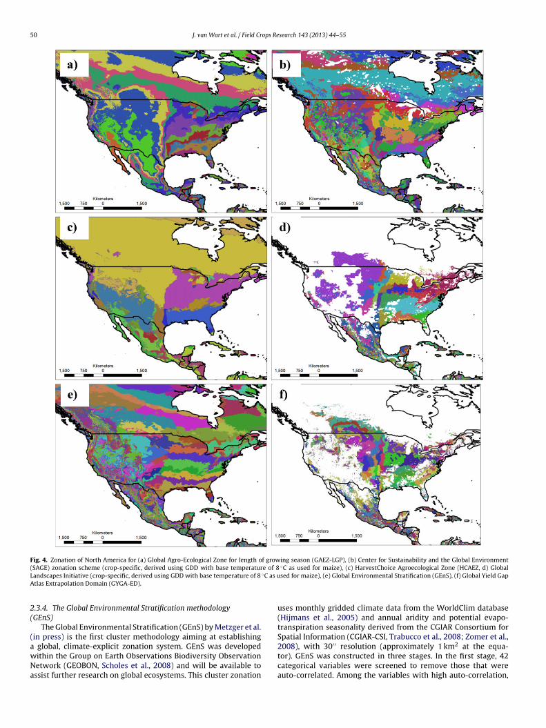

50 J. van Wart et al. / Field Crops Research 143 (2013) 44–55

Fig. 4. Zonation of North America for (a) Global Agro-Ecological Zone for length of growing season (GAEZ-LGP), (b) Center for Sustainability and the Global Environment( e of 8 ◦

L ◦C as uA

2(

(awNa

SAGE) zonation scheme (crop-specific, derived using GDD with base temperaturandscapes Initiative (crop-specific, derived using GDD with base temperature of 8tlas Extrapolation Domain (GYGA-ED).

.3.4. The Global Environmental Stratification methodologyGEnS)

The Global Environmental Stratification (GEnS) by Metzger et al.in press) is the first cluster methodology aiming at establishing

global, climate-explicit zonation system. GEnS was developedithin the Group on Earth Observations Biodiversity Observationetwork (GEOBON, Scholes et al., 2008) and will be available tossist further research on global ecosystems. This cluster zonation

C as used for maize), (c) HarvestChoice Agroecological Zone (HCAEZ, d) Globalsed for maize), (e) Global Environmental Stratification (GEnS), (f) Global Yield Gap

uses monthly gridded climate data from the WorldClim database(Hijmans et al., 2005) and annual aridity and potential evapo-transpiration seasonality derived from the CGIAR Consortium forSpatial Information (CGIAR-CSI, Trabucco et al., 2008; Zomer et al.,

2008), with 30′ ′ resolution (approximately 1 km2 at the equa-tor). GEnS was constructed in three stages. In the first stage, 42categorical variables were screened to remove those that wereauto-correlated. Among the variables with high auto-correlation,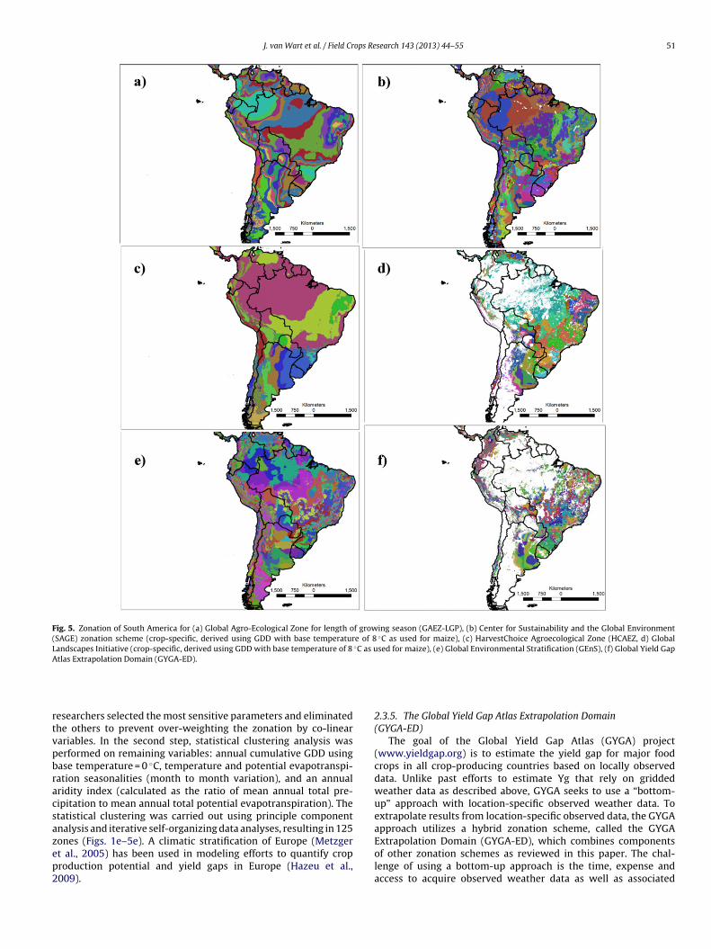

J. van Wart et al. / Field Crops Research 143 (2013) 44–55 51

Fig. 5. Zonation of South America for (a) Global Agro-Ecological Zone for length of growing season (GAEZ-LGP), (b) Center for Sustainability and the Global Environment(SAGE) zonation scheme (crop-specific, derived using GDD with base temperature of 8 ◦C as used for maize), (c) HarvestChoice Agroecological Zone (HCAEZ, d) GlobalLandscapes Initiative (crop-specific, derived using GDD with base temperature of 8 ◦C as used for maize), (e) Global Environmental Stratification (GEnS), (f) Global Yield GapAtlas Extrapolation Domain (GYGA-ED).

rtvpbracsazep2

esearchers selected the most sensitive parameters and eliminatedhe others to prevent over-weighting the zonation by co-linearariables. In the second step, statistical clustering analysis waserformed on remaining variables: annual cumulative GDD usingase temperature = 0 ◦C, temperature and potential evapotranspi-ation seasonalities (month to month variation), and an annualridity index (calculated as the ratio of mean annual total pre-ipitation to mean annual total potential evapotranspiration). Thetatistical clustering was carried out using principle componentnalysis and iterative self-organizing data analyses, resulting in 125

ones (Figs. 1e–5e). A climatic stratification of Europe (Metzgert al., 2005) has been used in modeling efforts to quantify croproduction potential and yield gaps in Europe (Hazeu et al.,009).

2.3.5. The Global Yield Gap Atlas Extrapolation Domain(GYGA-ED)

The goal of the Global Yield Gap Atlas (GYGA) project(www.yieldgap.org) is to estimate the yield gap for major foodcrops in all crop-producing countries based on locally observeddata. Unlike past efforts to estimate Yg that rely on griddedweather data as described above, GYGA seeks to use a “bottom-up” approach with location-specific observed weather data. Toextrapolate results from location-specific observed data, the GYGAapproach utilizes a hybrid zonation scheme, called the GYGA

Extrapolation Domain (GYGA-ED), which combines componentsof other zonation schemes as reviewed in this paper. The chal-lenge of using a bottom-up approach is the time, expense andaccess to acquire observed weather data as well as associated

5 ops Re

laYsnmi

utmtrs1le((fcncnafeoacitm

3z

aottzisu

3

af(ctGtclteftGt

2 J. van Wart et al. / Field Cr

ocation-specific information about crop rotations, soil propertiesnd farm management, which are required for robust estimates ofp and Yw (van Ittersum et al., 2013). Therefore, the GYGA approachtrives for a zonation scheme that balances need to minimize theumber of location-specific sites requiring weather, soils, and cropanagement data with the goal of minimizing climatic heterogene-

ty within the CZs.GYGA-ED is constructed from three categorical variables also

sed by the GEnS: (1) GDD with base temperature of 0 ◦C and (2)emperature seasonality (quantified as the standard deviation of

onthly average temperatures), and (3) an aridity index (annualotal precipitation divided by annual total potential evapotranspi-ation). Grid cell size for the underpinning weather data was theame as for GLI based on the SAGE framework (5′ grid, or roughly00 km2 at the equator). Both GDD and temperature seasona-

ity were calculated using climate data from WorldClim (Hijmanst al., 2005); the aridity index values were taken from CGIAR-CSITrabucco et al., 2008; Zomer et al., 2008). Following Mueller et al.2012), only terrestrial surface covered by at least one of the majorood crops (maize, rice, wheat, sorghum, millet, barley, soybean,assava, potato, yam, sweet potato, banana and plantain, ground-ut, common bean and other pulses, sugarbeets, sugarcane) wasonsidered in this zonation scheme. To avoid inclusion of areas withegligible crop production, only grid cells with sum of the harvestedrea of major food crops > 0.5% of the grid cell area were accountedor, based on HarvestChoice SPAM crop distribution maps (Yout al., 2006, 2009), which update geospatial crop distribution dataf Monfreda et al. (2008). The resulting range in values for GDD andridity index were divided into 10 intervals, each with 10% of gridells with harvested area of the major food crops, and combinedn a grid matrix with 3 ranges of temperature seasonality to give aotal of 300 AEZ classes. Of these, only 265 occur in regions where

ajor food crops are grown.

. Comparison of the agro-climatic and agro-ecologicalonation schemes

Zonation schemes vary widely in defining the size and bound-ries of regions with similar climate (Figs. 1–5). For example, eachf the schemes recognizes the significance of the Sahara desert, buthey differ by as much as 2◦ or 3◦ (roughly 250–350 km) in loca-ion of the southern border in some areas. Differences among theonation schemes are considered in the following sections accord-ng to relevance for assessing performance of crops and croppingystems within a zone, and in the degree of homogeneity of thenderpinning weather variables.

.1. Key variables used within the zonation schemes

All global zonation schemes analyzed in the present study aressociated with temperature and water availability but they dif-er in selection of specific weather variables to delineate zonesTable 1). For example, to account for thermal conditions, GDD isalculated within the SAGE and GLI schemes using crop-specific baseemperatures resulting in a different set of CZs for each crop whileEnS and GYGA-ED use a single, non-crop-specific base tempera-

ure (0 ◦C) to calculate GDD, which gives a single set of CZs for allrops. Creating a different zonation scheme for each crop, however,imits opportunities to analyze Yg for crop rotations and much ofhe world’s cropland produces more than one major food crop. Forxample, crop-specific schemes make it difficult to reconcile per-

ormance of crops within a specific cropping system (e.g. double orriple rice or rice-wheat cropping systems in Asia). In addition toDD, GEnS and GYGA-ED include a measure of temperature varia-

ion during the year based on temperature seasonality.

search 143 (2013) 44–55

Different indexes have been used to quantify the degree of waterlimitation. Water supply in the GLI zonation is calculated as totalannual rainfall. However, this approach does not account for thedegree of water limitation to crop growth, which varies depend-ing on the balance between crop water demand, hereafter calledpotential evapotranspiration, and water supply. In contrast, GAEZ-LGP, HCAEZ, and SAGE try to account for both water supply anddemand using actual and potential evapotranspiration. Specifically,the number of days in which actual evapotranspiration is greaterthan 50% of potential evapotranspiration are used by GAEZ-LGPand HCAEZ to determine when crop growth is possible due to lackof water stress. SAGE considers the ratio of actual evapotranspi-ration to potential evapotranspiration as a soil moisture index.Estimation of actual evapotranspiration is derived from data onsoil texture, bulk density, and depth of root zone (which definesplant-available water-holding capacity), temperature, precipita-tion, and leaf area. The soil components of this estimate are derivedfrom spatially explicit global databases and require a number ofassumptions in order to calculate hydraulic conductivity. Finally,GEnS and GYGA-ED consider an aridity index calculated as theratio of annual total precipitation to annual total potential evapo-transpiration. While not as sophisticated as the GAEZ-LGP or SAGEschemes, this aridity index is derived directly from variables in theweather database and does not require soil data and the associateduncertainties of assumptions used to estimate soil water holdingcapacity.

One of the most influential differences among zonation schemesis whether they define zones over total terrestrial area or only thefraction of that area in which crops are grown. For example, GEnS,GAEZ-LGP, HCAEZ and SAGE all consider total terrestrial area inconstructing their zonation schemes. In contrast, GLI considers onlyharvested area of individual major food crop species to give sep-arate zonation schemes for each crop while GYGA-ED considersone scheme based on harvested area of all major food crops. As aresult the area over which zones are defined is therefore signifi-cantly reduced for those AEZ schemes that only consider harvestedcrop area (Figs. 1–5).

3.2. Climatic variability within the zones

Climate homogeneity for a given zonation scheme was evalu-ated by calculating frequency distributions of the range of grid-cellvalues found within each zone for mean annual temperature,cumulative annual water deficit (precipitation less evapotrans-piration), temperature seasonality, and precipitation seasonality(month to month coefficient of variation in precipitation) based onWorldClim data at 5′ resolution (Hijmans et al., 2005). In addition tocalculating ranges of these variables for each zone in a given zona-tion scheme, ranges of mean annual temperature and cumulativeannual water deficit were calculated only for those cells in whichwheat is grown based on spatial crop distribution of Portmannet al. (2010), in order to minimize bias for those zonation schemesthat are not crop-specific. The geospatial distribution of Portmannet al. (2010) was chosen for use in this analysis over the SPAM orMonfreda et al. (2008) data because these two datasets were usedin the derivation of one or more of the zonation schemes examined.However, it should be noted that climate data used for this analysisare the same as those used in the GEnS, GYGA-ED, and HCAEZ.

3.2.1. Temperature variabilityZone size was largest in GAEZ-LGP and HCAEZ (Table 2). Large

zone area with schemes that consider complete terrestrial cover-

age results in a wide range of within-zone temperature as indicatedby the cumulative frequency distribution of mean annual tem-perature (Fig. 6a). For example, 50% of the GAEZ and HCAEZzones have a range of mean annual temperature > 29 ◦C and 24 ◦C,

J. van Wart et al. / Field Crops Research 143 (2013) 44–55 53

Table 2AEZ scheme coverage of global, China and USA rainfed wheat and maize based on data from Portmann et al. (2010). Values in parenthesis indicate (±SD) of the mean.

AEZ scheme Number of zones Average zone area (Mkm2) Rainfed maize area perzone (Mha)

Number of zones to cover 80% ofrainfed maize harvested area

Global China USA

GAEZ-LGPa 16 20.2 (18.2) 7.5 (7.2) 7 6 4HCAEZb 21 15.3 (28.0) 5.8 (8.2) 6 3 2SAGEc 100 2.7 (4.7) 1.2 (2.1) 28 11 5GLId 100 2.9 (2.0) 1.2 (0.7) 66 37 25GEnSe 125 2.6 (2.5) 1.0 (1.7) 30 13 5GYGA-EDf 265 0.3 (0.3) 0.4 (0.7) 49 21 9

a Global Agro-Ecological Zone Length of Growing Period.b HarvestChoice Agro-ecological Zone.c Center for Sustainability and the Global Environment.d Global Land Initiative.

rsFtawcicnidat

3

toswtwb

3

swsHhetowtREi

3h

ecc

e Global Environmental Stratification.f Global Yield Gap Atlas Extrapolation Domain.

espectively. In contrast, zonation schemes with smaller zoneize have considerably less within-zone temperature variability.or example, the range of mean annual temperature for 50% ofhe GLI and GEnS zones is >4 ◦C. When only cropped terrestrialrea is evaluated (whether for a specific crop or multiple crops),ithin-zone temperature variability decreases substantially. The

lustering methodology of Metzger et al. (in press) also resultedn zones with small ranges in temperature variability despiteonsidering total terrestrial area within zones. Apparently the largeumber of categorical variables considered in the GEnS cluster-

ng scheme results in relatively homogeneous temperature regimeespite complete terrestrial coverage. When only wheat harvestedrea is considered in all zonation schemes, the frequency distribu-ion narrows substantially (Fig. 6b).

.2.2. Water availabilitySimilar to temperature variability within zones, schemes with

he largest zone area (GAEZ-LGP and HCAEZ) have greatest rangef cumulative water deficit (Fig. 6c). Likewise, crop-area zonationchemes, such as GYGA-ED and GLI have greatest homogeneityithin zones. Considering only harvested wheat area within zona-

ion schemes that have complete terrestrial coverage decreases theithin-zone range of water deficit of the zonal schemes somewhat,

ut the range is still relatively large (Fig. 6d).

.2.3. Temperature and precipitation seasonalityThe GYGA-ED, which considers three ranges of temperature

easonality as categorical variables, and the GEnS scheme, forhich temperature seasonality is an explicit input parameter, have

mallest range in temperature seasonality within zones. While theCAEZ, which also accounts for temperature seasonality, has lesseterogeneity for this variable than zonation schemes that do notxplicitly consider it, its large zone size results in a greater rangehan for GYGA-ED. The GAEZ-LGP has the largest within-zone rangef temperature seasonality because its delineation is based more onater availability and many of its zones have relatively large north

o south extension, capturing a wide range of temperature regimes.ange of precipitation seasonality was also smallest in the GYGA-D scheme even though this parameter is not explicitly considered

n its derivation.

.3. Balancing number of zones and within-zone climaticeterogeneity

An appropriate zonation scheme for extrapolating point-basedstimates of yield potential while limiting requirements for dataollection is one which optimizes the trade-off between achievinglimatic homogeneity within zones and minimizing the number of

zones necessary to capture large portions of harvested area of targetcrop. While zonation schemes with few zones and large zone area,such as GAEZ-LGP and HCAEZ, require <10 zones to cover 80% ofglobal rainfed maize harvested area (Table 2), they have large vari-ability in weather variables that influence crop growth and yield(Fig. 6). Among schemes with at least 100 zones and smaller zonesize, those schemes that use the clustering methodology (GEnS)or a three-parameter matrix (GYGA-ED) appear to have the bestbalance between number of zones for 80% coverage of harvestedarea (Table 2) and homogeneity in weather variables within zones(Fig. 6). While the crop-specific GLI zonation scheme has relativelyhomogeneous weather within its zones, it requires the largest num-ber of zones to achieve 80% coverage of rainfed maize area, and itrequires a separate zonation scheme for each crop species. In con-trast, the SAGE scheme requires the smallest number of zones for80% coverage of rainfed maize area but has high degree of variabil-ity in weather variables within its zones despite use of crop-specificbase temperatures used to derive GDD.

4. Discussion

The GAEZ-LGP and HCAEZ schemes are simply too coarse foruse in estimating and extrapolating yield gap analyses becauseclimate heterogeneity within zones is too large. Both SAGE andGLI schemes are crop-specific and use a two-parameter zonationmatrix. Of the two, the GLI approach gives much greater homo-geneity of weather variables within zones, but it requires thelargest number of zones to cover crop area. Both schemes requireseparate zonation schemes for each crop which would make itcumbersome to estimate Yp, Yw, and yield gaps in regions wheremore than one crop was grown in rotation. Both GYGA-ED andGEnS approaches are not crop specific and achieve relatively lowwithin-zone heterogeneity in key weather variables. Whereas GEnSrequires fewer zones to achieve 80% coverage of rainfed maize areaand has slightly less heterogeneity in mean temperature, GYGA-ED has substantially less within-zone heterogeneity in cumulativewater deficit and in seasonality of temperature and precipitation.Both methods appear to be well-suited for up-scaling yield gapanalysis.

Several conclusions follow from this evaluation. Climate zonesused as extrapolation domains for yield gap analysis of current pro-duction should focus on areas where crops are grown to minimizewithin-zone weather variability. While the cluster methodologyalso appears efficient at limiting the number of zones required to

cover crop area and minimizing within-zone heterogeneity, theyare less intuitive than matrix zonation schemes because of thesophisticated mathematics and large number of weather variablesconsidered. However, for matrix-based zonation schemes it has not

54 J. van Wart et al. / Field Crops Research 143 (2013) 44–55

Fig. 6. Frequency distribution of within-zone range of mean annual temperature, annual water deficit (precipitation less evapotranspiration), temperature seasonality andmonth to month coefficient of variation in precipitation based on WorldClim data at 5′ resolution (Hijmans et al., 2005) for 6 climate zonation schemes. All terrestrial areacovered by the zones are considered (panels a, c, e, f); mean annual temperatures and annual water deficit was also calculated considering only where zones overlap wheatharvested area (b and d). The latter evaluation eliminates bias of generic zonation schemes that evaluate all terrestrial area (GAEZ-LGP, GEnS, SAGE, HCAEZ) and all majorc

bb(aadp

ua

rops (GYGA-ED).

een tested how to best determine the range-boundaries, whethery equal distributions (Licker et al., 2010), frequency distributionsGYGA-ED), or another set of criteria such as quantity of harvestedrea within zones (GLI). Beneficial future work would be validationnd comparison of zonation schemes using weather data fromifferent weather stations within a zone or by performing and com-

aring yield gap analysis for several sites within a zone.

All zonation schemes are limited by choice and quality of thenderpinning data used to derive them. This includes availabilitynd distribution of high-quality, location specific weather station

data. Using any zonation scheme to estimate Yp, Yw and yield gapsat larger scales also requires data on soils and management varia-tion within zones (van Ittersum et al., 2013), and quality of thosedata will also affect the accuracy and uncertainty in such large scaleestimates (van Wart et al., 2013).

Acknowledgments

The authors would like to thank the Bill and Malinda Gates Foun-dation whose support of the Global Yield Gap Atlas project made

ops Re

tt

R

A

B

C

E

F

F

F

F

F

F

F

F

F

F

G

G

G

H

H

H

H

J

K

K

L

L

J. van Wart et al. / Field Cr

his research possible. Secondly, we thank Dr. Marc J. Metzger fromhe University of Edinburgh for providing us with the data on GEnS.

eferences

raya, A., Keesstra, S.D., Stroosnijder, L., 2010. A new agro-climatic classification forcrop suitability zoning in northern semi-arid Ethiopia. Agric. Forest Meteorol.150, 1057–1064.

atjes, N.H., 2006. ISRIC-WISE Derived Soil Properties on a 5 by 5 Arc-minutes GlobalGrid. ISRIC–World Soil Information, Wageningen.

aldiz, D.O., Haverkort, A.J., Struik, P.C., 2002. Analysis of a complex crop productionsystem in interdependent agro-ecological zones: a methodological approach forpotatoes in Argentina. Agric. Syst. 73, 297–311.

uropean Environmental Agency (EEA), 2007. Estimating the Environmentally Com-patible Bioenergy Potential from Agriculture. EEA Technical Report 12. EuropeanEnvironmental Agency, Copenhagen.

ood and Agricultural Organization (FAO), 1978. Report on the agro-ecological zonesproject. FAO, Rome.

ischer, G., 2009. World food and agriculture to 2030/50: how do climate change andbioenergy alter the longterm outlook for food, agriculture and resource avail-ability? In: Proceedings of the Expert Meeting on How to Feed the World in2050, FAO Rome, Italy. June 24–26 2009.

ischer, G., Hizsnyik, E., Prieler, S., Shah, M., Van Velthuizen, H., 2009. Biofuels andFood Security. OFID/IIASA, Vienna, p. 40.

ischer, G., Nachtergaele, F.O., Prieler, S., Teixeira, E., Tóth, G., Van Velthuizen, H.,Verelst, L., Wiberg, D., 2012. Global Agro-Ecological Zones – Model Documenta-tion GAEZ v. 3. 0. IIASA/FAO, Laxenburg, Austria/Rome, Italy, p. 179.

ischer, G., Schrattenholzer, L., 2001. Global bioenergy potentials through 2050.Biomass Bioenerg. 20, 151–159.

ischer, G., Shah, M., Tubiello, F.N., Van Velhuizen, H., 2005. Socio-economic andclimate change impacts on agriculture: an integrated assessment, 1990–2080.Phil. Trans. R. Soc. Lond. B 360, 2067–2083.

ischer, G., Shah, M.M., Van Velthuizen, H., Nachtergaele, F.O., 2006. Agroecologi-cal zones assessment. In: Verheye, W.H. (Ed.), Land Use, Land Cover and SoilSciences. EOLSS Publishers, Oxford.

ischer, G., Van Velthuizen, H., Shah, M., Nachtergaele, F.O., 2002. Global agro-ecological assessment for agriculture in the 21st century: methodology andresults. Research Report RR-02-02. International Institute for Applied SystemsAnalysis, Laxenburg, Austria, pp. xxii, 119 pp. and CD-Rom.

oley, J.A., DeFries, R., Asner, G.P., Barford, C., Bonan, G., Carpenter, S.R., Chapin, F.S.,Coe, M.T., Daily, G.C., Gibbs, H.K., Helkowski, J.H., Holloway, T., Howard, E.A.,Kucharik, C.J., Monfreda, C., Patz, J.A., Prentice, I.C., Ramankutty, N., Snyder, P.K.,2005. Global consequences of land use. Science 309, 570–574.

oley, J.A., Ramankutty, N., Brauman, K.A., Cassidy, E.S., Gerber, J.S., Johnston, M.,Mueller, N.D., O’Connell, C., Ray, D.K., West, P.C., Balzer, C., Bennett, E.M., Car-penter, S.R., Hill, J., Monfreda, C., Polasky, S., Rockstrom, J., Sheehan, J., Siebert,S., Tilman, D., Zaks, D.P.M., 2011. Solutions for a cultivated planet. Nature 478,337–342.

allup, J.L., Sachs, J.D., 2000. Agriculture, climate, and technology: why are the trop-ics falling behind? Am. J. Agric. Econ. 82, 731–737.

eerts, S., Raes, D., Garcia, M., Del Castillo, C., Buytaert, W., 2006. Agro-climatic suit-ability mapping for crop production in the Bolivian Altiplano: a case study forquinoa. Agric. Forest Meteorol. 139, 399–412.

odfray, H.C.J., Beddington, J.R., Crute, I.R., Haddad, L., Lawrence, D., Muir, J.F., Pretty,J., Robinson, S., Thomas, S.M., Toulmin, C., 2010. Food security: the challenge offeeding 9 billion people. Science 327, 812–818.

azeu, G., Elbersen, B., Andersen, E., Baruth, B., Van Diepen, C.A., Metzger, M.J.,2009. A biophysical typology for a spatially-explicit agri-environmental mod-eling framework. In: Brouwer, F., Van Ittersum, M.K. (Eds.), Environmental andAgricultural Modelling: Integrated Approaches for Policy Impact Assessment.Springer Academic Publishing, New York/London/Heidelberg/Dordrecht.

azeu, G.W., Metzger, M.J., Mücher, C.A., Perez-Soba, M., Renetzeder, C., Andersen,E., 2011. European environmental stratifications and typologies: an overview.Agric. Ecosyst. Environ. 142, 29–39.

ijmans, R.J., Cameron, S.E., Parra, J.L., Jones, P.G., Jarvis, A., 2005. Very high res-olution interpolated climate surfaces for global land areas. Int. J. Climatol. 25,1965–1978.

oldridge, L.R., 1947. Determination of world plant formations from simple climaticdata. Science 105, 367–368.

ohnston, M., Licker, R., Foley, J., Holloway, T., Mueller, N.D., Barford, C., Kucharik, C.,2011. Closing the gap: global potential for increasing biofuel production throughagricultural intensification. Environ. Res. Lett. 6, 1–11.

öppen, W., 1900. Versuch einer Klassifikation der Klimate, vorzugsweise nach ihrenBeziehungen zur Pflanzenwelt. Geographie Zeitschrift 6, 657–679, 593–611.

ottek, M., Grieser, J., Beck, C., Rudolf, B., Rubel, F., 2006. World Map of the Köppen-Geiger climate classification updated. Meteorologische Zeitschrift 15, 259–263.

icker, R., Johnston, M., Foley, J.A., Barford, C., Kucharik, C.J., Monfreda, C.,

Ramankutty, N., 2010. Mind the gap: how do climate and agriculturalmanagement explain the ‘yield gap’ of croplands around the world? Global Ecol.Biogeogr. 19, 769–782.

obell, D.B., Cassman, K.G., Field, C.B., 2009. Crop yield gaps: their importance, mag-nitudes, and causes. Annu. Rev. Environ. Resour. 34, 179–204.

search 143 (2013) 44–55 55

Metzger, M.J., Bunce, R.G.H., Jongman, R.H.G., Mücher, C.A., Watkins, J.W., 2005. Aclimatic stratification of the environment of Europe. Global Ecol. Biogeogr. 14,549–563.

Metzger, M.J., Bunce, R.G.H., Leemans, R., Viner, D., 2008. Projected environmentalshifts under climate change: European trends and regional impacts. Environ.Conserv. 35, 64–75.

Metzger M.J., Bunce R.G.H, Jongman R.H.G, Sayre R., Trabucco A., Zomer R.A high-resolution bioclimate map of the world: a unifying frameworkfor global biodiversity research and monitoring. Global Ecol. Biogeogr.http://dx.doi.org/10.1111/geb.12022, in press.

Monfreda, C., Ramankutty, N., Foley, J.A., 2008. Farming the planet: 2. geographic dis-tribution of crop areas, yields, physiological types, and net primary productionin the year 2000. Global Biogeochem. Cy. 22, 1–19.

Mueller, N.D., Gerber, J.S., Johnston, M., Ray, D.K., Ramankutty, N., Foley, J.A., 2012.Closing yield gaps: nutrient and water management to boost crop production.Nature 490, 254–257.

New, M., Lister, D., Hulme, M., Makin, I., 2002. A high-resolution data set of surfaceclimate over global land areas. Climate Res. 21, 1–25.

Padbury, G., Waltman, S., Caprio, J., Coen, G., McGinn, S., Mortensen, D., Nielsen,G., Sinclair, R., 2002. Agroecosystems and land resources of the northern GreatPlains. Agron. J. 94, 251–261.

Papadakis, J., 1966. Climates of the World and their Agricultural Potentialities.DAPCO, Rome.

Portmann, F.T., Siebert, S., Doll, P., 2010. MIRCA2000-Global monthly irrigated andrainfed crop areas around the year 2000: a new high-resolution data set foragricultural and hydrological modeling. Global Biogeochem. Cy. 24, GB1011.

Prentice, I.C., Cramer, W., Harrison, S.P., Leemans, R., Monserud, R.A., Solomon, A.M.,1992. Special paper: a global biome model based on plant physiology and dom-inance, soil properties and climate. J. Biogeogr. 19, 117–134.

Ramankutty, N., Foley, J.A., Norman, J., McSweeney, K., 2002. The global distributionof cultivable lands: current patterns and sensitivity to possible climate change.Global Ecol. Biogeogr. 11, 377–392.

Ramirez-Villegas, J., Challinor, A., 2012. Assessing relevant climate data for agricul-tural applications. Agric. Forest Meteorol. 161, 26–45.

Rudolf, B., Beck, C., Grieser, J., Schneider, U., 2005. Global precipitation analysis prod-ucts. Global Precipitation Climatology Centre (GPCC), DWD, Internet publication,pp. 1–8.

Scholes, R.J., Mace, G.M., Turner, W., Geller, G.N., Jürgens, N., Larigauderie, A.,Muchoney, D., Walther, B.A., Mooney, H.A., 2008. Toward a global biodiversityobserving system. Science 321, 1044–1045.

Seppelt, R., 2000. Regionalised optimum control problems for agroecosystem man-agement. Ecol. Model. 131, 121–132.

Sivakumar, M.V.K., Valentin, C., 1997. Agroecological zones and the assessment ofcrop production potential. Phil. Trans. R. Soc. Lond. B 352, 907–916.

TAC/CGIAR (Technical Advisory Committee) Consultative Group on InternationalAgricultural Research, 1992. Review of CGIAR priorities and strategies. Part I.Washington DC: CGIAR.

Tilman, D., Cassman, K.G., Matson, P.A., Naylor, R., Polasky, S., 2002. Agriculturalsustainability and intensive production practices. Nature 418, 671–677.

Tou, J.T., González, R.C., 1974. Pattern recognition principles. Addison-Wesley Pub-lishing Co. Reading, MA.

Trabucco, A., Zomer, R.J., Bossio, D.A., van Straaten, O., Verchot, L.V., 2008. Cli-mate change mitigation through afforestation/reforestation: a global analysisof hydrologic impacts with four case studies. Agric. Ecosyst. Environ. 126,81–97.

van Ittersum, M.K., Cassman, K.G., Grassini, P., Wolf, J., Tittonell, P., Hochman, Z.,2013. Yield gap analysis with local to global relevance–a review. Field Crop Res.143, 4–17.

van Wart, J., Kersebaum, K.C., Peng, S., Milner, M., Cassman, K.G., 2013. A protocolfor estimating crop yield potential at regional to national scales. Field Crops Res.143, 34–43.

Williams, C.L., Liebman, M., Edwards, J.W., James, D.E., Singer, J.W., Arritt, R., Herz-mann, D., 2008. Patterns of regional yield stability in association with regionalenvironmental characteristics. Crop Sci. 48, 1545–1559.

Wood, S., Pardey, P.G., 1998. Agroecological aspects of evaluating agricultural R andD. Agric. Syst. 57, 13–41.

Wood, S., Sebastian, K.L., Scherr, S., 2000. Pilot analysis of global ecosystems: agroe-cosystems. In: Joint Study by the International Food Policy Research Instituteand the World Resources Institute. World Resources Institute, Washington, DC.

Wood, S., Sebastian, K.L., You, L., 2010. Spatial perspectives. In: Pardey, P.G., Wood,S., Hertfor, R. (Eds.), Research Futures: Projecting Agricultural R&D Potentials forLatin America and the Caribbean. International Food Policy Research Institute,Washington, DC.

You, L., Wood, S., Wood-Sichra, U., 2006. Generating global crop maps: from cen-sus to grid. In: Selected paper, IAAE (International Association of AgriculturalEconomists) Annual Conference, Gold Coast, Australia.

You, L., Crespo, S., Guo, Z., Koo, J., Sebastian, K., Tenorio, M.T., Wood, S., Wood-Sichra, U. 2009. Spatial Production Allocation Model (SPAM) 2000 Version 3

Release 6.

Zomer, R.J., Trabucco, A., Bossio, D.A., Verchot, L.V., 2008. Climate change mit-igation: a spatial analysis of global land suitability for clean developmentmechanism afforestation and reforestation. Agric. Ecosyst. Environ. 126,67–80.

Assessment of rice self-sufficiency in 2025 in eight

African countries P.A.J. van Oort, K. Saito, A. Tanaka, E. Amovin-Assagba, L.G.J. Van Bussel, J. van Wart, H. de Groot, M.K. van Ittersum, K.G. Cassman,

M.S.C. Wopereis 2015, Global Food Security, Volume 5: 39-49

http://www.sciencedirect.com/science/article/pii/S2211912415000036

Assessment of rice self-sufficiency in 2025 in eight African countries

P.A.J. van Oort a,b,n, K. Saito a, A. Tanaka a, E. Amovin-Assagba a, L.G.J. Van Bussel c,J. van Wart d, H. de Groot e, M.K. van Ittersum c, K.G. Cassman d, M.C.S. Wopereis a

a Africa Rice Center, 01 BP 2031, Cotonou, Beninb Centre for Crop Systems Analysis, Wageningen University, PO Box 430, NL-6700 AK Wageningen, Netherlandsc Plant Production Systems, Wageningen University, PO Box 430, NL-6700 AK Wageningen, Netherlandsd Department of Agronomy and Horticulture, University of Nebraska–Lincoln, 202 Keim Hall, Lincoln, NE 68583-0915, USAe WUR – Alterra – Earth Observation and Environmental Informatics, PO Box 47, 6700 AA Wageningen, Netherlands

a r t i c l e i n f o

Article history:Received 25 July 2014Received in revised form9 January 2015Accepted 13 January 2015

Keywords:Food securityPopulationRiceYield gapYield potentialAfrica

a b s t r a c t

Most African countries are far from self-sufficient in meeting their rice consumption; in eight countriesthe production: consumption ratio, ranged from 0.16 to 1.18 in 2012. We show that for the year 2025,with population growth, diet change and yield increase on existing land (intensification), countriescannot become fully self-sufficient in rice. This implies that for the future, a mixture of area expansionand imports will be needed on top of yield gap closure. Further research is needed for identification ofmost suitable new land for rice area expansion and areas that should be protected.& 2015 The Authors. Published by Elsevier B.V. This is an open access article under the CC BY license

(http://creativecommons.org/licenses/by/4.0/).

1. Introduction

Faced with a growing population and increasing per capita riceconsumption, countries and their policy makers have threeoptions to meet future demand for rice: increase imports, increaserice area and increase production per unit area. Often, growingneeds are met through a combination of these three options. Butin some cases one or more of these solutions are not possible, oronly to a limited extent. Such is the case when biophysical limits toyield increase have been reached, or where all of the suitable landis already being used for agriculture or cultivation of specific crops.It is therefore relevant to quantify the biophysical opportunitiesand limits. Many African politicians have formulated ambitiousplans for increasing production (Seck et al., 2012, 2013, www.riceforafrica.org). It is therefore timely to investigate the quanti-tative relationship between self-sufficiency or import levels on theone hand and yield gap closure and area expansion on the otherhand. We do not make (political or societal) statements on whichmixture of imports, area expansion and yield increase is mostdesirable or most realistic politically. Rather, we compute thewindow of opportunities between these key variables. Rather we

aim to quantify trade-offs between imports and area expansionfor rice cultivation. These trade-offs depend on uncertain futuretrends in per capita consumption and yield increase. We thereforepresent different scenarios to quantify the range of possibleoutcomes. Such an analysis is also relevant in the context ofstudies on “intensification” (raising yields on existing fieldsthrough yield gap closure). Most recent studies consider intensi-fication the most desirable option, due to concerns about landavailability and quality, and the need to protect natural ecosystems(Tilman et al., 2002; Cassman et al., 2003; Koning and vanIttersum, 2009; Foley et al., 2011; Pretty et al., 2011; Ramankuttyand Rhemtulla, 2012; Garnett et al., 2013; Hall and Richards, 2013).

In Africa, with its rapid population growth, agricultural areahas been expanding and is likely to continue. This expansion hasoccurred because yield increase on existing land has been too slowto keep up with growing consumption in most African countries(Pretty et al., 2011). The future required agricultural area can beestimated based on extrapolation of current trends in yield andconsumption (e.g. Balmford et al., 2005). Such approaches havebeen criticized (e.g., van Ittersum et al., 2013) because suchextrapolations may lead to yield projections above the biophysicalupper limits imposed by solar radiation, temperature, and watersupply (which is impossible). Quantification of the biophysicalupper limits to yield increase through the use of crop growthmodels may help more realistic quantification of the extent towhich self-sufficiency can be achieved through intensification.

Contents lists available at ScienceDirect

journal homepage: www.elsevier.com/locate/gfs

Global Food Security

http://dx.doi.org/10.1016/j.gfs.2015.01.0022211-9124/& 2015 The Authors. Published by Elsevier B.V. This is an open access article under the CC BY license (http://creativecommons.org/licenses/by/4.0/).

n Corresponding author at: Center for Crop Systems Analysis, WageningenUniversity, PO Box 430, NL-6700 AK Wageningen, Netherlands. Tel.: þ31 0 317481357; fax: þ31 0 317 485572.

E-mail address: pepijn.vanoort@wur.nl (P.A.J. van Oort).

Global Food Security 5 (2015) 39–49

Since 2000, both rice harvested area and yield have beenincreasing in Sub-Saharan Africa (SSA) (Fig. 1a and b). However,the ratio between production and consumption (P/C ratio), whichis an indicator for self-sufficiency, has been far below one for aconsiderable time (Fig. 1c), indicating that most countries in SSAare still far from being self-sufficient in rice. Meanwhile, thepopulation (UN, 2014, Fig. 1d) and per-capita consumption areexpected to continue to increase. If growth in yields cannot keeptrack of growth in consumption then either more area, moreimports, or a combination of these two will be needed.

With a growing population and changing diets policy makershave basically three options to meet future consumption needs:(1) increase yields, (2) increase imports and (3) area expansion. Aconceptual model of the decision-making space is shown in Fig. 2.For a given population and at given yield levels and diet, any linearcombination of area and imports can fulfill the population's needs.If population grows or if per capita consumption grows, theneither more imports or more area will be needed. If yields increasethen less imports or less area will be needed. The area in betweenthe dashed lines shows the biophysical boundaries within whichchoices are made. These lines are dashed because they reflectuncertainty about future trends in population growth, diet changeand yield increase. There is a clear trade-off between the politicalchoice to reduce imports (which may require further area expan-sion) and the political choice to reduce area expansion (andremain dependent on international markets for imports).The biophysical boundaries within which this economic, societaland political decision making will take place are still not wellquantified.

The objective of this paper is to quantify the trade-offs betweenarea expansion and import dependency at different levels of yieldincrease and diet change. We present scenarios for the year 2025for eight African countries. We choose this relatively near timehorizon since it is meaningful for most African policy makers. The

objective of this study is to assess self-sufficiency scenarios with alonger time horizon suffer from increased uncertainty of populationgrowth scenarios (Hopfenberg and Pimentel, 2001; Alexandratos,2005; Dyer, 2013), increased uncertainty in estimates of availablearea (Andriesse, 1986; Windmeijer and Andriesse, 1993; Young,1999; Ramankutty et al., 2002; You et al., 2011; Byerlee et al., 2014),and uncertainty about climate change impacts (which for rice inAfrica have not yet been clearly quantified). The choice of seven SSAcountries was driven by the Global Yield Gap Atlas project (GYGA,www.yieldgap.org) on which the results presented here are based.Egypt was included as a benchmark for an African country whereyield gaps are expected to be small.

Fig. 1. Trends in harvested area (a), yield (b), production/consumption (c) and population (d). (Based on USDA (2014) and UN (2014)).

Fig. 2. Conceptual model of trade-offs between area and imports, with effects ofyield increase, population growth and growth in per capita consumption.

P.A.J. van Oort et al. / Global Food Security 5 (2015) 39–4940

2. Methods

We first describe a framework used for calculating rice self-sufficiency at the national level in the eight countries (BurkinaFaso, Egypt, Ghana, Mali, Nigeria, Tanzania, Uganda, and Zambia).We describe the method of selection of sites at subnational level,an approach used for calculations of actual and potential yields ineach site, and input data used for the calculations. The actual andpotential yields estimated at the subnational level were aggre-gated to the national level. We then provide the calculationmethods for rice harvested area and consumption at national level.

2.1. Rice self-sufficiency

Self-sufficiency calculations can be reduced to a simple equa-tion of production and consumption. We use the production–consumption ratio (P/C) as an indicator of self-sufficiency, where acountry is self-sufficient at P/C¼1. Production depends on har-vested area and yield, consumption depends on population andper-capita consumption. For a given consumption, we can calcu-late what harvested area and yield levels are needed to makeproduction meet consumption. Total rice production for a countrywas calculated as

Punmilled ¼HArf � Yrf þHAir � Yir ð1Þ

where Punmilled is production (thousands of tonnes) of unmilledrice; HArf and HAir are harvested areas of rainfed and irrigated rice(thousands of hectares); Yrf is the yield of rainfed rice (t/haunmilled rice, at 14% moisture content); and Yir is the same forirrigated rice. Three yield levels (Ya, Yw, and Yp) are considered:

Ya current average yield of unmilled rice, with Yarf and Yairfor rainfed and irrigated systems, respectively.

Yp yield potential, determined by temperature and solarradiation during the crop production period, assumingno limitations on water or nutrient supply and no loss ofyield to toxicities, insects or other herbivores, diseases, orweeds; Yp was used as the benchmark for irrigated rice.

Yw water-limited yield potential, governed by temperature,solar radiation, rainfall, soil properties, and landscapeposition that govern root-zone water-holding capacityand runoff, assuming no limitations on crop yield due tonutrient deficiencies, toxicities, insects or other herbi-vores, diseases, or weeds; Ywwas used as the benchmarkfor rainfed rice.

From these we calculated absolute yield gaps (Yp�Yair forirrigated rice and Yw�Yarf for rainfed rice) and relative yieldsYair/Yp and Yarf/Yw. The distinction between irrigated rice andrainfed rice is important because actual yields and yield potentialare much higher in irrigated rice. Within rainfed rice a distinctionwas made between rainfed upland and rainfed lowland. Rainfedupland soils are generally located higher in the landscape, havestronger drainage, and deeper groundwater levels in comparisonwith lowland. Soil fertility is often lower in upland soils comparedto the lowlands. We calculated Yw separately for upland andlowland conditions and then aggregated to rainfed Yw valuesusing the relative areas of upland and lowland rice area at eachsite (site selection and aggregation to national level is described inSection 2.2).

Total rice consumption is normally expressed in kilograms ofmilled rice. In rice milling, the husk and bran layers are removed toreveal the edible, white rice kernel. In this process, dependingon the quality of the unmilled rice and the mills, 30–40% of the

weight is removed. We calculated milled production as

Pmilled ¼ 0:65� Punmilled ð2ÞDomestic consumption or consumption depends on population

(expressed in millions) and per-capita consumption (kg person�1

year�1)

Cmilled ¼ Population� Per capita consumption ð3Þwhere Dmilled is domestic consumption for milled rice (thousandsof tonnes). In the rice self-sufficiency scenarios we calculated whatis needed to make production match consumption. We added toeach production term a possible change in average yield andproduction area (Δ)

Cmilled ¼ 0:65� ½ðHArf þΔHArf Þ � ðYarf þΔYrf ÞþðHAirþΔHAirÞ � ðYairþΔYirÞ� ð4Þ

Once three of the Δs are fixed, the fourth can be calculated, forexample ΔHAir becomes

ΔHAir ¼ ½Cmilled=0:65–ðHArf þΔHArf Þ�ðYarf þΔYrf Þ�=ðYairþΔYirÞ–HAir ð5Þ

Laborte et al. (2012), based on Koning and van Ittersum (2009),identify five ways to close the production gap: (1) expansion ofland under cultivation, (2) intensification on existing farmland bygrowing two or three crops a year, (3) narrowing the yield gap infarmers' fields through introducing new technologies, (4) raisingthe yield ceiling by introducing higher-yielding cultivars, and(5) reducing postharvest losses. We consider options 1–3 here,where option 1 is physical area expansion and options 2 and 3 areintensification options.

Harvested area can be larger than physical area because insome areas two rice crops can be grown in the same field in oneyear. A national weighted average rice cropping intensity CIir wascalculated weighted by areas under single and double rice crop-ping (see Section 2.2). For example, if CIir¼1.6 then 60% of thefarmers' fields will have two rice crops per year and 40% one ricecrop per year. For a given value of CIir we can convert harvestedarea expansion (ΔHAir) into physical area expansion (ΔAir)

ΔAir ¼ΔHAir=CIir ð6ÞFor rainfed systems a similar equation (ΔArf¼ΔHArf/CIrf) can be

applied. However, our data indicated no double rice cropping inany of the rainfed rice areas, so a value of CIrf¼1 was used for allestimations of rainfed rice production. In the irrigated rice areas,CIir ranged from 1 to 2. There is anecdotal evidence of farmersgrowing three rice crops per year, but considering the tightpressure that this puts on logistics and need to grow other crops,we do not consider triple rice crops a realistic option on a largescale. In Egypt, minimum temperatures are often below 15 1C fromNovember to April (6 months). High levels of cold sterility can beexpected at those temperatures, so intensification by shifting fromone to two rice crops per year on the same land is not possible.Therefore for Egypt we did not allow CIir to increase. We assumedthat intensification on existing farmland would only be possible onirrigated land in the tropical zone in African countries, and to amaximum of two crops per year (except Egypt for which CIir¼1).Thus the maximum expansion of harvested area rice on existingirrigated rice land can be calculated as:

MaxfΔHAirg ¼ Air � 2:0–CIirð Þ ð7ÞLikewise we constrained maximum yield increases ΔYrf and

ΔYir within biophysically and economically realistic bounds

MaxfΔYrf g ¼ ð0:8� Ywrf Þ–Yarf ð8Þ

MaxfΔYirg ¼ ð0:8� YpirÞ–Yair ð9Þ

P.A.J. van Oort et al. / Global Food Security 5 (2015) 39–49 41

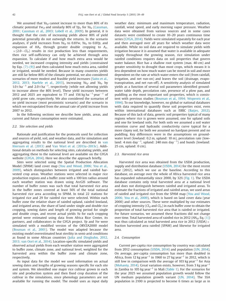
We assumed that Yarf cannot increase to more than 80% of itsclimatic potential Ywrf and similarly 80% of Ypir for Yair (Cassman,2001; Cassman et al., 2003; Lobell et al., 2009). In general, it isthought that the costs of increasing yields above 80% of yieldpotential generally do not outweigh the returns. In the scenarioanalyses, if yield increases from Yarf to 0.8Yw, Yair to 0.8Yp, andexpansion of HAir through greater double cropping to Air-

� (2.0�CIir) results in rice production less than requirements,then rice self-sufficiency can only be achieved through areaexpansion. To calculate if and how much extra area would beneeded, we increased cropping intensity and yields (constrainedby Eqs. (7)–(9)) and then calculated how much extra area, rainfedor irrigated, would be needed. Because in many countries yieldsare still far below 80% of the climatic potential, we also consideredscenarios of more modest and feasible yield increases (Saito et al.,2012, 2013; Haefele et al., 2013), increasing Yarf and Yair by1.0 t ha�1 and 2.0 t ha�1, respectively (while not allowing yieldsto increase above the 80% level). These yield increases between2012 and 2025 are equivalent to 77 and 156 kg ha�1 year�1 ofyield grow rate, respectively. We also considered the scenarios ofno yield increase (most pessimistic scenario) and the scenario inwhich we extrapolated from the annual rate of yield increase from2007 to 2012.

In the following sections we describe how yields, areas, andcurrent and future consumption were estimated.

2.2. Site selection and yields

Rationale and justification for the protocols used for collectionand sources of yield, soil, and weather data, and for simulation andaggregating results to the national level are described in vanIttersum et al. (2013) and Van Wart et al. (2013a–2013c). Addi-tional details on methods for selecting sites, calculating yields, andaggregating these to the national level are available on the GYGAwebsite (GYGA, 2014). Here we describe the approach briefly.

Sites were selected using the Spatial Production AllocationModel (SPAM) land cover map (You and Wood, 2006; You et al.,2009), which distinguishes between irrigated and rainfed har-vested crop areas. Weather stations were selected in major riceproduction regions and a buffer zone with a 100 km radius aroundeach weather station was drawn using ArcGIS software. Thenumber of buffer zones was such that total harvested rice areain the buffer zones covered at least 50% of the total nationalharvested rice area according to SPAM. In total 22 stations forirrigated rice and 29 for rainfed rice were selected. Within eachbuffer zone the relative share of rainfed upland, rainfed lowland,and irrigated areas, the share of land under single and double ricecropping, sowing dates and length of growing period for singleand double crops, and recent actual yields Ya for each croppingperiod were estimated using data from Africa Rice Center, itspartners, and collaborators in the GYGA project. Yp and Yw weresimulated with a modified version of the ORYZA2000 model(Bouman et al., 2001). The model was adapted because theexisting model overestimated heat sterility in semi-arid conditionsas found in some African countries (Julia and Dingkuhn, 2012,2013; van Oort et al., 2014). Location-specific simulated yields andobserved actual yields from each weather station were aggregatedto buffer zone, climate zone, and national level, weighted for theharvested area within the buffer zone and climate zone,respectively.

As input data for the model we used information on actualsowing dates and lengths of growing seasons specific for each siteand system. We identified one major rice cultivar grown in eachsite and production system and then fixed crop duration of thecultivar in the simulations, since phenology parameters are notavailable for running the model. The model uses as input daily

weather data: minimum and maximum temperature, radiation,rainfall, wind speed, and early morning vapor pressure. Weatherdata were obtained from various sources and in some casesdatasets were combined to create 10–20 years continuous timeseries (GYGA, 2014). Yields were simulated separately for each yearand then averaged over all years for which weather data wereavailable. While no soil data are required to simulate yields withirrigation because it is assumed that water is available in adequatesupply throughout the growing season, rice simulation underrainfed conditions requires data on soil properties that governwater balance. Rice has a shallow root system (max. 40 cm) andgreater sensitivity to drought than most crops, which means it isless dependent on how much water can be stored in soil and moredependent on the rate at which water enters the soil (from rainfall,irrigation, and net run-on) and leaves the soil (drainage, evapo-transpiration, and net run-off). A sensitivity analysis of simulatedyields as a function of several soil parameters identified ground-water table depth, percolation rate, presence of a plow pan, andpuddling as the most important soil properties, which is consis-tent with previous studies (Bouman et al., 1994; Wopereis et al.,1994). To our knowledge, however, no global or national databaseswith data required to quantify these soil properties exist, evenwithin international databases such as ISRIC (Batjes, 2012).Because of this lack of data, generic soil properties typical of manyregions where rice is grown were assumed, one for upland soilsand one for lowland soils. For both soils we assumed a soil waterretention curve and hydraulic conductivity curve typical for amore clayey soil, for both we assumed no hardpan present and nopuddling. Key differences were in the assumptions on ground-water level (lowland: 0.2 m, upland: 10 m), percolation rate (low-land: 4 mm day�1, upland: 240 mm day�1) and bunds (lowland:25 cm, upland: 0 cm).

2.3. Harvested rice area

Harvested rice area was obtained from the USDA production,supply and distribution database (USDA, 2014) for the most recentyear (2012), which we use as the baseline. According to thisdatabase, on average over the whole of Africa harvested rice areahas expanded substantially since 2000, by 32% (Fig. 1). The USDAdatabase contains only total harvested area at a national leveland does not distinguish between rainfed and irrigated areas. Toestimate the fractions of irrigated and rainfed areas, we used areasof rainfed and irrigated rice from the SPAM map (You and Wood,2006; You et al., 2009), which is based on land cover data (year2000) and other sources. These were multiplied by our estimatesof cropping intensity (CIrf and CIir) in each buffer zone to obtain theproportion of total harvested rice area that is rainfed or irrigated.For future scenarios, we assumed these fractions did not changeover time. Total harvested area of rainfed rice in 2012 (HArf, Eq. (1))was thus calculated as total harvested area rice in 2012 (USDA)�fraction harvested area rainfed (SPAM) and likewise for irrigatedarea.

2.4. Consumption

Current per-capita rice consumption by country was calculatedfrom 2012 consumption (USDA, 2014) and population (UN, 2014).On average, per-capita consumption has more than doubled inAfrica, from 12 kg year–1 in 1960 to 27 kg year–1 in 2012, which isstill low in comparison with the average of 103 kg year–1 for Asia(Mohanty, 2014). Great variation exists, however, from 3 kg year–1

in Zambia to 105 kg year–1 in Mali (Table 1). For the scenarios forthe year 2025 we assumed population growth would follow theUN medium population growth variant (UN, 2014). The SSApopulation in 2100 is projected to become 6 times as large as in

P.A.J. van Oort et al. / Global Food Security 5 (2015) 39–4942

2000 (Fig. 1d). For 2025 relative to 2012, population for SSA isexpected to increase by a factor 1.39. For the countries included inthis study, population is expected to increase by between factorsof 1.2 (Egypt) and 1.52 (Zambia).

To calculate future rice consumption, we multiplied populationby per-capita consumption. In one set of scenarios we assumed nochange in diet, in the other set of scenarios we extrapolated per-capita consumption from the trend in the period 2000–2012. Inthis period per-capita consumption increased by 7–9% per year inBurkina Faso, Mali, and Zambia, 4–5% in Ghana and Nigeria, and 0%in Egypt, Tanzania, and Uganda.

2.5. Scenarios

The future for yield increase is uncertain, as is the future fordiet change. Both are in part dependent on autonomous develop-ment and to in part they may be influenced by policy makers. Forexample, increased investments in subsidies on inputs (seeds,fertilizer, pesticides, etc.) can lead to increased yields. To copewith uncertainties in future yield and diet change we included arange of scenarios for yield increase and a two scenarios for dietchange. In the most pessimistic scenario, yields would stagnate. Inthe middle scenarios yields would continue to increase followingthe trend since 2007 (Table 2). These trends are of a similar orderof magnitude as the scenarios of 1 or 2 t ha�1 of yield increasefrom 2012 to 2025, which corresponds with average trends of 78or 156 kg ha–1 year–1. These two yield trends are lower and higherthan the recent yield trend in SSA of about 100 kg ha–1 year–1 since2007 (Seck et al., 2013). In SSA, even with a 1 or 2 t ha�1 yieldincrease, the yields would still be far below the biophysicalmaximum (Fig. 3). At the biophysical and economic extreme endof the spectrum yields could be increased to 80% of potential (Ywor Yp).

3. Results

3.1. Current situation

On average over all simulated sites, all cropping patterns (wetor dry season cropping), and all production systems, actual yieldsare only 38% of their potential and within a range of 10–70% exceptfor the Nile Delta in Egypt, where actual yield is about 80% of Yp(Fig. 3). In SSA, actual yields in rainfed systems range from 1 to3 t ha�1, while actual yields in irrigated systems range from 2to 6 t ha�1. In irrigated systems, actual and potential yields are

higher in the dry season than in the wet season. Relative yields(Ya/Yw for rainfed and Ya/Yp for irrigated) are lowest in the rainfedupland and lowland (average 0.27), followed by irrigated lowlandin the wet season (0.4), and irrigated lowland in the dry season(0.55).

The production–consumption ratios (P/C) in 2012 ranged from0.16 to 1.18 in the eight African countries (Table 1). Egypt is morethan self-sufficient, and Mali, Tanzania, and Uganda are close tobeing self-sufficient (Table 1). In contrast, Burkina Faso, Ghana,Nigeria, and Zambia are far from being self-sufficient. Table 2 andFig. 1 show high rates of yield increase since 2007. These rates ofyield increase are still far lower than in the scenario where yieldsin 2025 are at 80% of Yw or Yp (Table 2). To achieve yields of 80% ofYw or Yp by 2025 would require a significant acceleration relativeto the current yield trend (Table 2). It is questionable whether thisis realistic to expect.

3.2. Scenarios 2025

The trade-off between area used for rice and imports, based onTables 1–5, is shown in Fig. 4. The black dot in the middle is thesituation in 2012. We describe Burkina Faso as an example. The leftpane shows that at current yield trends and unchanged diet, importsor area would need to increase a bit (blue line). In case of no area

Table 1Rice self-sufficiency for current consumption under different production scenarios.

Consumption (Mt) in 2012 Production (Mt) in 2012 Imports (Mt) in 2012 Production/consumption (P/C) Consumptiona

(kg person�1 year�1)

2012 2025

Burkina Faso 0.640.32

0.32 0.49 25 35

Ghana 1.46 0.24 1.22 0.16 37 45Mali 2.39 2.14 0.25 0.89 105 156Nigeria 9.13 4.81 4.32 0.53 35 44Tanzania 1.69 1.41 0.28 0.83 23 24Uganda 0.27 0.27 0 0.99 5 5Zambia 0.06 0.04 0.02 0.57 3 5Egypt 6.00 7.10 �1.1 1.18 48 51Total 21.65 16.32 5.33 0.75Tot. excl. Egypt 15.65 9.22 6.43 0.59

Sources: bUSDA (2014).a USDA (2014) and UN (2014).

Table 2Recent yield trend and yield trend needed to achieve 80% of the potential.

Yield trend 2007–2012 (kg ha�1 year�1)a Yield trend neededto get from Ya to80% of Yp or Ywfrom 2012 to 2025(kg ha�1 year�1)b

Rainfed Irrigated

Burkina Faso 88 254 277Ghana 169 431 305Mali 127 198 305Nigeria 117 295 382Tanzania �108 246 306Ugandac 29 211Zambiac 196 529Egyptc �229 �18

Sources:a USDA (2014).b GYGA (2014).c For Uganda and Zambia there are currently no large areas used for irrigated

rice production. There is no rainfed agriculture in Egypt.

P.A.J. van Oort et al. / Global Food Security 5 (2015) 39–49 43

expansion, imports would increase from 0.32 Mt/year (Table 1) to0.42 Mt/year (Table 3) or in case of striving for full self-sufficiency,area would need to increase. Table 5 shows that either rainfed areawould need to increase from 87 to 248 thousand hectares or irrigatedarea increase from 33 to 87 thousand hectares. For Burkina Faso withthe current yield trend and increased per capita consumption (from25 to 35 kg/person/year, Table 1), large increases in area and/orimports would be needed (red line). Thus diet changes can have alarge impact on projections of future import and area needs (red vs.blue line). In 2012 the Burkina Faso P/C ratio was 0.49, indicating ahigh dependence on imports (Table 1, Fig. 4 right pane). If for politicalor economic reasons a higher P/C ratio is desired then the associated

extra area can be looked up in Fig. 4 in the right pane. For example aP/C ratio of 0.8 can be achieved by increasing irrigated area from0.033 Mha to around 0.065 Mha (blue line) or 0.100 Mha (red line).The green and purple graphs in Fig. 4 show the trade-off betweenarea and imports or P/C ratios in case yields are increased to 80% ofthe biophysical potential.

The right panes in Fig. 4 show how self-sufficiency in relativeterms would change under different scenarios of yield increaseand change in area, for all the 8 countries. With current rates ofyield increase, none of the countries can become fully self-sufficient in rice without area expansion (Fig. 4, red and bluelines). With maximally accelerated rates of yield increase over2012–2025, five countries could become net exporters (Fig. 4,green and purple lines). For Burkina Faso, Ghana, Nigeria andZambia, which are far from being self-sufficient in rice in 2012,self-sufficiency ratios would still remain below far below one atcurrent yield trends. For Mali, Tanzania and Uganda, close to beingself-sufficient in rice in 2012, the scenarios differ between coun-tries. For Mali, self-sufficiency would stay the same in case of nodiet change; self-sufficiency would strongly decrease in case ofdiet change. For Tanzania and Uganda projected changes in dietare small. Under both scenarios, self-sufficiency would dramati-cally decrease. But with rates of yield increase of 1 t/ha, these twocountries could still remain self-sufficient without additional areaexpansion (Table 4). Egypt was a net exporter in 2012 (Table 1:P/C¼1.18). With projected population increase and no change inrice area, the country would change into a small net importer(Table 4: P/C¼0.92–0.99).

Although full self-sufficiency may not be economically optimal,or politically realistic, the analysis of the extra required area in theextreme case of full self-sufficiency provides an indication of howmuch extra area would be needed at most. Rainfed area wouldneed to become on average over the eight countries 2.5 times aslarge (Table 5: 7562/2990), ranging between 1.4 in Uganda andZambia to 4.3 in Burkina Faso and Ghana. If expansion were tocome from irrigated area only, irrigated area would on averageneed to expand by a factor 2.5 (3.4 excluding Egypt), rangingbetween 1.1 in Egypt to 19.2 in Ghana. The required relativeexpansion in Ghana from irrigated land is large because there isrelatively little irrigated land, so irrigated land contributes very

Fig. 3. Simulated and actual yields for all sites in Africa simulated in the GlobalYield Gap Atlas (GYGA) project. Lines shown are the 1:1 line, relative yields at 10%and 70% of potential yields, and the regression line through all data points.

Table 3Imports (Mt) for scenarios 2025 with no area expansion.

Imports (Mt rice at 14% moisture)

Current diet Diet extrapolated based on trend 2000–2012

No yieldincrease

Y trend'07–'12

Yieldþ1 t ha�1

Yieldþ2 t ha�1

Yield to 80% ofYp or Yw

80%þdoublecrop

No yieldincrease

Y trend'07–'12

Yieldþ1 t ha�1

Yieldþ2 t ha�1

Yield to 80% ofYp or Yw

80%þdoublecrop

BurkinaFaso

0.60 0.42 0.45 0.29 0.07 0.07 0.95 0.77 0.79 0.64 0.42 0.42

Ghana 1.64 1.26 1.47 1.30 0.72 0.68 2.04 1.66 1.87 1.70 1.11 1.08Mali 1.46 0.38 0.81 0.16 �0.79 �2.85 3.20 2.13 2.55 1.90 0.96 �1.11Nigeria 8.16 4.73 3.66 3.66 �1.36 �7.14 11.59 8.15 7.09 7.09 2.07 �3.71Tanzania 1.04 1.04 0.09 �0.86 �2.05 �2.20 1.17 1.17 0.22 �0.73 �1.93 �2.07Uganda 0.14 0.09 0.00 �0.14 �0.24 �0.24 0.15 0.10 0.01 �0.13 �0.23 �0.23Zambia 0.06 �0.02 0.03 0.00 �0.15 �0.15 0.12 0.05 0.09 0.06 �0.08 �0.08Egypt 0.10 0.10 0.10 0.10 0.28 0.28 0.47 0.47 0.47 0.47 0.64 0.64Total 13.20 8.02 6.61 4.52 �3.52 �11.54 19.69 14.50 13.09 11.00 2.96 �5.06Total excl.Egypt

13.10 7.91 6.51 4.41 �3.80 �11.82 19.22 14.03 12.63 10.53 2.32 �5.70

No yield increase¼yields fixed to levels as reported in the GYGA project; Y trend '07–'12¼yields from GYGA-projected increase following annual national trend from 2007 to2012 derived from USDA (2014); Yield þ1 t ha�1¼all yields from GYGA increased by 1 t ha�1; Yield þ2 t ha�1¼all yields from GYGA increased by 2 t ha�1; Yield to80%¼yields increased to 80% of the biophysical potential (Yw or Yp); 80%þdouble crop¼yields increased to 80% of the biophysical potential and cropping intensity onirrigated land increased from current CIir to CIir¼2 (except for Egypt: CIir¼1).

P.A.J. van Oort et al. / Global Food Security 5 (2015) 39–4944

little to total production. For Burkina Faso, Ghana, Mali, Nigeria,and Tanzania, rice physical area in 2025 would need to more thandouble to achieve self-sufficiency.

4. Discussion

Yield gap assessment for rice production in eight Africancountries coupled with analysis of current and future rice produc-tion–consumption scenarios led to the following conclusions:(1) the production–consumption ratios (P/C) in 2012 ranged from0.16 to 1.18. One country was more than self-sufficient, three were

close to being self-sufficient and four countries are far from beingself-sufficient in rice (2) there are large yield gaps betweenpotential and actual yields except for Egypt; (3) with the currenttrends in yield, consumption, and population growth, none ofcountries can achieve rice self-sufficiency in 2025 without addi-tional area expansion; (4) even with raising rice yield level to 80%of the potential and with double cropping in irrigated systems,self-sufficiency cannot be achieved without area expansion inBurkina Faso, Ghana, and Egypt; (5) for other countries, it istheoretically possible to achieve rice self-sufficiency at a nationallevel in 2025 without area expansion by increasing yields to 80% oftheir biophysical potential plus double cropping in irrigated

Table 4Production/consumption (P/C) for scenarios 2025 with no area expansion.

Production/consumption (P/C) for scenarios 2025 with no area expansion

Current diet Diet extrapolated based on trend 2000–2012

No yieldincrease

Y trend'07–'12

Yieldþ1 t ha�1

Yieldþ2 t ha�1

Yield to 80% ofYp or Yw

80%þdoublecrop

No yieldincrease

Y trend'07–'12

Yieldþ1 t ha�1

Yieldþ2 t ha�1

Yield to 80% ofYp or Yw

80%þdoublecrop

BurkinaFaso

0.35 0.54 0.51 0.68 0.92 0.92 0.25 0.39 0.37 0.50 0.67 0.67

Ghana 0.13 0.33 0.22 0.31 0.62 0.64 0.10 0.27 0.18 0.25 0.51 0.52Mali 0.59 0.89 0.78 0.96 1.22 1.79 0.40 0.60 0.52 0.64 0.82 1.21Nigeria 0.37 0.64 0.54 0.72 1.10 1.55 0.29 0.50 0.43 0.57 0.87 1.23Tanzania 0.57 0.57 0.96 1.35 1.84 1.90 0.55 0.55 0.91 1.28 1.75 1.80Uganda 0.65 0.78 1.00 1.34 1.59 1.59 0.63 0.76 0.97 1.30 1.55 1.55Zambia 0.38 1.18 0.69 1.01 2.54 2.54 0.22 0.70 0.41 0.60 1.51 1.51Egypt 0.99 0.99 0.99 0.99 0.96 0.96 0.94 0.94 0.94 0.94 0.92 0.92Total 0.55 0.73 0.70 0.85 1.12 1.39 0.45 0.60 0.57 0.69 0.92 1.14Total excl.Egypt

0.41 0.65 0.61 0.80 1.17 1.53 0.32 0.51 0.48 0.63 0.92 1.20

No yield increase¼yields fixed to levels as reported in the GYGA project; Y trend '07–'12¼yields from GYGA-projected increase following annual national trend from 2007 to2012 derived from USDA (2014); Yield þ1 t ha�1¼all yields from GYGA increased by 1 t ha�1; Yield þ2 t ha�1¼all yields from GYGA increased by 2 t ha�1; Yield to 80%¼yields increased to 80% of the biophysical potential (Yw or Yp); 80%þdouble crop¼yields increased to 80% of the biophysical potential and cropping intensity on irrigatedland increased from current CIir to CIir¼2 (except for Egypt: CIir¼1).

Table 5Required physical area (ha�1000) for full rice self-sufficiency with projected population in the year 2025.

Existing rainfedphysical area

Rainfed area neededa with irrigated rice areaunchanged

Existing irrigatedphysical area

Irrigated areaa,b with rainfed rice areaunchanged

'07–'12 rate of yieldincrease, current croppingintensity

yields increased to80% of Yp or Yw andCIir¼2

'07–'12 rate of yieldincrease, current croppingintensity

yields increased to80% of Yp or Yw andCIir¼2

Currentdiet

Currentþtrend Currentdiet

Currentþtrend

Currentdiet

Currentþtrend Currentdiet

Currentþtrend

Burkina Faso 87 248 379 102 174 33 87 131 39 66Ghana 152 524 641 258 316 11 164 212 60 89Mali 238 319 686 99 406 346 410 700 152 271Nigeria 1465 2805 3777 1232 1819 785 1989 2862 300 533Tanzania 878 1746 1853 411 440 44 174 190 0 0Ugandac 140 178 184 88 90Zambiac 30 25 43 12 20Egyptc 740 751 788 770 809Total 2990 5845 7562 2201 3266 1960 3575 4883 1322 1768Total ex Egypt 2990 5845 7562 2201 3266 1220 2824 4095 552 959Total/current 2.0 2.5 0.7 1.1 1.8 2.5 0.7 0.9Total excl. Egypt/current

2.0 2.5 0.7 1.1 2.3 3.4 0.5 0.8

a Note the table shows total area needed, not extra area needed. For example if only rainfed area expands, yields increase at the 007–012 rate and diet remains unchanged,then for Burkina Faso in total 248�1000 ha rainfed rice area would be needed to achieve full self sufficiency. That would mean the rainfed rice area would increase by afactor 248/87¼2.9 and the extra area needed would be (248�87)�1000 ha¼161�1000 ha.

b For irrigated rice we first calculated existing harvested areaþexpansion (Eq. (5)) and from that physical area (Eq. (6)).c For Uganda and Zambia there are currently no large areas used for irrigated rice production. There is no rainfed agriculture in Egypt.

P.A.J. van Oort et al. / Global Food Security 5 (2015) 39–49 45

systems; (6) further research is needed on where future expansionof rice production can best take place (7) further economicanalysis is needed on the trade-off between area expansion andimports.

Our estimated yield gaps are in the same range of yield gaps inprevious studies in Africa (Becker et al., 2003; Hijmans and Serraj,2009; Saito et al., 2013). Yield gap analyses have been criticized forlacking relevance (Sumberg, 2012). As van Ittersum et al. (2013)note, yield gap analysis alone is not enough, complementaryresearch is also needed. It is, for example, of limited relevance toknow that at a given location the yield gap is 5 t ha�1. Moreimportant is how the yield gap can be closed, which requires

on-the-ground research into socioeconomic and biophysical con-straints and solutions (e.g. Haefele et al., 2013; Saito et al., 2012,2013; Kumashiro et al., 2013; Tanaka et al., 2013; Nhamo et al.,2014) and effective policies (e.g. see Anderson and Masters, 2009;Fuglie and Rada, 2013).

Achieving 80% of biophysical potential yields by 2025 wouldrequire much larger growth rates than currently the case (Table 2).Furthermore, they are higher than the rates observed in greenrevolution period in Asia (Cassman, 1999), and in Egypt (around250 kg/ha/year over 1985–2003). This previous high yield growthrate in Egypt was attributed to (i) a physically concentrated riceindustry; (ii) strong research and extension effort; (iii) policy

Fig. 4. Trade-off between area use and imports (left panes) or self-sufficiency P/C ratio (right panes). The black dot is the situation in 2012. Coloured graphs are trade-offcurves based on data presented in Tables 1-5:blue ¼ '07-'12 rate of yield increase, current cropping intensity, current diet; red ¼ '07-'12 rate of yield increase, currentcropping intensity, changed diet; green ¼ yields increased to 80% of Yp or Yw and CIir ¼ 2, current diet; purple ¼ yields increased to 80% of Yp or Yw and CIir ¼ 2, changeddiet.

P.A.J. van Oort et al. / Global Food Security 5 (2015) 39–4946

reform (from the late 1980s) that removed price disincentives forrice (Cassing et al., 2007). Saito et al. (expecting same volume asthis paper) pointed out importance of the share of irrigated ricearea for higher yield growth at national level. Thus, as irrigatedrice share is still low in most of countries, it is questionablewhether it is realistic to expect such accelerated rates of yieldincrease at national level unless irrigated rice area will beexpanded dramatically through upgrading rainfed rice intoirrigated rice.

Our analyses revealed that in most of the countries full riceself-sufficiency cannot be achieved if the more modest andprobably more realistic scenarios of yield increase come true. Asnoted, it is not self-evident that every African government shouldstrive for full self-sufficiency in rice (see our conceptual Fig. 2

discussed in the introduction). Rather, economic, societal andpolitical decision making will take place within the biophysicalboundaries identified in this paper. Politicians may decide toremain to a greater or lesser degree dependent on imports. Ifpoliticians consider future dependence on imports (Table 3) unac-ceptably high, or future P/C ratios (Table 4) unacceptably low thenarea expansion or reconsidering targeted yield levels will beneeded. This is an important outcome in the context where greatambitions exist to increase rice production (Seck et al., 2012, 2013,www.riceforafrica.org) and where at the same time there arehopes that this could be achieved without large claims on unusedland (Tilman et al., 2002; Cassman et al., 2003; Koning and vanIttersum, 2009; Foley et al., 2011; Pretty et al., 2011; Ramankuttyand Rhemtulla, 2012; Garnett et al., 2013; Hall and Richards, 2013).

Fig. 4. (continued)

P.A.J. van Oort et al. / Global Food Security 5 (2015) 39–49 47

When the choice is for a certain degree of area expansion, thequestion arises of how much is available. There exists largeuncertainty about how much area is potentially available(Andriesse, 1986; Windmeijer and Andriesse, 1993; Young, 1999;Ramankutty et al., 2002; You et al., 2011; Byerlee et al., 2014).Identification of “unused” areas is not enough. Additional researchis also needed on whether rice is biophysically and economicallythe optimal crop in such “unused” areas. Some studies haveestimated potential crop area with water balances and withoutconsidering the possibility that two crops per year may be possibleif temperatures and irrigation water supply permit. From suchstudies it remains unclear whether there is also enough water fortwo crops in potential new irrigation areas and thus they may beunderestimating the potential harvested area. Some studies haveconsidered areas as potentially suitable based on soil conditionsand rainfall, without considering distance to markets, costs ofbringing new areas into cultivation and important soil variables. Asa result, for the calculated areas needed for achieving full self-sufficiency in rice (Table 5) we could not verify whether poten-tially enough area would be available. Therefore, identification ofmost suitable new land for conversion to rice production as well asidentification of areas that should have priority for being protectedfrom conversion to preserve critical natural resources and biodi-versity are the first steps towards sustainable area expansion.

Acknowledgments

We acknowledge support from all members of the Global YieldGap Atlas (GYGA (Grant no. OPPGD1418)) project for their variousinputs, and to the Bill and Melinda Gates Foundation for fundingsupport.

We also thank C. Adda, K. Ahounanton, A. Diagne, B. Cissé, R.El-Namaky, J-M. Johnson, S. Shrestha, K. Traoré, K. Senthilkumar(AfricaRice), H. Asai, Y. Tsujimoto (JIRCAS), M. Kasuya, K. Kurihara,K. Tokida, M. Tomitaka, T. Tsuboi, S. Matsumoto (JICA), Y. Nakano(University of Tsukuba), Z. Sedga (INERA), I. Mossi Maïga (INRAN),R.K. Bam (CRI), W. Dogbe (SARI), G.J. Kajiru (Ministry of Agricul-ture, Food Security), D. Nanfumba (NARO), and O.S. Bakare (NCRI)for providing local information on rice growing environments,crop management, and actual yield and supporting data collection.We acknowledge S.J. Zwart for his helpful comments on an earlierdraft of this paper.

References

Alexandratos, N., 2005. Countries with rapid population growth and resourceconstraints: issues of food, agriculture, and development. Popul. Dev. Rev.31 (2), 237–258 ⟨www.jstor.org/stable/3401360⟩.

Anderson, K., Masters, W.A. (Eds.), 2009. Distortions to Agricultural Incentives in Africa.The World Bank, Washington DC, US ⟨http://books.google.com/books?id=24RpxDEHV58C&pg=PR7⟩.

Andriesse, W., 1986. Area and distribution. In: Juo, A.R.S., Lowe, J.A. (Eds.), TheWetlands and Rice in Sub-Saharan Africa. Proceedings of an InternationalConference, Ibadan, Nigeria, November 1985. International Institute of TropicalAgriculture, Ibadan, Nigeria, pp. 15–30.

Balmford, A., Green, R.E., Scharlemann, J.P.W., 2005. Sparing land for nature:exploring the potential impact of changes in agricultural yield on the areaneeded for crop production. Glob. Change Biol. 11 (10), 1594–1605. http://dx.doi.org/10.1111/j.1365-2486.2005.01035.x.

Batjes, N.H., 2012. ISRIC WISE Derived Soil Properties on a 5 by 5 arc-minutesGlobal Grid (ver. 1.2). Report 2012/01. ISRIC – World Soil Information,Wageningen, Netherlands.

Becker, M., Johnson, D.E., Wopereis, M.C.S., Sow, A., 2003. Rice yield gaps inirrigated systems along an agro-ecological gradient in West Africa. J. Plant Nutr.Soil Sci. 166, 61–67 ⟨onlinelibrary.wiley.com/doi/10.1002/jpln.200390013/abstract⟩.

Bouman, B.A.M., Wopereis, M.C.S., Kropff, M.J., ten Berge, H.F.M., Tuong, T.P., 1994.Water use efficiency of flooded rice fields. II. Percolation and seepage losses.Agric. Water Manag. 26, 291–304. http://dx.doi.org/10.1016/0378-3774(94)90015-9.

Bouman, B.A.M., Kropff, M.J., Tuong, T.P., Wopereis, M.C.S., ten Berge, H.F.M., VanLaar, H.H., 2001. ORYZA2000: Modeling Lowland Rice. International RiceResearch Institute, Los Baños, Philippines and Wageningen University andResearch Center, Wageningen, Netherlands.

Byerlee, D., Stevenson, J., Villoria, N., 2014. Does intensification slow crop landexpansion or encourage deforestation. Glob. Food Secur. 3 (2), 92–98. http://dx.doi.org/10.1016/j.gfs.2014.04.001.

Cassing, J., Nassar, S., Siam, G., Moussa, H., 2007. Distortions to agriculturalincentives in Egypt. Agricultural Distortions Working Paper 36, December2007. World Bank Development Research Group, Washington, DC.

Cassman, K., 1999. Ecological intensification of cereal production systems: yieldpotential, soil quality, and precision agriculture. Proc. Natl. Acad. Sci. 96,5952–5959 ⟨www.pnas.org/content/96/11/5952.full.pdf⟩.

Cassman, K.G., 2001. Crop science research to assure food security. In: Noesberger,J., Geiger, H., Struik, P. (Eds.), Crop Science: Progress and Prospects. CABInternational, Wallingford, UK, pp. 33–51.

Cassman, K.G., Dobermann, A., Walters, D.T., Yang, H.S., 2003. Meeting cerealdemand while protecting natural resources and improving environmentalquality. Annu. Rev. Environ. Resour. 28, 315–358.

Dyer, G., 2013. Preposterous Population Forecasts for Africa. ⟨http://gwynnedyer.com/2013/world-population-the-african-exception/⟩ (accessed 25.06.14).

Foley, J.A., Ramankutty, N., Brauman, K.A., Cassidy, E.S., Gerber, J.S., Johnston, M.,Mueller, N.D., O'Connell, C., Ray, D.K., West, P.C., Balzer, C., Bennett, E.M.,Carpenter, S.R., Hill, J., Monfreda, C., Polasky, S., Rockstrom, J., Sheehan, J.,Siebert, S., Tilman, D., Zaks, D.P., 2011. Solutions for a cultivated planet. Nature478, 337–342. http://dx.doi.org/10.1038/nature10452.

Fuglie, Keith O., and Nicholas E. Rada. Resources, Policies, and AgriculturalProductivity in Sub-Saharan Africa, ERR-145, U.S. Department of Agriculture,Economic Research Service, 145, 2013, 1–178. (http://ageconsearch.umn.edu/bitstream/145368/2/err145.pdf).

Garnett, T., Appleby, M.C., Balmford, A., Bateman, I.J., Benton, T.G., Bloomer, P.,Burlingame, B., Dawkins, M., Dolan, L., Fraser, D., Herrero, M., Hoffmann, I.,Smith, P., Thornton, P.K., Toulmin, C., Vermeulen, S.J., Godfray, H.C.J., 2013.Sustainable intensification in agriculture: premises and policies. Science 341(6141), 33–34.

GYGA, 2014. Global Yield Gap Analysis [homepage]. ⟨http://www.yieldgap.org⟩(accessed 17.05.14).

Haefele, S.M., Saito, K., N'Diaye, K.M., Mussgnug, F., Nelson, A., Wopereis, M.C.S.,2013. Increasing rice productivity through improved nutrient use in Africa. In:Wopereis, M.C.S., Johnson, D.E., Ahmadi, N., Tollens, E., Jalloh, A. (Eds.),Realizing Africa's Rice Promise. CAB International, Wallingford, UK,pp. 250–264.

Hall, A.J., Richards, R.A., 2013. Prognosis for genetic improvement of yield potentialand water-limited yield of major grain crops. Field Crop Res. 143, 18–33. http://dx.doi.org/10.1016/j.fcr.2012.05.014.

Hijmans, R.J., Serraj, R., 2009. Modeling spatial and temporal variation of drought inrice production. In: Serraj, R., Bennett, J., Hardy, B. (Eds.), Drought Frontiers inRice: Crop Improvement for Increased Rainfed Production. World ScientificPublishing, Singapore; International Rice Research Institute, Los Baños, Philip-pines, pp. 19–31. 10.1142/9789814280013_0002.

Hopfenberg, R., Pimentel, D., 2001. Human population numbers as a function offood supply. Environ. Dev. Sustain. 3 (1), 1–15. http://dx.doi.org/10.1023/A:1011463231976.

Julia, C., Dingkuhn, M., 2012. Variation in time of day of anthesis in rice in differentclimatic environments. Eur. J. Agron. 43, 166–174. http://dx.doi.org/10.1016/j.eja.2012.06.007.

Julia, C., Dingkuhn, M., 2013. Predicting temperature induced sterility of ricespikelets requires simulation of crop-generated microclimate. Eur. J. Agron.49, 50–60. http://dx.doi.org/10.1016/j.eja.2013.03.006.

Koning, N., van Ittersum, M.K., 2009. Will the world have enough to eat? Curr. Opin.Environ. Sustain. 1 (1), 77–82. http://dx.doi.org/10.1016/j.cosust.2009.07.005.

Kumashiro, T., Futakuchi, K., Sié, M., Ndijondjop, M.-N., Wopresis, M.C.S., 2013. Acontinent-wide, product-oriented approach to rice breeding in Africa. In:Wopereis, M.C.S., Johnson, D.E., Ahmadi, N., Tollens, E., Jalloh, A. (Eds.),Realizing Africa's Rice Promise. CAB International, Wallingford, UK, pp. 69–78.

Laborte, A.G., de Bie, C.A.J.M., Smaling, E.M.A., Moya, P.F., Boling, A.A., van Ittersum,M.K., 2012. Rice yields and yield gaps in Southeast Asia: past trends and futureoutlook. Eur. J. Agron. 36, 9–20. http://dx.doi.org/10.1016/j.eja.2011.08.005.

Lobell, D., Cassman, K., Field, B.C., 2009. Crop yield gaps: their importance,magnitudes, and causes. Annu. Rev. Environ. Resour. 34, 179–204. http://dx.doi.org/10.1146/annurev.environ.041008.093740.

Mohanty, S., 2014. Trends in global rice consumption. Rice Today 12 (1), 44–45(accessed 17.05.14)⟨http://irri.org/rice-today/trends-in-global-rice-consumption⟩.

Nhamo, N., Rodenburg, J., Zenna, N., Makombe, G., Luzi-Kihupi, A., 2014. Narrowing therice yield gap in east and Southern Africa: using and adapting existing technol-ogies. Agric. Syst. 131, 45–55. http://dx.doi.org/10.1016/j.agsy.2014.08.003.

Pretty, J., Toulmin, C., Williams, S., 2011. Sustainable intensification in Africanagriculture. Int. J. Agric. Sustain. 9 (1), 5–24. http://dx.doi.org/10.3763/ijas.2010.0583.

Ramankutty, N., Rhemtulla, J., 2012. Can intensive farming save nature. Front. Ecol.Environ. 10 (9), 455. http://dx.doi.org/10.2307/41811840.

Ramankutty, N., Foley, J.A., Norman, J., McSweeney, K., 2002. The global distributionof cultivable lands: current patterns and sensitivity to possible climate change.Glob. Ecol. Biogeogr. 11 (5), 377–392 ⟨onlinelibrary.wiley.com/doi/10.1046/j.1466-822x.2002.00294.x/abstract⟩.

P.A.J. van Oort et al. / Global Food Security 5 (2015) 39–4948

Saito, K., Sokei, Y., Wopereis, M.C.S., 2012. Enhancing rice productivity in WestAfrica through genetic improvement. Crop Sci. 52, 484–494. http://dx.doi.org/10.2135/cropsci2010.12.0734.

Saito, K., Nelson, A., Zwart, S., Niang, A., Sow, A., Yoshida, H., Wopereis, M.C.S., 2013.Towards a better understanding of biophysical determinants of yield gaps andthe potential for expansion of rice-growing area in Africa. In: Wopereis, M.C.S.,Johnson, D.E., Ahmadi, N., Tollens, E., Jalloh, A. (Eds.), Realizing Africa's RicePromise. CAB International, Wallingford, UK, pp. 187–202.

Seck, P.A., Diagne, A., Mohanty, S., Wopereis, M.C.S., 2012. Crops that feed the world7: rice. Food Secur. 4, 7–24. http://dx.doi.org/10.1007/s12571-012-0168-1.

Seck, P.A., Touré, A.A., Coulibaly, J., Diagne, A., Wopereis, M.C.S., 2013. Africa's riceeconomy before and after the 2008 rice crisis. In: Wopereis, M.C.S., Johnson, D.E., Ahmadi, N., Tollens, E., Jalloh, A. (Eds.), Realizing Africa's Rice Promise. CABInternational, Wallingford, UK, pp. 24–34.

Sumberg, J., 2012. Mind the (yield) gap(s). Food Secur. 4 (4), 509–518. http://dx.doi.org/10.1007/s12571-012-0213-0.

Tanaka, A., Saito, K., Azoma, K., Kobayashi, K., 2013. Factors affecting variation infarm yields of irrigated lowland rice in southern-central Benin. Eur. J. Agron. 44,46–53. http://dx.doi.org/10.1016/j.eja.2012.08.002.

Tilman, D., Cassman, K.G., Matson, P.A., Naylor, R., Polasky, S., 2002. Agriculturalsustainability and intensive production practices. Nature 418 (6898), 671–677.http://dx.doi.org/10.1038/nature01014.

UN (United Nations), 2014. World Population Prospects: The 2012 Revision. ⟨http://esa.un.org/wpp/⟩ (accessed 17.05.14).

USDA, 2014. Production, Supply and Distribution (PSD) online [database] (accessed20.04.2013). Foreign Agricultural Service, United States Department of Agri-culture ⟨http://www.fas.usda.gov/psdonline/⟩.

van Ittersum, M.K., Cassman, K.G., Grassini, P., Wolf, J., Tittonell, P., Hochman, Z.,2013. Yield gap analysis with local to global relevance – a review. Field Crop.Res. 143, 4–17. http://dx.doi.org/10.1016/j.fcr.2012.09.009.

van Oort, P.A.J., Saito, K., Zwart, S.J., Shrestha, S., 2014. A simple model forsimulating heat induced sterility in rice as a function of flowering time andtranspirational cooling. Field Crop. Res. 156, 303–312. http://dx.doi.org/10.1016/j.fcr.2013.11.007.

Van Wart, J., Grassini, P., Cassman, K.G., 2013a. Impact of derived global weatherdata on simulated crop yields. Glob. Change Biol. 19, 3822–3834 ⟨onlinelibrary.wiley.com/doi/10.1111/gcb.12302/full⟩.

Van Wart, J., Kersebaum, C.K., Peng, S., Milner, M., Cassman, K.G., 2013b. Estimatingcrop yield potential at regional to national scales. Field Crop. Res. 143, 34–43.http://dx.doi.org/10.1016/j.fcr.2012.11.018.

Van Wart, J., van Bussel, L.G.J., Wolf, J., Licker, R., Grassini, P., Nelson, A., Boogaard,H., Gerber, J., Mueller, N.D., Claessens, L., van Ittersum, M.K., Cassman, K.G.,2013c. Use of agro-climatic zones to upscale simulated crop yield potential.Field Crop. Res. 143, 44–55. http://dx.doi.org/10.1016/j.fcr.2012.11.023.

Windmeijer, P.N., Andriesse, W. (Eds.), 1993. Inland Valleys in West Africa: An Agro-Ecological Characterization of Rice Growing Environments. ILRI Publication 52.International Institute for Land Reclamation and Improvement, Wageningen,Netherlands.

Wopereis, M.C.S., Bouman, B.A.M., Kropff, M.J., ten Berge, H.F.M., Maligaya, A.R.,1994. Water use efficiency of flooded rice fields. I. Validation of the soil–waterbalance model SAWAH. Agric. Water Manag. 26, 277–289. http://dx.doi.org/10.1016/0378-3774(94)90014-0.

You, L., Wood, S., 2006. An entropy approach to spatial disaggregation ofagricultural production. Agric. Syst. 90 (1–3), 329–347. http://dx.doi.org/10.1016/j.agsy.2006.01.008.

You, L., Wood, S., Wood-Sichra, U., 2009. Generating plausible crop distributionmaps for Sub-Saharan Africa using a spatially disaggregated data fusion andoptimization approach. Agric. Syst. 99, 126–140. http://dx.doi.org/10.1016/j.agsy.2008.11.003.

You, L., Ringler, C., Wood-Sichra, U., Robertson, R., Wood, S., Zhu, T., Nelson, G., Guo,Z., Sun, Y., 2011. What is the irrigation potential for Africa? A combinedbiophysical and socioeconomic approach. Food Policy 36, 770–782. http://dx.doi.org/10.1016/j.foodpol.2011.09.001.

Young, A., 1999. Is there really spare land? A critique of estimates of availablecultivable land in developing countries. Environ. Dev. Sustain. 1 (1), 3–18. http://dx.doi.org/10.1023/A:1010055012699.

P.A.J. van Oort et al. / Global Food Security 5 (2015) 39–49 49

How good is good enough? Data requirements for reliable

crop yield simulations and yield-gap analysis

Patricio Grassini, Lenny G.J. van Bussel, Justin van Wart, Joost Wolf, Lieven Claessens, Haishun Yang, Hendrik Boogaard, Hugo de Groot,

Martin K. van Ittersum, Kenneth G. Cassman 2015, Field Crops Research, Volume 177: 49–63

http://www.sciencedirect.com/science/article/pii/S0378429015000866

Hs

PLMa

b

c

d

e

a

ARRA

KCYYWC

1

tacpI

(

h0

Field Crops Research 177 (2015) 49–63

Contents lists available at ScienceDirect

Field Crops Research

journa l homepage: www.e lsev ier .com/ locate / fc r

ow good is good enough? Data requirements for reliable crop yieldimulations and yield-gap analysis

atricio Grassini a,∗, Lenny G.J. van Bussel b, Justin Van Wart a, Joost Wolf b,ieven Claessens c,d, Haishun Yang a, Hendrik Boogaard e, Hugo de Groot e,artin K. van Ittersum b, Kenneth G. Cassman a

University of Nebraska-Lincoln, PO Box 830915, Lincoln, NE 68583-0915, USAPlant Production Systems Group, Wageningen University, PO Box 430, 6700 AK Wageningen, The NetherlandsInternational Crops Research Institute for the Semi-Arid Tropics (ICRISAT), PO Box 39063, 00623 Nairobi, KenyaSoil Geography and Landscape Group, Wageningen University, PO Box 47, 6700 AA Wageningen, The NetherlandsAlterra, Wageningen University and Research Centre, PO Box 47, 6700 AA Wageningen, The Netherlands

r t i c l e i n f o

rticle history:eceived 19 December 2014eceived in revised form 7 March 2015ccepted 8 March 2015

eywords:rop simulationield gapield potentialeather data

ropping system

a b s t r a c t

Numerous studies have been published during the past two decades that use simulation models to assesscrop yield gaps (quantified as the difference between potential and actual farm yields), impact of climatechange on future crop yields, and land-use change. However, there is a wide range in quality and spatialand temporal scale and resolution of climate and soil data underpinning these studies, as well as widelydiffering assumptions about cropping-system context and crop model calibration. Here we present anexplicit rationale and methodology for selecting data sources for simulating crop yields and estimatingyield gaps at specific locations that can be applied across widely different levels of data availability andquality. The method consists of a tiered approach that identifies the most scientifically robust require-ments for data availability and quality, as well as other, less rigorous options when data are not availableor are of poor quality. Examples are given using this approach to estimate maize yield gaps in the stateof Nebraska (USA), and at a national scale for Argentina and Kenya. These examples were selected torepresent contrasting scenarios of data availability and quality for the variables used to estimate yieldgaps. The goal of the proposed methods is to provide transparent, reproducible, and scientifically robustguidelines for estimating yield gaps; guidelines which are also relevant for simulating the impact of cli-

mate change and land-use change at local to global spatial scales. Likewise, the improved understandingof data requirements and alternatives for simulating crop yields and estimating yield gaps as describedhere can help identify the most critical “data gaps” and focus global efforts to fill them. A related paper(Van Bussel et al., 2015) examines issues of site selection to minimize data requirements and up-scalingfrom location-specific estimates to regional and national spatial scales.

© 2015 The Authors. Published by Elsevier B.V. This is an open access article under the CC BY-NC-ND

. Introduction

Yield potential (Yp) is defined as the yield of an adapted crop cul-ivar as determined by solar radiation, temperature, carbon dioxide,nd genetic traits that govern length of growing period, light inter-

eption by the crop canopy and its conversion to biomass, andartition of biomass to the harvestable organs (Evans, 1993; van

ttersum and Rabbinge, 1997). Water-limited yield potential (Yw)

∗ Corresponding author. Tel.: +1 402 472 5554; fax: +1 402 472 7904.E-mail addresses: pgrassini2@unl.edu (P. Grassini), Lenny.vanBussel@wur.nl

L.G.J. van Bussel).

ttp://dx.doi.org/10.1016/j.fcr.2015.03.004378-4290/© 2015 The Authors. Published by Elsevier B.V. This is an open access article un

license (http://creativecommons.org/licenses/by-nc-nd/4.0/).

is determined by these previous factors and also by water supplyamount and distribution during the crop growth period and fieldand soil properties that affect soil water availability such as slope,plant-available soil water holding capacity, and depth of the rootzone (Lobell et al., 2009; van Ittersum and Rabbinge, 1997; VanIttersum et al., 2013). For a specific location and year, the cropyield gap (Yg) is defined as the difference between Yp (irrigatedsystems) or Yw (rainfed) and average actual farm yield (Ya). Themagnitude of Yg provides a benchmark of current land productiv-

ity in relation to the biophysical yield ceiling, and an estimate of theadditional crop production that could potentially be achieved, onexisting cropland area, through improved management that allevi-ates all limiting factors other than weather factors. Estimates of Yp,

der the CC BY-NC-ND license (http://creativecommons.org/licenses/by-nc-nd/4.0/).

5 ops Re

Ytec

weroamraTretaswt2a

griFit2tweqtmtmawmAlwaisatafcps

asrdac

0 P. Grassini et al. / Field Cr

w, and Yg also provide the foundation for more detailed studieso identify underpinning causes of the observed Yg, and for ex-antevaluation of impact from adoption of new technologies, changinglimate, and land-use change.

Accuracy in Yg estimation depends on the error associatedith estimates of Yp (or Yw) and Ya1. Amongst methods to

stimate Yp or Yw, crop simulation models provide the mostobust approach because they account for the interactive effectsf genotype, weather, and management (GxExM) on yields acrossgro-ecological zones and years (Van Ittersum et al., 2013). Toinimize errors in estimating Yp and Yw, crop simulation models

equire high-quality input-data on weather, soil, and crop man-gement (Aggarwal, 1995; Rivington et al., 2005; Bert et al., 2007).hese models need also to be rigorously evaluated for their ability toeproduce major GxExM interactions (Passioura, 1996; Kersebaumt al., 2007; Van Ittersum et al., 2013). Likewise, reliable simula-ion of Yp and Yw requires specification of the cropping systemnd water regime in which a crop is grown as determined by cropequence, dates of sowing and physiological maturity for the mostidely used cultivars, and whether the crop is fully irrigated, par-

ially irrigated, or rainfed (Folberth et al., 2012; Van Wart et al.,013c). Finally, the error associated with the estimate of averagennual Ya will also determine the accuracy of the Yg estimate.

Crop yield simulation is an important component of yield-ap analysis, hence, the above-mentioned sources of uncertaintyelated with estimates of Yp (or Yw) also affect other kinds of stud-es that rely on crop yield simulations and the required data therein.or example, studies on climate change, and land use changenvolving crop simulation models applied at global or regional spa-ial scales are abundant in recent literature (e.g., Challinor et al.,014a; Rosenzweig et al., 2014). However, several recent publica-ions have identified a number of substantive concerns associatedith data sources and methods used in such studies (Van Ittersum

t al., 2013; Van Wart et al., 2013a). These concerns include: (i) pooruality of weather and soil data, (ii) unrealistic assumptions abouthe cropping-system context, (iii) poorly calibrated crop simulation

odels, and (iv) lack of transparency about underpinning assump-ions and methods. For example, Nelson et al. (2010) used 50-y

onthly average gridded (5′ resolution) weather data and coarsessumptions about the cropping system (e.g., a single crop varietyas simulated for the entire world) to produce a global assess-ent of climate change impact on crop yields and land-use change.similar approach was followed by Bagley et al. (2012) to simu-

ate changes in water availability and potential crop yields in theorld’s breadbaskets. In both studies, no information was provided

bout how models were calibrated to simulate yield potential. Sim-larly, Rosenzweig et al. (2014) used an ensemble of models toimulate crop yields based on gridded daily weather data, coarsessumptions about cropping systems, and crop model parametershat were forced to reproduce current regional or national Ya aver-ges. Another pitfall of these three studies is failure to accountor multiple-crop systems (i.e., fields planted with more than onerop in the same year, such as the rice-wheat system that is widelyracticed in Asia) or cropping systems where irrigated and rainfedystems co-exist within the same geographic area.

In most cases, use of poor quality or coarse-scale weather, soil,nd cropping-system data for yield-gap analysis, as well as for othertudies on climate change, food security, and land-use change thately on crop yield simulations, is due to the fact that high quality

ata at finer spatial resolution do not exist, so pragmatic short-cutsre required to achieve the full terrestrial coverage. These short-uts, however, are rarely evaluated for their ability to reproduce

1 Accuracy is the closeness of a measurement (or simulation) to the true value.

search 177 (2015) 49–63

Yp, Yw and Yg values estimated using high-quality, measured data.Without such validation, Yp, Yw, and Yg estimates with coarse-scale data sources can seriously distort results, decreasing theirusefulness to inform regional or national policies and effectiveprioritization of research and development investments for agri-culture (Rivington et al., 2004; Van Wart et al., 2013a,c). In contrast,one can find studies on yield-gap analysis for specific locations withdata that are only available for few and specific site-years, which arenot representative of larger spatial areas and do not allow upscal-ing to regional or global levels (e.g., Fermont et al., 2009; Grassiniet al., 2011). Surprisingly, despite wide use of crop simulation mod-els for yield-gap analysis (263 results in the Web of Science byNov 15th, 2014), there are no published guidelines about standardsources and quality of data input for weather, soil, actual yields,and cropping-system context, or requirements for calibration ofcrop models used in such studies.

In summary, a robust approach to simulate accurate cropyield potential and estimate Yg requires: (i) input data that meetminimum quality standards at the appropriate spatial scale, (ii)agronomic relevance with regard to cropping-system context, (iii)proper calibration of crop models used, and (iv) flexibility andtransparency to account for different scenarios of data availabil-ity and quality. Here we address the current lack of guidelines ondata and methods for yield gap analysis, by developing a systematicapproach for selection of data inputs based on the lessons learnedfrom establishing the Global Yield Gap Atlas (www.yieldgap.org).The paper focusses on yield-gap analysis at specific ‘point’ loca-tions, and their surrounding inference zone, based on applicationof crop simulation models to estimate Yp or Yw (hereafter called‘targeted areas’). An inference zone is defined as an area with similarclimate such that there is relatively little variation in crop manage-ment practices. This paper has implications not only for yield-gapanalysis but also for other studies related with climate change, foodsecurity, and land-use change because these studies typically relyon crop yield simulations and the required data therein. A separatepaper describes the methodology for site selection, spatial delimi-tation of the inference zone around a location, and up-scaling localestimates of Yg to regional and national scales (Van Bussel et al.,2015).

2. Data requirements for yield-gap analysis

2.1. Overview

Yield-gap analyses at large spatial scale require enormousamounts of input data, because simulated and actual crop yieldsare strongly determined by the spatial and temporal variation inenvironmental conditions and cropping system context. Based onthe concept that it is better to use primary data for crop growthsimulations than to use aggregated or interpolated average inputdata (De Wit and Van Keulen, 1987; Rabbinge and van Ittersum,1994; Penning De Vries et al., 1997), the Global Yield Gap Atlas(www.yieldgap.org) utilizes a ‘bottom-up’ approach for yield-gapanalysis. A limited number of locations are selected such thatthese account for the greatest proportion of total national produc-tion of the crop being evaluated. For these locations, ‘point-based’estimates of Yp, Yw, Ya, and Yg are derived, which are subse-quently up-scaled to climate zones and national spatial scales (VanWart et al., 2013b; Van Bussel et al., 2015). This site selectionand up-scaling process helps to limit the number of locations for

which site-specific data on weather, soils, and cropping systemare required, which in turn facilitates the focus on quality of theunderpinning data and helps ensure local to global relevance ofthe analysis. Principles that underpin the data selection approach

P. Grassini et al. / Field Crops Research 177 (2015) 49–63 51

Table 1Quality and availability of data required for yield gap analysis in three study regions.

Data input Region

Nebraska, USA Argentina Kenya

WeatherSource HPRCC, NWS INTA-SIGA, SMN KMSAvailability of required variables All All, except solar radiation All, except solar radiationAvailable data-years >20 yr >20 yr 3–18 yrSpatial distribution High Medium LowData qualitya High Medium LowPublicly accessible Yes Yes NoSoilsSource USDA-NRCS INTA-GeoINTA, INTA-Soil division ISRIC-WISESpatial resolution High Intermediate CoarseAvailability of required variables All All All, except rootable depthCrop managementb

Source USDA-RMA None NoneAvailability of required variables Only sowing date None NoneModel calibrationSource Research farms High-yield producer fields Research farms NoneActual yieldSource USDA-NASS Ministry of Agriculture-SIIA Ministry of AgricultureFinest spatial resolution levelc County (≈2000 km2) Department (≈4500 km2) District (≈2500 km2)Available data-years All years All years Every other 2–3 yrData qualitya High Intermediate PoorPublicly accessible Yes Yes No

HPRCC: High Plains Regional Climate Center (http://www.hprcc.unl.edu/); NWS: National Weather Service (http://www.weather.gov/); INTA: Instituto Nacionalde Tecnologia Agropecuaria (http://inta.gob.ar); SIGA: Sistemas de Informacion Clima y Agua (http://climayagua.inta.gob.ar/); SMN: Argentina National Mete-orological Service (http://www.smn.gov.ar/); KMS: Kenya Meteorological Service (http://www.meteo.go.ke); NRCS: National Resource Conservation Service(http://www.nrcs.usda.gov/wps/portal/nrcs/site/soils/home/); GeoINTA: (http://geointa.inta.gov.ar/web/); ISRIC-WISE: International World Soil Reference and InformationCenter; World inventory of soil emission potentials (http://www.isric.org/projects/world-inventory-soil-emission-potentials-wise); USDA: United States Department ofAgriculture (http://www.usda.gov/wps/portal/usda/usdahome); NASS: National Agricultural Statistics Service (http://www.nass.usda.gov/); RMA: Risk Management Agency(http://www.rma.usda.gov/); SIIA: Sistema Integrado de Informacion Agropecuaria (http://www.siia.gob.ar/).

ity.ativeareas

ii

(

(

scttsrosAd

2

2

rvqatw

a See Sections 2.2.2 and 2.5.2, respectively, on weather and actual yield data qualb Includes information on (or to estimate) dominant crop sequences and their relc Average size of administrative units located within the major maize production

mplemented by the Global Yield Gap Atlas (www.yieldgap.org)nclude:

(i) preference for using measured instead of estimated or inter-polated data,

(ii) transparency, reproducibility, and consistency in data selec-tion,

iii) use of local expertise to corroborate data inputs (and collectthem if necessary), and to ensure agronomic relevance, and

iv) strong preference for publicly accessible data.

The methodology developed by the Global Yield Gap Atlas con-ists of a tiered approach, for each data-input type (i.e., weather,ropping system, soil, Ya, and model calibration), which first defineshe ‘ideal’ database for yield-gap analysis followed by “second- orhird-choice” alternatives for cases in which the preferred dataource does not exist or is not available. In fact, few countries oregions have good quality data at the fine degree of spatial res-lution required for highly reliable yield gap analysis. Given thisituation, we evaluate rainfed maize yield gaps in Nebraska (USA),rgentina, and Kenya to illustrate how to deal with a wide range ofata quality and availability (Table 1, Fig. 1).

.2. Weather data: The foundation for reliable crop simulation

.2.1. How many years of weather data are needed?Daily weather data of sufficient quantity and quality are

equired for robust simulation of Yp and Yw and their temporalariability (quantified by the coefficient of variation [CV]). A key

uestion is how many years of weather data are needed to obtainrobust estimate of Yp, Yw, and Yg in order to account for year-

o-year variation in weather. The answer depends on location andater regime. This is illustrated by looking at the range of possible

proportion, sowing date, plant density, and cultivar maturity.in each region.

Yp and Yw estimates, simulated based on different number ofyears of weather data, for rainfed and irrigated maize at NorthPlatte (Nebraska, USA) and rainfed maize in Rio Cuarto and Barrow(favourable and harsh rainfed crop environments in Argentina,respectively) (Figs. 1 and 2, see details on model simulations inAppendix A). Simulations were performed using crop models thathave been successfully validated on their ability to reproduceyields measured under optimal management conditions in each ofthe regions (see Section 2.6.4). Whereas rainfall is relatively lowand highly variable at both North Platte and Barrow, the latterhas soils in which a caliche layer limits the rootable soil depth.The sites can be categorized according to their average yield andinter-annual variation as follows: irrigated maize at North Platteand rainfed maize at Rio Cuarto (highest yield, lowest CV) andrainfed maize at North Platte and Barrow (lowest yield, highestCV). In favourable environments, 10 years of weather data aresufficient to estimate an average yield and CV that are within±10% of the estimates obtained with the entire 30-year database(e.g., North Platte with irrigation and rainfed at Rio Cuarto) (Fig. 2).The number of required years increases to 15 to 20 years inless favourable environments (rainfed maize at North Platte andBarrow). Hence, depending upon water supply, 10 (irrigated orfavourable rainfed environments) to 20 years of daily weather data(harsh rainfed environments) are needed for reliable estimates ofYp (irrigated) or Yw (rainfed) and their variability. These findingsare consistent with Van Wart et al. (2013c), who showed that 6to 15 years of weather data are required for reliable estimatesof Yw across an east-west transect in the U.S. Corn Belt wheretotal rainfall, during the maize crop growing season, decreases

from 900 mm (east) to 400 mm (west). Therefore, the number ofavailable years of observed weather data shown in Table 1 seemssufficient for robust estimation of Yp and Yw in Nebraska andArgentina (>20 yr) but is probably insufficient for many locations

52 P. Grassini et al. / Field Crops Research 177 (2015) 49–63

Fig. 1. Maps of Nebraska, USA (A), Argentina (B), and Kenya (C). Note scale differences among panels. Green intensity indicates maize harvested area density retrieved fromUSDA-NASS (Nebraska, USA), Ministry of Agriculture-SIIA (Argentina), and global SPAM maps (Kenya; You et al., 2014). Dots indicate locations of meteorological stations with≥3 years of daily weather data situated within the major maize producing regions in each country. Lines indicate the boundaries of administrative units at which actual yieldd enya).a onal CT ntina

iibs

2q

[wi(maopmos

ata are available: county (Nebraska, USA), department (Argentina), and district (Knd their names are shown. Meteorological weather networks are High Plains Regiecnología Agropecuaria, Sistemas de Información Clima y Agua (INTA-SIGA); Arge

n Kenya (3 to 18 years depending upon location) where rainfalls low and highly variable. Use of insufficient number of years canias estimates of Yw due to inclusion of extreme weather years orhort-term climate cycles in the weather data time series.

.2.2. Required weather variables for crop modelling and datauality

Daily incident solar radiation and temperature (maximumTmax] and minimum [Tmin]) are required for estimating Yp,hereas estimation of Yw also requires precipitation. Depend-

ng on the method used to estimate reference evapotranspirationETO) in the simulation model, vapour pressure and wind speed

ay also be needed. Although measured data are always prefer-ble to propagated or derived weather data, daily data for thether variables required for crop modelling besides Tmax, Tmin, and

recipitation (i.e., solar radiation, vapour pressure) can be esti-ated, in absence of measured data, with a reasonable degree

f accuracy using temperature data or retrieved from other dataources. An exception is wind speed, which cannot readily be

Meteorological stations used for specific analyses in the present article are circledlimate Center (HPRCC); US National Weather Service (NWS); Instituto Nacional deNational Meteorological Service (SMN), Kenya Meteorological Service (KMS).

estimated from other variables, hence, a default world averagevalue of 2 m s−1 is typically used to estimate ETO when mea-sured wind speed data are not available (Allen et al., 1998). Incontrast, solar radiation can be estimated using equations thatrely on sunshine hours (e.g., Angstrom formula) or tempera-ture (e.g., Hargreaves formula) (Allen et al., 1998). Likewise, inregions with relatively level topography and little air pollution,gridded solar radiation reported by The Prediction of WorldwideEnergy Resource (POWER) dataset from the National Aeronauticsand Space Administration (http://power.larc.nasa.gov/), hereaftercalled NASA-POWER, can be used with confidence for crop simula-tion (Bai et al., 2010; White et al., 2011; Van Wart et al., 2013a,c).Vapour pressure is typically derived from relative humidity or dewpoint temperature measurements. In absence of measured data,vapour pressure can be estimated from the measured Tmin assum-

ing that dew point temperature is near the daily Tmin (Allen et al.,1998). In all cases, it is desirable to locally validate these approachesusing good quality observed data from a representative subset ofyears and locations in the region of interest.

P. Grassini et al. / Field Crops Research 177 (2015) 49–63 53

Fig. 2. Average simulated maize yield potential and its temporal variability (estimated by the coefficient of variation [CV]) as a function of the number of years of weatherdata used in the simulations. Simulations were performed for favourable (blue symbols) and unfavourable environments (yellow symbols) for maize production in Nebraska(USA) and Argentina. Water inputs from irrigation and rainfall decrease in this order: irrigated maize at North Plate > rainfed maize at Rio Cuarto > rainfed maize at NorthPlatte ≈ rainfed maize at Barrow. Soils were deep at North Platte and Rio Cuarto (≥1.5 m) but shallower at Barrow (0.8–1.2 m). Simulations based on Hybrid-Maize (Nebraska)a oils anf sed ono rsion

dcQtHwosctoptwua2ncemtMmtibsm

co

nd CERES-Maize (Argentina) models using observed weather data and dominant sor a given ny , represent the average yield potential and CV values as calculated baf the references to colour in this figure legend, the reader is referred to the web ve

Besides data availability, robustness of simulated Yp and Ywepends on the quality of measured data. Weather data qualityan be evaluated by prevalence of suspicious and missing values.uality control screening methods have been developed to iden-

ify suspicious values in weather datasets (e.g., Allen et al., 1998;ubbard et al., 2005). As a general guideline, we define a year ofeather data as suitable for direct use in crop models, when ≥80%

f all data for Tmax, Tmin, and precipitation are recorded and <20 con-ecutive days are missing or suspicious for Tmax and Tmin, and <10onsecutive days for precipitation. For countries and regions wherehe weather station network is relatively dense (e.g., in Nebraska,n average, there is one HPRCC and NWS meteorological stationer 3180 and 860 km2, respectively), and each station has long-erm daily weather records, a robust approach to quality controlith regard to identification and replacement of suspicious val-

es and filling of missing data, is by evaluating correlations amongdjacent weather stations (e.g., Hubbard et al., 2005; You et al.,008). Unfortunately, in many regions of the world weather stationetworks have coarser spatial and temporal coverages. In theseases, identification of suspicious values is more problematic. Lin-ar interpolation can also be employed, to a certain extent, to fill-inissing or erroneous Tmax and Tmin data, while gridded precipita-

ion data from NASA-POWER or the Tropical Rainfall Measuringission (TRMM, http://trmm.gsfc.nasa.gov/) can be used to fill-inissing days (although TRMM data are only available over the lati-

ude band 50◦ N–S). An alternative for filling missing Tmax and Tmins to use relationships between observed and gridded weather dataased on a limited number of data-years to perform a location-pecific correction of the latter and use these to fill in values for

issing days (e.g., Chaney et al., 2014; Van Wart et al., 2015).

Two other factors influence quality of weather data for agri-ultural assessments. The first is the degree to which the locationf a selected weather station is representative of the surrounding

d management in each location and water regime (see Table S1). The data points, 30 subsets of ny re-sampled from the 30-yr weather database. (For interpretationof this article.)

agricultural land on which the simulated crop is grown. Solar radia-tion, Tmax, and Tmin can be biased by topography, water bodies, sur-rounding vegetation, and urban areas. For agricultural applications,weather data should ideally be measured at meteorological sta-tions situated in a rural setting surrounded by agricultural land (e.g.,HPRCC and INTA weather networks in Nebraska and Argentina).Still, observed weather data from stations located in cities or air-ports are preferable to gridded weather data (see Van Wart et al.,2013a). Second, crop modelling to represent weather, soil, currentcrop management and cropping systems should use weather datafrom recent decades (preferably last 2-3 decades) because datafrom previous decades may not be representative of current cli-mate where there have been significant changes in weather due toclimate change (e.g., Kassie et al., 2014; Rurinda, 2014).

2.2.3. Selection of weather data sourcesSelection of sources of weather data is based on the goal of using

as much observed weather data as possible while reaching the min-imum number of years required for robust estimates of Yp or Ywand their variability (Fig. 2). In many parts of the world, weatherdata availability and quality are far from optimal for some or allrequired weather variables. Hence, our protocol follows a tieredapproach (Fig. 3) in which the focus shifts from the ideal scenariotowards acquisition of the minimally required weather variablesfor the simulation (i.e., Tmax, Tmin, and precipitation) as data qual-ity and availability become limiting. To this end, three levels ofweather data availability are defined:

- Level 1: suitable weather data available for >10 years, preferablyfrom recent decades to avoid misleading effects of climate change.While we recognize that 10–15 years of data may still be insuffi-cient for a robust estimate of Yw and its variability in semi-arid

54 P. Grassini et al. / Field Crops Research 177 (2015) 49–63

n mod

-

-

2

piwonmcsb

Fig. 3. Flow chart for selection of weather data for crop simulatio

environments, this is still superior to use of propagated weatherdata or gridded weather databases (Van Wart et al., 2013a, 2015).Level 2: suitable weather data available for ≤10 years. In thesecases, the best option is to use the existing weather data andto generate the missing years of data following the methodol-ogy described by Van Wart et al. (2015), to obtain a minimumof 15–20 years of weather data. Briefly, this method consists of(a) correcting long-term, daily NASA-POWER Tmax and Tmin val-ues on the basis of, at least, 3 years of observed Tmax and Tmin dataand (b) retrieving precipitation data from TRMM or NASA-POWERdatabases.Level 3: suitable weather data are available for <3 years or donot exist at all. In this case the only option is to use griddedor generated weather databases; however, resulting simulationsneed to be flagged as less reliable than Yw or Yp estimatesbased on observed weather data and updated, when observedweather data become available for the targeted area. It is diffi-cult, however, to recommend the best gridded weather databaseto use, because, without site-specific correction, all of themappear to have substantial biases when compared against mea-sured weather data, and the biases are not consistent in signand magnitude across locations (Mearns et al., 2001; Baronet al., 2005; van Bussel et al., 2011; Van Wart et al., 2013a,2015).

.2.4. Selection of weather data for the three case study areasThe three countries shown in Table 1 illustrate how the

rotocol can be applied across the spectrum of data availabil-ty. Nebraska approaches the ‘ideal’ scenario, where all required

eather variables are measured and available from HPRCC mete-rological stations located on agricultural land, with a sufficientumber of locations and years, and data are subjected to robust

easures of quality control. Argentina deviated from the ideal

ondition because (i) solar radiation data are not available, (ii)ome meteorological stations are located in airports or cities (thoseelonging to the SMN network), and data quality is an issue for

elling as used in the Global Yield Gap Atlas (www.yieldgap.org).

some locations or time periods. Solar radiation was retrieved fromthe NASA-POWER database, which was evaluated against measuredsolar radiation for a subset of location-years (total of 18,375 dailyobservations), showing remarkably good agreement (root meansquare error: 3.5 MJ m−2 d−1, r2 = 0.84). To comply with qualitystandards, all daily observations for each variable were screenedby looking at correlations between the selected weather stationand the two adjacent stations following the method described byVan Wart et al. (2013c). In contrast, almost all meteorological sta-tions in Kenya were located at airports or in cities and did not havesuitable data for a sufficient number of years (<10 years). For thosetargeted areas where ≥3 years were available (but less than 10),the propagation technique developed by Van Wart et al. (2015)was applied to produce long-term weather data (≥10 years), keep-ing all observed data within the dataset and only using propagateddata for missing time periods. NASA-POWER was used as source ofsolar radiation data and also to estimate humidity from dew pointtemperature. For those targeted areas that have <3 years of dataor no data at all, NASA-POWER weather data for all variables wereused without correction, but results were flagged as highly suspi-cious given the uncertainty in weather data quality for the site inquestion.

2.3. Cropping-system context

2.3.1. What is the cropping-system context?Specification of dominant water regimes (i.e., rainfed, fully-

irrigated, or partially-irrigated), crop sequence(s), and theirproportion of total harvested crop area, are essential for accurateestimation of Yp, Yw and Yg at local to national scales. Explicit quan-titative accounting of this cropping system context is especiallyimportant where rainfed and irrigated crops co-exist within the

same geographic area and where the climate allows 2–3 crop cyclesper year on the same field. Likewise, the same crop can be grown invery different crop sequences so that Yp (or Yw) differs dependingon sequence. Each water regime and cropping system is defined

ops Research 177 (2015) 49–63 55

bomwfecmoibb

2

cotsoamiewi2

aFosa(simfospdr‘lcadtdcplwcshnrmro

o

Table 2Cropping-system context in the three cases of study presented in this study.

Region Cropping system feature

Water regime Crop intensity(maize crops yr−1)

Nebraska (USA) Irrigated & rainfed OneArgentina Rainfed One

P. Grassini et al. / Field Cr

y average sowing date2, cultivar maturity (growing degree daysr, when not available, time duration from sowing to physiologicalaturity), and plant density (number of plants per ha). Stored soilater at sowing in the root zone also needs to be specified for rain-

ed or partially-irrigated cropping systems (see Section 2.6.4). Forach water regime, separate Yp (or Yw) are simulated for each cropycle and, if there is more than one cycle, a weighted average is esti-ated based on the relative proportion of total harvested crop area

f each cycle. A similar approach is followed when the same crops grown in different crop sequences. This aggregation is neededecause Ya data are typically reported on a per-harvested hectareasis, without disaggregation by crop cycle (see Section 2.5.1).

.3.2. Sources of error associated with cropping system dataIn many cropping systems, availability of machinery and labour

onstrain timely crop sowing, and plant density is sometimes sub-ptimal due to high seed cost or manual sowing. In cases in whichhere is a clear indication that sowing date or plant density areub-optimal, it is useful to distinguish between simulations basedn actual management versus those using ‘optimal’ managementnd provide a justification for the latter. In all cases, the ‘optimal’anagement scenario must be constrained within the boundaries

mposed by the crop sequence under the assumption that, in gen-ral, farmers are efficient in allocation of land, labour, and timeithin the limitations imposed by existing economic and biophys-

cal environments (Herdt and Mandac, 1981; Hopper, 1965; Sheriff,005).

Because breeding efforts for most crops have improved yieldsnd yield stability over the past 30 years (Connor et al., 2011;ischer et al., 2014), simulations of Yp and Yw should be basedn recently released high-yielding crop cultivars, grown in puretands, widely used by farmers in the region. Ideally, it is desir-ble to have cultivar maturity reported in growing-degree daysGDD) from sowing to maturity, preferably also the GDD fromowing-to-flowering, and, for those cultivars in which developments also modulated by photoperiod and vernalisation require-

ents, to have all the cultivar-specific parameters that accountor the developmental responses to these two factors. In devel-ped countries, this information is sometimes available througheed catalogues published or provided on websites by seed com-anies or from public-sector cultivar testing programs. In mosteveloping countries, however, the only indicator of cultivar matu-ity is average crop cycle duration, that is, the number of daystypically’ required for a crop at a specific location to reach physio-ogical maturity. A backwards procedure can be followed in theseases to derive cultivar GDD by running long-term simulations anddjusting phenology-related coefficients until simulations repro-uce the reported average date of physiological maturity. Whenhis approach is used, estimated Yp or Yw can still be biasedue to uncertainties in the simulated flowering date, or whenrop cycle duration is based on the date of harvest instead ofhysiological maturity (e.g., Bagley et al., 2012). For example, in

arge-scale, mechanized commercial farming, harvest takes placehen grain moisture content reaches a level at which mechani-

al harvest is possible and drying costs are minimized. Hence, inome cases, harvest can take place up to 4 weeks after the cropas reached physiological maturity. By contrast, in small scale,on-mechanized farming in tropical and semi-tropical regions,eported harvest date is typically much closer to physiological

aturity due to the value of crop residues for livestock feeding,isk of yield losses due to insects, diseases, birds, and rodents, andpportunities to plant subsequent crops in the same year. Using

2 Average sowing date is defined as the approximate calendar date at which 50%f the final sown hectarage is complete.

Kenya Rainfed One (east Kenya) ortwo (west Kenya)

maturities longer than those used by producers typically leads tounrealistically high Yp in irrigated systems or Yw in favourablerainfed environments while Yw can be unrealistically low and vari-able at locations with severe terminal water deficit.

2.3.3. Cropping system data used for the three case studiesDifferences in cropping systems are illustrated for the three case

studies (Table 2). In Nebraska, irrigated and rainfed maize co-exist(with 60 and 40% of total harvested area, respectively) and a sep-arate set of management practices, in particular plant populationdensity, is required for each water regime. In contrast, maize areaunder irrigation in Argentina and Kenya is negligible (<3% of totalmaize harvested area). Whereas only one annual maize crop isgrown in Nebraska and Argentina, typically in a 2-y rotation withsoybean, two maize crops are grown in the same field each yearat many locations in west Kenya where a bi-modal annual rainfallpattern occurs. Hence, separate specification of management prac-tices for each maize crop cycle was needed for these locations inKenya for an accurate simulation of Yp or Yw. Resulting Yp and Ywneeds to be averaged, weighted by their relative area, as explainedin Section 2.3.1.

In all three case studies, the required cropping-system infor-mation was not readily available, except for sowing date data inNebraska. Data on sowing date progress are annually collectedfor major U.S. crops, on a county basis, by the Risk ManagementAgency (http://www.rma.usda.gov/). While this information is col-lected for insurance purposes, it also provides an objective way todefine the range of sowing dates at an adequate spatial resolution.In contrast, data on dominant cultivar and plant density, for eachwater regime, are not publicly available and simulations rely onexpert opinion from local agronomists and information providedby seed dealers and seed companies. Once the dominant cultivar isdetermined, the GDD from emergence to flowering and from flow-ering to physiological maturity can be retrieved from private seedcompany catalogues and information available on their websites.In Argentina, accurate information on dominant cultivar, sowingdates, and recommended plant population densities were obtainedfrom local agronomists working in each of the targeted areas.GDD of dominant cultivars was available through seed companiesand confirmed with detailed phenological observations in researchstation experiments (Monzon et al., 2012). All management datain Kenya were collected from local collaborators but, in contrast toNebraska (USA) and Argentina, wide ranges were reported (e.g., a2-month window for sowing date), reflecting important variationin management practices across years and farms due to variationin timing of rainfall at the beginning of the rainy season.

2.4. Soil data

2.4.1. Selection of dominant soil typesThe present paper does not attempt to provide a review of the

available data sources or different approaches to obtain soil inputdata required by each crop model. Readers are referred to papersthat consider different approaches for obtaining adequate soil datafor crop yield simulations (e.g., Ritchie et al., 1990; Gijsman et al.,

5 ops Re

2dtctstcfivsositntc<soca

2

mewfiwdsardeC

mvdrcgcSlovitdirrepw

alpaip

national Ya averages (FAOSTAT, FAO, 2014; http://faostat.fao.org/)

6 P. Grassini et al. / Field Cr

007; Batjes, 2012; Romero et al., 2012). Instead, our aim is toevelop scientifically justifiable and efficient protocols for selectinghe most widely used soils for production of a given crop at a spe-ific location, and then specifying the soil properties for those soilshat are required for crop modelling (hereafter called ‘functional’oil properties). Soil mapping units and soil series were used ashe basis for deriving required soil properties. A soil map unit is aollection of areas grouped according to landscape position, pro-le characteristics, relationships between these two, suitability forarious uses, and need for particular types of management such asoil erosion control practices. Each soil map unit may be composedf one or more soil series. It is important to define the dominant soileries that are most widely used for production of the targeted cropn the area of interest (Van Bussel et al., 2015). To avoid biases dueo inclusion of soil units not relevant for crop production, soils withegligible crop area (i.e., <10% coverage of crop harvested area inhe area of interest) or those where sustainable long-term annualrop production is not likely such as shallow soils (rootable depth0.5 m), sandy soils (PASW <7 cm cm−3 or sand content >75%), andoil series with very steep terrain (slope >10%) are excluded. More-ver, all else being equal, farmers have a preference for growingertain crops on the best soils, as it is the case of maize in Argentinand the USA.

.4.2. Required soil variables for crop modellingWhile soil input data required by different crop simulation

odels to simulate Yw may differ to some extent, all such mod-ls require rootable soil depth and volumetric plant-available soilater holding capacity (PASW; in cm3 cm−3). Hence, soil pro-le data should include these ‘functional’ soil properties (e.g., soilater retention limits) or, at least, data from which these can be

erived (e.g., soil texture class). Other soil and terrain attributesuch as slope and drainage class are also needed to determine themount of surface runoff. An accurate simulation of surface runoffequires a level of model precision and data detail that currentata availability does not allow in most countries, hence, semi-mpirical approaches for runoff estimation are acceptable (e.g., Soilonservation System (SCS), 1972; Campbell and Diaz, 1988).

Besides soil water holding capacity, rootable soil depth is theost important soil property influencing Yw and its year-to-year

ariability (e.g., Sadras and Calvino, 2001). The rootable soil depth isefined as the soil depth that can be effectively explored by the cropoot system to absorb water and nutrients without severe physi-al or chemical constraints to root growth or functionality. Rootrowth restrictions include bedrock, caliche layer, abrupt texturalhange, alkalinity, sodicity, acidity, etc. (USDA-NRCS National Soilurvey Handbook). Even in absence of these constraints, there is aimit to the rootable soil depth defined by crop genotype and lengthf the crop season. For most grain crop species in rainfed systems, aalue of ≈1.5 m can be assumed for soils without physical or chem-cal limitations (e.g., Dardanelli et al., 1997). Although data neededo define the rootable soil depth can be retrieved from soil seriesescriptions, in many cases soil data are limited to the topsoil and

t is not clear if the sampling depth can be taken as a proxy for theootable soil depth. In absence of this information, determination ofootable depth must rely on local experts though, based on our ownxperience in the Global Yield Gap Atlas, knowledge about subsoilroperties is generally poor in many countries and should be usedith caution.

The other mandatory variable for simulating Yw is plant avail-ble soil water (PASW) as determined by upper and lower soilimits for water retention (i.e., field capacity and permanent wilting

oint, respectively, which correspond roughly to a suction of −33nd −1500 kPa). Actual measurements of soil water retention lim-ts are rarely available, hence, these are typically estimated usingedo-transfer functions (PTF) based on soil texture. Many PTFs

search 177 (2015) 49–63

are available to derive soil moisture limits as discussed by Tietjeand Tapkenhinrichs (1993), Rawls et al. (1991), and Gijsman et al.(2002). An important, though often overlooked consideration whenusing a PTF is that the range of soil texture and clay mineralogy ofthe targeted areas should be within the range of validity of the PTF.In particular, PTFs developed for temperate soils (e.g., Saxton andRawls, 2006) should not be used for estimating water retentionlimits in strongly weathered tropical soils (Tomasella et al., 2000;Hodnett and Tomasella, 2002).

The potential degree of error due to incorrect specification ofPASW and rootable depth is illustrated for two locations in Kenya,which represent favourable (second-season crop at Kisii) and harsh(single-season crop at Thika) rainfed crop environments, and forNorth Platte, USA (Figs. 1 and 4). Maize Yw was simulated using(i) generic soil water retention limits reported for each texturalclass by Driessen and Konijn (1992) for temperate soils versus val-ues estimated from a PTF developed for tropical soils (Hodnettand Tomasella, 2002) and (ii) rootable depth of 1 m versus 1.5 m(Fig. 4). Average Yw and its CV vary greatly among combinations ofPTF × soil rootable depth. For example, average Yw ranged from8.7 to 10.8 Mg ha−1 at Kisii, with CV ranging from 24% to 42%.These ranges were relatively much wider at North Platte, whereYw ranged from 3.4 to 6.3 Mg ha−1, with CV ranging from 18 to91%.

2.4.3. Soil data retrieval for the three case studiesSoil data sources for the three case studies include: detailed

national soil maps and profile databases in Nebraska and Argentinaand the ISRIC-WISE (Batjes, 2012) global soil database for Kenya(Table 1). For Nebraska and Argentina, relevant soil types for cropproduction in the targeted areas can be easily identified and infor-mation to determine the rootable soil depth and PASW is available.For Kenya, the ISRIC-WISE global soil database was selected becausethis database provides the required information on soil propertiesfor crop modelling. Sources of uncertainty when using ISRIC-WISE(and other global soil databases) include: (i) difficulty to determinewhich soil units are relevant for crop production, (ii) little availabledata on rootable soil depth, and (iii) uncertainty about selectionof an appropriate, well-calibrated PTF for tropical soils. Relevantsoil units for crop production in the targeted areas of Kenya wereselected following the rules for soil type selection described inSection 2.4.1, together with information on crop harvested areadistribution from SPAM (You et al., 2009, 2014). PTFs derived fortropical soils by Hodnett and Tomasella (2002) were used to esti-mate soil water retention limits based on the reported soil texture.Due to lack of data on rootable soil depth, a standard 1-m depthwas used for all Yw simulations based on observations of Nye andGreenland (1960) about savannah soils in Sub-Saharan Africa.

2.5. Actual yield: Often a bottleneck for estimating yield gaps

Actual yield is defined as the average annual yield obtained byfarmers in a geographic area for a given crop with a given waterregime. There are four key aspects related to Ya data: (i) level ofdisaggregation by crop and water regime, (ii) number of availabledata-years, (iii) spatial resolution, and (iv) data quality. Anotherimportant, though often overlooked aspect, is the dry matter con-centration at which Ya values are reported so that the Ya and Yw(or Yp) data used for calculation of Yg are at equivalent moisturecontent. For example, the most widely used database for retrieving

does not explicitly define the moisture content at which crop yieldsare reported. In contrast, grain yields reported by governmentagencies in the USA and Argentina are provided at standard mois-ture content (e.g., ca. 15% for maize grain).

P. Grassini et al. / Field Crops Research 177 (2015) 49–63 57

Fig. 4. Box plots of simulated maize water-limited yield potential at Kisii and Thika (Kenya) and North Platte, Nebraska (USA) using Hybrid-Maize model based on 1 m and1.5 m rootable depth and soil water limits retrieved from Driessen and Konijn (1992) for temperate soils versus values estimated using pedo-transfer functions (PTF) fortropical soils (Hodnett and Tomasella, 2002). Lower and upper boundaries for each box are the 25th and 75th percentiles. The solid and dashed lines inside each box indicatethe median and mean, respectively. Whiskers (error bars) above and below the box indicate the 90th and 10th percentiles. Dots above and below the whiskers indicate the95th and 5th percentiles. The means over years and the inter-annual coefficient of variation (in %) are also presented above the bars. Simulations were performed using localw d-seaa

2

egmotaeddmob

biwdwwrrtfcsmyce

2

sdt

eather and management data. At Kisii, simulations were performed only for seconnd Nebraska, respectively.

.5.1. Level of disaggregation and number of available data yearsActual yields need to be disaggregated by water regime wher-

ver irrigated and rainfed crop systems coexist within the sameeographic area. Likewise, in multiple cropping systems where 2 orore cycles of the same crop are grown on the same field each year

r the same crop can be grown in very different crop sequences sohat Yw differs depending on sequence, it is preferred to have sep-rate Ya estimates for each crop cycle and sequence, which allowsstimating separate Yg values. With few exceptions, however, Yaata are reported on an aggregated harvested-area basis, withoutisaggregating Ya by crop cycle or sequence. Hence, mean Yg is esti-ated as the difference between the long-term weighted averages

f Yp (or Yw) and Ya, both expressed on a per-harvested hectareasis (see Section 2.3.1).

The number of years of Ya data to calculate average Ya shoulde determined on a case-by-case basis, following the principle of

ncluding as many recent years of Ya data as possible, to account foreather variability but not climate change, while avoiding the bias

ue to a technological time-trend (Van Ittersum et al., 2013). Like-ise, the years of Ya data should be within the range of years forhich Yw (or Yp) was simulated. As a general guideline for data-

ich countries that show a steep yield trend (or trend break), weecommend using the Ya reported for the 5 most recent years forhe calculation of average yield; if there is no trend, the Ya reportedor the most recent 10 years can be used. However, this approachannot be followed in data-poor countries where long-term yieldtatistics are not available. For these cases, we recommend a mini-um of 5 recent years of Ya data (3–4 years are acceptable if more

ears are not available), recognizing that this may not be suffi-ient to account for year-to-year variability in Ya due to weather,specially in harsh rainfed environments.

.5.2. Actual yield source, spatial resolution, and data quality

Ideally, Ya should be based on yield statistics available for

ub-national administrative units such as municipalities, counties,epartments, sub-districts, districts, or provinces. Ultimately,he location and extent of the administrative unit should be

son maize sown on Sept 9. Clay and silt loam soils were used for the sites in Kenya

(reasonably) congruent with the location and spatial extent of thetargeted area for yield gap analysis. If two or more administra-tive units (or parts of them) are located within the targeted area,a weighted average yield can be estimated based on their rela-tive area-basis coverage. Ya can also be estimated from valuesreported for larger administrative units such as regions, provinces,and states but resulting Ya estimates need to be flagged (and even-tually replaced by more spatially granular estimates) because yieldreported at a coarse level of spatial resolution may not be repre-sentative of the Ya of the targeted area, when the latter is smallerthan the area reporting Ya.

In many cases, Ya data can be accessed directly through nationalstatistics bureaus websites (Table 1), FAO/IFPRI/SAGRE agro-maps (FAO/IFPRI/SAGRE, 2006; http://kids.fao.org/agromaps/),CountrySTAT (http://www.countrystat.org/), Eurostat (http://epp.eurostat.ec.europa.eu/portal/page/portal/agriculture/data/database), or retrieved by agronomists from their local statisticalbureaus or institutions. A viable alternative, when national statis-tics at an appropriate level of spatial resolution do not exist or areunreliable, is to estimate Ya from existing data collected throughfarm surveys and by local agronomists administered by nationalagricultural research institutions, universities, CGIAR centers,World Bank (LSMS), private sector, or other on-going projectssuch as TAPRA survey panel (http://www.tegemeo.org/index.php/component/k2/item/258-tapra-ii-household-panel-survey-coverage). Spatial coverage of the survey should be consistentwith the targeted area and include five years of data to accountfor weather variability (again, 3–4 years are acceptable if no moreyears are available). Another source of yield data is from on-farmexperiments that include a treatment that follows local ‘farmerpractices’ over several years (e.g., Tittonell et al., 2008; Fermontet al., 2009; Wairegi et al., 2010) or producer self-reported data(e.g., Grassini et al., 2014). These sources of data can be useful

to determine Ya as long as the farms where the studies wereconducted are representative of the population of farms withinthe area of study. If no yield data are available at any sub-nationallevel or through survey or field trial data, Ya can be based on local

5 ops Research 177 (2015) 49–63

koT3e

oWypawiuedpdcaodwm2

2c

t(N(piDolYcli(ridasv

2p

2

rpsmtdtttae

Fig. 5. Comparison between two independent sources of actual grain yield formaize in Nebraska, USA (blue circles), Argentina (yellow triangles), and Kenya(red squares). Data from Nebraska include both rainfed and irrigated crops (openand solid circles, respectively). Yield sources I and II are, in this order, NaturalResources Districts (www.nrdnet.org/) versus National Agricultural Statistics Serviceof the United Stated Department of Agriculture (www.nass.usda.gov/) in Nebraska(USA), Bolsa de Cereales de Buenos Aires (www.bolcereales.com.ar/pas) versus Mini-sterio de Agricultura, Ganaderia y Pesca (www.minagri.gob.ar/site/index.php) inArgentina, and Tegemeo Institute (www.tegemeo.org/) versus Ministry of Agricul-ture (www.kilimo.go.ke) in Kenya. Data are from 12 counties and at least 6 croppingseasons per county (Nebraska, USA), 13 regions and 9–10 cropping seasons perregion (Argentina), and 47 districts and one season (2011) for Kenya. Average mis-match between data sources is shown (absolute value and as percentage of themean of the two actual yield data sources) for each region. Data from Nebraska and

8 P. Grassini et al. / Field Cr

nowledge (local agronomists, agricultural input or seed dealers,r others engaged in businesses that deal directly with producers).he aim would be to estimate average Ya in the most recent past-year period (preferably longer) with the goal of replacing thesestimates with official statistics when these become available.

Determining the degree of uncertainty related to the accuracyf Ya data is an important component of yield gap assessment.hereas it is not feasible to survey most farms within a region or

ear in a cost-effective way, comparison of Ya using several inde-endent data sources, for the same region-year, can be used tossess the Ya data uncertainty. This comparison does not determinehich data source is more accurate, but a substantial difference

n estimates of Ya among data sources provides insight about thencertainty in Ya and Yg. Unfortunately, there are only very fewxamples of verification of Ya estimates using truly independentatasets (Sadras et al., 2014 and references cited therein). Theserevious studies have shown that estimates of Ya from differentata sources are similar or markedly different, depending upon therop/country in question, with the magnitude of the Ya mismatchlso varying across years and regions within the same country. Inther published studies aiming at assessing quality of gridded Yaata, the comparison is not valid because the databases comparedere derived from the same underpinning Ya data, resulting in aisleading assessment about the quality of Ya (e.g., Iizumi et al.,

013).

.5.3. Actual yield sources and quality-control for the three studyases

Availability and quality of Ya markedly differed among thehree case studies (Table 1, Figs. 1 and 5). In Nebraska, long-term>30 years) annual Ya data were available through USDA-ASS (www.nass.usda.gov/) for each water regime and county

roughly 2000 km2 or a circle with radius of ca. 25 km). Com-arison of Ya data reported by USDA-NASS against Ya data

ndependently collected through the Nebraska Natural Resourcesistricts (http://www.nrdnet.org/) indicated an overall differencef 0.6 Mg ha−1, which represented only 6% of average yield calcu-

ated using both data sources, so, there is confidence in the reporteda data. Data availability was similar in Argentina though at aoarser spatial aggregation (roughly 4500 km2, i.e., a circle around aocation with radius of ca. 38 km) and average mismatch betweenndependent Ya data sources represented 14% of the yield meanthough relatively large differences >15% were found for 33% ofegion-years). Finally, though the spatial resolution of the Ya datan Kenya was acceptable, only a limited number of years of Yaata were available (Table 1) and time periods were not consistentcross locations. Also notable was a large discrepancy between twoources (45% of Ya mean), though discrepancy was small in absolutealues due to very low average farm yield levels (Fig. 5).

.6. Model calibration and long-term simulations of yieldotential

.6.1. Selection of crop simulation modelDesirable attributes of crop simulation models were summa-

ized by Van Ittersum et al. (2013) and are not addressed in thisaper. Like Van Ittersum et al. (2013), we argue against using aingle generic model globally because it is more important that theodel used has been calibrated and evaluated for the conditions

o be simulated. Thus, models may differ for the same crop inifferent regions or countries, and for different crops, as long ashe models used have been calibrated under those conditions of

he targeted areas. Preferably, the same model should be used forhe same crop to simulate Yw and Yp at locations that are thenggregated to give estimates at larger spatial scales (Van Busselt al., 2015). We also argue that it is preferable to use one (or few)

Argentina have been adapted from Sadras et al. (2014). (For interpretation of thereferences to colour in this figure legend, the reader is referred to the web versionof this article.)

well-calibrated simulation models to estimate Yp and Yw thanusing ensembles of numerous, in many cases poorly-calibrated,models as proposed by others (e.g., Asseng et al., 2013; Rosenzweiget al., 2014; Challinor et al., 2014b). In fact, careful examinationof this approach (i.e., ensembles) in recent publications showsthat it can perform very poorly at specific locations (e.g., Martreet al., 2014). Indeed, a strong justification for using an ensemble ofmodels, each developed for different purposes and few validatedfor the environmental conditions in question, has yet to be artic-ulated. Likewise, most crop-modelling papers do not report dataabout model calibration within the targeted agro-ecological zonesunder study, and how the models perform in terms of reproducingYw and Yp measured in well-managed experiments.

2.6.2. Data for model calibrationDifferent crop cultivars are planted across locations, hence,

it is necessary to calibrate crop models to account for differ-ences in crop phenology and growth-related factors (Jones et al.,2003). A robust calibration requires estimates of Yp or Yw fromhigh-yielding field experiments in which crops are grown with-out nutrient limitations or yield loss from biotic adversities(e.g., insects, disease, weeds), and where all required weather,soil, and management data are available to run the field-year

specific simulations (see Appendix B in Supplemental informa-tion). Variety trials (if of proper plot size and with near-optimalmanagement) are a good source of yield and phenology data aswell. If such experiments are not available for a specific country or

ops Re

rfmtmy

itumsowpma

2

wrefaule

mfl

(

(i

((

tcaau

2c

reK2fB(wwyslap

P. Grassini et al. / Field Cr

egion within a country, an alternative is to use crop growth datarom experiments in which crops are grown with optimal manage-

ent for analogous regions in terms of climate and soils. Ultimately,he goal should be to evaluate the ability of the model to reproduce

ajor G × E × M interactions across a relevant range of potentialields.

If robust calibration is not possible due to lack of field stud-es in which crops were grown with near-optimal management,he methodology proposed by Van Wart et al. (2013c) can besed to calibrate the simulated crop phenology. Briefly, theodel coefficients related to phenology can be adjusted until the

imulated physiological maturity matches the typical date of physi-logical maturity reported within the targeted area (see Section 2.3)hile growth-related coefficients can be based on generic model

arameters reported in the literature or derived from previousodelling studies (e.g., van Heemst, 1988) or adjusted within limits

s detailed in Appendix B.

.6.3. Simulation of long-term yield potential and its variabilitySimplification of the cropping-system features by averaging

eather, soil or cropping-system data, typically results in biasedesults and a substantial reduction in agronomic relevance of Ygstimates (De Wit and Van Keulen, 1987). Therefore, the basic unitor a crop simulation is given by a combination of crop cycle (within

cropping system) × soil type × water regime × year. These “sim-lation units” can then be aggregated to higher spatial scales and

onger time periods by weighting for harvested crop area underach unit as previously described in Sections 2.3 and 2.4.

Once Yp and Yw are simulated for a given simulation unit, esti-ated values can be screened for inconsistencies or errors. The

ollowing quality-control measures can be applied to screen simu-ated yields:

(i) years with Yp or Yw ≤ YA,ii) Yw ≈ Yp and Yw has a small CVs (<5%) in water-limited envi-

ronments,ii) Yp or Yw or harvest index estimates far beyond reported record

yields,iv) years with Yp or Yw ≈ 0 Mg ha−1, andv) simulated yields for particular locations/years that look ‘suspi-

ciously’ lower or higher than in the rest of the sites/years.

Other approaches to derive Yp or Yw, such as boundary func-ions relating crop yield to water availability, can also be used toheck suspicious values (e.g., French and Schultz, 1984). If any of thebove cases are detected, underpinning weather, soil, management,nd model parameters should be re-checked for the suspicious val-es as well as the value of Ya itself.

.6.4. Model calibration and long-term simulations for the threease studies

The three examples presented in the paper portray well theange of conditions in data availability for model calibration andvaluation. Simulations of maize Yp and Yw in Nebraska andenya were performed using the Hybrid-Maize model (Yang et al.,004). Model calibration was performed using high-quality datarom experiments and high-yield producer fields in the U.S. Cornelt where crops had been grown under near-optimal conditionsYang et al., 2004). Model performance at reproducing yields inell-managed crops has been exhaustively evaluated across aide range of environments in the U.S. Corn Belt, with measured

ields ranging from 0.5 to 18 Mg ha−1 along a wide range of water

upplies (Yang et al., 2004; Grassini et al., 2009). In contrast,ack of high-quality experimental data in Kenya did not allown independent evaluation of the Hybrid-Maize model and onlyhenology-related coefficients were modified to better represent

search 177 (2015) 49–63 59

the crop cycle duration reported by local collaborators for thetargeted areas. In Argentina, CERES-Maize (Jones and Kiniry,1986), embedded in DSSAT v 4.5 (Jones et al., 2003), was used toestimate maize Yp and Yw. Model calibration was performed withdetailed measurements from a number of well-managed rainfedand irrigated maize experiments (Monzon et al., 2007, 2012).

Available soil water content at sowing within the rootable soildepth can have a large impact on Yw, especially in harsh rainfedenvironments. Ideally, crop simulation models can be used to simu-late the soil water balance during the entire crop rotation, includingthe non-growing season and this approach was followed for sim-ulating the maize-soybean rotation in Argentina. However, it wasnot possible to follow this approach in Nebraska (USA) and Kenyabecause the Hybrid-Maize model does not simulate crop rotations.For these cases, the soil water balance was initialized over a periodof time before the sowing date, beginning around physiologicalmaturity of the previous crop in the rotation, assuming a typicallow initial soil water content at end of the growing season of theprevious crop of 50% of available soil water (or as estimated byexpert opinion).

3. Discussion

3.1. Key principles

Robust protocols to support crop modelling and yield-gap anal-ysis at a specific location are presented based on the lessons learnedfrom establishing the Global Yield Gap Atlas (www.yieldgap.org).These methods were developed to be flexible enough to accountfor a wide range of data availability and quality, while ensur-ing minimum standards of data quality, agronomic relevance, andtransparency in selection and documentation of data sources assummarized in Table 3. Application of the methodology was illus-trated for maize production in three countries representing a widerange of data availability and quality. While the methodologydoes not overcome challenges due to lack of data, either becausethe required data do not exist or are not publicly available, itprovides the most appropriate alternatives consistent with a trans-parent framework and rationale that can be used for all countriesand crops. There are two guiding principles at the core of themethodology. First, that the simulation unit to estimate Yp andYw has relevant agronomic context (combining location × waterregime × crop cycle × soil type) and can be aggregated to largerspatial scales through an upscaling protocol based on weightedcrop area within each simulation unit (Van Bussel et al., 2015). Sec-ond, that all underpinning data should rely as much as possible onobserved data, and these data should be publicly available to theextent possible. For data that are of poor quality or currently donot exist or are unavailable (e.g., weather data in many countriesin Sub-Saharan Africa), the global agricultural research communityshould strive to achieve open public access to these weather databecause of the importance of estimating yield gaps and food pro-duction capacity to support strategic evaluation of local to globalfood security scenarios (e.g., Global Open Data for Agriculture andNutrition initiative; www.godan.info).

3.2. Global databases and their lack of local precision

Given the proliferation of global databases on weather, soil, cropsystems and actual yield data that provide required data for cropmodelling at global scale, we caution that these ‘new’ databases

are, in most cases, recycled existing data of highly varying qualityand spatial resolution. For example, many recent databases reportdata on Ya at a high degree of spatial resolution in gridded globaldatabases (Monfreda et al., 2008; Ray et al., 2012; Iizumi et al., 2013;

60 P. Grassini et al. / Field Crops Research 177 (2015) 49–63

Table 3Summary of data source selection depending upon data availability.

Dataavailability andquality

Weather Cropping system Soil Data for modelcalibration

Actual yield

High Measured data with goodquality, >10 years

National databases National maps linkedwith high resolution soilprofile databases withfunctional soil properties

High-quality site-yearexperiments

Most recent annualvalues reported at a finespatial level

Intermediate Propagated (i.e., fewyears of measured dataused to create long-termweather)

Expert opinion Global soil databases Default parametersretrieved from theliterature for similarregions

Annual yields reported atcoarser spatial levels orfrom census, trials, etc.

Low Best available source ofgridded data

Global cropcalendars

Local expertsinformation

Default parametersretrieved from theliterature for other

Yield retrieved from localexperts or national-levelaverage

YrsmwMvbsAcetliamrneuatOm(rid

ing date is relatively stable across years in temperate climatesof Nebraska and Argentina, but highly variable in Kenya where a

TW

b

ou et al., 2014). Yet this fine resolution is achieved by using dataeported at much coarser spatial scales and thus can give a falseense of confidence about data quality. This is especially true forany developing countries where reporting of actual yields is notell developed and weather data and soil data are of poor quality.oreover, methods used to create these databases are tortuous, not

ery transparent, and have undergone little independent validationecause of the time and effort required. Likewise, data on croppingystems and agronomic practices at a fine spatial scale are scarce.nd while recent global databases can help to identify the dominantrop sequence and management (FAO Crop Calendar, 2010; Sackst al., 2010; Waha et al., 2012; HarvestChoice, 2013), in general,hey are too spatially coarse for simulating Yp, Yw, and Yg at specificocations or in small geographic regions. Hence, the most press-ng bottleneck for locally relevant crop modelling and yield-gapnalysis is not computing power or sophistication of geo-statisticalethods running many thousands of simulations and mapping the

esults, but rather the availability of high-quality, relevant agro-omic data on weather, soil, cropping systems, actual yields, andxperimental data for model calibration. Indeed, the improvednderstanding of data requirements and alternatives for yield gapnalysis at local to global scales as described here can help identifyhe most critical “data gaps” and focus global efforts to fill them.ur paper provides a first step in this direction by establishinginimum requirements and quality standards for each data type

weather, crop system, soil, Ya, and model calibration) but furtheresearch should be directed to quantitatively determine the relative

mportance of each data type, relative to the others, for accurate Ygetermination.

able 4eather data used in the Global Yield Gap Atlas (GYGA), and public availability of measu

Country Number ofsimulated sites

Proportion (%) of sit

Measured

Argentina 16 100Australia 22 100Brazil 39 100Sub-Saharan Africaa 183 30Bangladesh 11 100Europeb 94 100Overall 365 65

a Includes Burkina Faso, Ghana, Mali, Nigeria, Niger, Ethiopia, Kenya, Uganda, Tanzaniab Includes Denmark, Germany, Poland, Spain, and The Netherlands.c Some of these datasets are available for purchase from the national meteorological or

e provided for open access on the Atlas website (www.yieldgap.org).

regions

3.3. Public availability of weather data

An uncomfortable truth about weather data is that recordstaken by government meteorological agencies are often not madepublicly available, or they are only available for a price. Table 4 sum-marizes the weather data sources and confidentiality in countrieswhere yield-gap analysis was performed or is being undertakenby the Global Yield Gap Atlas (www.yieldgap.org). Of all locationswhere yield gap assessments were performed (n = 365), a respec-tive 65%, 20%, and 15% relied on observed, propagated, and griddedweather data. Weather data could not be made publicly availablefor 68% of the locations for which observed data were available(n = 237). In such situations, a viable alternative is to use syn-thetic weather data created for an adequate time interval usingthe propagation technique described by Van Wart et al. (2015).This option has the advantage of providing weather data that aresimilar, though not identical, to the observed weather data, whilepreserving data confidentiality.

3.4. Minimum standards to guide improvement

Whereas the protocol described here sets minimum standardsfor data selection and quality for yield gap analysis, the currentguidelines can be further improved as more and better weather,soil, and cropping system data become available. For example, sow-

tropical or sub-tropical climate gives a much wider sowing win-dow (which can be as wide as two months) due to large year-to-year

red weather data.

es with each type of weather data Proportion (%) of sitesfor which measuredweather data can bemade publicly availablePropagated Gridded

0 0 1000 0 1000 0 039 31 0c

0 0 1000 0 2920 15 32

, and Zambia.

ganization and were made available to the Global Yield Gap Atlas, but they cannot

ops Re

vlaattswmta

(rhAoojiwcscloiyIfcrmh2

A

ropWoMnAlFtN

A

t

R

A

A

A

P. Grassini et al. / Field Cr

ariation in onset of the rainy season. In Kenya, a dynamic simu-ation of the sowing date, based on decision rules considering themount of rainfall or soil water storage, is, perhaps, a more robustpproach to better mimic farmer behaviour. Implementing realis-ic rules to simulate sowing date requires local information abouthe time window when sowing is likely to occur (given the cropequence and labour and/or machinery constraints), the specificeather conditions that trigger sowing, and expected manage-ent changes that occur when sowing is delayed (e.g., decisions

o grow shorter cultivar maturities or to use the crop for for-ge).

Estimating crop yield gaps within re-designed cropping systemsincluding different crops, crop sequences within a year, or cropotations across years) is beyond the scope of the protocol describedere because the number of possible permutations is enormous.lthough some studies have attempted such re-design, they cannly evaluate a limited number of options and selection of theseptions requires substantial working knowledge and subjective

udgement about feasibility given the economic environment andnfrastructure (e.g., Davis et al., 2012; Speelman et al., 2014). Like-

ise, estimating yield gaps for mixed crops stands, where diverserop species are grown as inter-crops at the same time on theame piece of land, or for local landrace varieties, is made diffi-ult by lack of robust crop models for such complex systems, withack of uniform sowing patterns and spatial arrangement, and lackf uniformity in genotype-specific attributes governing Yp or Yw

n land race seed populations. Due to this complexity, effectiveield-gap protocols for such systems have not been developed.t is notable, however, that the global trend of crop agricultureor the past 50 years is towards adoption of modern, improvedultivars grown in pure stands because of higher yields, greateresponsiveness to fertilizer, reduced labour, and easier manage-

ent (e.g., weed control, sowing and harvesting) once farmersave access to inputs and markets (Loomis, 1984; Connor et al.,011).

cknowledgments

We are grateful to the many country agronomists that collabo-ated with the Global Yield Gap Atlas during the first three yearsf the project. Their work was reported under the CGIAR researchrogram on Climate Change, Agriculture and Food Security (CCAFS).e especially thank Dr Ochieng Adimo (Jomo Kenyatta University

f Agriculture and Technology at Nairobi, Kenya) and Drs Juan Pabloonzon and Fernando Aramburu Merlos (Instituto Nacional de Tec-

ologia Agropecuaria, University of Mar del Plata, and CONICET,rgentina) for the data provided for this paper. We also thank Nico-

as Guilpart (University of Nebraska-Lincoln) for helping preparingig. 4. Funding sources include the Bill & Melinda Gates Founda-ion, Robert B. Daugherty Water for Food Institute at University ofebraska-Lincoln, USAID, and Wageningen University.

ppendix A. Supplementary data

Supplementary data associated with this article can be found, inhe online version, at http://dx.doi.org/10.1016/j.fcr.2015.03.004.

eferences

ggarwal, P.K., 1995. Uncertainties in crop, soil and weather inputs used in growthmodels—implications for simulated outputs and their applications. Agric. Syst.48, 36–384.

llen, R.G., Pereira, L.S., Raes, D., Smith, M., 1998. Crop evapotranspiration: guide-

lines for computing crop water requirements. In: FAO Irrigation and DrainagePaper 56. FAO, Rome, Italy.

sseng, S., Ewert, F., Rosenzweig, C., Jones, J.W., Hatfield, J.L., Ruane, A.C., Boote,K.J., Thorburn, P.J., Rötter, R.P., Cammarano, D., Brisson, N., Basso, B., Martre,P., Aggarwal, P.K., Angulo, C., Bertuzzi, P., Biernath, C., Challinor, A.J., Doltra, J.,

search 177 (2015) 49–63 61

Gayler, S., Goldberg, R., Grant, R., Heng, L., Hooker, J., Hunt, L.A., Ingwersen, J.,Izaurralde, R.C., Kersebaum, K.C., Müller, C., Naresh Kumar, S., Nendel, C., O’Leary,G., Olesen, J.E., Osborne, T.M., Palosuo, T., Priesack, E., Ripoche, D., Semenov, M.A.,Shcherbak, I., Steduto, P., Stöckle, C., Stratonovitch, P., Streck, T., Supit, I., Tao,F., Travasso, M., Waha, K., Wallach, D., White, J.W., Williams, J.R., Wolf, J., 2013.Uncertainty in simulating wheat yields under climate change. Nat. Clim. Change3, 827–832.

Bagley, J.E., Desai, A.R., Dirmeyer, P.A., Foley, J.A., 2012. Effects of land cover changeon moisture availability and potential crop yield in the world’s breadbaskets.Environ. Res. Lett. 7, 1–9.

Bai, J., Chen, X., Dobermann, A., Yang, H.S., Cassman, K.G., Zhang, F., 2010. Evaluationof NASA satellite- and model-derived weather data for simulation of maize yieldpotential in China. Agron. J. 102, 9–16.

Baron, C.B.S., Balme, M., Sarr, B., Teaore, S., Lebel, T., Janicot, S., Dingkuh, M.,2005. From GCM grid cell to agricultural plot: scale issues affecting mod-elling of climate impact. Philos. Trans. R. Soc. London, Ser. B: Biol. Sci. 360,2095–2108.

Batjes, N.H., 2012. ISRIC WISE derived soil properties on a 5 by 5 arc-minutes globalgrid (ver. 1. 2). In: Report 2012/01. ISRIC—World Soil Information, Wageningen,The Netherlands, pp. 57pp.

Bert, F.E., Laciana, C.E., Podesta, G.P., Satorre, E.H., Menendez, A.N., 2007. Sensitivityof CERES-Maize simulated yields to uncertainty in soil properties and daily solarradiation. Agric. Syst. 94, 141–150.

Campbell, G.S., Diaz, R., 1988. Simplified soil–water balance models to predict croptranspiration. In: Bidinger, F.R., et al. (Eds.), Drought Research Priorities for theDryland Tropics. ICRISAT, Pantancheru, India, pp. 15–26.

Challinor, A.J., Martre, P., Asseng, S., Thornton, P., Ewert, F., 2014b. Making the mostof climate impacts ensembles. Nat. Clim. Change 4, 77–78.

Challinor, A.J., Watson, J., Lobell, D.B., Howden, S.M., Smith, D.R., Chhetri, N., 2014a.A meta-analysis of crop yield under climate change and adaptation. Nat. Clim.Change 4, 287–329.

Chaney, N.W., Sheffield, J., Villarini, G., Wood, E.F., 2014. Development of a highresolution gridded daily meteorological data set over sub-Saharan Africa: spatialanalysis of trends in climate extremes. J. Clim. 27, 5815–5835.

Connor, D.J., Loomis, R.S., Cassman, K.G., 2011. Crop Ecology. Productivity and Man-agement in Agricultural Systems. Cambridge Univ. Press, Cambridge, UK.

Dardanelli, J.L., Bachmeier, O.A., Sereno, R., Gil, R., 1997. Rooting depth and soil waterextraction patterns of different crops in a silty loam Haplustoll. Field Crops Res.54, 29–38.

Davis, A.S., Hill, J.D., Chase, C.A., Johanns, A.M., Liebman, M., 2012. Increasing crop-ping system diversity balances productivity, profitability and environmentalhealth. PLoS ONE 7, e47149.

De Wit, C.T., Van Keulen, H., 1987. Modelling production of field crops and its require-ments. Geoderma 40, 253–265.

Driessen, P.M., Konijn, N.T., 1992. Land-use Systems Analysis. Wageningen Agricul-tural University, Wageningen.

Evans, L.T., 1993. Crop Evolution. In: Adaptation and Yield. Cambridge UniversityPress, Cambridge.

FAO Crop Calendar, 2010. FAO/AGPS. FAO Crop Calendar, Available at:〈http://www.fao.org/agriculture/seed/cropcalendar/welcome.do〉.

FAO, 2014. FAO Statistical Databases. FAO, Available at: 〈http://faostat.fao.org/〉.FAO, IFPRI, SAGE, 2006. Agro-Maps. A Global Spatial Database of Agricultural Land-

use Statistics Aggregated by Sub-National Administrative Districts, Available at:〈http://kids.fao.org/agromaps/〉.

Fermont, A.M., van Asten, P.J.A., Tittonell, P., van Wijk, M.T., Giller, K.E., 2009. Closingthe cassava yield gap: an analysis from smallholder farms in East Africa. FieldCrops Res. 112, 24–36.

Fischer, R.A., Byerlee, D., Edmeades, G.O., 2014. Crop yields and global food security:will yield increase continue to feed the world? In: ACIAR Monograph No. 158.Australian Centre for International Agricultural Research, Canberra (xxii + 634pp).

Folberth, C., Yang, H., Wang, X., Abbaspour, K.C., 2012. Impact of input data resolutionand extent of harvested areas on crop yield estimates in large-scale agriculturalmodeling for maize in the USA. Ecol. Model. 235–236, 8–18.

French, R.J., Schultz, J.E., 1984. Water use efficiency of wheat in a Mediterranean-type environment, I. The relation between yield, water use and climate. Aust. J.Agric. Res. 35, 743–764.

Gijsman, A.J., Jagtap, S.S., Jones, J.W., 2002. Wadding through a swamp of com-plete confusion: how to choose a method for estimating soil water retentionparameters for crop models. Euro. J. Agron. 18, 77–106.

Gijsman, A.J., Thornton, P.K., Hoogenboom, G., 2007. Using the WISE database toparameterize soil inputs for crop simulation models. Comp. Elect. Agric. 56,85–100.

Grassini, P., Thorburn, J., Burr, C., Cassman, K.G., 2011. High-yield irrigated maizesystems in the Western U.S. Corn-Belt. I. On-farm yield, yield-potential, andimpact of agronomic practices. Field Crop Res. 120, 142–150.

Grassini, P., Torrion, J.A., Cassman, K.G., Yang, H.S., Specht, J.E., 2014. Drivers of spatialand temporal variation in soybean yield and irrigation requirements. Field CropsRes. 163, 32–46.

Grassini, P., Yang, H.S., Cassman, K.G., 2009. Limits to maize productivity in the West-ern Corn-Belt: a simulation analysis for fully irrigated and rainfed conditions.

Agric. For. Meteorol. 149, 1254–1265.

HarvestChoice, 2013. A Time to Sow: How HarvestChoice Is Mapping the LifeCycle of Crops. International Food Policy Research Institute and Univer-sity of Minnesota, Washington, DC and St. Paul, MN, Available online at〈http://harvestchoice.org/node/8862〉.

6 ops Re

H

H

H

H

I

J

J

K

K

L

L

M

M

M

M

M

N

N

P

P

R

R

R

R

R

2 P. Grassini et al. / Field Cr

erdt, R.W., Mandac, A.M., 1981. Modern technology and economic-efficiency ofPhilippine rice farmers. Econ. Dev. Cult. Change 29, 375–399.

odnett, M.G., Tomasella, J., 2002. Marked differences between van Genuchten soilmoisture-retention parameters for temperate and tropical soils: a new waterretention pedo-transfer function developed for tropical soils. Geoderma 108,155–180.

opper, W.D., 1965. Allocation efficiency in a traditional Indian agriculture. J. Farm.Econ. 47, 611–624.

ubbard, K.G., Goddard, S., Sorensen, W.D., Wells, N., Osugi, T.T., 2005. Performanceof quality assurance procedures for an applied climate information system. J.Atmos. Oceanic. Technol. 22, 105–112.

izumi, T., Yokozawa, M., Sakurai, G., Travasso, M.A., Romanernkov, V., oettli, P.,Newby, T., Ishigooka, Y., Furua, J., 2013. Historical changes in global yields: majorcereal and legume crops from 1982 to 2006. Global Ecol. Biogeogr. 23, 346–357.

ones, C.A., Kiniry, J.R., 1986. CERES-Maize: A Simulation Model of Maize Growthand Development. Texas A&M University Press, College Station, TX.

ones, J.W., Hoogenboom, G., Porter, C.H., Boote, K.J., Batchelor, W.D., Hunt, L.A.,Wilkens, P.W., Singh, U., Gijsman, A.J., Ritchie, J.T., 2003. The DSSAT croppingsystem model. Eur. J. Agron. 18, 235–265.

assie, B.T., Van Ittersum, M.K., Hengsdijk, H., Asseng, S., Wolf, J., Rötter, R.P., 2014.Climate-induced yield variability and yield gaps of maize (Zea mays L.) in theCentral Rift Valley of Ethiopia. Field Crops Res. 160, 41–53.

ersebaum, K.C., Hecker, J.M., Mirschel, W., Wegehenkel, M., 2007. Modelling waterand nutrient dynamics in soil–crop systems: a comparison of simulation modelsapplied on common data sets. In: Kersebaum, K.C., Hecker, J.M., Mirschel, W.,Wegehenkel, M. (Eds.), Modelling Water and Nutrient Dynamics in Soil CropSystems. Springer, Dordrecht, pp. 1–17.

obell, D.B., Cassman, K.G., Field, C.B., 2009. Crop yield gaps: their importance, mag-nitude, and causes. Annu. Rev. Environ. Resour. 34, 1–26.

oomis, R.S., 1984. Traditional agriculture in America. Ann. Rev. Ecol. Syst. 15,449–478.

artre, P., Wallach, D., Asseng, S., Ewert, F., Jones, J.W., Rötter, R.P., Boote, K.J., Ruane,A.C., Thorburn, P.J., Cammarano, D., Hatfield, J.L., Rosenzweig, C., Aggarwal, P.K.,Angulo, C., Basso, B., Bertuzzi, P., Biernath, C., Brisson, N., Challinor, A.J., Doltra,J., Gayler, S., Goldberg, R., Grant, R.F., Heng, L., Hooker, J., Hunt, L.A., Ingwersen,J., Izaurralde, R.C., Kersebaum, K.C., Müller, C., Kumar, S.N., Nendel, C., O’leary,G., Olesen, J.E., Osborne, T.M., Palosuo, T., Priesack, E., Ripoche, D., Semenov,M.A., Shcherbak, I., Steduto, P., Stöckle, C.O., Stratonovitch, P., Streck, T., Supit,I., Tao, F., Travasso, M., Waha, K., White, J.W., Wolf, J., 2014. Multimodel ensem-bles of wheat growth: many models are better than one. Glob. Change Biol.,10.1111/gcb.12768.

earns, L.O., Easterling, W., Hays, C., Marx, D., 2001. Comparison of agriculturalimpacts of climate change calculated from high and low resolution climatechange scenarios: Part I. The uncertainty due to spatial scale. Clim. Change 51,131–172.

onfreda, C., Ramankutty, N., Foley, J.A., 2008. Farming the planet: 2, Geographic dis-tribution of crop areas, yields, physiological types, and net primary productionin the year 2000. Global Biogeochem. Cycles 22, 1–19.

onzon, J.P., Sadras, V.O., Abbate, P.A., Caviglia, O.P., 2007. Modelling managementstrategies for wheat-soybean double crops in the south-eastern Pampas. FieldCrops Res. 101, 44–52.

onzon, J.P., Sadras, V.O., Andrade, F.H., 2012. Modelled yield and water use effi-ciency of maize in response to crop management and southern oscillation indexin a soil-climate transect in Argentina. Field Crops Res. 130, 8–18.

elson, G.C., Rosegrant, M.W., Palazzo, A., Gray, I., Ingersoll, C., Robertson, R., Tokgoz,S., Zhu, T., 2010. Food Security, Farming, and Climate Change to 2050. IFPRI,Washington, DC.

ye, P.H., Greenland, D.J., 1960. The Soil under Shifting Cultivation. CommonwealthAgricultural Bureau, Farnham Royal Bucks, UK.

assioura, J.B., 1996. Simulation models: science, snake oil, education, or engineer-ing? Agron. J. 88, 690–716.

enning De Vries, F.W.T., Rabbinge, R., Groot, J.J.R., 1997. Potential and attainablefood production and food security in different regions. Philos. Trans. R. Soc. B:Biol. Sci. 352, 917–928.

abbinge, R., van Ittersum, M.K., 1994. Tension between aggregation levels. In:Fresco, L.O., Stroosnijder, L., Bouma, J., van Keulen, H. (Eds.), The Future of theLand: Mobilising and Integrating Knowledge for Land Use Options. John Wiley& Sons, New York, NY, pp. 31–40.

awls, W.J., Gish, T.J., Brakensiek, D.L., 1991. Estimating soil water retention fromsoil physical properties and characteristics. Adv. Soils Sci. 16, 213–234.

ay, D.K., Ramankutty, N., Mueller, N.D., West, P.C., Foley, J.A., 2012. Recent patternsof crop yield growth and stagnation. Nat. Commun. 3, 1293.

itchie, J.T., Godwin, D.C., Singh, U., 1990. Soil and weather inputs for the IBSNATcrop models. The International Benchmark Sites Network for AgrotechnologyTransfer (IBSNAT) Project. In: Proceedings of the IBSNAT Symposium: DecisionSupport System for Agrotechnology Transfer. Part I. Symposium Proceedings,Department of Agronomy and Soil Science, College of Tropical Agriculture andHuman Resources, October 16–18, 1989, University of Hawaii, Honolulu, Hawaii,Las Vegas, NV.

ivington, M., Bellocchi, G., Matthews, K.B., Buchan, K., Donatelli, M., 2004. An inte-grated modelling approach to conduct multi-factorial analyses on the impacts

of climate change on whole-farm systems. In: Pahl, C., Schmidt, S., Jakeman, T.(Eds.), Proceedings of the iEMSs 2004 International Congress: Complexity andIntegrated Resources Management. International Environmental Modelling andSoftware Society. June 2004, Osnabrueck, Germany.

search 177 (2015) 49–63

Rivington, M., Matthews, K.B., Bellocchi, G., Buchan, K., 2005. Evaluating uncer-tainty introduced to process-based simulation models estimated by alternativesources of meteorological data. Agric. For. Meteorol. 88, 451–471.

Romero, C.R., Hoogenboom, G., Baigorria, G.A., Koo, J., Gijsman, A.J., Wood, S., 2012.Reanalysis of a global soil database for crop and environmental modelling. Envi-ron. Modell. Soft. 35, 163–170.

Rosenzweig, C., Elliott, J., Deryng, D., Ruane, A.C., Müller, Ch., Arneth, A., Boote, K.J.,Folberth, C., Glotter, M., Khabarov, N., Neumann, K., Piontek, F., Pugh, T.A.M.,Schmid, E., Stehfest, E., Yang, H., Jones, J.W., 2014. Assessing agricultural risks ofclimate change in the 21st century in a global gridded crop model intercompar-ison. Proc. Natl. Acad. Sci. U.S.A. 111, 3268–3273.

Rurinda, J., 2014. Vulnerability and Adaptation to Climate Variability and Changein Smallholder Farming Systems in Zimbabwe. Wageningen University, PlantProduction Systems (PhD thesis).

Sacks, W.J., Deryng, D., Foley, J.A., Ramankutty, N., 2010. Crop planting dates: ananalysis of global patterns. Glob. Ecol. Biogeogr. 19, 607–620.

Sadras, V.O., Calvino, P.A., 2001. Quantification of grain yield response to soil depthin soybean, maize, sunflower, and wheat. Agron. J. 93, 577–583.

Sadras, V.O., Grassini, P., Costa, R., Cohan, L., Hall, A.J., 2014. How reliable are cropproduction data? Case studies in USA and Argentina. Food Secur. 6, 447–459.

Saxton, K.E., Rawls, R.J., 2006. Soil water characteristic estimates by texture andorganic matter for hydrologic solutions. Soil Sci. Soc. Am. J. 70, 1569–1578,Available at: 〈http://hydrolab.arsusda.gov/soilwater/Index.htm〉.

Sheriff, G., 2005. Efficient waste? Why farmers over-apply nutrients and the impli-cations for policy design. Rev. Agric. Econ. 27, 542–557.

Soil Conservation Service (SCS), 1972. National Engineering Handbook, HydrologySection 4. Soil Conservation Service (SCS) (Chapters 4–10).

Speelman, E.N., Garcia-Barrios, L.E., Groot, J.C.J., Tittonell, P., 2014. Gaming for small-holder participation on the design of more sustainable agricultural landscapes.Agric. Syst. 126, 62–75.

Tietje, O., Tapkenhinrichs, M., 1993. Evaluation of pedo-transfer functions. Soil Sci.Soc. Am. J. 57, 1088–1095.

Tittonell, P., Corbeels, M., van Wijk, M.T., Vanlauwe, B., Giller, K.E., 2008. Combin-ing organic and mineral fertilizers for integrated soil fertility management insmallholder farming systems of Kenya—explorations using the crop–soil modelFIELD. Agron. J. 100, 1511–1526.

Tomasella, J., Hodnett, M.G., Rossato, L., 2000. Pedotransfer functions for the esti-mation of soil water retention in Brazilian soils. Soil Sci. Soc. Am. J. 69,649–652.

U.S. Department of Agriculture, Natural Resources Conservation Service. NationalSoil Survey Handbook, Title 430-VI. Available at: 〈http://www.nrcs.usda.gov/wps/portal/nrcs/detail/soils/ref/?cid=nrcs142p2 054223#52〉.

van Bussel, L.G.J., Muller, C., van Keulen, H., Ewert, F., Leffelaar, P.A., 2011. The effectof temporal aggregation of weather input data on crop growth models’ results.Agric. For. Meteorol. 151, 607–619.

Van Bussel, L.G.J., Grassini, P., Van Wart, J., Wolf, J., Claessens, L., Yang, H., Boogaard,H., de Groot, H., Saito, K., Cassman, K.G., Van Ittersum, M.K., 2015. From fieldto atlas: upscaling of location-specific yield gap estimates. Field Crops Res,http://dx.doi.org/10.1016/j.fcr.2015.03.005, In Press.

van Heemst, H.D.J., 1988. Plant data values required for simple crop growth simu-lation models: review and bibliography. In: Simulation Report CABO-TT Nr. 17.CABO and Department of Theoretical Production Ecology, Agricultural Univer-sity, Wageningen University.

Van Ittersum, M.K., Cassman, K.G., Grassini, P., Wolf, J., Tittonell, P., Hochman, Z.,2013. Yield gap analysis with local to global relevance—a review. Field CropsRes. 143, 4–17.

van Ittersum, M.K., Rabbinge, R., 1997. Concepts in production ecology for analysisand quantification of agricultural input–output combinations. Field Crops Res.52, 197–208.

Van Wart, J., Grassini, P., Cassman, K.G., 2013a. Impact of derived global weatherdata on simulated crop yields. Glob. Change Biol. 19, 3822–3834.

Van Wart, J., Kersebaum, C., Peng, S., Milner, M., Cassman, K.G., 2013c. Estimat-ing crop yield potential at regional to national scales. Field Crops Res. 143,34–43.

Van Wart, J., Van Bussel, L.G.J., Wolf, J., Licker, R., Grassini, P., Nelson, A., Boogaard,H., Gerber, J., Mueller, N.D., Claessens, L., Cassman, K.G., Van Ittersum, M.K.,2013b. Reviewing the use of agro-climatic zones to upscale simulated crop yieldpotential. Field Crops Res. 143, 44–45.

Van Wart, J., Grassini, P., Yang, H.S., Claessens, L., Jarvis, A., Cassman, K.G., 2015.Creating long-term weather data from the thin air for crop simulation mod-elling. Agric. For. Meteorol., http://dx.doi.org/10.1016/j.agrformet.2015.02.020(In Press).

Waha, K., van Bussel, L.G.J., Müller, C., Bondeau, A., 2012. Climate-driven simulationof global crop sowing dates. Glob. Ecol. Biogeogr. 21, 247–259.

Wairegi, L.W.I., van Asten, P.J.A., Tenywa, M.M., Bekuna, M.A., 2010. Abiotic con-straints override biotic constraints in East African highland banana systems.Field Crops Res. 117, 146–153.

White, J.W., Hoogenboom, G., Wilkens, P.W., Stackhouse Jr., P.W., Hoell, J.M., 2011.Evaluation of satellite-based, modeled-derived daily solar radiation data for thecontinental United States. Agron. J. 103, 1242–1251.

World Bank—Living Standards Measurement Study—Integrated Study on Agricul-

ture (LSMS-ISA). URL: 〈http://econ.worldbank.org/WBSITE/EXTERNAL/EXTDEC/EXTRESEARCH/EXTLSMS/0,contentMDK: 21610833∼pagePK: 64168427∼piPK:64168435∼theSitePK: 3358997,00.html. www.fao.org/docrep/X0490E/x0490e00.htm〉

ops Re

Y

Y

You, L., Wood, S., Wood-Sichra, U., 2009. Generating plausible crop distribution

P. Grassini et al. / Field Cr

ang, H.S., Dobermann, A., Lindquist, J.L., Walters, D.T., Arkebauer, T.J., Cassman,

K.G., 2004. Hybrid-Maize: a maize simulation model that combines two cropmodeling approaches. Field Crops Res. 87, 131–154.

ou, J., Hubbard, K.G., Goddard, S., 2008. Comparison of methods for spatially esti-mating station temperatures in a quality control system. Int. J. Climatol. 28,777–787.

search 177 (2015) 49–63 63

maps for Sub-Saharan Africa using a spatially disaggregated data fusion andoptimization approach. Agric. Syst. 99, 126–140.

You, L., Wood, S., Wood-Sichra, U., Wu, W., 2014. Generating global crop distributionmaps: from census to grid. Agric. Syst. 127, 53–60.

From field to atlas: Upscaling of location-specific yield gap

estimates Lenny G.J. van Bussel, Patricio Grassini, Justin van Wart, Joost Wolf, Lieven Claessens, Haishun Yang, Hendrik Boogaard, Hugo de Groot,

Kazuki Saito, Kenneth G. Cassman, Martin K. van Ittersum 2015, Field Crops Research, Volume 177: 98–108

http://www.sciencedirect.com/science/article/pii/S0378429015000878

F

LLKa

b

c

d

e

f

a

ARRA

KCYCS

h0

Field Crops Research 177 (2015) 98–108

Contents lists available at ScienceDirect

Field Crops Research

journa l homepage: www.e lsev ier .com/ locate / fc r

rom field to atlas: Upscaling of location-specific yield gap estimates

enny G.J. van Bussel a,∗, Patricio Grassini b, Justin Van Wart b, Joost Wolf a,ieven Claessens c,d, Haishun Yang b, Hendrik Boogaard e, Hugo de Groot e,azuki Saito f, Kenneth G. Cassman b, Martin K. van Ittersum a

Plant Production Systems Group, Wageningen University, PO Box 430, NL-6700 AK Wageningen, The NetherlandsDepartment of Agronomy and Horticulture, University of Nebraska—Lincoln, PO Box 830915, Lincoln, NE 68583-0915, USAInternational Crops Research Institute for the Semi-Arid Tropics (ICRISAT), PO Box 39063, 00623 Nairobi, KenyaSoil Geography and Landscape Group, Wageningen University, PO Box 47, NL-6700 AA Wageningen, The NetherlandsAlterra, Wageningen University and Research Centre, PO Box 47, NL-6700 AA Wageningen, The NetherlandsAfrica Rice Center, 01 BP 2031 Cotonou, Benin

r t i c l e i n f o

rticle history:eceived 19 December 2014eceived in revised form 7 March 2015ccepted 8 March 2015

eywords:rop simulationield potentiallimate stratificationcaling

a b s t r a c t

Accurate estimation of yield gaps is only possible for locations where high quality local data are available,which are, however, lacking in many regions of the world. The challenge is how yield gap estimates basedon location-specific input data can be used to obtain yield gap estimates for larger spatial areas. Hence,insight about the minimum number of locations required to achieve robust estimates of yield gaps atlarger spatial scales is essential because data collection at a large number of locations is expensive andtime consuming. In this paper we describe an approach that consists of a climate zonation scheme supple-mented by agronomical and locally relevant weather, soil and cropping system data. Two elements of thismethodology are evaluated here: the effects on simulated national crop yield potentials attributable tomissing and/or poor quality data and the error that might be introduced in scaled up yield gap estimatesdue to the selected climate zonation scheme. Variation in simulated yield potentials among weatherstations located within the same climate zone, represented by the coefficient of variation, served as ameasure of the performance of the climate zonation scheme for upscaling of yield potentials.

We found that our approach was most appropriate for countries with homogeneous topography andlarge climate zones, and that local up-to-date knowledge of crop area distribution is required for selectingrelevant locations for data collection. Estimated national water-limited yield potentials were found to berobust if data could be collected that are representative for approximately 50% of the national harvestedarea of a crop. In a sensitivity analysis for rainfed maize in four countries, assuming only 25% coverageof the national harvested crop area (to represent countries with poor data availability), national water-limited yield potentials were found to be over- or underestimated by 3 to 27% compared to estimateswith the recommended crop area coverage of ≥50%. It was shown that the variation of simulated yieldpotentials within the same climate zone is small. Water-limited potentials in semi-arid areas are anexception, because the climate zones in these semi-arid areas represent aridity limits of crop production

for the studied crops. We conclude that the developed approach is robust for scaling up yield gap estimatesfrom field, i.e. weather station data supplemented by local soil and cropping system data, to regional andnational levels. Possible errors occur in semi-arid areas with large variability in rainfall and in countrieswith more heterogeneous topography and climatic conditions in which data availability hindered fullapplication of the approach.

ublis

© 2015 The Authors. P

∗ Corresponding author. Tel.: +31 317483073.E-mail address: Lenny.vanBussel@wur.nl (L.G.J. van Bussel).

ttp://dx.doi.org/10.1016/j.fcr.2015.03.005378-4290/© 2015 The Authors. Published by Elsevier B.V. This is an open access article un

hed by Elsevier B.V. This is an open access article under the CC BY-NC-NDlicense (http://creativecommons.org/licenses/by-nc-nd/4.0/).

1. Introduction

A major route to meet the estimated increase in future fooddemand of 60% by the year 2050 (Alexandratos and Bruinsma, 2012)

is to derive more agricultural production from existing agricul-tural land. This can be accomplished by reducing the gaps betweenfarmers’ actual crop yields and yields that are possible if optimummanagement is adopted, the so-called ‘yield gap’ (Yg, Van Ittersum

der the CC BY-NC-ND license (http://creativecommons.org/licenses/by-nc-nd/4.0/).

rops R

e(vsraYdaaablny

e(amcgaY

Giia

ifatcYtltoYfismarnr

amdsctbtooelRuauc

L.G.J. van Bussel et al. / Field C

t al., 2013). For irrigated systems, the theoretically possible yieldyield potential, Yp) is defined as the yield of an adapted crop culti-ar when grown without water and nutrient limitations and biotictress effectively controlled, i.e. yield is determined by prevailingadiation, temperature and atmospheric [CO2], and cultivar char-cteristics (Evans, 1993). For rainfed, or partially irrigated systems,g is estimated based on water-limited yield potential (Yw). Yw isefined similarly as Yp, but yields can be limited by water supplynd distribution during the crop growth period, as well as fieldnd soil properties that determine plant-available soil water avail-bility. The greatest opportunities for production increases cane found in areas where average farmers’ actual crop yields are

ess than 70% of their (water-limited) yield potential, as averageational yield begin to plateau when they reach 75–85% of theirield potential due to socio-economic constraints (Cassman, 1999).

Several methodologies have been proposed and applied tostimate Yp and Yw and subsequently Yg. Van Ittersum et al.2013) compared several methodologies and concluded that thepplication of crop growth models allows for the most robust esti-ation of Yp and Yw. The advantage of crop models is that, if

alibrated and validated adequately, they are able to reproduceenotype × environment × management (G × E × M) interactions,nd, therefore, capture spatial and temporal variations in Yp andw, while other methodologies fail to do so.

In addition to adequate model calibration and validation,rassini et al. (2015) highlight that the quality of Yg analyses is

nfluenced strongly by the quality of the model input data, includ-ng weather, soil, and crop management, as well as estimates ofctual yield.

To increase global food production one important task is todentify regions where large increases in food production are stilleasible. This can be achieved with help of accurate, quantitativend spatially explicit estimates of Yg, thus considering the spa-ial variation in environmental conditions and the farming systemsontext in which crops are produced. Robust and spatially explicitp and Yw estimates can then be used as input to economic modelso assess food security at different spatial scales, and for optimizingand use or to effectively prioritize research and policy interven-ions in order to close Yg (Van Ittersum et al., 2013). Dependingn the planned interventions or the economic model employed,g analyses need to be carried out at spatial scales ranging fromeld, to sub-national, and national spatial scales. Yg assessments forpecific farmer’s fields can help, for example, to plan site-specificanagement interventions, while quantitative information on Yg

t sub-national and national levels can support development ofegion- and national policies, interventions and evaluation of sce-arios for optimizing food security and conservation of naturalesources.

Several global data sets exist with weather (e.g. CRU (Mitchellnd Jones, 2005)), soil (e.g. ISRIC-WISE (Batjes, 2012)), and cropanagement data (e.g. MIRCA2000 (Portmann et al., 2010)). These

atasets cover the entire terrestrial surface using a defined griddedtructure with a certain spatial resolution, assuming homogeneousonditions within each gridcell. To cover areas suitable for crop cul-ivation, data manipulation of some kind is required, e.g. kriging,ecause data do not exist or are not publicly available at all loca-ions. Thus, global gridded weather datasets are typically basedn data from weather stations, interpolated to locations with-ut measurements, also in regions with low station density (see.g. Hijmans et al., 2005). These global databases have been uti-ized to estimate Yp and Yw for the entire terrestrial land area (e.g.osenzweig et al., 2014). Other studies indicate, however, that the

se of interpolated or modelled weather data can lead to consider-ble errors in crop model outcomes, due to the nonlinear equationssed in crop growth models that represent important processes forrop growth and yield formation (Baron et al., 2005; Van Bussel

esearch 177 (2015) 98–108 99

et al., 2011; Van Wart et al., 2013a; Challinor et al., 2015). In addi-tion, datasets describing global cropping patterns at a coarse scale(e.g. Portmann et al., 2010) do not capture the large complexity andspatial variability of observed cropping patterns. Thus, althoughthese global studies may give valuable insight about spatial trendsof estimated Yp and Yw and resulting Yg across the globe, results forspecific locations obtained from these global analyses are proneto large errors (Van Ittersum et al., 2013). Given this situation,achieving more accurate estimates of Yp and Yw at specific locationsrequires location-specific data with agronomic relevance to theproduction environment at that location (e.g. weather station datasupplemented with soil and actual farm management data aroundthis weather station). This approach can be defined as a “bottom-upapproach” in which estimates at larger scale emerge from upscalingresults at the smaller scale (adapted from Van Delden et al., 2011).The challenge when using a bottom-up approach is how Yg esti-mates based on location-specific input data can be used to obtainYg estimates for larger spatial areas. Hence, insight about the min-imum number of locations required to achieve robust estimates ofYg at larger spatial scales is essential because data collection at alarge number of locations is expensive and time consuming due tologistical, financial and/or technical constraints.

The first aim of this paper is therefore to present a protocolfor scaling up location-specific yield potential estimates. This pro-tocol forms the basis for upscaling in the Global Yield Gap Atlas(www.yieldgap.org), a project in which Yg are estimated for majorcereal crops and associated cropping systems in the world withlocal-to-global precision and relevance. The protocol includes adescription of how to select representative locations for Yg esti-mates and a description of the spatial framework utilized for scalingup location-specific Yg estimates to larger spatial scales. The sec-ond aim of this paper is to assess the performance of this protocol intwo ways: (1) how well the protocol performs in countries with dif-ferent topography (Burkina Faso (homogeneous flat) and Ethiopia(heterogeneous topography)) in terms of required spatial cover-age, and spatial coverage achieved for eight other African countriesusing the protocol, and, (2) the impact on simulated national water-limited yield potentials due to missing and/or poor quality data, aswell as the error that might be introduced in scaled-up yield poten-tial estimates due to the selected climate zonation scheme used forupscaling (see Van Wart et al., 2013c). Issues related to data require-ments and adequate data sources for location-specific Yg estimatesare discussed in a companion paper (Grassini et al., 2015).

2. The Global Yield Gap Atlas protocol for upscaling

To use location-specific Yp and Yw as a basis for Yp and Yw esti-mations at larger spatial scales, it is essential to increase the extentof these location-specific Yp and Yw estimates. Extent is defined inthis context as the area for which the Yp and Yw simulations werecarried out (Bierkens and Finke, 2000). In the Global Yield Gap Atlasincreasing the extent has been done with help of linear aggregation,i.e. calculating the weighted arithmetic mean of all location-specificsimulations that fall within a certain area (Heuvelink and Pebesma,1999). The efficiency of this aggregation can be improved by strat-ifying the area of interest (Brus, 1994).

Location-specific data required for crop models to simulateYp and Yw are only available for a limited number of locations(Ramirez-Villegas and Challinor, 2012). In the present study itis therefore described how to optimize selection of locations forYg analyses following the underpinning principle that a reason-

able number of locations should be selected that best representhow a given crop is produced in terms of production area withsimilar weather, soils, and cropping system. Next, the spatial frame-work for aggregation is described. It is used to define the spatial

1 rops R

bmlsaeir

FE

2

ciaelwt(

mbcdSiafhrwgivnvwitrA

ibltwo

(

(

00 L.G.J. van Bussel et al. / Field C

oundaries for robust aggregation of location-specific Yg estimates,aking use of a climate zonation scheme supplemented by guide-

ines for selecting the location of data collection (see Fig. 1 for achematic overview). A similar approach has previously also beenpplied by, among others, Wolf and Van Diepen (1995) and Wangt al. (2009) to assess climate change impacts on maize yieldsn Europe and farming systems performance at catchment andegional scales, respectively.

ig. 1. Schematic overview of the Global Yield Gap Atlas upscaling protocol (afterwert et al., 2011).

.1. Site selection

Robust Yg analyses should account for variations in weatheronditions across years. This can only be achieved if high qual-ty location-specific weather data for at least 10, but preferablet least 15 years are available (Van Wart et al., 2013b; Grassinit al., 2015). Consequently, our site selection was guided by theocation of existing weather stations, to make full use of available

eather data, especially in Sub-Saharan Africa where weather sta-ions providing data with sufficient quality and quantity are scarceRamirez-Villegas and Challinor, 2012; Thornton et al., 2014).

Weather stations with sufficient data quality and quantity,ainly operated by national meteorological services, were selected

y using the geospatial distributions of harvested areas of therops of interest, which were derived from the global spatial pro-uction allocation model (SPAM2000; You et al., 2006, 2009).PAM2000 provides gridded data (5 arcmin resolution, approx-mately 10 × 10 km at the equator) on annual harvested areaveraged for years around 2000 for 20 major staple crops, for rain-ed and irrigated water regimes. For each grid, we calculated thearvested area of rainfed crops as the sum of the harvested areaeported for three input systems, i.e. subsistence, low, and high,hile the harvested area of irrigated crops was taken directly as

iven in the SPAM2000 database. SPAM2000 was selected becauset applies a consistent methodology using available data on har-ested crop area from different sources (e.g. FAOSTAT, 2014 andational statistics) to derive global spatially disaggregated har-ested area maps. In the Global Yield Gap Atlas for specific caseshere area for a specific crop has expanded substantially or moved

nto new areas since year 2000 and reliable sub-national statis-ics on crop harvested area were available, SPAM2000 data waseplaced by these data (e.g. sugarcane in Brazil and soybean inrgentina).

A recent study in countries with relatively uniform topographyndicated that 40–50% of the national harvested crop area shoulde covered to achieve a robust estimate of Yp and Yw at the national

evel (Van Wart et al., 2013b). To comply with this finding andhe principle of using representative locations for most dominanteather–soil-cropping systems, the following steps were carried

ut for each country-crop combination:

1) Circular buffer zones with a 100 km radius were drawn aroundeach identified weather station and clipped by country and cli-

mate zone border (see Section 2.2 for more details about theclimate zonation).

2) The SPAM2000 crop-specific harvested area, for a given waterregime, was summed for each climate and buffer zone.

esearch 177 (2015) 98–108

(a) Per country climate zones were identified which contain >5% ofthe total national harvested crop area of the specific crop–waterregime, further referred to as designated climate zones (DCZs).

(b) We identified all weather stations located within the DCZs thatcontain >1% of national harvested area for the crop in questionwithin their buffer zone and checked their data quality (seeGrassini et al., 2015 for more information about this qualitycheck).

(c) Next an iterative process was carried out of:(i) ranking selected weather stations, according to their

clipped harvested crop area within their buffer zones;(ii) selecting the weather station with greatest harvested area;

selected weather stations are further referred to as refer-ence weather station (RWS);

(iii) removing weather stations that are located within thesame DCZ and closer than 180 km to the selected RWS,to avoid double counting of crop area, and re-ranking theremaining weather stations; and

(iv) repeating i–iii above until total harvested area in bufferzones of selected RWS reached 50% of the national har-vested area for the targeted crop-water regime.

(d) If, after achieving 50% coverage, there was a DCZ that did notcontain a selected RWS, the highest ranked weather stationwithin that DCZ was selected (again, having >1% of nationalharvested area to qualify).

(e) If, after selecting among weather stations within DCZs, therewas still less than 50% coverage, we selected among weatherstations located in other climate zones with <5% of national croparea (again, having >1% of national harvested area to qualify).

(f) If, after step 2e, there was still less than 50% coverageof the crop-water regime, locations for so-called hypothet-ical weather stations (also further referred to as RWS, andwith circular buffer zones with a 100 km radius) were deter-mined in DCZs. Their location was determined with help ofthe Focal Statistics toolbox of the ESRI ArcMAP software, byselecting locations in DCZs with the largest cropping areadensity within their 100 km around the location (excludinglocations situated closer than 180 km to a RWS). To deriveweather data for hypothetical RWS, accompanying gridcellswere selected from the gridded TRMM dataset (Simpson et al.,1996; http://trmm.gsfc.nasa.gov/) and gridded NASA POWERdatabase (Stackhouse, 2014; http://power.larc.nasa.gov/).

2.2. Climate zonation scheme used for upscaling

Consistent with the weather station locations guiding site selec-tion within a country, a climate zonation scheme was used as thebasis for upscaling from the RWS buffer zone to larger spatial scales.Location-specific Yp and Yw estimates for the buffer zones werescaled up to climate zones and subsequently to the national level(Fig. 1).

The utilized climate zonation scheme (Global Yield Gap AtlasExtrapolation Domain (GYGA-ED, Fig. 2 shows the zones for Sub-Saharan Africa)) was selected based on a recent study in whichsix agro-climatic and agro-ecological zonation schemes were com-pared for their homogeneity of climatic variables within delineatedclimate zones (Van Wart et al., 2013c). In addition, the number ofzones required to cover a large proportion (80%) of the crop-specificglobal harvested area of major food crops was considered. Afterevaluation of these two criteria it was concluded that the GYGA-EDapproach was most suited for scaling up location-specific Yp andYw estimates (Van Wart et al., 2013c).

The GYGA-ED climate zonation is based on a matrix of threeclimatic variables relevant for crop production: (i) growing degreedays (base temperature of 0 ◦C, divided into 10 classes), (ii) arid-ity index (ratio of mean annual precipitation to annual potential

L.G.J. van Bussel et al. / Field Crops Research 177 (2015) 98–108 101

rica, b

esdmtv2f

2

tnwtf

IwIa2(wgsflaG

Fig. 2. The Global Yield Gap Atlas climate zonation scheme for Sub-Saharan Af

vapotranspiration, divided into 10 classes) and (iii) temperatureeasonality (standard deviation of monthly average temperatures,ivided into 3 classes). Only land on which at least one of the 10ajor food crops is grown (the sum of the major food crops >0.5% of

he gridcell area) was considered for the classification of the threeariables (using the SPAM2000 database; You et al., 2006, 2009). In65 of the 300 possible climate zones major foods are grown (seeor more details Van Wart et al., 2013c).

.3. Additional data collection within buffer zones

Within the circular buffer zones with a 100 km radius aroundhe RWSs the most prominent soil type × cropping system combi-ations for the different water regimes (rainfed and/or irrigated)ere collected. Focussing on the buffer zones gave the opportunity

o simulate existing soil type × cropping system combinations, thisacilitated evaluation of the simulations.

Per buffer zone, the three prevalent soil types were selected.n countries where there is availability of high-quality soil maps

ith functional soil properties (e.g. Argentina) these were used.f no high-quality soil maps with functional soil properties werevailable the global soil database ISRIC-WISE was utilized (Batjes,012). From the ISRIC-WISE soil database the three main map unitseach comprising up to eight soil units) were selected. Selectionas based on the coverage of harvested crop-specific area by a

iven soil map unit within the RWS buffer zone. Soil units from theelected map units were selected until achieving 50% area coverage

or each selected map unit, after discarding those soils that areikely not suitable for long-term annual crop production or thatccount for a very small fraction of the crop harvested area (seerassini et al., 2015, for the definition of non-suitable soil types).

lack dots indicate locations of RWSs used for Yg assessments in ten countries.

Information about the most commonly used cultivars (in terms oflength of growing season in days) and their sowing dates for thecrop in question were obtained from local agronomic experts (seeGrassini et al., 2015, for more detail). Together with the weatherdata, this information was used to estimate location-specific Yp

and/or Yw by simulation.

2.4. From weather station to climate zone to country

Four aggregation steps were required to derive long-term Yp

and Yw at RWS level: by soil type (only for Yw), by crop intensity(e.g. how often a crop is grown on a certain field during the sameyear), by cropping system (i.e. when cultivars with different matu-rity were simulated for the same RWS, e.g. early and late maturitysorghum), and by year.

To obtain the yield per crop cycle, the weighted average of theindividual simulations per soil type i (Yw simulationi

was calculatedas follows:

Yw crop cycle =∑n

i=1Yw simulationi× Soilweighti∑n

i=1Soilweighti

(1)

where n is the number of soil types and Soilweightiis the harvested

area of soil type i.To obtain the yield per cropping system, the average of the indi-

vidual crop cycles was calculated, all cycles have the same weight,because we assume that within a cropping system all cropland has

the same cropping intensity (single, double or triple cropping):

Yw cropping system =∑z

i=1Yw crop cyclei

z(2)

1 rops R

wm

vwb

Y

wob

l

Y

w2

t

Y

wA

a

Y

wA

3

izts

3

oNOnawe7a2

ctisEYl

02 L.G.J. van Bussel et al. / Field C

here z is the number of crop cycles, e.g. two in the case of maize-aize.

To derive the yield per year, the weighted average of all indi-idual cropping systems was calculated, the weight of the systemsas defined with help of the harvested area per system as reported

y local agronomists:

w year =∑k

i=1Yw cropping systemi× Areacropping systemi

∑ki=1Areacropping systemi

(3)

here k is the number of cropping systems, e.g. two in the casef the use of early and late maturity maize within the same RWSuffer zone.

To get the yield per station, the average of all years was calcu-ated:

w station =∑p

i=1Yw yeari

p(4)

here p is the number of years (at least 10 years, see Grassini et al.,015).

One additional aggregation step was required to derive long-erm Yp, Yw, and Ya at climate zone level:

w climate zone =∑q

i=1Yw stationi× AreaRWS buffer zonei∑q

i=1AreaRWS buffer zonei

(5)

here q is the number of RWSs within the climate zone andreaRWS buffer zonei

is the harvested area in buffer zone i.A final aggregation step was required to derive long-term Yp, Yw,

nd Ya at country level:

w country =∑s

i=1Yw climate zonei× Areaclimate zonei∑s

i=1Areaclimate zonei

(6)

here s is the number of climate zones within the country andreaclimate zonei

is the harvested area per climate zone i.

. Methods to assess the upscaling protocol

Performance of the protocol was assessed by: (1) evaluating thenfluence of the spatial coverage of harvested area by RWS bufferones on national Yw, and (2) assessing the selected climate zona-ion scheme to upscale Yw and Yp estimates at RWS scale to largerpatial scales.

.1. Application and spatial coverage

The first phase of the Global Yield Gap Atlas project focussedn ten countries in Sub-Saharan Africa: Mali, Burkina Faso, Ghana,iger, Nigeria, Ethiopia, Kenya, Tanzania, Uganda, and Zambia.nly cereal crops (maize, sorghum, millet, rice, wheat) with a totalational harvested area of >100,000 ha (area threshold applied sep-rately to rainfed and irrigated production) were evaluated. Maizeas simulated with the crop growth model Hybrid-Maize (Yang

t al., 2006), sorghum, millet, and wheat with WOFOST version.1.3 (release March 2011) (Wolf et al., 2011; Supit et al., 2012),nd rice with ORYZA2000 (Bouman et al., 2001; Van Oort et al.,014, 2015).

To test how well the protocol could be applied in these tenountries, it was evaluated to what extent we could comply withhe protocol. This assessment was performed for rainfed sorghumn two countries with contrasting topography and climate zone

ize: Burkina Faso (homogeneous flat and large climate zones) andthiopia (heterogeneous topography and small climate zones), forw. In addition, the uncertainty in the estimated Yw at national

evel for rainfed maize in four contrasting countries (Burkina Faso,

esearch 177 (2015) 98–108

Ghana, Uganda, and Kenya) due to harvested area coverage wasevaluated. We focused on Yw because we expected the Yw atnational level to be more sensitive to the harvested area coveredthan the national Yp. First, the area-weighted Yw at the nationalscale was calculated by incrementally adding all estimated Yw’sper RWS, which were sorted based on the harvested area withintheir buffer zone, from large to small. Second, to test the effect onthe national Yw estimate of a smaller harvested area covered by theRWS buffer zones, a random selection from all estimated Yw’s atRWS level was carried out, till at least 25% coverage of the nationalharvested area was reached by the RWS buffer zones, i.e. half of therequired coverage. From these randomly selected Yw’s the nationalYw was calculated. This selection process was carried out 10 times.The difference between the highest and lowest of these 10 nationalYw’s was calculated, as an indication of the robustness of the Yw atnational level with a smaller coverage.

3.2. Assessment of the climate zonation scheme

The described protocol is based on the assumption that for thepurpose of crop growth modelling weather data from RWSs are rep-resentative for the climate zone in which they are located. To testthis assumption, we selected climate zones in the U.S., Germany,and Western Africa that have, at least, three RWSs located withintheir borders. For the evaluation of the climate zonation scheme,Yp and Yw were simulated with the crop growth simulation modelWOFOST version 7.1.3 (release March 2011) (Wolf et al., 2011; Supitet al., 2012), for maize in the U.S., winter wheat in Germany, andsorghum in Western Africa. Per climate zone crop management andsoil data were kept constant. The variation in simulated Yp andYw among RWSs located within the same climate zone served asa measure of the performance of the climate zonation scheme forupscaling of Yp and Yw.

3.2.1. Input data descriptionWeather data for the U.S. originated from the National Oceanic

and Atmospheric Association (NOAA), and Global Summary ofthe Day (GSOD). Stations were only selected when they werelocated in climate zones with ≥10,000 ha of rainfed maize (usingthe SPAM2000 database; You et al., 2006, 2009). Weather datafor Germany originated from the German Meteorological Service(Deutscher Wetterdienst). Only stations with publically availabledata were utilized. In addition, for both the U.S. and Germany, onlystations that had sufficient data available in the period 1997–2011were selected (i.e. per year no more than 20 consecutive daysand 10% of the days could be missing for each important weathervariable). Missing data were substituted using linear interpola-tion between available dates. Weather data for Western Africawere collected within the Global Yield Gap Atlas project and origi-nated from national meteorological services complemented withpropagated data, i.e. gridded weather data corrected with helpof a few years of measured weather data (see Van Wart et al.,2015; Grassini et al., 2015). Data from the period 1998–2007 wereused. For all three countries/regions incident solar radiation wasobtained from NASA POWER agro climatology solar radiation data,which were available on a 1◦ × 1◦ global grid (Stackhouse, 2014;http://power.larc.nasa.gov/).

Per climate zone the most prevailing soil type with respectto harvested area of the crop of interest, was selected from theglobal gridded ISRIC-WISE soil database. One representative cropemergence date and the dominant cultivar were selected perclimate zone for simulation of Yp and Yw. Crop management data

for maize in the U.S. were allocated to the stations based on thegeographical location of the stations. For stations with a latitude<37◦ the emergence date was estimated to be at day of year (DOY)60, for stations with latitudes between 37◦ and 42◦ at DOY 91, for

rops R

sdgsattfar

3

ww%

C

wtz

4u

4

4c

raktoaer

lcstmY5eUehu

4

fr(

ioh7mYC

L.G.J. van Bussel et al. / Field C

tations with latitudes >42◦ at DOY 121. Based on the emergenceay temperature sum requirements were allocated to the stations,iving stations with emergence days at DOY 60 the largest andtations with emergence days at DOY 121 the smallest temper-ture requirements. When a climate zone crossed the latitudehresholds, per climate zone the dominant emergence dates andemperature requirements were selected. Crop management dataor Western Africa and Germany originated from country experts;gain per climate zone the dominant cultivar temperature sumequirements and emergence dates were selected.

.2.2. Comparison of simulated yields within climate zonesTo assess the degree of agreement between the simulated yields

ithin a climate zone, first the simulated long-term average yieldas calculated for each RWS. Next the coefficient of variation (CV,) was calculated per climate zone:

V = �cz

�cz× 100% (7)

ith �cz the standard deviation and �cz the average of the long-erm average yields across RWSs located within the same climateone.

. Results: Performance of the Global Yield Gap Atlaspscaling protocol

.1. Application and spatial coverage

.1.1. Sensitivity of the estimated national Yw to harvested areaovered

Estimates of Yw at a national level for maize changed little aftereaching the threshold of 50% coverage of the national harvestedrea by the RWS buffer zones for the four tested countries (Bur-ina Faso, Ghana, Uganda, and Kenya) (Fig. 3). For Burkina Fasohe national Yw estimate was even robust (i.e. at most a deviationf 5% of the national Yw estimate based on all RWS buffer zones)fter reaching 16% coverage. The required coverage for robust Yw

stimates for Ghana, Uganda and Kenya was 49%, 52% and 44%,espectively.

By randomly selecting Yw estimates at the RWS level until ateast 25% of the national harvested area was covered, a situationould be mimicked in which RWS buffer zones were selected withmaller harvested area coverage and a smaller total coverage ofhe harvested area was reached. Area-weighted national Yw esti-

ates were calculated for each selection. In comparison to nationalw estimates based on the recommended coverage (approximately0%), the national Yw’s based on less coverage were under- or over-stimated with at most 3% in Burkina Faso, 5% in Ghana, 10% inganda, and 27% in Kenya. The results showed that the possiblerror in Yw at the national level due to a small coverage of nationalarvested area was greatest in countries with a large range in sim-lated Yw (Fig. 3, range in red triangles, e.g. Kenya).

.1.2. Burkina Faso and Ethiopia as case studiesTo illustrate the applicability of the described protocol, results

or water-limited sorghum for two countries, contrasting withespect to topography, are described in detail: Burkina FasoTable 1) and Ethiopia (Table 2).

For the sorghum simulations in Burkina Faso ten RWSs, locatedn four climate zones, were used for the Yg analysis (Table 1). Eachf these RWS buffer zones included at least 4.4% of the nationalarvested area of rainfed sorghum in Burkina Faso and in total

3% of the national harvested area was covered. The associated cli-ate zones covered 96% of national harvested sorghum area. The

w at the country level showed a spatial variability (expressed asV, based on the long-term simulated Yw at RWS level) of 27%.

esearch 177 (2015) 98–108 103

In Ethiopia, 24 RWSs were used for sorghum simulations,located in 16 climate zones (Table 2). A significant part of theselected RWSs (10 out of 24) covered >1% of the national harvestedrainfed sorghum area in Ethiopia. In total 27% of the national har-vested area was included in these RWS buffer zones. The associatedclimate zones covered 64% of the national harvested area. The Yw atcountry level showed a spatial variability (expressed as CV, basedon the long-term simulated Yw at RWS level) of 39%.

4.1.3. Coverage achieved following the protocol: Western versusEastern Africa

Coverage of national harvested area by selected RWSs in eachcountry (Table 3) and associated climate zones (Table 4) for eightadditional countries in Sub-Saharan Africa displayed the sametrend, as observed for Burkina Faso and Ethiopia (Tables 1 and 2).In Western Africa cereal growing areas, a region with relativelyhomogenous topography, only 13% of the country-crop combina-tions had one or more RWS buffer zones with <1% of the nationalharvested area selected by the protocol for simulation of Yw. Bycontrast, in Eastern Africa, a region with a more heterogeneoustopography, 76% of selected RWS included <1% of national sorghumarea (Table 3).

In Western Africa, the selected RWS buffer zones covered at least50% of the national harvested area in 12 of 23 country-crop combi-nations versus 5 out of 21 country-crop combinations for East Africa(Table 3). Despite the difference in coverage by RWS buffer zonesin Western and Eastern Africa, total coverage of national harvestedarea by the selected climate zones was remarkably similar betweenWestern and Eastern Africa, on average 78% and 62%, respectively(Table 4), and thus much larger than coverage by RWS buffer zones,which highlights the importance of climate zone performance asassessed in Section 4.2.

4.2. Performance of the climate zonation scheme

To test the assumption that weather data from a selected stationare representative for the climate zone in which it is located, 28zones in the U.S., and eight zones in both Germany and WesternAfrica with at least three RWSs (Table 5) were selected.

Overall, agreement in simulated Yp among stations located in thesame climate zone was large in all three studied countries/regions(agreement expressed as CV, Eq. (7), Fig. 4a, Table 5). In general,for all three countries/regions the most important climate zoneswith respect to harvested crop area, showed the smallest CV. Dis-crepancies were only large for a few zones, which often had smallproduction areas (<1%) and large topographical variation and areless suitable for crop production, e.g. the zones in Germany withCV >30%.

For all countries/regions the area-weighted CV of the simulatedYw was greater than the CV of Yp (Table 5). In the U.S. and WesternAfrica clear spatial trends in the CV of Yw were visible (Fig. 4b): inWestern Africa the CV increased towards the north, and in the U.S.it increased towards the west which are both relatively harsh cropproduction environments due to relatively large aridity values.

5. Discussion

5.1. Performance of the Global Yield Gap Atlas upscaling protocol

In general, our bottom-up protocol for yield gap estimation wasmore applicable, in terms of compliance with the defined crite-ria (≥50% coverage of the national harvested area), in countries

with less topographic heterogeneity (e.g. in Western Africa). Lesstopographic heterogeneity resulted in larger climate zones andconsequently, clipping of RWS buffer zone borders by climate zoneswas less frequent, which resulted in larger harvested area per buffer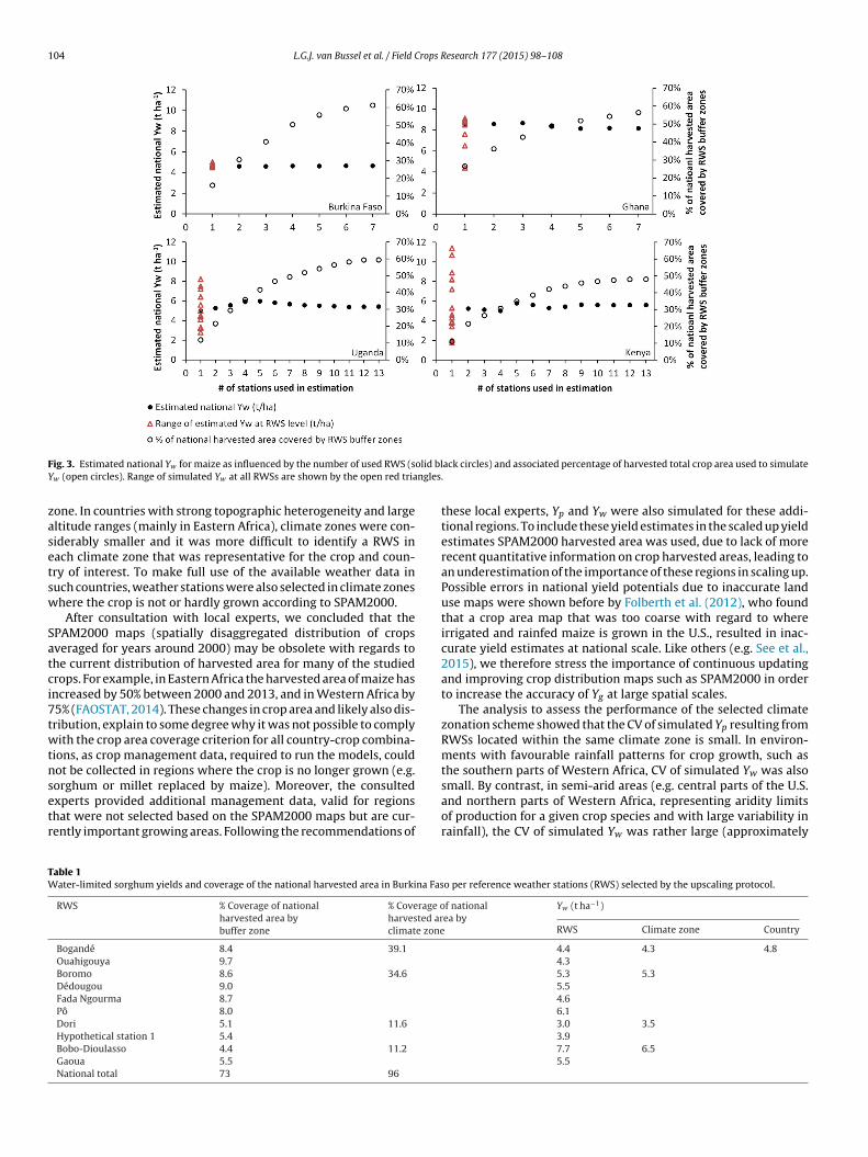

104 L.G.J. van Bussel et al. / Field Crops Research 177 (2015) 98–108

F olid blY ngles

zasetsw

Satci7twtnsetr

TW

ig. 3. Estimated national Yw for maize as influenced by the number of used RWS (sw (open circles). Range of simulated Yw at all RWSs are shown by the open red tria

one. In countries with strong topographic heterogeneity and largeltitude ranges (mainly in Eastern Africa), climate zones were con-iderably smaller and it was more difficult to identify a RWS inach climate zone that was representative for the crop and coun-ry of interest. To make full use of the available weather data inuch countries, weather stations were also selected in climate zoneshere the crop is not or hardly grown according to SPAM2000.

After consultation with local experts, we concluded that thePAM2000 maps (spatially disaggregated distribution of cropsveraged for years around 2000) may be obsolete with regards tohe current distribution of harvested area for many of the studiedrops. For example, in Eastern Africa the harvested area of maize hasncreased by 50% between 2000 and 2013, and in Western Africa by5% (FAOSTAT, 2014). These changes in crop area and likely also dis-ribution, explain to some degree why it was not possible to complyith the crop area coverage criterion for all country-crop combina-

ions, as crop management data, required to run the models, couldot be collected in regions where the crop is no longer grown (e.g.

orghum or millet replaced by maize). Moreover, the consultedxperts provided additional management data, valid for regionshat were not selected based on the SPAM2000 maps but are cur-ently important growing areas. Following the recommendations of

able 1ater-limited sorghum yields and coverage of the national harvested area in Burkina Fas

RWS % Coverage of nationalharvested area bybuffer zone

% Coverage oharvested arclimate zone

Bogandé 8.4 39.1Ouahigouya 9.7

Boromo 8.6 34.6Dédougou 9.0

Fada Ngourma 8.7

Pô 8.0

Dori 5.1 11.6Hypothetical station 1 5.4

Bobo-Dioulasso 4.4 11.2Gaoua 5.5

National total 73 96

ack circles) and associated percentage of harvested total crop area used to simulate.

these local experts, Yp and Yw were also simulated for these addi-tional regions. To include these yield estimates in the scaled up yieldestimates SPAM2000 harvested area was used, due to lack of morerecent quantitative information on crop harvested areas, leading toan underestimation of the importance of these regions in scaling up.Possible errors in national yield potentials due to inaccurate landuse maps were shown before by Folberth et al. (2012), who foundthat a crop area map that was too coarse with regard to whereirrigated and rainfed maize is grown in the U.S., resulted in inac-curate yield estimates at national scale. Like others (e.g. See et al.,2015), we therefore stress the importance of continuous updatingand improving crop distribution maps such as SPAM2000 in orderto increase the accuracy of Yg at large spatial scales.

The analysis to assess the performance of the selected climatezonation scheme showed that the CV of simulated Yp resulting fromRWSs located within the same climate zone is small. In environ-ments with favourable rainfall patterns for crop growth, such asthe southern parts of Western Africa, CV of simulated Yw was also

small. By contrast, in semi-arid areas (e.g. central parts of the U.S.and northern parts of Western Africa, representing aridity limitsof production for a given crop species and with large variability inrainfall), the CV of simulated Yw was rather large (approximately

o per reference weather stations (RWS) selected by the upscaling protocol.

f nationalea by

Yw (t ha−1)

RWS Climate zone Country

4.4 4.3 4.84.35.3 5.35.54.66.13.0 3.53.97.7 6.55.5

L.G.J. van Bussel et al. / Field Crops Research 177 (2015) 98–108 105

Table 2Water-limited sorghum yields and coverage of the national harvested area in Ethiopia per reference weather stations (RWS) selected by the upscaling protocol.

RWS % Coverage of nationalharvested area bybuffer zone

% Coverage of nationalharvested area byclimate zone

Yw (t ha–1)

RWS Climate zone Country

Dire Dawa 3.0 13.41 3.0 5.6 6.0Harar 3.1 8.3Kobo 0.1 2.8Melkassa 0.8 5.2Shire Endasilasse 3.8 5.5Hypothetical station 1 3.5 5.6Jijiga 0.4 10.72 2.3 2.3Assosa 1.5 7.09 7.9 7.4Gondar 0.2 4.1Kombolacha 0.1 5.29 3.9 8.1Woliso 0.9 9.7Wolkite 1.1 7.4Hypothetical station 2 0.6 5.00 5.9 5.9Ambo 1.3 4.26 7.5 7.5Gelemso 1.4 3.83 8.5 8.5Haramaya 1.2 2.91 8.0 8.0Nekemte 0.9 2.68 6.3 6.3Bahir Dar 0.0 2.33 5.1 5.1Mekele 1.4 1.84 2.6 2.6Ayira 0.8 1.68 8.1 8.1Butajira 0.5 1.34 6.0 6.0Gore 0.2 1.28 9.6 9.6Pawe 0.2 0.25 5.3 5.3Shambu 0.1 0.20 10.2 10.2National total 27% 64%

Table 3Percentage of national harvested area covered by buffer zones of the selected RWS in ten African countries, when following the protocol as much as possible. In parenthesesthe percentage of selected RWS that cover <1% of national harvested area, blank cells indicate that this country/crop combination had less than 100,000 ha (criteria to besimulated).

Country/crop Rainfed maize (%) Rainfed wheat (%) Rainfed sorghum (%) Rainfed millet (%) Rainfed rice (%) Irrigated rice (%)

Mali 35 (0) 35 (13) 51 (38) 57 (0) 59 (0)Niger 54 (0) 51 (0) 17 (0)Burkina Faso 61 (0) 73 (0) 75 (0) 48 (0) 59 (0)Nigeria 27 (44) 39 (0) 34 (0) 25 (0) 25 (0)Ghana 56 (0) 74 (0) 75 (0) 40 (0) 22 (0)Ethiopia 22 (68) 26 (25) 27 (64) 26 (65)Kenya 49 (29) 28 (43) 31 (67) 27 (50)Uganda 61 (7) 65 (18) 68 (9) 53 (33)Tanzania 30 (44) 44 (0) 45 (0) 55 (9) 16 (0) 13 (0)Zambia 26 (55) 18 (57) 34 (0)

Table 4Percentage of national harvested area covered by the selected climate zones in ten African countries when following the protocol as much as possible. In parentheses thepercentage of selected climate zones that cover <5% of national harvested area, blank cells indicate that this country/crop combination had less than 100,000 ha (criteria tobe simulated).

Country/crop Rainfed maize (%) Rainfed wheat (%) Rainfed sorghum (%) Rainfed millet (%) Rainfed rice (%) Irrigated rice (%)

Mali 59 (0) 81 (25) 96 (25) 83 (0) 84 (0)Niger 97 (0) 94 (0) 71 (50)Burkina Faso 75 (0) 96 (0) 99 (0) 65 (0) 90 (0)Nigeria 65 (50) 78 (22) 79 (38) 46 (17) 53 (17)Ghana 87 (0) 90 (0) 90 (0) 55 (0) 57 (0)Ethiopia 58 (64) 52 (44) 64 (75) 45 (83)Kenya 56 (60) 36 (50) 53 (60) 49 (50)Uganda 77 (14) 74 (14) 76 (0) 78 (0)Tanzania 72 (29) 51 (25) 74 (20) 78 (0) 41 (50) 37 (0)Zambia 85 (20) 90 (0) 50 (0)

Table 5Number of selected climate zones, number of selected RWS per climate zone, and the area-weighted CV (among RWS) for Yp and Yw within each zone.

Country/region and crop Number of selectedclimate zones

Number of RWS Area-weighted CV (%)

Average per climate zone Minimum in a zone Maximum in a zone Yp Yw

U.S.—maize 28 6.8 3 25 5 19Germany—winter wheat 8 5.6 3 8 4 8Western Africa—sorghum 8 7.8 3 21 7 23

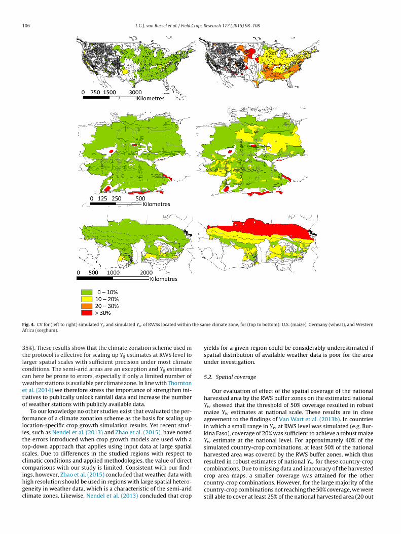
106 L.G.J. van Bussel et al. / Field Crops Research 177 (2015) 98–108

F the saA

3tlccweto

flittsccihgc

ig. 4. CV for (left to right) simulated Yp and simulated Yw of RWSs located within

frica (sorghum).

5%). These results show that the climate zonation scheme used inhe protocol is effective for scaling up Yg estimates at RWS level toarger spatial scales with sufficient precision under most climateonditions. The semi-arid areas are an exception and Yg estimatesan here be prone to errors, especially if only a limited number ofeather stations is available per climate zone. In line with Thornton

t al. (2014) we therefore stress the importance of strengthen ini-iatives to publically unlock rainfall data and increase the numberf weather stations with publicly available data.

To our knowledge no other studies exist that evaluated the per-ormance of a climate zonation scheme as the basis for scaling upocation-specific crop growth simulation results. Yet recent stud-es, such as Nendel et al. (2013) and Zhao et al. (2015), have notedhe errors introduced when crop growth models are used with aop-down approach that applies using input data at large spatialcales. Due to differences in the studied regions with respect tolimatic conditions and applied methodologies, the value of directomparisons with our study is limited. Consistent with our find-

ngs, however, Zhao et al. (2015) concluded that weather data withigh resolution should be used in regions with large spatial hetero-eneity in weather data, which is a characteristic of the semi-aridlimate zones. Likewise, Nendel et al. (2013) concluded that crop

me climate zone, for (top to bottom): U.S. (maize), Germany (wheat), and Western

yields for a given region could be considerably underestimated ifspatial distribution of available weather data is poor for the areaunder investigation.

5.2. Spatial coverage

Our evaluation of effect of the spatial coverage of the nationalharvested area by the RWS buffer zones on the estimated nationalYw showed that the threshold of 50% coverage resulted in robustmaize Yw estimates at national scale. These results are in closeagreement to the findings of Van Wart et al. (2013b). In countriesin which a small range in Yw at RWS level was simulated (e.g. Bur-kina Faso), coverage of 20% was sufficient to achieve a robust maizeYw estimate at the national level. For approximately 40% of thesimulated country-crop combinations, at least 50% of the nationalharvested area was covered by the RWS buffer zones, which thusresulted in robust estimates of national Yw for these country-cropcombinations. Due to missing data and inaccuracy of the harvested

crop area maps, a smaller coverage was attained for the othercountry-crop combinations. However, for the large majority of thecountry-crop combinations not reaching the 50% coverage, we werestill able to cover at least 25% of the national harvested area (20 out

rops R

oseFttcnwl

metmemgrsiq

mavwuaamatg

6

afwtzrhSaticl

sfbu

A

GUtGi

L.G.J. van Bussel et al. / Field C

f 27). A coverage of only 25% could introduce some errors in thecaled up Yw estimates, especially for countries in which the Yw

stimates at RWS level show a large range (e.g. maize in Kenya,ig. 3). However, the magnitude of that error was limited for maizeo 1 t ha−1 for 3 out of the 4 studied countries. When consideringhe coverage by climate zones, only for 5 out of 44 country-cropombinations a coverage of less than 50% was attained. In combi-ation with the demonstrated robustness of the climate zonation,e conclude that in general the scaled-up Yg estimates at national

evel are sufficiently accurate.Recent research showed the uncertainty in global gridded crop

odels for climate change impacts on agriculture (Rosenzweigt al., 2014). The authors indicated this uncertainty was mainly dueo differences in structure and implementation of the applied crop

odels and assumptions made about agricultural management,.g. input quantities. Uncertainties related to their applied scalingethods, in which site-based crop models were run with global

ridded weather data, were not quantified nor discussed. The cur-ent study could quantify the error and uncertainty in the nationalcale results from the applied scaling methods. Hence, the upscal-ng approach and analysis developed and described here could helpuantify such uncertainty for large-scale crop model studies.

To increase understanding about spatial variability within cli-ate zones and scaled up Yg estimates based on the bottom-up

pproach described in this paper, future work should focus onariability in soil properties, especially properties influencing soilater holding capacity and rooting depth, and their effects on

pscaled Yg estimates. The issue of examining rainfall data char-cteristics and effects of different rainfall data quality on resultslso needs to be studied. Finally, increased efforts to collect andake publicly available good quality weather, soil, and crop man-

gement data in regions with substantial harvested area that lackhese data would have large payoffs for improving quality of yieldap estimates in SSA.

. Concluding remarks

This study shows that the proposed protocol developed andpplied in the Global Yield Gap Atlas project is reasonably robustor scaling up Yg estimates to regional and national levels based on

eather station data supplemented by local soil and cropping sys-em data. This conclusion was based on an evaluation of the climateonation scheme, which appeared to be accurate enough to achieveobust Yg estimates at larger spatial areas and sufficient coverage ofarvested crop area by the protocols for selecting weather stations.emi-arid areas with large variability in rainfall are an exceptionnd here scaled up water-limited yield gap estimates can be proneo errors, especially if only a limited number of weather stationss available per climate zone. In addition, in some heterogeneousountries data availability hindered full application of the protocol,eading to possible errors in the scaled up yield gap estimates.

We found that global crop area distribution maps are still aource of error for selecting relevant locations for data collectionor Yg estimates. Continuous updating and improving of crop distri-ution maps is essential, and should be complemented with localp-to-date knowledge about crop area distribution.

cknowledgements

Support for this research was provided by the Bill and Melindaates Foundation, the Daugherty Water for Food, Institute at the

niversity of Nebraska—Lincoln and Wageningen University. We

hank the country agronomists contributing to the Global Yieldap Atlas for providing weather and management data, includ-

ng Dr. Korodjouma Ouattara (Institut del’Environnement et de

esearch 177 (2015) 98–108 107

Recherches agricoles, Burkina Faso), Dr. Mamoutou Kouressy (Insti-tute of Rural Economy, Mali), Dr. Abdullahi Bala (Federal Universityof Technology, Minna, Nigeria), Dr. Samuel Adjei-Nsiah (Universityof Ghana, Ghana), Dr. Agali Alhassane (Centre Regional AGRHYMET,Niger), Dr. Kindie Tesfaye (CIMMYT, Ethiopia), Dr. Ochieng Adimo(Jomo Kenyatta University of Agriculture and Technology, Kenya),Dr. Joachim Makoi (Ministry of Agriculture Food Security andCooperatives, Tanzania), Dr. Kayuki Kaizzi (National AgricultureResearch Laboratories, Uganda), and Dr. Regis Chikowo (Univer-sity of Zimbabwe, Zimbabwe) as well as valuable discussions ofthe results. Discussions with Pepijn van Oort (Africa Rice Centerand Wageningen University) and René Schils (Wageningen Univer-sity) and comments of two anonymous reviewers are also highlyappreciated.

References

Alexandratos, N., Bruinsma, J., 2012. World Agriculture towards 2030/2050: The2012 Revision. FAO, Food and Agriculture Organization of the United Nations.

Baron, C., Sultan, B., Balme, M., Sarr, B., Traoré, S., Lebel, T., Janicot, S., Dingkuhn, M.,2005. From GCM grid cell to agricultural plot: scale issues affecting modellingof climate impact. Philos. Trans. R. Soc. London, Ser. B 360, 2095–2108.

Batjes, N.H., 2012. ISRIC-WISE Derived Soil Properties on a 5 by 5 arc-minutes GlobalGrid (Ver. 1.2). ISRIC—World Soil Information, Wageningen, pp. 57.

Bierkens, M.F.P., Finke, P.A., 2000. Upscaling and Downscaling Methods for Environ-mental Research. Kluwer, Dordrecht, The Netherlands.

Bouman, B.A.M., Kropff, M.J., Tuong, T.P., Wopereis, M.C.S., Ten Berge, H.F.M., VanLaar, H.H., 2001. ORYZA2000: Modeling Lowland Rice. IRRI, Los Banos.

Brus, D.J., 1994. Improving design-based estimation of spatial means by soil mapstratification. A case study of phosphate saturation. Geoderma 62, 233–246.

Cassman, K.G., 1999. Ecological intensification of cereal production systems: yieldpotential, soil quality, and precision agriculture. Proc. Nat. Acad. Sci. U.S.A. 96,5952–5959.

Challinor, A.J., Parkes, B., Ramirez-Villegas, J., 2015. Crop yield response to climatechange varies with cropping intensity. Global Change Biol. 21 (4), 1679–1688.

Evans, L.T., 1993. Crop Evolution, Adaptation and Yield. Cambridge University Press,Cambridge.

Ewert, F., Van Ittersum, M.K., Heckelei, T., Therond, O., Bezlepkina, I., Andersen, E.,2011. Scale changes and model linking methods for integrated assessment ofagri-environmental systems. Agric. Ecosyst. Environ. 142, 6–17.

FAOSTAT, 2014. 〈http://faostat3.fao.org/home/E〉 (accessed at: 19-10-2014).Folberth, C., Yang, H., Wang, X., Abbaspour, K.C., 2012. Impact of input data resolution

and extent of harvested areas on crop yield estimates in large-scale agriculturalmodeling for maize in the USA. Ecol. Model. 235–236, 8–18.

Grassini, P., Van Bussel, L.G.J., Van Wart, J., Wolf, J., Claessens, L., Yang, H., Boogaard,H., De Groot, H., Van Ittersum, M.K., Cassman, K.G., 2015. How good is goodenough? Data requirements for reliable yield-gap analysis. Field Crops Res.

Heuvelink, G.B.M., Pebesma, E.J., 1999. Spatial aggregation and soil process mod-elling. Geoderma 89, 47–65.

Hijmans, R.J., Cameron, S.E., Parra, J.L., Jones, P.G., Jarvis, A., 2005. Very high res-olution interpolated climate surfaces for global land areas. Int. J. Climatol. 25,1965–1978.

Mitchell, T.D., Jones, P.D., 2005. An improved method of constructing a databaseof monthly climate observations and associated high-resolution grids. Int. J.Climatol. 25, 693–712.

National Oceanic and Atmospheric Association, 2014. 〈ftp://ftp.ncdc.noaa.gov/pub/data/gsod/〉 and 〈http://www.ncdc.noaa.gov/oa/climate/ghcn-daily/〉(accessed at: 18-11-2014).

Nendel, C., Wieland, R., Mirschel, W., Specka, X., Guddat, C., Kersebaum, K.C., 2013.Simulating regional winter wheat yields using input data of different spatialresolution. Field Crop Res. 145, 67–77.

Portmann, F.T., Siebert, S., Doll, P., 2010. MIRCA2000-Global monthly irrigated andrainfed crop areas around the year 2000: a new high-resolution data set foragricultural and hydrological modeling. Global Biogeochem. Cycles 24, GB1011.

Ramirez-Villegas, J., Challinor, A., 2012. Assessing relevant climate data for agricul-tural applications. Agric. For. Meteorol. 161, 26–45.

Rosenzweig, C., Elliott, J., Deryng, D., Ruane, A.C., Müller, C., Arneth, A., Boote, K.J., Fol-berth, C., Glotter, M., Khabarov, N., Neumann, K., Piontek, F., Pugh, T.A.M., Schmid,E., Stehfest, E., Yang, H., Jones, J.W., 2014. Assessing agricultural risks of climatechange in the 21st century in a global gridded crop model intercomparison. Proc.Nat. Acad. Sci. U.S.A. 111, 3268–3273.

See, L., Fritz, S., You, L., Ramankutty, N., Herrero, M., Justice, C., Becker-Reshef, I.,Thornton, P., Erb, K., Gong, P., Tang, H., van der Velde, M., Ericksen, P., McCal-lum, I., Kraxner, F., Obersteiner, M., 2015. Improved global cropland data as anessential ingredient for food security. Global Food Secur. 4, 37–45.

Simpson, J., Kummerow, C., Tao, W.K., Adler, R.F., 1996. On the tropical rainfall

measuring mission (TRMM). Meteorol. Atmos. Phys. 60, 19–36.

Stackhouse, P.W., 2014. Prediction of Worldwide Energy Resources,〈http://power.larc.nasa.gov〉 (accessed at: 18-11-2014).

Supit, I., van Diepen, C.A., de Wit, A.J.W., Wolf, J., Kabat, P., Baruth, B., Ludwig, F.,2012. Assessing climate change effects on European crop yields using the crop

1 rops R

T

V

V

V

V

V

V

V

V

08 L.G.J. van Bussel et al. / Field C

growth monitoring system and a weather generator. Agric. For. Meteorol. 164,96–111.

hornton, P.K., Ericksen, P.J., Herrero, M., Challinor, A.J., 2014. Climate variability andvulnerability to climate change: a review. Global Change Biol. 20, 3313–3328.

an Bussel, L.G.J., Müller, C., Van Keulen, H., Ewert, F., Leffelaar, P.A., 2011. The effectof temporal aggregation of weather input data on crop growth models’ results.Agric. For. Meteorol. 151, 607–619.

an Delden, H., Van Vliet, J., Rutledge, D.T., Kirkby, M.J., 2011. Comparison of scaleand scaling issues in integrated land-use models for policy support. Agric.,Ecosyst. Environ. 142, 18–28.

an Ittersum, M.K., Cassman, K.G., Grassini, P., Wolf, J., Tittonell, P., Hochman, Z.,2013. Yield gap analysis with local to global relevance—a review. Field Crop Res.143, 4–17.

an Oort, P.A., De Vries, M.E., Yoshida, H., Saito, K., 2015. Improved climaterisk simulations for rice in arid environments. PLoS One. 10 (3), e0118114,http://dx.doi.org/10.1371/journal.pone.0118114.

an Oort, P.A.J., Saito, K., Zwart, S.J., Shrestha, S., 2014. A simple model for simulatingheat induced sterility in rice as a function of flowering time and transpirationalcooling. Field Crop Res. 156, 303–312.

an Wart, J., Grassini, P., Cassman, K.G., 2013a. Impact of derived global weatherdata on simulated crop yields. Global Change Biol. 19, 3822–3834.

an Wart, J., Grassini, P., Yang, H.S., Claessens, L., Jarvis, A., Cassman, K.G., 2015.Creating long-term weather data from the thin air for crop simulation mod-

elling. Agric. For. Meteorol., http://dx.doi.org/10.1016/j.agrformet.2015.02.020(In press).

an Wart, J., Kersebaum, K.C., Peng, S., Milner, M., Cassman, K.G., 2013b. Estimat-ing crop yield potential at regional to national scales. Field Crop Res. 143,34–43.

esearch 177 (2015) 98–108

Van Wart, J., van Bussel, L.G.J., Wolf, J., Licker, R., Grassini, P., Nelson, A., Boogaard, H.,Gerber, J., Mueller, N.D., Claessens, L., van Ittersum, M.K., Cassman, K.G., 2013c.Use of agro-climatic zones to upscale simulated crop yield potential. Field CropRes. 143, 44–55.

Wang, E., Cresswell, H., Bryan, B., Glover, M., King, D., 2009. Modelling farming sys-tems performance at catchment and regional scales to support natural resourcemanagement. NJAS—Wageningen J. Life Sci. 57, 101–108.

Wolf, J., Hessel, R., Boogaard, H.L., De Wit, A., Akkermans, W., Van Diepen, C.A., 2011.Modeling winter wheat production over Europe with WOFOST—the effect of twonew zonations and two newly calibrated model parameter sets. In: Ahuja, L.R.,Ma, L. (Eds.), Methods of Introducing System Models into Agricultural Research.Advances in Agricultural Systems Modeling. 2: Trans-disciplinary Research,Synthesis, and Applications. ASA–SSSA–CSSA Book Series. ASA–SSSA–CSSA, pp.297–326.

Wolf, J., Van Diepen, C.A., 1995. Effects of climate change on grain maize yieldpotential in the European community. Clim. Chang. 29, 299–331.

Yang, H., Dobermann, A., Cassman, K.G., Walters, D.T., 2006. Features, applica-tions, and limitations of the hybrid-maize simulation model. Agron. J. 98,737–748.

You, L., Crespo, S., Guo, Z., Koo, J., Sebastian, K., Tenorio, M.T., Wood, S., Wood-Sichra,U., 2009. Spatial Production Allocation Model (SPAM) 2000 Version 3 Release 6,〈http://mapspam.info/〉.

You, L., Wood, S., Wood-Sichra, U., 2006. Generating global crop maps: from census

to grid. In: IAAE (International Association of Agricultural Economists), AnnualConference, Gold Coast, Australia.

Zhao, G., Siebert, S., Enders, A., Rezaei, E.E., Yan, C., Ewert, F., 2015. Demand formulti-scale weather data for regional crop modeling. Agric. For. Meteorol. 200,156–171.

Creating long-term weather data from thin air for crop simulation

modelling

Justin Van Wart, Patricio Grassini, Haishun Yang, Lieven Claessens, Andy Jarvis, Kenneth G. Cassman

2015, Agricultural and Forest Meteorology, Volumes 209-210: 49-58

http://www.sciencedirect.com/science/article/pii/S0168192315000696

Cs

JAa

b

c

d

a

ARRA

KYYWC

1

dm

RTo

h0

Agricultural and Forest Meteorology 208 (2015) 49–58

Contents lists available at ScienceDirect

Agricultural and Forest Meteorology

j our na l ho me page: www.elsev ier .com/ locate /agr formet

reating long-term weather data from thin air for cropimulation modeling

ustin Van Wart a, Patricio Grassini a,∗, Haishun Yang a, Lieven Claessens b,c,ndrew Jarvis d, Kenneth G. Cassman a

Department of Agronomy and Horticulture, University of Nebraska-Lincoln, Lincoln, NE 68583-0915, USAInternational Crops Research Institute for the Semi-Arid Tropics (ICRISAT), P.O. Box 39063, 00623 Nairobi, KenyaSoil Geography and Landscape Group, Wageningen University, P.O. Box 47, 6700 AA Wageningen, The NetherlandsInternational Center for Tropical Agriculture (CIAT), Apartado Aéreo 6713, Cali, Colombia

r t i c l e i n f o

rticle history:eceived 4 June 2014eceived in revised form 18 February 2015ccepted 28 February 2015

eywords:ield potentialeild variabilityeather data

rop simulation model

a b s t r a c t

Simulating crop yield and yield variability requires long-term, high-quality daily weather data, includingsolar radiation, maximum (Tmax) and minimum temperature (Tmin), and precipitation. In many regions,however, daily weather data of sufficient quality and duration are not available. To overcome this limita-tion, we evaluated a new method to create long-term weather series based on a few years of observed dailytemperature data (hereafter called propagated data). The propagated data are comprised of uncorrectedgridded solar radiation from the Prediction of Worldwide Energy Resource dataset from the NationalAeronautics and Space Administration (NASA–POWER), rainfall from the Tropical Rainfall MeasuringMission (TRMM) dataset, and location-specific calibration of NASA–POWER Tmax and Tmin using a limitedamount of observed daily temperature data. The distributions of simulated yields of maize, rice, or wheatwith propagated data were compared with simulated yields using observed weather data at 18 sites inNorth and South America, Europe, Africa, and Asia. Other sources of weather data typically used in cropmodeling for locations without long-term observed weather data were also included in the comparison:(i) uncorrected NASA–POWER weather data and (ii) generated weather data using the MarkSim weathergenerator. Results indicated good agreement between yields simulated with propagated weather dataand yields simulated using observed weather data. For example, the distribution of simulated yieldsusing propagated data was within 10% of the simulated yields using observed data at 78% of locationsand degree of yield stability (quantified by coefficient of variation) was very similar at 89% of locations. In

contrast, simulated yields based entirely on uncorrected NASA–POWER data or generated weather datausing MarkSim were within 10% of yields simulated using observed data in only 44 and 33% of cases,respectively, and the bias was not consistent across locations and crops. We conclude that, for most loca-tions, 3 years of observed daily Tmax and Tmin data would allow creation of a robust weather data set forsimulation of long-term mean yield and yield stability of major cereal crops.

© 2015 Z. Published by Elsevier B.V. This is an open access article under the CC BY-NC-ND license

. Introduction

Due to year-to-year fluctuation in weather patterns, long-termaily weather data, including solar radiation, temperature (maxi-um [Tmax] and minimum [Tmin]), and precipitation, are required

Abbreviations: GridWD, gridded weather data; GenWD, generated weather data;H, relative humidity; Tmin, minimum temperature; Tmax, maximum temperature;dew, dew point temperature; ETo, grass-based reference evapotranspiration; OWD,bserved weather data; PWD, propagated weather data.∗ Corresponding author. Tel.: +1 4024725554.

E-mail address: pgrassini2@unl.edu (P. Grassini).

ttp://dx.doi.org/10.1016/j.agrformet.2015.02.020168-1923/© 2015 Z. Published by Elsevier B.V. This is an open access article under the C

(http://creativecommons.org/licenses/by-nc-nd/4.0/).

to estimate crop yield potential and its variability using crop sim-ulation models (Whisler et al., 1986; Boote et al., 1996; van Busselet al., 2011 Van Wart et al., 2013a). Such estimates of yield poten-tial and its variability are essential for analysis of food security,assessing impact of climate change on crop production, develop-ment and use of crop management decision-support tools, andto support and target agronomic research and policy. Dependingon the degree of weather variability among years, at least 10–20years of daily weather data are necessary for reliable estimates of

mean yield potential and its inter-annual variability (van Ittersumet al., 2013 ; Van Wart et al. 2013a; Grassini et al., 2015). In manyparts of the world, however, most weather stations only have afew years of daily weather records available and often not all of

C BY-NC-ND license (http://creativecommons.org/licenses/by-nc-nd/4.0/).

5 d Fore

t(loidfis

(wtcwcsGy

wmuTdtisaftea

TSS

n

h

I

0 J. Van Wart et al. / Agricultural an

he variables necessary for crop model simulations are measurede.g., incident solar radiation). Unfortunately, many regions withimited availability of weather data (e.g., Sub-Saharan Africa) aref greatest concern with regard to food security and vulnerabil-

ty to climate change (Lobell et al., 2008). Hence, it is important toevelop methods for generating reliable, long-term weather data

or these regions where availability of weather data severely lim-ts ability to perform robust assessments of yield gaps, and foodecurity scenarios.

Gridded weather data (GridWD) or generated weather dataGenWD) have been used as alternatives in regions where observedeather data (OWD) are not available (Table 1). Crop simula-

ion studies relying on GridWD and GenWD, however, have rarelyompared simulated yields against simulations using OWD fromeather stations located within the area of study. However, this is

rucial because, in generating long-term weather data with globalpatial coverage, sources of error can be incorporated into bothridWD and GenWD that can result in biased estimates of cropield and its variability over time.

GridWD are typically derived by interpolation of observedeather data over space, or may also be derived from global climateodels, to estimate daily or monthly weather data for each individ-

al grid cell of land area (Kanamitsu et al., 2002; New et al., 2002).he quality of the estimation for a given grid cell depends on theensity and distribution of the weather stations used in its deriva-ion. Because both density and distribution are far from satisfactoryn many regions of the world, derived GridWd in these regions areubject to a large degree of uncertainty. In fact, even in regions withn adequate density of weather stations, poor agreement has beenound between simulated crop yields using GridWD versus simula-

ions using OWD from a location within the same grid cell (Mearnst al., 2001; Baron et al., 2005). Regardless of whether the GridWDre derived through interpolation or from climate models, the bias

able 1tudies that used gridded or generated weather data for agricultural research inub-Saharan Africa.

Database References

Gridded weather dataCRUa (Fischer et al., 2002; Foley et al., 2005;

Bondeau et al., 2007; Lobell, 2007;Lobell et al., 2008; Battisti and Naylor2009; Licker et al., 2010; Folberth et al.,2012; Folberth et al., 2013)

NASAb (Folberth et al., 2012; Arndt et al.,2012)

NCEPc (Lobell and Asner 2003; Nemani et al.,2003; Bagley et al., 2012)

WorldClimd (Thornton et al., 2009; Nelson et al.,2010; Claessens et al., 2012)

Othere (Jones and Thornton, 2003; Stéphenneand Lambin, 2001; Lobell et al., 2008;Rowhani et al., 2011)

Weather generatorsMarkSim (Mavromatis and Hansen, 2001; Jones

and Thornton, 2003; Thornton et al.,2009; Claessens et al., 2012)

WGEN (WeatherMan) (Mavromatis and Hansen, 2001; Liet al., 2005; Schuol et al., 2008)

ClimGen (Abraha and Savage, 2006; Laux et al.,2010)

a Climate Research Unit (CRU) http://badc.nerc.ac.uk/data/cru/.b National Aeronautics and Space Administration (NASA) http://power.larc.

asa.gov/.c National Center for Environmental Prediction/Department of Energy (NCEP)

ttp://www.esrl.noaa.gov/psd/data/gridded/data.ncep.reanalysis2.html.d WorldClim http://www.worldclim.org/.e All future climate data as modeled by global climate models, distributed by the

nternational Panel on Climate Change (IPCC) http://www.ipcc-data.org/.

st Meteorology 208 (2015) 49–58

in simulated yields using GridWD, relative to yields simulated usingOWD, has been found to be unpredictable and inconsistent, havingdifferent sign and magnitude across locations for temperature andrainfall (Van Wart et al., 2013b).

A stochastic weather generator produces synthetic time seriesof daily weather data (GenWD) for as many years as specifiedfor a location based on the statistical characteristics of historicaldaily or monthly OWD at that location (Hutchinson, 1987; Jonesand Thornton, 2000; Hansen and Mavromatis, 2001; Mavromatisand Hansen, 2001). Models for generating stochastic weather dataare typically developed in two steps: the first step is to modeldaily precipitation and the second step is to model or estimate theremaining variables of interest, such as daily Tmax and Tmin, solarradiation, humidity and wind speed. Even when decades of dailyOWD are used to calibrate weather generators, they may performpoorly when compared to simulated crop yields based on OWDand typically underestimate inter-annual variation in crop modelsimulations (Semenov and Porter, 1995; Hammer et al., 2002). Like-wise, though monthly means and variances of GenWD and OWDmay be similar, short periods of extreme events, which are ofparticular importance for crop growth, yield and even crop fail-ure, are typically not well represented in generated data (Kyselyand Dubrovsky, 2005; Semenov, 2008). While there are continuingefforts to improve weather generators, such efforts are constrainedby the number of years and sites required for their parameterization(Baigorria and Jones, 2010; Rosenzweig et al., 2013).

Daily OWD with sufficient number of years to simulate long-term average crop yield and its variability (>10 years) are notavailable for many regions of the world. In contrast, short-termOWD of several years duration (typically <5 years) with daily max-imum and minimum temperature (Tmax and Tmin, respectively) isoften available for most regions. For example, in Africa there are atotal of 1048 meteorological stations reporting at least 3 years ofpublically available weather data, but less than 12% of these sta-tions have at least 15 years of OWD of adequate quality (missing<10% of total data and with no more than 30 data days missingconsecutively) for crop simulation (National Climate Data Center,2014). As an alternative to the use of GridWD or GenWD, here wepresent a protocol that utilizes 3 years of observed Tmax and Tmindata, combined with long-term GridWD of solar radiation and pre-cipitation, to generate a long-term daily weather data set suitablefor simulation of crop yields (hereafter called ‘propagated’ weatherdata [PWD]). The purpose of this paper is to evaluate how simulatedyields compare when using PWD versus (i) OWD, (ii) GridWD and(iii) GenWD. In the present paper, the comparison was made across18 sites, located in four continents (Europe, Asia, America, andAfrica), for which long-term, high-quality daily OWD were avail-able. Simulated crops include three major cereals (maize, rice andwheat), each simulated with well-validated crop models and basedon site-specific soil properties and crop management to ensureagronomic relevance.

2. Materials and methods

2.1. Evaluation of NASA gridded data

The Prediction of Worldwide Energy Resource (POWER) datasetfrom the National Aeronautics and Space Administration (NASA,2012), hereafter called NASA, was selected as the GridWD source foruse in this study because it is publically accessible, shows generalacceptable agreement with ground data for incident solar radia-

tion, and has been used in previous studies that have simulatedcrop yields (Bai et al., 2010 Van Wart et al., 2013a,b). The NASAdataset contains daily incident solar radiation, Tmax, Tmin, dew pointtemperature (Tdew), precipitation, wind speed, and relative humid-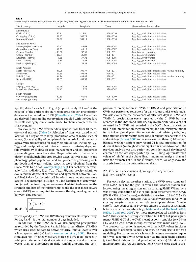

J. Van Wart et al. / Agricultural and Forest Meteorology 208 (2015) 49–58 51

Table 2Meteorological station name, latitude and longitude (in decimal degrees), years of available weather data, and measured weather variables.

Site & country Latitude Longitude Years Measured weather variables

Eastern AsiaGushi (China) 32.1 115.4 1990–2010 Tmin, Tmax, radiation, precipitationChongqing (China) 29.35 106.28 1990–2010 Tmin, Tmax, radiation, precipitationNanning (China) 22.38 108.13 1990–2010 Tmin, Tmax, radiation, precipitation

Sub-Saharan AfricaDedougou (Burkina Faso) 12.47 −3.48 1998–2007 Tmin, Tmax, radiation, precipitationGaoua (Burkina Faso) 10.33 −3.18 1998–2007 Tmin, Tmax, radiation, precipitationChapata (Zambia) −13.56 32.59 1998–2011 Tmin, Tmax, precipitationChoma (Zambia) −16.81 26.97 1998–2011 Tmin, Tmax, precipitationKatumani (Kenya) −1.55 37.32 1998–2005 Tmin, Tmax, precipitationEmbu (Kenya) −0.54 37.45 1998–2007 Tmin, Tmax, precipitationMelkassa (Ethiopia) 8.4 39.33 1998–2005 Tmin, Tmax, radiation, precipitation

North AmericaNorth Platte (USA) 41.08 −100.77 1998–2011 Tmin, Tmax, radiation, precipitation, relative humidityMead (USA) 41.25 −96.58 1998–2011 Tmin, Tmax, radiation, precipitationDekalb (USA) 41.84 −88.85 1998–2011 Tmin, Tmax, radiation, precipitation, relative humidityBondville (USA) 40.05 −88.37 1998–2011 Tmin, Tmax, radiation, precipitation

EuropeLeipzig (Germany) 51.48 12.28 1998–2007 Tmin, Tmax, radiation, precipitationDusseldorf (Germany) 51.43 6.77 1998–2007 Tmin, Tmax, radiation, precipitation

iedaEt

olwlT(supiGaealtseb

R

wf

awastw

South AmericaOliveros (Argentina) −32.33 −60.51

Balcarce (Argentina) −37.8 −58.3

ty (RH) data for each 1◦ × 1◦ grid (approximately 111 km2 at thequator) of the entire globe starting in 1983, though precipitationata are not reported until 1997 (Chandler et al., 2004). These datare derived from satellite observations coupled with the Goddardarth Observing System climate model to obtain complete terres-rial coverage.

We evaluated NASA weather data against OWD from 18 mete-rological stations (Table 2). Selection of sites was based on (i)

ocation in a region with large production area of maize, rice, orheat, (ii) availability of complete daily records for all meteoro-

ogical variables required for crop yield simulation, including Tmin,max and precipitation, with few erroneous or missing days, andiii) availability of data on crop management and soil propertiesurrounding each weather station. Required inputs to run crop sim-lation models, including crop sowing dates, cultivar maturity andhenology, plant population, and soil properties governing root-

ng depth and water holding capacity, were obtained from thelobal Yield Gap Atlas (www.yieldgap.org). For each weather vari-ble (solar radiation, Tmax, Tmin, Tdew, RH, and precipitation), wevaluated the degree of correlation and agreement between OWDnd NASA data for the grid cell in which weather stations wereocated. The intercept (b), slope (m), and coefficient of determina-ion (r2) of the linear regression were calculated to determine thetrength and bias of the relationship, while the root mean squarerror (RMSE) was computed to measure the degree of agreementetween data sources:

MSE =

√√√√√

n∑

i=1

(xi − yi)2

n(1)

here xi and yi are NASA and OWD for a given variable, respectively,or day i and n is the total number of days included.

In addition to the NASA data, we also analyzed precipitations recorded by the Tropical Rainfall Measuring Mission (TRMM),hich uses satellite data to derive historical rainfall events over

finer spatial grid (∼5 km2) (Kummerow et al., 2000). Becauseimulated non-irrigated yields are more sensitive to differences inotal precipitation and its distribution during a period of severaleeks than to differences in daily rainfall amounts, the com-

1998–2009 Tmin, Tmax, radiation, precipitation1998–2010 Tmin, Tmax, radiation, precipitation

parison of precipitation in NASA or TRMM and precipitation inOWD was performed separately for daily values and 2-week totals.We also evaluated the prevalence of false wet days in NASA andTRMM (a precipitation event reported by the GridWD but notrecorded in the OWD) and false dry days (a precipitation event notreported by GridWD but recorded in the OWD). Due to uncertain-ties in the precipitation measurements and the relatively minorimpact of very small precipitation events on simulated yields, onlyprecipitation events >6 mm were considered for the analysis of dryand wet days (Sadras, 2003 and references cited therein). Moreover,because weather stations may record 24-h total precipitation fordifferent times (midnight-to-midnight versus noon-to-noon), theprevious analysis was also performed considering a 3-day intervalcentered on the wet day reported by OWD. Using log-transformedvalues of rainfall in the above linear regression analysis changedlittle the estimates of b, m and r2 values, hence, we only show theanalysis based on the untransformed data.

2.2. Creation and evaluation of propagated and generatedlong-term weather records

For each selected weather station, the OWD were comparedwith NASA data for the grid in which the weather station waslocated using linear regression and calculating RMSE. When therewas strong correlation (r2 > 0.7) and good agreement with OWD(RMSE <30% of OWD mean), with little bias (m from 0.8 to 1.2, b < 2%of OWD mean), NASA data for that variable were used directly forcreating long-term weather records for crop simulation. Similarcutoffs have been used in previous studies to assess associationsbetween weather variables (e.g., Mahmood and Hubbard, 2002;Hubbard and You, 2005). For those meteorological variables fromNASA that exhibited strong correlation (r2 > 0.7) but poor agree-ment (RMSE >30% of the OWD mean) or consistent bias (m < 0.8 or>1.2 and b > 2% of OWD mean), correction was made using OWD.The previous correction is needed to bring NASA values in closeragreement to observed values, and thus, be more useful for crop

modelling. For correction of each variable, a linear regression equa-tion was generated with OWD taken as the dependent variable(y) and NASA data as the independent variable (x). The slope andintercept from the regression equation y = mx + b were used to pro-

5 d Fore

ddvsrit

aOtstiTpest1wro

laClSmn2fOSwso

safid

TS(T

2 J. Van Wart et al. / Agricultural an

uce a corrected estimate of these data (y). The NASA variables thatid not require correction were then combined with the correctedariables to create a complete weather dataset for each weathertation that included all variables required for crop modeling (solaradiation, Tmax, Tmin, precipitation, and RH) and for the same timenterval as the OWD as given in Table 2. These databases comprisehe PWD.

For situations in which weather data are scarce, it is not known priori how many years or the specific time period for whichWD are available to serve as basis for calibration of NASA data

o generate the long-term PWD. At issue, therefore, is how sen-itive PWD are to the number of years (e.g., 3, 5, or 10 years) orime period (e.g., 1990–1992 versus 1993–1995 or any other 3-yearnterval within the time series) of OWD used to calibrate NASA data.o evaluate this sensitivity, we calibrated NASA data based on allossible subsets of 3, 4, 5, and 10 consecutive years of OWD atach location, which resulted in multiple PWD files for use in cropimulation for that site. On average, across crop-country cases,here were 11, 10, 9 and 5 PWD files created based on 3, 4, 5, and0 years of consecutive OWD, respectively. The resulting PWD filesere then used to simulate crop yield potential at each location,

esulting in a distribution of possible simulated yields dependingn the specific years selected for correction of NASA data.

MarkSim is the most widely used weather generator to createong-term weather data for crop yield simulations (e.g., Mavromatisnd Hansen, 2001; Jones and Thornton, 2003; Thornton et al., 2009;laessens et al., 2012 ; Jones and Thornton, 2013). To generate a

ong-term weather database for a given location using the Mark-im weather generator requires geographic coordinates of the site,onthly mean Tmax, Tmin, and precipitation, as well as the average

umber of precipitation events in each month (Jones and Thornton,000). In the present paper, these monthly means were calculatedor each of the 18 locations over the entire time-span of availableWD (Table 2). These monthly means were then used in the Mark-im model to generate the recommended 50 years of synthetic data,hich were then used as input to the crop simulation models for

imulation of long-term average yield potential and its variabilityver time for the same time interval as the available OWD.

For each weather station site, we compared long-term mean

imulated yields using PWD, NASA or MarkSim weather datagainst yields simulated using OWD. We also evaluated the coef-cient of variation (CV) of simulated yields estimated using theifferent weather databases. Comparisons in terms of simulated

able 3lope (m), intercept (b), and coefficient of determination (r2) for the linear regression bedependent variable) for solar radiation (SR) and minimum and maximum temperature (he root mean square error (RMSE) is also shown. At some locations the solar radiation w

SR (MJ m−2 d−1) Tmax (◦C)

Site b m r2 RMSE b

Gushi 0.0 0.9 0.7 5.0 −1.6

Chongqing −1.6 0.9 0.9 4.3 4.8

Nanning −0.8 1.0 0.7 3.7 2.4

Dedougou n.a. n.a. n.a. n.a. 9.1

Gaoua n.a. n.a. n.a. n.a. 10.9

Chapata n.a. n.a. n.a. n.a. 14.9

Choma n.a. n.a. n.a. n.a. 11.6

Katumani n.a. n.a. n.a. n.a. 6.5

Embu n.a. n.a. n.a. n.a. 9.6

Melkassa 10.4 0.5 0.2 4.3 10.8

NorthPlatte 0.3 0.9 0.9 2.4 2.8

Mead 0.2 0.9 0.9 2.8 2.2

Dekalb 0.3 1.0 0.9 2.3 −0.1

Bondville 0.7 1.0 0.9 2.9 1.1

Leipzig −0.3 1.1 1.0 2.0 1.9

Dusseldorf 0.0 1.0 1.0 1.6 1.9

Oliveros 3.2 0.8 0.8 4.6 3.8

Balcarce 2.3 0.7 0.7 5.2 1.8

st Meteorology 208 (2015) 49–58

crop yield potential, and its variability, provide a robust evaluationof the weather datasets in terms of usefulness for crop modelling(White et al., 2008a; Bai et al., 2010; Van Wart et al., 2013b). Thesimulated yields with OWD are presented in horizontal box plotsfor each of the 18 crop-country cases whereby the boxplots plusassociated whiskers show the distribution of possible PWD yieldsbased on different subsets of years of OWD used to calibrate NASAdata as described in. Uncorrected NASA data coupled with TRMMprecipitation were also used in simulations and compared withsimulations using PWD to assess the impact of source of precip-itation data on simulations compared with OWD.

2.3. Crop simulation modeling

Crop yields were simulated using ORYZA2000, Hybrid-Maize, orCERES-Wheat simulation models for rice, maize and wheat, respec-tively (Bouman et al., 2001; Yang et al., 2004; Ritchie et al., 1988).These models have been widely used, calibrated and evaluatedin a wide range of environments against yields from field exper-iments in which crops received optimal management (Ghaffariet al., 2001; Bouman and van Laar 2006; Grassini et al., 2009).Each of these mechanistic models operates on a daily-time step andrequires daily Tmax, Tmin, and solar radiation to simulate irrigatedyield potential (i.e., without water stress) and also precipitation tosimulate rainfed yield potential. Reference grass-based evapotran-spiration (ETo) was calculated using the Penman–Monteith–FAOmethod, assuming wind speed equal to 2 m s−1 (Allen et al., 1998).In this study, simulated grain yields are reported at standard mois-ture contents of 0.140, 0.155, and 0.135 kg H2O kg−1 grain for rice,maize and wheat, respectively.

Model inputs necessary for simulating crop yields include soilproperties (soil texture, soil rooting depth, and bulk density),management practices (cultivar maturity, sowing date, and plantpopulation), and genotype-specific coefficients for adapted cropcultivars or hybrids at each location. These parameters were takenfrom Van Wart et al. (2013a) for sites in USA, Germany and China.Required model inputs for locations in other countries were pro-vided by agronomic experts who collaborated on the Global YieldGap Atlas (www.yieldgap.org). Maturity and phenological coeffi-

cients were estimated for all models based on OWD, separatelyfor each site, and then these coefficients were used for all othersimulations for that site with other weather data sources (PWD orGridWD). All model input data (management, soils and crop cul-

tween gridded NASA (independent variable) versus weather-station observed dataTmax and Tmin, respectively) for each of the 18 sites examined in the present study.as not recorded (n.a.).

Tmin (◦C)

m r2 RMSE b m r2 RMSE

1.0 0.9 2.7 0.1 1.0 1.0 2.20.9 0.9 4.3 5.5 0.8 0.9 4.11.0 0.8 3.6 2.0 0.9 0.9 2.40.8 0.7 2.7 2.1 0.9 0.6 2.10.7 0.6 3.3 −6.0 1.3 0.5 2.60.5 0.5 3.4 3.8 0.7 0.6 2.40.5 0.4 4.1 −4.3 1.0 0.6 4.90.7 0.3 2.5 8.0 0.3 0.1 4.20.6 0.2 2.7 6.2 0.5 0.2 2.40.7 0.4 5.0 0.0 0.9 0.3 3.61.0 0.9 3.9 −1.7 1.0 0.9 3.41.0 0.9 3.3 −1.4 1.0 0.9 3.21.0 1.0 2.7 −1.9 0.9 1.0 3.40.9 1.0 2.5 −1.3 0.9 0.9 3.20.9 1.0 2.1 0.8 0.9 0.9 2.00.9 1.0 1.9 1.0 1.0 0.9 2.10.8 0.8 3.3 −0.3 1.0 0.8 3.00.9 0.9 2.6 −0.2 0.9 0.9 2.0

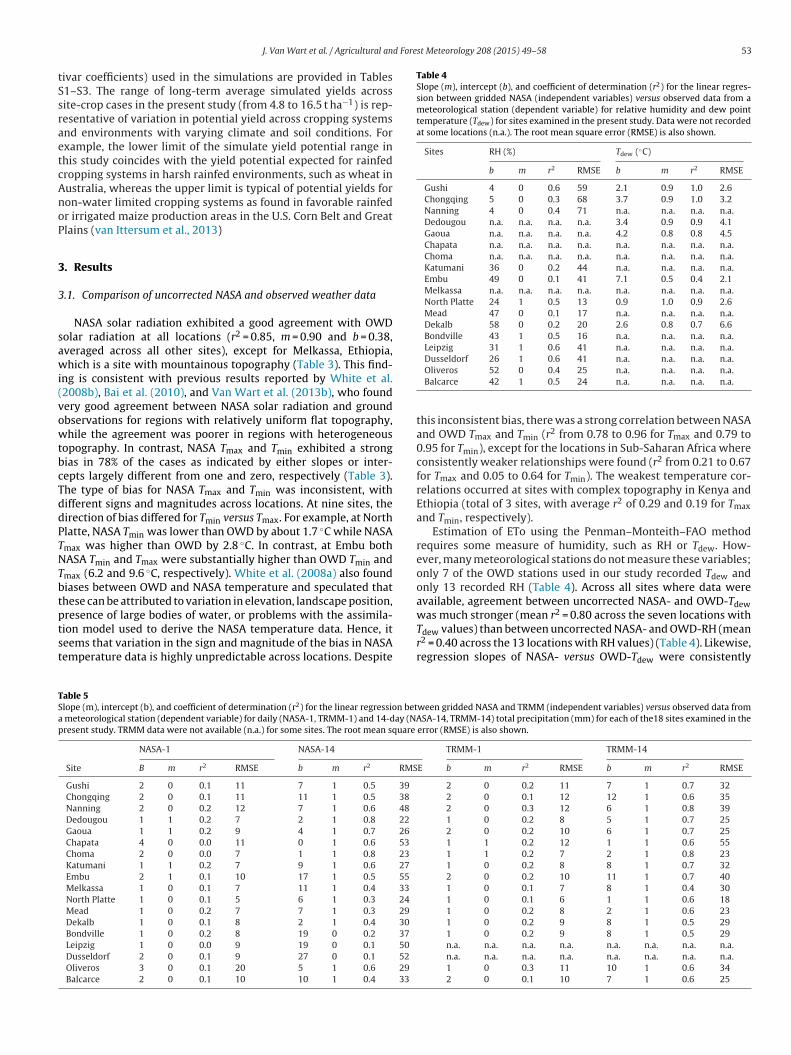
d Forest Meteorology 208 (2015) 49–58 53

tSsraetcAnoP

3

3

sawi(vowtbcTddPTNTbtptst

Table 4Slope (m), intercept (b), and coefficient of determination (r2) for the linear regres-sion between gridded NASA (independent variables) versus observed data from ameteorological station (dependent variable) for relative humidity and dew pointtemperature (Tdew) for sites examined in the present study. Data were not recordedat some locations (n.a.). The root mean square error (RMSE) is also shown.

Sites RH (%) Tdew (◦C)

b m r2 RMSE b m r2 RMSE

Gushi 4 0 0.6 59 2.1 0.9 1.0 2.6Chongqing 5 0 0.3 68 3.7 0.9 1.0 3.2Nanning 4 0 0.4 71 n.a. n.a. n.a. n.a.Dedougou n.a. n.a. n.a. n.a. 3.4 0.9 0.9 4.1Gaoua n.a. n.a. n.a. n.a. 4.2 0.8 0.8 4.5Chapata n.a. n.a. n.a. n.a. n.a. n.a. n.a. n.a.Choma n.a. n.a. n.a. n.a. n.a. n.a. n.a. n.a.Katumani 36 0 0.2 44 n.a. n.a. n.a. n.a.Embu 49 0 0.1 41 7.1 0.5 0.4 2.1Melkassa n.a. n.a. n.a. n.a. n.a. n.a. n.a. n.a.North Platte 24 1 0.5 13 0.9 1.0 0.9 2.6Mead 47 0 0.1 17 n.a. n.a. n.a. n.a.Dekalb 58 0 0.2 20 2.6 0.8 0.7 6.6Bondville 43 1 0.5 16 n.a. n.a. n.a. n.a.Leipzig 31 1 0.6 41 n.a. n.a. n.a. n.a.Dusseldorf 26 1 0.6 41 n.a. n.a. n.a. n.a.

TSap

J. Van Wart et al. / Agricultural an

ivar coefficients) used in the simulations are provided in Tables1–S3. The range of long-term average simulated yields acrossite-crop cases in the present study (from 4.8 to 16.5 t ha−1) is rep-esentative of variation in potential yield across cropping systemsnd environments with varying climate and soil conditions. Forxample, the lower limit of the simulate yield potential range inhis study coincides with the yield potential expected for rainfedropping systems in harsh rainfed environments, such as wheat inustralia, whereas the upper limit is typical of potential yields foron-water limited cropping systems as found in favorable rainfedr irrigated maize production areas in the U.S. Corn Belt and Greatlains (van Ittersum et al., 2013)

. Results

.1. Comparison of uncorrected NASA and observed weather data

NASA solar radiation exhibited a good agreement with OWDolar radiation at all locations (r2 = 0.85, m = 0.90 and b = 0.38,veraged across all other sites), except for Melkassa, Ethiopia,hich is a site with mountainous topography (Table 3). This find-

ng is consistent with previous results reported by White et al.2008b), Bai et al. (2010), and Van Wart et al. (2013b), who foundery good agreement between NASA solar radiation and groundbservations for regions with relatively uniform flat topography,hile the agreement was poorer in regions with heterogeneous

opography. In contrast, NASA Tmax and Tmin exhibited a strongias in 78% of the cases as indicated by either slopes or inter-epts largely different from one and zero, respectively (Table 3).he type of bias for NASA Tmax and Tmin was inconsistent, withifferent signs and magnitudes across locations. At nine sites, theirection of bias differed for Tmin versus Tmax. For example, at Northlatte, NASA Tmin was lower than OWD by about 1.7 ◦C while NASAmax was higher than OWD by 2.8 ◦C. In contrast, at Embu bothASA Tmin and Tmax were substantially higher than OWD Tmin and

max (6.2 and 9.6 ◦C, respectively). White et al. (2008a) also foundiases between OWD and NASA temperature and speculated thathese can be attributed to variation in elevation, landscape position,

resence of large bodies of water, or problems with the assimila-ion model used to derive the NASA temperature data. Hence, iteems that variation in the sign and magnitude of the bias in NASAemperature data is highly unpredictable across locations. Despite

able 5lope (m), intercept (b), and coefficient of determination (r2) for the linear regression bet

meteorological station (dependent variable) for daily (NASA-1, TRMM-1) and 14-day (NAresent study. TRMM data were not available (n.a.) for some sites. The root mean square

NASA-1 NASA-14

Site B m r2 RMSE b m r2 RMS

Gushi 2 0 0.1 11 7 1 0.5 39

Chongqing 2 0 0.1 11 11 1 0.5 38

Nanning 2 0 0.2 12 7 1 0.6 48

Dedougou 1 1 0.2 7 2 1 0.8 22

Gaoua 1 1 0.2 9 4 1 0.7 26

Chapata 4 0 0.0 11 0 1 0.6 53

Choma 2 0 0.0 7 1 1 0.8 23

Katumani 1 1 0.2 7 9 1 0.6 27

Embu 2 1 0.1 10 17 1 0.5 55

Melkassa 1 0 0.1 7 11 1 0.4 33

North Platte 1 0 0.1 5 6 1 0.3 24

Mead 1 0 0.2 7 7 1 0.3 29

Dekalb 1 0 0.1 8 2 1 0.4 30

Bondville 1 0 0.2 8 19 0 0.2 37

Leipzig 1 0 0.0 9 19 0 0.1 50

Dusseldorf 2 0 0.1 9 27 0 0.1 52

Oliveros 3 0 0.1 20 5 1 0.6 29

Balcarce 2 0 0.1 10 10 1 0.4 33

Oliveros 52 0 0.4 25 n.a. n.a. n.a. n.a.Balcarce 42 1 0.5 24 n.a. n.a. n.a. n.a.

this inconsistent bias, there was a strong correlation between NASAand OWD Tmax and Tmin (r2 from 0.78 to 0.96 for Tmax and 0.79 to0.95 for Tmin), except for the locations in Sub-Saharan Africa whereconsistently weaker relationships were found (r2 from 0.21 to 0.67for Tmax and 0.05 to 0.64 for Tmin). The weakest temperature cor-relations occurred at sites with complex topography in Kenya andEthiopia (total of 3 sites, with average r2 of 0.29 and 0.19 for Tmax

and Tmin, respectively).Estimation of ETo using the Penman–Monteith–FAO method

requires some measure of humidity, such as RH or Tdew. How-ever, many meteorological stations do not measure these variables;only 7 of the OWD stations used in our study recorded Tdew andonly 13 recorded RH (Table 4). Across all sites where data wereavailable, agreement between uncorrected NASA- and OWD-Tdew

was much stronger (mean r2 = 0.80 across the seven locations withTdew values) than between uncorrected NASA- and OWD-RH (meanr2 = 0.40 across the 13 locations with RH values) (Table 4). Likewise,regression slopes of NASA- versus OWD-Tdew were consistently

ween gridded NASA and TRMM (independent variables) versus observed data fromSA-14, TRMM-14) total precipitation (mm) for each of the18 sites examined in the

error (RMSE) is also shown.

TRMM-1 TRMM-14

E b m r2 RMSE b m r2 RMSE

2 0 0.2 11 7 1 0.7 322 0 0.1 12 12 1 0.6 352 0 0.3 12 6 1 0.8 391 0 0.2 8 5 1 0.7 252 0 0.2 10 6 1 0.7 251 1 0.2 12 1 1 0.6 551 1 0.2 7 2 1 0.8 231 0 0.2 8 8 1 0.7 322 0 0.2 10 11 1 0.7 401 0 0.1 7 8 1 0.4 301 0 0.1 6 1 1 0.6 181 0 0.2 8 2 1 0.6 231 0 0.2 9 8 1 0.5 291 0 0.2 9 8 1 0.5 29n.a. n.a. n.a. n.a. n.a. n.a. n.a. n.a.n.a. n.a. n.a. n.a. n.a. n.a. n.a. n.a.1 0 0.3 11 10 1 0.6 342 0 0.1 10 7 1 0.6 25

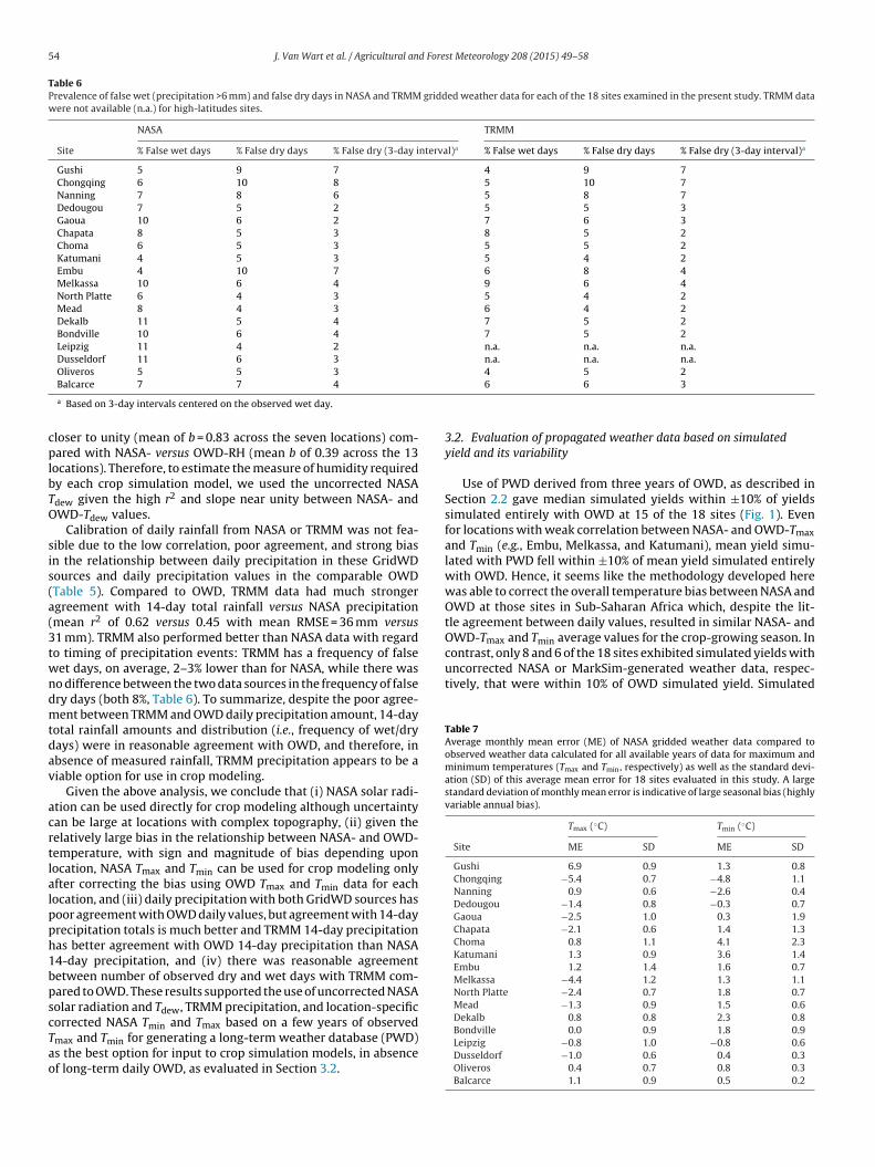
54 J. Van Wart et al. / Agricultural and Forest Meteorology 208 (2015) 49–58

Table 6Prevalence of false wet (precipitation >6 mm) and false dry days in NASA and TRMM gridded weather data for each of the 18 sites examined in the present study. TRMM datawere not available (n.a.) for high-latitudes sites.

NASA TRMM

Site % False wet days % False dry days % False dry (3-day interval)a % False wet days % False dry days % False dry (3-day interval)a

Gushi 5 9 7 4 9 7Chongqing 6 10 8 5 10 7Nanning 7 8 6 5 8 7Dedougou 7 5 2 5 5 3Gaoua 10 6 2 7 6 3Chapata 8 5 3 8 5 2Choma 6 5 3 5 5 2Katumani 4 5 3 5 4 2Embu 4 10 7 6 8 4Melkassa 10 6 4 9 6 4North Platte 6 4 3 5 4 2Mead 8 4 3 6 4 2Dekalb 11 5 4 7 5 2Bondville 10 6 4 7 5 2Leipzig 11 4 2 n.a. n.a. n.a.Dusseldorf 11 6 3 n.a. n.a. n.a.Oliveros 5 5 3 4 5 2

cplbTO

sis(a(3twndmtdav

acrtlalpph1bpscTao

contrast, only 8 and 6 of the 18 sites exhibited simulated yields withuncorrected NASA or MarkSim-generated weather data, respec-tively, that were within 10% of OWD simulated yield. Simulated

Table 7Average monthly mean error (ME) of NASA gridded weather data compared toobserved weather data calculated for all available years of data for maximum andminimum temperatures (Tmax and Tmin, respectively) as well as the standard devi-ation (SD) of this average mean error for 18 sites evaluated in this study. A largestandard deviation of monthly mean error is indicative of large seasonal bias (highlyvariable annual bias).

Tmax (◦C) Tmin (◦C)

Site ME SD ME SD

Gushi 6.9 0.9 1.3 0.8Chongqing −5.4 0.7 −4.8 1.1Nanning 0.9 0.6 −2.6 0.4Dedougou −1.4 0.8 −0.3 0.7Gaoua −2.5 1.0 0.3 1.9Chapata −2.1 0.6 1.4 1.3Choma 0.8 1.1 4.1 2.3Katumani 1.3 0.9 3.6 1.4Embu 1.2 1.4 1.6 0.7Melkassa −4.4 1.2 1.3 1.1North Platte −2.4 0.7 1.8 0.7Mead −1.3 0.9 1.5 0.6Dekalb 0.8 0.8 2.3 0.8Bondville 0.0 0.9 1.8 0.9

Balcarce 7 7 4

a Based on 3-day intervals centered on the observed wet day.

loser to unity (mean of b = 0.83 across the seven locations) com-ared with NASA- versus OWD-RH (mean b of 0.39 across the 13

ocations). Therefore, to estimate the measure of humidity requiredy each crop simulation model, we used the uncorrected NASAdew given the high r2 and slope near unity between NASA- andWD-Tdew values.

Calibration of daily rainfall from NASA or TRMM was not fea-ible due to the low correlation, poor agreement, and strong biasn the relationship between daily precipitation in these GridWDources and daily precipitation values in the comparable OWDTable 5). Compared to OWD, TRMM data had much strongergreement with 14-day total rainfall versus NASA precipitationmean r2 of 0.62 versus 0.45 with mean RMSE = 36 mm versus1 mm). TRMM also performed better than NASA data with regardo timing of precipitation events: TRMM has a frequency of falseet days, on average, 2–3% lower than for NASA, while there was

o difference between the two data sources in the frequency of falsery days (both 8%, Table 6). To summarize, despite the poor agree-ent between TRMM and OWD daily precipitation amount, 14-day

otal rainfall amounts and distribution (i.e., frequency of wet/dryays) were in reasonable agreement with OWD, and therefore, inbsence of measured rainfall, TRMM precipitation appears to be aiable option for use in crop modeling.

Given the above analysis, we conclude that (i) NASA solar radi-tion can be used directly for crop modeling although uncertaintyan be large at locations with complex topography, (ii) given theelatively large bias in the relationship between NASA- and OWD-emperature, with sign and magnitude of bias depending uponocation, NASA Tmax and Tmin can be used for crop modeling onlyfter correcting the bias using OWD Tmax and Tmin data for eachocation, and (iii) daily precipitation with both GridWD sources hasoor agreement with OWD daily values, but agreement with 14-dayrecipitation totals is much better and TRMM 14-day precipitationas better agreement with OWD 14-day precipitation than NASA4-day precipitation, and (iv) there was reasonable agreementetween number of observed dry and wet days with TRMM com-ared to OWD. These results supported the use of uncorrected NASAolar radiation and Tdew, TRMM precipitation, and location-specificorrected NASA Tmin and Tmax based on a few years of observed

max and Tmin for generating a long-term weather database (PWD)s the best option for input to crop simulation models, in absencef long-term daily OWD, as evaluated in Section 3.2.

6 6 3

3.2. Evaluation of propagated weather data based on simulatedyield and its variability

Use of PWD derived from three years of OWD, as described inSection 2.2 gave median simulated yields within ±10% of yieldssimulated entirely with OWD at 15 of the 18 sites (Fig. 1). Evenfor locations with weak correlation between NASA- and OWD-Tmax

and Tmin (e.g., Embu, Melkassa, and Katumani), mean yield simu-lated with PWD fell within ±10% of mean yield simulated entirelywith OWD. Hence, it seems like the methodology developed herewas able to correct the overall temperature bias between NASA andOWD at those sites in Sub-Saharan Africa which, despite the lit-tle agreement between daily values, resulted in similar NASA- andOWD-Tmax and Tmin average values for the crop-growing season. In

Leipzig −0.8 1.0 −0.8 0.6Dusseldorf −1.0 0.6 0.4 0.3Oliveros 0.4 0.7 0.8 0.3Balcarce 1.1 0.9 0.5 0.2

J. Van Wart et al. / Agricultural and Forest Meteorology 208 (2015) 49–58 55

7.28.94.86.36.69.0

12.715.716.59.0

10.56.56.17.46.06.36.9

10.0

OWD-Yld(t ha-1)

Deviation from long-t erm ave rage simulated yields using OWD (%)

-60 % -40 % -20 % 0% 20 % 40 % 60 %

Chapata (M)Cho ma (M)

Dedou gou (M)Embu (M)

Gaou a (M)Katumani (M )Melkassa (M)Balca rce (M)Olive ros (M)

Bondville (M)DeKalb (M )

Mead (M)North Platt e (M )

Gushi (R)ChongQing (R)

Nann ing (R)Leipzig (W)

Dusse ldo rf (W)

Fig. 1. Distribution of long-term average yields simulated with all possible subsets of propagated weather data (PWD, boxplots) derived from calibration with 3-year ofobserved weather data (OWD) and their deviation from long-term average yield simulated entirely with OWD for maize (M), rice (R), or wheat (W) at 18 locations. Yieldssimulated with uncorrected NASA weather data (red triangles) and MarkSim weather data (yellow squares) are also shown. Boxplots display percent differences betweenlong-term average yields simulated entirely with OWD and yields simulated with PWD calibrated with all possible subsets of 3-year OWD series. Lower and upper boundariesfor each box are the 25th and 75th percentiles. The line inside each box indicates the median. Whiskers (error bars) above and below the box indicate the 90th and 10thpercentiles. Deviation of ±10% is shown as shaded background. Long-term average yields based on OWD are displayed in a table along the Y axis (OWD-Yld). MarkSim basedyields at Gushi were too high to be shown (94% higher than OWD-based simulation). (For interpretation of the references to color in this figure legend, the reader is referredto the web version of this article.)

Fig. 2. Distribution of long-term average simulated yields using propagated weather data (PWD) when 3–5 and 10-year subsets of observed data (OWD) are used to correctNASA maximum and minimum temperatures (Tmax) and (Tmin) based on an annual calibration (left panels for both Chongquin and Choma locations) versus simulations inwhich PWD for Chongqing included a site-specific correction for solar radiation (SR, upper right panel) or a seasonally calibrated Tmin and Tmax for Choma (lower right panel).The box plots display the median, 10th, 25th, 75th, and 90th percentiles as vertical boxes with error bars. For reference, long-term average yields simulated using OWD (blueline) and ±10% of long term average yields simulated using OWD (dashed blue lines) are overlaid across the chart. (For interpretation of the references to color in this figurelegend, the reader is referred to the web version of this article.)

56 J. Van Wart et al. / Agricultural and Forest Meteorology 208 (2015) 49–58

Difference from CV of simulations made us ing OWD (%)

-30 % -20 % -10% 0% 10 % 20 % 30 %

Chapa ta (M)Cho ma (M)

Dedougou (M)Embu (M)

Gaou a (M)Katumani (M)Melkassa (M)Balca rce (M)Oliveros (M)

Bondville (M)DeKalb (M)

Mead (M)North Platte (M)

Gushi (R)ChongQing (R)

Nann ing (R)Leipzig (W)

Dusse ldo rf (W) 5%17%3%4%3%7%6%

22%24%17%13%18%17%16%21%13%9%6%

OWD-CV(t ha-1)

Fig. 3. Distribution of inter-annual coefficient of variation (CV) in yields simulated with all possible subsets of propagated weather data (PWD, boxplots) derived fromcalibration with 3-year of observed weather data (OWD) and deviation of these CVs from long-term average CV from simulations based entirely on OWD for maize (M), rice(R), or wheat (W) at 18 locations. CV of simulated yield with uncorrected NASA weather data (red triangles) and MarkSim weather data (yellow squares) are also shown. Boxplots display difference between CV of OWD-based simulations and CVs of simulated yields based on PWD calibrated with all possible 3-year subsets of OWD. Lower andupper boundaries for each box are the 25th and 75th percentiles. The line inside each box indicates the median. Whiskers (error bars) above and below the box indicate the90th and 10th percentiles. Differences of ±5% are shown as shaded background. CV of simulated yields based on OWD are displayed in a table along the Y axis (OWD-CV).M basedr

lwrSMtsaoo

wipo(TberisWywtHsc

sdF

arkSim based yields at Nanning are too high to be shown (94% larger than OWD-eader is referred to the web version of this article.)

ong-term average yields using uncorrected NASA data combinedith TRMM precipitation were very similar to those with uncor-

ected NASA weather data that included NASA precipitation (Fig.1). The bias between yields simulated with uncorrected NASA orarkSim weather data and OWD-simulated yields was inconsis-

ent across locations. Use of uncorrected NASA data led to meanimulated yields outside the ±10% OWD-yield band in 33% (above)nd 22% (below) of the cases (Fig. 1). MarkSim-simulated yields fellutside the ±10% OWD-yield band in 22% (above) and 44% (below)f the cases.

Results for two sites at which a majority of yields simulatedith PWD fell outside the ±10% OWD-yield band were further

nvestigated to identify the cause of the discrepancy. For exam-le, regardless of how many years were used in the calibrationf NASA Tmax and Tmin, simulated yields with PWD at ChongQingChina) were about 34% higher than OWD-simulated yields (Fig. 2).he over-estimation was caused by the difference in solar radiationetween NASA and OWD, which, in turn was associated with het-rogeneous topography at this site. Similar discrepancies in solaradiation have been found at locations with complex topographyn previous studies that evaluated use of NASA weather data forimulation of crop yields (Bai et al., 2010; White et al., 2008b; Van

art et al., 2013b). At Choma, a site with mean PWD-simulatedields 13% higher than OWD yields, the higher simulated yieldsith PWD were associated with seasonal differences in the magni-

ude of the bias between NASA and OWD Tmax and Tmin (Table 7).ence, calibration of NASA daily temperatures based on regres-

ion with the observed short-term weather data did not provide aonsistent correction for propagated Tmax and Tmin for this site.

PWD-simulated yields at these two locations could be sub-

tantially improved, however, by addressing the location-specificiscrepancies between NASA and OWD weather databases (Fig. 2).or ChongQing, calibrating NASA solar radiation, using the same

simulation). (For interpretation of the references to color in this figure legend, the

calibration method as used to correct NASA Tmin and Tmax, resultedin PWD-simulated yields in close agreement with OWD-simulatedyields. Similarly, PWD-simulated yields at Choma were much moreconsistent with OWD yields when NASA Tmin and Tmax were cal-ibrated separately for four subsets of three consecutive months,which accounts for the seasonal difference in the bias betweenNASA and OWD Tmin and Tmax. Thus, for both sites, a location-specific calibration of the biased weather variable, solar radiationat ChongQing and temperature at Choma, resulted in mean PWD-simulated yield and 75% of the simulated yield distribution withinthe ±10% OWD-yield band.

Coefficient of variation of PWD-simulated yields was remark-ably similar to the degree of variation observed in OWD yields. In16 of 18 sites, the distribution of CVs in PWD yields were within±5% of the CV calculated for OWD yields (Fig. 3). In contrast, yieldssimulated with NASA- or MarkSim weather data had CVs withinthe ±5% CV band of OWD yields in 15 and 9 sites, respectively.While simulated yields using PWD had similar long-term yieldsand CVs compared with yields simulated entirely with OWD, simu-lation of yields for individual years was more uncertain across sitesand years when compared to simulated yields with OWD for thesame year (Fig. S2). Therefore, PWD generated using the methoddescribed in this paper is considerably more robust at simulatinglong-term average yields than the yield of a single year.

4. Discussion

GridWD or GenWD are typically used to simulate yields in stud-ies that evaluate crop performance at locations without long-term

OWD (Table 1). At issue is the accuracy and precision of such esti-mates and whether it is possible to improve the methods usedto derive long-term GenWD. To that end, we present an alterna-tive method to propagate long-term daily weather data based on

d Fore

spaUa2otadmg

octtwsrtHccasgalE(h2ie

araGspuhPtucts

A

tNCStCtCYsO

J. Van Wart et al. / Agricultural an

olar radiation and Tdew from the NASA gridded weather database,recipitation from TRMM rainfall, and calibration of NASA Tmax

nd Tmin using three years of observed data at a given location.nlike some of the more sophisticated GenWD, which may require

decade or more of OWD for calibration (Baigorria and Jones,010), the new approach developed herein requires only 3 yearsf observed temperature data and thus may be useful for loca-ions with short-term weather datasets (e.g., crop breeding trials orgronomy experiment stations in developing countries). Whereasaily temperature data are often measured at such locations, instru-entation to measure solar radiation is rare and there can be large

aps of missing data in recorded daily rainfall.Simulated yields of the major cereals across a wide range

f environments using PWD, following the described protocol,learly outperformed NASA-GridWD or MarkSim-GenWD, relativeo agreement with simulated yields using OWD. comparable tohose simulated using OWD. Overall, PWD-based simulations wereithin ±10% of OWD-based long-term average yields at 78% of all

ites versus only 44% and 33% of the sites using GWS and GenWD,espectively, regardless of whether 3, 4, 5, or 10 years of tempera-ure data were used for location-specific temperature calibration.ence, 3 years of observed temperature data appear to be suffi-

ient for deriving a robust PWD set. We conclude, therefore, thatreation of PWD, as performed in this study, provides a reliablend superior alternative for crop simulation to use of GridWDuch as NASA (evaluated in this study) or the MarkSim weatherenerator (GenWD) for locations where long-term OWD are notvailable. It is also notable that the PWD as described herein areikely to outperform other GridWD such as the National Center fornvironmental Prediction and Department of Energy’s reanalysis IINCEP/DOE, Kanamitsu et al., 2002) or the Climate Research Unit’sigh-resolution gridded dataset time series 3.1 (CRU, New et al.,002) based on previous comparisons with NASA and OWD data

n simulating long-term crop yields and their variability (Van Wartt al., 2013b).

While PWD-based simulations captured inter-annual variationnd long-term average yields quite well, they are sometimes noteliable for accurate simulation of yield in a specific year. PWDre also subjected to bias in those variables taken directly fromridWD without calibration such as TRMM precipitation and NASA

olar radiation and Tdew. Hence, whenever these variables haveoor agreement with ground observations, there will be largencertainty in the PWD-simulated yields. Even in these cases,owever, results of our study suggest that simulations based onWD are in better agreement with simulated yields with OWDhan simulations based on the other sources of weather data eval-ated in this study. For some locations, the reliability of PWDan be further improved by using seasonal calibration of GridWDemperature rather than an annual calibration as used in thistudy.

cknowledgements

Support for various aspects of this research was provided byhe Robert Daugherty Water for Food Institute at the University ofebraska-Lincoln, the Bill and Melinda Gates Foundation, and theGIAR research program on Climate Change, Agriculture and Foodecurity (CCAFS). We thank Drs. Shaobing Ping (Huazhong Agricul-ure University, China), Jingshun Bai (China Agricultural University,hina), and Christian K. Kersebaum (Leibniz Centre for Agricul-ural Landscape Research, Germany) for proving weather data from

hina and Germany and agronomists contributing to the Globalield Gap Atlas for providing weather and management data foreveral countries in Sub-Saharan Africa, including Dr. Korodjoumauattara (Institut de l’Environnement et de Recherches agricoles,

st Meteorology 208 (2015) 49–58 57

Burkina Faso), Dr. Ochieng Adimo (Jomo Kenyatta University ofAgriculture and Technology, Kenya), and Dr. Regis Chikowo (Uni-versity of Zimbabwe).

Appendix A. Supplementary data

Supplementary data associated with this article can be found,in the online version, at http://dx.doi.org/10.1016/j.agrformet.2015.02.020.

References

Abraha, M.G., Savage, M.J., 2006. Potential impacts of climate change on grain yieldof maize for the midlands of KwaZulu-Natal, South Africa. Agric. Ecosyst.Environ. 115, 150–160.

Allen, R.G., Pereira, L.S., Raes, D., Smith, M., 1998. Crop Evapotranspiration:Guidelines for Computing Crop Water Requirements, FAO Irrigation andDrainage Paper 56. FAO, Rome, Italy.

Arndt, C., Farmer, W., Strzepek, K., Thurlow, J., 2012. Climate change, agricultureand food security in Tanzania. Rev. Dev. Econ. 16, 378–393.

Bagley, J.E., Desai, A.R., Dirmeyer, P.A., Foley, J.A., 2012. Effects of land cover changeon moisture availability and potential crop yield in the world’s breadbaskets.Envir. Res. Lett. 7, 1–9.

Bai, J., Chen, X., Dobermann, A., Yang, H., Cassman, K.G., Zhang, F., 2010. Evaluationof NASA satellite- and model-derived weather data for simulation of maizeyield potential in China. Agron. J. 102, 9–16.

Baigorria, G.A., Jones, J., 2010. GIST, a stochastic model for generating spatially andtemporally correlated daily rainfall data. J. Clim. 23, 5990–6008.

Baron, C., Sultan, B., Balme, M., Sarr, B., Traore, S., Lebel, T., Janicot, S., Dingkuhn, M.,2005. From GCM grid cell to agricultural plot: same scale issues affectingmodelling of climate impact. Philos. Trans. R. Soc. London Ser. B 360,2095–2108.

Battisti, D.S., Naylor, R.L., 2009. Historical warnings of future food insecurity withunprecedented seasonal heat. Science 323, 240–244.

Bondeau, A., Smith, P.C., Zaehle, S., Schaphoff, S., Lucht, W., Cramer, W., Gerten, D.,Lotze-Campen, H., Müller, C., Reichstein, M., Smith, B., 2007. Modelling the roleof agriculture for the 20th century global terrestrial carbon balance. GlobalChange Biol. 13, 679–706.

Boote, K.J., Jones, J.W., Pickering, N.B., 1996. Potential uses and limitations of cropmodels. Agron. J. 88, 704–716.

Bouman, B.A.M., Kropff, M.J., Tuong, T.P., Wopereis, M.C.S., Ten Berge, H.F.M., vanLaar, H.H., 2001. Oryza2000: Modeling Lowland Rice. International RiceResearch Institute, Los Banos, Philippines.

Bouman, B.A.M., van Laar, H.H., 2006. Description and evaluation of the rice growthmodel ORYZA2000 under nitrogen-limited conditions. Agric. Syst. 87,249–273.

Chandler, W.S., Whitlock, C.H., Stackhouse Jr., P.W., 2004. NASA climatological datafor renewable energy assessment. J. Solar Energy Eng. 126, 945–949.

Claessens, L., Antle, J.M., Stoorvogel, J.J., Valdivia, R.O., Thornton, P.K., Herrero, M.,2012. A method for evaluating climate change adaptation strategies forsmall-scale farmers using survey: experimental and modeled data. Agric. Syst.111, 85–95.

Fischer, G., van Velthuizen, H., Shah, M., Nachtergaele, F.O., 2002. GlobalAgroecological Assessment for Agriculture in the 21st Century: Methodologyand Results. IIASA Research Report RR-02-02, Laxenburg, Austria.

Folberth, C., Gaiser, T., Abbaspour, K.C., Schulin, R., Yang, H., 2012. Regionalizationof a large-scale crop growth model for Sub-Saharan Africa Model setup,evaluation, and estimation of maize yields. Agric. Ecosyst. Environ. 151, 21–33.

Folberth, C., Yang, H., Gaiser, T., Abbaspour, K.C., Schulin, R., 2013. Modeling maizeyield responses to improvement in nutrient, water and cultivar inputs inSub-Saharan Africa. Agric. Syst. 119, 22–34.

Foley, J.A., Defries, R., Asner, G.P., Barford, C., Bonan, G., Carpenter, S.R., Chapin, F.S.,Coe, M.C., Daily, G.C., Gibbs, H.K., Helkowski, J.H., Holloway, T., Howard, E.A.,Kucharik, C.J., Monfreda, C., Patz, J.A., Prentice, I.C., Ramankutty, N., Synder,P.K., 2005. Global consequences of land use. Science 309, 570–574.

Ghaffari, A., Cook, H.F., Lee, H.C., 2001. Simulating winter wheat yields undertemperate conditions: exploring different management scenarios. Eur. J.Agron. 15, 231–240.

Grassini, P., Yang, H.S., Cassman, K.G., 2009. Limits to maize productivity inWestern Corn-Belt: a simulation analysis for fully irrigated and rainfedconditions. Agric. For. Meteorol. 149, 1254–1265.

Grassini, P., Van Bussel, L.G.J., Van Wart, J., Wolf, J., Claessens, L., Yang, H.,Boogaard, H., de Groot, H., Van Ittersum, M.K., Cassman, K.G., 2015. How goodis good enough? Data requirements for reliable crop yield simulations andyield-gap analysis. Field Crops Res. 177, 49–63.

Hammer, G.L., Kropff, M.J., Sinclair, T.R., Porter, J.R., 2002. Future contributions of

crop modelling-from heuristics and supporting decision making tounderstanding genetic regulation and aiding crop improvement. Eur. J. Agron.18, 15–31.

Hansen, J.W., Mavromatis, T., 2001. Correcting low-frequency variability bias instochastic weather generators. Agric. For. Meteorol. 109, 297–310.

5 d Fore

H

H

J

J

J

K

K

K

L

L

L

L

L

L

M

M

M

N

N

satellite-based, modeled-derived daily solar radiation data for the continentalUnited States. Agric. For. Meteorol. 148, 1574–1584.

Yang, H.S., Dobermann, A., Lindquist, J.L., Walters, D.T., Arkebauer, T.J., Cassman,

8 J. Van Wart et al. / Agricultural an

ubbard, K.G., You, J., 2005. Sensitivity analysis of quality assurance using spatialregression approach—a case study of maximum/minimum air temperature. J.Atmos. Oceanic Technol. 22, 1520–1530.

utchinson, M.F., 1987. Methods of generation of weather sequences. In: Bunting,A.H. (Ed.), Agricultural Environments: Characterization, Classification andMapping. CAB International, Cambridge.

ones, P.G., Thornton, P.K., 2003. The potential impacts of climate change on maizeproduction in Africa and Latin America in 2055. Global Environ. Change 13,51–59.

ones, P.G., Thornton, P.K., 2000. Marksim: Software to generate daily weather datafor Latin America and Africa. Agron. J. 92, 445–453.

ones, P.G., Thornton, P.K., 2013. Generating downscaled weather data from a suiteof climate models for agricultural modelling applications. Agric. Syst. 114,1–5.

anamitsu, M., Ebisuzaki, W., Woolen, J., Yang, S., Hnilo, J.J., Fiorino, M., Potter, G.L.,2002. NCEP–DOE AMIP-II reanalysis (R-2). Bull. Am. Meteorol. Soc. 83,1631–1643.

ummerow, C., Simpson, J., Thiele, O., Barnes, W., Chang, A.T.C., Stocker, E., Adler,R.F., Hou, A., Kakar, R., Wentz, F., Ashcroft, P., Kozu, T., Hong, Y., Okamoto, K.,Iguchi, T., Kuroiwa, H., Im, E., Haddad, Z., Huffman, G., Ferrier, B., Olson, W.S.,Zipser, E., Smith, E.A., Wilheit, T.T., North, G., Krishnamurti, T., Nakamura, K.,2000. The status of the Tropical Rainfall Measuring Mission (TRMM) after twoyears in orbit. J. Appl. Meteorol. 39, 1965–1982.

ysely, J., Dubrovsky, M., 2005. Simulation of extreme temperature events by astochastic weather generator: effects of interdiurnal and interannualvariability reproduction. Int. J. Clim. 25, 251–269.

aux, P., Jäckela, G., Tingem, R.M., Kunstmann, H., 2010. Impact of climate changeon agricultural productivity under rainfed conditions in Cameroon – a methodto improve attainable crop yields by planting date adaptations. Agric. For.Meteorol. 150, 1258–1271.

i, K.Y., Coe, M.T., Ramankutty, N., 2005. Investigation of hydrological variability inWest Africa using land surface models. J. Clim. 18, 3173–3188.

icker, R., Johnston, M., Foley, J.A., Barford, C., Kucharik, C.J., Monfreda, C.,Ramankutty, N., 2010. Mind the gap: how do climate and agriculturalmanagement explain the ‘yield gap’ of croplands around the world? Glob. Ecol.Biogeogr. 19, 769–782.

obell, D., 2007. Changes in diurnal temperature range and national cereal yields.Agric. For. Meteorol. 145, 229–238.

obell, D.B., Asner, G.P., 2003. Climate and management contributions to recenttrends in U.S. agricultural yields. Science 299, 1032.

obell, D.B., Burke, M.B., Tebaldi, C., Mastrandrea, M.D., Falcon, W.P., Naylor, R.L.,2008. Prioritizing climate change adaptation needs for food security in 2030.Science 319, 607–610.

ahmood, R., Hubbard, K.G., 2002. Effect of time of temperature observations andestimation on daily solar radiation for the Northern Great Plains, USA. Agron. J.94, 723–733.

avromatis, T., Hansen, J.W., 2001. Interannual variability characteristics andsimulated crop response of four stochastic weather generators. Agric. For.Meteorol. 109, 283–296.

earns, L.O., Easterling, W., Hays, C.J., Marx, D., 2001. Comparison of agriculturalimpacts of climate change calculated from high and low resolution climatechange scenarios: part I. The uncertainty due to spatial scale. Clim. Change 51,131–172.

ASA, 2012. NASA-Agroclimatology methodology. Available at:http://power.larc.nasa.gov/common/AgroclimatologyMethodology/Agro1d0

Methodology Content.html (accessed 09.13.).

ational Climate Data Center, 2014. Global surface summary of the day- Climatedata online. Available at:http://www7ncdc.noaa.gov/CDO/cdoselect.cmd?datasetabbv=GSOD&countryabbv=&georegionabbv= (accessed 01.14.).

st Meteorology 208 (2015) 49–58

Nelson, G.C., Rosegrant, M.W., Palazzo, A., Gran, I., Ingersoll, C., Robertson, R.,Tokgoz, S., Zhu, T., Sulser, T.B., Ringler, C., Msangi, S., You, L., 2010. FoodSecurity, Farming and Climate Change to 2050. International Food PolicyResearch Institute, Washington, DC.

Nemani, R.R., Keeling, C.D., Hashimoto, H., Jolly, W.M., Piper, S.C., Tucker, C.J.,Myneni, R.B., Running, S.W., 2003. Climate-driven increases in globalterrestrial net primary production from 1982 to 1999. Science 300, 1560–1563.

New, M., Lister, D., Hulme, M., Makin, I., 2002. A high-resolution data set of surfaceclimate over global land areas. Clim. Res. 21, 1–25.

Ritchie, J.T., Godwin, D.C., Otter-Nacke, S., 1988. CERES-Wheat. University of TexasPress, Austin, TX.

Rosenzweig, C., Jones, J.W., Hatfield, J.L., Ruane, A.C., Boote, K.J., Thorburn, P., Antle,J.M., Nelson, G.C., Porter, C., Janssen, S., Asseng, S., Basso, B., Ewert, F., Wallach,D., Baigorria, G., Winter, J.M., 2013. The agricultural model intercomparisonand improvement project (AgMIP): protocols and pilot studies. Agric. For.Meteorol. 170, 166–182.

Rowhani, P., Lobell, D.B., Linderman, M., Ramankutty, N., 2011. Climate variabilityand crop production in Tanzania. Agric. For. Meteorol. 151, 449–460.

Sadras, V.O., 2003. Influence of size of rainfall events on water-driven processes. I.Water budget of wheat crops in south-eastern Australia. Aust. J. Agric. Res. 54,341–351.

Schuol, J., Abbaspour, K.C., Srinivasan, R., Yang, H., 2008. Estimation of freshwateravailability in the West African sub-continent using the SWAT hydrologicmodel. J. Hydrol. 352, 30–49.

Semenov, M.A., Porter, J.R., 1995. Climatic variability and the modeling of cropyields. Agric. For. Meteorol. 73, 265–283.

Semenov, M., 2008. Simulation of extreme weather events by a stochastic weathergenerator. Clim. Res. 35, 203–212.

Stéphenne, N., Lambin, E.F., 2001. A dynamic simulation model of land-usechanges in Sudano-sahelian countries of Africa (SALU). Agric. Ecosyst. Environ.85, 145–161.

Thornton, P.K., Jones, P.G., Alagarswamy, G., Andresen, J., 2009. Spatial variation ofcrop yield response to climate change in East Africa. Global Environ. Change19, 54–65.

van Bussel, L.G.J., Müller, C., van Keulen, H., Ewert, F., Leffelaar, P.A., 2011. Theeffect of temporal aggregation of weather input data on crop growth models’results. Agric. For. Meteorol. 151, 607–619.

van Ittersum, M.K., Cassman, K.G., Grassini, P.G., Wolf, J., Tittonell, P., 2013. Yieldgap analysis with local to global relevance—a review. Field Crops Res. 143,4–17.

Van Wart, J., Kersebaum, K.C., Peng, S., Milner, M., Cassman, K.G., 2013a. A protocolfor estimating crop yield potential at regional to national scales. Field CropsRes. 143, 34–43.

Van Wart, J., Grassini, P., Cassman, K.G., 2013b. Impact of derived global weatherdata on simulated crop yields. Global Change Biol. 19, 3822–3834.

Whisler, E.D., Acock, B., Baker, D.N., Eye, R.E., Hodges, H.F., Lambert, J.R., Lemmon,H.E., McKinion, J.M., Reddy, V.R., 1986. Crop simulation models in agronomicsystems. Adv. Agron. 40, 141–208.

White, J.W., Hoogenboom, G., Hoell, P.W., Stackhouse Jr., J.M., 2008a. Evaluation ofNASA satellite- and assimilation model-derived long-term daily temperaturedata over the continental US. Agric. For. Meteorol 148, 1574–1584.

White, J.W., Hoogenboom, G., Stackhouse Jr., P.W., Hoell, J.M., 2008b. Evaluation of

K.G., 2004. Hybrid-Maize: a maize simulation model that combines two cropmodeling approaches. Field Crops Res. 87, 131–154.