Estimating Bandwidth of Mobile Users

Estimating Bandwidth of Mobile UsersSept 2003

Rohit KapoorCSD, UCLA

Estimating Bandwidth of Mobile Users

•Mobile, Wireless User–Different possible wireless interfaces

•Bluetooth, 802.11, 1xRTT, GPRS etc•Different bandwidths•Last hop bandwidth can change with handoff

•Determine bandwidth of mobile user–Useful to application servers: Video, TCP–Useful to ISPs

Capacity Estimation

•Fundamental Problem: Estimate bottleneck capacity in an Internet path–Physical capacity different from available

bandwidth

•Estimation should work end-to-end–Assume no help from routers

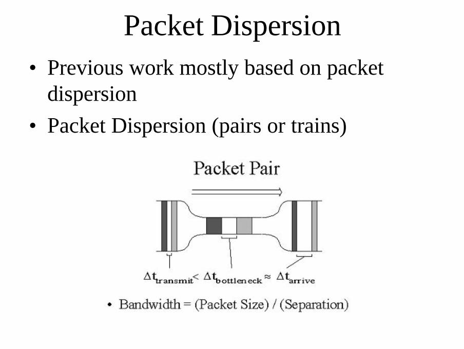
Packet Dispersion•Previous work mostly based on packet

dispersion •Packet Dispersion (pairs or trains)

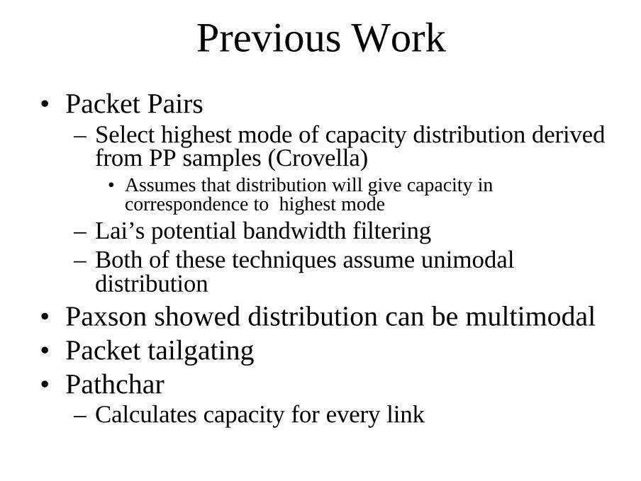
Previous Work•Packet Pairs

–Select highest mode of capacity distribution derived from PP samples (Crovella)

•Assumes that distribution will give capacity in correspondence to highest mode

–Lai’s potential bandwidth filtering –Both of these techniques assume unimodal

distribution•Paxson showed distribution can be multimodal•Packet tailgating•Pathchar

–Calculates capacity for every link

Previous Work

•Dovrolis’ Work–Explained under/over estimation of capacity

–Methodology•First send packet pairs•If multimodal, send packet trains

•Still no satisfactory solution!!!–Most techniques too complicated, time/bw-consuming,

inaccurate and prone to choice of parameters–Never tested on wireless

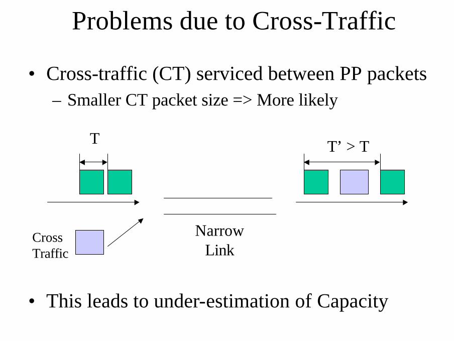
Problems due to Cross-Traffic

•Cross-traffic (CT) serviced between PP packets–Smaller CT packet size => More likely

•This leads to under-estimation of Capacity

Narrow Link

Cross Traffic

T T’ > T

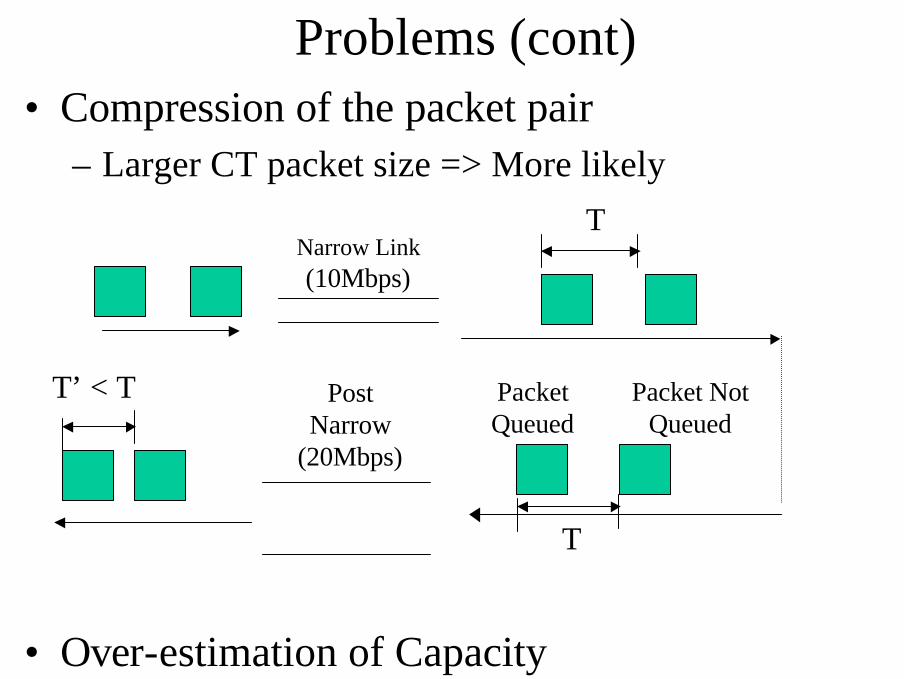
Problems (cont)•Compression of the packet pair

–Larger CT packet size => More likely

•Over-estimation of Capacity

Post Narrow

(20Mbps)

Narrow Link (10Mbps)

Packet Queued

Packet Not Queued

T

T

T’ < T

Fundamental Queuing Observation

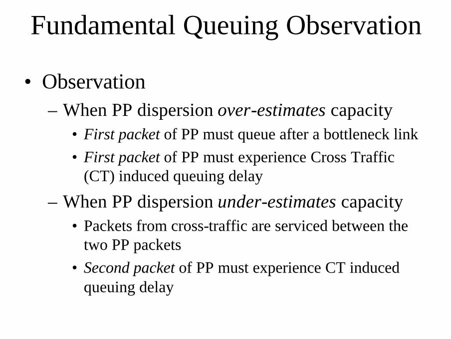
•Observation–When PP dispersion over-estimates capacity

•First packet of PP must queue after a bottleneck link•First packet of PP must experience Cross Traffic

(CT) induced queuing delay

–When PP dispersion under-estimates capacity•Packets from cross-traffic are serviced between the

two PP packets•Second packet of PP must experience CT induced

queuing delay

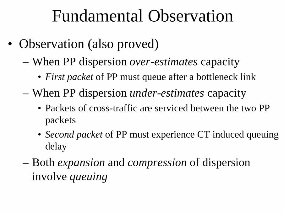
Fundamental Observation•Observation (also proved)

–When PP dispersion over-estimates capacity•First packet of PP must queue after a bottleneck link

–When PP dispersion under-estimates capacity•Packets of cross-traffic are serviced between the two PP

packets•Second packet of PP must experience CT induced queuing

delay

–Both expansion and compression of dispersion involve queuing

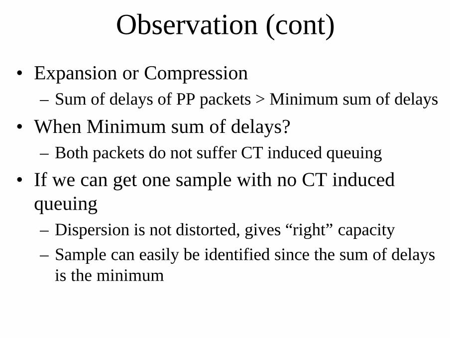
Observation (cont)

•Expansion or Compression–Sum of delays of PP packets > Minimum sum of delays

•When Minimum sum of delays?–Both packets do not suffer CT induced queuing

•If we can get one sample with no CT induced queuing–Dispersion is not distorted, gives “right” capacity–Sample can easily be identified since the sum of delays

is the minimum

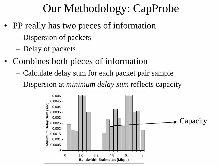
Our Methodology: CapProbe• PP really has two pieces of information

– Dispersion of packets– Delay of packets

• Combines both pieces of information– Calculate delay sum for each packet pair sample– Dispersion at minimum delay sum reflects capacity

Capacity

0

0.0005

0.001

0.0015

0.002

0.0025

0.003

0.0035

0.004

0.0045

0.005

0 1.6 3.2 4.8 6.4 8Bandwidth Estimates (Mbps)

Min

imu

m D

elay

Su

m (s

ec)

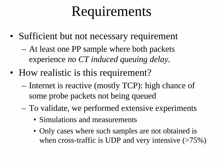
Requirements

•Sufficient but not necessary requirement–At least one PP sample where both packets

experience no CT induced queuing delay.

•How realistic is this requirement?–Internet is reactive (mostly TCP): high chance of

some probe packets not being queued–To validate, we performed extensive experiments

•Simulations and measurements•Only cases where such samples are not obtained is

when cross-traffic is UDP and very intensive (>75%)

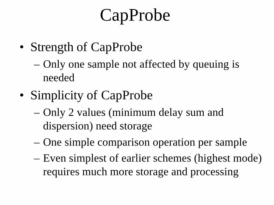
CapProbe

•Strength of CapProbe–Only one sample not affected by queuing is

needed

•Simplicity of CapProbe–Only 2 values (minimum delay sum and

dispersion) need storage–One simple comparison operation per sample–Even simplest of earlier schemes (highest mode)

requires much more storage and processing

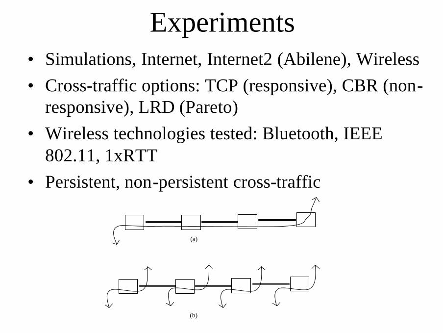
Experiments• Simulations, Internet, Internet2 (Abilene), Wireless• Cross-traffic options: TCP (responsive), CBR (non-

responsive), LRD (Pareto)• Wireless technologies tested: Bluetooth, IEEE

802.11, 1xRTT• Persistent, non-persistent cross-traffic

(a)

(b)

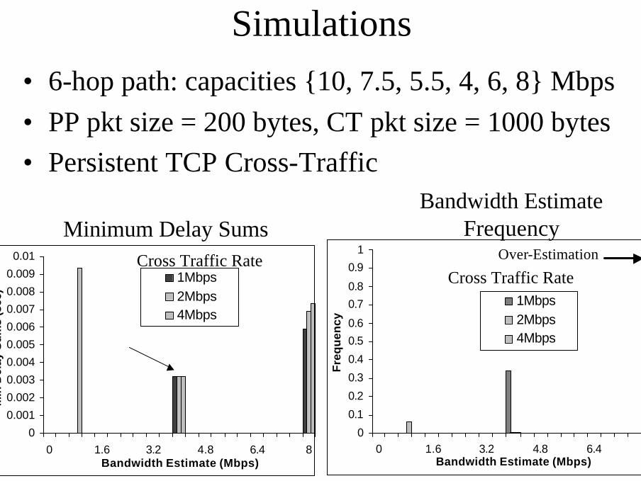
Simulations•6-hop path: capacities {10, 7.5, 5.5, 4, 6, 8} Mbps•PP pkt size = 200 bytes, CT pkt size = 1000 bytes•Persistent TCP Cross-Traffic

0

0.1

0.2

0.3

0.4

0.5

0.6

0.7

0.8

0.9

1

0 1.6 3.2 4.8 6.4 8Bandwidth Estimate (Mbps)

Fre

qu

ency

1Mbps2Mbps4Mbps

Over-Estimation

Cross Traffic Rate

Bandwidth Estimate Frequency

0

0.001

0.002

0.003

0.004

0.005

0.006

0.007

0.008

0.009

0.01


Min

Del

ay S

um

s (s

ec)

1Mbps2Mbps4Mbps

Cross Traffic Rate

Minimum Delay Sums

Simulations

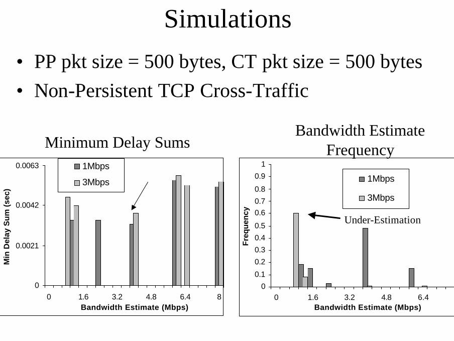
•PP pkt size = 500 bytes, CT pkt size = 500 bytes•Non-Persistent TCP Cross-Traffic

0

0.0021

0.0042

0.0063


Min

Del

ay S

um

(se

c)

1Mbps

3Mbps

Minimum Delay Sums

0

0.1

0.2

0.3

0.4

0.5

0.60.7

0.8

0.9

1


Fre

qu

ency

1Mbps

3Mbps

Under-Estimation

Bandwidth Estimate Frequency

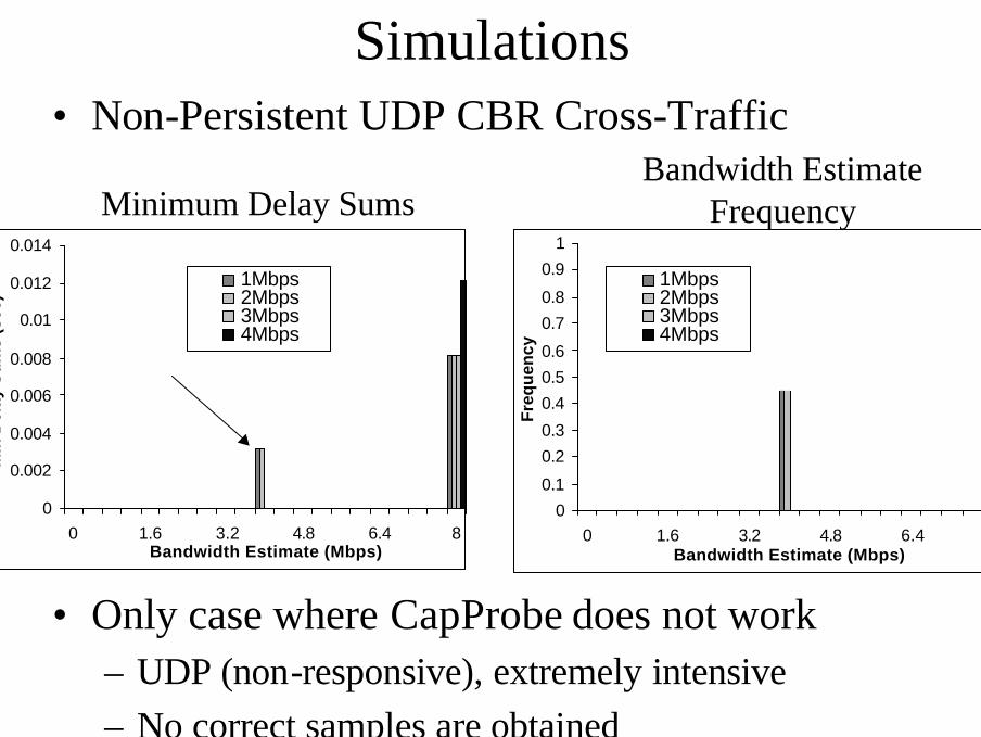
Simulations•Non-Persistent UDP CBR Cross-Traffic

•Only case where CapProbe does not work–UDP (non-responsive), extremely intensive–No correct samples are obtained

0

0.002

0.004

0.006

0.008

0.01

0.012

0.014


Min

Del

ay S

um

s (s

ec)

1Mbps2Mbps3Mbps4Mbps

0

0.1

0.2

0.3

0.4

0.5

0.6

0.7

0.8

0.9

1


Fre

qu

ency

1Mbps2Mbps3Mbps4Mbps

Minimum Delay SumsBandwidth Estimate

Frequency

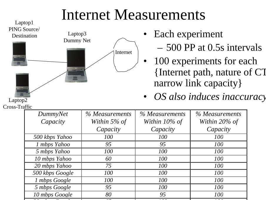
Internet Measurements• Each experiment

–500 PP at 0.5s intervals• 100 experiments for each

{Internet path, nature of CT, narrow link capacity}

• OS also induces inaccuracy

Laptop3 Dummy Net

Laptop1 PING Source/

Destination

Internet

Laptop2Cross-Traffic

DummyNet Capacity

% Measurements Within 5% of

Capacity


Capacity


Capacity 500 kbps Yahoo 100 100 100 1 mbps Yahoo 95 95 100 5 mbps Yahoo 100 100 100 10 mbps Yahoo 60 100 100 20 mbps Yahoo 75 100 100

500 kbps Google 100 100 100 1 mbps Google 100 100 100 5 mbps Google 95 100 100 10 mbps Google 80 95 100 20 mbps Google 65 100 100

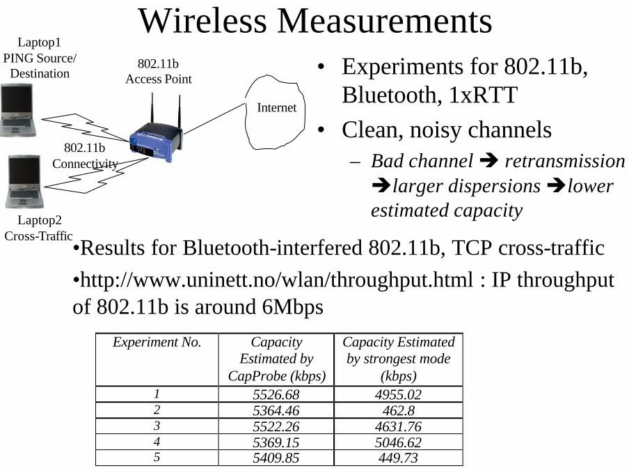
Wireless Measurements• Experiments for 802.11b,

Bluetooth, 1xRTT• Clean, noisy channels

– Bad channelè retransmissionèlarger dispersionsèlower estimated capacity

802.11bAccess Point

Laptop1 PING Source/

Destination

Internet

Laptop2Cross-Traffic

802.11bConnectivity

Experiment No. Capacity Estimated by

CapProbe (kbps)

Capacity Estimated by strongest mode

(kbps) 1 5526.68 4955.02 2 5364.46 462.8 3 5522.26 4631.76 4 5369.15 5046.62 5 5409.85 449.73

•Results for Bluetooth-interfered 802.11b, TCP cross-traffic•http://www.uninett.no/wlan/throughput.html : IP throughput of 802.11b is around 6Mbps

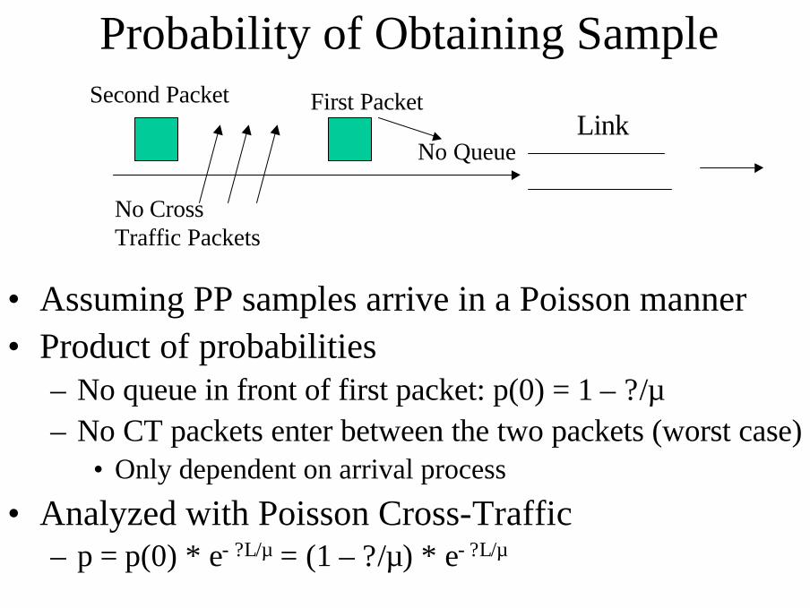
Probability of Obtaining Sample

•Assuming PP samples arrive in a Poisson manner•Product of probabilities

–No queue in front of first packet: p(0) = 1 –?/µ–No CT packets enter between the two packets (worst case)

•Only dependent on arrival process

•Analyzed with Poisson Cross-Traffic–p = p(0) * e- ?L/µ= (1 –?/µ) * e- ?L/µ

Link

No Cross Traffic Packets

First Packet

No Queue

Second Packet

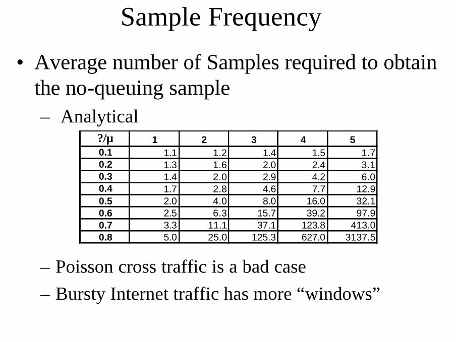
Sample Frequency

•Average number of Samples required to obtain the no-queuing sample– Analytical

–Poisson cross traffic is a bad case–Bursty Internet traffic has more “windows”

?/µ 1 2 3 4 50.1 1.1 1.2 1.4 1.5 1.70.2 1.3 1.6 2.0 2.4 3.10.3 1.4 2.0 2.9 4.2 6.00.4 1.7 2.8 4.6 7.7 12.90.5 2.0 4.0 8.0 16.0 32.10.6 2.5 6.3 15.7 39.2 97.90.7 3.3 11.1 37.1 123.8 413.00.8 5.0 25.0 125.3 627.0 3137.5

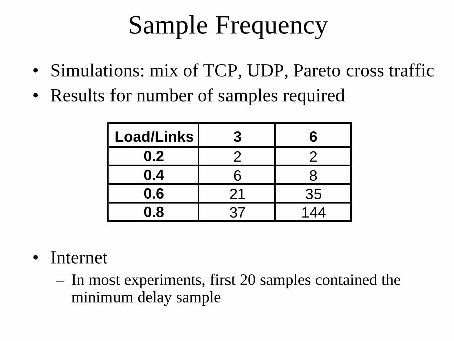
Sample Frequency

• Simulations: mix of TCP, UDP, Pareto cross traffic• Results for number of samples required

• Internet– In most experiments, first 20 samples contained the

minimum delay sample

Load/Links 3 60.2 2 20.4 6 80.6 21 350.8 37 144

Conclusion

•CapProbe–Simple capacity estimation method–Works accurately across a wide range of scenarios–Only cases where it does not estimate accurately

•Non-responsive intensive CT•This is a failure of the packet dispersion paradigm

•Useful application–Use a passive version of CapProbe with “modern”

TCP versions, such as Westwood

Estimating Bandwidth of Mobile Users

Documents

Transcript of Estimating Bandwidth of Mobile Users