Estimating aquifer hydraulic properties using sinusoidal ...

Estimating aquifer hydraulic properties using sinusoidal pumpingat the Savannah River site, South Carolina, USA

Todd C. Rasmussen · Kevin G. Haborak ·Michael H. Young

Abstract A framework for estimating aquifer hydraulicproperties using sinusoidal pumping is presented that (1)derives analytical solutions for confined, leaky, andpartially penetrating conditions; (2) compares the analyt-ical solutions with a finite element model; (3) establishesa field protocol for conducting sinusoidal aquifer tests;and (4) estimates aquifer parameters using the analyticalsolutions. The procedure is demonstrated in one surficialand two confined aquifers containing potentially contam-inated water in coastal plain sediments at the SavannahRiver site, a federal nuclear facility. The analyticalsolutions compare favorably with finite-element solu-tions, except immediately adjacent to the pumping wellwhere the assumption of zero borehole radius is not valid.Estimated aquifer properties are consistent with previousstudies for the two confined aquifers, but are inconsistentfor the surficial aquifer; conventional tests yieldedestimates of the specific yield—consistent with anunconfined response—while the shorter-duration sinuso-idal perturbations yielded estimates of the storativity—consistent with a confined, elastic response. The approachminimizes investigation-derived wastes, a significantconcern where contaminated fluids must be disposed ofin an environmentally acceptable manner. An additionaladvantage is the ability to introduce a signal differentfrom background perturbations, thus easing detection.

R�sum� Une d�marche pour estimer les propri�t�s d’unaquif�re � partir d’un d�bit de pompage � variationssinuso�dales est pr�sent�e pour (1) d�river des solutionsanalytiques pour des conditions captives, en drainance, etde puits incomplet convenant � plusieurs applicationspratiques, (2) v�rifier les solutions analytiques par rapport� un mod�le aux �l�ments finis, (3) �tablir un protocole deterrain pour r�aliser des essais d’aquif�re, et (4) estimerles param�tres de l’aquif�re � partir de solutions analy-tiques. Les solutions analytiques soutiennent bien lacomparaison avec les solutions aux �l�ments finis d’undomaine d’�coulement simul�, sauf dans les zonesimm�diatement voisines du puits de pompage o� l’hypo-th�se d’un rayon de forage nul n’est pas respect�e. Laproc�dure de terrain utilise (1) une cha�ne d’acquisitionde donn�es programmable que contr�lent des pompes �r�gime variable qui alternativement injectent et extraientl’eau du forage pour cr�er une impulsion sinuso�dale, (2)un conteneur mobile, au-dessus du sol qui stockemomentan�ment l’eau de l’aquif�re entre les cyclesd’extraction et d’injection, (3) des d�bitm�tres � palettesqui contr�lent les d�bits d’extraction et d’injection, et (4)des capteurs de pression qui contr�lent les niveaux d’eaudans les forages de pompage et d’observation. Laproc�dure est appliqu�e � une unit� aquif�re superficielleet � deux unit�s captives du site de la rivi�re Savannah, unsite nucl�aire f�d�ral de Caroline du Sud. L’approchesinuso�dale fournit rapidement des estimations des para-m�tres de l’aquif�re en �vitant les pertes de temps li�esaux �tudes.

Resumen Se presenta un marco para estimar las propie-dades de los acu�feros mediante una tasa de extraccinsinusoidal. El m�todo (1) deriva soluciones anal�ticas paracondiciones de acu�fero confinado, semiconfinado y depenetracin parcial, que son aplicables a muchas situa-ciones prcticas; (2) verifica las soluciones anal�ticas conun modelo de elementos finitos; (3) establece un proto-colo de campo para ejecutar ensayos hidrulicos; y (4)estima los parmetros del acu�fero por medio de lassoluciones anal�ticas. �stas han sido validadas de formasatisfactoria con soluciones num�ricas en un dominiosimulado de flujo, exceptuando las reas adyacentes alpozo de bombeo, para el que la hiptesis de radio nulo nose cumple. El procedimiento de campo utiliza (1) unregistrador de datos programable que controla las bombas

Received: 16 August 2002 / Accepted: 13 February 2003Published online: 24 April 2003

� Springer-Verlag 2003

T. C. Rasmussen ())School of Forest Resources, University of Georgia,1040 D.W. Brooks Drive, Athens, Georgia, 30602-2152, USAe-mail: [email protected].: +1-706-5424300Fax: +1-706-5428356

K. G. HaborakGolder International, 3730 Chamblee Tucker Road,Atlanta, Georgia, 30341, USA

M. H. YoungDivision of Hydrologic Sciences, Desert Research Institute,755 E. Flamingo Road, Las Vegas, Nevada, 89119, USA

Hydrogeology Journal (2003) 11:466–482 DOI 10.1007/s10040-003-0255-7

de velocidad variable que inyectan y extraen agua deforma alternativa desde el sondeo con el fin de crear unest�mulo sinusoidal; (2) un contenedor mvil, situado ensuperficie, que almacena temporalmente el fluido delacu�fero durante los ciclos; (3) contadores volum�tricostipo noria que registran las tasas de inyeccin y extrac-cin; y (4) transductores de presin para observar losniveles del agua en los sondeos de bombeo y control. Elprocedimiento ha sido verificado en un acu�fero superfi-cial y en dos niveles confinados del emplazamiento delr�o Savannah, en Carolina del Sur (Estados Unidos deAm�rica), donde se ubican unas instalaciones nuclearesfederales. El enfoque sinusoidal permite efectuar estima-ciones rpidas de los parmetros del acu�fero a la par queelimina residuos derivados de la investigacin.

Keywords Equipment · Field techniques · Hydraulictesting · Groundwater hydraulics · Hydraulic properties ·Sinusoidal testing

Introduction

Site characterization at locations with contaminatedgroundwater require hydraulic testing to determineaquifer hydraulic properties, primarily the aquifer trans-missivity, storativity, and leakage coefficient. Conven-tional aquifer tests rely on constant extraction of waterfrom, or injection into, a well bore with contemporaneousmonitoring of observation wells. The measured responsein the observation wells is then used to estimate aquiferhydraulic properties.

Aquifer tests that rely on groundwater pumping oftengenerate substantial volumes of water, which may becontaminated with hazardous chemicals. Due to potentialcontamination of these investigation-derived wastes, thewater may need to be collected, stored, treated, anddisposed of in an environmentally responsible manner atsubstantial costs.

A sinusoidal excitation of fluid pressure within thepumping borehole is an alternative method for aquifertesting. Advantages of the sinusoidal approach comparedto the constant flow aquifer test are: (1) investigation-derived wastes are eliminated, thus reducing disposalcosts for contaminated water, (2) the oscillating signal ofknown frequency is separable from changing backgroundpressure, (3) the time required to achieve steady condi-tions is shorter, and (4) it is theoretically possible toperform multiple tests simultaneously using uniquefrequencies for each of the source boreholes. Disadvan-tages of a sinusoidal test include: (1) measurable signalsmay not propagate as far into the aquifer as those from theconstant flow method, (2) there have been few publishedmethods of interpreting data from sinusoidal tests, and (3)more complex field instruments and pump controllers areneeded to conduct the aquifer test.

A sinusoidal pressure signal can be created with afixed period and amplitude. The pressure wave created bythis excitation diffuses into the aquifer and attenuates as it

diffuses. Observation boreholes are used to detect theamplitude attenuation and phase lag of the signal. Theattenuation and phase lag of the signal depend on thedistance of the observation boreholes from the pumpingborehole, the frequency of the sinusoidal excitation, andthe aquifer hydraulic properties.

The purpose of this paper is to present analyticalsolutions for sinusoidal aquifer tests, and to demonstratethe feasibility of the approach in three coastal-plainaquifers at the Savannah River site. Sinusoidal aquifer testsolutions are presented for confined (Theis 1935) andleaky (Hantush and Jacob 1955) aquifers for wells thatfully penetrate the aquifer, along with an analytic solutionfor confined aquifers with partially penetrating wells(Hantush 1964). A numerical model is compared to theanalytical solutions to evaluate the adequacy of theapproach. Finally, field test equipment is used to demon-strate the feasibility of the technique for a test wellcomplex at the Savannah River site. Interpretation of thesinusoidal aquifer test data is then provided using fielddata from the Savannah River site.

Background

An early method for determining aquifer hydraulicproperties for sinusoidal inputs was presented by Ferris(1963). This approach yields an estimate of aquifertransmissivity for a sinusoidal tidal input to a confined,one-dimensional (horizontal, x) flow domain. Gelhar(1974) presented the response in an aquifer to sinusoidalperturbations using three types of aquifer models: a linearreservoir model, a linear Dupuit aquifer, and a Laplaceaquifer. Flow in the first two cases occurs in a singlehorizontal, x, dimension, while the Laplace aquifer alsoincludes a vertical flow dimension, z. The form of thesesolutions precludes their use for interpreting radial flow toa borehole, r.

Black and Kipp (1981) were the first to provide asolution to an aquifer borehole test for a sinusoidalperturbation in a confined non-leaky aquifer. Solutionsare provided for both a point source (a well screened overa very small section relative to the entire thickness of anaquifer) and a line source (a well screened over the entirethickness of the aquifer). The approach uses the ratio ofeither the phase shift or amplitude from two observationwells to determine the aquifer hydraulic diffusivity.Unfortunately, their method does not provide the abilityto independently determine both the aquifer transmissiv-ity and storativity coefficient.

Natural excitations (such as precipitation, evapotran-spiration, barometric pressure, and tidal fluctuations)often show periodic behavior, making it possible to usesinusoidal analysis to determine aquifer hydraulic prop-erties. Approaches that use naturally occurring excitationsto estimate subsurface properties include barometricpressure perturbations (Rojstaczer 1988; Rojstaczer andRiley 1990; Rasmussen and Crawford 1997; Mehnert etal. 1999) as well as earth tide perturbations (Hsieh et al.

467


1987; Ritzi et al. 1991). These approaches take advantageof naturally occurring perturbations as the stimulus, andthen estimate aquifer properties using the observedresponse in a borehole. The magnitude of naturalexcitations is normally much smaller than those inducedduring aquifer tests.

One drawback of using natural excitations is thecomplexity of natural system behavior, often being amixture of processes including: (1) vertical transmissionof the barometric pressure stimulus through the unsatur-ated zone in the case of surficial aquifers, (2) verticaltransmission of surface loads through overlying units inconfined aquifers, (3) horizontal propagation within themonitored aquifer, and (4) borehole storage responses.Two advantages, therefore, of induced sinusoidal stimu-lation are that the system geometry can be simplified byremoving the vertical propagation from the earth’ssurface, and that a single frequency can be specified forexcitation.

Analytical Solutions

Analytical solutions are presented for sinusoidal equiva-lents of three steady-flow aquifer testing conditions: (1)the Theis (1935) solution of the confined aquifer problem,(2) the Hantush and Jacob (1955) solution of the leakyaquifer problem, and (3) the Hantush (1964) solution for apartially penetrating pumping well. The assumptions inthese models are that the aquifer is homogeneous,uniform in thickness, compressible and elastic, horizontal,and of infinite areal extent; groundwater flow is describedby Darcy’s law; pore fluids are elastic and of constantdensity and viscosity; the initial piezometric surface ishorizontal; the pumping well has an infinitesimal diam-eter; head losses through the well screen are negligible;and the pumping rate is constant.

Confined Aquifer SolutionTheis (1935) introduced an analytical solution for a wellpumping at a constant rate from a confined aquifersystem. The additional assumptions in the Theis solutionare that the aquifer is isotropic; groundwater flow ishorizontal; and the pumping well is fully penetrating.Black and Kipp (1981) introduced an analytical solutionfor a well pumping sinusoidally in a confined aquifersystem. The assumptions in this solution are identical tothose of the Theis solution with the exception of thepumping rate being sinusoidal. For the derivation of thesolution to the boundary value problem, the complexexponential function will be used to represent thesinusoidal pumping rate. The value of the complexexponential function is given by:

Q ¼ Qo eiwt ¼ Qo coswt þ i sinwt½ � ð1Þwhere Q is the complex pumping rate, Qo is the amplitudeof the pumping rate, w is the frequency of the excitation, tis a time variable, and i is the imaginary number. Usingthis representation has the advantage that the final

solution includes the response to both the real andimaginary components of the sinusoidal pumping rate.The final solution is a complex-valued function where thereal part is the response to the real component of thepumping rate and the imaginary part is the response to theimaginary component of the pumping rate (Saff andSnider 1993). Thus, the boundary value problem can bestated mathematically using:

@2s

@r2þ 1

r

@s

@r¼ 1

D

@s

@tð2Þ

s r; 0ð Þ ¼ 0 ð3Þ

s 1; tð Þ ¼ 0 ð4Þ

limr!0

r@s

@r¼ � Q

2p Tð5Þ

where D is the hydraulic diffusivity, s is the observeddrawdown, r is the distance from the pumping well, and Tis the aquifer transmissivity. The solution to this problem,derived in the Appendix, yields the steady periodicresponse to a sinusoidal pumping rate:

sðr; tÞ ¼ Q

2 pTKo r

ffiffiffiffiffi

iwD

r

!

ð6Þ

where Kois the zero-order modified Bessel function of thesecond kind. This solution neglects a nonperiodic, initial-transient component that decays with time after thebeginning of the sinusoidal aquifer test.

The amplitude of the water level fluctuations in anobservation well is:

jsj ¼ Qo

2 p TKo r

ffiffiffiffiffi

iwD

r

!�

�

�

�

�

�

�

�

�

�

ð7Þ

and the phase shift, f, is:

f ¼ arg Ko r

ffiffiffiffiffi

iwD

r

!( )

ð8Þ

This result is consistent with solution 215.08 inBruggeman (1999). These results are different in formbut consistent with the Black and Kipp (1981) solution.The results presented here are different because the Blackand Kipp solution employs a sinusoidal drawdown for theexcitation boundary instead of a sinusoidal flux boundarycondition. Introducing the flux boundary conditionsprovides the ability to estimate both the transmissivityand storativity using Eqs. (7) and (8). Barker (1988)presented an alternative Laplace transform solutionapproach to this problem.

Leaky Aquifer SolutionHantush and Jacob (1955) derived an analytical solutionfor a well pumping constantly from a leaky aquifersystem. The solution is appropriate for an aquifer that isbounded above or below by an aquiclude and bounded on

468


the opposing surface by an aquitard and a source aquifer.The additional assumptions in the Hantush and Jacobsolution are that the hydraulic conductivity of the aquitardis so small relative to the aquifers that flow in this layer isessentially vertical; the aquitard is incompressible; andthe water table in the source bed is horizontal and remainsconstant (therefore, the rate of leakage from the aquitardinto the pumped aquifer is directly proportional to thedrawdown at the interface).

The assumptions are identical to the Hantush andJacob assumptions, with the exception that the pumpingrate is sinusoidal:

@2s

@r2þ 1

r

@s

@r� s

B2¼ 1

D

@s

@tð9Þ

s r; 0ð Þ ¼ 0 ð10Þ

s 1; tð Þ ¼ 0 ð11Þ

limr!0

r@s

@r¼ � Q

2 p Tð12Þ

and where

B2 ¼ T

L¼ T m0

K 0ð13Þ

where L=K0/m0 is the aquifer leakance, and m0 and K0 arethe thickness and vertical hydraulic conductivity of theconfining layer, respectively. The steady periodic re-sponse to sinusoidal pumping in a leaky aquifer, asderived in the Appendix, is:

sðr; tÞ ¼ Q

2 p TKo r

ffiffiffiffiffiffiffiffiffiffiffiffiffiffiffiffi

iwDþ 1

B2

r

!

ð14Þ

where the nonperiodic, initial-transient response is ne-glected.

The amplitude of the water level response in anobservation well is:

jsj ¼ Qo

2 p TKo r


iwDþ 1

B2

r

!�

�

�

�

�

�

�

�

�

�

ð15Þ

and the phase shift is:

f ¼ arg Ko r


iwDþ 1

B2

r

!( )

ð16Þ

The result is consistent with Solution 215.18 inBruggeman (1999), except for a factor of two errors inthe Bruggeman solution, i.e., the denominator in Brugge-man should be 2pT instead of 4pT.

Partially Penetrating Well SolutionHantush (1964) presented a solution for a partiallypenetrating well pumping from a confined aquifer. Thesolution is appropriate for an aquifer bounded above andbelow by aquicludes. The additional assumptions in theHantush solution are that the aquifer is anisotropic; the

pumping well is partially penetrating (screened) from d tol; and the observation well is screened over the intervalfrom d’ to l’.

The assumptions are identical except that it is assumedthat the aquifer is isotropic and the pumping rate issinusoidal. This boundary value problem is expressedmathematically as:

@2s

@r2þ 1

r

@s

@rþ @

2s

@z2¼ 1

D

@s

@tð17Þ

s r; z; 0ð Þ ¼ 0 ð18Þ

s 1; z; tð Þ ¼ 0 ð19Þ

@s

@z

�

�

�

�

z¼0

¼ 0 ð20Þ

@s

@z

�

�

�

�

z¼m

¼ 0 ð21Þ

limr!0

r@s

@r¼

0 0 � z < d� Q

2pKðl�dÞ d � z � l0 l < z � m

8

<

:

ð22Þ

where m is the aquifer thickness, K is the aquiferhydraulic conductivity, l and d are the upper and lowerlimits of the screened zone within the pumping well,respectively, and l’ and d’ are the upper and lower limitsof the screened zone in the observation well, respectively.The steady periodic solution to sinusoidal pumping in aconfined aquifer with a partially penetrating well, asderived in the Appendix, is:

sðr; l0; d0; tÞ ¼ Q

2pTKo r

ffiffiffiffiffi

iwD

r

!(

þ 2m2

p2ðl� dÞðd0 � l0Þ

Z

1

n¼1

1n2

sinnpl

m� sin

npd

m

� ��

Ko r

ffiffiffiffiffiffiffiffiffiffiffiffiffiffiffiffiffiffiffiffiffiffi

iwDþ np

m

h i2r

!

sinnpl0

m� sin

npd0

m

� �

!!

ð23Þ

where the nonperiodic, initial-transient components areagain neglected. The amplitude of the water levelresponse in an observation well is:

jsj ¼ Qo

2pTKo r

ffiffiffiffiffi

iwD

r

!�

�

�

�

�

þ 2m2


Z

1

n¼1

1n2

sinnpl

m� sin

npd

m

� ��

Ko r


iwDþ np

m

h i2r

!

sinnpl0

m� sin

npd0

m

� �

!!

ð24Þ

and the phase shift of the response is

469


f ¼ arg Ko r

ffiffiffiffiffi

iwD

r

!(

þ 2m2


Z

1

n¼1

1n2

sinnpl

m� sin

npd

m

� ��

Ko r


iwDþ np

m

h i2r

!

sinnpl0

m� sin

npd0

m

� �

!!

ð25Þ

This solution has not been derived elsewhere.

Comparison with a Numerical Model

An axisymmetric, linear, triangular, finite-element modelwas developed using Matlab 5.2 to provide numericalsolutions for comparison with the analytical solutionspresented above. The model is used to provide greaterconfidence in, and a better understanding of, the analyticsolutions.

The consistent formulation of Galerkin’s method ofweighted residuals is used for both s and @s/@t, using alinear variation with r and z (Segerlind 1984; Cheney andKincaid 1994), while the trapezoid rule is used tointegrate with respect to time. The generated mesh isfiner near the pumping well boundary and becomescoarser with increasing radial distance. The mesh alongthe r-axis ranges from 0.03 to 1,000 m, while the z-axisranges from 0 to 100 m. A mesh refinement program wasused to increase the spatial density of nodes from aninitial specification of 103 vertices and 169 triangles to afinal geometry of 5,549 vertices and 10,816 triangles(Haborak 1999).

Boundary conditions were established for confined andleaky aquifers, as well as for a well that partiallypenetrates a confined aquifer. A pumping rate of 500 m3/day, a frequency of three cycles/day (i.e., an 8-h period), astorativity of 1.6 10�6, and a transmissivity of 51 m2/daywere specified for all simulations. The source well wasfully screened between 35 and 60 m for the partiallypenetrating well problem. For the leaky case, the aquitardhydraulic conductivity was set at 0.03 m/day and theaquitard thickness was 10 m.

Two initial conditions were specified for each of theboundary value problems: (1) the initial drawdown is zero

throughout the domain, and (2) the initial drawdown isequal to the analytical solution value at t=0 (simulatingsteady periodic conditions). The two initial conditionswere used to evaluate the effect of the neglected initialtransient terms in the analytical solution. The duration ofthe pumping period was set at 30 h using a time step of3 min (600 time steps total). The solutions of theproblems required a total of approximately 40 min on a266-MHz Pentium II with 64 MB of RAM. The numericaland analytical predictions of drawdown were compared att=6, 7.5, 10, 15, and 30 h.

Table 1 presents the root-mean squared differencesbetween the numerical and analytical solutions within themodeled domain at nodes less than and greater than 2 mfrom the pumping well, expressed as the percentage of theanalytical solution, for the case where the initial draw-down is zero. The division of nodes into two groups (i.e.,less than and greater than 2 m from the pumped well) wasmade based on inspection of calculated errors—errors atnodes within 2 m were generally greater than errors atnodes outside of this zone.

The excellent agreement between numerical andanalytical solutions, even within the 2-m zone, suggeststhat the analytical steady periodic solutions are consistentwith the numerical model. Differences for the case wherethe initial condition were specified equal to the analyticalsolution are practically identical to those presented inTable 1, indicating that the effects of the initial transientcan be neglected.

Nodes closer than 2 m show greater differencesbecause of the assumption of an infinitesimal welldiameter used to obtain the analytical solution. Thisassumption causes the analytical solution to approachinfinity as the radial distance approaches zero; therefore,the analytical solutions do not accurately represent thephysical system near the pumping well. Larger differ-ences were found for the case where the initial conditionwas set equal to zero (e.g., 4.4% vs. 0.2% for the confinedaquifer at distances greater than 2 m at 6 h), but thesedifferences decreased by the end of the simulation period(e.g., 0.6% vs. 0.1% for the confined aquifer at distancesgreater than 2 m at 30 h), presumably due to the decay ofthe initial transient. It is also interesting to note that thedifferences for the confined aquifer at large distance arelarger than for either the leaky or partially penetratingcases.

Table 1 Root-mean-squared differences between analytical solutions and finite-element simulation models, expressed as a percentage ofthe analytical solution

Time (h) Nodes within 2 m of pumped well Nodes beyond 2 m of pumped well

Confinedaquifer

Leakyaquifer

Partially penetratingaquifer

Confinedaquifer

Leakyaquifer

Partially penetratingaquifer

6 9.2 8.4 13.3 4.4 0.1 0.97.5 7.5 6.5 10.5 5.4 0.1 0.6

10 7.9 8.4 12.8 2.8 0.1 0.915 7.0 7.5 11.4 2.0 0.1 0.730 8.0 8.4 12.9 0.6 0.1 0.9

470


Field Demonstration

Site DescriptionSinusoidal aquifer tests were conducted at the SouthwestPad, shown in Fig. 1, which is located near the BurialGround Complex at the Savannah River site. TheSavannah River site is located in the Atlantic CoastalPlain physiographic province, which extends from CapeCod, Massachusetts, to south-central Georgia. Thisprovince is underlain by seaward-dipping unconsolidatedand poorly consolidated sediments that, in South Caroli-na, increase from a thickness of zero at the Fall Line (i.e.,the uppermost extent of the Coastal Plain province) tomore than 1,200 m at the coast. The sediments of theAtlantic Coastal Plain were deposited under a variety ofconditions and have formed a complex system oftransmissive and confining units. The Savannah Riversite is located near the updip edge of the Atlantic CoastalPlain sequence where the sedimentary wedge thinsdramatically and undergoes abrupt facies changes (Aad-land et al. 1995).

Table 2 presents the litho- and hydro-stratigraphy inthe vicinity of the aquifer testing location. The FloridanAquifer system is the uppermost system at the SavannahRiver site, and is the subject of investigation here.Tables 3 and 4 present representative values of selectedhydrologic properties for aquifers and confining units,respectively, in the vicinity of the aquifer testing location(Aadland et al. 1995).

The Gordon Aquifer is the deepest aquifer within theFloridan Aquifer system and has a thickness that ranges

from 20 to 30 m. The Green Clay Aquitard separates theGordon Aquifer from the overlying Upper Three RunsAquifer. The Green Clay, present at a depth between 30and 50 m, includes abrupt facies changes from clay tosilty and sandy material, with a thickness ranging from0.6 to 3 m. The permeability of this unit varies greatly;

Table 2 Representative litho- and hydro-stratigraphy of the Savannah River site

Lithostratigraphy Hydrostratigraphy

Age Group Formation Unit System

Miocene Hawthorne Altamaha (Upland) Surficial Aquifer Floridan Aquifer system

Eocene Barnwell Tobacco RoadIrwinton Sanda

Twiggs Claya Tan Clay AquitardGriffins Landinga Barnwell-McBean AquiferClinchfield

Orangeburg Tinker/SanteeWarley Hill Green Clay AquitardCongaree Gordon Aquifer

Black Mingo Fishburne/Fourmile

Paleocene Snapp/Williamsburg Crouch Branch Aquitard Meyers Branch Confining systemEllenton

Cretaceous Lumbee Steel Creek/Peedee Crouch Branch Aquifer Dublin-Midville Aquifer systemBlack Creek

a Members of Dry Branch Formation

Fig. 1 General location map for the Southwest Pad, Burial GroundComplex, Savannah River site

Table 3 Representative hydro-logic properties of aquifers,Burial Ground Complex,Savannah River site

Aquifer Thickness(m)

Diffusivity, D(m2/s)

Transmissivity, T(m2/s)

Storativity, S

Surficial 3–12 0.07 0.8 10�3 120 10�4

Barnwell-McBean 12–40 4 0.6 10�3 1.6 10�4

Gordon 20–30 10 2.5 10�3 2.5 10�4

Crouch Branch 75 78 31 10�3 4.0 10�4

471


zones within this unit can be locally confining, semi-confining (leaky), or transmissive.

The Upper Three Runs Aquifer lies above the GreenClay Aquitard, and is subdivided into an Upper Unit and aLower Unit. The Lower Unit is commonly referred to asthe Barnwell-McBean Aquifer, and is a poorly defined,semi-confined aquifer ranging in thickness from 12 to40 m. This aquifer consists mainly of sands and fine-grained material, but limestone can be found in the lowersection of the unit. The Tan Clay Aquitard separates theUpper and Lower Units. The Tan Clay is a semi-confining(leaky) layer formed by lenses of clay and sandy clay,ranging in thickness from 0 to 8 m. The Upper Unit (alsocalled the Surficial Aquifer) is an unconfined aquifer thatlies above the Tan Clay, and is encountered at depthsdown to 25 m below ground surface, and varies insaturated thickness from 3 to 12 m.

Precipitation recharges the Surficial Aquifer, anddischarge occurs by leakage into underlying aquifers aswell as by seepage into local perennial streams to thenorth and south. Flow into and through underlyingaquifers also migrates to regional discharge points inmore distant rivers and streams.

All three aquifers within the Floridan Aquifer Systemwere examined in this study. The test facility contains onepumping well within each aquifer of the three aquifers,along with two observation wells in the Surficial Aquiferand the Barnwell-McBean Aquifer, and three observationwells in the Gordon Aquifers. Figure 2 presents plan andprofile views of the Southwest Pad configuration.

EquipmentThe field testing equipment was designed to honor severalobjectives, including: (1) the incorporation of off-the-shelf components, (2) the need for portability and ease offield setup, and (3) the need to constrain costs. Becausetechnology transfer from this research project to thegeneral public was an important consideration, it wasbelieved that honoring the above objectives wouldfacilitate use by others.

Figure 3 is a schematic of the field setup. The controland monitoring system was designed around the CR23Xdatalogger (Campbell Scientific, Inc., Logan, UT). Thedatalogger is equipped with digital input–output controlports, and differential analog- and constant-voltage chan-nels for controlling and monitoring pressure transducers,solenoid valves, flow meters, and pumping rates. Thedatalogger has an RS-232 port that allows continuousmonitoring with a portable computer. The datalogger wasprogrammed to minimize power usage during operations

so that a single, deep-cycle marine battery provided amplepower for the datalogger operation.

Sinusoidal pumping rates were controlled using aVariable Frequency Drive (VFD, Model Redi-Flo, Grund-fos Pumps Corp., Clovis, CA), which provides 120 VACpower for the pumps. The frequency response (w) of theVFD was controlled by a 4- to 20-mA signal convertedfrom voltage output of the datalogger (€5 V) using asignal control module (model SCM5B39–2, Dataforth,Tucson, AZ). The range of frequencies available to thepumps ranged from 0 to 100 Hz. Sensitivity of thepumping control system (i.e., dw/dV) was determined tobe 10.2€0.005 Hz/V.

Two Grundfos, 10-cm (4-inch) Redi-Flow VariablePerformance Pumps (model 16E4, Grundfos PumpsCorp., Clovis, CA) were used in the field. The first pumpwas used for withdrawing water from the target well, andthe second pump was used for reinjection. The reinjectionpump was installed horizontally in a portable, 79-m3

container (Rain for Rent, Charlotte, NC) and securedwith concrete blocks. At least 20 cm of water wasmaintained above the pump intake to prevent cavitation.The 16E4 pumps are capable of flows that range from 0.1to 92.6 L/min, depending on the dynamic head losses andthe frequency settings on the VFD.

Flow rates in each direction were monitored withseparate flow meters (model FP5300, Omega Engineer-ing, Stamford, CT) connected to the datalogger throughmagnetic amplifiers (model FLSC-AMP-A, Omega En-gineering) that filter high-frequency noise and boostsignal output. Withdrawal and injection flow lines wereopened and closed using normally closed, zero-differen-tial solenoid valves (model S20, GC Valves, Simi Valley,CA). The valves fully seal when de-energized without theneed for backpressure, a requirement in this field setupwhere backpressure on both the pumping and injectiondirections would range from 0 to 3 m maximum.

Powering the system required the use of several relays,all controlled by the datalogger. A double-throw latchingrelay (model HD4850, Crydom, San Diego, CA) wasenergized by the datalogger to turn the VFD on and off,which was needed before switching flow directions. Thesecond set of relays (all model D2425, Crydom) split theAC power cable from the VFD to the pumps. Because thepumps required three-phase power, three relays wereneeded for each pump, which were energized by a fourthrelay (model D1D07, Crydom) controlled by the datalog-ger. The relays, mounted on a single board, made thepurchasing of a second VFD unnecessary, reducingequipment costs by several thousand dollars. A third setof relays (model D1D07) energized the two solenoid

Table 4 Representative hydro-logic properties of confiningunits, Burial Ground Complex

Confining unit Thickness, m0

(m)Vertical hydraulic conductivity, K’(m/s)

Leakance, L=K0/m0

(L/s)

Tan Clay 1.5–8 2.11 10�9 3.0 10�10

Green Clay 0.6–3 0.64 10�9 3.2 10�10

Crouch Branch 18 1.10 10�9 0.58 10�10

472


valves. All relays were DC powered by a single, deep-cycle marine battery. A 30-amp portable generatorsupplied AC power to the pumps.

Pressure transducers (model PDCR 1830-8388, Druck,Inc., New Fairfield, CT) were installed inside thepumping well and portable water container to monitorchange in water levels, and for calculations of head lossduring the aquifer tests. Additional gauge pressuretransducers (model PDCR 830-0576, Druck, Inc., NewFairfield, CT) were tied to multiple CR-10 dataloggers(Campbell Scientific, Inc., Logan, UT) installed at all

monitoring wells. In addition to monitoring water levelsin each of the pumping wells (SWP 100D, SWP 200C,and SWP 300A), two observation wells (SWP 101D andSWP 102D) were used to monitor water levels in theSurficial Aquifer, two in the Barnwell-McBean Aquifer(SWP 201C and SWP 202C), and three in the GordonAquifer (SWP 301A, SWP 302A, and SWP 303A).

Fig. 2 Site configuration for theSouthwest Pad: a plan view, bprofile view

473


Aquifer Test Interpretation

Aquifer Test ConditionsTable 5 presents the aquifer test conditions for thesinusoidal aquifer tests in each of the three aquifersevaluated. Note that multiple cycles were used to obtainrepetitions of each complete cycle. The first step inaquifer test interpretation is to fit the pumping well flowrate using ordinary least squares. This is done byestablishing the sinusoidal function as:

QðtÞ ¼ Q1 coswt þ Q2 sinwt ð26Þwhere w=2p/p is the specified frequency of the inducedpumping, p is the pumping cycle period, and t is the timefrom the beginning of the aquifer test. In this case, thepumping rate, Q(t) and the cosine and sine terms areknown, and the objective is to estimate the unknowncoefficients, Q1 and Q2. The amplitude, Qo, and phase lag,jQ, of the pumping rate are then calculated using:

Qo ¼ jQj ¼ffiffiffiffiffiffiffiffiffiffiffiffiffiffiffiffiffi

Q21 þ Q2

2

q

ð27Þ

fQ ¼ atanQ2

Q1ð28Þ

Aquifer drawdowns in observation wells are also fit usingsinusoidal functions in the same manner.

sðtÞ ¼ s1 coswt þ s2 sinwt ð29ÞTo simplify interpretation, the amplitude and phase lag

of observation-well drawdowns were further adjusted toyield unit drawdowns that corresponds to the drawdownamplitude and phase lag corresponding to a unit (cosine)pumping rate:

so ¼jsjjQj ¼

ffiffiffiffiffiffiffiffiffiffiffiffiffiffi

s21 þ s2

2

p

ffiffiffiffiffiffiffiffiffiffiffiffiffiffiffiffiffi

Q21 þ Q2

2

p ð30Þ

fo ¼ fs � fQ ¼ atans2

s1� atan

Q2

Q1ð31Þ

where so is the drawdown amplitude per unit pumpingamplitude and jo is phase lag between the observeddrawdown and the imposed pumping. If needed, the phaselag can also be expressed in units of radians by dividingthe phase lag expressed in units of time by the pumpingfrequency, i.e., f (rad)=f (time)/w.

Figure 4 presents the observed pumping rates, Q, anddrawdowns, s, along with best-fit sinusoidal functions.Table 6 summarizes pumping data and water level

Fig. 3 Field configuration andwiring diagram for sinusoidalaquifer test

Table 5 Sinusoidal aquifer testconditions, Southwest Pad

Aquifer Pumped well Period, p(h)

Cycles(n)

Pumping rate amplitude, |Q|(L/s)

Surficial SWP 100D 1 4 0.416Barnwell-McBean SWP 200C 2 4 1.190Gordon SWP 300A 2.5 3 1.079

474


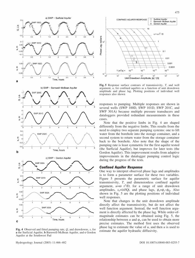
responses to pumping. Multiple responses are shown inseveral wells (SWP 100D, SWP 101D, SWP 201C, andSWP 301A) because multiple pressure transducers anddataloggers provided redundant measurements in thesecases.

Note that the positive limbs in Fig. 4 are shapeddifferently from the negative limbs. This results from theneed to employ two separate pumping systems: one to liftwater from the borehole into the storage container, and asecond system to return water from the storage containerback to the borehole. Also note that the shape of thepumping rate is least symmetric for the first aquifer tested(the Surficial Aquifer), but improves for later tests (theGordon Aquifer). This improvement results from adaptiveimprovements in the datalogger pumping control logicduring the progress of the tests.

Confined Aquifer ResponseOne way to interpret observed phase lags and amplitudesis to form a parameter surface for these two variables.Figure 5 presents the parametric surface for aquifertransmissivity, T, and dimensionless confined aquiferargument, u=w r2/D, for a range of unit drawdownamplitudes, so=|s|/|Q|, and phase lags, fo=fs�fQ. Alsoshown in Fig. 5 are the plotting positions of individualwell responses.

Note that changes in the unit drawdown amplitudedirectly affect the transmissivity, but do not affect thewell function argument. Instead, the well function argu-ment is directly affected by the phase lag. While order-of-magnitude estimates can be obtained using Fig. 5, therelationship between u and jo can be used to obtain moreprecise estimates. The method first uses the observedphase lag to estimate the value of u, and then u is used toestimate the aquifer hydraulic diffusivity.Fig. 4 Observed and fitted pumping rate, Q, and drawdowns, s, for

a the Surficial Aquifer, b Barnwell-McBean Aquifer, and c GordonAquifer at the Southwest Pad

Fig. 5 Response surface contours of transmissivity, T, and wellargument, u, for confined aquifers as a function of unit drawdownamplitude and phase lag. Plotting positions of individual wellresponses also shown

475


The aquifer hydraulic diffusivity for a confined aquiferis estimated using Eq. (8), which specifies the relationshipbetween the phase lag, fo, the pumping frequency, w, thedistance from the pumping well, r, and the hydraulicdiffusivity, D. This relationship can be written as:

fo ¼ FðuÞ ¼ arg Ko

ffiffiffiffi

iup� �n o

ð32Þ

where u is the principal unknown. Given that the phaselag has already been calculated using Eq. (31), thisequation can be solved for u by inversion to obtain aunique estimate of the well function, u=F�1 (fo), in whichthe inverse function is approximated using a fifth-order,logarithmic polynomial:

ln u ¼Z

5

i¼o

ci ðln foÞi ð33Þ

where c=[�0.12665, 2.8642, �0.47779, 0.16586,�0.076402, 0.03089].

Thus, the first step is to use the estimated phase lag inEq. (31) to obtain u. The aquifer diffusivity, D, is thenreadily found using:

D ¼ w r2

uð34Þ

The aquifer transmissivity, T, is then determined byrearranging Eq. (7):

T ¼jQj Koð

ffiffiffiffi

iupÞ

�

�

�

�

2pjsj ¼Koð

ffiffiffiffi

iupÞ

�

�

�

�

2psoð35Þ

Finally, the aquifer storativity is found using S=T/D.Tables 7 and 8 summarize the estimated aquifer

parameters, arranged by aquifer. It is interesting to notethe small values of the aquifer storativity for the SurficialAquifer. In effect, the aquifer test period is too short toinduce delayed yield, and appears to only induce elasticstorage of water. All aquifers were treated as confined,even the Surficial Aquifer. The use of a confined modelfor the Surficial Aquifer is justified in this analysis fortwo reasons: (1) the amplitude of the disturbance in theSurficial Aquifer is small (less than 3% of the thickness ofthe aquifer), and (2) the calculated aquifer storativity isvery small, less than 3 10�4, which is consistent withconfined behavior.

Table 6 Observed water level responses to sinusoidal pumping. Well ID: D Surficial Aquifer; C Barnwell-McBean Aquifer; A GordonAquifer

Well ID Well radius(cm)

Well distance(m)

Screen zone Datalogger Unit drawdownamplitudea

(s/m2)

Phase lag(min)

Elevation(m, a.m.s.l.)

Length(m)

SWP 100D 7.6 0.0 63.5 9.1 CR-23 7,828 1.77CR-10 7,485 1.79

SWP 101D 2.5 6.1 60.7 3.0 CR-23 219 2.53CR-10 223 2.92

SWP 102D 2.5 11.5 62.5 3.0 CR-10 151 3.49SWP 200C 7.6 0.0 45.9 18.3 CR-23 6,613 3.72SWP 201C 2.5 6.3 39.0 3.0 CR-23 2,568 10.81

CR-10 2,055 10.86SWP 202C 2.5 30.1 48.7 3.0 CR-10 234 37.05SWP 300A 5.1 0.0 26.4 12.2 CR-23 4,169 4.53SWP 301A 2.5 5.5 23.0 3.0 CR-23 371 5.41

CR-10 350 5.93SWP 302A 2.5 60.6 27.6 3.0 CR-10 17 31.33SWP 303A 2.5 139.8 30.4 3.0 CR-10 10 43.66

a Unit drawdown amplitude is the amplitude of the water level change divided by the amplitude of the pumping rate, |s|/|Q|

Table 7 Summary of parameterestimates for sinusoidal aquifertests. Well ID: D SurficialAquifer; C Barnwell-McBeanAquifer; A Gordon Aquifer

Well ID Datalogger u D(m2/s)

T(m2/s)

S

SWP 101D CR-23 4.01 10�3 16.07 21.7 10�4 1.35 10�4

CR-10 9.13 10�3 7.09 18.5 10�4 2.61 10�4

SWP 102D CR-10 23.10 10�3 9.96 22.7 10�4 2.28 10�4

SWP 201C CR-23 0.239 0.15 0.69 10�4 4.74 10�4

CR-10 0.242 0.14 0.85 10�4 5.97 10�4

SWP 202C CR-10 5.52 0.14 1.02 10�4 7.10 10�4

SWP 301A CR-23 1.41 10�3 14.85 15.0 10�4 1.01 10�4

CR-10 2.64 10�3 8.03 14.7 10�4 1.83 10�4

SWP 302A CR-10 1.86 1.38 37.0 10�4 26.8 10�4

SWP 303A CR-10 4.29 3.56 30.8 10�4 8.64 10�4

476


Leaky Aquifer ResponseThe effect of leakage on aquifer parameters was evaluatedqualitatively by comparing observed drawdown ampli-tudes and phase lags with leaky aquifer response curves.Response curves are constructed so that all aquifer testscan be compared on a single plot. Leaky aquifer responsecurves can be constructed for a range of well arguments,u, and leakage, n=(r/B)2, using Eq. (15):

se ¼ Koðffiffiffiffiffiffiffiffiffiffiffiffi

iuþ np

Þ�

�

�

� ð36Þwhere se=2p T |s|/|Q| is the dimensionless drawdownamplitude. The confined aquifer model can be used toprovide an initial estimate of the aquifer transmissivity,i.e., Eq. (35).

Plots of dimensionless drawdown amplitude and phaselags are shown in Fig. 6, along with response curves forrepresentative values of n=0.1, 0.01, and 0.0001. Inspec-tion of the figure indicates that increasing the leakageparameter causes the response curve to shift to the left(i.e., lower dimensionless drawdown amplitudes) forsmaller phase lags. The effects of leakage should manifestthemselves by displaying a smaller dimensionless draw-down amplitude when the phase lag is small.

Observed aquifer responses for sinusoidal tests con-ducted at the Southwest Pad tend to fall along theconfined aquifer type curve (n=0), and none of the leakyaquifer type curves appear to match observed amplitudes.Leakage between units cannot be estimated from the data,and longer period cycles are required if estimates ofaquifer leakage are needed.

While the most distant points (i.e., the observationwells with the smallest amplitudes and largest phase lags)fall below the confined aquifer curve, this is more likelydue to spatial heterogeneity within the aquifer than due tothe effects of leakage. As shown in the profile view inFig. 2, well screens in observation wells located awayfrom the pumped well (Wells SWP 302A and 303A) arepositioned above a clay lens, while the well screen in thenearest well (Well SWP 301A) lies below the clay lens.

Partially Penetrating Aquifer ResponseThe observation wells at the Southwest Pad only partiallypenetrate the aquifer. Parameter estimate should not beaffected when the pumping well fully penetrates aconfined aquifer with no leakage. In other situations,

however, the pumping well screen may not fully span theaquifer, and the hydraulic response at observation wellsmay be affected.

The magnitude of the effects of a partially penetratingpumping and/or observation well depends on the config-uration of the pumping and observation well screens. As aresult, a response curve that applies to all configurationsis substantially more difficult to construct. Instead, knownscreen lengths and positions can be used to generateresponse curves for the specific problem of concern usingEq. (23).

As an exercise, the effects of partial penetration wereevaluated at the Southwest Pad. Observation wellscreened intervals are all 3 m in length. The screenedzone in the pumping wells is 9.1 m for the SurficialAquifer (Well SWP 100D), 18.3 m for the Barnwell-McBean Aquifer (Well SWP 200C), and 12.2 m for theGordon Aquifer (Well SWP-300A).

Figure 6 shows the confined aquifer response curvealong with partial penetration response curves corre-sponding to aquifer conditions at the Southwest Pad. Notethat in all cases the response curves corresponding topartial penetration overlay the confined aquifer curve.Clearly, the effects of partial penetration are not importantfor the field conditions at the Southwest Pad when asinusoidal pumping rate is used.

If the effects of partial penetration are a concern, thena response curve can be constructed for known aquiferand well-screen geometries. The computed responsecurve should then be used instead of Eq. (32). Theaquifer hydraulic diffusivity can be estimated using a newform of Eq. (33) for the problem of interest, and thetransmissivity estimated using the form analogous toEq. (35). The aquifer storativity is again estimated usingS=T/D.

Table 8 Summary of parameter estimates for constant-dischargeaquifer tests. Well ID: D Surficial Aquifer; C Barnwell-McBeanAquifer; A Gordon Aquifer

Well ID D(m2/s)

T(m2/s)

S

SWP 101D 40.83 9.80 10�4 0.24SWP 102D 31.38 8.16 10�4 0.26SWP 201C 0.09 0.78 10�4 8.77 10�4

SWP 202C 0.27 1.29 10�4 4.86 10�4

SWP 301A 0.67 5.18 10�4 7.72 10�4

SWP 302A 1.36 25.35 10�4 18.7 10�4

SWP 303A 3.72 24.46 10�4 6.57 10�4

Fig. 6 Response curves for leaky aquifers (above) and thepredicted effects of partial penetration at the Southwest Pad (below)

477


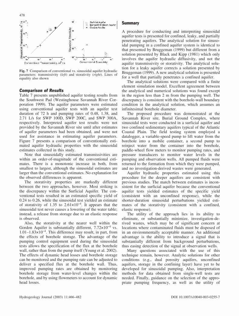
Comparison of ResultsTable 7 presents unpublished aquifer testing results fromthe Southwest Pad (Westinghouse Savannah River Cor-poration 1999). The aquifer parameters were estimatedusing conventional aquifer tests with an aquifer testduration of 72 h and pumping rates of 0.48, 1.38, and2.71 L/s for SWP 100D, SWP 200C, and SWP 300A,respectively. Interpreted aquifer test results were notprovided by the Savannah River site until after estimatesof aquifer parameters had been obtained, and were notused for assistance in estimating aquifer parameters.Figure 7 presents a comparison of conventionally esti-mated aquifer hydraulic properties with the sinusoidalestimates collected in this study.

Note that sinusoidally estimated transmissivities arewithin an order-of-magnitude of the conventional esti-mates. There is a monotonic increase in both, fromsmallest to largest, although the sinusoidal estimates arelarger than the conventional estimates. No explanation forthe observed differences is apparent.

The storativity properties are markedly differentbetween the two approaches, however. Most striking isthe discrepancy within the Surficial Aquifer. The con-ventional tests resulted in an estimated specific yield of0.24 to 0.26, while the sinusoidal test yielded an estimateof storativity of 1.35 to 2.61 10�4. It appears that thesinusoidal test never causes a lowering of the water table;instead, a release from storage due to an elastic responseis observed.

Also, the storativity at the nearer well within theGordon Aquifer is substantially different, 7.72 10�4 vs.1.01–1.83 10�4. This difference may result, in part, fromthe effects of borehole storage. The advantage of thepumping control equipment used during the sinusoidaltests allows the specification of the flux at the boreholewall, rather than from the pump itself (Young et al. 2002).The effects of dynamic head losses and borehole storagecan be monitored and the pumping rate can be adjusted todeliver a specified flux at the borehole wall. Thus,improved pumping rates are obtained by monitoringborehole storage from water-level changes within theborehole, and by using flowmeters to account for dynamichead losses.

Summary

A procedure for conducting and interpreting sinusoidalaquifer tests is presented for confined, leaky, and partiallypenetrating aquifers. The analytical solution for sinuso-idal pumping in a confined aquifer system is identical tothat presented by Bruggeman (1999) but different from asolution presented by Black and Kipp (1981) which onlyinvolves the aquifer hydraulic diffusivity, and not theaquifer transmissivity or storativity. The analytical solu-tion for a leaky aquifer corrects a solution presented byBruggeman (1999). A new analytical solution is presentedfor a well that partially penetrates a confined aquifer.

The analytical solutions were compared with a finiteelement simulation model. Excellent agreement betweenthe analytical and numerical solutions was found exceptin the region less than 2 m from the pumping well. Thediscrepancy is consistent with the borehole-wall boundarycondition in the analytical solution, which assumes aninfinitesimal borehole diameter.

The proposed procedure was demonstrated at theSavannah River site, Burial Ground Complex, wheresinusoidal tests were conducted in a surficial aquifer andtwo confined sedimentary aquifers typical of the AtlanticCoastal Plain. The field testing system employed adatalogger, a variable-speed pump to lift water from theborehole into a mobile container, a second pump toreinject water from the container into the borehole,paddle-wheel flow meters to monitor pumping rates, andpressure transducers to monitor water levels in thepumping and observation wells. All pumped fluids werereturned to the formation from which they were pumped,and no investigation-derived wastes were generated.

Aquifer hydraulic properties estimated using thisprocedure for the deeper aquifers are consistent withprevious studies. The match between estimates is incon-sistent for the surficial aquifer because the conventionalaquifer tests yielded estimates of the specific yield(consistent with an unconfined response), while theshorter-duration sinusoidal perturbations yielded esti-mates of the storativity (consistent with a confined,elastic response).

The utility of the approach lies in its ability toeliminate, or substantially minimize, investigation-de-rived wastes, which may be of significant concern atlocations where contaminated fluids must be disposed ofin an environmentally acceptable manner. An additionaladvantage is the ability to introduce a signal that issubstantially different from background perturbations,thus easing detection of the signal at observation wells.

Many questions associated with the use of thistechnique remain, however. Analytic solutions for otherconditions (e.g., dual porosity aquifers, unconfinedaquifers, storage in the confining layer) have yet to bedeveloped for sinusoidal pumping. Also, interpretationmethods for data obtained from single-well tests areneeded. Finally, guidance on the selection of the appro-priate pumping frequency, as well as the utility of

Fig. 7 Comparison of conventional vs. sinusoidal aquifer hydraulicparameters: transmissivity (left) and storativity (right). Lines ofequality also shown

478


pumping at multiple frequencies, would assist in opti-mizing the efficiency of the technique.

Acknowledgments This research was funded by a grant from theUS Department of Energy (DOE004) through the Education,Research and Development Association of Georgia Universities(ERDA). We wish to express appreciation to Ratib Karam ofERDA for overall project support, Mark Amidon of WestinghouseSavannah River Company for providing access to the SouthwestPad, Paul Wentston at the University of Georgia for his finite-element, mesh-refinement code, and Kurt Pennell of the GeorgiaInstitute of Technology for access to laboratory facilities. We aregreatly indebted to Diana Allen, Bill Lanyon, Perry Olcott, JohnBarker, and several anonymous reviewers for their helpfulcomments.

Appendix

This appendix presents derivations for the hydraulicresponse to sinusoidal pumping in three types of aquifers:fully penetrating wells in confined aquifers, fully pene-trating wells in leaky aquifers, and partially penetratingwells in confined aquifers. The approach follows theconventional method of obtaining solutions for constantpumping problems, except that the pumping rate is nowtreated as a complex coefficient.

The solutions are obtained by first using the Laplacetransform to eliminate the time derivative, and then, forthe partially penetrating problem, by using the finiteFourier cosine transform to eliminate the derivative withrespect to the vertical dimension. Analytical solutions inthe transformed domain are then inverse-transformed toprovide aquifer responses in time. Alternatively, theinverse-transforms could be performed numerically, ifdesired.

Derivation of Confined Aquifer ResponseThe response of a confined aquifer to sinusoidal pumpingis obtained by the use of Laplace transforms. The Laplacetransform of an arbitrary function f(r,t) with respect to tand p is defined as:

L f ðr; tÞf g ¼ �ff ðr; pÞ ¼Z 1

oe�ptf ðr; tÞ dt ð37Þ

and has the property that:

L f 0ðr; tÞf g ¼ p �ff ðr; pÞ � f ðr; 0Þ ð38Þwhere the prime denotes differentiation with respect totime (Carslaw and Jaeger 1953; Poularikas 1996). Takingthe Laplace transform with respect to t and p of Eq. (2),(4), and (5) using Eq. (37) and (38) yields:

@2�ss

@r2þ 1

r

@�ss

@r� p

D�ss ¼ 0 ð39Þ

�ss ð1; pÞ ¼ 0 ð40Þ

limr!0

r@�ss

@r¼ �Qo

2pT

1p� iw

ð41Þ

Equation (39) is the modified Bessel differentialequation of zero order and has the general solution

�ssðr; pÞ ¼ A1 Ko r

ffiffiffiffi

p

D

r

�

þ A2 Io r

ffiffiffiffi

p

D

r

�

ð42Þ

where Io and Ko are the zero-order modified Besselfunctions of the first and second kind, respectively, and A1and A2 are constants. Equation (40) can be used to showthat A2=0, because Io!1 as r!1.

It can be shown that:

limu!0

udKoðuÞ

du¼ 1 ð43Þ

because:

dKoðxÞdx

¼ K1ðxÞ ð44Þ

and:

limx!0

x K1ðxÞ ¼ 1 ð45Þ

so that:

A1 ¼Qo

2pTðp� iwÞ ð46Þ

resulting in:

�ssðr; pÞ ¼ Qo

2pTðp� iwÞKo r

ffiffiffiffi

p

D

r

�

ð47Þ

Convolution can be used to obtain the inverse Laplacetransform of Eq. (47) (Haborak 1999), yielding:

sðr; tÞ ¼ Q

2pTKo r

ffiffiffiffiffi

iwD

r

!"

�Z 1

o

l JoðrlÞiwD þ l2 e�ðiwþDl2Þ tdl

#

ð48Þ

The first term within the brackets is the steady periodicresponse, while the second term is an initial transientresponse. If the second term is important, then a briefperiod may be necessary to allow the initial transient todissipate. The initial transient results from quiescentconditions at the beginning of the test, in which the initialwater levels are assumed to be static, rather than at steadyperiodic conditions.

Derivation of Leaky Aquifer ResponseThe response of a confined aquifer to sinusoidal pumpingis obtained by taking the Laplace transform of thegoverning equation, yielding:

@2�ss

@r2þ 1

r

@�ss

@r� 1

B2þ p

D

�

�ss ¼ 0 ð49Þ

�ssð1; pÞ ¼ 0 ð50Þ

479


limr!0

r@�ss

@r¼ �Qo

2 p T

1p� iw

ð51Þ

Equation (49) is the modified Bessel differential equationof zero order and has the general solution:

�ssðr; pÞ ¼ A1 Ko r

ffiffiffiffiffiffiffiffiffiffiffiffiffiffiffi

p

Dþ 1

B2

r

!

þ A2 Io r


p

Dþ 1

B2

r

!

ð52Þwhich reduces to:

slðr; pÞ ¼�Qo

2 p Tðp� iwÞ Ko r


p

Dþ 1

B2

r

!

ð53Þ

because A2=0. Convolution can be used to obtain theinverse Laplace transform (Haborak 1999), resulting in:

sðr; tÞ ¼ Q

2pTKo r


iwDþ 1

B2

r

!"

�Z 1

o

l JoðrlÞiwD þ 1

B2 þ l2 e�ðiwþ D

B2þDl2Þ tdl

#

ð54Þ

The first term inside the brackets is again the steadyperiodic response, while the second term is the transientresponse to initial conditions.

Response in Partially Penetrating WellsThe derivation of the solution to the partially penetratingboundary value problem is found by first obtaining theLaplace transform with respect to t of Eqs. (17) and (19),(20), (21), and (22):

@2�ss

@r2þ 1

r

@�ss

@rþ @

2�ss

@z2� p

D�ss ¼ 0 ð55Þ

�ssð1; z; pÞ ¼ 0 ð56Þ

@�ss

@z

�

�

�

�

z¼0

¼ 0 ð57Þ

@�ss

@z

�

�

�

�

z¼m

¼ 0 ð58Þ

limr!0

r@�ss

@r¼

0 0 � z < d� Qo

2p Kðl�dÞ ðp�iwÞ d � z � l0 l < z � m

8

<

:

ð59Þ

Given a function defined in the interval 0�z�m, thefinite Fourier cosine transform with respect to z and m isdefined as:

Fc f ðr; z; tÞf g ¼ fcðr; n; tÞ ¼Z m

of ðr; z; tÞ cos

npz

mdz (60)

where n=0, 1, 2,.... The transform has the property that:

Fc f 00ðr; z; tÞf g ¼ � npb

� �2fcðr; n; tÞ þ ð�1Þnf 0 ðr;m; tÞ

� f 0ðr; 0; tÞ ð61Þ

where the prime denotes differentiation with respect to z(Miles 1971; Pinkus and Zafrany 1977; Sneddon 1972).

Taking the finite Fourier cosine transform from 0 to mof Eq. (55) with respect to z and n yields:

@2�ssc

@r2þ 1

r

@�ssc

@r� p�ssc

D� np

m

h i2�ssc þ ð�1Þnf 0ðr;m; pÞ

� f 0ðr; 0; pÞ ¼ 0 ð62Þwhich, upon substitution of Eqs. (57) and (58), yields:

@2�ssc

@r2þ 1

r

@�ssc

@r� p

Dþ np

m

� �2� �

�ssc ¼ 0 ð63Þ

Equation (63) is the modified Bessel differentialequation of zero order and has the general solution:

�sscðr; n; pÞ ¼ A1;nKo r


p

Dþ np

m

� �2r

" #

þA2;nIo r


p

Dþ np

m

� �2r

" #

ð64Þ

Equations (56) and (59) become:

�sscð1; n; pÞ ¼ 0 ð65Þ

limr!0

r@�ssc

@r¼Z l

d

�Qo

2pKðl� dÞðp� iwÞ cosnpz

mdz ð66Þ

The integral of this function for n=0 is:

limr!0

r@�ssc

@r¼ �Qo

2 p Kðp� iwÞ ð67Þ

limr!0

r@�ssc

@r¼ �Qo

2 p K ðl� dÞ ðp� iwÞm

npsin

npl

m� sin

npd

m

� �

ð68ÞSimplification yields:

�sscðr; n; pÞ ¼Qo

2 p K ðp� iwÞ Ko r


p

Dþ np

m

� �2r

" #

ð69Þ

and for n=0. Using Equation (68):

A1;n ¼Qo

2 p K ðl� dÞ ðp� iwÞm

npsin

npl

m� sin

npd

m

� �

ð70ÞTherefore:

�sscðr; n; pÞ ¼Qo

2 p K ðl� dÞ ðp� iwÞ �

� m

npsin

npl

m� sin

npd

m

� �

Ko r


p

Dþ np

m

� �2r

" #

ð71Þfor n=1, 2, 3,.... The inverse Fourier cosine transform isgiven by:

480


�ssðr; z; pÞ ¼ 1m

�sscðr; 0; pÞ þ2m

Z

1

n¼1

�sscðr; n; pÞ cosnpz

m

ð72ÞInverting Eqs. (69) and (71) yields:

�ssðr; n; pÞ ¼ Qo

2 p T ðp� iwÞ Ko r


p

Dþ np

m

� �2r

" #(

þ 2m

p ðl� dÞ

Z

1

n¼1

1n

sinnpl

m� sin

npd

m

� �

Ko r


p

Dþ np

m

� �2r

" #

cosnpz

m

)

ð73Þ

Convolution can be used to obtain the inverse Laplacetransform:

sðr; z; tÞ ¼ Q

2pTC1 þ C2 � C3 � C4½ � ð74Þ

where:

C1 ¼ Ko r

ffiffiffiffiffi

iwD

r

" #

ð75Þ

C2 ¼2m

pðl� dÞ

Z

1

n¼1

1n

sinnpl

m� sin

npd

m

� �

Ko r

ffiffiffiffiffiffiffiffiffiffiffiffiffiffiffiffiffiffiffiffiffiffiffiffi

iwDþ np

m

� �2r

" #

cosnpz

mð76Þ

C3 ¼Z 1

o

lJoðrlÞiwD þ l2 e�ðiwþDl2Þt dl ð77Þ

C4 ¼2m

pðl� dÞ

Z

1

n¼1

1n

sinnpl

m� sin

npd

m

� �

cosnpz

m

Z 1

o

lJoðrlÞiwD þ l2 þ np

m

�2 e� iwþDl2þ npDm½ �2

�

t dl ð78Þ

The integral terms in C3 and C4 are transient responsesto initial conditions. The steady periodic response is,therefore:

sðr; z; tÞ ¼ Q

2 p TC1 þ C2½ � ð79Þ

The steady periodic response in an observation wellscreened from a depth of l’ to d’ is the average value ofthe drawdown over that interval, and is given by:


2 p T ðl0 � d0Þ

Z l0

d0C1 þ C2½ � dz ð80Þ

which is equal to:


2pTKo r

ffiffiffiffiffi

iwD

r

" #(

þ 2m2

p2 ðd0 � l0Þ ðl� dÞ :Z

1

n¼1

1n2

sinnpl

m� sin

npd

m

� �

Ko r

ffiffiffiffiffiffiffiffiffiffiffiffiffiffiffiffiffiffiffiffiffiffiffiffi

iwDþ np

m

� �2r

" #

sinnpl0

m� sin

npd0

m

� �

)

ð81Þ

References

Aadland RK, Gellici JA, Thayer PA (1995) Hydrogeologicframework of west-central South Carolina. Rep 5. SouthCarolina Department of Natural Resources, Water ResourcesDivision, Columbia

Barker JA (1988) A generalized radial flow model for hydraulictests in fractured rock. Water Resour Res 24(10):1796–1804

Black JH, Kipp KL Jr (1981) Determination of hydrogeologicalparameters using sinusoidal pressure tests: a theoreticalappraisal. Water Resour Res 17(3):686–692

Bruggeman GA (1999) Analytical solutions of geohydrologicalproblems. Elsevier, New York

Carslaw HS, Jaeger JC (1953) Operational methods in appliedmathematics. Oxford University Press, Oxford

Cheney W, Kincaid D (1994) Numerical mathematics andcomputing. Brooks-Cole, Pacific Grove, California

Ferris JG (1963) Cyclic water-level fluctuations as a basis fordetermining aquifer transmissibility. In: Bentall R (ed) Methodsof determining permeability, transmissibility and drawdown.US Geol Surv Water-Supply Pap 1536-I:305–323

Gelhar LW (1974) Stochastic analysis of phreatic aquifers. WaterResour Res 10(3):539–545

Haborak KG (1999) Analytical solutions to flow in aquifers duringsinusoidal aquifer pump tests. MS Thesis, University ofGeorgia, Athens, Georgia

Hantush MS (1964) Hydraulics of wells. In: Chow VT (ed)Advances in hydroscience, vol 1. Academic Press, New York,pp 281–432

Hantush MS, Jacob CE (1955) Non-steady radial flow in an infiniteleaky aquifer. Am Geophys Un Trans 36(1):95–100

Hsieh PA, Bredehoeft JD, Farr JM (1987) Determination of aquifertransmissivity from earth tide analysis. Water Resour Res23(10):1824–1832

Mehnert E, Valocchi AJ, Heidari M, Kapoor SG, Kumar P (1999)Estimating transmissivity from the water level fluctuations of asinusoidally forced well. Ground Water 37(6):855–860

Miles JW (1971) Integral transforms in applied mathematics.Cambridge University Press, Cambridge

Pinkus A, Zafrany S (1977) Fourier series and integral transforms.Cambridge University Press, Cambridge

Poularikas AD (1996) The transforms and applications handbook.CRC Press, Boca Raton, Florida

Rasmussen TC, Crawford LA (1997) Identifying and removingbarometric pressure effects in confined and unconfinedaquifers. Ground Water 35(3):502–511

Ritzi RW, Sorooshian S, Hsieh PA (1991) The estimation of fluid-flow properties from the response of water levels in wells to thecombined atmospheric and earth tide forces. Water Resour Res27(5):883–893

Rojstaczer S (1988) Determination of fluid flow properties from theresponse of water levels in wells to atmospheric loading. WaterResour Res 24(11):1927–1938

Rojstaczer S, Riley FS (1990) Response of the water level in a wellto earth tides and atmospheric loading under unconfinedconditions. Water Resour Res 26(8):1803–1817

481


Saff EB, Snider AD (1993) Fundamentals of complex analysis formathematics, science, and engineering, Prentice-Hall, NewJersey

Segerlind LJ (1984) Applied finite element analysis. Wiley, NewYork

Sneddon IH (1972) The use of integral transforms. McGraw-Hill,New York

Theis CV (1935) The relation between the lowering of thepiezometric surface and the rate and duration of discharge of

a well using ground-water storage. Am Geophys Un Trans16:519–524

Young MH, Rasmussen TC, Lyons FC, Pennell KD (2002)Optimized system to improve pumping rate stability duringaquifer tests. Ground Water 40(6):629–637

Westinghouse Savannah River Corporation (1999) Aquifer testingresults from the burial ground complex (U). Book 1 of 2,Southwest Plume Test Pad, WSRC-RP-99-4069. WSRC,Aiken, South Carolina

482


Estimating aquifer hydraulic properties using sinusoidal ...

Documents

Transcript of Estimating aquifer hydraulic properties using sinusoidal ...