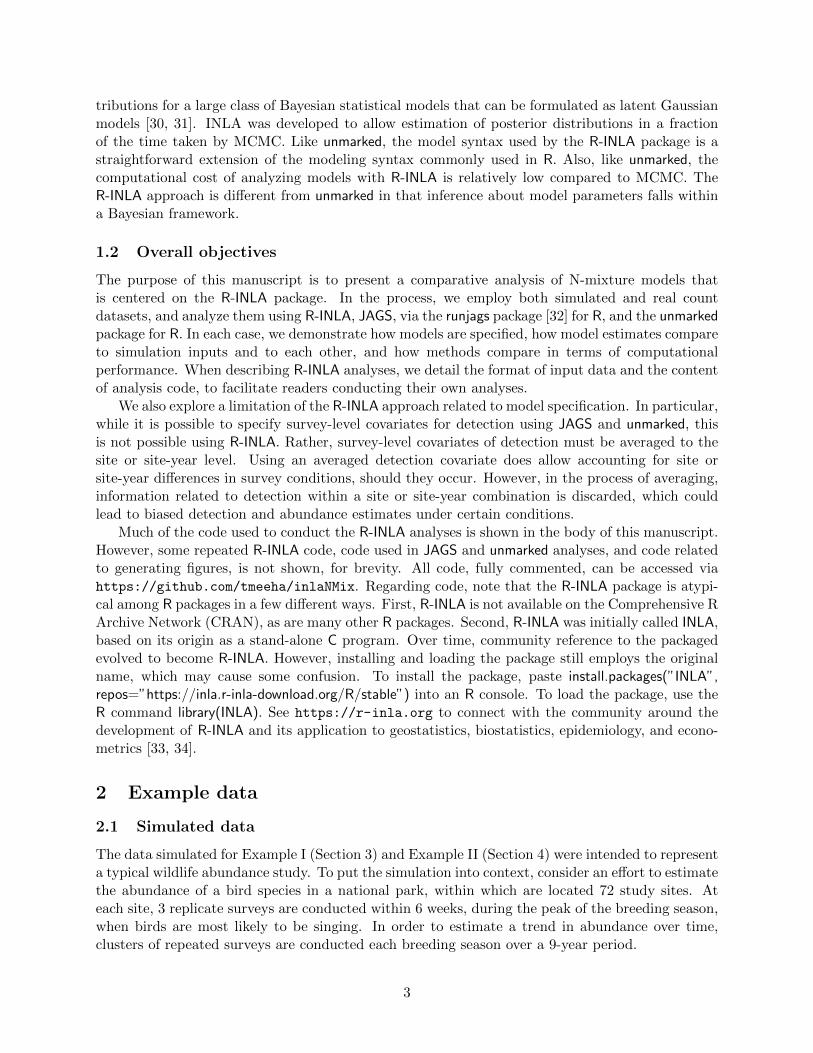
Estimating Animal Abundance with N-Mixture Models Using the

R-INLA Package for R

Timothy D. Meehan, Nicole L. MichelNational Audubon Society

and Havard RueKing Abdulla University of Science and Technology

August 17, 2018

Successful management of wildlife populations requires accurate estimates of abun-dance. Abundance estimates can be confounded by imperfect detection during wildlifesurveys. N-mixture models enable quantification of detection probability and, underappropriate conditions, produce abundance estimates that are less biased. Here, wedemonstrate use of the R-INLA package for R to analyze N-mixture models and com-pare performance of R-INLA to two other common approaches: JAGS (via the runjagspackage for R), which uses Markov chain Monte Carlo and allows Bayesian inference,and the unmarked package for R, which uses maximum likelihood and allows frequentistinference. We show that R-INLA is an attractive option for analyzing N-mixture modelswhen (i) fast computing times are necessary (R-INLA is 10 times faster than unmarkedand 500 times faster than JAGS), (ii) familiar model syntax and data format (relative toother R packages) is desired, (iii) survey-level covariates of detection are not essential,and (iv) Bayesian inference is preferred.

1 Introduction

1.1 Background

Successful management of wildlife species requires accurate estimates of abundance [1]. One com-mon method for estimating animal abundance is direct counts [2]. Efforts to obtain accurate abun-dance estimates via direct counts can be hindered by the cryptic nature of many wildlife species,and by other factors such as observer expertise, weather, and habitat structure [3]. The lack ofperfect detection in wildlife surveys is common, and can cause abundance to be underestimated [4].

In recent years, new survey designs and modeling approaches have enabled improved estimatesof animal abundance that are less biased by imperfect detection [3]. One such survey design,termed a metapopulation design [5], involves repeat visits in rapid succession to each of multiplestudy sites in a study area. If, during repeat visits, the population is assumed to be closed (noimmigration, emigration, reproduction or mortality; i.e., static abundance), then information ondetections and non-detections during repeated counts can inform an estimate of detection probabil-ity. This detection probability can be used to correct abundance estimates for imperfect detection[6].

1

arX

iv:1

705.

0158

1v2

[st

at.A

P] 1

5 A

ug 2

018

Data resulting from this survey design are often modeled using an explicitly hierarchical sta-tistical model referred to in the quantitative wildlife ecology literature as an N-mixture model[7, 8, 6, 9]. One form of an N-mixture model, a binomial mixture model, describes individualobserved counts y at site i during survey j as coming from a binomial distribution with parametersfor abundance N and detection probability p, where N per site is drawn from a Poisson distributionwith an expected value λi. Specifically,

Ni ∼ Pois(λi) and yi,j |Ni ∼ Bin(Ni, pi,j).

λ is commonly modeled as a log-linear function of site covariates, as log(λi) = β0 + β1xi.Similarly, p is commonly modeled as logit(pi,j) = α0 + α1xi,j , a logit-linear function of site-surveycovariates.

This estimation approach can be extended to cover K distinct breeding or wintering seasons,which correspond with distinct years for wildlife species that are resident during annual breedingor wintering stages [10]. In this case, population closure is assumed across J surveys within yeark, but is relaxed across years [10]. A simple specification of a multiple-year model is Ni,k ∼Pois(λi,k), yi,j,k|Ni,k ∼ Bin(Ni,k, pi,j,k). Like the single-year specification, λ is commonly modeledusing site and site-year covariates, and p using site-survey-year covariates.

There are other variations of N-mixture models that accommodate overdispersed counts throughuse of a negative binomial distribution [5], a zero-inflated Poisson distribution [11], or survey-levelrandom effects [12], or underdispersed counts using mixtures of binomial and Conway-Maxwell-Poisson distributions [13]. Yet other variations account for non-independent detection probabilitiesthrough use of a beta-binomial distribution [14], parse different components of detection throughthe use of unique covariates [15], or relax assumptions of population closure [16, 17]. We do notdiscuss all of these variations here, but refer interested readers to [3] for an overview, and to [18]for a discussion of assumptions and limitations.

The development of metapopulation designs and N-mixture models represents a significantadvance in quantitative wildlife ecology. However, there are practical issues that sometimes actas barriers to adoption. Many of the examples of N-mixture models in the wildlife literaturehave employed Bayesian modeling software such as WinBUGS, OpenBUGS, JAGS, or Stan [19, 20,21]. These are extremely powerful and flexible platforms for analyzing hierarchical models, butthey come with a few important challenges. First, many wildlife biologists are not accustomedto coding statistical models using the BUGS or Stan modeling syntax. While there are severaloutstanding resources aimed at teaching these skills [22, 23, 12, 24, 25] learning them is, nonetheless,a considerable commitment. Second, while Markov chain Monte Carlo (MCMC) chains convergequickly for relatively simple N-mixture models, convergence for more complex models can takehours to days, or may not occur at all [12].

There are other tools available for analyzing N-mixture models that alleviate some of thesepractical issues. The unmarked package [26] for R statistical computing software [27] offers severaloptions for analyzing N-mixture models within a maximum likelihood (ML) framework, with thecapacity to accommodate overdispersed counts and dynamic populations. The model coding syntaxused in unmarked is a simple extension of the standard R modeling syntax. Models are analyzedusing ML, so model analysis is often completed in a fraction of the time taken using MCMC. Thefamiliar model syntax and rapid model evaluation of unmarked has undoubtedly contributed to thebroader adoption of N-mixture models by wildlife biologists. However, it comes at a cost, loss ofthe intuitive inferential framework associated with Bayesian analysis.

Here we demonstrate analysis of N-mixture models using the R-INLA package [28, 29] for R.The R-INLA package uses integrated nested Laplace approximation (INLA) to derive posterior dis-

2

tributions for a large class of Bayesian statistical models that can be formulated as latent Gaussianmodels [30, 31]. INLA was developed to allow estimation of posterior distributions in a fractionof the time taken by MCMC. Like unmarked, the model syntax used by the R-INLA package is astraightforward extension of the modeling syntax commonly used in R. Also, like unmarked, thecomputational cost of analyzing models with R-INLA is relatively low compared to MCMC. TheR-INLA approach is different from unmarked in that inference about model parameters falls withina Bayesian framework.

1.2 Overall objectives

The purpose of this manuscript is to present a comparative analysis of N-mixture models thatis centered on the R-INLA package. In the process, we employ both simulated and real countdatasets, and analyze them using R-INLA, JAGS, via the runjags package [32] for R, and the unmarkedpackage for R. In each case, we demonstrate how models are specified, how model estimates compareto simulation inputs and to each other, and how methods compare in terms of computationalperformance. When describing R-INLA analyses, we detail the format of input data and the contentof analysis code, to facilitate readers conducting their own analyses.

We also explore a limitation of the R-INLA approach related to model specification. In particular,while it is possible to specify survey-level covariates for detection using JAGS and unmarked, thisis not possible using R-INLA. Rather, survey-level covariates of detection must be averaged to thesite or site-year level. Using an averaged detection covariate does allow accounting for site orsite-year differences in survey conditions, should they occur. However, in the process of averaging,information related to detection within a site or site-year combination is discarded, which couldlead to biased detection and abundance estimates under certain conditions.

Much of the code used to conduct the R-INLA analyses is shown in the body of this manuscript.However, some repeated R-INLA code, code used in JAGS and unmarked analyses, and code relatedto generating figures, is not shown, for brevity. All code, fully commented, can be accessed viahttps://github.com/tmeeha/inlaNMix. Regarding code, note that the R-INLA package is atypi-cal among R packages in a few different ways. First, R-INLA is not available on the Comprehensive RArchive Network (CRAN), as are many other R packages. Second, R-INLA was initially called INLA,based on its origin as a stand-alone C program. Over time, community reference to the packagedevolved to become R-INLA. However, installing and loading the package still employs the originalname, which may cause some confusion. To install the package, paste install.packages(”INLA”,repos=”https://inla.r-inla-download.org/R/stable”) into an R console. To load the package, use theR command library(INLA). See https://r-inla.org to connect with the community around thedevelopment of R-INLA and its application to geostatistics, biostatistics, epidemiology, and econo-metrics [33, 34].

2 Example data

2.1 Simulated data

The data simulated for Example I (Section 3) and Example II (Section 4) were intended to representa typical wildlife abundance study. To put the simulation into context, consider an effort to estimatethe abundance of a bird species in a national park, within which are located 72 study sites. Ateach site, 3 replicate surveys are conducted within 6 weeks, during the peak of the breeding season,when birds are most likely to be singing. In order to estimate a trend in abundance over time,clusters of repeated surveys are conducted each breeding season over a 9-year period.

3

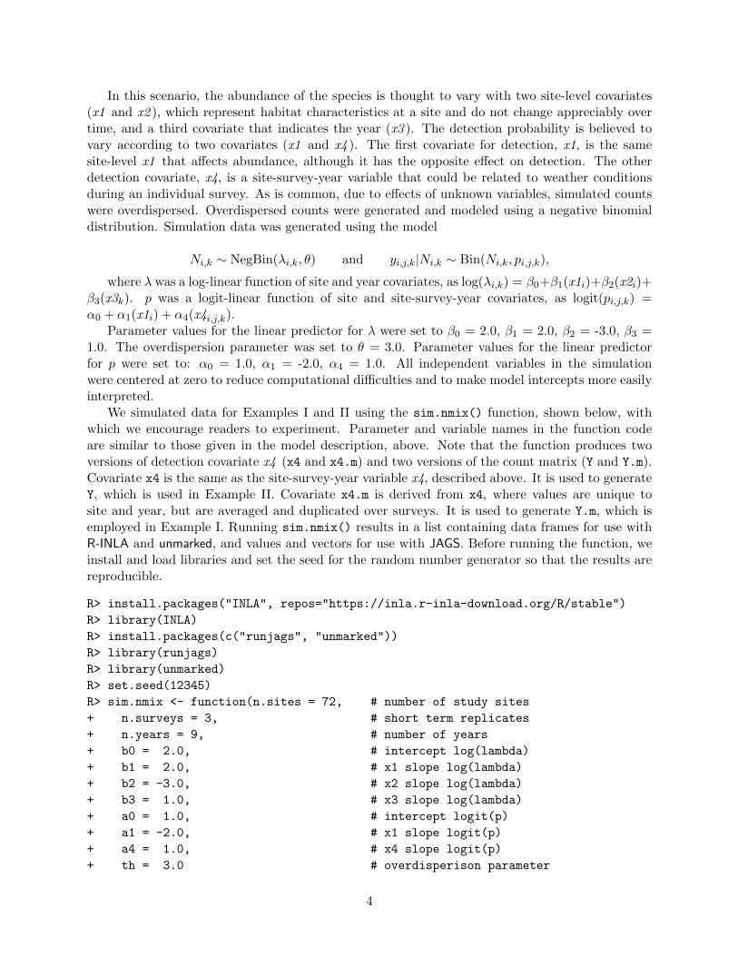
In this scenario, the abundance of the species is thought to vary with two site-level covariates(x1 and x2 ), which represent habitat characteristics at a site and do not change appreciably overtime, and a third covariate that indicates the year (x3 ). The detection probability is believed tovary according to two covariates (x1 and x4 ). The first covariate for detection, x1, is the samesite-level x1 that affects abundance, although it has the opposite effect on detection. The otherdetection covariate, x4, is a site-survey-year variable that could be related to weather conditionsduring an individual survey. As is common, due to effects of unknown variables, simulated countswere overdispersed. Overdispersed counts were generated and modeled using a negative binomialdistribution. Simulation data was generated using the model

Ni,k ∼ NegBin(λi,k, θ) and yi,j,k|Ni,k ∼ Bin(Ni,k, pi,j,k),

where λ was a log-linear function of site and year covariates, as log(λi,k) = β0+β1(x1i)+β2(x2i)+β3(x3k). p was a logit-linear function of site and site-survey-year covariates, as logit(pi,j,k) =α0 + α1(x1i) + α4(x4i,j,k).

Parameter values for the linear predictor for λ were set to β0 = 2.0, β1 = 2.0, β2 = -3.0, β3 =1.0. The overdispersion parameter was set to θ = 3.0. Parameter values for the linear predictorfor p were set to: α0 = 1.0, α1 = -2.0, α4 = 1.0. All independent variables in the simulationwere centered at zero to reduce computational difficulties and to make model intercepts more easilyinterpreted.

We simulated data for Examples I and II using the sim.nmix() function, shown below, withwhich we encourage readers to experiment. Parameter and variable names in the function codeare similar to those given in the model description, above. Note that the function produces twoversions of detection covariate x4 (x4 and x4.m) and two versions of the count matrix (Y and Y.m).Covariate x4 is the same as the site-survey-year variable x4, described above. It is used to generateY, which is used in Example II. Covariate x4.m is derived from x4, where values are unique tosite and year, but are averaged and duplicated over surveys. It is used to generate Y.m, which isemployed in Example I. Running sim.nmix() results in a list containing data frames for use withR-INLA and unmarked, and values and vectors for use with JAGS. Before running the function, weinstall and load libraries and set the seed for the random number generator so that the results arereproducible.

R> install.packages("INLA", repos="https://inla.r-inla-download.org/R/stable")

R> library(INLA)

R> install.packages(c("runjags", "unmarked"))

R> library(runjags)

R> library(unmarked)

R> set.seed(12345)

R> sim.nmix <- function(n.sites = 72, # number of study sites

+ n.surveys = 3, # short term replicates

+ n.years = 9, # number of years

+ b0 = 2.0, # intercept log(lambda)

+ b1 = 2.0, # x1 slope log(lambda)

+ b2 = -3.0, # x2 slope log(lambda)

+ b3 = 1.0, # x3 slope log(lambda)

+ a0 = 1.0, # intercept logit(p)

+ a1 = -2.0, # x1 slope logit(p)

+ a4 = 1.0, # x4 slope logit(p)

+ th = 3.0 # overdisperison parameter

4

+ ){

+

+ # make empty N and Y arrays

+ if(n.years %% 2 == 0) {n.years <- n.years + 1}

+ N.tr <- array(dim = c(n.sites, n.years))

+ Y <- array(dim = c(n.sites, n.surveys, n.years))

+ Y.m <- array(dim = c(n.sites, n.surveys, n.years))

+

+ # create abundance covariate values

+ x1 <- array(as.numeric(scale(runif(n = n.sites, -0.5, 0.5), scale = F)),

+ dim = c(n.sites, n.years))

+ x2 <- array(as.numeric(scale(runif(n = n.sites, -0.5, 0.5), scale = F)),

+ dim = c(n.sites, n.years))

+ yrs <- 1:n.years; yrs <- (yrs - mean(yrs)) / (max(yrs - mean(yrs))) / 2

+ x3 <- array(rep(yrs, each = n.sites), dim = c(n.sites, n.years))

+

+ # fill true N array

+ lam.tr <- exp(b0 + b1 * x1 + b2 * x2 + b3 * x3)

+ for(i in 1:n.sites){

+ for(k in 1:n.years){

+ N.tr[i, k] <- rnbinom(n = 1, mu = lam.tr[i, k], size = th)

+ }}

+

+ # create detection covariate values

+ x1.p <- array(x1[,1], dim = c(n.sites, n.surveys, n.years))

+ x4 <- array(as.numeric(scale(runif(n = n.sites * n.surveys * n.years,

+ -0.5, 0.5), scale = F)), dim = c(n.sites, n.surveys, n.years))

+

+ # average x4 per site-year for example 1

+ x4.m <- apply(x4, c(1, 3), mean, na.rm = F)

+ out1 <- c()

+ for(k in 1:n.years){

+ chunk1 <- x4.m[ , k]

+ chunk2 <- rep(chunk1, n.surveys)

+ out1 <- c(out1, chunk2)

+ }

+ x4.m.arr <- array(out1, dim = c(n.sites, n.surveys, n.years))

+

+ # fill Y.m count array using x4.m for example 1

+ p.tr1 <- plogis(a0 + a1 * x1.p + a4 * x4.m.arr)

+ for (i in 1:n.sites){

+ for (k in 1:n.years){

+ for (j in 1:n.surveys){

+ Y.m[i, j, k] <- rbinom(1, size = N.tr[i, k], prob = p.tr1[i, j, k])

+ }}}

+

+ # fill Y count array using x4 for example 2

+ p.tr2 <- plogis(a0 + a1 * x1.p + a4 * x4)

5

+ for (i in 1:n.sites){

+ for (k in 1:n.years){

+ for (j in 1:n.surveys){

+ Y[i, j, k] <- rbinom(1, size = N.tr[i, k], prob = p.tr2[i, j, k])

+ }}}

+

+ # format Y.m for data frame output for inla and unmarked

+ Y.m.df <- Y.m[ , , 1]

+ for(i in 2:n.years){

+ y.chunk <- Y.m[ , , i]

+ Y.m.df <- rbind(Y.m.df, y.chunk)

+ }

+

+ # format covariates for data frame output for inla and unmarked

+ x1.df <- rep(x1[ , 1], n.years)

+ x2.df <- rep(x2[ , 1], n.years)

+ x3.df <- rep(x3[1, ], each = n.sites)

+ x1.p.df <- rep(x1.p[ , 1, 1], n.years)

+ x4.df <- c(x4.m)

+

+ # put together data frames for inla and unmarked

+ inla.df <- unmk.df <- data.frame(y1 = Y.m.df[ , 1], y2 = Y.m.df[ , 2],

+ y3 = Y.m.df[ , 3], x1 = x1.df, x2 = x2.df, x3 = x3.df,

+ x1.p = x1.p.df, x4.m = x4.df)

+

+ # return all necessary data for examples 1 and 2

+ return(list(inla.df = inla.df, unmk.df = unmk.df, n.sites = n.sites,

+ n.surveys = n.surveys, n.years = n.years, x1 = x1[ , 1],

+ x2 = x2[ , 1], x3 = x3[1, ], x4 = x4, x4.m = x4.m, x4.m.arr = x4.m.arr,

+ Y = Y, Y.m = Y.m, lam.tr = lam.tr, N.tr = N.tr, x1.p = x1.p[ , 1, 1]

+ ))

+

+ } # end sim.nmix function

R> sim.data <- sim.nmix()

2.2 Real data

In addition to simulated data, we also demonstrate the use of R-INLA and unmarked with a realdataset in Example III in Section 5. This dataset comes from a study by [9] and is publiclyavailable as part of the unmarked package. The dataset includes mallard duck (Anas platyrhynchos)counts, conducted at 239 sites on 2 or 3 occasions during the summer of 2002, as part of a Swissprogram that monitors breeding bird abundance (Monitoring Haufige Brutvogel or Swiss BreedingBird Survey). In addition to counts, the dataset also includes 2 site-survey covariates related todetection (survey effort and survey date), and 3 site-level covariates related to abundance (routelength, route elevation, and forest cover). Full dataset details are given in [9].

6

3 Example I

3.1 Goals

In Example I, we demonstrate the use of R-INLA and compare use and performance to similaranalyses using JAGS and unmarked. In this first example, the functional forms of R-INLA, JAGS,and unmarked models match the data generating process. Specifically, we used the covariate x4.m

to generate the count matrix Y.m, and analyzed the data with models that use x4.m as a covariate.This example was intended to demonstrate the differences and similarities in use, computationtime, and estimation results across the three methods when the specified models were the same asthe data generating process.

3.2 Analysis with R-INLA

We first analyze the simulated data using the R-INLA package. The list returned from the sim.nmix()function includes an object called inla.df. This object has the following structure.

R> str(sim.data$inla.df, digits.d = 2)

’data.frame’: 648 obs. of 8 variables:

$ y1 : int 2 12 25 3 0 3 1 7 2 8 ...

$ y2 : int 2 22 25 4 1 3 1 11 2 4 ...

$ y3 : int 4 11 28 2 1 2 0 10 2 3 ...

$ x1 : num 0.198 0.353 0.238 0.364 -0.066 ...

$ x2 : num -0.159 -0.197 -0.484 0.087 0.429 ...

$ x3 : num -0.5 -0.5 -0.5 -0.5 -0.5 -0.5 -0.5 ...

$ x1.p : num 0.198 0.353 0.238 0.364 -0.066 ...

$ x4.m : num 0.148 -0.07 0.206 -0.261 -0.046 ...

R> round(head(sim.data$inla.df), 3)

y1 y2 y3 x1 x2 x3 x1.p x4.m

1 2 2 4 0.198 -0.159 -0.5 0.198 0.148

2 12 22 11 0.353 -0.197 -0.5 0.353 -0.070

3 25 25 28 0.238 -0.484 -0.5 0.238 0.206

4 3 4 2 0.364 0.087 -0.5 0.364 -0.261

5 0 1 1 -0.066 0.429 -0.5 -0.066 -0.046

6 3 3 2 -0.356 0.123 -0.5 -0.356 -0.036

This data frame representation of the simulated data has 72 sites × 9 years = 648 rows. Hadthere only been one year of data, then the data frame would have 72 rows, one per site. The dataframe has three columns (y1, y2, and y3) with count data from the count matrix Y.m, one foreach of the three replicate surveys within a given year. Had there been six surveys per year, thenthere would have been six count columns. The three variables thought to affect abundance arerepresented in columns 4 through 6. Note that, in this scenario, the first two abundance variablesare static across years, so there are 72 unique values in a vector that is stacked 9 times. The thirdabundance variable, the indicator for year, is a sequence of 9 values, where each value is repeated72 times. It is centered and scaled in this example. The two variables thought to affect detectionprobability are represented in columns 7 and 8. The first of these variables has the same values asin column 4, so column 7 is a simple copy of column 4. The second of the two detection variables,

7

shown in column 8, varies per site and year in Example I, so there are 648 unique values in thiscolumn. Note that any of the covariates for abundance or detection could have varied by site andyear, like x4.m.

We made small modifications to this data frame to prepare data for analysis with R-INLA. In thecode that follows, we use the inla.mdata() function to create an object called counts.and.count.covs.The counts.and.count.covs object is essentially a bundle of information related to the abundancecomponent of the model. Calling the str() function shows that this object is an R-INLA list thatincludes the three count vectors, passed to the function as a matrix, one vector containing the valueof 1, which specifies a global intercept for λ, and three vectors corresponding to the covariates forλ. Note that the variable names are standardized by inla.mdata() for computational reasons.

R> inla.data <- sim.data$inla.df

R> y.mat <- as.matrix(inla.data[,c("y1", "y2", "y3")])

R> counts.and.count.covs <- inla.mdata(y.mat, 1, inla.data$x1,

+ inla.data$x2, inla.data$x3)

R> str(counts.and.count.covs)

List of 7

$ Y1: int [1:648] 2 12 25 3 0 3 1 7 2 8 ...

$ Y2: int [1:648] 2 22 25 4 1 3 1 11 2 4 ...

$ Y3: int [1:648] 4 11 28 2 1 2 0 10 2 3 ...

$ X1: num [1:648] 1 1 1 1 1 1 1 1 1 1 ...

$ X2: num [1:648] 0.1983 0.3532 0.2384 0.3636 -0.0661 ...

$ X3: num [1:648] -0.1595 -0.1966 -0.4842 0.0865 0.429 ...

$ X4: num [1:648] -0.5 -0.5 -0.5 -0.5 -0.5 -0.5 -0.5 -0.5 -0.5 -0.5 ...

- attr(*, "class")= chr "inla.mdata"

Analysis of N-mixture models with R-INLA is accomplished with a call to the inla() function.The first argument in the inla() call, shown below, is the model formula. On the left side of theformula is the counts.and.count.covs object, which includes the vectors of counts, the globalintercept for λ, and the covariates related to λ. On the right side of the formula is a 1, to specifya global intercept for p, and the two covariates for p. Note that a wide range of random effects(exchangeable, spatially or temporally structured) for p could be added to the right side of theformula using the f() syntax [29].

The second argument to inla() describes the data, provided here as a list that corresponds withthe model formula. Third is the likelihood family, which can take values of "nmix" for a Poisson-binomial mixture and "nmixnb" for a negative binomial-binomial mixture. Run the commandinla.doc("nmix") for more information on these likelihood families. The fourth (control.fixed,for detection parameters) and fifth (control.family, for abundance and overdispersion param-eters) arguments specify the priors for the two model components. Here, the priors for bothabundance and detection parameters are vague normal distributions centered at zero with preci-sion equal to 0.01. The prior for the overdispersion parameter is specified as uniform. Note thata wide variety of other prior distributions are available in R-INLA. At the end of the call are argu-ments to print the progress of model fitting, and to save information that will enable computationof fitted values. Several other characteristics of the analysis can be modified in a call to inla(),such as whether or not deviance information criterion (DIC), widely applicable information crite-rion (WAIC), conditional predictive ordinate (CPO), or probability integral transform (PIT) arecomputed. See [29] for details.

8

R> out.inla.1 <- inla(counts.and.count.covs ~ 1 + x1.p + x4.m,

+ data = list(counts.and.count.covs = counts.and.count.covs,

+ x1.p = inla.data$x1.p, x4.m = inla.data$x4.m),

+ family = "nmixnb",

+ control.fixed = list(mean = 0, mean.intercept = 0, prec = 0.01,

+ prec.intercept = 0.01),

+ control.family = list(hyper = list(theta1 = list(param = c(0, 0.01)),

+ theta2 = list(param = c(0, 0.01)), theta3 = list(param = c(0, 0.01)),

+ theta4 = list(param = c(0, 0.01)), theta5 = list(prior = "flat",

+ param = numeric()))),

+ verbose = TRUE,

+ control.compute=list(config = TRUE))

R> summary(out.inla.1, digits = 3)

Time used (seconds):

Pre-processing Running inla Post-processing Total

0.421 5.081 0.342 5.844

Fixed effects:

mean sd 0.025quant 0.5quant 0.975quant

(Intercept) 1.053 0.058 0.938 1.054 1.165

x1.p -1.996 0.197 -2.385 -1.995 -1.611

x4.m 1.056 0.313 0.440 1.056 1.668

Model hyperparameters:

mean sd 0.025quant 0.5quant 0.975quant

beta[1] 2.022 0.034 1.956 2.022 2.090

beta[2] 2.070 0.116 1.839 2.071 2.295

beta[3] -2.951 0.099 -3.142 -2.953 -2.755

beta[4] 1.142 0.088 0.969 1.142 1.316

overdisp 0.349 0.028 0.296 0.349 0.407

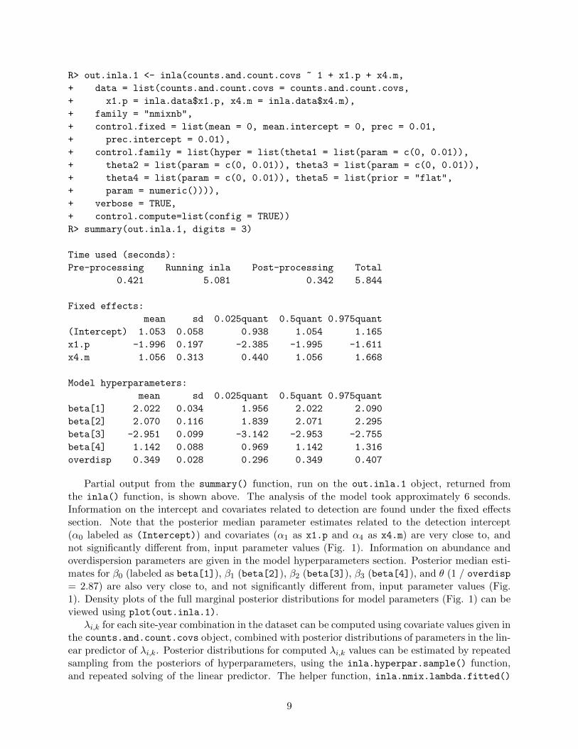
Partial output from the summary() function, run on the out.inla.1 object, returned fromthe inla() function, is shown above. The analysis of the model took approximately 6 seconds.Information on the intercept and covariates related to detection are found under the fixed effectssection. Note that the posterior median parameter estimates related to the detection intercept(α0 labeled as (Intercept)) and covariates (α1 as x1.p and α4 as x4.m) are very close to, andnot significantly different from, input parameter values (Fig. 1). Information on abundance andoverdispersion parameters are given in the model hyperparameters section. Posterior median esti-mates for β0 (labeled as beta[1]), β1 (beta[2]), β2 (beta[3]), β3 (beta[4]), and θ (1 / overdisp

= 2.87) are also very close to, and not significantly different from, input parameter values (Fig.1). Density plots of the full marginal posterior distributions for model parameters (Fig. 1) can beviewed using plot(out.inla.1).

λi,k for each site-year combination in the dataset can be computed using covariate values given inthe counts.and.count.covs object, combined with posterior distributions of parameters in the lin-ear predictor of λi,k. Posterior distributions for computed λi,k values can be estimated by repeatedsampling from the posteriors of hyperparameters, using the inla.hyperpar.sample() function,and repeated solving of the linear predictor. The helper function, inla.nmix.lambda.fitted()

9

produces fitted lambda values as described, using the information contained in the model resultoutput. A call to this function, specifying the model result, estimated posterior sample size, andsummary output, is as follows.

R> out.inla.1.lambda.fits <- inla.nmix.lambda.fitted(result = out.inla.1,

+ sample.size = 5000, return.posteriors = F)$fitted.summary

R> head(out.inla.1.lambda.fits)

index mean.lambda sd.lambda q025.lambda median.lambda q975.lambda

1 1 10.3329 0.6623 9.0980 10.3109 11.6683

2 2 15.9003 1.1895 13.6760 15.8649 18.3523

3 3 29.2742 2.2882 25.0410 29.2043 34.0370

4 4 7.0490 0.5250 6.0663 7.0270 8.1227

5 5 1.0547 0.0810 0.9072 1.0509 1.2194

6 6 1.4272 0.1031 1.2389 1.4255 1.6353

The output from this function call is a summary of estimated posteriors for fitted λi,k values.In this example, there are 648 rows. Comparisons of posterior median fitted λi,k with simulatedλi,k and Ni,k values are shown below.

R> summary(out.inla.1.lambda.fits$median.lambda)

Min. 1st Qu. Median Mean 3rd Qu. Max.

0.6538 3.4020 7.0070 13.5200 16.0300 123.2000

R> summary(c(sim.data$lam.tr))

Min. 1st Qu. Median Mean 3rd Qu. Max.

0.6834 3.3050 6.8190 13.0300 15.9500 111.3000

R> cor(out.inla.1.lambda.fits$median.lambda, c(sim.data$lam.tr))

[1] 0.9986

R> sum(out.inla.1.lambda.fits$median.lambda)

[1] 8758.542

R> sum(c(sim.data$lam.tr))

[1] 8444.975

R> sum(c(sim.data$N.tr))

[1] 8960

3.3 Analysis with JAGS

Next, we analyzed the same simulated dataset using JAGS, via the runjags package. As for theR-INLA analysis, we specified a negative binomial distribution for abundance, vague normal priorsfor the intercepts and the global effects of the covariates of λ and p, and a flat prior for theoverdispersion parameter. The JAGS model statement, where the distributions and likelihoodfunction are specified, is shown below for comparison with the arguments to inla().

10

Figure 1: Marginal posteriors of model parameters from R-INLA (dashed black lines) and JAGS(solid gray lines), along with Maximum Liklihood estimates (black circles) and 95% confidenceintervals (horizontal black lines) from unmarked. True input values are represented by verticalblack lines.

11

R> jags.model.string <- "

+ model {

+ a0 ~ dnorm(0, 0.01)

+ a1 ~ dnorm(0, 0.01)

+ a4 ~ dnorm(0, 0.01)

+ b0 ~ dnorm(0, 0.01)

+ b1 ~ dnorm(0, 0.01)

+ b2 ~ dnorm(0, 0.01)

+ b3 ~ dnorm(0, 0.01)

+ th ~ dunif(0, 5)

+ for (k in 1:n.years){

+ for (i in 1:n.sites){

+ N[i, k] ~ dnegbin(prob[i, k], th)

+ prob[i, k] <- th / (th + lambda[i, k])

+ log(lambda[i, k]) <- b0 + (b1 * x1[i]) + (b2 * x2[i]) + (b3 * x3[k])

+ for (j in 1:n.surveys){

+ Y.m[i, j, k] ~ dbin(p[i,j,k], N[i,k])

+ p[i, j, k] <- exp(lp[i,j,k]) / (1 + exp(lp[i,j,k]))

+ lp[i, j, k] <- a0 + (a1 * x1.p[i]) + (a4 * x4.m[i, k])

+ }}}}

+ "

After specifying the JAGS model, we define the parameters to be monitored during the MCMCsimulations, bundle numerous values and vectors from the sim.data object, and create a functionfor drawing random initial values for the model parameters. These steps are included in the codesupplement, but are not shown here. Finally, we set the run parameters, such as the number ofchains and iterations, and start the MCMC process. Run parameters were chosen such that MCMCdiagnostics indicated converged chains (potential scale reduction factors ≤ 1.05) and reasonablyrobust posterior distributions (effective sample sizes ≥ 3000). Note that the recommended numberof effective samples for particularly robust inference is closer to 6000 [35]. Thus, MCMC processingtimes reported here could be considered optimistic estimates. The MCMC simulation is initiatedwith a call to run.jags(). Partial output from the simulation, related to parameter estimates, isshown below.

R> out.jags.1 <- run.jags(model = jags.model.string, data = jags.data,

+ monitor = params, n.chains = 3, inits = inits, burnin = 3000,

+ adapt = 3000, sample = 6000, thin = 10, modules = "glm on",

+ method = "parallel")

R> round(summary(out.jags.1), 3)[ , c(1:5, 9, 11)]

Lower95 Median Upper95 Mean SD SSeff psrf

a0 0.941 1.053 1.161 1.053 0.057 3155 1

a1 -2.380 -1.990 -1.618 -1.994 0.195 2954 1

a4 0.434 1.053 1.661 1.052 0.314 5695 1

b0 1.956 2.024 2.089 2.024 0.034 7065 1

b1 1.851 2.070 2.301 2.071 0.115 6028 1

b2 -3.142 -2.946 -2.755 -2.947 0.099 17539 1

b3 0.969 1.142 1.315 1.142 0.089 18000 1

12

th 2.401 2.840 3.295 2.850 0.230 18000 1

Similar to the R-INLA analysis, median parameter estimates from the JAGS model were closeto, and not significantly different from, the input values used to generate the data (Fig. 1). Thepotential scale reduction factor for all variables was ≥ 1.05, and the effective sample size for allvariables was approximately 3000 or greater. The simulation ran in parallel on 3 virtual cores, 1MCMC chain per core, and took approximately 2960 seconds.

3.4 Analysis with unmarked

Lastly, we prepare the simulated data for the unmarked analysis, which involved slight modificationof the unmk.df object created using the sim.nmix() function. As with the JAGS analysis, thesesteps are included in the code supplement, but are not illustrated here.

The unmarked analysis is run by a call to the pcount() function. The first argument in thecall to pcount() is the model formula, which specifies the covariates for detection, and then thecovariates for abundance. This is followed by an argument identifying the unmarked data object,and the form of the mixture model, negative binomial-binomial in this case.

R> out.unmk.1 <- pcount(~ 1 + x1.p + x4.m ~ 1 + x1 + x2 + x3,

+ data = unmk.data, mixture = "NB")

R> summary(out.unmk.1)

Abundance (log-scale):

Estimate SE z P(>|z|)

(Intercept) 2.02 0.0321 62.9 0.00e+00

x1 2.04 0.1071 19.0 1.69e-80

x2 -2.94 0.0982 -29.9 5.36e-20

x3 1.14 0.0882 13.0 2.26e-38

Detection (logit-scale):

Estimate SE z P(>|z|)

(Intercept) 1.08 0.0507 21.27 2.29e-100

x1.p -1.90 0.1576 -12.08 1.30e-33

x4.m 1.04 0.3102 3.35 8.02e-04

Dispersion (log-scale):

Estimate SE z P(>|z|)

1.05 0.0804 13.1 4.91e-39

Maximum likelihood estimates for model parameters from unmarked were also close to, andnot significantly different from, input values (Fig. 1). Note that the dispersion estimate, afterexponentiation, was 2.86. The unmarked estimates were produced in approximately 86 seconds.

3.5 Example I summary

Example I demonstrated basic use of R-INLA to analyze N-mixture models and highlighted sim-ilarities and differences between it and two other commonly used approaches. In demonstratingthe use of R-INLA, we showed that the input data format is not too complicated, and that theformatting process can be accomplished with a few lines of code. Similarly, model specification

13

uses a straightforward extension of the standard syntax in R, where the counts and covariates for λare specified through an R-INLA object included on the left side of the formula, and fixed covariatesand random effects for p are specified on the right side of the formula. The data format and modelspecification syntax of R-INLA is not too different from unmarked, whereas those of both packagesare considerably different from JAGS and other MCMC software, such as OpenBUGS, WinBUGS,and Stan.

Regarding performance, R-INLA, JAGS, and unmarked all successfully extracted simulation in-put values. Fig. 1 shows marginal posterior distributions produced by R-INLA and JAGS, andestimates and 95% confidence intervals from unmarked. These results derive from data from onerandom manifestation of the input values. Thus, we do not expect the posterior distributions forthe estimates to be centered at the input values, which would be expected if the simulation wasrepeated many times. However, we do expect the input values to fall somewhere within the pos-terior distributions and 95% confidence limits, which is what occured here. Fig. 1 shows that,for similarly specified models, R-INLA (dashed black lines) and JAGS (solid gray lines) yieldedpractically identical marginal posterior distributions for model parameters. Fig. 1 also illustratesthe general agreement between the credible intervals associated with R-INLA and JAGS and theconfidence intervals associated with unmarked.

Where R-INLA, JAGS, and unmarked differed substantially was in computing time. In thisexample, R-INLA took 6 seconds, JAGS took 2960 seconds, and unmarked took 86 seconds to produceresults. Thus, R-INLA was approximately 500 times faster than JAGS and 10 times faster thanunmarked. This was the case despite the fact that unmarked produced ML estimates and the JAGSanalysis was run in parallel with each of three MCMC chains simulated on a separate virtualcomputing core. If parallel computing had not been used with JAGS, processing the JAGS modelwould have taken approximately twice as long. If MCMC simulations were run until effective samplesizes of 6000 were reached, processing time would have doubled again.

In sum, when compared to other tools, R-INLA is relatively easy to implement and producesaccurate estimates of Bayesian posteriors very quickly. Its utility depends on the degree to which thedata generating process can be captured accurately in model specification. However, as mentionedabove, certain N-mixture models can not be specified using R-INLA. For the data in Example I,the count matrix was produced using a detection covariate that was averaged to the site-year level.This averaged covariate was subsequently specified in the model. But what happens when thesite-survey-year covariate is an important component of the data generating process, and it can’tbe entered into the model in this form? This is the question explored in Example II.

4 Example II

4.1 Goals

In Example II, we show the consequences of not being able to specify a site-survey-year covariatefor detection, under a range of conditions. We conducted a Monte Carlo experiment where, for eachiteration, the count matrix for the analysis, Y, was generated with the sim.nmix() function using thesite-survey-year covariate x4. The count data were then analyzed with two JAGS models. The firstmodel incorporated the site-survey-year x4 covariate. The second model incorporated the averagedsite-year x4.m, instead. For each iteration, we randomly varied the size of α4 when generating thesimulated data. We expected that the simpler model, with x4.m, would yield biased estimates whenthe magnitude of α4 was relatively large, and unbiased estimates when the magnitude of α4 wasrelatively small. All computing code related to Example II is given in the supplemental code file.

14

4.2 Analysis with JAGS

Parameter values entered into sim.nmix(), other than those for α4, were the same as those usedin Example I. Similarly, the JAGS model specification, other than parts associated with α4, wasthe same as that used in Example I. Given the long processing time associated with JAGS modelsin Example I, we only ran and saved 1000 MCMC simulations (no thinning, after 500 adaptiveand 100 burn-in iterations) during each of the 50 Monte Carlo runs in Example II. This numberis not sufficient for drawing inference from marginal posteriors, but was sufficient for looking atqualitative patterns in posterior medians. For each of these runs, a value for α4 was drawn froma uniform distribution that ranged from -3 to 3. Parameter bias was represented for each modelparameter as the difference between the simulation input and the posterior median estimated value.The results of the simulations are depicted in Fig. 2.

4.3 Example II summary

Even with as few as 50 Monte Carlo runs, it was apparent that biases in parameter estimatesincreased with the magnitude of α4 (Fig. 2). When the magnitude of α4 was small, with anabsolute value less than 1, the bias was negligible. When the magnitude of α4 was large, with anabsolute value greater than 2, the bias was considerable (Fig. 2). When interpreting the effect size,bear in mind that x4 ranged from -0.5 to 0.5.

5 Example III

5.1 Goals

In Example III, we explore the performance of R-INLA using real data, a publicly available datasetof mallard duck counts from Switzerland during 2002. By employing real data, we hoped to evaluate(i) the performance of R-INLA using data that were not predictable by design and (ii) the practicalconsequences of not being able to specify site-survey covariates in R-INLA. The dataset is availableas a demonstration dataset in unmarked, so we compared the performance of R-INLA with that ofunmarked, using the analysis settings and model structure described in unmarked documentation.

5.2 Analysis with R-INLA

The mallard data is provided in the unmarked package as a list with three components: a matrixof counts (mallard.y), a list of matrices of detection covariates (mallard.obs), and a data frameof abundance covariates (mallard.site). Data in unmarked are organized in structures calledunmarked frames, which are viewed as a data frame when printed.

R> data(mallard)

R> mallard.umf <- unmarkedFramePCount(y = mallard.y, siteCovs =

+ mallard.site, obsCovs = mallard.obs)

R> mallard.umf[1:6, ]

Data frame representation of unmarkedFrame object.

y1 y2 y3 elev length forest ivel1 ivel2 ivel3

1 0 0 0 -1.173 0.801 -1.156 -0.506 -0.506 -0.506

2 0 0 0 -1.127 0.115 -0.501 -0.934 -0.991 -1.162

3 3 2 1 -0.198 -0.479 -0.101 -1.136 -1.339 -1.610

15

Figure 2: Differences between posterior median parameter values and true input parameter valuesas a function of the α4 value used to simulate data. Black circles and lines are from the model withthe site-survey-year covariate, x4, and gray circles and lines are from the model with an averagedsite-year covariate, x4.m. Parameter name is given in the strip across the top of each panel.

16

4 0 0 0 -0.105 0.315 0.008 -0.819 -0.927 -1.197

5 3 0 3 -1.034 -1.102 -1.193 0.638 0.880 1.042

6 0 0 0 -0.848 0.741 0.917 -1.329 -1.042 -0.899

...

date1 date2 date3

1 -1.761 0.310 1.381

2 -2.904 -1.047 0.596

3 -1.690 -0.476 1.453

4 -2.190 -0.690 1.239

5 -1.833 0.167 1.381

6 -2.619 0.167 1.381

As discussed above, it is not possible to take advantage of survey-level covariates when analyzingN-mixture models with R-INLA. So, before analysis with R-INLA, we averaged the survey-levelvariables, ivel and date, per site using the rowMeans() function.

R> length <- mallard.site[ , "length"]

R> elev <- mallard.site[ , "elev"]

R> forest <- mallard.site[ , "forest"]

R> mean.ivel <- rowMeans(mallard.obs$ivel, na.rm = T)

R> mean.ivel[is.na(mallard.ivel)] <- mean(mallard.ivel, na.rm = T)

R> mean.date <- rowMeans(mallard.obs$date, na.rm = T)

R> mean.date.sq <- mean.date^2

R> mallard.inla.df <- data.frame(y1 = mallard.y[ , "y.1"],

+ y2 = mallard.y[ , "y.2"], y3 = mallard.y[ , "y.3"],

+ length, elev, forest, mean.ivel, mean.date, mean.date.sq)

R> round(head(mallard.inla.df), 3)

y1 y2 y3 length elev forest mean.ivel mean.date mean.date.sq

1 0 0 0 0.801 -1.173 -1.156 -0.506 -0.023 0.001

2 0 0 0 0.115 -1.127 -0.501 -1.029 -1.118 1.251

3 3 2 1 -0.479 -0.198 -0.101 -1.362 -0.238 0.056

4 0 0 0 0.315 -0.105 0.008 -0.981 -0.547 0.299

5 3 0 3 -1.102 -1.034 -1.193 0.853 -0.095 0.009

6 0 0 0 0.741 -0.848 0.917 -1.090 -0.357 0.127

The data are now in a format that can be analyzed readily using R-INLA. The data frame has 239sites × 1 year = 239 rows, one column for each replicate count, and one column for each detectionand abundance covariate. Once in this form, it is easy to create an inla.mdata() object and runthe analysis. In preparing counts.and.count.covs, we specify an intercept and effects of transectlength (length), elevation (elev), and forest cover (forest) on abundance. In the model argumentto inla(), we specify an intercept and effects of survey intensity (ivel) and survey date (date)for detection. As before, the data argument is a list that corresponds with the model formula.The family argument specifies a negative binomial-binomial mixture. The priors for intercepts andcovariates are specified as vague normal distributions, and that for the overdispersion parameteras a uniform distribution.

R> counts.and.count.covs <- inla.mdata(mallard.y, 1, length, elev, forest)

R> out.inla.2 <- inla(counts.and.count.covs ~ 1 + mean.ivel +

17

+ mean.date + mean.date.sq,

+ data = list(counts.and.count.covs = counts.and.count.covs,

+ mean.ivel = mallard.inla.df$mean.ivel, mean.date =

+ mallard.inla.df$mean.date, mean.date.sq = mallard.inla.df$mean.date.sq),

+ family = "nmixnb",

+ control.fixed = list(mean = 0, mean.intercept = 0, prec = 0.01,

+ prec.intercept = 0.01),

+ control.family = list(hyper = list(theta1 = list(param = c(0, 0.01)),

+ theta2 = list(param = c(0, 0.01)), theta3 = list(param = c(0, 0.01)),

+ theta4 = list(param = c(0, 0.01)), theta5 = list(prior = "flat",

+ param = numeric()))))

R> summary(out.inla.2, digits = 3)

A portion of the summary for out.inla.2 is shown below. Note that posterior summariesdescribed in the fixed effects section pertain to the intercept and covariates of p. In the hyperpa-rameters section, beta[1], beta[2], beta[3], and beta[4] identify posterior summaries for the λintercept, and transect length, elevation, and forest cover effects.

Fixed effects:

mean sd 0.025quant 0.5quant 0.975quant

(Intercept) -0.397 0.383 -1.170 -0.389 0.335

mean.ivel 0.039 0.212 -0.378 0.039 0.455

mean.date -1.044 0.433 -1.923 -1.036 -0.195

mean.date.sq -0.318 0.304 -0.962 -0.301 0.233

Model hyperparameters:

mean sd 0.025quant 0.5quant 0.975quant

beta[1] -1.412 0.296 -1.966 -1.424 -0.801

beta[2] -0.290 0.190 -0.664 -0.291 0.086

beta[3] -0.998 0.318 -1.595 -1.011 -0.341

beta[4] -0.771 0.203 -1.178 -0.767 -0.382

overdisp 1.228 0.264 0.799 1.194 1.837

5.3 Analysis with unmarked

The unmarked frame, mallard.umf, created above, can be used directly by the pcount() functionin unmarked. The data and model structure described in the pcount() function below is similarto that used above in the R-INLA analysis, except for one key difference: here, ivel and date aresite-survey level variables instead of the site-level means used in the R-INLA analysis.

R> out.unmk.2 <- pcount(~ ivel+ date + I(date^2) ~ length + elev + forest,

+ mixture = "NB", mallard.umf)

R> summary(out.unmk.2)

Abundance (log-scale):

Estimate SE z P(>|z|)

(Intercept) -1.786 0.281 -6.350 2.15e-10

length -0.186 0.214 -0.868 3.86e-01

elev -1.372 0.293 -4.690 2.73e-06

18

forest -0.685 0.216 -3.166 1.54e-03

Detection (logit-scale):

Estimate SE z P(>|z|)

(Intercept) -0.028 0.285 -0.099 0.921

ivel 0.174 0.227 0.766 0.444

date -0.313 0.147 -2.132 0.033

I(date^2) -0.005 0.081 -0.059 0.953

Dispersion (log-scale):

Estimate SE z P(>|z|)

-0.695 0.364 -1.91 0.056

5.4 Example III summary

Comparing the results, we see that the 95% credible intervals for parameter estimates from theR-INLA analysis overlapped broadly with the 95% confidence intervals from the unmarked analysis,so parameter estimates were not significantly different from one another (Fig. 3). Regardless oftechnique, the same set of parameters had estimates significantly different from zero (Fig. 3), andsignificant effects were of the same magnitude and direction in both analyses. Using both techniques,detection decreased as the season progressed, and abundance decreased with increasing forest coverand elevation. Parameter estimates and biological conclusions were similar despite the fact thatsite-survey detection covariates were used for unmarked and site-averaged detection covariates wereused for R-INLA. Note that unmarked estimated moderate effects of detection covariates which,according to the results in Example II, would indicate that parameter estimates from the R-INLAanalysis were not substantially biased. These conclusions may have been different given a differentdataset, where detection covariates had very strong effects or were not otherwise controlled bysurvey design.

6 Discussion

The purpose of this work was to detail the use of the R-INLA package [29] to analyze N-mixturemodels and to compare analyses using R-INLA to two other common approaches: JAGS [19, 20],via the runjags package [32], which employs MCMC methods and allows Bayesian inference, andthe unmarked package [26], which uses maximum likelihood and allows frequentist inference. Whilewe selected JAGS as the representative MCMC approach, we expect that our conclusions would bequalitatively similar for other MCMC software, such as OpenBUGS, WinBUGS, or Stan. We are notaware of other commonly-used software for analyzing N-mixture models in a maximum likelihoodframework, besides unmarked.

Comparisons showed that R-INLA can be a complementary tool in the wildlife biologist’s analyt-ical tool kit. Strengths of R-INLA include Bayesian inference, based on highly accurate approxima-tions of posterior distributions, which were derived roughly 500 times faster than MCMC methods,where models are specified using a syntax that should be familiar to R users, and where data areformatted in a straightforward way with relatively few lines of code. The straightforward modelsyntax and data format could help lower barriers to adoption of N-mixture models for biologistswho are not committed to learning BUGS or Stan syntax. The substantial decrease in computationtime should facilitate use of a wider variety of model and variable selection techniques (e.g., cross

19

Figure 3: Parameter estimates and 95% confidence intervals from unmarked (gray circles and lines)and posterior medians and 95% credible intervals from R-INLA (black circles and lines) from anN-mixture model analysis of mallard duck abundance. Model parameters are identified by theirassociated variable names listed on the vertical axis. The unmarked model included site-surveycovariates for survey intensity and survey date, while the R-INLA model included site-averagedversions. A value of zero (no effect) is depicted by the vertical dashed gray line.

20

validation and model averaging), ones that are not commonly used in an MCMC context due topractical issues related to computing time [12].

Limitations of R-INLA are mainly related to the more restricted set of N-mixture models thatcan be specified. Of the approaches described here, ones that use MCMC allow users ultimateflexibility in specifying models. For example, with JAGS, site-survey covariates for detection arepossible, multiple types of mixed distributions are available [4, 14], and a variety of random ef-fects can be specified for both λ and p [12]. In comparison, the current version of R-INLA doesnot handle site-survey covariates, employs only Poisson-binomial and negative binomial-binomialmixtures, and handles random effects for p only. A practical consequence of the random effectslimitation is that, while site and site-year posteriors for λ can be estimated using R-INLA, site andsite-year posteriors for N are not currently available (see Appendix). In cases where site-survey co-variates are particularly important, and not otherwise controlled by survey design, where differentmixed distributions are required, or where random effects associated with λ are needed, an MCMCapproach appears to be most appropriate (Fig. 2).

When compared to unmarked, the R-INLA approach is similar in regards to familiar modelsyntax and data format. The approaches are also similar in that both yield results much fasterthan MCMC, enabling a richer set of options in terms of model and variable selection. The twoapproaches differ in that R-INLA is approximately 10 times faster than unmarked, likely due tothe different method used to compute model likelihoods (see Appendix). They also differ in thatunmarked can accommodate site-survey covariates, whereas R-INLA does not, and that R-INLA canaccomodate random effects for p, whereas unmarked does not. In cases where both computing speedand specification of site-survey covariates are critical, unnmarked appears to an appropriate tool.

In conclusion, R-INLA, JAGS (and WinBUGS, OpenBUGS, and Stan), and unmarked all allowusers to analyze N-mixture models for estimating wildlife abundance while accounting for imperfectdetection. Each method has its strengths and limitations. R-INLA appears to be an attractive optionwhen survey-level covariates are not essential, familiar model syntax and data format are desired,Bayesian inference is preferred, and fast computing time is required.

Acknowledgments

We thank C. Burkhalter, T. Onkelinx, U. Halekoh, E. Pebesma, and an anonymous reviewer forcommenting on previous drafts of this manuscript.

References

[1] N. G. Yoccoz, J. D. Nichols, and T. Boulinier, “Monitoring of biological diversity in space andtime,” Trends in Ecology and Evolution, vol. 16, no. 8, pp. 446–453, 2001.

[2] K. H. Pollock, J. D. Nichols, T. R. Simons, G. L. Farnsworth, L. L. Bailey, and J. R. Sauer,“Large scale wildlife monitoring studies: Statistical methods for design and analysis,” Envi-ronmetrics, vol. 13, no. 2, pp. 105–119, 2002.

[3] F. V. Denes, L. F. Silveira, and S. R. Beissinger, “Estimating abundance of unmarked animalpopulations: Accounting for imperfect detection and other sources of zero inflation,” Methodsin Ecology and Evolution, vol. 6, no. 5, pp. 543–556, 2015.

21

[4] L. N. Joseph, C. Elkin, T. G. Martin, and H. P. Possingham, “Modeling abundance usingn-mixture models: The importance of considering ecological mechanisms,” Ecological Applica-tions, vol. 19, no. 3, pp. 631–642, 2009.

[5] M. Kery and J. A. Royle, “Hierarchical modelling and estimation of abundance and populationtrends in metapopulation designs,” Journal of Animal Ecology, vol. 79, no. 2, pp. 453–461,2010.

[6] J. A. Royle, “N-mixture models for estimating population size from spatially replicatedcounts,” Biometrics, vol. 60, no. 1, pp. 108–115, 2004.

[7] J. A. Royle and J. D. Nichols, “Estimating abundance from repeated presence-absence dataor point counts,” Ecology, vol. 84, no. 3, pp. 777–790, 2003.

[8] C. K. Dodd and R. M. Dorazio, “Using counts to simultaneously estimate abundance anddetection probabilities in a salamander community,” Herpetologica, vol. 60, no. 4, pp. 468–478,2004.

[9] M. Kery, J. A. Royle, and H. Schmid, “Modeling avian abundance from replicated counts usingbinomial mixture models,” Ecological Applications, vol. 15, no. 4, pp. 1450–1461, 2005.

[10] M. Kery, R. M. Dorazio, L. Soldaat, A. Van Strien, A. Zuiderwijk, and J. A. Royle, “Trendestimation in populations with imperfect detection,” Journal of Applied Ecology, vol. 46, no. 6,pp. 1163–1172, 2009.

[11] S. J. Wenger and M. C. Freeman, “Estimating species occurrence, abundance, and detectionprobability using zero-inflated distributions,” Ecology, vol. 89, no. 10, pp. 2953–2959, 2008.

[12] M. Kery and M. Schaub, Bayesian Population Analysis using WinBUGS: A Hierarchical Per-spective. Burlington, MA USA: Academic Press, 2011.

[13] G. Wu, S. H. Holan, C. H. Nilon, and C. K. Wikle, “Bayesian binomial mixture models forestimating abundance in ecological monitoring studies,” Annals of Applied Statistics, vol. 9,no. 1, pp. 1–26, 2015.

[14] J. Martin, J. A. Royle, D. I. Mackenzie, H. H. Edwards, M. Kery, and B. Gardner, “Account-ing for non-independent detection when estimating abundance of organisms with a bayesianapproach,” Methods in Ecology and Evolution, vol. 2, no. 6, pp. 595–601, 2011.

[15] K. M. O’Donnell, F. R. Thompson, and R. D. Semlitsch, “Partitioning detectability compo-nents in populations subject to within-season temporary emigration using binomial mixturemodels,” PLoS ONE, vol. 10, no. 3, p. e0117216, 2015.

[16] R. B. Chandler, J. A. Royle, and D. I. King, “Inference about density and temporary emigra-tion in unmarked populations,” Ecology, vol. 92, no. 7, pp. 1429–1435, 2011.

[17] D. Dail and L. Madsen, “Models for estimating abundance from repeated counts of an openmetapopulation,” Biometrics, vol. 67, no. 2, pp. 577–587, 2011.

[18] R. J. Barker, M. R. Schofield, W. A. Link, and J. R. Sauer, “On the reliability of n-mixturemodels for count data,” Biometrics, vol. 74, no. 3, pp. 369–377, 2018.

22

[19] M. Plummer, “JAGS: A program for analysis of bayesian graphical models using gibbs sam-pling,” in Proceedings of the 3rd International Workshop on Distributed Statistical Computing(K. Hornik, F. Leisch, and A. Zeileis, eds.), (Vienna, Austria), pp. 1–10, 2003.

[20] D. Lunn, C. Jackson, N. Best, A. Thomas, and D. Spiegelhalter, The Bugs Book: A PracticalIntroduction to Bayesian Analysis. Boca Raton, FL USA: CRC press, 2012.

[21] B. Carpenter, A. Gelman, M. D. Hoffman, D. Lee, B. Goodrich, M. Betancourt, M. A.Brubaker, J. Guo, P. Li, and A. Riddell, “Stan: A probablistic programming language,” Jour-nal of Statistical Software, vol. 76, no. 1, pp. 1–32, 2017.

[22] J. A. Royle and R. M. Dorazio, Hierarchical Modeling and Inference in Ecology: the Analysis ofData from Populations, Metapopulations, and Communities. Burlington, MA USA: AcademicPress, 2008.

[23] M. Kery, Introduction to WinBUGS for Ecologists: Bayesian Approach to Regression, ANOVA,Mixed Models and Related Analyses. Burlington, MA USA: Academic Press, 2010.

[24] M. Kery and J. A. Royle, Applied Hierarchical Modeling in Ecology: Analysis of Distribu-tion, Abundance and Species Richness in R and BUGS: Volume 1: Prelude and Static Models.Burlington, MA USA: Academic Press, 2015.

[25] F. Korner-Nievergelt, T. Roth, S. von Felton, J. Guelat, B. Almasi, and P. Korner-Nievergelt,Bayesian Data Analysis in Ecology Using Linear Models with R, BUGS, and Stan. London,UK: Academic Press, 2015.

[26] I. Fiske and R. Chandler, “unmarked: An R package for fitting hierarchical models of wildlifeoccurrence and abundance,” Journal of Statistical Software, vol. 43, no. 10, pp. 1–23, 2011.

[27] R. C. Team, R: A Language and Environment for Statistical Computing. R Foundation forStatistical Computing, 2016.

[28] T. G. Martins, D. Simpson, F. Lindgren, and H. Rue, “Bayesian computing with R-INLA: Newfeatures,” Computational Statistics and Data Analysis, vol. 67, pp. 68–83, 2013.

[29] H. Rue, A. Riebler, S. H. Sørbye, J. B. Illian, D. P. Simpson, and F. K. Lindgren, “Bayesiancomputing with R-INLA: A review,” Annual Reviews of Statistics and Its Applications, vol. 4,no. 3, pp. 395–421, 2017.

[30] H. Rue, S. Martino, and N. Chopin, “Approximate bayesian inference for latent gaussianmodels by using integrated nested laplace approximations,” Journal of the Royal StatisticalSociety B, vol. 71, no. 2, pp. 319–392, 2009.

[31] F. Lindgren, H. Rue, and J. Lindstrom, “An explicit link between gaussian fields and gaussianmarkov random fields: The stochastic partial differential equation approach (with discussion),”Journal of the Royal Statistical Society B, vol. 73, no. 4, pp. 423–498, 2011.

[32] M. J. Denwood, “runjags: An R package providing interface utilities, model templates, par-allel computing methods and additional distributions for mcmc models in JAGS,” Journal ofStatistical Software, vol. 71, no. 9, 2016.

[33] F. Lindgren and H. Rue, “Bayesian spatial modeling with R-INLA,” Journal of StatisticalSoftware, vol. 63, no. 19, pp. 1–25, 2015.

23

[34] M. Blangiardo and M. Cameletti, Spatial and Spatio-Temporal Bayesian Models with R-INLA.West Sussex, UK: John Wiley & Sons, 2015.

[35] L. Gong and J. M. Flegal, “A practical sequential stopping rule for high-dimensional markovchain monte carlo,” Journal of Computational and Graphical Statistics, vol. 25, no. 3, pp. 684–700, 2016.

Appendix

A. Posterior probability for N

Currently, it is not possible to extract posteriors for N when analyzing N-mixture models using R-INLA. This functionality, which would utilize output from the inla.posterior.sample() function,could be available in future versions based on the following logic. Assume the Poisson for N , suchthat Prob(N |λ) = p0(N ;λ), and

Prob(y1, ..., ym|N) =∑[ m∏

i=1

Bin(yi;N, p)

]p0(N ;λ),

where y1, ..., ym = Υ, and N ≥ max(y1, ..., ym). If we have samples from the posterior of(p, λ)|Υ, we can compute the posterior marginal of N |Υ as follows. If (p, λ) is fixed, then

Prob(N |Υ) ∝[ m∏i=1

Bin(yi;N, p)

]p0(N ;λ),

and this expression is evaluated for N = max(y1, ..., ym), ..., and renormalized. We can integrateout (p, λ)|Υ using samples from the posteriors, as

Prob(N |Υ) =1

M

M∑j=1

1

Z(pj , λj)

[ M∏i=1

Bin(yi;N, pj)

]p0(N ;λj),

for M samples (p1, λ1), ..., (pM , λM ) from the posterior of (p, λ)|Υ. That is, we average theprobability for each N , renormalize, and normalize for each sample by computing Z(p, λ).

B. Recursive computations of the ’nmix’ likelihood

The likelihood for the simplest case is

Prob(y) =∞∑N=y

Pois(N ;λ) × Bin(y;N, p)

where Pois(N ;λ) is the density for the Poisson distribution with mean λ, λN exp(−λ)/N !, andBin(y;N, p) is the density for the binomial distribution with N trials and probability p,

(Ny

)py(1−

p)N−p. Although the likelihood can be computed directly when replacing the infinite limit witha finite value, we will demonstrate here that we can easily evaluate it using a recursive algorithmthat is both faster and more numerical stable. The same idea is also applicable to the negativebinomial case, and the case where we have replicated observations of the same N . We leave it tothe reader to derive these straight forward extensions.

The key observation is that both the Poisson and the binomial distribution can be evaluatedrecursively in N ,

24

Pois(N ;λ) = Pois(N − 1;λ)λ

N

and

Bin(y;N, p) = Bin(y;N − 1, p)N

N − y(1− p),

and then also for the Poisson-binomial product

Pois(N ;λ) Bin(y;N, p) = Pois(N − 1;λ) Bin(y;N − 1, p)λ

N − y(1− p).

If we define fi = λ(1 − p)/i for i = 1, 2, . . ., we can make use of this recursive form to expressthe likelihood with a finite upper limit as

Prob(y) =

Nmax∑N=y

Pois(N ;λ) Bin(y;N, p)

= Pois(y;λ) Bin(y; y, p){

1 + f1 + f1f2 + . . .+ f1 · · · fNmax

}= Pois(y;λ) Bin(y; y, p)

{1 + f1(1 + f2(1 + f3(1 + . . . )))

}The log-likelihood can then be evaluated using the following simple R code.

R> fac <- 1; ff <- lambda * (1-p)

R> for(i in (N.max - y):1) fac <- 1 + fac * ff / i

R> log.L <- dpois(y, lambda, log = TRUE) +

+ dbinom(y, y, p, log = TRUE) + log(fac)

Since this evaluation is recursive in decreasing N , we have to choose the upper limit Nmax

in advance, for example as an integer larger than y so that λ(1−p)Nmax−y is small. Note that we are

computing fac starting with the smallest contributions, which are more numerically stable.

25