Estimated Impact of the Fed's Mortgage-Backed...

- 1 -

Estimated Impact of the Fed's Mortgage-Backed Securities

Purchase Program1

By Johannes Stroebel and John B. Taylor

Abstract: The largest credit or liquidity program created by the Federal Reserve

during the financial crisis was the mortgage-backed securities (MBS) purchase

program. In this paper, we examine the quantitative impact of this program on

mortgage interest rate spreads. This is more difficult than frequently perceived

because of simultaneous changes in prepayment risk and default risk. Our

empirical results attribute a sizeable portion of the decline in mortgage rates to

such risks and a relatively small and uncertain portion to the program. For

specifications where the existence or announcement of the program appears to

have lowered spreads, we find no separate effect of the stock of MBS purchased

by the Fed.

Keywords: Mortgage-Backed Securities, Large-Scale Asset Purchase Programs,

Quantitative Easing, Option-Adjusted Spread

JEL classification: E52, E58, G01

1 We would like to thank Jim Dignan, Darrell Duffie, Peter Frederico, Frank Nothaft, Eric Pellicciaro, Josie Smith and two anonymous referees for helpful comments.

- 2 -

1. Introduction

As part of its response to the financial crisis the Federal Reserve introduced a host of new

credit and liquidity programs in 2008 and 2009. The largest of the new programs was the

mortgage-backed securities (MBS) purchase program. This program was part of a quantitative

easing or credit easing policy which replaced the usual tool of monetary policy - the federal

funds rate - when it hit the lower bound of zero. The mortgage-backed securities that the Fed

purchased were guaranteed by Fannie Mae and Freddie Mac, the two government-sponsored

enterprises (GSE) with this role, as well as by Ginnie Mae, the U.S. government-owned

corporation within the Department of Housing and Urban Development. The program was set up

with an initial limit of $500 billion, but was later expanded to $1.25 trillion. It expired on March

31, 2010. The Fed also created a program to buy GSE-debt - initially up to $100 billion and later

expanded to $200 billion - and a program to purchase $300 billion of medium-term Treasury

securities. The Fed's MBS purchases came on top of an earlier announced MBS purchase

program by the Treasury.

These programs were introduced with the explicit aim of reducing mortgage interest

rates.2 Figure 1 shows both primary and secondary mortgage interest rate spreads over Treasury

yields during the financial crisis.3 Primary mortgage rates are the rates that are paid by the

individual borrower. They are based on the secondary market rate but also include a fee for the

GSE insurance, a servicing spread to cover the cost of the mortgage servicer, and an originator

spread. Observe that mortgage spreads over U.S. Treasuries started rising in 2007 and continued

2 The press release on November 25, 2008 announcing the MBS purchase program stated that “This action is being taken to reduce the cost and increase the availability of credit for the purchase of houses, which in turn should support housing markets and foster improved conditions in financial markets more generally.” 3 The primary market mortgage rate series comes from Freddie Mac's Primary Mortgage Market Survey, which surveys lenders each week on the rates and points for their most popular 30-year fixed-rate, 15-year fixed-rate, 5/1 hybrid amortizing adjustable-rate, and 1-year amortizing adjustable-rate mortgage products. The secondary market mortgage is the Fannie Mae MBS 30 Year Current Coupon (Bloomberg Ticker: MTGEFNCL.IND). The spreads are created by subtracting the yield on 10-year Treasuries from both series. The maturity difference between these series captures the fact that most 30-year mortgages are paid-off or refinanced before their maturity.

- 3 -

rising until late 2008 when they reached a peak and started to decline. By July 2009 they had

returned to their long-run average, or to slightly below that average.

In this paper we consider to what degree the decline in spreads in 2009 can be attributed

to the purchases of mortgage-backed securities by the Fed and the Treasury. This question is

very important for deciding whether or not to use such programs in the future as a tool of

monetary policy. Determining whether central banks have the ability to affect the pricing of

mortgage securities for extended periods is also an important input into the debate about the role,

responsibilities and powers of central banks (see, for example, the collection of essays on this

subject in Ciorciari and Taylor, 2009), and we see this paper as part of a larger empirical analysis

of quantitative easing, or credit easing, at central banks during the crisis.

A common perception is that the MBS purchase program led to a significant reduction in

mortgage rates. For example, early in the program, in January 2009, Ben Bernanke (2009) noted

that “… mortgage rates dropped significantly on the announcement of this program and have

fallen further since it went into operation.” Later, in December 2009, Brian Sack (2009) of the

Federal Reserve Bank of New York reiterated that view. Figure 1 shows that the decline in the

mortgage interest rate spread was contemporaneous to the expansion of the MBS purchase

program.4 Some also cite the large fraction of new agency-insured MBS issuance that the Fed

4 MBS purchases are primarily made in the “to be announced” (TBA) market in which the pool identity is unknown

at the time of the purchase. The TBA contract defines the MBS that will be delivered only by the average maturity and coupon of the underlying mortgage pool, and by the GSE backing the MBS. For example, an investor might purchase $1 million worth of 8%, 30-year FNMAs for delivery next month. Precise pool information is then “to be announced” 48 hours prior to the established trade settlement. This allows a lender to lock in the rate they can offer the mortgage borrowers by pre-selling their loans to investors, and thus to fund their origination pipeline. For more details on this market, see Boudoukh et al. (1999). The New York Fed announced MBS purchases when they contracted to buy; the Federal Reserve placed the MBS on its balance sheet (reported in the H.41 release) when the contract settled. This explains why at the end of the MBS purchase program, on March 31, 2010, the Fed had just over $1 trillion of MBS on its balance sheet, rather than $1.25 trillion, which is the overall size of the program. In this paper we record the volume of purchases when they are contracted and reported by the New York Fed, not when they appear on the Federal Reserve's balance sheet. A robustness check has shown that this does not affect our conclusions.

- 4 -

has purchased each month since the start of the purchase program.5 Figure 2 shows that MBS

purchases in 2009 were up to 200% percent of new issuance of GSE-insured debt, and a

significantly larger fraction of net issuance.

In our view, however, an evaluation of the program’s impact requires an econometric

analysis that controls for influences other than the MBS purchase program on mortgage spreads.

In particular, any coherent story that links the decline in mortgage interest rates to the purchases

of MBS by the Fed also needs to explain why mortgage spreads increased so dramatically

between 2007 and late 2008, and consider whether those same factors may be responsible for at

least part of the subsequent decline in 2009. It is conceivable that precisely those indicators of

risk in mortgage lending that drove up mortgage spreads through 2007 and 2008 relaxed

throughout the first half of 2009, providing a coherent theory for both the rise and the subsequent

fall of mortgage spreads, without a large role for the Fed's purchases. While identifying the

effects of the Fed's MBS purchases is complicated by the many unusual developments in

financial markets between 2007 and 2009, we attempt to address the issue empirically using

statistical methods and available data.

A number of other recent papers have considered the effect of Large-Scale Asset

Purchase (LSAP) programs since the initial publication of our results.6 Gagnon, Raskin, Remach,

and Sack (2010) examine the cumulative effect of eight different announcements related to long

term asset programs, including the MBS purchases. They find the current-coupon 30-year agency

MBS yield to decline by a total of 113 basis points (recall that we are considering spreads, not

yields). This approach assumes that the markets correctly and completely price in the

5 This point was also made by Sack (2009): “How has the Fed been able to generate these substantial effects on longer-term interest rates? One word: size. The total amount of securities to be purchased under the LSAPs is quite large relative to the size of the relevant markets. That is particularly the case for mortgage-backed securities. Fed purchases to date have run at more than two times the net issuance of securities in this market.” 6 Our original estimates of the impact of the MBS purchases on mortgage spreads were performed in “real time” while the Fed was still making purchases under the MBS program and were presented briefly in preliminary form in the NBER Feldstein lecture in July 2009 and circulated in December 2009 as NBER Working Paper No 15626.

- 5 -

information contained in the announcement within the one day window of the baseline analysis.

We consider our analysis to be complimentary to approaches looking at announcement effects.

Hancock and Passmore (2011) examine whether the MBS purchase program lowered mortgage

rates, and conclude that the program’s announcement reduced mortgage rates by about 85 basis

points in the month following the announcement, and that it contributed an additional 50 basis

points towards lowering risk premiums once the program had started. Fuster and Willen (2010)

consider the movement of prices as well as quantities around the announcement of the MBS

purchase program. They argue that the number of mortgage applications for refinancing

increased around the announcement of the program. They find no effect of the announcement on

the search and application for purchase mortgages. In addition, they use a high-frequency data-

set of loan offers to show that there was a wide variation in the effect of the announcement on

mortgage rates. In particular, they detect a range from a fall of 40 basis points to an increase of

10 basis points. Aït-Sahalia, Yacine, Andritzky, Jobst, Nowak, and Tamirisa (2010) look at

announcement effects of programs at a number of central banks. Duygan-Bumpt, Parkinson,

Rosengren, Suarez, and Willen (2010) examine short-term liquidity facilities.

In the next section we discuss the theory of the valuation of MBS, and we explain how

the option-adjusted spread (OAS) can be used to control for the prepayment risk inherent in

MBS valuation. We also discuss our approach to controlling for the default risk of the underlying

mortgages. We then report our empirical results. We show that a sizable portion of the decline in

mortgage spreads can be attributed to declines in default risk and prepayment risk, a result which

is robust to alternative measures of mortgage spreads, including other OAS series and simple

spreads between mortgage rates and Treasuries or interest rate swaps. We then show that the

estimated size of the impact of the MBS program on mortgage spreads is sensitive to which

interest rate the spread is measured relative to. We explore the reason for this difference and find

- 6 -

that it can be traced to a shift in the spread between Treasuries and swaps which occurred around

the time of the panic in October 2008.7

2. Valuing Mortgage-Backed Securities

Mortgage-backed securities are structured financial products that are secured by a

collection of mortgages, most commonly on residential property. Mortgage loans made by

individual lenders are assembled into pools by Fannie Mae, Freddie Mac, Ginnie Mae, or by

private entities. Mortgage-backed securities then represent a claim on the principal and interest

of the mortgage loans in the pool. The Fed's MBS purchases concentrated on the market for

mortgage-backed securities assembled and insured by Fannie Mae, Freddie Mac, and Ginnie

Mae. These institutions guarantee the timely payment of principal and interest of those

mortgage-backed securities, even if the underlying mortgages default (Passmore, 2005).

Basic finance theory suggests that for given inter-temporal preferences, there are two key

determinants of the spread of mortgage-backed securities over the risk-free rate. These

determinants are the prepayment risk and the default risk of the MBS. Most of the mortgages that

collateralize a mortgage-backed security entail a prepayment option for the individual borrower,

which gives the borrower the right to prepay the mortgage at any time prior to the maturity of the

loan, and thereby to refinance at a favorable rate. This prepayment option gives mortgage-backed

securities characteristics similar to those of a callable bond in which the issuer has the right to

redeem prior to its maturity date (Windas, 1996). In the case of MBS, when interest rates decline,

mortgage holders might choose to prepay their mortgage and refinance at lower rates. This

terminates the investors' source of above-market returns, and requires them to reinvest at the

7 If the MBS program also lowered Treasuries or swaps, then the effects of the purchase program on mortgage rates could be larger than what we detect. Sack (2009) stresses that “A primary channel through which this effect takes place is by narrowing the risk premiums on the assets being purchased…” But he also states that the effect “would be expected to spill over into other assets that are similar in nature…”

- 7 -

lower prevailing rates. To compensate an investor for the presence of this prepayment risk,

coupon payments on MBS must be adjusted upwards. To determine how much of the observed

fall in mortgage spreads can possibly be attributed to a decline in prepayment risk, we use

several different option-adjusted spreads (OAS), which we explain below in Section 2.1.

A second key determinant of MBS pricing is the default risk of those securities. Falling

house prices, rising foreclosures and increasing inventory in the housing market all contribute to

a higher default probability for the underlying mortgages. As we described above, the Federal

Reserve's purchases were limited to the market of mortgage-backed securities guaranteed by

Fannie Mae, Freddie Mac and Ginnie Mae. The default risk of these agency-insured MBS is thus

not only affected by the default-risk of the underlying mortgages, but also by the perceived

probability that the insuring entity will not be able to fulfill its insurance pledge. While Ginnie

Mae securities are the only MBS that carry the full faith and credit guarantee of the United States

government, many market participants believed that there was also an “implicit guarantee” for

the MBS guaranteed by Fannie Mae and Freddie Mac. In section 2.2 we discuss a number of

approaches we take to control for the default risk of agency-insured MBS.

.

2.1 Controlling for Prepayment Risk

As discussed above, the individual mortgage borrower usually has the option to prepay

the mortgage in part or in full at any time prior to its maturity. Provisions allowing for borrower

prepayment prior to the maturity of a loan are referred to as embedded options. To compensate

the investor for the presence of this prepayment risk, coupon payments on MBS must be adjusted

upwards. Pricing of a mortgage-backed security thus proceeds by modeling it as a combination

of (1) a long position in a non-callable bond and (2) a short position in a prepayment option. The

combined valuation of those two parts determines the secondary market yield of MBS (for a

- 8 -

discussion of the extent to which the option approach can explain default and prepayment

behavior, see Deng, Quigley and Van Order, 2000).

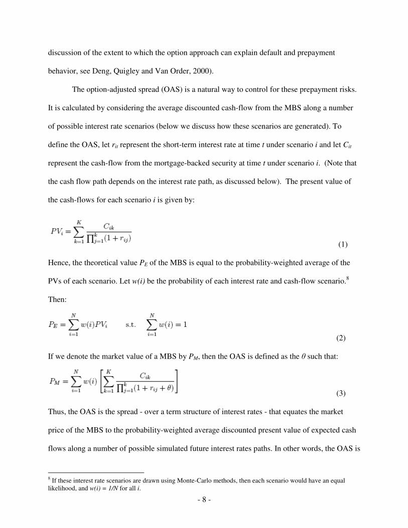
The option-adjusted spread (OAS) is a natural way to control for these prepayment risks.

It is calculated by considering the average discounted cash-flow from the MBS along a number

of possible interest rate scenarios (below we discuss how these scenarios are generated). To

define the OAS, let rit represent the short-term interest rate at time t under scenario i and let Cit

represent the cash-flow from the mortgage-backed security at time t under scenario i. (Note that

the cash flow path depends on the interest rate path, as discussed below). The present value of

the cash-flows for each scenario i is given by:

(1)

Hence, the theoretical value PE of the MBS is equal to the probability-weighted average of the

PVs of each scenario. Let w(i) be the probability of each interest rate and cash-flow scenario.8

Then:

(2)

If we denote the market value of a MBS by PM, then the OAS is defined as the θ such that:

(3)

Thus, the OAS is the spread - over a term structure of interest rates - that equates the market

price of the MBS to the probability-weighted average discounted present value of expected cash

flows along a number of possible simulated future interest rates paths. In other words, the OAS is

8 If these interest rate scenarios are drawn using Monte-Carlo methods, then each scenario would have an equal likelihood, and w(i) = 1/N for all i.

- 9 -

the number of basis points θ that the discount curve needs to be adjusted upwards until the

theoretical price calculated using the “adjusted term structure” matches the market price of the

security.

It is common to use an interest-rate model based on the LIBOR swap curve9 for the

projection of rit in which case the OAS is referred to as the swap-OAS. LIBOR is the most

appropriate discount rate for most financial market participants who balance mortgage

investments with other non-government investments. LIBOR thus provides a measure of the

opportunity cost of most investors. Fabozzi and Mann (2001) argue that “funded investors use

LIBOR as their benchmark interest rate. Most funded investors borrow at a spread over LIBOR.

Consequently, if the LIBOR swap curve is used as the benchmark interest rate, the OAS reflects

a spread relative to their funding costs.”10

To make the OAS operational, multiple paths of future interest rates must be generated

using a model of interest rates. The cash-flows from the underlying mortgages can then by

calculated using the generated interest rates. Three swap-OAS series are used in this paper. We

first focus on a Bloomberg series which is widely used by market participants. The interest rate

path and cash flow path for this series are calculated using the Bloomberg “two-factor interest

rate” and “prepayment” models. We show that the results are robust to using two other swap-

OAS series which are based on different models (one by Barclays Capital, the other by Deutsche

Bank). The results from using these series are very similar to those obtained using the

Bloomberg series. The OAS can also be calculated using an interest-rate model based on

9 By the LIBOR swap curve we mean the swap rate as a function of the maturity of the interest rate swap. The swap rate is the rate paid by a fixed-rate payer in return for receiving floating rate three-month LIBOR rolled over during the maturity period of the swap. To emphasize that LIBOR is the floating rate side of the interest rates swaps in this paper we sometimes use the term LIBOR-swap. 10 Belikoff et al. (2010) also address this issue. They argue that using the LIBOR swap curve has the additional advantage that “the swap market is quoted more uniformly and more densely [than the treasury market]'', which helps with calibrating the interest rate model used to determine the OAS. Consequently “the mortgage market has evolved to value securities relative to the swap market.”

- 10 -

Treasury securities rather than LIBOR, and we also consider this alternative measure, which we

call Treasury-OAS in our analysis. However, Treasury rates and interest rate swap rates behaved

quite differently during the financial crisis and some of the results are different for this

alternative as we discuss below.

The interest rate model used to compute the Bloomberg OAS series, which is described

in Belikoff et al. (2010), is a time series model which assumes no-arbitrage conditions on the

term structure of interest rates. For the swap-OAS the no-arbitrage conditions are imposed using

the LIBOR swap curve, and for the Treasury-OAS the no-arbitrage conditions are imposed using

the Treasury Constant Maturity curve. Brigo and Mercurio (2006) discuss the value of using

more than one factor in such time series models for the interest rates as well as the rationale for

imposing no-arbitrage conditions. Rudebusch (2010) discusses the benefit of adding macro-

variables to these interest rate models.

The prepayment model, also described in Belikoff et al. (2010), takes account of

refinancing as well as housing turnover, curtailment (when the debtor elects to pay more than the

required mortgage payment) and default. Refinancing is the major interest-rate dependent

component. Prepayment increases when interest rates are low relative to the MBS's coupon, but

is also affected by credit quality (borrowers with poor credit are less able to refinance), a “media

effect” (prepayment jumps when rates hit historic lows), and a “burnout effect” (pools that have

experienced substantial prepayment are less likely to prepay in the future, since those members

who are most likely to prepay have been removed). Housing turnover is modeled with a

seasonally-adjusted turnover rate modified by a lock-in effect in which housing turnover is

reduced when it is more expensive to close out an existing mortgage. Further adjustments are

- 11 -

made to take account of the fact that prepayments first tend to increase and then level off over

time.11

Figure 3 shows the Bloomberg swap-OAS, the Treasury-OAS and the primary mortgage

spread over Treasuries.12 The gap between the OAS series and the primary mortgage spread

partially capture changes in prepayment risk. The gap between the swap-OAS and the Treasury-

OAS is driven by movements of the Treasury term structure relative to the swap curve term

structure as we discuss further below.

2.2 Controlling for Default Risk

While the prepayment models underlying the OAS endeavor to control for prepayment

risk, they do not control for default risk. Controlling for the default risk of agency-insured MBS

is necessary to ensure that the decline in spreads in the OAS in 2009 was not driven by a decline

in the default risk of the underlying securities. Finding a good, uncontaminated measure for

default risk, however, is not easy. In the case of agency-insured MBS, the default risk is not only

related to the default risk of the underlying mortgages, but also to the potential of the insuring

agency being unable to meet its guarantee obligations. The ability to fulfill such an insurance

pledge is a function of the health of the housing market and of a number of political factors that

determine whether the government would eventually act as a backstop to the guarantees. This

uncertainty is more relevant for the GSEs Fannie Mae and Freddie Mac than for Ginnie Mae,

which has the full faith and credit backing of the United States government.

11 More details on the computation of option-adjusted spreads can be found in Kupiec and Kah (1999) and in Windas (1996). 12 In particular, the swap-OAS is the NOASFNCL.IND series and the Treasury-OAS is the MOASFNCL.IND series in Bloomberg. Both series capture the OAS of FNMA 30 Year Current Coupon MBS, and are used widely by market participants. The swap-OAS uses the S23 swap curve and the Treasury-OAS uses the constant maturity treasury (CMT) curve.

- 12 -

A good measure of the default risk of GSE-insured MBS is the credit default swap (CDS)

series on the debt issued by the insuring institutions. When there is an increased risk of default of

GSE-debt, as measured by higher costs for CDS on that debt, the risk that the GSEs will not be

able to fulfill their insurance pledge increases. Consequently, secondary market spreads on

agency-insured MBS will increase. Unfortunately, placing Fannie Mae and Freddie Mac into

conservatorship on September 7, 2008 was a trigger-event for outstanding CDS, so the data

series stops at that time. To our knowledge, no new CDS series have emerged since then that

would allow us to directly measure GSE default risk.

An alternative proxy for the default risk of Fannie and Freddie is the spread between GSE

debt and U.S. Treasury securities. One such series is the spread between 5-year Fannie Mae

bonds and U.S. Treasury active (on-the-run) securities.13 There are some concerns that such bond

spread series might be picking up liquidity effects as well as changes in default risk

(Krishnamurty, 2010). Figure 4 shows this bond spread series together with the associated CDS

series prior to its discontinuation. For the time-period that the two series coexist, they are highly

correlated, which suggests that the bond spread series does pick up changes in the default risk of

GSE-insured MBS, and does not just capture liquidity or other effects. Another complicating

factor, however, is that in late 2008 the Fed also embarked on a program to purchase agency

debt. While these interventions capture a much smaller fraction of the market than the purchases

of agency-insured MBS, they may contaminate the usefulness of bond spreads as a pure measure

of agency default risk during this period. To deal with this problem we take two approaches.

First, we instrument for the bond spread series with three instrumental variables: the level

of the Case-Shiller house price index, the change in this index, and Moody's AAA bond index.14

13 This series is available with the Bloomberg Ticker FNMGVN5.IND. 14 Moody's Long-Term Corporate Bond Yield Averages are derived from pricing data on a regularly replenished population of corporate bonds in the U.S. market, each with current outstandings over $100 million. The bonds have

- 13 -

We interpolate the monthly Case-Shiller index data to get weekly observations. A lower level of

the house price index and a large decline in the index should indicate a higher degree of

mortgage default risk. Falling house prices will push borrowers into negative home equity,

increasing their incentives for strategic default, and thus increasing the risk of mortgage default.

The Moody's AAA bond index captures the general degree of riskiness in the credit markets.

Because these instruments are unlikely to be affected by Fed purchases of GSE debt or MBS and

are highly correlated with the bond spread (the first stage regression has an F-Statistic of 99.92),

they are good instruments in our view.15 In addition, beyond its effect through capturing

increased risk in the housing credit market, neither of the instruments should have a significant

effect on the default probability of GSE-debt. Thus the exclusion restrictions are likely to be met.

We also ran robustness checks which use the CDS spreads for Bank of America, Wells Fargo,

Citigroup and JP Morgan—four large mortgage lenders in the US—to instrument for the GSE

debt spread, in place of the Moody’s AAA index. The results are very similar to those reported

with the Moody’s AAA index as the instrument.16

In a second approach, we use the spreads of Fannie Mae's Subordinated Benchmark note

series to proxy for credit risk. Since the Fed's GSE debt purchases were focused on the senior

debt market, they are less likely to have contaminated this subordinated debt as a proxy of risk.

Fannie Mae started issuing subordinated debt in 2001, with the expressed goal of “enhancing

market discipline, transparency and capital adequacy.” The subordinated debt series is unsecured

maturities as close as possible to 30 years; they are dropped from the list if their remaining life falls below 20 years, if they are susceptible to redemption, or if their ratings change. 15 One may be concerned that since the Moody's AAA index contains corporate debt, which did not suffer as much during the crisis, that it will not pick up the adequate default risk. In addition, there might also be concerns that it could be affected through a portfolio balance channel. While we do not believe that this is very likely, a robustness check of our results, in which we drop the index from our list of instruments, shows that the inclusion of the index does not affect our conclusions materially. 16 The results are available on request. The series are CDS series on 5-year Senior Bonds. They have the the following Bloomberg Tickers: BOFA CDS USD SR 5Y Corp, WELLFARGO CDS USD SR 5Y Corp, CINC CDS USD SR 5Y Corp and JPMCC CDS USD SR 5Y Corp

- 14 -

and ranks junior in priority of payment to all senior creditors, so “the price is sensitive to how the

market views our [Fannie’s] financial situation.” (Fannie Mae, 2001). Since MBS guarantees

rank pari passu to senior bonds, the subordinated debt will only be repaid if the MBS insurances

issued are fulfilled. This means that an increase in the subordinated debt spreads should signal an

increase in the probability of default for the GSE-insured MBS. The downside of looking at the

subordinated debt series is its very small volume, which is usually around $1 billion per

issuance, and not comparable in liquidity to the senior GSE bonds. Therefore, the pricing of

these securities may conflate liquidity elements with credit risk elements. Figure 4 compares the

development of the bond spread series with the subordinated debt spread series17 - it appears as if

the subordinated debt spread series moves more dramatically, especially in the period running up

to the conservatorship of Fannie and Freddie, and may thus be more able to pick up changes in

default risk.18

3. Empirical Analysis

In reporting our results we first consider the swap-OAS and the simple spread of MBS

yields over swap rates. Second, we consider the Treasury-OAS and the simple spread of MBS

yields over Treasury yields. Third we discuss shifts in the swap-spread (the spread between swap

rates and Treasury rates of the same maturity) that can help to understand the differences in the

detected impact of the MBS program on the swap-OAS and Treasury-OAS.

17 Spread of the Fannie Mae Subordinated Benchmark Series, Maturity on 5.1.2013, Volume: $1 billion (Bloomberg Ticker: FNMA 4.625 05/01/13 Corp) over 5-year Treasury. 18 It is possible that during this time period, and the event surrounding the conservatorship, there were both changes in the probability of default as well as the expected loss given default, which might affect CDS spreads and bond spreads differentially.

- 15 -

3.1 Spreads over LIBOR-Swaps

In the basic model, the option-adjusted spread is a function of the various measures of

default risk discussed in section 2.2 (interest rate spreads on Fannie Mae senior debt as well as

Fannie Mae subordinated debt, both with and without instruments) and the stock of GSE-insured

MBS held by Fed and Treasury as a percentage of the total market (about $5 trillion). Both the

OAS and the other spreads are measured in basis points (1/100 of a percentage point). The

observations are at a weekly frequency. For higher frequency series, we take the average of the

observations for that week. The estimation period is the beginning of 2007 through June 2010.

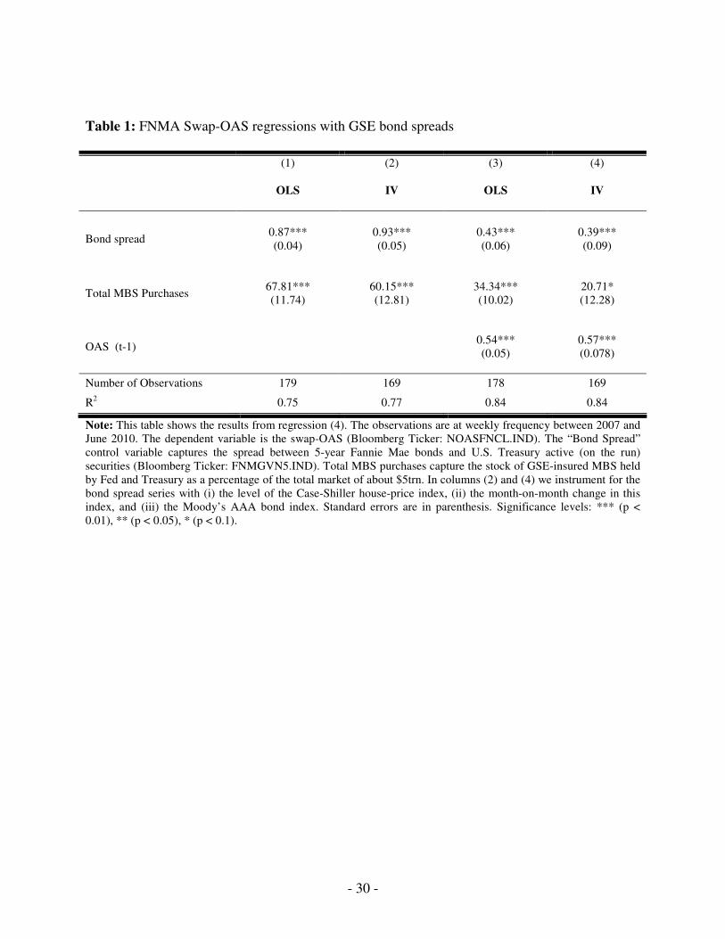
In Table 1 we report the regression results which show the impact of MBS purchases on

the swap-OAS using the GSE debt spread as the control variable. We ran regression equation (4),

with the swap-OAS as the dependent variable:

OASt = α + β1 * GSE_Spreadt + β2 * MBS_Purchasest + εt (4)

Recall that we do not need to proxy for prepayment risk, since this is already removed from the

OAS series. In columns (1) and (2) we show the OLS and instrumental variable results. In

columns (3) and (4) we also include the lagged value of the OAS series, to allow for the

possibility that the effects of the purchases are distributed over time.

Observe in Table 1 that the OAS moves closely with the bond spread, just as theory

would predict: The OAS increases when the perceived probability of default increases. However,

as measured by the coefficient on the MBS purchase volume, the impact of the purchases on the

OAS was either significantly positive or insignificantly different from zero. In this specification

there is no evidence that the increase in the MBS purchases led to a reduction in mortgage

- 16 -

interest rate spreads as measured by this conventional OAS measure, once changes in default-

risk are controlled for.

Table 2 is analogous to Table 1 except that we control for default risk using the

subordinated debt series rather than the GSE debt spread. Again, the coefficients on the total

volume of MBS purchased are either positive or statistically insignificantly different from zero.

Another possible specification includes a dummy variable for whether or not there was an

MBS purchase program along with the variable for the volume of purchases:

OASt = α + β1 * GSE_Spreadt + β2* MBS_Purchasest + β3 * I{Program Event},t + εt (5)

The results are shown in Table 3 which reports the effects of four different “Program

Event” dummy variables. In each regression the dummy is set to 0 at the start of the sample

period and then increased to 1 at a later date. In column (1) the dummy is set to 1 starting in

September 2008, when the Treasury started buying MBS and Fannie and Freddie were taken into

government conservatorship. In column (2) the dummy is set to 1 starting in January 2009 when

the Fed purchases of MBS started. In column (3) the dummy is set to 1 starting with the

announcement of the Fed's MBS purchase program on November 25, 2008. In column (4) we

also consider the impact of the announcement of the program's expansion by the Fed on March

18, 2009. On this date it was announced that the Fed would more than double the size of the

program, from $500 billion to $1.25 trillion.

The estimated coefficients in Table 3 do not indicate that either the program's existence

or the volume of purchases had a statistically significant negative effect on the swap-OAS. The

coefficients are insignificant or positive.

- 17 -

To understand why the MBS program’s volume or existence do not pick up an effect on

the swap-OAS, it is useful to consider the residuals of regressions of the OAS series on the bond

spread series (the risk indicator), without including the MBS explanatory variables. Figure 6

shows the residuals from such a regression for the swap-OAS series, along with the actual and

predicted swap-OAS series over the sample period. Notice that the residuals through this whole

period remain fairly evenly spread around zero. Movements in prepayment risk (as measured by

swap-OAS) and default risk (as measured by agency debt spreads) account for the major

movements in mortgage spreads. Little remains to be explained by the MBS purchases. This is

the reason why the coefficient on MBS purchases is very small in the swap-OAS regressions.

One possible concern with the analyses presented above is that the option-adjusted spread

relies on the quality of the Bloomberg prepayment and interest rate models used to construct the

OAS.19 Below we present two robustness checks to the previous analysis. In the first robustness

check we use two alternative swap-OAS series as dependent variables to remove prepayment

risk. These alternative series were constructed using different interest rate and prepayment

models. We use (i) an OAS series for 30 Year FNMA Current Coupon MBS computed by

Barclays Capital and (ii) an OAS series for a monthly-rebalanced index of agency-MBS,

compiled by Deutsche Bank (Bloomberg Ticker: DBIQ US TBA MBS OAS Libor).20 Figure 7

plots the two alternative OAS series and the Bloomberg OAS series. Up to the end of 2009 both

the Barclays and the Bloomberg OAS series co-moved very closely, suggesting that the models

used by Bloomberg and Barclays Capital were rather similar (both series construct OAS for 30

19 One might be concerned about this since during the crisis OAS calculations became particularly difficult to perform. Falling house prices and resulting negative home equity lowered the probability of refinancing, as did the tightening of lending standards and the market exit of a number of important mortgage lenders. This suggests that models that were not adequately updated would likely overstate the value of the prepayment option. In addition, during the crisis the dynamics of the swap curve and the Treasury curve might have changed, complicating the use of interest rate models that were calibrated to the pre-crisis economy. 20 This index includes MBS from Fannie Mae, Freddie Mac and Ginnie Mae with durations of 15 years or 30 years. It is described at: https://index.db.com/htmlPages/MBS_Index_Guide_V.pdf.

- 18 -

Year FNMA Current Coupon MBS). However, during the last few months of the MBS program,

the OAS series computed by Barclays rose significantly more, which implies that their model

valued the prepayment option less than the Bloomberg model. The Deutsche Bank series does

not capture the OAS of a single security, but of an index of MBS. Before the crisis this OAS was

higher than that of the 30 Year FNMA Current Coupon MBS. During the crisis, the co-

movement with the MBS index provided by Bloomberg increased significantly.

In Table 4 we repeat the key regressions from Table 3 using the Barclays swap-OAS

series. Notice that the coefficient on the total volume of MBS purchased by Fed and Treasury is

statistically significant and positive. This finding relative to the Bloomberg OAS-Spread

regressions is not surprising, since the Barclays OAS-series increased at a faster rate than the

Bloomberg OAS-series during the first months of 2010, while the Fed continued to purchase

more MBS during that period. The coefficients on the program announcements are negative;

however, they are very small and the net impact of the announcement effect and the volume

effect is positive. Thus, results using this alternative OAS series do not provide any evidence that

the Fed’s MBS purchase program had an impact in reducing mortgage spreads, after controlling

for prepayment risk and default risk.

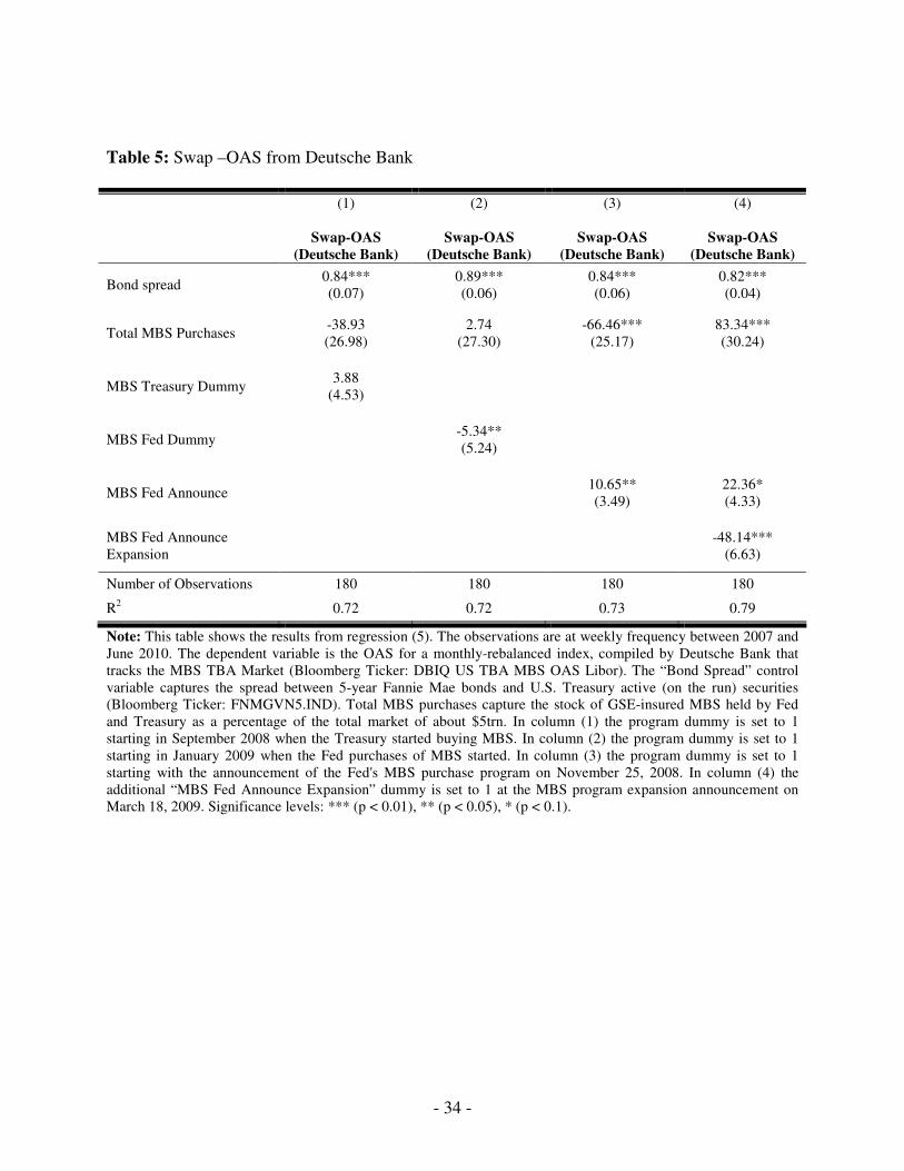
In Table 5 we present a similar set of regressions, using the OAS series provided by

Deutsche Bank as the dependent variable. As before, none of the specifications suggest a

significant reduction in option-adjusted spreads of agency-MBS as a result of either the existence

of the program, or its volume, after we have controlled for changes in prepayment risk and

default risk. The results in Column (4) show a significant negative coefficient on the

announcement dummy for the program’s expansion. However, this estimated coefficient is less

in absolute value than the estimated positive coefficient on the dummy for the announcement of

the initiation of the program.

- 19 -

A second set of robustness checks considers regressions where the secondary MBS

market spread is the left-hand side variable, without attempting to control for changes in

prepayment risk. One interpretation of this is that the value of the prepayment option is assumed

to be zero.21 In addition, if the Fed’s actions did contribute to a decline in prepayment risk, we

would like to measure this contribution to an overall decline in mortgage rates. In Table 6 the

specific dependent variable is the spread of the secondary market yield of 30 year FNMA MBS

over the 10-year swap rate. The results are consistent with the findings using the option-adjusted

spreads: The program dummies are positive, and the volume of purchases is never statistically

significant. Again, after attempting to control for default risk using the bond spreads, it does not

appear as if the program significantly lowered secondary market spreads of agency-insured

MBS.

3.2 Spreads over Treasury Rates

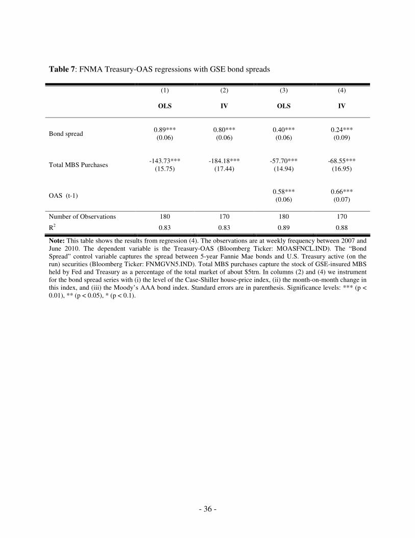
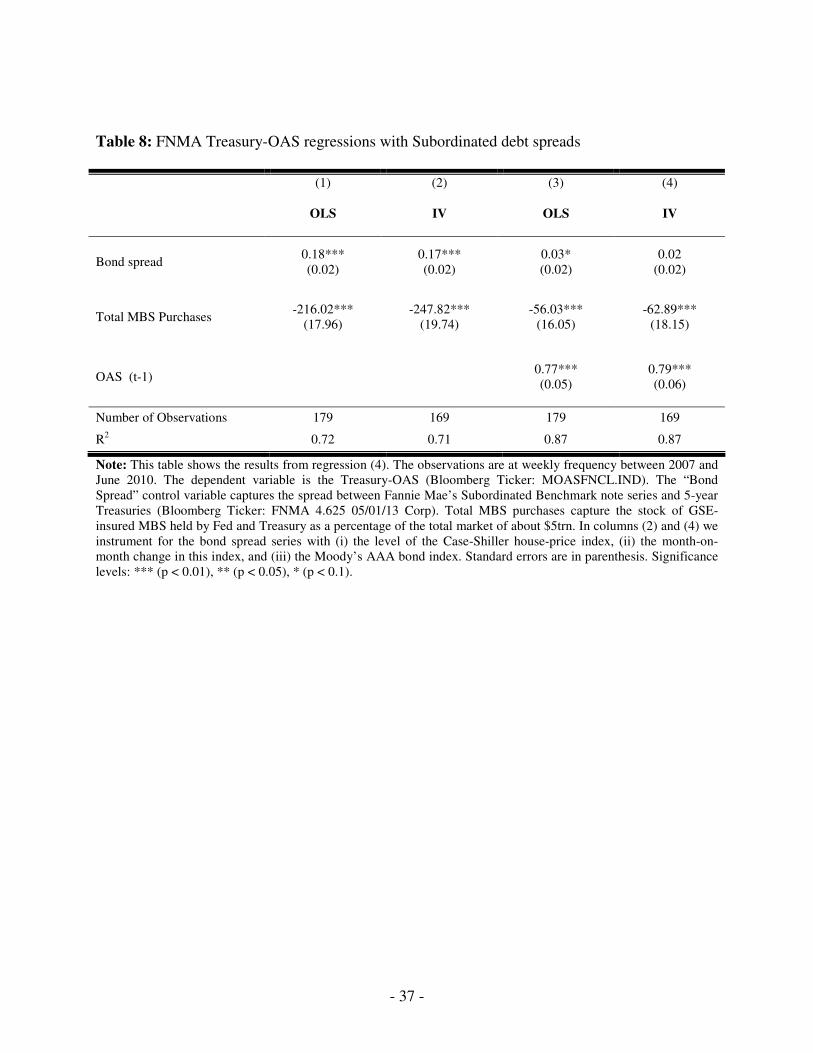
Tables 7 and 8 consider the same regressions as Tables 1 and 2 except that Treasury-

OAS, replaces swap-OAS as the dependent variable. Here the sign of the coefficient on the MBS

purchase volume shifts from positive to negative and statistically significant indicating that the

purchases have a negative effect on the Treasury-OAS. According to the estimated regression

coefficient in column (2), a purchase of $500 billion worth of MBS (approximately 10% of the

market) is associated a reduction in the Treasury-OAS of 18.4 basis points.

To better understand this estimated effect of the program, Figure 7 (which is analogous to

Figure 5 for the swap-OAS), shows the residuals from the regression of the Treasury-OAS on the

default-risk indicator. Here we see that the residuals are below zero for almost all of 2009, which

is what is being picked up by the MBS purchase coefficient. However, note that the residuals

21 Given that we argued in footnote 19 that model misspecification most likely led to an overvaluation of the prepayment option, this specification can provide a bound on the error resulting from valuing this option incorrectly.

- 20 -

show little trend movement throughout 2009, as the Fed's and the Treasury's MBS stock

continuously grew in size. If the actual volume of purchases was a partial driving factor, we

would expect residuals to become significantly more negative over time, as purchases expanded.

Rather, it appears as if there was a single downward shift in residuals without a further

effect from conducting actual purchases. This suggests that the specification that includes

program dummies might be superior. Table 9 introduces the same program-dummies as Table 3,

using the Treasury-OAS as the dependent variable. The actual volume of the MBS held by Fed

and Treasury appears to have no statistically significant effect on the Treasury-OAS. However,

unlike the swap-OAS regressions, the coefficient on the dummy variables in these regressions

indicates an effect of the existence or the announcement of the MBS purchase program. The

estimated coefficients imply a negative effect of about 30 basis points on the Treasury-OAS.

To examine the robustness of this finding we looked at the secondary market spread over

Treasuries. As shown in Table 10 a regression with the spread of the FNMA secondary market

rate over constant maturity 10-year Treasury rates also shows a statistically significant negative

effect of the announcement of the program of about 30 basis points, without a significant further

effect due to the volume of the program. This effect is very similar to the effect detected on the

Treasury-OAS.22

3.3 Did the MBS Program Make the Implicit Guarantee More Explicit?

As another robustness check we examined whether the absence of size effects and the

presence of program effects on Treasury-OAS might be due to the program's mere existence

signaling to the market that federal government guarantees of the GSEs had become more likely.

22 This suggests that any decline in the Treasury-OAS can be attributed more to changes in the default risk than to

an increase in the value of the prepayment option..

- 21 -

If investors believed that the government would always bail out Fannie and Freddie, despite the

lack of explicit “full faith and credit” insurance, mortgage spreads over Treasuries would not

have increased in 2007 and 2008 nor have remained high after the Federal government takeover.

The fact that spreads were positive suggests that market participants attached some likelihood to

the government not bailing out Fannie and Freddie (in addition to some differences in the

liquidity of the two securities). By directly purchasing GSE debt and GSE-insured MBS, the Fed

increased its own financial exposure to the GSEs, increasing the perceived strength of the

guarantee. For a discussion of the public's perception of U.S. government guarantees for GSEs,

see Passmore (2005).

To try and separate the impact that these “implicit guarantee” effects had on the OAS

from possible effects related to a provision of liquidity to mortgage markets, we analyze the

development of the option-adjusted spread on MBS that are guaranteed by Ginnie Mae. Ginnie

Mae securities are the only MBS that are explicitly guaranteed by the full faith and credit of the

United States government. If Fannie Mae OAS declined significantly more following the

announcement of the MBS purchase program than Ginnie Mae, then this is evidence for an

“implicit guarantee” explanation of any observed decline in spreads.

In Table 3 we analyzed the swap-OAS and in Table 9 the Treasury-OAS of Fannie Mae

securities. In Tables 11 and 12 we repeat the same regressions, but use the OAS on Ginnie Mae

securities as the dependent variable.23 As was the case with the swap-OAS on Fannie Mae MBS

in Table 3, when analyzing the swap-OAS of Ginnie Mae MBS, we find an incorrectly signed

effect. The coefficients suggest that the program announcement, program start and program

volume all contributed to an increase in the spread, while the effects of program volume are not

statistically significant. When looking at the effects on the Treasury-OAS of Ginnie Mae MBS,

23 We use the NOASGNSF.IND series from Bloomberg for the swap-OAS on 30-year Ginnie Mae insured MBS, and the MOASGNSF.IND series for the Treasury-OAS series.

- 22 -

we find effects that are between 1/3 and 1/2 of the size of the effect on the Fannie Mae Treasury-

OAS.24 The results thus suggest that at least 50% of the observed fall in Treasury-OAS on

mortgage-backed securities guaranteed by Fannie Mae could be attributed to the “implicit

guarantee” effect. This leaves at most a decline of about 15 bps to be explained by the MBS

purchase program.

If this “implicit guarantee” effect is indeed a key channel through which the MBS

purchases and GSE debt purchases affected mortgage spreads,25 a significantly more

straightforward way to achieve the same goal would have been to extend, formally and

explicitly, the full faith and credit of the United States to Fannie and Freddie, in a similar fashion

as it is already extended to Ginnie Mae. Moreover, if the implicit guarantee was the channel,

then similar MBS purchase programs used in the future are are not likely to have any impact on

spreads.

4 A Shift in the Swap Spread

The results in the previous section reveal a strong positive effect of risk factors and no

negative effect of the volume of MBS purchases on mortgage spreads. These results are robust to

alternative measures and specifications. The results also reveal a marked difference in the

estimated effect of the MBS program’s existence or announcement on spreads over swaps rates

versus spreads over Treasury rates: Program dummies show no negative effect of the program on

the swap-OAS and about a 30-basis point negative effect on the Treasury-OAS. This result is

also robust to alternative measures and specifications.

24 These results survive in a specification where we drop the total volume of MBS purchased from the regression. 25 An “implicit guarantee” channel might also have contributed to the decline in the bond spreads, which we use to control for the default risk of the MBS.

- 23 -

This difference in the estimated dummy coefficients in the regression equation for

spreads over swaps versus spreads over Treasury rates implies certain relative movements of

swaps and Treasury rates during this period. In particular it implies that the spread between

swaps rates and Treasury rates—commonly referred to as the swap spread— should have

narrowed during this period. To show this simply, we can abstract from maturity differences or

the term structure, and let M = mortgage rate, S = swap rate, and T = Treasury rate. Then the

two mortgage spreads discussed in the previous section are M-S and M-T, and the swap spread is

S-T. Our empirical results show that the M-S spread was unchanged during the period of the

program (after controlling for prepayment and default risk) while the M-T spread decreased. So

the implication is that (M-T) - (M-S) decreased, which means of course that the swap spread S-T

decreased.26

In fact the swap spreads did decrease during this period. We examined the 1-year, 2-year,

5-year and 10-year swap spreads. Figure 9 shows the 10-year swap spread, or the difference

between the 10-year swap rate and the 10-year constant maturity Treasury rate. Clearly there

was a significant down shift in swap spread during this time period. The spread averaged about

0.5 percent from 2005 through 2007 and about 0.1 percent from the start of 2009 through June

2011. The story is similar for the swap spreads at other maturities, though the shorter maturities

increased by a larger amount during the panic in late September and early October 2008 before

decreasing.27

26 To consider the whole term structure you can use the derivation of the OAS in equation (3). The interest rate (rit) used for computing the OAS (θ) is based on the LIBOR swap curve in the case of the swap-OAS while it is based on the Treasury yield curve in the case of the Treasury-OAS. The difference between these two curves is due differences in the swap spreads at various maturities. 27 During the panic the TED spread (3-month LIBOR over 3-month Treasury bill rates) and the LIBOR-Overnight Index Spread (OIS) were also spiking. See Smith (2010) and Taylor and Williams (2009) for a discussion of movements in LIBOR-OIS around the period of the panic.

- 24 -

The decline in the swap spread shown in Figure 9 is well-known to traders and investors

in the swap and Treasury markets. The most commonly cited explanation28 for the decline is the

huge increase in Treasury borrowing relative to private sector borrowing as the federal deficit

increased sharply when the economy went into a sharp downturn in late 2008. This increased

the demand for Treasury borrowing and decreased the demand for private sector borrowing;

hence, according to this explanation the spread between swap rates and Treasury rates narrowed.

In support of this explanation, the Treasury Borrowing Advisory Committee (2010) reported that

until October 2008, the Treasury had been adding incrementally to coupon auction sizes. In

October 2008, Treasury surprised the market with a $40 billion of 2015/18 issues, which was

followed by a rapid rise in coupon issuance for a full year.

Given the algebraic link between the three spreads (M-S, M-T, and S-T), at least two

possible explanations for the decline in the swap spread (S-T) thus emerge from our analysis.

The first possible explanation—discussed in the previous section of this paper—is that the MBS

program reduced mortgage spreads over Treasuries but did not reduce mortgage spreads over

swaps and thereby led to a decline in the swap spread. The second explanation—discussed in the

Treasury Borrowing Advisory Committee Report (2010) and elsewhere—is that a large increase

in the supply of Treasury debt drove down the swap spread and thereby created a differential

between mortgage spreads over swap rates and mortgage spreads over Treasury rates.

There are potentially important timing differences which might help to distinguish

between the two explanations. For example, the second explanation implies that the shift in the

swap spreads would occur in October 2008 when Treasury issuance rose, while the first

explanation implies that the swap shift would begin at the time of the MBS program

announcement or start-up. In Figure 9 we have drawn a vertical line at the week ending

28 See, for example, the Quarterly Treasury Borrowing Advisory Committee Report of May 2010.

- 25 -

November 15, which was before the November 25th announcement of the Fed’s purchase

program. In Figure 10 we show daily observations on that same swap spread. Most of the

movement in the spread occurred before the announcement of the program by the Fed. While

this provides some evidence in favor of the second hypothesis, rigorous testing between these

two explanations will require additional research including further specifying and exploring the

second explanation, which is beyond the scope of this paper.

5. Conclusion

In this paper we endeavored to estimate the quantitative impact of the Federal Reserve's

mortgage-backed securities purchase program on mortgage interest spreads using a multivariate

statistical framework which takes account of other possible influences on spreads. We controlled

for two other possible influences on mortgage spreads: changes in prepayment risk and changes

in default risk. Our results can be summarized as follows:

• Using conventional option-adjusted spreads (OAS) from Bloomberg based on LIBOR

swaps to control for prepayment risks, it is difficult to detect a significant effect of the

MBS purchases. Movements in prepayment risk and particularly movements in default

risk explain virtually all of the movements in mortgage spreads, as captured by the OAS

relative to the swap curve. We find similar results when using other swap-OAS series

compiled by Barclays and Deutsche Bank, as well as when considering the secondary

market MBS spread without controlling for possible changes in prepayment risk.

• A statistically significant effect on mortgage spreads - about 30 basis points - can be

found if one uses an alternative measure of OAS based on the Treasury yield curve, but

even with this measure the volume of purchases has no effect over and above the mere

announcement or existence of the program. In other words the impact has not increased

- 26 -

with the additional purchases of MBS since the start of the program. We find a similar

effect when we consider the secondary market MBS spread of MBS over Treasuries,

without attempting to control for prepayment risk.

• When also analyzing the impact on the OAS of MBS guaranteed by Ginnie Mae, which

has the U.S. government's explicit full faith and credit guarantee, we find evidence for the

suggestion that about 50% of the 30 basis points decline in Treasury-OAS for MBS

guaranteed by Fannie Mae can be attributed to what we call the “implicit guarantee”

effect. This suggests that about 15 basis points of the decline in Treasury-OAS can be

explained by increased liquidity in agency-insured MBS markets.

• Finally we showed that the estimated negative impact on the Treasury-OAS compared

with the estimated zero impact on the swap-OAS implies a downward shift in the swap

spread or the difference between swap rates and Treasury rates during this period. Such a

shift did indeed occur and has been noted by market participants, who have offered an

explanation unrelated to the MBS purchase program. While timing differences provide

support for this alternative explanation, further research is required to discriminate

rigorously between these hypotheses. We hope that the information in this study will be

of value in such research.

Analyzing the effectiveness of the MBS purchase program is very difficult. The creation of

adequate counterfactuals is complicated by the simultaneous government interventions in a large

number of markets. Furthermore, the conservatorship-status of the GSEs has contaminated many

of the relevant GSE-default risk proxies that are most important to control for when analyzing

the development of spreads on GSE-insured MBS. Our analysis has used a variety of different

approaches to proxy for this risk, each with its own problems. Nevertheless, on balance this

paper suggests that the impact of the Fed's MBS purchase program on mortgage spreads has been

- 27 -

small and uncertain, once the effects of default risk and prepayment risk have been taken into

account.

While this paper is unlikely to be the final word on the program's effectiveness, our

empirical results thus raise questions about the ability of central banks to conduct price-keeping

operations reliably by increasing and decreasing asset purchases in particular markets. They also

raise doubts about the benefits in terms of lower mortgage interest rates of further increases in

the size of the Fed's MBS portfolio or about the costs in terms of higher interest rates of

gradually reducing the size of that portfolio.

- 28 -

References

• Aït-Sahalia, Yacine, Jochen Andritzky, Andreas Jobst, Sylwia Nowak and Natalia Tamirisa. (2010). “Market Response to Policy Initiatives during the Global Financial Crisis,” NBER Working Paper 15809 (March).

• Belikoff, Alexander, Kirill Levin, Harvey Stein and Xusheng Tian. (2010). “Analysis of Mortgage Backed Securities: Before and After the Crisis.” Bloomberg LP, Version 2.2.

• Bernanke, Ben. (2009). “The Crisis and the Policy Response.” Stamp Lecture, London School of Economics, London, England, January 13, 2009.

• Boudoukh, Jacob, Mathew Richardson, Richard Stanton and Robert Whitelaw. (1999). “The Pricing and Hedging of Mortgage-Backed Securities: A Multivariate Density Estimation Approach.” In Advanced Fixed Income Valuation Tools, edited by N. Jegadeesh and Bruce Tuckman, Chapter 9. John Wiley Publishing.

• Brigo, Damiano and Fabio Mercurio. (2006). Interest Rate Models: Theory and Practice. Berlin Heidelberg: Springer Finance, 2nd Edition.

• Ciorciari, John and Taylor, John (eds). (2009). The Road Ahead for the Fed. by George Shultz, Allan Meltzer, Peter Fisher, Donald Kohn, James Hamilton, John Taylor, Myron Scholes, Darrell Duffie, Andrew Crockett, Michael Halloran, Richard Herring, and John Ciorciari. Stanford, CA: Hoover Press.

• Deng, Yongheng, John M. Quigley and Robert van Order (2000). “Mortgage Terminations, Heterogeneity and the Exercise of Mortgage Options,” Econometrica, vol. 68 (2), 275 – 307

• Duygan-Bumpt, Burcu, Patrick Parkinson, Eric Rosengren, Gustavo Suarez and Paul Willen. (2010). “How Effective Were the Federal Reserve Emergency Liquidity Facilities? Evidence from the Asset-Backed Commercial Paper Money Market Mutual Fund Liquidity Facility.” Working Paper QAU10-3, Federal Reserve Bank of Boston. April 29, 2010.

• Fabozzi, Frank and Steven Mann. (2001), “Introduction to Fixed Income Analytics.” Frank J. Fabozzi Associates.

• Fannie Mae. (2001), “2001 Annual Report”, Statement by CFO Timothy Howard

• Fuster, Andreas and Paul Willen. (2010), “$1.25 Trillion is still real money: some facts about the effects of the Federal Reserve’s mortgage market investments.” Federal Reserve Bank of Boston Discussion Paper No. 10-4.

• Gagnon, Joseph, Matthew Raskin, Julie Remanche, and Brian Sack. (2011). “The

Financial Market Effects of the Federal Reserve’s Large-Scale Asset Purchases”

International Journal of Central Banking, vol. 7(1), 3 – 44.

- 29 -

• Hancok, Diana and Wayne Passmore. (2011). “Did the Federal Reserve’s MBS Purchase Program lower mortgage rates?” Finance and Economics Discussion Series 2011 - 01, Federal Reserve Board

• Hull, John and Alan White. (1994). “Numerical procedures for implementing term structure models II.” Journal of Derivatives, vol. 2(2), 37 – 48.

• Krishnamurty, Arvind. (2010). “How Debt Markets Have Malfunctioned in the Crisis.” Journal of Economic Perspectives, vol. 24(1), 3 – 28

• Kupiec, Paul and Adama Kah. (1999). “On the Origin and Interpretation of OAS.” The

Journal of Fixed Income, vol. 9(3), 82 – 92.

• Lehnert, Andreas, Wayne Passmore and Shane Sherlund. (2006). “GSEs, Mortgage Rates, and Secondary Market Activities.” Federal Reserve Board of Governors, September, FEDS Working Paper 2006-30.

• Passmore, Wayne. (2005). “The GSE Implicit Subsidy and the Value of Government Ambiguity.” FEDS Working Paper No. 2005-05

• Rudebusch, Glenn. (2010). “Macro-Finance Models of Interest Rates and the Economy,” Federal Reserve Bank of San Francisco Working Paper, 2010-01

• Sack, Brian. (2009). “The Fed's Expanded Balance Sheet.” Remarks at the Money Marketeers of NYU, December 2, 2009. Available at:http://www.newyorkfed.org/ newsevents/speeches/2009/sac091202.html.

• Smith, Josephine. (2010). “The Term structure of Money Market Spreads during the Financial Crisis.” Working Paper, Stanford University

• Spahr, Ronald and Mark Sunderman. (1994). “The Effect of Prepayment Modeling in Pricing Mortgage-Backed Securities.” Journal of Housing Research vol. 3(2), 381 – 400.

• Taylor, John. (2009). “Empirically Evaluating Economic Policy in Real Time.” Martin Feldstein Lecture, National Bureau of Economic Research, July 10. NBER Reporter, No. 3, 2009.

• Taylor, John and John Williams. (2009). “A Black Swan in the Money Market.” American Economic Journal: Macroeconomics, vol. 1(1), 58-83.

• Treasury Borrowing Advisory Committee (2010), Presentation to the Quarterly Meeting, May 4, 2010. Available at: http://www.treasury.gov/resource-center/data-chart-center/quarterly-refunding/Documents/dc-2010-q2.pdf

• Windas, Tom. (1996). An introduction to option-adjusted spread analysis. Revised Edition. Princeton, NJ: Bloomberg Press

- 30 -

Table 1: FNMA Swap-OAS regressions with GSE bond spreads

(1) (2) (3) (4)

OLS IV OLS IV

Bond spread 0.87*** (0.04)

0.93*** (0.05)

0.43*** (0.06)

0.39*** (0.09)

Total MBS Purchases 67.81*** (11.74)

60.15*** (12.81)

34.34*** (10.02)

20.71* (12.28)

OAS (t-1)

0.54*** (0.05)

0.57*** (0.078)

Number of Observations 179 169 178 169

R2 0.75 0.77 0.84 0.84

Note: This table shows the results from regression (4). The observations are at weekly frequency between 2007 and June 2010. The dependent variable is the swap-OAS (Bloomberg Ticker: NOASFNCL.IND). The “Bond Spread” control variable captures the spread between 5-year Fannie Mae bonds and U.S. Treasury active (on the run) securities (Bloomberg Ticker: FNMGVN5.IND). Total MBS purchases capture the stock of GSE-insured MBS held by Fed and Treasury as a percentage of the total market of about $5trn. In columns (2) and (4) we instrument for the bond spread series with (i) the level of the Case-Shiller house-price index, (ii) the month-on-month change in this index, and (iii) the Moody’s AAA bond index. Standard errors are in parenthesis. Significance levels: *** (p < 0.01), ** (p < 0.05), * (p < 0.1).

- 31 -

Table 2: FNMA Swap-OAS regressions with subordinated debt spreads

(1) (2) (3) (4)

OLS IV OLS IV

Bond spread 0.24*** (0.01)

0.25*** (0.01)

0.08*** (0.02)

0.09*** (0.03)

Total MBS Purchases 22.81** (10.85)

7.81 (11.46)

3.84 (8.56)

-1.32 (9.49)

OAS (t-1)

0.67*** (0.06)

0.63*** (0.09)


R2 0.72 0.75 0.84 0.84

Note: This table shows the results from regression (4) with the subordinated debt spread replacing the GSE bond spread. The observations are at weekly frequency between 2007 and June 2010. The dependent variable is the swap-OAS (Bloomberg Ticker: NOASFNCL.IND). The “Bond Spread” control variable captures the spread between Fannie Mae’s Subordinated Benchmark note series and 5-year Treasuries (Bloomberg Ticker: FNMA 4.625 05/01/13 Corp). Total MBS purchases capture the stock of GSE-insured MBS held by Fed and Treasury as a percentage of the total market of about $5trn. In columns (2) and (4) we instrument for the bond spread series with (i) the level of the Case-Shiller house-price index, (ii) the month-on-month change in this index, and (iii) the Moody’s AAA bond index. Standard errors are in parenthesis. Significance levels: *** (p < 0.01), ** (p < 0.05), * (p < 0.1).

- 32 -

Table 3: FNMA Swap –OAS with Program Dummies

(1) (2) (3) (4)

Swap-OAS

(Bloomberg)

Swap-OAS

(Bloomberg)

Swap-OAS

(Bloomberg)

Swap-OAS

(Bloomberg)

Bond spread 0.88*** (0.05)

0.85*** (0.04)

0.84*** (0.04)

0.84*** (0.04)

Total MBS Purchases 69.73*** (20.46)

24.58 (20.21)

31.22 (19.13)

64.47** (25.67)

MBS Treasury Dummy -0.39 (3.45)

MBS Fed Dummy 10.11***

(3.88)

MBS Fed Announce 8.41* (3.50)

11.14*** (3.78)

MBS Fed Announce Expansion -10.57* (5.66)


R2 0.75 0.76 0.75 0.76

Note: This table shows the results from regression (5). The observations are at weekly frequency between 2007 and June 2010. The dependent variable is the swap-OAS (Bloomberg Ticker: NOASFNCL.IND). The “Bond Spread” control variable captures the spread between 5-year Fannie Mae bonds and U.S. Treasury active (on the run) securities (Bloomberg Ticker: FNMGVN5.IND). Total MBS purchases capture the stock of GSE-insured MBS held by Fed and Treasury as a percentage of the total market of about $5trn. In column (1) the program dummy is set to 1 starting in September 2008 when the Treasury started buying MBS. In column (2) the program dummy is set to 1 starting in January 2009 when the Fed purchases of MBS started. In column (3) the program dummy is set to 1 starting with the announcement of the Fed's MBS purchase program on November 25, 2008. In column (4) the additional “MBS Fed Announce Expansion” dummy is set to 1 at the MBS program expansion announcement on March 18, 2009. Significance levels: *** (p < 0.01), ** (p < 0.05), * (p < 0.1).

- 33 -

Table 4: FNMA Swap –OAS from Barclays Capital

(1) (2) (3) (4)

Swap-OAS

(Barclays)

Swap-OAS

(Barclays)

Swap-OAS

(Barclays)

Swap-OAS

(Barclays)

Bond spread 0.97*** (0.05)

0.92*** (0.04)

0.90*** (0.04)

0.89*** (0.04)

Total MBS Purchases 153.41***

(20.03) 150.74***

(20.33) 115.35***

(19.21) 195.62***

(24.80)

MBS Treasury Dummy -7.80** (3.36)

MBS Fed Dummy -8.23** (3.90)

MBS Fed Announce 0.05* (3.49)

6.32* (3.54)

MBS Fed Announce Expansion -25.79***

(5.43)


R2 0.74 0.74 0.73 0.76

Note: This table shows the results from regression (5). The observations are at weekly frequency between 2007 and June 2010. The dependent variable is the OAS of FNMA 30 year current coupon MBS as computed by Barclays Capital. The “Bond Spread” control variable captures the spread between 5-year Fannie Mae bonds and U.S. Treasury active (on the run) securities (Bloomberg Ticker: FNMGVN5.IND). Total MBS purchases capture the stock of GSE-insured MBS held by Fed and Treasury as a percentage of the total market of about $5trn. In column (1) the program dummy is set to 1 starting in September 2008 when the Treasury started buying MBS. In column (2) the program dummy is set to 1 starting in January 2009 when the Fed purchases of MBS started. In column (3) the program dummy is set to 1 starting with the announcement of the Fed's MBS purchase program on November 25, 2008. In column (4) the additional “MBS Fed Announce Expansion” dummy is set to 1 at the MBS program expansion announcement on March 18, 2009. Significance levels: *** (p < 0.01), ** (p < 0.05), * (p < 0.1).

- 34 -

Table 5: Swap –OAS from Deutsche Bank

(1) (2) (3) (4)

Swap-OAS

(Deutsche Bank)

Swap-OAS

(Deutsche Bank)

Swap-OAS

(Deutsche Bank)

Swap-OAS

(Deutsche Bank)

Bond spread 0.84*** (0.07)

0.89*** (0.06)

0.84*** (0.06)

0.82*** (0.04)

Total MBS Purchases -38.93 (26.98)

2.74 (27.30)

-66.46*** (25.17)

83.34*** (30.24)

MBS Treasury Dummy 3.88

(4.53)

MBS Fed Dummy -5.34** (5.24)

MBS Fed Announce 10.65** (3.49)

22.36* (4.33)

MBS Fed Announce Expansion

-48.14***

(6.63)


R2 0.72 0.72 0.73 0.79

Note: This table shows the results from regression (5). The observations are at weekly frequency between 2007 and June 2010. The dependent variable is the OAS for a monthly-rebalanced index, compiled by Deutsche Bank that tracks the MBS TBA Market (Bloomberg Ticker: DBIQ US TBA MBS OAS Libor). The “Bond Spread” control variable captures the spread between 5-year Fannie Mae bonds and U.S. Treasury active (on the run) securities (Bloomberg Ticker: FNMGVN5.IND). Total MBS purchases capture the stock of GSE-insured MBS held by Fed and Treasury as a percentage of the total market of about $5trn. In column (1) the program dummy is set to 1 starting in September 2008 when the Treasury started buying MBS. In column (2) the program dummy is set to 1 starting in January 2009 when the Fed purchases of MBS started. In column (3) the program dummy is set to 1 starting with the announcement of the Fed's MBS purchase program on November 25, 2008. In column (4) the additional “MBS Fed Announce Expansion” dummy is set to 1 at the MBS program expansion announcement on March 18, 2009. Significance levels: *** (p < 0.01), ** (p < 0.05), * (p < 0.1).

- 35 -

Table 6: Secondary Market Spread over Swap Rates

(1) (2) (3) (4)

Secondary

Market Spread

Secondary

Market Spread

Secondary

Market Spread

Secondary

Market Spread

Bond spread 0.67*** (0.08)

0.74*** (0.07)

0.71*** (0.07)

0.71*** (0.07)

Total MBS Purchases -20.96 (32.11)

-49.65 (31.96)

-37.93 (29.89)

21.18 (40.45)

MBS Treasury Dummy 12.89** (5.40)


(6.13)

MBS Fed Announce 18.23***

(5.43)

22.89*** (5.79)


-18.99**

(2.14)


R2 0.51 0.53 0.53 0.54

Note: This table shows the results from regression (5). The observations are at weekly frequency between 2007 and June 2010. The dependent variable is the spread of Fannie Mae MBS 30 Year Current Coupon (Bloomberg Ticker: MTGEFNCL.IND) over 10-year swap rates. The “Bond Spread” control variable captures the spread between 5-year Fannie Mae bonds and U.S. Treasury active (on the run) securities (Bloomberg Ticker: FNMGVN5.IND). Total MBS purchases capture the stock of GSE-insured MBS held by Fed and Treasury as a percentage of the total market of about $5trn. In column (1) the program dummy is set to 1 starting in September 2008 when the Treasury started buying MBS. In column (2) the program dummy is set to 1 starting in January 2009 when the Fed purchases of MBS started. In column (3) the program dummy is set to 1 starting with the announcement of the Fed's MBS purchase program on November 25, 2008. In column (4) the additional “MBS Fed Announce Expansion” dummy is set to 1 at the MBS program expansion announcement on March 18, 2009. Significance levels: *** (p < 0.01), ** (p < 0.05), * (p < 0.1).

- 36 -

Table 7: FNMA Treasury-OAS regressions with GSE bond spreads

(1) (2) (3) (4)

OLS IV OLS IV

Bond spread 0.89*** (0.06)

0.80*** (0.06)

0.40*** (0.06)

0.24*** (0.09)

Total MBS Purchases -143.73***

(15.75) -184.18***

(17.44) -57.70***

(14.94) -68.55***

(16.95)

OAS (t-1)

0.58*** (0.06)

0.66*** (0.07)


R2 0.83 0.83 0.89 0.88

Note: This table shows the results from regression (4). The observations are at weekly frequency between 2007 and June 2010. The dependent variable is the Treasury-OAS (Bloomberg Ticker: MOASFNCL.IND). The “Bond Spread” control variable captures the spread between 5-year Fannie Mae bonds and U.S. Treasury active (on the run) securities (Bloomberg Ticker: FNMGVN5.IND). Total MBS purchases capture the stock of GSE-insured MBS held by Fed and Treasury as a percentage of the total market of about $5trn. In columns (2) and (4) we instrument for the bond spread series with (i) the level of the Case-Shiller house-price index, (ii) the month-on-month change in this index, and (iii) the Moody’s AAA bond index. Standard errors are in parenthesis. Significance levels: *** (p < 0.01), ** (p < 0.05), * (p < 0.1).

- 37 -

Table 8: FNMA Treasury-OAS regressions with Subordinated debt spreads

(1) (2) (3) (4)

OLS IV OLS IV

Bond spread 0.18*** (0.02)

0.17*** (0.02)

0.03* (0.02)

0.02 (0.02)


(17.96) -247.82***

(19.74) -56.03***

(16.05) -62.89***

(18.15)

OAS (t-1)

0.77*** (0.05)

0.79*** (0.06)


R2 0.72 0.71 0.87 0.87

Note: This table shows the results from regression (4). The observations are at weekly frequency between 2007 and June 2010. The dependent variable is the Treasury-OAS (Bloomberg Ticker: MOASFNCL.IND). The “Bond Spread” control variable captures the spread between Fannie Mae’s Subordinated Benchmark note series and 5-year Treasuries (Bloomberg Ticker: FNMA 4.625 05/01/13 Corp). Total MBS purchases capture the stock of GSE-insured MBS held by Fed and Treasury as a percentage of the total market of about $5trn. In columns (2) and (4) we instrument for the bond spread series with (i) the level of the Case-Shiller house-price index, (ii) the month-on-month change in this index, and (iii) the Moody’s AAA bond index. Standard errors are in parenthesis. Significance levels: *** (p < 0.01), ** (p < 0.05), * (p < 0.1).

- 38 -

Table 9: FNMA Treasury – OAS with Program Dummies

(1) (2) (3) (4)

Treasury-OAS

(Bloomberg)

Treasury -OAS

(Bloomberg)

Treasury -OAS

(Bloomberg)

Treasury -OAS

(Bloomberg)

Bond spread 0.93*** (0.06)

0.90*** (0.05)

0.90*** (0.05)

0.98*** (0.05)


(23.13) -54.45** (23.14)

-71.85*** (21.80)

54.05* (30.34)


MBS Fed Dummy -11.62***

(4.44)

MBS Fed Announce -7.42* (3.95)

-22.49*** (4.34)

MBS Fed Announce Expansion -23.97***

(6.65)


R2 0.85 0.85 0.85 0.87

Note: This table shows the results from regression (5). The observations are at weekly frequency between 2007 and June 2010. The dependent variable is the swap-OAS (Bloomberg Ticker: NOASFNCL.IND). The “Bond Spread” control variable captures the spread between 5-year Fannie Mae bonds and U.S. Treasury active (on the run) securities (Bloomberg Ticker: FNMGVN5.IND). Total MBS purchases capture the stock of GSE-insured MBS held by Fed and Treasury as a percentage of the total market of about $5trn. In column (1) the program dummy is set to 1 starting in September 2008 when the Treasury started buying MBS. In column (2) the program dummy is set to 1 starting in January 2009 when the Fed purchases of MBS started. In column (3) the program dummy is set to 1 starting with the announcement of the Fed's MBS purchase program on November 25, 2008. In column (4) the additional “MBS Fed Announce Expansion” dummy is set to 1 at the MBS program expansion announcement on March 18, 2009. Significance levels: *** (p < 0.01), ** (p < 0.05), * (p < 0.1).

- 39 -

Table 10: Secondary Market Spread over Treasuries

(1) (2) (3) (4)

Secondary

Market Spread

Secondary

Market Spread

Secondary

Market Spread

Secondary

Market Spread

Bond spread 1.14*** (0.06)

0.92*** (0.05)

0.95*** (0.05)

0.94*** (0.05)

Total MBS Purchases 9.02

(21.99) -14.83 (23.62)

-33.06 (22.30)

31.78 (29.72)

MBS Treasury Dummy -30.78***

(3.69)


(4.53)

MBS Fed Announce -24.66***

(4.05) -19.59***

(4.25)


-20.83***

(6.51)


R2 0.88 0.87 0.86 0.87

Note: This table shows the results from regression (5). The observations are at weekly frequency between 2007 and June 2010. The dependent variable is the spread of Fannie Mae MBS 30 Year Current Coupon (Bloomberg Ticker: MTGEFNCL.IND) over 10 Year Treasury yields. The “Bond Spread” control variable captures the spread between 5-year Fannie Mae bonds and U.S. Treasury active (on the run) securities (Bloomberg Ticker: FNMGVN5.IND). Total MBS purchases capture the stock of GSE-insured MBS held by Fed and Treasury as a percentage of the total market of about $5trn. In column (1) the program dummy is set to 1 starting in September 2008 when the Treasury started buying MBS. In column (2) the program dummy is set to 1 starting in January 2009 when the Fed purchases of MBS started. In column (3) the program dummy is set to 1 starting with the announcement of the Fed's MBS purchase program on November 25, 2008. In column (4) the additional “MBS Fed Announce Expansion” dummy is set to 1 at the MBS program expansion announcement on March 18, 2009. Significance levels: *** (p < 0.01), ** (p < 0.05), * (p < 0.1).

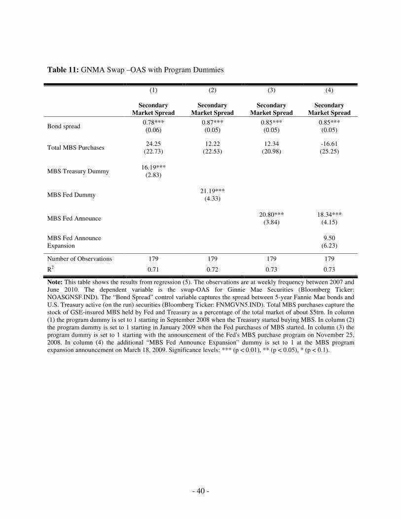
- 40 -

Table 11: GNMA Swap –OAS with Program Dummies

(1) (2) (3) (4)

Secondary

Market Spread

Secondary

Market Spread

Secondary

Market Spread

Secondary

Market Spread

Bond spread 0.78*** (0.06)

0.87*** (0.05)

0.85*** (0.05)

0.85*** (0.05)

Total MBS Purchases 24.25

(22.73) 12.22

(22.53) 12.34

(20.98) -16.61 (25.25)

MBS Treasury Dummy 16.19***

(2.83)


(4.33)

MBS Fed Announce 20.80***

(3.84) 18.34***

(4.15)


9.50

(6.23)


R2 0.71 0.72 0.73 0.73

Note: This table shows the results from regression (5). The observations are at weekly frequency between 2007 and June 2010. The dependent variable is the swap-OAS for Ginnie Mae Securities (Bloomberg Ticker: NOASGNSF.IND). The “Bond Spread” control variable captures the spread between 5-year Fannie Mae bonds and U.S. Treasury active (on the run) securities (Bloomberg Ticker: FNMGVN5.IND). Total MBS purchases capture the stock of GSE-insured MBS held by Fed and Treasury as a percentage of the total market of about $5trn. In column (1) the program dummy is set to 1 starting in September 2008 when the Treasury started buying MBS. In column (2) the program dummy is set to 1 starting in January 2009 when the Fed purchases of MBS started. In column (3) the program dummy is set to 1 starting with the announcement of the Fed's MBS purchase program on November 25, 2008. In column (4) the additional “MBS Fed Announce Expansion” dummy is set to 1 at the MBS program expansion announcement on March 18, 2009. Significance levels: *** (p < 0.01), ** (p < 0.05), * (p < 0.1).

- 41 -

Table 12: GNMA Treasury – OAS with Program Dummies

(1) (2) (3) (4)

Secondary

Market Spread

Secondary

Market Spread

Secondary

Market Spread

Secondary

Market Spread

Bond spread 0.93*** (0.06)

0.90*** (0.05)

0.90*** (0.05)

0.90*** (0.05)


(23.13) -54.45** (23.14)

-71.85*** (21.80)

-66.20** (29.88)



(4.44)

MBS Fed Announce -7.42* (3.95)

-6.98 (4.28)


-1.81 (6.55)


R2 0.85 0.85 0.85 0.85

Note: This table shows the results from regression (5). The observations are at weekly frequency between 2007 and June 2010. The dependent variable is the Treasury-OAS for Ginnie Mae Securities (Bloomberg Ticker: MOASGNSF.IND). The “Bond Spread” control variable captures the spread between 5-year Fannie Mae bonds and U.S. Treasury active (on the run) securities (Bloomberg Ticker: FNMGVN5.IND). Total MBS purchases capture the stock of GSE-insured MBS held by Fed and Treasury as a percentage of the total market of about $5trn. In column (1) the program dummy is set to 1 starting in September 2008 when the Treasury started buying MBS. In column (2) the program dummy is set to 1 starting in January 2009 when the Fed purchases of MBS started. In column (3) the program dummy is set to 1 starting with the announcement of the Fed's MBS purchase program on November 25, 2008. In column (4) the additional “MBS Fed Announce Expansion” dummy is set to 1 at the MBS program expansion announcement on March 18, 2009. Significance levels: *** (p < 0.01), ** (p < 0.05), * (p < 0.1).

- 42 -

Figure 1: Mortgage Spreads and Stock of MBS Purchases

0

50

100

150

200

250

300

350

400

0

200

400

600

800

1,000

1,200

1,400

1,600

2004 2005 2006 2007 2008 2009 2010

Primary Mortgage Market Spread (Top Line)Secondary Mortgage Market Spread (Bottom Line)Total Stock of MBS (Fed and Treasury)

Basis points Billion USD

Note: This figure shows the primary market mortgage spread and the secondary market mortgage spread, constructed as described in footnote 2. It also shows the total stock of MBS purchases by the Fed and Treasury, constructed as described in footnote 3.

- 43 -

Figure 2: Monthly Flows of GSE-insured MBS Issues and Shares bought by Fed and Treasury

-25,000

25,000

75,000

125,000

175,000

Jul-

08

Aug-

08

Sep-

08

Oct-

08

Nov-

08

Dec-

08

Jan-

09

Feb-

09

Mar-

09

Apr-

09

May-

09

Jun-

09

Jul-

09

Aug-

09

Sep-

09

Oct-

09

Nov-

09

Dec-

09

Jan-

10

Feb-

10

Mar-

10

Apr-

10

Total MBS purchased by Fed and Treasury Issuance of GSE-Insured MBS

Millions of USD

Note: This figure shows the monthly purchases of MBS by Fed and Treasury, as well as the total monthly issuance of GSE-insured MBS.

- 44 -

Figure 3: Option Adjusted Spread and Primary Mortgage Market Spread

-40

0

40

80

120

160

200

240

280

320

2007 2008 2009

Primary Mortgage Market SpreadSwap-OASTreasury-OAS

Basis points

Note: This figure shows the primary market mortgage spread, constructed as described in footnote 2. It also shows the swap-OAS for Fannie Mae securities (Bloomberg Ticker: NOASFNCL.IND), and the Treasury-OAS for Fannie Mae securities (Bloomberg Ticker: MOASFNCL.IND).

- 45 -

Figure 4: GSE bond spreads vs. GSE CDS

0

20

40

60

80

100

120

140

160

07M01 07M07 08M01 08M07 09M01 09M07

Bond Spread (Top Line)CDS on 5-Year Senior Fannie Mae Bond (Bottom Line)

Basis points

Note: This solid line in this figure shows the spread of 5-year Fannie Mae bonds to U.S. Treasury active (on-the-run) securities, given by Bloomberg Ticker FNMGVN5.IND. The dashed line shows the CDS Series on Senior 5-Year Fannie Mae bonds, given by Bloomberg Ticker FNMA 5YR CDS SR Index.

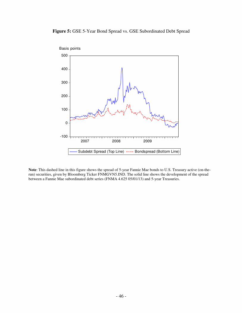
- 46 -

Figure 5: GSE 5-Year Bond Spread vs. GSE Subordinated Debt Spread

-100

0

100

200

300

400

500

2007 2008 2009

Subdebt Spread (Top Line) Bondspread (Bottom Line)

Basis points

Note: This dashed line in this figure shows the spread of 5-year Fannie Mae bonds to U.S. Treasury active (on-the-run) securities, given by Bloomberg Ticker FNMGVN5.IND. The solid line shows the development of the spread between a Fannie Mae subordinated debt series (FNMA 4.625 05/01/13) and 5-year Treasuries.

- 47 -

Figure 6: Residual Analysis of Swap-OAS

-40

-20

0

20

40

60

-40

0

40

80

120

2007 2008 2009

Residuals (Left Axis)Swap-OAS (Right Axis)Predicted Swap-OAS (Right Axis)

Note: The swap-OAS line is the Bloomberg Series NOASFNCL.IND. The predicted swap-OAS line shows the predicted values of a regression: OASt = α + β1 * GSE_Spreadt + εt, where the GSE_Spread series is given by the spread between 5-year Fannie Mae bonds and U.S. Treasury active (on-the-run) securities (Bloomberg Series: FNMGVN5.IND). The residual series plots the residuals from the regression.

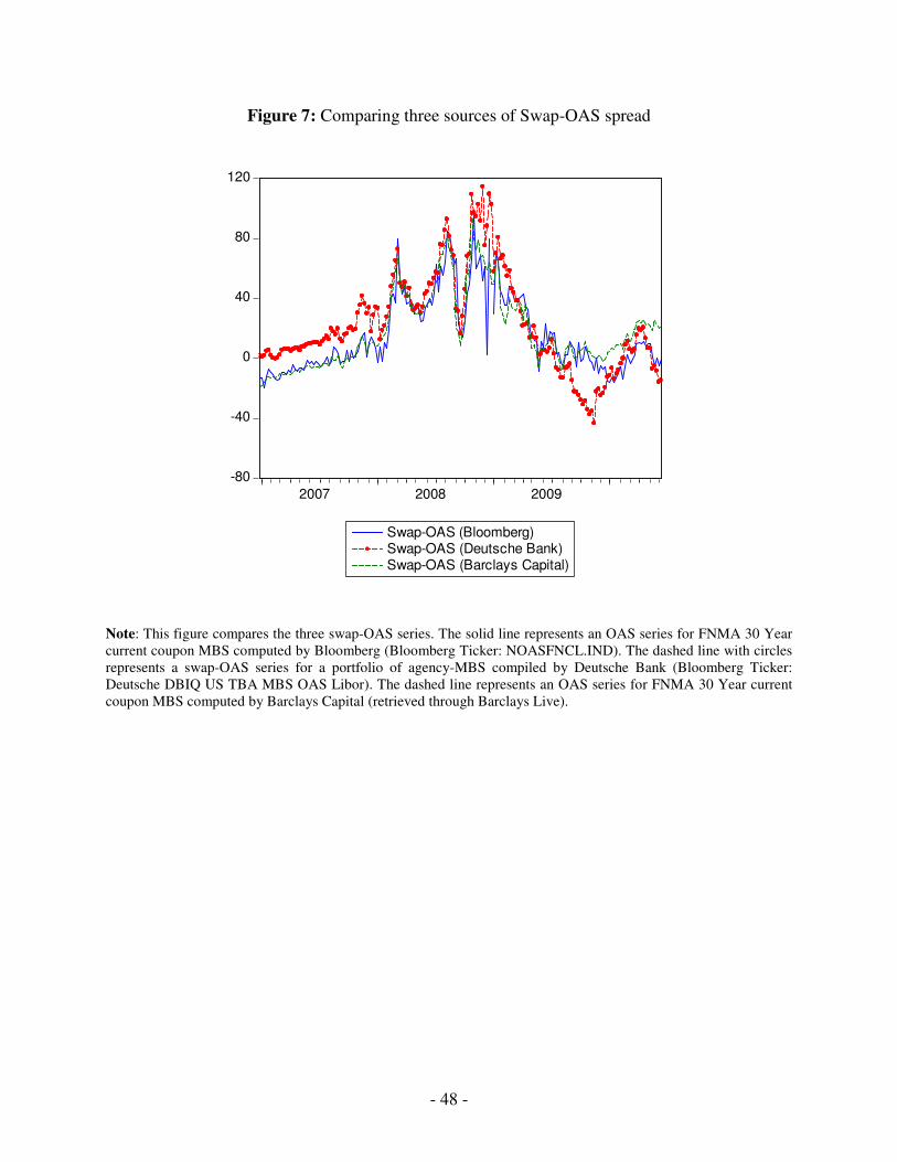
- 48 -

Figure 7: Comparing three sources of Swap-OAS spread

-80

-40

0

40

80

120

2007 2008 2009

Swap-OAS (Bloomberg)Swap-OAS (Deutsche Bank)Swap-OAS (Barclays Capital)

Note: This figure compares the three swap-OAS series. The solid line represents an OAS series for FNMA 30 Year current coupon MBS computed by Bloomberg (Bloomberg Ticker: NOASFNCL.IND). The dashed line with circles represents a swap-OAS series for a portfolio of agency-MBS compiled by Deutsche Bank (Bloomberg Ticker: Deutsche DBIQ US TBA MBS OAS Libor). The dashed line represents an OAS series for FNMA 30 Year current coupon MBS computed by Barclays Capital (retrieved through Barclays Live).

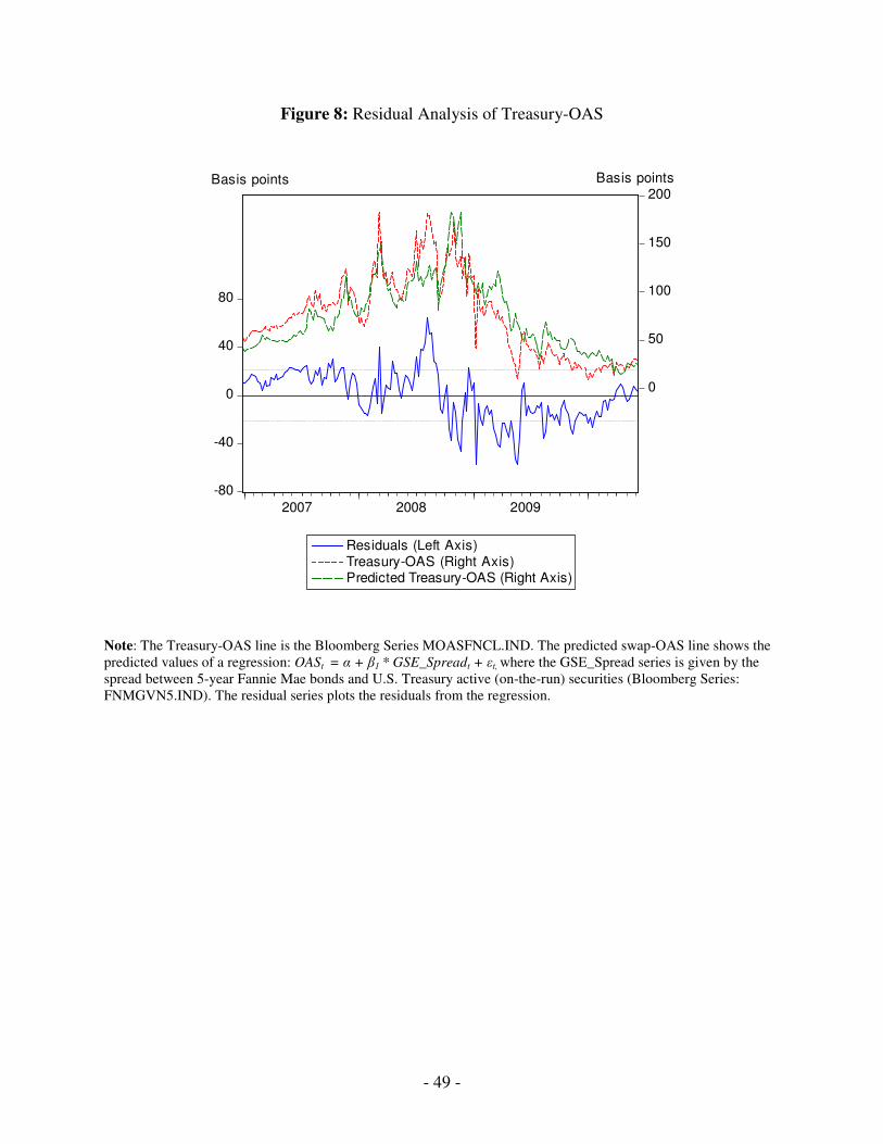
- 49 -

Figure 8: Residual Analysis of Treasury-OAS

-80

-40

0

40

80

0

50

100

150

200

2007 2008 2009

Residuals (Left Axis)Treasury-OAS (Right Axis)Predicted Treasury-OAS (Right Axis)

Basis points Basis points

Note: The Treasury-OAS line is the Bloomberg Series MOASFNCL.IND. The predicted swap-OAS line shows the predicted values of a regression: OASt = α + β1 * GSE_Spreadt + εt, where the GSE_Spread series is given by the spread between 5-year Fannie Mae bonds and U.S. Treasury active (on-the-run) securities (Bloomberg Series: FNMGVN5.IND). The residual series plots the residuals from the regression.

- 50 -

Figure 9: Weekly averages of the 10-Year Swap Spread

-0.2

0.0

0.2

0.4

0.6

0.8

1.0

2007 2008 2009

Percent

Note: This figure shows weekly averages of the difference between the 10-year swap-rate and the 10-year constant maturity Treasury rate. The vertical line is drawn for the week ended November 15, 2008.

- 51 -

Figure 10: Daily Observations on the 10-Year Swap Spread in Late 2008

.0

.1

.2

.3

.4

.5

.6

.7

.8

1 Sep

15 S

ep

29 S

ep

13 O

ct

27 O

ct

10 N

ov

24 N

ov

8 Dec

Oct 3

/

/

Nov 25

Percent

Note: This figure shows daily observations on the difference between the 10-year swap-rate and the 10-year

constant maturity Treasury rate.

Estimated Impact of the Fed's Mortgage-Backed...

Documents

Transcript of Estimated Impact of the Fed's Mortgage-Backed...