NASA/TM-1999-206586

Estimated Benefits of Variable-Geometry Wing Camber Control for Transport Aircraft

Alexander BolonkinSenior Research Associate of the National Research CouncilDryden Flight Research CenterEdwards, California

Glenn B. GilyardDryden Flight Research CenterEdwards, California

October 1999

The NASA STI Program Office . . . in Profile

Since its founding, NASA has been dedicatedto the advancement of aeronautics and space science. The NASA Scientific and Technical Information (STI) Program Office plays a keypart in helping NASA maintain thisimportant role.

The NASA STI Program Office is operated byLangley Research Center, the lead center forNASA’s scientific and technical information.The NASA STI Program Office provides access to the NASA STI Database, the largest collectionof aeronautical and space science STI in theworld. The Program Office is also NASA’s institutional mechanism for disseminating theresults of its research and development activities. These results are published by NASA in theNASA STI Report Series, which includes the following report types:

• TECHNICAL PUBLICATION. Reports of completed research or a major significantphase of research that present the results of NASA programs and include extensive dataor theoretical analysis. Includes compilations of significant scientific and technical data and information deemed to be of continuing reference value. NASA’s counterpart of peer-reviewed formal professional papers but has less stringent limitations on manuscriptlength and extent of graphic presentations.

• TECHNICAL MEMORANDUM. Scientificand technical findings that are preliminary orof specialized interest, e.g., quick releasereports, working papers, and bibliographiesthat contain minimal annotation. Does notcontain extensive analysis.

• CONTRACTOR REPORT. Scientific and technical findings by NASA-sponsored contractors and grantees.

• CONFERENCE PUBLICATION. Collected papers from scientific andtechnical conferences, symposia, seminars,or other meetings sponsored or cosponsoredby NASA.

• SPECIAL PUBLICATION. Scientific,technical, or historical information fromNASA programs, projects, and mission,often concerned with subjects havingsubstantial public interest.

• TECHNICAL TRANSLATION. English- language translations of foreign scientific and technical material pertinent toNASA’s mission.

Specialized services that complement the STIProgram Office’s diverse offerings include creating custom thesauri, building customizeddatabases, organizing and publishing researchresults . . . even providing videos.

For more information about the NASA STIProgram Office, see the following:

• Access the NASA STI Program Home Pageat

http://www.sti.nasa.gov

• E-mail your question via the Internet to help@sti.nasa.gov

• Fax your question to the NASA Access HelpDesk at (301) 621-0134

• Telephone the NASA Access Help Desk at(301) 621-0390

• Write to:NASA Access Help DeskNASA Center for AeroSpace Information7121 Standard DriveHanover, MD 21076-1320

NASA/TM-1999-206586

Estimated Benefits of Variable-Geometry Wing Camber Control for Transport Aircraft

Alexander BolonkinSenior Research Associate of the National Research CouncilDryden Flight Research CenterEdwards, California

Glenn B. GilyardDryden Flight Research CenterEdwards, California

October 1999

National Aeronautics andSpace Administration

Dryden Flight Research CenterEdwards, California 93523-0273

NOTICE

Use of trade names or names of manufacturers in this document does not constitute an official endorsementof such products or manufacturers, either expressed or implied, by the National Aeronautics andSpace Administration.

Available from the following:

NASA Center for AeroSpace Information (CASI) National Technical Information Service (NTIS)7121 Standard Drive 5285 Port Royal RoadHanover, MD 21076-1320 Springfield, VA 22161-2171(301) 621-0390 (703) 487-4650

4

. 5. . . 5. . . . . 7 . . . 8. . .

. . 10

11

.

. . 14

CONTENTS

Page

ABSTRACT . . . . . . . . . . . . . . . . . . . . . . . . . . . . . . . . . . . . . . . . . . . . . . . . . . . . . . . . . . . . . . . . . . . . . . . 1

NOMENCLATURE . . . . . . . . . . . . . . . . . . . . . . . . . . . . . . . . . . . . . . . . . . . . . . . . . . . . . . . . . . . . . . . . . 1Symbols . . . . . . . . . . . . . . . . . . . . . . . . . . . . . . . . . . . . . . . . . . . . . . . . . . . . . . . . . . . . . . . . . . . . . . . 1Subscripts . . . . . . . . . . . . . . . . . . . . . . . . . . . . . . . . . . . . . . . . . . . . . . . . . . . . . . . . . . . . . . . . . . . . . 3

INTRODUCTION . . . . . . . . . . . . . . . . . . . . . . . . . . . . . . . . . . . . . . . . . . . . . . . . . . . . . . . . . . . . . . . . . . 3

WING CAMBER CONTROL BACKGROUND. . . . . . . . . . . . . . . . . . . . . . . . . . . . . . . . . . . . . . . . . .

ANALYTICAL DEVELOPMENT OF VARIABLE-GEOMETRYWING CAMBER OPTIMIZATION . . . . . . . . . . . . . . . . . . . . . . . . . . . . . . . . . . . . . . . . . . . . . . . .Development of Low-Speed Lift and Drag Coefficient Expressions as a Function of Camber. . Influence of Shape on Aerodynamics . . . . . . . . . . . . . . . . . . . . . . . . . . . . . . . . . . . . . . . . . . . . . . . 6Influence of Mach Number on Aerodynamics . . . . . . . . . . . . . . . . . . . . . . . . . . . . . . . . . . . . . . .Influence of Pitching Moments on Aerodynamics . . . . . . . . . . . . . . . . . . . . . . . . . . . . . . . . . . . .General Correction for Nonparabolic Polar . . . . . . . . . . . . . . . . . . . . . . . . . . . . . . . . . . . . . . . . . 9Summary of Equations . . . . . . . . . . . . . . . . . . . . . . . . . . . . . . . . . . . . . . . . . . . . . . . . . . . . . . . . . . . . 9Influence of the Lift-to-Drag Ratio on Fuel Consumption . . . . . . . . . . . . . . . . . . . . . . . . . . . . .

CALCULATION OF VARIABLE-CAMBER BENEFITS FORA TYPICAL WIDE-BODY TRANSPORT . . . . . . . . . . . . . . . . . . . . . . . . . . . . . . . . . . . . . . . . . . .Database Development . . . . . . . . . . . . . . . . . . . . . . . . . . . . . . . . . . . . . . . . . . . . . . . . . . . . . . . . . . 11

. . . . . . . . . . . . . . . . . . . . . . . . . . . . . . . . . . . . . . . . . . . . . . . . . . . . . . . . . . . . . . . . . . . . . . . 12. . . . . . . . . . . . . . . . . . . . . . . . . . . . . . . . . . . . . . . . . . . . . . . . . . . . . . . . . . . . . . . . 12

. . . . . . . . . . . . . . . . . . . . . . . . . . . . . . . . . . . . . . . . . . . . . . . . . . . . . . . . . . . . . . . . . . . . 12 . . . . . . . . . . . . . . . . . . . . . . . . . . . . . . . . . . . . . . . . . . . . . . . . . . . . . . . . . . . . . . . . . . . . . . . 13

. . . . . . . . . . . . . . . . . . . . . . . . . . . . . . . . . . . . . . . . . . . . . . . . . . . . . . . . . . . . . . . . . . . 13. . . . . . . . . . . . . . . . . . . . . . . . . . . . . . . . . . . . . . . . . . . . . . . . . . . . . . . . . . . . . . . . . . . . . 13 . . . . . . . . . . . . . . . . . . . . . . . . . . . . . . . . . . . . . . . . . . . . . . . . . . . . . . . . . . . . . . . . . . . . . 14

Calculation of Variable-Camber Benefit from Database . . . . . . . . . . . . . . . . . . . . . . . . . . . . . . .

ESTIMATED BENEFITS OF VARIABLE CAMBER FOR THE L-1011 EXAMPLE . . . . . . . . . . . 14Low-Speed Flight (Mach 0.60) . . . . . . . . . . . . . . . . . . . . . . . . . . . . . . . . . . . . . . . . . . . . . . . . . . . . 14Cruise Flight (Mach 0.83). . . . . . . . . . . . . . . . . . . . . . . . . . . . . . . . . . . . . . . . . . . . . . . . . . . . . . . . . 15Application of Variable Camber . . . . . . . . . . . . . . . . . . . . . . . . . . . . . . . . . . . . . . . . . . . . . . . . . . . 15

CONCLUDING REMARKS . . . . . . . . . . . . . . . . . . . . . . . . . . . . . . . . . . . . . . . . . . . . . . . . . . . . . . . . . 16

REFERENCES . . . . . . . . . . . . . . . . . . . . . . . . . . . . . . . . . . . . . . . . . . . . . . . . . . . . . . . . . . . . . . . . . . . 18

CD∆CDmin

δ( )∆CDnpCDi∆CDwave∆CDm∆CDc

iii

. . 20

. . 20

.

. 21

. . 22

. . 22

. 23

. . 2

.

. . 2

. . 2

. .

. . 25

. . 25

. .

. . 27

. . 27

. 28

. . 29

. . 29

. . 30

FIGURES

Page

1. Lift coefficient plotted as a function of angle of attack (schematic).. . . . . . . . . . . . . . . . . . . .

2. Drag coefficient plotted as a function of angle of attack (schematic).. . . . . . . . . . . . . . . . . . .

3. Schematic of a typical polar of an aircraft. . . . . . . . . . . . . . . . . . . . . . . . . . . . . . . . . . . . . . . . . 21

4. Ratio as a function of lift coefficient (schematic) . . . . . . . . . . . . . . . . . . . . . . .

5. Lift coefficient as a function of angle of attack and flap deflection (schematic). . . . . . . . . . .

6. Airplane polar as a function of flap deflection (schematic). . . . . . . . . . . . . . . . . . . . . . . . . . .

7. Typical change in and as a function of (schematic). . . . . . . . . . . . . .

8. Shock formation (schematic). . . . . . . . . . . . . . . . . . . . . . . . . . . . . . . . . . . . . . . . . . . . . . . . . . . . 24

(a) Subsonic flow over entire airfoil.. . . . . . . . . . . . . . . . . . . . . . . . . . . . . . . . . . . . . . . . . . 4

(b) Critical Mach number. . . . . . . . . . . . . . . . . . . . . . . . . . . . . . . . . . . . . . . . . . . . . . . . . . . . 24

(c) Supercritical Mach number.. . . . . . . . . . . . . . . . . . . . . . . . . . . . . . . . . . . . . . . . . . . . . .4

(d) Transonic Mach number. . . . . . . . . . . . . . . . . . . . . . . . . . . . . . . . . . . . . . . . . . . . . . . . .4

9. Influence of trailing-edge deflection on profile pressure distribution andweak shock wave (schematic).. . . . . . . . . . . . . . . . . . . . . . . . . . . . . . . . . . . . . . . . . . . . . . . . . 25

(a) Faired trailing edge . . . . . . . . . . . . . . . . . . . . . . . . . . . . . . . . . . . . . . . . . . . . . .

(b) Trailing-edge-down deflection. . . . . . . . . . . . . . . . . . . . . . . . . . . . . . . . . . . . . . . . . . . .

10. Polar of aircraft for transonic field (schematic). . . . . . . . . . . . . . . . . . . . . . . . . . . . . . . . . . .26

11. Drag coefficients as a function of Mach number and trailing-edge (flap)deflection (schematic). . . . . . . . . . . . . . . . . . . . . . . . . . . . . . . . . . . . . . . . . . . . . . . . . . . . . . . . 26

12. Minimum drag coefficient as a function of Mach number (schematic). . . . . . . . . . . . . . . . .

13. Efficiency factor K as a function of Mach number (schematic) . . . . . . . . . . . . . . . . . . . . . .

14. Wave drag coefficient as a function of Mach number and CL (schematic). . . . . . . . . . . . . . . . 28

15. Variation of wing drag coefficient with Mach number (schematic). . . . . . . . . . . . . . . . . . . . .

16. Polar of airplane as a function of the flap deflection (schematic).. . . . . . . . . . . . . . . . . . . . .

17. Variation of drag polar as a function of trailing-edge deflection (schematic). . . . . . . . . . . .

18. The L-1011 airplane. . . . . . . . . . . . . . . . . . . . . . . . . . . . . . . . . . . . . . . . . . . . . . . . . . . . . . . . . . 30

19. Real and parabolic polar of the L-1011 airplane for Mach 0.60 and Mach 0.83. . . . . . . . . .

E CL CD⁄=

∆CLmaxδ( ) ∆CLo

δ( ) δ

δ 0=( )

iv

. .

. 31

. 32

. 32

.

.

. . . 35

6

. 36

. . 37

. . 37

. 38

. 38

. . 39

. . 39

Page

20. Decrement of minimum drag coefficient as a function of trailing-edge (flap)deflection.. . . . . . . . . . . . . . . . . . . . . . . . . . . . . . . . . . . . . . . . . . . . . . . . . . . . . . . . . . . . . . . . . . 31

21. Nonparabolic variation of drag coefficient. . . . . . . . . . . . . . . . . . . . . . . . . . . . . . . . . . . . . . .31

(a) Decrement of drag coefficient . . . . . . . . . . . . . . . . . . . . . . . . . . . . . . . . .

(b) Decrement of drag coefficient as a function of trailing-edge (flap) deflection. . . . . . . .

22. Decrement of the lift coefficient as a function of the trailing-edge (flap) deflection. . . . . . . .

23. Increment of wave drag coefficient as a function of the lift coefficient and Machnumber. . . . . . . . . . . . . . . . . . . . . . . . . . . . . . . . . . . . . . . . . . . . . . . . . . . . . . . . . . . . . . . . . . . . 33

24. Increment of the critical lift coefficient as a function of Mach number andtrailing-edge (flap) deflection. . . . . . . . . . . . . . . . . . . . . . . . . . . . . . . . . . . . . . . . . . . . . . . . . . . 33

25. Incremental pitching moment from variable camber (flat-plate flap) fromtypical airfoil (NASA 23012). . . . . . . . . . . . . . . . . . . . . . . . . . . . . . . . . . . . . . . . . . . . . . . . . .. 34

26. Correction on real polar for Mach 0.60.. . . . . . . . . . . . . . . . . . . . . . . . . . . . . . . . . . . . . . . . .. 34

27. Correction on real polar for Mach 0.83.. . . . . . . . . . . . . . . . . . . . . . . . . . . . . . . . . . . . . . . . .. 35

28. A family of polars of the L-1011 aircraft with variable camber for different deflectionof trailing-edge angles and Mach 0.60. . . . . . . . . . . . . . . . . . . . . . . . . . . . . . . . . . . . . . . . .

29. Relation of variation with CL for a range of trailing-edge deflections. . . . . . . . . . . . . . . 3

30. Incremental performance benefit variation with trailing-edge deflections. . . . . . . . .

31. Maximum increment of benefit at Mach 0.60. . . . . . . . . . . . . . . . . . . . . . . . . . . . . .

32. Optimal angle of trailing edge at Mach 0.60 (outer locus of fig. 30). . . . . . . . . . . . . . . . . . .

33. A family of polars for different deflections of trailing-edge angles at Mach 0.83. . . . . . . . . .

34. Relation for different flap deflections at Mach 0.83. . . . . . . . . . . . . . . . . . . . .

35. Increment (percent) for different flap deflection at Mach 0.83. . . . . . . . . . . . . . . . . . . .

36. Maximum increment benefit at Mach 0.83. . . . . . . . . . . . . . . . . . . . . . . . . . . . . . . .

37. Optimal angle of trailing edge.. . . . . . . . . . . . . . . . . . . . . . . . . . . . . . . . . . . . . . . . . . . . . . . . . . 40

CLmaxCL–( )

L D⁄

∆L D⁄

∆L D⁄

E CL CD⁄=

∆E

∆L D⁄

v

Usingaces ofat if all

t most usesost

affectn thisd wind-urfaceed forfor are thanrcent.

ABSTRACT

Analytical benefits of variable-camber capability on subsonic transport aircraft are explored. aerodynamic performance models, including drag as a function of deflection angle for control surfinterest, optimal performance benefits of variable camber are calculated. Results demonstrate thwing trailing-edge surfaces are available for optimization, drag can be significantly reduced apoints within the flight envelope. The optimization approach developed and illustrated for flightvariable camber for optimization of aerodynamic efficiency (maximizing the lift-to-drag ratio). Mtransport aircraft have significant latent capability in this area. Wing camber control that can performance optimization for transport aircraft includes symmetric use of ailerons and flaps. Ipaper, drag characteristics for aileron and flap deflections are computed based on analytical antunnel data. All calculations based on predictions for the subject aircraft and the optimal sdeflection are obtained by simple interpolation for given conditions. An algorithm is also presentcomputation of optimal surface deflection for given conditions. Benefits of variable camber transport configuration using a simple trailing-edge control surface system can approach mo10 percent, especially for nonstandard flight conditions. In the cruise regime, the benefit is 1–3 pe

NOMENCLATURE

Symbols

mean aerodynamic chord, ft

specific fuel consumption, min–1

drag coefficient

analytical drag coefficient in a given area

induced drag coefficient

balance drag

relative balance drag,

for

for

drag coefficient from wind-tunnel test

aircraft lift coefficient

maximum wing lift coefficient

for

for

minimum wing lift coefficient

lift coefficient in point

for

pitching-moment coefficient

c

c1

CD

CDanalytical

CDi

CDm

CDmCDm

CD⁄

CDminδ( ) CDmin

δ 0≠

CDminδ 0=( ) CDmin

δ 0=

CDtest

CL

CLmax

CLmaxδ( ) CLmax

δ 0≠

CLmaxδ 0=( ) CLmax

δ 0=

CLmin

CLoCDmin

CLoδ 0=( ) CLo

δ 0=

Cm

r

pressure coefficient

D drag force, lbf

E aerodynamic efficiency

change in E, percent

ratio of to for

K efficiency factor in formula of induced drag

L lift force, lbf

lift-to-drag ratio

M Mach number

critical Mach number

free-stream Mach number

air pressure in given point, lbf/ft2

free-stream static pressure, lbf/ft2

q dynamic pressure, lbf/ft2

Re Reynolds number

S wing platform area, ft2

St stabilizer platform area, ft2

T thrust, lbf

W gross weight, lb

fuel consumption rate, lb/min

change in fuel consumption, percent

x distance from leading edge, ft

X distance between the wing and stabilizer, ft

angle of attack, deg

flap angle or deflection of trailing edge (positive is down), deg

change

correction of parabolic polar

increment of between parabolic variation and nonparabolic variation fo

high and low lift coefficients

increment of for region near

increment of for region near

additional wave drag coefficient for

change of coefficient in point from angle of trailing edge

Cp

E L D⁄ CL CD⁄= =( )

E

Eo CL CD δ 0=

L D⁄

Mcr

M∞p

p∞

wf

wf

c 4⁄( ) c 4⁄( )

α

δ

∆

∆CDc

∆CDnpCD

∆CDnpLmaxCD CLmax

∆CDnpLminCD CLmin

∆CDwaveM Mcr>( )

∆CLoδ( ) CLo

CDmin

2

ent ofction of

s canecauseoff andariable-ults inmental

meansircraftof thisnt- andboard

W) cruiseehile

cludedmber

0/340ms

change in where wave drag appears

additional pitching moment from trailing edge

Subscripts

max maximum

min minimum

opt optimum

t horizontal tail

wing wing

INTRODUCTION

Aircraft efficiency is an important factor for airline operation. Fuel costs can approach 50 percairline operating expense for some modern, wide-body, long-range transports. A 3-percent redufuel consumption can produce savings of as much as $300,000/yr for each aircraft.1 Variable-cambercontrol of the wing for drag reduction throughout the flight mission using existing control surfaceprovide the ability to realize these savings. Variable camber is ideally suited for future aircraft bthe available control surfaces can be used throughout the flight envelope: flaps used for takelanding and ailerons used for routine turning maneuvers can be used in combination to provide vcamber control during cruise flight. In addition to these savings, reduced fuel consumption resequivalent reductions in atmospheric gas emissions, which is an increasingly important environissue.

Many issues enter into performance optimization for transport aircraft.2–5 Foremost, the potential foroptimization must exist, which implies redundant control effect capability (that is, more than one of trimming the forces and moments to obtain a steady-state flight condition). Most transport ahave significant capability in this area; taking maximum advantage of this capability is the theme paper. Controls and variables that potentially can play a role in performance optimization for currefuture-generation transport aircraft include the elevator, horizontal stabilizer, outboard aileron, inaileron, flaps, slats, rudder, center of gravity, and differential thrust.

The Advanced Fighter Technology Integration (AFTI)/F-111 Mission Adaptive Wing (MAprogram developed and demonstrated the potential of using variable-camber control to optimizeand maneuver flight conditions for fighter configurations.6, 7 In general, the objective was to have thability to actively modify airfoil camber, spanwise camber distribution, and wing sweep in flight wmaintaining a smooth and continuous airfoil surface. Features of the mission adaptive wing incruise camber control to maximize vehicle efficiency during straight and level flight; maneuver cacontrol; maneuver load control; and maneuver enhancement and gust alleviation.

Preliminary design work has been performed for implementing variable camber into the A-33transport and other aircraft.2 In addition, numerous reports document trajectory optimization algorithand their benefits relative to the economics of commercial transports.4, 5 In fact, all large transports

∆CLwaveCL

∆M

3

jectoryeion; no

uctionnsportde theriable- applied.

ementequire

sonice dragizationraftdictedd flap

s theg- andever, is a full-

of flapamongntrolns in

provideabilizer,

urrent-ariablebenefitsriable-

currently being produced have onboard flight management systems that “optimize” the aircraft trato minimize cost as a function of flight time and fuel price.8 However, the commonality of all thesalgorithms is that the model used for performance optimization is the predicted base configuratability exists to use variable-geometry features that are available with redundant control surfaces.

NASA Dryden Flight Research Center (Edwards, California) has developed drag-redtechnologies for transport aircraft. The realizable performance benefits typically are smaller for traaircraft than for fighter aircraft, and as such, the task is challenging. These technologies incluapplication of measurement-based optimum control for performance improvement using vageometry concepts (redundant control effects). For example, symmetric aileron deflection can beto optimally recamber the wing to minimize drag for all aircraft configurations and flight conditions1

For fly-by-wire transports, the modification can be as simple as loading new flight managsystem and control display unit software. Transport aircraft with mechanical systems additionally rrelatively simple control hardware modifications.

This analytical study explores the potential benefits of variable-camber capability on subtransport aircraft. Using aerodynamic performance models of the aircraft, including control-surfaceffects, optimum performance benefits of variable camber can be calculated. The optim(maximizing the lift-to-drag ratio, ) typically is minimization of aircraft drag for various aircconfigurations and flight conditions. This paper presents a method for computing optimally presurface deflection for given flight conditions and predicted drag characteristics for aileron andeflections based on analytical and wind-tunnel data.

WING CAMBER CONTROL BACKGROUND

The Wright brothers’ attempt to alter lift characteristics using wing warping may be viewed afirst practical application of varying camber. Subsequent aircraft designs have employed leadintrailing-edge devices to improve low-speed takeoff and landing performance. The challenge, howto include cruise flight in the variable-camber concept in order to maximize the benefits of havingenvelope variable-camber capability.1–3

Current subsonic-transport design results in a point-design configuration with the exception usage at low-speed flight conditions. By necessity, the final configuration is a major compromise a multitude of design considerations. Additional operational constraints include air-traffic-codirectives (speed and altitude), loading (cargo and fuel), center of gravity, flight length, variatiomanufacturing, aging, and asymmetries.3

Current-generation aircraft have a wide range of control surfaces that can be adapted to varying degrees of variable-camber capability. These surfaces include the elevator, horizontal stoutboard aileron, inboard aileron, outboard flaps, and inboard flaps.

Mechanical and software changes would be required to implement variable camber in cgeneration aircraft, and some surfaces are significantly simpler to use than others. Ideally, vcamber should be designed into the aircraft rather than retrofitted. Such a design would have because the aerodynamic tailoring would be optimized for application of variable camber. A vacamber aircraft will be modestly more complex than current-generation aircraft.6, 7, 9, 10

L D⁄

4

ansport for lifttion ofwing the

wingfound

regionbolic

cruise

e the

ANALYTICAL DEVELOPMENT OF VARIABLE-GEOMETRYWING CAMBER OPTIMIZATION

The equations describing the influence of camber in the calculated performance of a generic-trwing profile are developed based on theoretical concepts and wind-tunnel data. The equationsand drag coefficients are expanded to include all effects for a typical transport wing. The applicathe variable-camber feature is noted as the development progresses. Emphasis is placed on shoeffects of variable camber.

Development of Low-Speed Lift and Drag Coefficient Expressionsas a Function of Camber

Aircraft lift coefficient and drag coefficient can be defined as

(1)

and

(2)

Lift and drag coefficients are complex functions of profile shape, angle of attack , planform (S), Mach number (M), Reynolds number (Re), and so forth. These functions may be from computation, wind-tunnel testing, or flight testing.

The aerodynamic results are typically presented as graphs of

(3)

(4)

and

(5)

Figures 1–3 show typical variations of these functions for low-speed (no shock wave) flight. In the where the CL variation with is approximately linear, the curves of equations (4) and (5) have parashape. A very important characteristic of transport aircraft is the maximum achievable in flight,

, (6)

which figure 4 shows as a function of The objective of performance optimization is to maximiz at all cruise flight conditions.

CL( ) CD( )

CL L q⁄ S =

CD D qS⁄ .=

α( )

CL f α( ),=

CD f α( ),=

CD f CL( ).=

αL D⁄

L D⁄ CL CD⁄=

CL.L D⁄

5

be

, K

esting.

ion for

In the

a fixed

For low speed (less than Mach 0.6), the formula of CD can be approximated by

, (7)

where is the minimum of and is drag induced by the lift force. The can

approximated by

, (8)

where is the lift coefficient in point (fig. 3), and K is the efficiency factor. In particular

depends on the aspect ratio of the wing and Mach number.

Outside of the parabolic region, the nonparabolic variations can be found using wind-tunnel tAn expression for over the full range of is:

, (9)

where is the increment of between the parabolic variation and the nonparabolic variat

high and low lift coefficients—in other words, the increment of CD in regions near and

(figs. 1 and 3):

(10)

or

. (11)

Influence of Shape on Aerodynamics

The wing trailing edge has a strong influence on the aerodynamics of a given wing profile.

subsonic region, increasing camber (increasing downward flap deflection, ) requires less for

CL, or increases the coefficient CL for a constant (fig. 5).11 The linear region of CL as a function of

is also increased to a larger CL. The maximum CL also increases (fig. 5):

. (12)

The coefficient increases (fig. 6) by the relation

. (13)

CD CDminCDi

+=

CDminCD, CDi

CDi

CDiK CL CLo

–( )2=

CLoCDmin

CD CL

CD CDminCDi

∆CDnpCL( )+ +=

∆CDnpCD

CLmaxCLmin

∆CDnp∆CDnpLmax

=

∆CDnp∆CDnpLmin

=

δ αα α

CLmaxδ( ) CLmax

δ 0=( ) ∆CLmaxδ( )+=

CDmin

CDminδ( ) CDmin

δ 0=( ) ∆CDminδ( )+=

6

. 6).

ypical

upperumbernd, theweenf flow

rofile, the

camber

l

lift from wavem an

ng

The flap deflection changes the lift coefficient for minimum drag by the amount (figThe coefficient equals

, (14)

where is the change in caused by trailing-edge deflection (fig. 6). Figure 7 shows t

variations of the and as a function of .

Influence of Mach Number on Aerodynamics

For high-speed (transonic) flight (Mach 0.6–0.9), development of a normal shock wave on theairfoil surface results in additional drag effects (fig. 8). At speeds faster than the critical Mach n

, where the velocity of certain regions on the upper surface reach the speed of soucoefficients CL, CD, and K also depend on Mach number. The critical Mach number, typically betMach 0.6 and 0.8, depends on the airfoil profile and the position of the profile to the direction o(angle of attack of the wing).

Camber or flap deflection also influences the critical Mach number. A nonsupercritical p(without flap deflection) may incur supercritical properties with a slight flap deflection. In this casepressure coefficient (Cp) distribution of the surface profile is changed (fig. 9):

. (15)

The maximum Cp is decreased and a strong shock wave becomes a weak shock wave for small increases. As a result, the critical Mach number increases.

When the Mach number is greater than the critical Mach number, CD increases by the additionawave drag increment, (fig. 10).

(16)

The depends on the CL of the wing in the transonic speed regime. For small coefficients, figure 10 shows the drag form is approximately parabolic in the transonic rangepoint A to point B. For lift coefficients greater than point B at transonic speeds, a normal shockdevelops that produces an additional wave drag component [ , which departs froapproximately parabolic curve (fig. 10) when the ]. After addiequations (13) and (16), equation (9) now has a form

. (17)

For , the point where departs from a parabola is increased by the value

. (18)

CLo∆CLo

δ( )CLo

CLoδ( ) CLo

δ 0=( ) ∆CLoδ( )+=

∆CLoδ( ) CLo

∆CLoδ( ) ∆CLmax

δ( ) δ

Mcr( )

Cp p p∞–( ) q⁄=

∆CDwave

∆CDwave∆CDwave

CL ∆CLwaveM δ,( )–( ) M,( )=

∆CDwaveα( )

CD f CL( )=CL is greater than point B

CD CDminCDi

∆CDnp∆CDmin

∆CDwave+ + + +=

δ 0> CD f CL( )=

∆CLwave∆CLwave

M δ,( )=

7

gion of

f M

cts thatmally at theering.. Thell thus

camber

by an

Note that the break from parabolic shape caused by the shock wave can occur in the linear re.

Figures 11–16 show typical variations of , , K, , and as a function o

and . Figure 17 shows typical polars as a function of .

Influence of Pitching Moments on Aerodynamics

The cambering effects, discussed in previous sections, also introduce pitching-moment efferequire aircraft retrimming using the horizontal tail. A positive increase in camber on the wing norproduces a negative pitching moment, which in turn must be balanced by a negative lift forcehorizontal tail that produces a moment tending to cancel the moment from the wing cambConsequently, the wing must produce an additional positive lift force for a fixed weight conditionadditional positive lift force produces additional induced drag. The benefit from variable camber widecrease.

An estimate of the effects that pitching moments have on the performance benefits of variable is derived as follows: The additional pitching moment caused by flap deflection is

, (19)

where is the pitching-moment coefficient increment. This moment must be balanced additional moment of horizontal tail,

, (20)

where the tail lift force is

(21)

and X is the distance between the wing and stabilizer.

Setting equations (19) and (20) equal,

. (22)

The increase in wing lift can be expressed as

. (23)

Summing equations (21) and (23) and setting them equal to 0 yields

. (24)

CL α( )

CD CDmin∆CLwave

∆CDwaveMcr δ

∆M ∆CmqSc=

∆Cm

∆Mt ∆LtX ∆CLtqStX = =

∆Lt ∆CLtqSt =

c 4⁄( ) c 4⁄( )

∆CLt∆CmSc StX( )⁄=

∆Lwing ∆CLqS=

∆CL ∆CLtSt– S⁄=

8

change,

urring. If polar,he wind-

7),

Because the induced drag coefficient of the wing is

,

the incremental drag coefficient caused by pitching-moment effects is

.

Simplifying the above yields

. (25)

Substituting equation (22) into equation (24) produces

. (26)

Substituting equation (26) into equation (25) produces

. (27)

This term then is added to the previous drag expression of equation (18). The percentage of drag, of to the of equation (18) is

(28)

General Correction for Nonparabolic Polar

The drag equation development has assumed a parabolic shape to the point of wave drag occwind-tunnel data are available in the region of low lift coefficients and indicate a nonparabolic draga correction term can be added for the difference between the assumed parabolic shape and ttunnel data (fig. 3). This correction term can be expressed as

. (29)

Summary of Equations

Summarizing the derivation of CD by substituting the terms from equations (9)–(11), (16), (17), (2and (29), the aircraft drag coefficient can be rewritten as:

(30)

CDiK CL CLo

–( )2=

∆CDmCDi

with flaps( ) CDino flaps( ) K CL ∆CL CLo

–+( )2K CL CLo

–( )2–=–=

∆CDmK 2∆CL CL CLo

–( ) ∆CL2+[ ]=

∆CL ∆Cmc– X⁄=

∆CDmK 2∆Cm CL CLo

–( )c X⁄– ∆Cmc X⁄( )2+=

∆CDm∆CDm

CD

∆CDm∆CDm

CD⁄( ) 100 percent.⋅=

∆CDc∆CDc

CL( )=

CD CDminδ 0=( ) ∆CDmin

δ( ) ∆CDnpCL δ,( ) CDi

CL CLoδ( ) M,,( )+ + +=

∆CDwaveCL ∆CLwave

M δ,( )– M,[ ] ∆ CDmCL δ,( ) ∆CDc

CL( ).+ ++

9

is

the

hich

and

uel

is the total drag, is the minimum of drag coefficient (figs. 2 and 3), and

the increment minimum drag coefficient from flap (eq. (13) and fig. 6).

,

where is the increment in region (eq. (10)) and , is

increment in the region (eq. (11) and fig. 3).

, the induced drag coefficient (eqs. (8) and (14) and fig. 3), is

, (31)

where is the efficiency coefficient (eq. (8)); and is the change coefficient , w

depends on the angle of deflection, (fig. 6).

is the increment of drag coefficient from (M, ) in equation (16).

is the increment of lift coefficient from change pressure distribution (eq. (16)fig. 16).

, (32)

and is the correction of the parabolic polar to the real polar for a few lift coefficients.

Influence of the Lift-to-Drag Ratio on Fuel Consumption

Fuel consumption is proportional to the aircraft total thrust:

, (33)

where is the fuel consumption rate, T is the thrust of all airplane engines, and is the specific fconsumption and is assumed constant at cruise conditions. At stabilized cruise conditions,

. (34)

CD CDminδ 0=( ) ∆CDmin

δ( )

∆CDnp∆CDnpLmax

CL( ) ∆CDnpLminCL δ,( )+=

∆CDnpLmaxCL( ) CD CLmax

∆CDnpLminCL δ,( )

CD CLmin

CDi

CDiK M( ) CL CLo

δ 0=( )– ∆CLoδ( )–( )2⋅=

K M( ) ∆CLoδ( ) CLo

δ

∆CDwaveCL ∆C–

LwaveM δ,( )( ) M,[ ]

δ

∆CLwaveM δ,( )

∆CDmK 2∆Cm CL CLo

–( )c X⁄– ∆Cmc X⁄( )2+ balance drag (eq. (27)).–=

CLoCLo

δ 0=( ) ∆CLoδ( )+=

∆CDcCL( )

wf c1T=

wf c1

T W E⁄=

10

using

flection,

section

igure 18

ntative

y of the

would be

rms of

eloped in

Substituting equation (34) into equation (33),

, (35)

where . Find :

. (36)

Noting that

(37)

then

(38)

The percent of fuel consumption is related to the percent of the aerodynamic efficiency as

. (39)

CALCULATION OF VARIABLE-CAMBER BENEFITS FORA TYPICAL WIDE-BODY TRANSPORT

As observed from equations (1)–(39), the aerodynamics of a variable-camber configuration

only trailing-edge control surfaces are complex and depend on factors such as trailing-edge de

Mach number, and so forth. This section expands on the theoretical development of the previous

and develops the example database from which the variable-camber benefits can be calculated. F

shows the L-1011 transport (Lockheed Corporation, Burbank, California) selected as a represe

aircraft to demonstrate the benefits of variable camber.

Database Development

This section develops an appropriate database. The available L-1011 data do not contain man

required parameters; thus, these parameters were obtained from other sources. Using flight data

ideal; lacking that, wind-tunnel or analytical data must be used. This section takes the te

equation (30) and discusses the development of the database for each term. The database dev

this section is then used to calculate benefits that will be discussed in the next section.

wf c1W E⁄=

E L D⁄ CL CD⁄= = dwf dE⁄

dwf c1WdE E2⁄–=

dwf dwf wf⁄( ) 100 percent⋅ dwf E c1W⁄( ) 100 percent,⋅= =

dE dE E⁄( ) 100 percent.⋅=

L D⁄

dwf dE–=

11

areure 19

hese

-edge

iques

ed to be

antlyated

imal lift

e as

The term CD is obtained from unpublished L-1011 flight results. For this report, two conditionsanalyzed: Mach 0.60 for climb and descent regimes, and Mach 0.83 for cruise conditions. Figshows polars for these two conditions.

The approximate parabolic region used for this analysis is as follows:

(40)

Assuming a parabolic polar form of

, (41)

a fit of the data (fig. 19) yields values of , K, and for regions defined by equation (40). Tvalues are as follows:

(42)

(43)

Figure 19 also shows the parabolic fits.

The term represents how the minimum drag coefficient varies with respect to trailing

control surface deflection, (fig. 20). The term is calculated based on empirical data and techn10

using a correction for smooth surface and data obtained from reference 12. The term is assum

independent of Mach number.

At extreme values of CL, the actual drag polar begins to deviate and continues to deviate significfrom the ideal parabolic variation (fig. 3). The variations at the extreme lift coefficients are estimbased on empirical data and techniques of reference 10 and are shown in figure 21. For maxcoefficients, is determined:

,

where is obtained from figure 22 and is obtained from a lift curve slop

indicated in figure 1.

CD

Mach 0.60: CL 0.12–0.60=

Mach 0.83: CL 0.12–0.50=

CD CDminK CL CLo

–( )2+=

CDminCLo

Mach 0.60: CDmin0.0165= K 0.0832= CLo

0.12=

Mach 0.83: CDmin0.018= K 0.10547= CLo

0.16=

∆CDminδ( )

∆CDminδ

∆CDnp

CLmaxδ( )

CLmaxδ( ) CLmax

δ 0=( ) ∆CLmaxδ( )+=

∆CLmaxδ( ) CLmax

δ 0=( )

12

urve.

ons.

ter 3 and

lift

13, 15,

rabolic

r and

tion

rence 8,

64–68.

from

The CL of interest is subtracted from ; the (fig. 21(a)) is then obtained from the c

This value is not a function of trailing-edge deflection, and no correction exists for

(fig. 21(a)).

For minimal lift coefficients, the is read directly from figure 21(b) as a function of CL and flap

deflection, . These values were estimated by the method described in reference 10.

is the maximum lift coefficient obtainable with trailing-edge control surface deflecti

This value is calculated by the method described in reference 10 (also refer to reference 13, chap

reference 14). These terms are assumed to be independent of Mach number.

The term represents the induced drag caused by CL (or angle-of-attack) variation:

;

K and are defined in the section. CL is the lift coefficient of interest, and

is the lift contribution caused by increased trailing-edge deflection (fig. 22). This

contribution is calculated by the method described in reference 10 (also see references 9–11,

and 16).

As indicated earlier, the wave drag component is caused by the shock wave affecting the pa

shape of the drag polar. The wave drag correction term as a function of Mach numbe

is obtained from figure 23; as a function of Mach number and flap deflec

is obtained from figure 24. The estimate is based on data in reference 9, pages 398–406; refe

pages 232–236; reference 15, pages 291–302; reference 13, page 107; and reference 11, pages

The drag correction to pitching-moment balancing of the horizontal tail (eq. 27) is:

,

where is obtained from figure 25 as a function of flap deflection. is obtained

reference 10.

CLmax∆CDnp

CLmaxCL 0.1>–

CDnpδ

∆CLmax

CDi

CDi

CDiK CL CLo

δ 0=( ) ∆CLoδ( )––( )2

=

CLoδ 0=( ) CDmin

δ 0=( )∆CLo

δ( )

∆CDwave

CL ∆CLwave–( ) ∆CLwave

∆CDm

∆CDmK 2∆Cm CL CLo

–( )c X⁄– ∆Cmc X⁄( )2+=

∆Cm ∆Cm

13

wind-

26–27

will

cy:

ft, drageasuresmbers: is the

polarsta for C as a

This correction is the difference between the usual quadratic drag polar (eqs. (7) or (41)) andtunnel or flight data and is defined as:

.

Because the L-1011 database represents a combination of wind-tunnel and flight data, figuresshow this correction for Mach 0.60 and Mach 0.83, respectively.

Calculation of Variable-Camber Benefit from Database

With both CL and CD now available, efficiency factors can be calculated. In this analysis, be used as the measure of efficiency and will also be denoted by E:

. (44)

The percentage change of the efficiency ratio is then

, (45)

where at . The maximum efficiency is found by:

. (46)

These calculations result in the optimum trailing-edge (flap) deflection, , for maximum efficien

. (47)

ESTIMATED BENEFITS OF VARIABLE CAMBER FORTHE L-1011 EXAMPLE

Based on equations (1)–(39) and the aerodynamic database developed for the L-1011 aircrapolars as a function of the entire trailing-edge deflection are calculated, and then performance mare determined from these drag polars. The calculations are performed for two Mach nuMach 0.60, representing a climb or an off–design cruise point condition; and Mach 0.83, whichdesign cruise point of the aircraft.

Low-Speed Flight (Mach 0.60)

Figure 28 shows the family of drag polars as a function of flap deflection for Mach 0.60. Thesehave the classic quadratic shape because wave drag is not a factor at this Mach condition. The daLas a function of CD (fig. 28) are then used to develop the variations (fig. 29) that are shown

∆CDc

∆CDcCDtest

CDanalytical–=

L D⁄

E L D⁄ CL CD⁄= =

E E Eo–( ) Eo⁄[ ] 100 percent⋅=

Eo CL CD⁄= δ 0=

Emax maxδ

E CL M δ,,( ) for fixed CL M,=

δopt

δopt f CL M,( )=

L D⁄

14

r thetrongle at

ed tog flap

re ratherption isately

arisonx. The

n Machmber on

iche in

tion.

ttain flap

ber arein fuel

rfaces, reportmajorlly, the

function of CL for a range of flap deflection. Figure 30 shows the percent of change in fovarious flap conditions relative to the 0° flap-deflection condition. Figure 30 shows as a sfunction of both CL and flap deflection; note that essentially no variable-camber benefit is availab

Figure 31 shows the locus of maximal obtainable.

Figure 32 shows the flap deflection required to attain the maximal at a given CL. Thevariation shows that for very low lift coefficients, a negative (trailing-edge-up) deflection is requirattain improvements; whereas at lift coefficients greater than approximately 0.35, increasindeflection is required to attain the maximal as the CL increases. Cruise flight typically is in the CLrange of 0.40–0.50, and as such, the available improvements produced by variable camber amodest and in the range of 1–3 percent. As noted earlier, the percent of reduction in fuel consumapproximately equal to the percent of increase in . The effect was very small (approxim3 percent) of the benefit.

Cruise Flight (Mach 0.83)

Figure 33 shows the family of drag polars as a function of flap deflection for Mach 0.83. Compwith the drag polars of figure 28 reveals the drag polars for Mach 0.83 are much more completransonic polar is more difficult to calculate because the drag has a complex dependency onumber in the transonic regime and the aerodynamic data describing the influence of variable cathe polar are limited. A small, increasing deflection of trailing-edge surfaces at a constant CL candecrease wave drag, thus delaying the increase of wave drag to a higher Mach number (fig. 9).

The data for CL as a function of CD (fig. 33) are used to develop the L/D variations (fig. 34), whare presented as a function of CL for a range of flap deflection. Figure 35 shows the percent of chang

as a function of for various flap conditions relative to the 0° flap-deflection condiFigure 35 shows that essentially no variable-camber benefit is available at CL ≈ 0.35, very similar to thelow-speed case. Figure 36 shows the locus of the maximal as a function of CL; note that the benefitpeaks out at CL ≈ 1.0.

Figure 37 shows the flap deflection required to attain the maximal at a given CL. The variationshows that for very low lift coefficients, a negative (trailing-edge-up) deflection is required to a

improvements; whereas at lift coefficients greater than approximately 0.35, increasingdeflection is required to attain the maximal as the CL increases. Cruise flight typically is in the CLrange of 0.40–0.50, and as such, the available improvements produced by variable camrather modest and in the range of 1–3 percent. As noted earlier, the percent of reduction consumption is approximately equal to the percent of increase in .

Application of Variable Camber

The methodology developed in this report assumes application to aileron-type trailing-edge sueven in the span locations normally occupied by flaps. Although the benefits discussed in thiscould be obtained with software changes in fly-by-wire aircraft for the aileron surfaces, modifications would be required to develop a system to obtain small deflections for the flaps. Idea

L D⁄L D⁄

CL 0.35.≈ L D⁄

L D⁄

L D⁄L D⁄

L D⁄

L D⁄ CDm

L D⁄ CL

L D⁄

L D⁄

L D⁄L D⁄

L D⁄

L D⁄

15

ber isriable-

; can beas. Or,

reasinglue of theases inable totional

rations,surface

ategoryrmance derived-1011

ch the

60 andenefit

aximumfuel

rizontale. Theraft arer largeratinghave a

e fuel report

benefits of variable camber will be maximized with future-generation aircraft in which variable camincluded in the original design. These future designs could include leading-edge control and vacamber features more revolutionary than the simple trailing-edge rotation discussed in this report.

The benefits of optimization using variable camber discussed in this report involve maximizing this effect can then be used in various ways. For example, instead of saving fuel, the missionflown at a faster speed for the same fuel consumption a lesser speed flown without optimization hbecause less fuel is required for the mission, the fuel weight reduction can be exploited by incpayload (and thus, revenue). Because 1 lb of payload can generate as much as 30 times the vacost of 1 lb of fuel, these benefits can be huge. For payload- or range-limited aircraft, small incre

can mean large increases in revenue. The variable-camber benefits are not only appliccommercial transport aircraft but also to military aircraft that quite often have very large operaflight envelopes, thereby increasing the potential for variable-camber benefits.

The concepts developed in this report can also be applied to supersonic transport–type configufighter aircraft, and helicopters. In addition, the technology can be applied to any aerodynamic (propellers, large turbine blades, varieties of sails, and so forth).17–20

CONCLUDING REMARKS

An analytical approach to assessing the potential benefits of variable camber on transport-caircraft has been developed. The methodology uses the lift-to-drag ratio, , as the perfoparameter to be maximized. The aerodynamic model data required for actual calculations can befrom flight test, wind-tunnel, or analytical sources. The methodology was evaluated using the Laerodynamic model, which is representative of the long-range, wide-body transports for whiapplication of variable camber would be most beneficial.

The evaluation of variable-camber benefits was conducted at two Mach numbers, Mach 0.Mach 0.83, and assumed full-span wing trailing-edge deflection capability. At Mach 0.60, the branged from nearly 0 percent at a lift coefficient (CL) of 0.35 to a maximum of 9–12 percent at a CL rangeof 0.8–1.2. At nominal cruise flight conditions, the benefit is 1–3 percent. The higher CL conditions ofclimb and descent may enable obtaining benefits of 4 percent or more.

For Mach 0.83, the benefit is 1–3 percent in the cruise regime. The benefits are greater (a mof 14 percent) in the region CL > 0.8, but this region is not used for cruise flight. The percent of consumption reduction essentially is equal to the percent of increase at a given condition.

The pitching-moment effect on the caused by wing cambering effects and associated hotail trim changes are approximately percent of the variable-camber benefit in cruise regimvariable-camber benefits for nominal flight conditions are rather modest because commercial aircdesigned to be optimized for these nominal conditions. As such, the potential clearly exists fobenefits as the aircraft is operated at conditions further from the nominal profile. Although opeunder such conditions would be rather infrequent for commercial operations, military operations much broader flight envelope; thus, the potential exists for significant benefits.

The benefits resulting from the application of the variable-camber wing can be used to minimizconsumption, maximize speed, maximize loiter time, and so forth. The benefits calculated in this

L D⁄

L D⁄

L D⁄

L D⁄

L D⁄3–

16

ver, theight be

may not exactly duplicate what is seen in flight because of the inexact nature of the process. Howebenefits calculated accurately reflect trends and provide an indication of the type of benefits that mseen.

Dryden Flight Research CenterNational Aeronautics and Space AdministrationEdwards, California, July 13, 1999

17

rch

20,

ic

1

ng

d

ic

REFERENCES

1. Gilyard, Glenn B., Jennifer Georgie, and Joseph S. Barnicki, Flight Test of an AdaptiveConfiguration Optimization System for Transport Aircraft, NASA TM-1999-206569, 1999.

2. Szodruch, J. and R. Hilbig, “Variable Wing Camber for Transport Aircraft,” Progress in AerospaceSciences, vol. 25, 1988, pp. 297–328.

3. Gilyard, Glenn, In-Flight Transport Performance Optimization: An Experimental Flight ReseaProgram and an Operational Scenario, NASA TM-97-206229.

4. Bolonkin, A. A., New Methods of Optimization and Their Applications, Moscow Highest TechnicalUniversity named Bauman, Moscow, 1972.

5. Bolonkin, Alexander and Narendra Khot, “Method for Finding a Global Minimum,” AIAA-94-44Jan. 1994.

6. Phillips, Paul W. and Stephen B. Smith, AFTI/F-111 Mission Adaptive Wing (MAW) AutomatFlight Control System Modes Lift and Drag Characteristics, AFFTC-TR-89-03, May 1989.

7. National Aeronautics and Space Administration, Advanced Fighter Technology Integration F-11Mission Adaptive Wing, NASA CP-3055, 1989.

8. Jenkins, Darryl, ed., The Handbook of Airline Economics, McGraw-Hill, Washington D.C., 1995,pp. 223–234 and 367–378.

9. Ferris, James C., Wind-Tunnel Investigation of a Variable Camber and Twist Wi,NASA TN-D-8475, 1977.

10. Air Force Flight Dynamics Laboratory, Flight Control Division, USAF Stability and ControlDATCOM, Wright-Patterson AFB, Ohio, Oct. 1960, Ch. 6.

11. McCormick, Barnes W., Aerodynamics, Aeronautics, and Flight Mechanics, 2nd ed., John Wiley &Sons, Inc., New York, 1995.

12. Riegels, Friedrich Wilhelm, Aerofoil Sections: Results from Wind-Tunnel Investigations, D. G.Randall, trans., Butterworths, London, 1961.

13. Lan, C. Edward and Jan Roskam, Airplane Aerodynamics and Performance, Roskam Aviation andEngineering Corporation, Ottawa, Kansas, 1981.

14. Raymer, Daniel P., Aircraft Design: A Conceptual Approach, American Institute of Aeronautics anAstronautics, Inc., Washington D.C., 1989.

15. Bertin, John J. and Michael L. Smith, Aerodynamics for Engineers, 3rd edition, Prentice Hall, NewJersey, 1998.

16. Kuethe, Arnold M. and Chuen-Yen Chow, Foundations of Aerodynamics: Bases of AerodynamDesign, 4th edition, John Wiley & Sons, New York, 1986.

18

17. Awani, A. O., Analysis of a Variable Camber Device for Helicopter Rotor Systems, Dissertation,Kansas University, Lawrence, Kansas, Jan. 1981.

18. “The Tunny Rig Variable-Camber Wingsail,” Ship & Boat International, vol. 37, no. 11, Nov. 1983,pp. 32–33.

19. Crigler, John L., The Effect of Trailing-Edge Extension Flaps on Propeller Characteristics, NACAACR-L5A11, 1945.

20. Talay, Theodore A., Introduction to the Aerodynamics of Flight, NASA SP-367, 1975.

19

Figure 1. Lift coefficient plotted as a function of angle of attack (schematic).

Figure 2. Drag coefficient plotted as a function of angle of attack (schematic).

CL

0

CL = f (α)

Linear region

CLmax

CLmin

α

990166

CD

0

CD = f (α)

CDmin α

990167

20

Figure 3. Schematic of a typical polar of an aircraft.

Figure 4. Ratio as a function of lift coefficient (schematic).

990168

CLmax

CDmin

CDmin

∆CDc

CDi

∆CDnp = ∆CDnpLmin

∆CDnp = ∆CDnpLmax

CD

CLmin

CL

CLo0

Parabolic polar

Real polar

Region of parabolic polar

990169

CL

E = CL/CD

0

Emax

E CL CD⁄=

21

Figure 5. Lift coefficient as a function of angle of attack and flap deflection (schematic).

Figure 6. Airplane polar as a function of flap deflection (schematic).

990170

CLmax(δ2)CL

CLmax(δ1 = 0)

∆CLmax(δ)

δ1 = 0

α

δ2 > δ1

990171

CLmax

∆CLo(δ)

∆CDmin(δ)

CL

CD

CLo(δ2)

CLo(δ1 = 0)

δ1 = 0

δ2 > δ1

CDmin(δ = 0)

22

Figure 7. Typical change in and as a function of (schematic).990172

∆CLmax(δ)

∆CLo(δ)

∆CLmax

∆CLo(δ)

δ

∆CLmaxδ( ) ∆CLo

δ( ) δ

23

(a) Subsonic flow over entire airfoil.

(b) Critical Mach number.

(c) Supercritical Mach number.

(d) Transonic Mach number.

Figure 8. Shock formation (schematic).20

M∞ < 0.80Shock-wave formation(leads to wave drag)

990275

990276

SubsonicM∞ = 0.80

Sonic point (M = 1.0)

990277

SubsonicM∞ = 0.85 M∞ = 0.90

Supersonic flow

Shock

Supersonic

Supersonic flow Shock

Shock

990173

Supersonicregion Supersonic

supersonic

Supersonicregion

SubsonicSubsonic

Subsonic

Subsonic

Shock

ShockSubsonicSubsonic

M∞ = 0.95

M∞ > 1.00

M∞ > 1.00

Supersonicregion

Supersonicregion

Shock

Shock

Bow shock wraps around nose

24

wave

(a) Faired trailing edge .

(b) Trailing-edge-down deflection.

Figure 9. Influence of trailing-edge deflection on profile pressure distribution and weak shock(schematic).

Separated boundarylayer

–

+

Cp, sonic

Cp

Upper surface

Lower surface

xc

Transonic flow past unswept airfoils

–

Strong shock wave

990278

δ 0=( )

990174

–

+

Cp

Weak shock wave

xc–

Cp, sonic

25

ction

Figure 10. Polar of aircraft for transonic field (schematic).

Figure 11. Drag coefficients as a function of Mach number and trailing-edge (flap) defle(schematic).

990175

Parobolic curve

∆CDwave

CL

CD

Actual polar

A

B

0

990176

MMcr1Mcr2

CD

CL = constant

δ0 < δ1

26

Figure 12. Minimum drag coefficient as a function of Mach number (schematic).

Figure 13. Efficiency factor K as a function of Mach number (schematic).

990177

MMcr

CDmin

Re = constant

CL = constant

δ = constant

990178

MMcr

K

Re = constant

27

Figure 14. Wave drag coefficient as a function of Mach number and CL (schematic).

Figure 15. Variation of wing drag coefficient with Mach number (schematic).

∆CDwave

CL3 > CL2

CL2 > CL1

CL1 = constant

Mcr3Mcr2

Mcr1

M

990179

CL = constant

Re = constant

1.0Mach number

Wing dragcoefficient,

CD

0990180

Drag-divergence Mach number

Variation causedby wave drag

coefficient

28

Figure 16. Polar of airplane as a function of the flap deflection (schematic).

Figure 17. Variation of drag polar as a function of trailing-edge deflection (schematic).

990181

M = constant

∆CDwave

∆CL

CL

CL2

CL1

CD

δ2 > δ1

δ1 > 0

A

B1

B2

δ4

+ δ– δ

δ = 0

δ < 0°

δ1 > 0°

δ2 > δ1

δ3 > δ2

No variable camber

M = constant

CD

CL

Variable-camber envelope

990182

29

Figure 18. The L-1011 airplane.

Figure 19. Real and parabolic polar of the L-1011 airplane for Mach 0.60 and Mach 0.83.

990183

55.33 ft

36.00 ft

164.33 ft

178.62 ft

990184

.030CD

.035

CLo, CDmin

M = 0.83

CLo, CDmin

M = 0.60

Parabolic polar M = 0.60

Parabolic polar M = 0.83

Real polar M = 0.60

Real polar M = 0.83

Wave drag

Correction ∆CDc

.040 .045.015

.15

.10

.25

.20

.35

.30

.45

.40

.55

.60

.50

.020

CL

.025

30

n.

Figure 20. Decrement of minimum drag coefficient as a function of trailing-edge (flap) deflectio

(a) Decrement of drag coefficient .

Figure 21. Nonparabolic variation of drag coefficient.

40 50

990185

3020δ, deg

100

.01

.02

.03

.04

.05

.06

.07

.08

.09

∆CDmin(δ)

∆CDmin

0.10

.09

.08

.07

.06

.05CLmax – CL

CLmax

.04

.03

.02

.01

0

.005∆CDnpLmax

.010

990186

.015

CLmaxCL–( )

31

(b) Decrement of drag coefficient as a function of trailing-edge (flap) deflection.

Figure 21. Concluded.

Figure 22. Decrement of the lift coefficient as a function of the trailing-edge (flap) deflection.

0– 1.0

– .8

– .6

– .4

CL

– .2

0

.2

.4

.02∆CDnp

∆CDnpLmin

.04

990187

.06.01 .03 .05

δ = –2°δ = 0°δ = 5°δ = 10°δ = 15°δ = 25°δ = 35°δ = 45°

0

.2

.4

.6

.8

1.0

1.2

1.4

15 2010

∆CLo(δ)

∆CLmax(δ)

∆CLmax(δ)

∆CLo(δ)

3530

990188

505 25δ, deg

40 45

32

er.

(flap)

Figure 23. Increment of wave drag coefficient as a function of the lift coefficient and Mach numb

Figure 24. Increment of the critical lift coefficient as a function of Mach number and trailing-edge deflection.

0

.02

.2

.04

.06

M = 0 – 0.600

.08

.10

.12

.8 1.0.6

∆CDwave

1.61.4

990189

2.2.4 1.2CL – ∆CLwave

1.8 2.0

M = 0.875M = 0.850M = 0.830M = 0.800M = 0.750M = 0.700

0

.02

.01

.55

.04

.03

.06

.08

.05

.07

.65.60

CLwave

δ = 0°

δ = 5°δ = 10°δ = 50°

.75.70

990190M

.80

33

irfoil

Figure 25. Incremental pitching moment from variable camber (flat-plate flap) from typical a(NASA 23012).

Figure 26. Correction on real polar for Mach 0.60.

0

– .05

0

– .15

– .10

– .30

– .20

– .25

2010

∆Cm

5040

990191

30δ, deg

60

NASA 23012

0

.05

– .05

– 1.00

1.00

1.50

2.00

2.50

3.00

3.50

4.00 x 10–4

.10 .15 .20 .25 .30 .40 .45 .50 .55 .60

∆CDc

990192

.35CL

M = 0.6

34

n of

Figure 27. Correction on real polar for Mach 0.83.

Figure 28. A family of polars of the L-1011 aircraft with variable camber for different deflectiotrailing-edge angles at Mach 0.60.

– 3

– 2

– 4

– 5

– 6

– 1

0

1

2 x 104

.15 .20 .25 .30 .40 .45 .50

∆CDc

990193

.35CL

M = 0.83

.6

.8

.4

.2

1.0

0

1.2

1.4

1.6

1.8

No variable-camber

.02 .04 .06 .08 .14.12 .16 .20.18

CL

990194

.10CD

M = 0.6

– 2°0°2°4°6°8°10°15°20°25°

35

Figure 29. Relation of variation with CL for a range of trailing-edge deflections.

Figure 30. Incremental performance benefit variation with trailing-edge deflections.

8

10

4

6

2

12

0

14

16

18

20

No variable camber

.2 .4 .6 1.21.0 1.4 1.6

L/D

990195

.8CL

M = 0.6

– 2°0°2°4°6°8°10°15°20°25°

L D⁄

0

– 5

5

10

15

.1 .3.2 .4 .5 .7 .9.8 1.0 1.21.1

∆L/D,percent

990196

.6 CL

M = 0.6

– 2°0°2°4°6°8°10°15°20°25°

No variable camber

∆L D⁄

36

Figure 31. Maximum increment of benefit at Mach 0.60.

Figure 32. Optimal angle of trailing edge at Mach 0.60 (outer locus of fig. 30).

0

5

10

15

.1 .3.2 .4 .5 .7 .9.8 1.0 1.21.1

∆L/Dmax,

percent

990197

.6 CL

M = 0.6

∆L D⁄

– 2

4

10

16

2

8

14

0

6

12

.1 .3.2 .4 .5 .7 .9.8 1.0 1.21.1

Angle offlaps orailerons,

deg

990198

.6 CL

M = 0.6

37

Figure 33. A family of polars for different deflections of trailing-edge angles at Mach 0.83.

Figure 34. Relation for different flap deflections at Mach 0.83.

1.6

1.8

1.2

1.4

.8

1.0

.4

.6

.2

0 .02 .04 .06 .08 .12 .14 .16 .20.18

CL

990199

.10 CD

M = 0.83

– 2°0°2°4°6°8°10°15°20°25°

16

20

18

12

14

8

10

4

6

2

0 .02 .04 .06 .08 .12 .14 .16

L/D

990200

.10CL

M = 0.83

– 2°0°2°4°6°8°10°15°20°25°

E CL CD⁄=

38

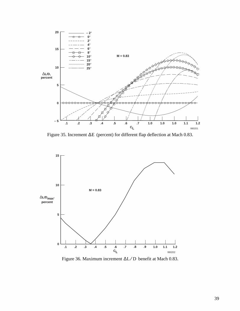
Figure 35. Increment (percent) for different flap deflection at Mach 0.83.

Figure 36. Maximum increment benefit at Mach 0.83.

0

– 5

5

10

15

20

.1 .3.2 .4 .5 .7 1.01.01.0 1.21.1

∆L/D,percent

990201

.6 CL

M = 0.83

– 2°0°2°4°6°8°10°15°20°25°

∆E

0

5

10

15

.1 .3.2 .4 .5 .7 .9.8 1.0 1.21.1

∆L/Dmax,

percent

990202

.6CL

M = 0.83

∆L D⁄

39

Figure 37. Optimal angle of trailing edge.

– 2

4

10

16

2

8

14

0

6

12

.1 .3.2 .4 .5 .7 .9.8 1.0 1.21.1

Angle offlaps orailerons,

deg

990203

.6 CL

M = 0.83

40

REPORT DOCUMENTATION PAGE Form ApprovedOMB No. 0704-0188

Public reporting burden for this collection of information is estimated to average 1 hour per response, including the time for reviewing instructions, searching existing data sources, gathering andmaintaining the data needed, and completing and reviewing the collection of information. Send comments regarding this burden estimate or any other aspect of this collection of information,including suggestions for reducing this burden, to Washington Headquarters Services, Directorate for Information Operations and Reports, 1215 Jefferson Davis Highway, Suite 1204, Arlington,VA 22202-4302, and to the Office of Management and Budget, Paperwork Reduction Project (0704-0188), Washington, DC 20503.

1. AGENCY USE ONLY (Leave blank) 2. REPORT DATE 3. REPORT TYPE AND DATES COVERED

4. TITLE AND SUBTITLE 5. FUNDING NUMBERS

6. AUTHOR(S)

8. PERFORMING ORGANIZATION REPORT NUMBER

7. PERFORMING ORGANIZATION NAME(S) AND ADDRESS(ES)

9. SPONSORING/MONITORING AGENCY NAME(S) AND ADDRESS(ES) 10. SPONSORING/MONITORING AGENCY REPORT NUMBER

11. SUPPLEMENTARY NOTES

12a. DISTRIBUTION/AVAILABILITY STATEMENT 12b. DISTRIBUTION CODE

13. ABSTRACT (Maximum 200 words)

14. SUBJECT TERMS 15. NUMBER OF PAGES

16. PRICE CODE

17. SECURITY CLASSIFICATION OF REPORT

18. SECURITY CLASSIFICATION OF THIS PAGE

19. SECURITY CLASSIFICATION OF ABSTRACT

20. LIMITATION OF ABSTRACT

NSN 7540-01-280-5500 Standard Form 298 (Rev. 2-89)Prescribed by ANSI Std. Z39-18298-102

Estimated Benefits of Variable-Geometry Wing Camber Control forTransport Aircraft.

WU 522 16 14 00 39 00 L10

Alexander Bolonkin and Glenn B. Gilyard

NASA Dryden Flight Research CenterP.O. Box 273Edwards, California 93523-0273

H-2368

National Aeronautics and Space AdministrationWashington, DC 20546-0001 NASA/TM-1999-206586

Analytical benefits of variable-camber capability on subsonic transport aircraft are explored. Usingaerodynamic performance models, including drag as a function of deflection angle for control surfaces ofinterest, optimal performance benefits of variable camber are calculated. Results demonstrate that if all wingtrailing-edge surfaces are available for optimization, drag can be significantly reduced at most points within theflight envelope. The optimization approach developed and illustrated for flight uses variable camber foroptimization of aerodynamic efficiency (maximizing the lift-to-drag ratio). Most transport aircraft havesignificant latent capability in this area. Wing camber control that can affect performance optimization fortransport aircraft includes symmetric use of ailerons and flaps. In this paper, drag characteristics for aileron andflap deflections are computed based on analytical and wind-tunnel data. All calculations based on predictionsfor the subject aircraft and the optimal surface deflection are obtained by simple interpolation for givenconditions. An algorithm is also presented for computation of optimal surface deflection for given conditions.Benefits of variable camber for a transport configuration using a simple trailing-edge control surface systemcan approach more than 10 percent, especially for nonstandard flight conditions. In the cruise regime, thebenefit is 1–3 percent.

Adaptive control, Aircraft performance, Cambered wings, Commercial aircraft,Lift-to-Drag ratio, Optimization, Variable-camber wing.

A03

50

Unclassified Unclassified Unclassified Unlimited

October 1999 Technical Memorandum

Alexander Bolonkin, Senior Research Associate of the National Research Council, Washington D. C. andGlenn B. Gilyard, NASA Dryden Flight Research Center, Edwards, California.

Unclassified—UnlimitedSubject Categories 02-01, 02-03, 03-01