Essentials of Biological Image Analysis

Volker BaeckerINSERM

BioCampus Montpellier (UMS 3426)MRI­TIGR

27/04/2012

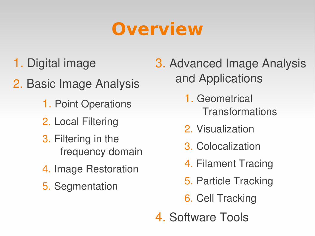
Overview

1. Digital image

2. Basic Image Analysis

1. Point Operations

2. Local Filtering

3. Filtering in the frequency domain

4. Image Restoration

5. Segmentation

3. Advanced Image Analysis and Applications

1. Geometrical Transformations

2. Visualization

3. Colocalization

4. Filament Tracing

5. Particle Tracking

6. Cell Tracking

4. Software Tools

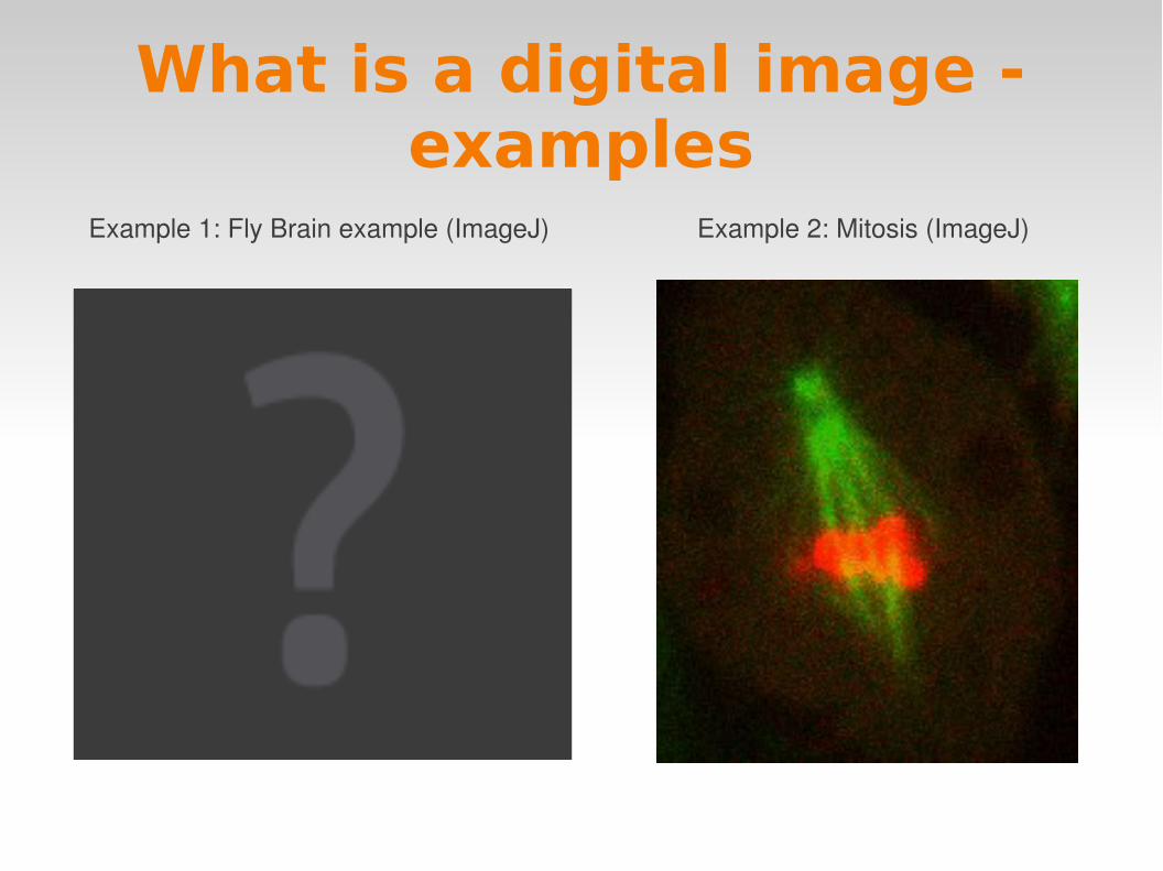
What is a digital image - examples

Example 1: Fly Brain example (ImageJ) Example 2: Mitosis (ImageJ) 

What is a digital image – mathematical point of view Matrix of sample values

finite number of samples

finite number of values per sample

Image dimensions 1D, 2D, 2D + t, 3D, 

3D + t, 3D + t + multispectral

I(x,y,z,t)∈Wn

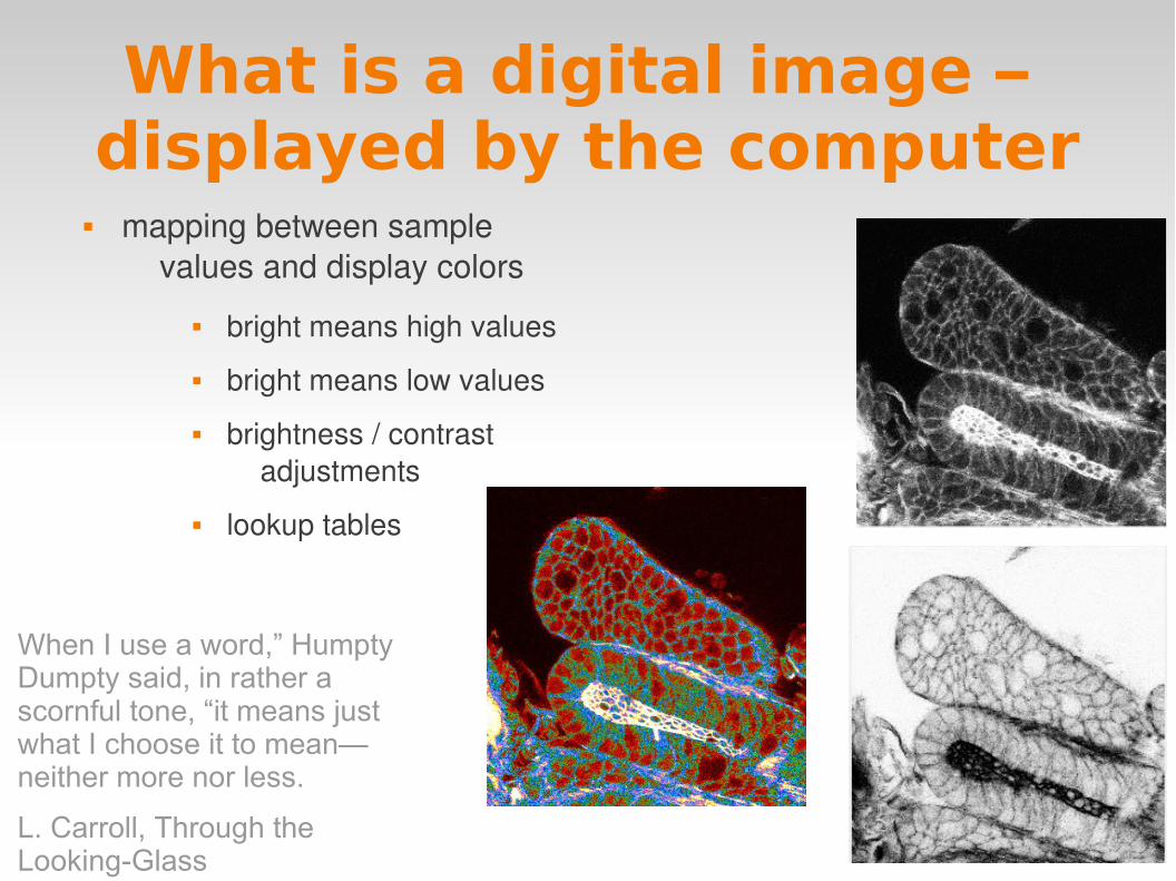
What is a digital image – displayed by the computer

mapping between sample values and display colors

bright means high values

bright means low values

brightness / contrast adjustments

lookup tables

When I use a word,” Humpty Dumpty said, in rather a scornful tone, “it means just what I choose it to mean—neither more nor less.

L. Carroll, Through the Looking-Glass

mapping between sample grid and display grid

homogenous rectangles 

interpolation

What is a digital image – displayed by the computer

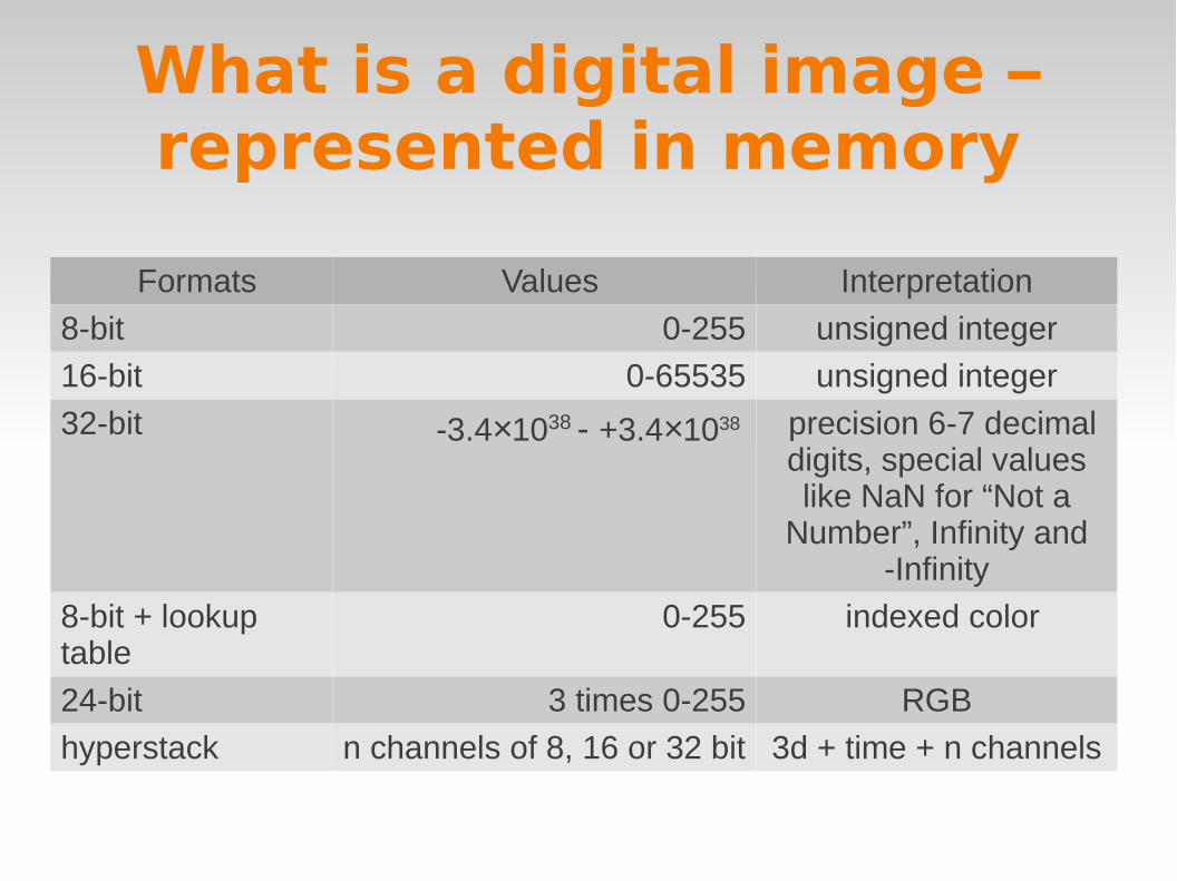
What is a digital image – represented in memory

Formats Values Interpretation

8-bit 0-255 unsigned integer

16-bit 0-65535 unsigned integer

32-bit -3.4×1038 - +3.4×1038 precision 6-7 decimal digits, special values like NaN for “Not a

Number”, Infinity and -Infinity

8-bit + lookup table

0-255 indexed color

24-bit 3 times 0-255 RGB

hyperstack n channels of 8, 16 or 32 bit 3d + time + n channels

What is a digital image – convertion traps

Label Mean Min Max IntDen

green 100.9 0 4095 13774198

10 x green 1009.0 0 40950 137741980

green 8bit 6.3 0 255 861340

10 x 8bit 6.3 0 255 861340

conversion is done by linearly scaling from min–max to 0–255 

look at green channel

multiply by ten

convert both to 8­bit

compare total intensity before and after

What is a digital image – stored on a disk

data (sample values) + meta­data in header

different organization of data and meta­data

different possibilities / restraints format name provider properties

tiff Tagged image file format Adobe lossless / metadata

ome-tiff Open microscopy environment-tiff

OME tiff with ontology for microscopy metadata

jpeg exif Joint Photographic Experts Group - exchangable image file format

ISO lossy data compression / minimal metadata

lsm, stk Laser scanning microscope file

Zeiss extensions of tiff

lif Leica image file format Leica can contain multiple images in one file

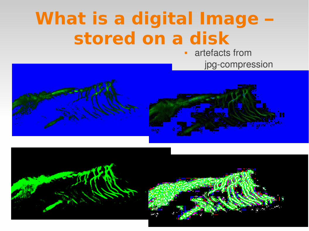
What is a digital Image – stored on a disk

artefacts from jpg­compression

What is a digital image - the image and the real world

sampling and resolution digital image – finite number of samples

Nyquist­Shannon sampling theorem:The sampling interval must be smaller than one­half the size of the smallest resolvable feature of the optical image

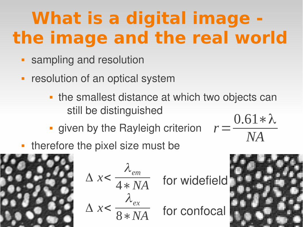
sampling and resolution

resolution of an optical system 

the smallest distance at which two objects can still be distinguished

given by the Rayleigh criterion therefore the pixel size must be

for widefield

for confocal

What is a digital image - the image and the real world

r=0.61∗λ

NA

Δ x<λem

4∗NA

Δ x<λex

8∗NA

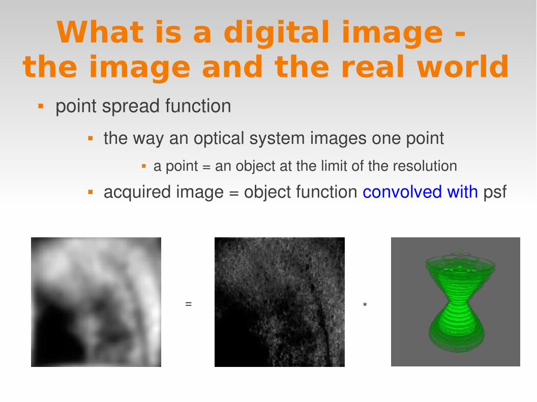
point spread function the way an optical system images one point

a point = an object at the limit of the resolution

acquired image = object function convolved with psf

What is a digital image - the image and the real world

= *

What is a digital image -image and perception

How many colors do you see?

the image contains 3 different colors

the brain interprets color according to the background

What is a digital image -image and perception

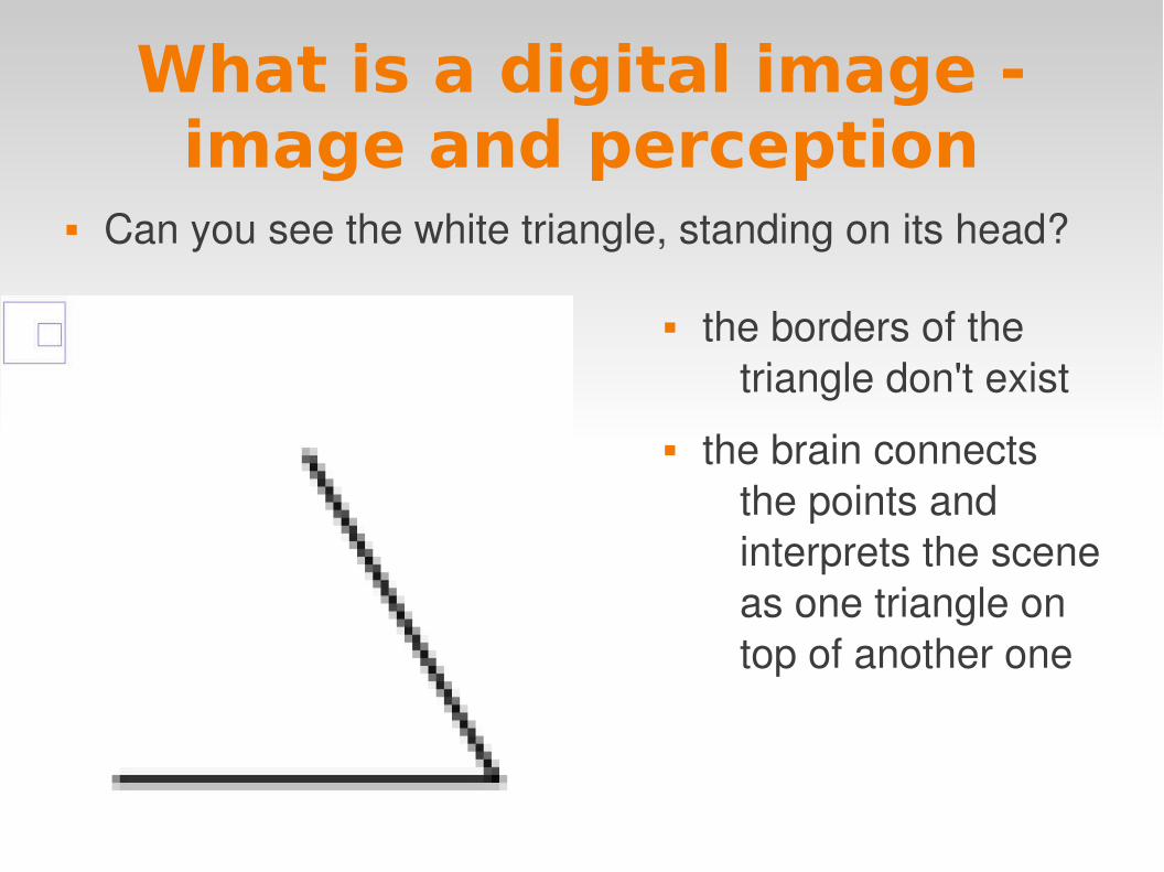
Can you see the white triangle, standing on its head?

the borders of the triangle don't exist

the brain connects the points and interprets the scene as one triangle on top of another one

Wikipedia ”Image analysis is the extraction of meaningful 

information from images; mainly from digital images by means of digital image processing techniques.”

What is image analysis?

IMAGE IN – FEATURES OUT

global intensity transformations intensity inversion contrast and brightness adjustment

linear  gamma function histogram equalization

pseudo­coloring intensity thresholding

Point operations

Point operations – contrast stretching

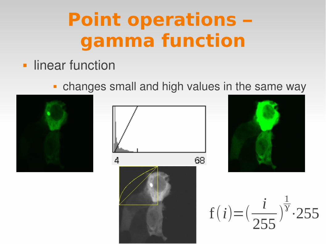
linear function  changes small and high values in the same way

Point operations – gamma function

f ( i)=(i

255)1γ⋅255

Point operations – lookup tables

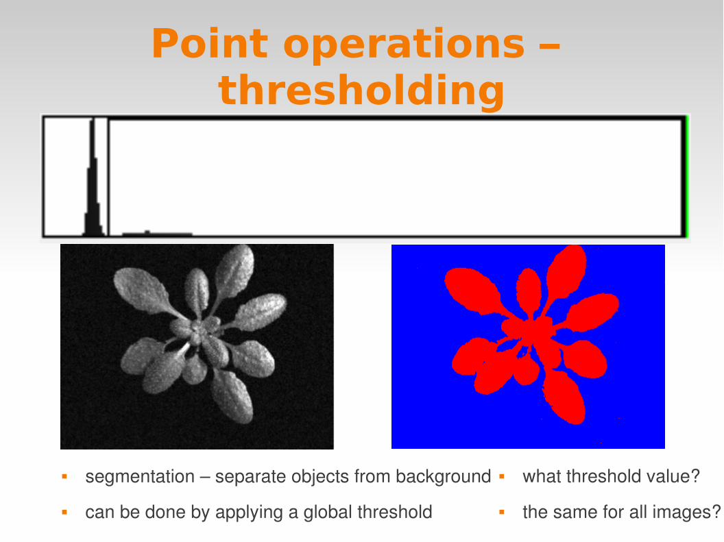
Point operations – thresholding

what threshold value?

the same for all images?

segmentation – separate objects from background

can be done by applying a global threshold

Local Filtering convolution filter (linear filtering)

smoothing mean filter gaussian blur filter

edge detection sobel filter

spot detection Laplacian of Gaussian (Mexican Hat Filter)

ranking filter median, min, max

mathematical morphology

post processing erode, dilate, open, close, top hat, granulometry

The new value of a pixel is calculated from the values in the local neighborhood of the pixel

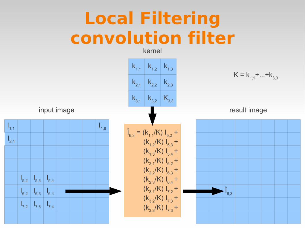
Local Filteringconvolution filter

K = k1,1

+...+k3,3

Î6,3

= (k1,1

/K) I5,2

+(k

1,2/K) I

5,3 +

(k1,3

/K) I5,4

+(k

2,1/K) I

6,2 +

(k2,2

/K) I6,3

+(k

2,3/K) I

6,4 +

(k3,1

/K) I7,2

+(k

3,2/K) I

7,3 +

(k3,3

/K) I7,3

+

I1,1

I1,8

I2,1

I5,2

I5,3

I5,4

I6,2

I6,3

I6,4

I7,2

I7,3

I7,4

input image

Î6,3

result image

k1,1

k1,2

k1,3

k2,1

k2,2

k2,3

k3,1

k3,2

K3,3

kernel

Convolution filter - smoothing

1 1 1

1 1 1

1 1 1

mean

Convolution filter - smoothing gaussian blur

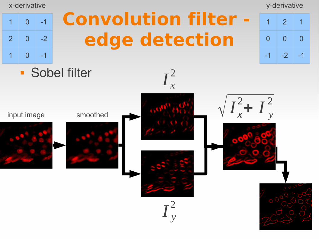
Sobel filter

√ I x2+ I y

2

I x2

I y2

smoothed

Convolution filter - edge detection

input image

1 0 -1

2 0 -2

1 0 -1

x-derivative

1 2 1

0 0 0

-1 -2 -1

y-derivative

LoG

Laplacian filter enhaces spots but augments noise

Convolution filter - spot detection

use 'Laplacian of Gaussian (LoG)' to enhance spots in noisy images  

-1 -1 -1

-1 8 -1

-1 -1 -1

laplacian

Local Filtering -Ranking filter

for each pixel:  sort the values in the neighborhood take the value at a given position

first = min filter enlarge dark regions middle = median filter filter noise last = max filter enlarge bright regions

12, 13, 14, 15, 18, 19, 21, 27, 29

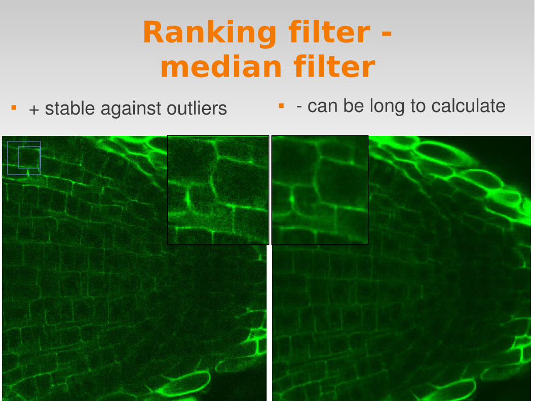
Ranking filter -median filter

+ stable against outliers  ­ can be long to calculate

correct segmentation, measure features, granulometry, edge detection, skeletonization, reconstruct objects

work on a mask (a binary image)

move the structuring element along the image

two basic operations dilate (enlarge objects): 

current pixel is 1 if the SE touches a 1 in the image

erode (shrink objects): current pixel is 1 if no 1 in the SE touches a zero in the 

image  

Local Filteringbinary morphology

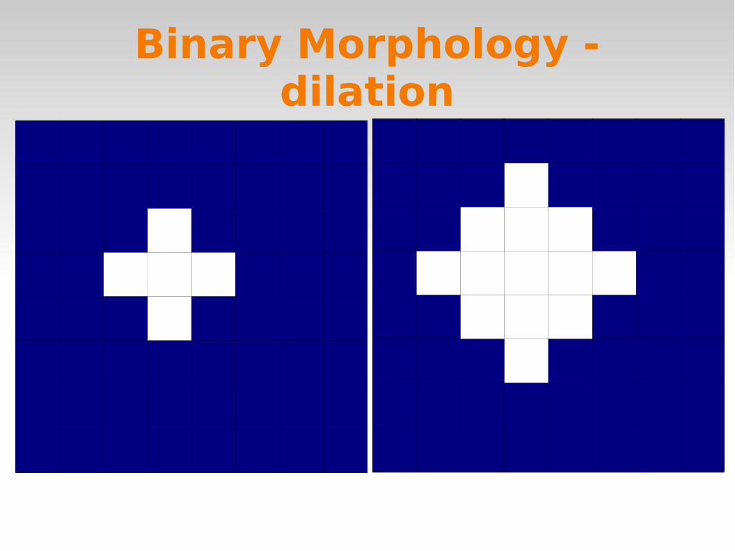
Binary Morphology -dilation

Binary Morphology -erosion

close(X) = dilate(erode(X)) close holes in objects

open(X) = erode(dilate(X)) remove small objects

Binary Morphology -open and close

in dilate erode

close open

Binary Morphology -applications

I

dilate(I) - erode(I)

edge detection skeletonization granulometry

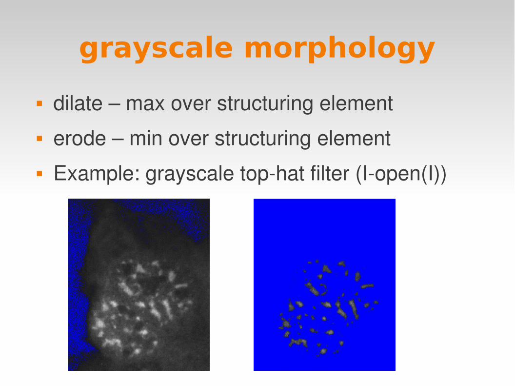
grayscale morphology

dilate – max over structuring element erode – min over structuring element Example: grayscale top­hat filter (I­open(I)) 

filtering in the frequency domain

Fourier Transform  low­pass high­pass band­pass correlation convolution

filtering in the frequency domain – fourier transform

F (ν)=∫ f ( x)e−i2π ν xdx

signal can be represented as sum of sinoids

FT transforms from spatial to frequency domain

Filtering in the frequency domain

FFT

select frequencies

Inverse FFT

Filtering in the frequency domain

Low pass filter

High pass filter

Filtering in the frequency domain

Band pass filter

Image Restoration

Image degraded Noise

quantum nature of light (poisson distribution) imperfect electronics (gaussian distribution)

Background imperfect illumination

Blur out of focus light

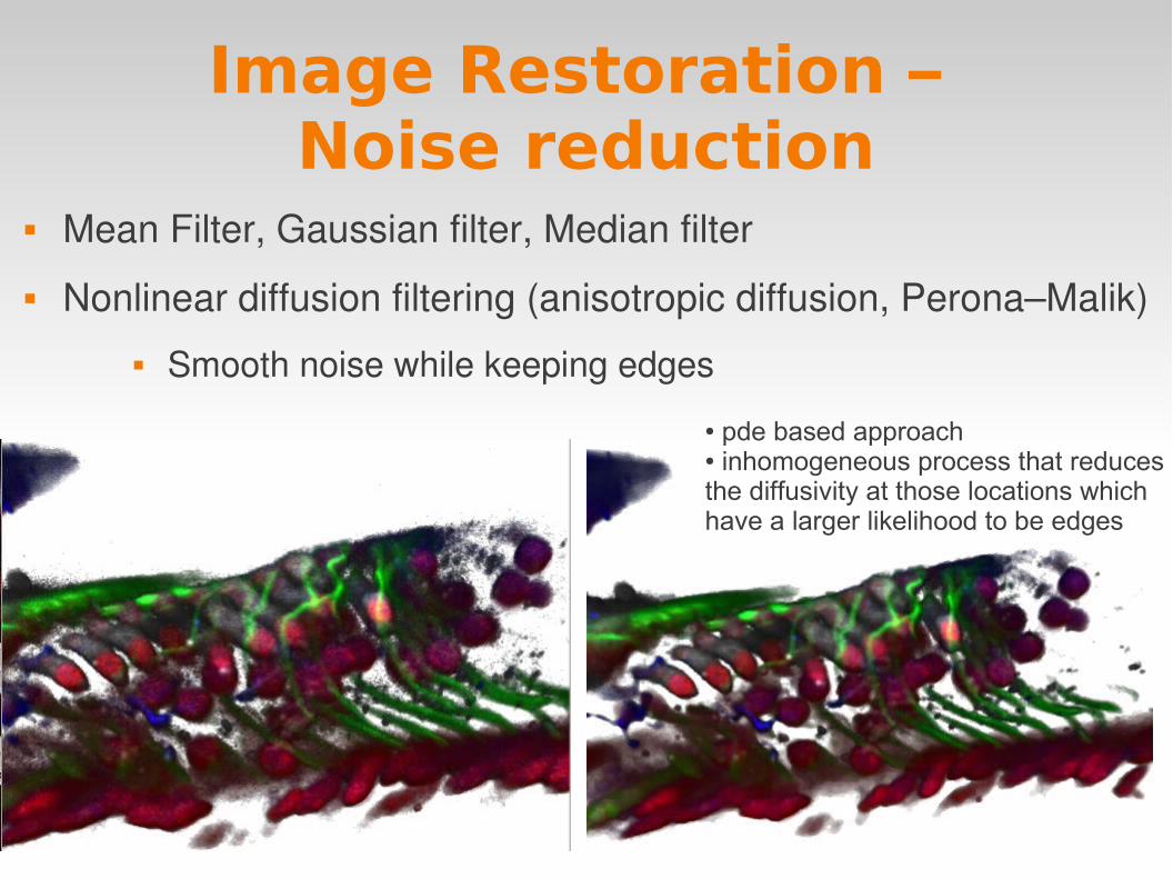
Mean Filter, Gaussian filter, Median filter

Nonlinear diffusion filtering (anisotropic diffusion, Perona–Malik) Smooth noise while keeping edges

Image Restoration – Noise reduction

● pde based approach● inhomogeneous process that reduces the diffusivity at those locations which have a larger likelihood to be edges

correct inhomogenous illumination correct with image of background if not available: estimate background image

Image Restoration -Background subtraction

IB⋅mean(B)

blur diffraction out­of­focus light

acquired image = object function convolved with psf

Image Restoration - Deconvolution

= *

Deconvolution -examples

Segmentation

separate objects from background and objects from each other

region growing clustering watershed transform

Segmentation - region growing

● start from seed­points● simultaneously grow regions

● stop according to a homogenity criterium

Segmentation -Watershed

interpret intensity as valleys fill slowly with rising water whenever two basins join create a separation

Segmentation -Watershed

problem: over­segmentation

possible solution: seeded watershed number of final basins = number of seeds

Geomectrical Transformation

problem: image is spatially distorted or

mismatch between channels due to chromatic aberration barrel distortion or pincushion distortion speciman moved during acquisition

lacks spatial correspondence histological slices combining images from different sources stitching of images of a mosaic

solution: image registration or alignment

Image Registration

Image registration coordinate transformation

landmark based manually selected automtically extracted 

intensity based calculate match between images

possible transformations rigid, affine, curved

resampling interpolation

nearest neighbor, linear, cubic spline 

Example Registration

spinal cordgrey mattertraumatic lesion

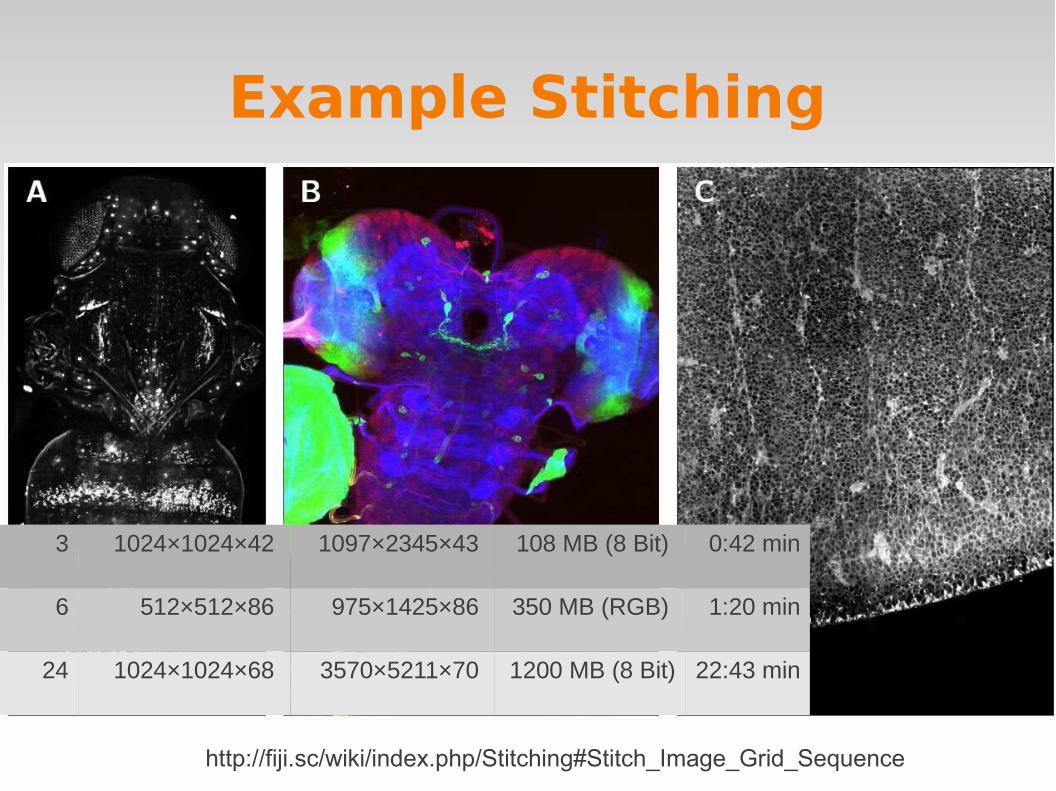
Example Stitching

http://fiji.sc/wiki/index.php/Stitching#Stitch_Image_Grid_Sequence

3 1024×1024×42 1097×2345×43 108 MB (8 Bit) 0:42 min

6 512×512×86 975×1425×86 350 MB (RGB) 1:20 min

24 1024×1024×68 3570×5211×70 1200 MB (8 Bit) 22:43 min

Visualization

how to understand multidimensional data? reduce dimensionality in a sensible way

methods volume rendering

methods that use the raw data directly without geometrical representation

ray tracing maximum intensity projection (MIP) blend (calculated from all information along the ray)

surface rendering take into account only surfaces of objects needs a description of the object in terms of 

geometrical entities

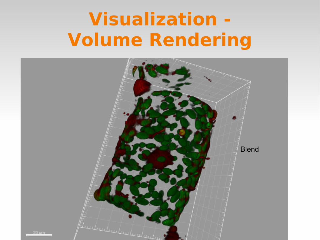
Visualization -Volume Rendering

how does the volume interact with a ray of light given position and parameters of the light source given the position of the observer

MIP Blend

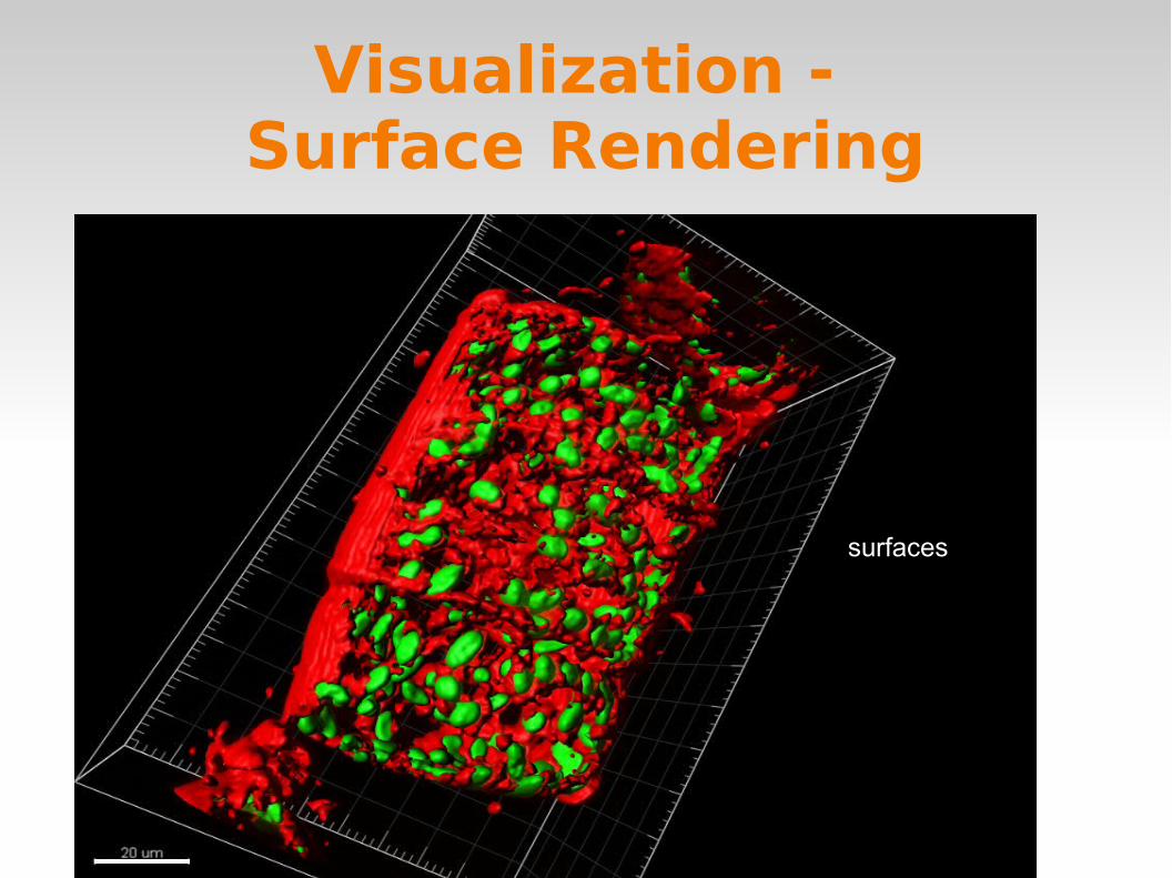
Visualization - Surface Rendering

segmentation of the object surface triangulation 

marching cubes algorithm

surfaces

Visualization - Mixed Rendering

Mixed renderingretina

mixed rendering with transparence

Colocalization Analysis

Wikipedia:

”colocalization refers to observation of the spatial overlap between two (or more) different fluorescent labels, each having a separate emission wavelength, to see if the different "targets" are located in the same area of the cell or very near to one another. ”

”correlation, ... indicative of a biological interaction”

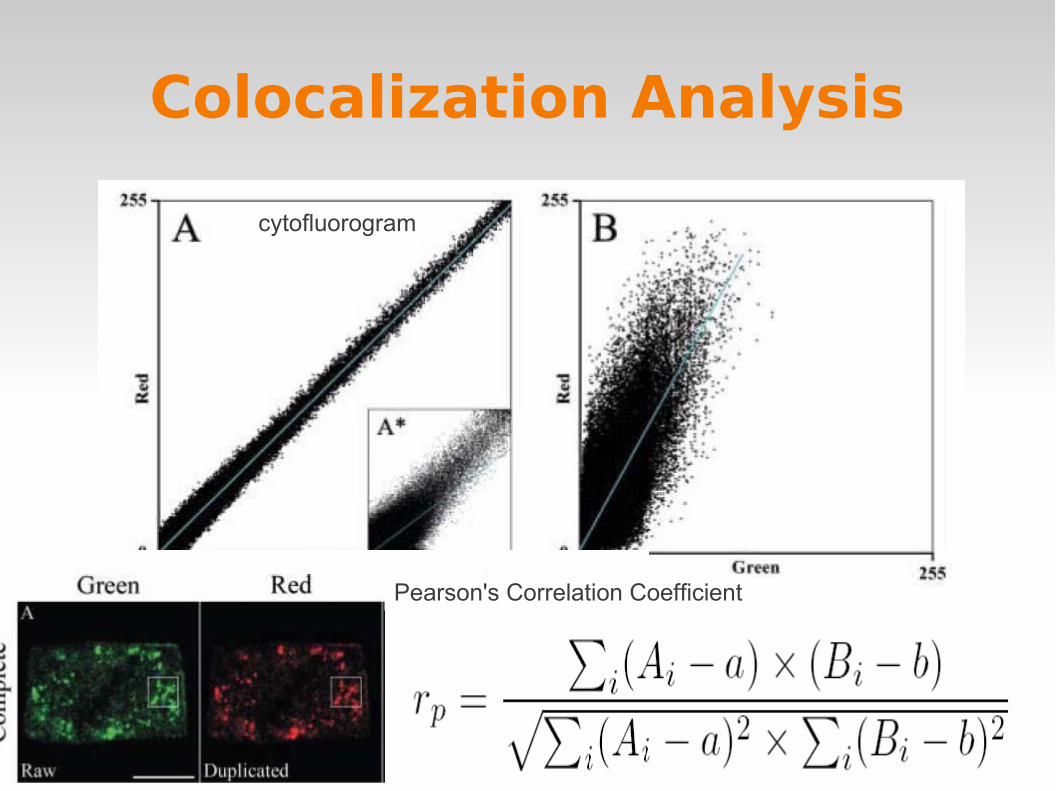
Colocalization Analysis

cytofluorogram

Pearson's Correlation Coefficient

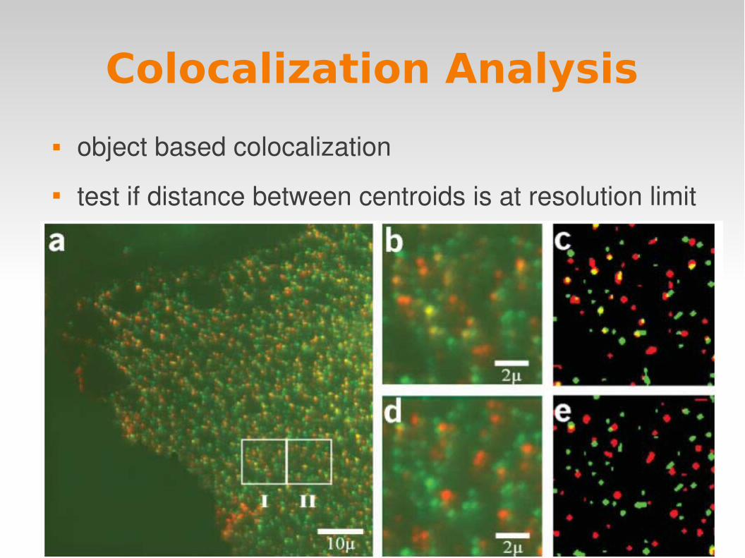
Colocalization Analysis

object based colocalization

test if distance between centroids is at resolution limit 

Filament tracing and analysis

possible approach second order derivatives (hessian matrix) cost image shortest paths

automatic or semi­interacitve  spine detection

Filament tracing and analysis

Particle detection and tracking

2 steps detection of particles (spots) per time­frame

least­squares fitting of a gaussian mixture model to the image data

linking of particles in successive frames problem: number not constant over time

Particle detection and tracking

Cell segmentation and tracking

cells have a distinct shape shape may change over time use active contours (snakes) to detect cells

active surfaces in 3D shape constraint fitting to image data

tracking use contour of cell at t=n 

as initial contour for cell at t=n+1

Cell segmentation and tracking

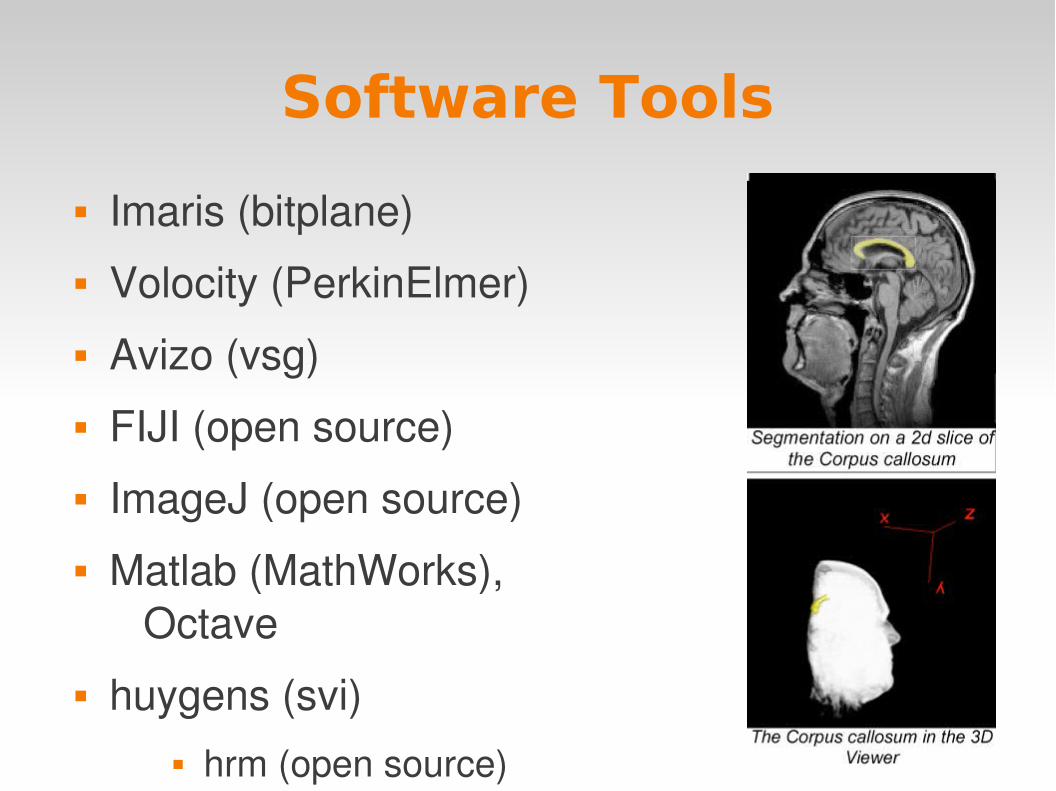
Software Tools

Imaris (bitplane) Volocity (PerkinElmer) Avizo (vsg) FIJI (open source) ImageJ (open source) Matlab (MathWorks), 

Octave huygens (svi) 

hrm (open source)

Thank you

Questions?