Essential University Physics Volume 2 - Pearson

383

OVERVIEW

Electromagnetism is one of the fundamental forces, and it governs the behavior of matter from the atomic scale to the macroscopic world.

Electromagnetic technology, from computer micro-chips to cell phones and on to large electric motors and generators, is essential to modern society. Even our bodies rely heavily on electromagnetism: Electric signals pace our heartbeat, electrochemical process-es transmit nerve impulses, and the electric structure of cell membranes mediates the flow of materials into and out of the cell.

Four fundamental laws describe electricity and magnetism. Two deal separately with the two

phenomena, while the others reveal profound connections that make electricity and magne-tism aspects of a single phenomenon that we call electromagnetism. In this part you’ll come to understand those fundamental laws, learn how electromagnetism determines the structure and behavior of nearly all matter, and explore the electromagnetic technologies that play so important a role in your life. Finally, you’ll see how the laws of electromagnetism lead to electromagnetic waves and thus help us understand the nature of light.

Electricity constitutes a significant portion of humankind’s energy, as evidenced by this composite satellite image of Earth at night. Nearly all that electrical energy is produced by generators, devices that exploit an intimate relation between electricity and magnetism.

ElectromagnetismPART FOUR

M20_WOLF1186_04_GE_C20.indd 383 19/05/20 1:02 AM

Sample

page

s

384

What holds your body together? What keeps a skyscraper standing? What holds your car on the road as you round a turn? What gov-

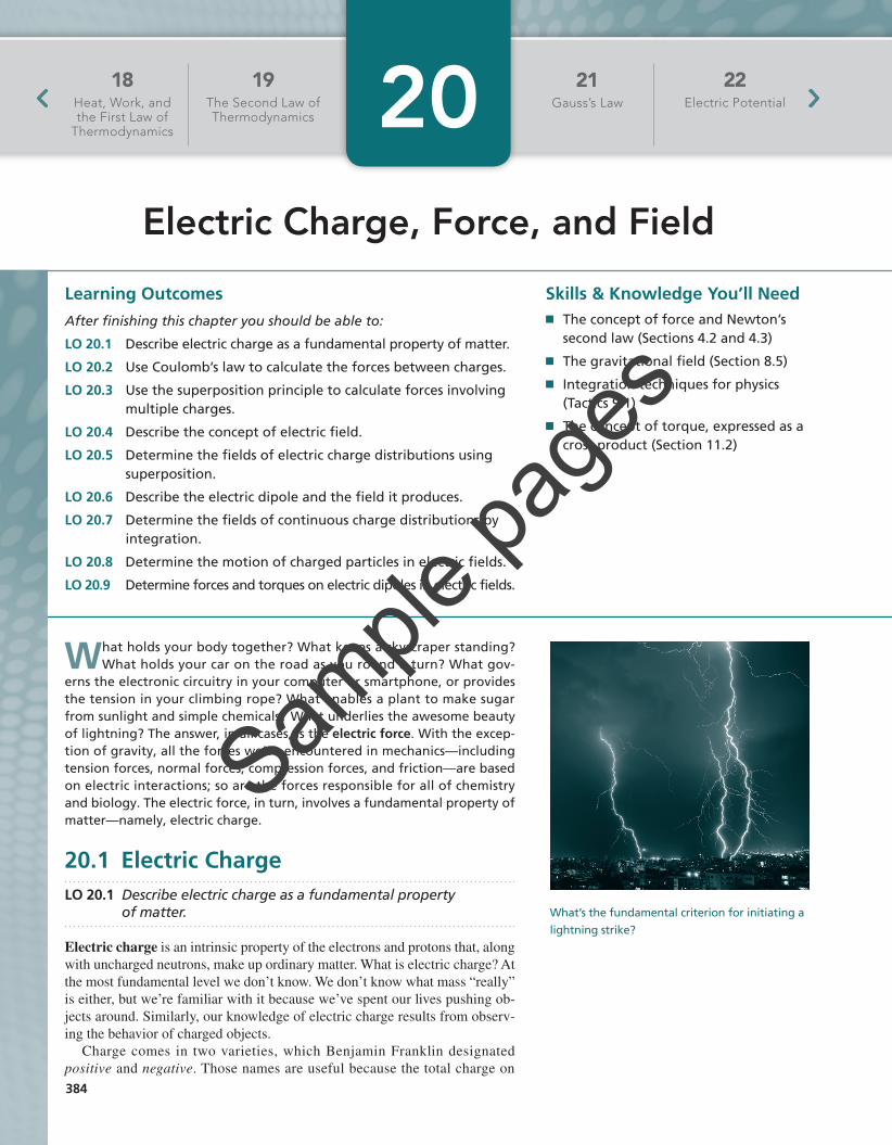
erns the electronic circuitry in your computer or smartphone, or provides the tension in your climbing rope? What enables a plant to make sugar from sunlight and simple chemicals? What underlies the awesome beauty of lightning? The answer, in all cases, is the electric force. With the excep-tion of gravity, all the forces we’ve encountered in mechanics—including tension forces, normal forces, compression forces, and friction—are based on electric interactions; so are the forces responsible for all of chemistry and biology. The electric force, in turn, involves a fundamental property of matter—namely, electric charge.

20.1 Electric ChargeLO 20.1 Describe electric charge as a fundamental property

of matter.

Electric charge is an intrinsic property of the electrons and protons that, along with uncharged neutrons, make up ordinary matter. What is electric charge? At the most fundamental level we don’t know. We don’t know what mass “really” is either, but we’re familiar with it because we’ve spent our lives pushing ob-jects around. Similarly, our knowledge of electric charge results from observ-ing the behavior of charged objects.

Charge comes in two varieties, which Benjamin Franklin designated positive and negative. Those names are useful because the total charge on

Learning OutcomesAfter finishing this chapter you should be able to:

LO 20.1 Describe electric charge as a fundamental property of matter.

LO 20.2 Use Coulomb’s law to calculate the forces between charges.

LO 20.3 Use the superposition principle to calculate forces involving multiple charges.

LO 20.4 Describe the concept of electric field.

LO 20.5 Determine the fields of electric charge distributions using superposition.

LO 20.6 Describe the electric dipole and the field it produces.

LO 20.7 Determine the fields of continuous charge distributions by integration.

LO 20.8 Determine the motion of charged particles in electric fields.

LO 20.9 Determine forces and torques on electric dipoles in electric fields.

Electric Charge, Force, and Field

22Electric Potential20 21

Gauss’s Law

19The Second Law of Thermodynamics

18Heat, Work, and the First Law of

Thermodynamics

What’s the fundamental criterion for initiating a lightning strike?

Skills & Knowledge You’ll Need■■ The concept of force and Newton’s

second law (Sections 4.2 and 4.3)

■■ The gravitational field (Section 8.5)

■■ Integration techniques for physics (Tactics 9.1)

■■ The concept of torque, expressed as a cross product (Section 11.2)

M20_WOLF1186_04_GE_C20.indd 384 19/05/20 1:02 AM

Sample

page

s

20.2 Coulomb’s Law 385

an object—the object’s net charge—is the algebraic sum of its constituent charges. Like charges repel, and opposites attract, a fact that constitutes a qualitative description of the electric force.

Quantities of ChargeAll electrons carry the same charge, and all protons carry the same charge. The proton’s charge has exactly the same magnitude as the electron’s, but with opposite sign. Given that electrons and protons differ substantially in other properties—like mass—this elec-tric relation is remarkable. Exercise 11 shows how dramatically different our world would be if there were even a slight difference between the magnitudes of the electron and proton charges.

The magnitude of the electron or proton charge is the elementary charge e. Electric charge is quantized; that is, it comes only in discrete amounts. In a famous experiment in 1909, the American physicist R. A. Millikan measured the charge on small oil drops and found it was always a multiple of a basic value we now know as the elementary charge.

Elementary particle theories show that the fundamental charge is actually 13 e. Such

“fractional charges” reside on quarks, the building blocks of protons, neutrons, and many other particles. Quarks always join to produce particles with integer multiples of the full elementary charge, and it seems impossible to isolate individual quarks.

The SI unit of charge is the coulomb (C), named for the French physicist Charles Augustin de Coulomb (1736–1806). From the late 19th century to the early 21st cen-tury, the coulomb was defined in terms of electric current and time—a definition that was difficult to implement in practice. The 2019 revision of the SI gave the cou-lomb a much simpler definition. Now, the elementary charge is defined to be exactly 1.602176634 * 10-19 C. The coulomb is therefore the number of elementary charges equal to the inverse of this number. For our purposes, that’s about 6.24 * 1018 elemen-tary charges.

Charge ConservationElectric charge is a conserved quantity, meaning that the net charge in a closed region remains constant. Charged particles may be created or annihilated, but always in pairs of equal and opposite charge. The net charge always remains the same.

FS

FS

FIGURE 20.1 Two balloons carrying similar electric charges repel each other.

20.2 Coulomb’s LawLO 20.2 Use Coulomb’s law to calculate the forces between charges.

LO 20.3 Use the superposition principle to calculate forces involving multiple charges.

Rub a balloon; it gets charged and sticks to your clothing. Charge another balloon, and the two repel (Fig. 20.1). Socks cling to your clothes as they come from the dryer, and bits of Styrofoam cling annoyingly to your hands. Walk across a carpet, and you’ll feel a shock when you touch a doorknob. All these are common examples where you’re directly aware of electric charge.

Electricity would be unimportant if the only significant electric interactions were these obvious ones. In fact, the electric force dominates all interactions of everyday matter, from the motion of a car to the movement of a muscle. It’s just that matter on a large scale

20.1 The proton is a composite particle composed of three quarks, all of which are either up quarks (u; charge +2

3 e) or down quarks (d; charge -13 e). (More on quarks

in Chapter 39.) Which of these quark combinations is the proton? (a) udd; (b) uuu; (c) uud; (d) dddG

OT

IT?

M20_WOLF1186_04_GE_C20.indd 385 19/05/20 1:02 AM

Sample

page

s

386 Chapter 20 Electric Charge, Force, and Field

is almost perfectly neutral, meaning it carries zero net charge. Therefore, electric effects aren’t obvious. But at the molecular level, the electric nature of matter is immediately evident (Fig. 20.2).

Attraction and repulsion of electric charges imply a force. Joseph Priestley and Charles Augustin de Coulomb investigated this force in the late 1700s. They found that the force between two charges acts along the line joining them, with the magnitude proportional to the product of the charges and inversely proportional to the square of the distance between them. Coulomb’s law summarizes these results:

rn

rn

rnkq1q2

r2F12 =

F12

The unit vector ralways points away from q1.

(a)

(b)

r

q1 q2

F12

r

q1 q2

n

n

n

Here the productq1q2 is positive,so F12 is in thesame directionas r.

S

Here the charges have opposite signs, so q1q2 6 0 and F12 points opposite r.

S

S

S

S

FIGURE 20.3 Quantities in Coulomb’s law for calculating the force F

S12 that q1 exerts

on q2.

FS

12 =kq1q2

r2 rn 1Coulomb>s law2 (20.1)

FS

12 is the force charge q1 exerts on charge q2.

k is approximately 9.0 * 109 N #m2/C2. q1 and q2 are two charges.

r is the distance between the two charges.

rn is a unit vector that points from q1 toward q2 regardless of the signs of the charges.

where FS

12 is the force charge q1 exerts on q2 and r is the distance between the charges. In SI the proportionality constant k has the approximate value 9.0 * 109 N # m2/C2. Force is a vector, and rn is a unit vector that helps determine its direction. Figure 20.3 shows that rn lies on a line passing through the two charges and points in the direction from q1 toward q2. Reverse the roles of q1 and q2, and you’ll see that F

S21 has the same

magnitude as FS

12 but the opposite direction; thus Coulomb’s law obeys Newton’s third law. Figure 20.3 also shows that the force is in the same direction as the unit vector when the charges have the same sign, but opposite the unit vector when the charges have different signs. Thus Coulomb’s law accounts for the fact that like charges repel and opposites attract.

The key to using Coulomb’s law is to remember that force is a vector, and to realize that Coulomb’s law in the form of Equation 20.1 gives both the magnitude and direction of the electric force. Dealing carefully with vector directions is especially important in situations with more than two charges.

INTERPRET First, make sure you’re dealing with the electric force alone. Identify the charge or charges on which you want to calculate the force. Next, identify the charge or charges pro-ducing the force. These comprise the source charge.

DEVELOP Begin with a drawing that shows the charges, as in Fig. 20.4. If you’re given charge coordinates, place the charges on the coordinate system; if not, choose a suitable coordinate system. For each source charge, determine the unit vector(s) in Equation 20.1. If the charges lie along or parallel to a coordinate axis, then the unit vector will be one of the unit vectors in, jn, or kn, perhaps with a minus sign. In Fig. 20.4, the force on q3 due to q1 is such a case. When the two charges don’t lie on a coordinate axis, like q1 and q2 in Fig. 20.4, you can find the unit vec-tor by noting that the displacement vector r

!12 points in the desired direction, from the source

charge to the charge experiencing the force. Dividing r!12 by its own magnitude then gives the

unit vector in the direction of r!12; that is, rn = r

!12/r12.

EVALUATE For each source charge, determine the electric force using Equation 20.1,

FS

12 =1kq1q2/r22rn

with rn the unit vector you’ve just found.

PROBLEM-SOLVING STRATEGY 20.1 Coulomb’s Law

A salt grain iselectrically neutral c

cbut the electricforce is responsiblefor its cubical shape.

(a)

(b)

Na Cl

-

+ +-

+

+

+

++

+

+

-

--

-

-

-

-

+

FIGURE 20.2 (a) A single salt grain is electrically neutral, so the electric force isn’t obvious. (b) Actually, the electric force determines the structure of salt.

M20_WOLF1186_04_GE_C20.indd 386 19/05/20 1:02 AM

Sample

page

s

20.2 Coulomb’s Law 387

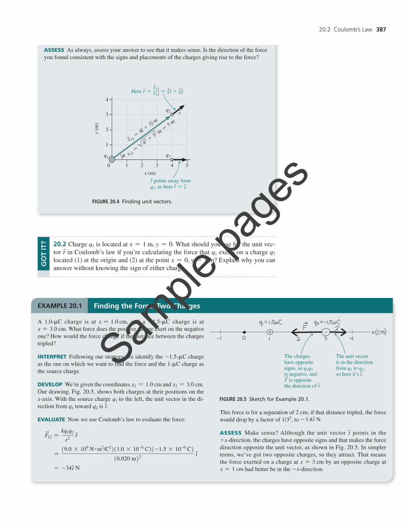
ASSESS As always, assess your answer to see that it makes sense. Is the direction of the force you found consistent with the signs and placements of the charges giving rise to the force?

rn

45

35

r points away fromq1, so here r = i.

i + Here r = =

u

0 1

1

2

3

4

2 3 4 5

q1

x (m)

y (m

)

q2

q3

j.

242 + 3

2 m = 5 m

r 12 =

r12r12

u

n nn

n

r 12 = 4i + 3j

m

u

n

n

n n

FIGURE 20.4 Finding unit vectors.

20.2 Charge q1 is located at x = 1 m, y = 0. What should you use for the unit vec-tor rn in Coulomb’s law if you’re calculating the force that q1 exerts on a charge q2 located (1) at the origin and (2) at the point x = 0, y = 1 m? Explain why you can answer without knowing the sign of either charge.G

OT

IT?

A 1.0@mC charge is at x = 1.0 cm, and a -1.5@mC charge is at x = 3.0 cm. What force does the positive charge exert on the negative one? How would the force change if the distance between the charges tripled?

INTERPRET Following our strategy, we identify the -1.5@mC charge as the one on which we want to find the force and the 1@mC charge as the source charge.

DEVELOP We’re given the coordinates x1 = 1.0 cm and x2 = 3.0 cm. Our drawing, Fig. 20.5, shows both charges at their positions on the x-axis. With the source charge q1 to the left, the unit vector in the di-rection from q1 toward q2 is in.

EVALUATE Now we use Coulomb’s law to evaluate the force:

FS

12 =kq1q2

r2 rn

=19.0 * 109 N # m2/C2211.0 * 10-6 C21-1.5 * 10-6 C2

10.020 m22 in

= -34in N

This force is for a separation of 2 cm; if that distance tripled, the force would drop by a factor of 1/32, to -3.8in N.

ASSESS Make sense? Although the unit vector in points in the +x-direction, the charges have opposite signs and that makes the force direction opposite the unit vector, as shown in Fig. 20.5. In simpler terms, we’ve got two opposite charges, so they attract. That means the force exerted on a charge at x = 3 cm by an opposite charge at x = 1 cm had better be in the -x-direction.

Finding the Force: Two ChargesEXAMPLE 20.1

The chargeshave oppositesigns, so q1q2is negative, and F is oppositethe direction of r.

The unit vectoris in the directionfrom q1 to q2,so here it’s i.

n

Sn

FIGURE 20.5 Sketch for Example 20.1.

M20_WOLF1186_04_GE_C20.indd 387 19/05/20 1:02 AM

Sample

page

s

Point Charges and the Superposition PrincipleCoulomb’s law is strictly true only for point charges—charged objects of negligible size. Electrons and protons can usually be treated as point charges; so, approximately, can any two charged objects if their separation is large compared with their size. But often we’re interested in the electric effects of charge distributions—arrangements of charge spread over space. Charge distributions are present in molecules, memory cells in your computer, your heart, and thunderclouds. We need to combine the effects of two or more charges to find the electric effects of such charge distributions.

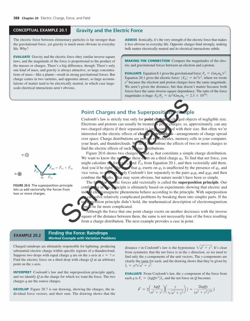
Figure 20.6 shows two charges q1 and q2 that constitute a simple charge distribution. We want to know the net force these exert on a third charge q3. To find that net force, you might calculate the forces F

S13 and F

S23 from Equation 20.1, and then vectorially add them.

And you’d be right: The force that q1 exerts on q3 is unaffected by the presence of q2, and vice versa, so you can apply Coulomb’s law separately to the pairs q1q3 and q2q3 and then combine the results. That may seem obvious, but nature needn’t have been so simple.

The fact that electric forces add vectorially is called the superposition principle. Our confidence in this principle is ultimately based on experiments showing that electric and indeed electromagnetic phenomena behave according to the principle. With superposition we can solve relatively complicated problems by breaking them into simpler parts. If the superposition principle didn’t hold, the mathematical description of electromagnetism would be far more complicated.

Although the force that one point charge exerts on another decreases with the inverse square of the distance between them, the same is not necessarily true of the force resulting from a charge distribution. The next example provides a case in point.

CONCEPTUAL EXAMPLE 20.1 Gravity and the Electric Force

The electric force between elementary particles is far stronger than the gravitational force, yet gravity is much more obvious in everyday life. Why?

EVALUATE Gravity and the electric force obey similar inverse-square laws, and the magnitude of the force is proportional to the product of the masses or charges. There’s a big difference, though: There’s only one kind of mass, and gravity is always attractive, so large concentra-tions of mass—like a planet—result in strong gravitational forces. But charge comes in two varieties, and opposites attract, so large accumu-lations of matter tend to be electrically neutral, in which case large-scale electrical interactions aren’t obvious.

ASSESS Ironically, it’s the very strength of the electric force that makes it less obvious in everyday life. Opposite charges bind strongly, making bulk matter electrically neutral and its electrical interactions subtle.

MAKING THE CONNECTION Compare the magnitudes of the elec-tric and gravitational forces between an electron and a proton.

EVALUATE Equation 8.1 gives the gravitational force: Fg = Gme

mp /r2.

Equation 20.1 gives the electric force: �FE � = ke2/r2, where we wrote e2 because the electron and proton charges have the same magnitude. We aren’t given the distance, but that doesn’t matter because both forces have the same inverse-square dependence. The ratio of the force magnitudes is huge: FE /Fg = ke2/Gme

mp = 2.3 * 1039!

F23

F13

Fnet = F13 + F23

q2

q1

q3

SSS

S

S

FIGURE 20.6 The superposition principle lets us add vectorially the forces from two or more charges.

Charged raindrops are ultimately responsible for lightning, producing substantial electric charge within specific regions of a thundercloud. Suppose two drops with equal charge q are on the x-axis at x = {a. Find the electric force on a third drop with charge Q at an arbitrary point on the y-axis.

INTERPRET Coulomb’s law and the superposition principle apply, and we identify Q as the charge for which we want the force. The two charges q are the source charges.

DEVELOP Figure 20.7 is our drawing, showing the charges, the in-dividual force vectors, and their sum. The drawing shows that the

distance r in Coulomb’s law is the hypotenuse 2a2 + y2. It’s clear from symmetry that the net force is in the y-direction, so we need to find only the y-components of the unit vectors. The y-components are clearly the same for each, and the drawing shows that they’re given by rny = y/2a2 + y2.

EVALUATE From Coulomb’s law, the y-component of the force from each q is Fy = 1kqQ/r22rny, and the net force on Q becomes

FS

= 2 a kqQ

a2 + y2 bay

2a2 + y2b jn =

2kqQy

1a2 + y223/2 jn

Finding the Force: RaindropsWorked Example with Variation Problems

EXAMPLE 20.2


M20_WOLF1186_04_GE_C20.indd 388 19/05/20 1:02 AM

Sample

page

s

20.3 The Electric Field 389

20.3 The Electric FieldLO 20.4 Describe the concept of electric field.

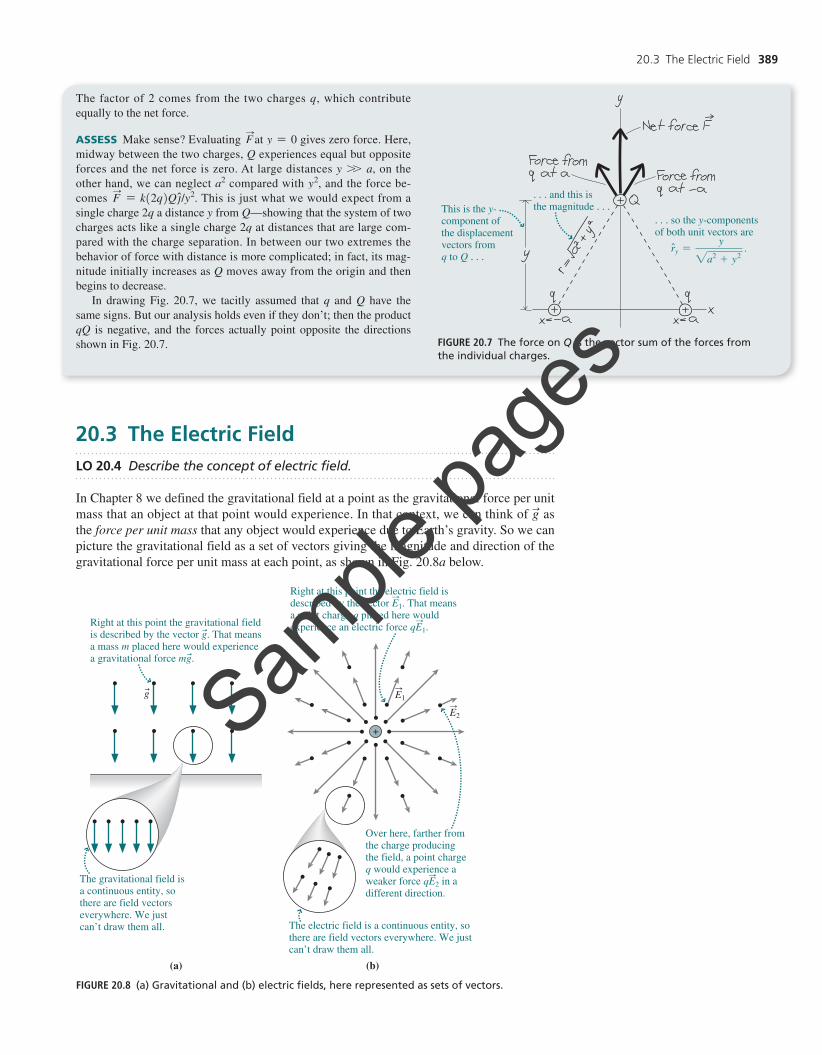
In Chapter 8 we defined the gravitational field at a point as the gravitational force per unit mass that an object at that point would experience. In that context, we can think of g

! as

the force per unit mass that any object would experience due to Earth’s gravity. So we can picture the gravitational field as a set of vectors giving the magnitude and direction of the gravitational force per unit mass at each point, as shown in Fig. 20.8a below.

y

2a2 + y2

This is the y-component ofthe displacementvectors fromq to Q c

cand this isthe magnitude c

cso the y-componentsof both unit vectors are

ry = .n

FIGURE 20.7 The force on Q is the vector sum of the forces from the individual charges.

The factor of 2 comes from the two charges q, which contribute equally to the net force.

ASSESS Make sense? Evaluating FS

at y = 0 gives zero force. Here, midway between the two charges, Q experiences equal but opposite forces and the net force is zero. At large distances y W a, on the other hand, we can neglect a2 compared with y2, and the force be-comes F

S= k12q2Qjn/y2. This is just what we would expect from a

single charge 2q a distance y from Q—showing that the system of two charges acts like a single charge 2q at distances that are large com-pared with the charge separation. In between our two extremes the behavior of force with distance is more complicated; in fact, its mag-nitude initially increases as Q moves away from the origin and then begins to decrease.

In drawing Fig. 20.7, we tacitly assumed that q and Q have the same signs. But our analysis holds even if they don’t; then the product qQ is negative, and the forces actually point opposite the directions shown in Fig. 20.7.

E2S

E1S

(a) (b)

The gravitational field is a continuous entity, so there are field vectors everywhere. We just can’t draw them all.

Right at this point the gravitational field is described by the vector g. That means a mass m placed here would experience a gravitational force mg.

Over here, farther from the charge producing the field, a point charge q would experience a weaker force qE2 in a different direction.

The electric field is a continuous entity, so there are field vectors everywhere. We just can’t draw them all.

gu

u

u

S

S

SRight at this point the electric field is described by the vector E1. That means a point charge q placed here would experience an electric force qE1.

FIGURE 20.8 (a) Gravitational and (b) electric fields, here represented as sets of vectors.

M20_WOLF1186_04_GE_C20.indd 389 19/05/20 1:02 AM

Sample

page

s


The electric field exists at every point in space. When we represent the field by vec-tors, we can’t draw one everywhere, but that doesn’t mean there isn’t a field at all points. Furthermore, we draw vectors as extended arrows, but each vector represents the field at only one point—namely, the tail end of the vector. Figure 20.8b illustrates this for the electric field of a point charge.

The field concept leads to a shift in our thinking about forces. Instead of the action-at-a-distance idea that Earth reaches across empty space to pull on the Moon, the field concept says that Earth creates a gravitational field and the Moon responds to the field at its location. Similarly, a charge creates an electric field throughout the space surrounding it. A second charge then responds to the field at its immediate location. Although the field reveals itself only through its effect on a charge, the field nevertheless exists at all points, whether or not charges are present. Right now you probably find the field concept a bit abstract, but as you advance in your study of electromagnetism you’ll come to appreciate that fields are an essential feature of our universe, every bit as real as matter itself.

We can use Equation 20.2a as a prescription for measuring electric fields. Place a point charge at some location, measure the electric force it experiences, and divide by the charge to get the field. In practice, we need to be careful because the field generally arises from some distribution of source charges. If the charge we’re using to probe the field—the test charge—is large, the field it creates may disturb the source charges, altering their configuration and thus the field they create. For that reason, it’s important to use a very small test charge.

If we know the electric field ES

at a point, we can rearrange Equation 20.2a to find the force on any point charge q placed at that point:

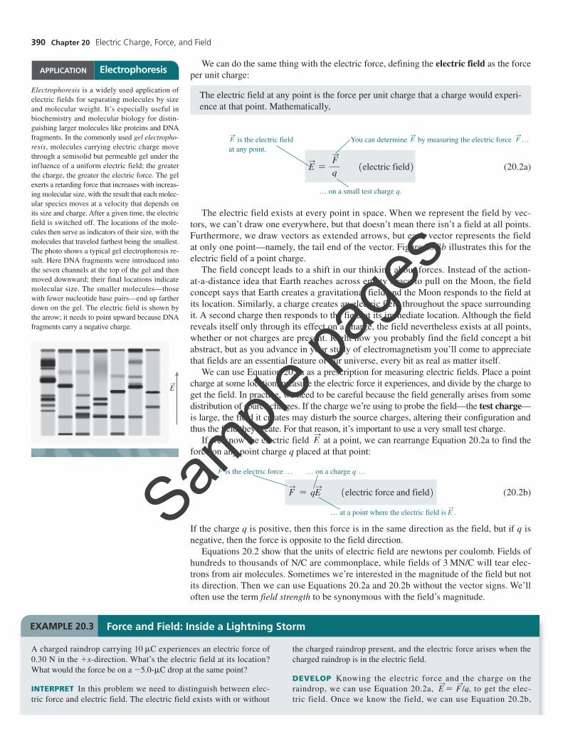
Electrophoresis is a widely used application of electric fields for separating molecules by size and molecular weight. It’s especially useful in biochemistry and molecular biology for distin-guishing larger molecules like proteins and DNA fragments. In the commonly used gel electropho-resis, molecules carrying electric charge move through a semisolid but permeable gel under the influence of a uniform electric field; the greater the charge, the greater the electric force. The gel exerts a retarding force that increases with increas-ing molecular size, with the result that each molec-ular species moves at a velocity that depends on its size and charge. After a given time, the electric field is switched off. The locations of the mole-cules then serve as indicators of their size, with the molecules that traveled farthest being the smallest. The photo shows a typical gel electrophoresis re-sult. Here DNA fragments were introduced into the seven channels at the top of the gel and then moved downward; their final locations indicate molecular size. The smaller molecules—those with fewer nucleotide base pairs—end up farther down on the gel. The electric field is shown by the arrow; it needs to point upward because DNA fragments carry a negative charge.

ES

APPLICATION Electrophoresis

FS

= qES 1electric force and field2 (20.2b)

FS

is the electric force … … on a charge q …

… at a point where the electric field is ES

.

A charged raindrop carrying 10 mC experiences an electric force of 0.30 N in the +x-direction. What’s the electric field at its location? What would the force be on a -5.0@mC drop at the same point?

INTERPRET In this problem we need to distinguish between elec-tric force and electric field. The electric field exists with or without

the charged raindrop present, and the electric force arises when the charged raindrop is in the electric field.

DEVELOP Knowing the electric force and the charge on the raindrop, we can use Equation 20.2a, E

S= F

S/q, to get the elec-

tric field. Once we know the field, we can use Equation 20.2b,

Force and Field: Inside a Lightning StormEXAMPLE 20.3

If the charge q is positive, then this force is in the same direction as the field, but if q is negative, then the force is opposite to the field direction.

Equations 20.2 show that the units of electric field are newtons per coulomb. Fields of hundreds to thousands of N/C are commonplace, while fields of 3 MN/C will tear elec-trons from air molecules. Sometimes we’re interested in the magnitude of the field but not its direction. Then we can use Equations 20.2a and 20.2b without the vector signs. We’ll often use the term field strength to be synonymous with the field’s magnitude.

The electric field at any point is the force per unit charge that a charge would experi-ence at that point. Mathematically,

ES

=FS

q 1electric field2 (20.2a)

ES

is the electric field at any point.

You can determine ES

by measuring the electric force FS

…

… on a small test charge q.

We can do the same thing with the electric force, defining the electric field as the force per unit charge:

M20_WOLF1186_04_GE_C20.indd 390 19/05/20 1:02 AM

Sample

page

s

20.4 Fields of Charge Distributions 391

The Field of a Point ChargeOnce we know the field of a charge distribution, we can calculate its effect on other charges. The simplest charge distribution is a single point charge. Coulomb’s law gives the force on a test charge qtest located a distance r from a point charge q: F

S= 1kqqtest/r

22rn, where rn is a unit vector pointing away from q. The electric field arising from q is the force per unit charge, or

THE FIELD IS INDEPENDENT OF THE TEST CHARGE Does the electric field in this example point in the -x-direction when the charge is negative? No. The field is independent of the particular charge experiencing that field. Here the electric field points in the +x-direction no matter what charge you put in the field. For a positive charge, the force qE

S points in

the same direction as the field; for a negative charge, q 6 0, the force is opposite the field.

Since it’s so closely related to Coulomb’s law for the electric force, we also refer to Equation 20.3 as Coulomb’s law. The equation contains no reference to the test charge qtest because the field of q exists independently of any other charge. Since rn always points away from q, the direction of E

Sis radially outward if q is positive and radially inward if q

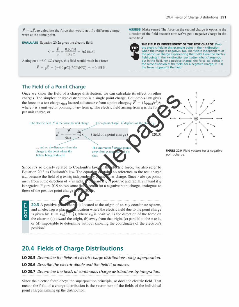
is negative. Figure 20.9 shows some field vectors for a negative point charge, analogous to those of the positive point charge in Fig. 20.8b.

FIGURE 20.9 Field vectors for a negative point charge.

FS

= qES

, to calculate the force that would act if a different charge were at the same point.

EVALUATE Equation 20.2a gives the electric field:

ES

=FS

q=

0.30in N10 mC

= 30in kN/C

Acting on a -5.0@mC charge, this field would result in a force

FS

= qES

= 1-5.0 mC2130in kN/C2 = -0.15in N

ASSESS Make sense? The force on the second charge is opposite the direction of the field because now we’ve got a negative charge in the same field.

20.3 A positive point charge is located at the origin of an x–y coordinate system, and an electron is placed at a location where the electric field due to the point charge is given by E

S= E01 in + jn2, where E0 is positive. Is the direction of the force on

the electron (a) toward the origin, (b) away from the origin, (c) parallel to the x-axis, or (d) impossible to determine without knowing the coordinates of the electron’s position?

GO

T IT

?

20.4 Fields of Charge DistributionsLO 20.5 Determine the fields of electric charge distributions using superposition.

LO 20.6 Describe the electric dipole and the field it produces.

LO 20.7 Determine the fields of continuous charge distributions by integration.

Since the electric force obeys the superposition principle, so does the electric field. That means the field of a charge distribution is the vector sum of the fields of the individual point charges making up the distribution:

ES

=FS

qtest=

kq

r2 rn 1field of a point charge2 (20.3)

The electric field ES

is the force per unit charge. For a point charge, ES

depends on the charge q …

… and on the distance r from the charge to the point where the field is being evaluated.

The unit vector rn always points away from q, regardless of q’s sign.

¯˙

M20_WOLF1186_04_GE_C20.indd 391 19/05/20 1:02 AM

Sample

page

s


Here the ES

i>s are the fields of the point charges qi located at distances ri from the point where we’re evaluating the field—called, appropriately, the field point. The rni>s are unit vectors pointing from each point charge toward the field point. In principle, Equation 20.4 gives the electric field of any charge distribution. In practice, the process of summing the individual field vectors is often complicated unless the charge distribution contains rela-tively few charges arranged in a symmetric way.

Finding electric fields using Equation 20.4 involves the same strategy we intro-duced for finding the electric force; the only difference is that there’s no charge to experience the force. The first step then involves identifying the field point. We still need to find the appropriate unit vectors and form the vector sum in Equation 20.4. Example 20.4 shows how this is done.

Sometimes we’re interested in finding not the electric field but a point or points where the field is zero. Conceptual Example 20.2 explores such a case.

Two protons are 3.6 nm apart. Find the electric field at a point be-tween them, 1.2 nm from one of the protons. Then find the force on an electron at this point.

INTERPRET We follow our electric-force strategy, except that instead of identifying the charge experiencing the force, we identify the field point as being 1.2 nm from one proton. The source charges are the two protons; they produce the field we’re interested in.

DEVELOP Let’s have the protons define the x-axis, as drawn in Fig. 20.10. Then the unit vector rn1 from the left-hand proton toward the field point (which we’ve marked P) is + in, while rn2 from the right-hand proton toward P is - in.

EVALUATE We now evaluate the field at P using Equation 20.4:

ES

= ES

1 + ES

2 =ke

r12 in +

ke

r22 1- in2 = ke a 1

r12 -

1

r22 b in

We wrote e for q here because the protons’ charge is the elementary charge.

Using e = 1.6 * 10-19 C, r1 = 1.2 nm, and r2 = 2.4 nm gives ES

= 750in MN/C. An electron at P will therefore experience a force FS

= qE = -eE = -0.12in nN.

ASSESS Make sense? The field points in the positive x-direction, re-flecting the fact that P is closer to the left-hand proton with its stron-ger field at P. The force on the electron, on the other hand, is in the -x-direction; that’s because the electron is negative (we used q = -e for its charge), so the force it experiences is opposite the field. That field of almost 1 GN/C sounds huge—but that’s not unusual at the mi-croscopic scale, where we’re close to individual elementary particles.

Finding the Field: Two ProtonsEXAMPLE 20.4

Unit vectors point from the sourcecharges toward the field point P.

FIGURE 20.10 Finding the electric field at P.

CONCEPTUAL EXAMPLE 20.2 Zero Field, Zero Force

A positive charge +2Q is located at the origin, and a negative charge -Q is at x = a. In which region of the x-axis is there a point where the force on a test charge—and therefore the electric field—is zero?

INTERPRET We’re asked to locate qualitatively a point where the field is zero. Our sketch of the situation, Fig. 20.11, shows that the two charges divide the x-axis into three regions: (1) to the left of 2Q (x 6 0), (2) between the charges (0 6 x 6 a), and (3) to the right of -Q (x 7 a). We need to determine which region could include a point where the electric force on a test charge is zero.

EVALUATE Consider what would happen to a positive test charge placed in each of these three regions. Anywhere in region (1), the test charge is closer to the charge with greater magnitude (2Q). That charge dominates throughout region (1), where our test charge would experi-ence a repulsive force (to the left). The electric field, then, can’t be zero in region (1). Between the two charges, the repulsive force from 2Q on a positive test charge points to the right; so does the attractive force from -Q. The field, therefore, can’t be zero in region (2). That leaves region (3). Could the field be zero here? Put a positive test charge very close to -Q, and it experiences an attractive force toward the left. But far away, the distance between 2Q and -Q becomes negligible. The

ES

= ES

1 + ES

2 + ES

3 + g = ai

ES

i = a

i

kqi

ri2 rni (20.4)


of a distribution of point charges…

… is the sum of the fields of the individual point charges.

˙ ¯˙ ¯˙

M20_WOLF1186_04_GE_C20.indd 392 19/05/20 1:02 AM

Sample

page

s

FIGURE 20.11 Where is the electric field zero? We’ve marked the an-swer, at x = 3.4a.

The Electric DipoleOne of the most important charge distributions is the electric dipole, consisting of two point charges of equal magnitude but opposite sign. Many molecules are essentially di-poles, so understanding the dipole helps explain molecular behavior (Fig. 20.12). During contraction the heart muscle becomes essentially a dipole, and physicians performing electrocardiography are measuring, among other things, the strength and orientation of that dipole. Antennas used in wireless communications—including radio, TV, wifi, and cellphones—are often based on the dipole configuration.

O-

H+

H+

-

+

≃FIGURE 20.12 A water molecule behaves like an electric dipole. Its net charge is zero, but regions of positive and nega-tive charge are separated.

fields of both charges drop off as the inverse square of the distance, so at large distances the field of the stronger charge will dominate. Therefore there is a point somewhere to the right of -Q where the force on a test charge, and therefore the electric field, will be zero.

ASSESS This answer is consistent with our insight from Example 20.2 that when we get far from a charge distribution, it begins to re-semble a point charge with the net charge of the distribution. Here that net charge is 2Q - Q = +Q, so at large distances we should indeed have a field pointing away from the charge distribution—and that’s to the right in region (3). Although we considered a positive test charge, you’ll reach the same conclusion with a negative test charge.

MAKING THE CONNECTION Find an expression for the position where the electric field in this example is zero.

EVALUATE In Fig. 20.11, we’ve taken the origin at 2Q, so at any po-sition x in region (3) we’re a distance x from 2Q and a distance x-a from -Q. Since we’re to the right of both charges, the unit vector in Equation 20.3 for the point-charge field—a vector that always points away from the point charge—becomes + in for both charges. Applying Equation 20.3, E

S= 1kq/r22rn, for the fields of the two charges and

summing gives

ES

=k12Q2

x2 in +k1-Q21x - a22 in

If we set this expression to zero, we can cancel k, Q, and in; invert-ing both sides of the remaining equation gives x2/2 = 1x - a22. Finally, taking the square root and solving for x gives the answer:

x = a22/122 - 12 ≃ 3.4a. As a check, note that this point does indeed lie to the right of x = a. We’ve marked this point in Fig. 20.11.

A molecule may be modeled approximately as a positive charge q at x = a and a negative charge -q at x = -a. Evaluate the electric field on the y-axis, and find an approximate expression valid at large dis-tances 1 � y � W a2.

INTERPRET Here’s another example where we’ll use our strategy in applying Equation 20.4 to calculate the field of a charge distribution. We identify the field point as being anywhere on the y-axis and the source charges as being {q.

DEVELOP Figure 20.13 is our drawing. The individual unit vectors point from the two charges toward the field point, but the negative charge contributes a field opposite its unit vector; we’ve indicated the individual fields in Fig. 20.13. Here symmetry makes the y- components cancel, giving a net field in the -x-direction. So we need only the x-components of the unit vectors, which Fig. 20.13 shows are rnx- = a/r for the negative charge at -a and rnx+ = -a/r for the positive charge at a.

EVALUATE We then evaluate the field using Equation 20.4:

ES

=k1-q2

r2 aarb in +

kq

r2 a-arb in = -

2kqa

1a2 + y223/2 in

where in the last step we used r = 2a2 + y2. For � y � W a we can neglect a2 compared with y2, giving

ES

≃ -2kqa

� y � 3 in 1 � y � W a2

The Electric Dipole: Modeling a MoleculeEXAMPLE 20.5

Here’s the field point.

+a is the x-component ofthe displacementr- from -q to thefield point c

cso the x-component ofthe unit vector from -qis rx- = a>r c

cand the x-componentof the displacement from+q is -a, so rx+ = -a>r.nn

u

FIGURE 20.13 Finding the field of an electric dipole.

(continued )


M20_WOLF1186_04_GE_C20.indd 393 19/05/20 1:02 AM

Sample

page

s


You can show in Problem 54 that the field on the dipole axis is given by

ES

=2kp

� x � 3 in a dipole fieldfor � x � W a, on axis

b (20.6b)

Because the dipole isn’t spherically symmetric, its field depends not only on distance but also on orientation; for instance, Equations 20.6 show that the field along the dipole axis at a given distance is twice as strong as along the bisector. So it’s important to know the orientation of a dipole in space, and therefore we generalize our definition of the di-pole moment to make it a vector of magnitude p = qd in the direction from the negative toward the positive charge (Fig. 20.14).

Example 20.5 shows that the dipole field at large distances decreases as the inverse cube of distance. Physically, that’s because the dipole has zero net charge. Its field arises entirely from the slight separation of two opposite charges. Because of this separation, the dipole field isn’t exactly zero, but it’s weaker and more localized than the field of a point charge. Many complicated charge distributions exhibit the essential characteristic of a dipole—that is, they’re neutral but consist of separated regions of positive and negative charge—and at large distances, such distributions all have essentially the same field configuration.

At large distances the dipole’s physical characteristics q and a enter the equation for the electric field only through the product qa. We could double q and halve a, and the di-pole’s electric field would remain unchanged. At large distances, therefore, a dipole’s elec-tric properties are characterized completely by its electric dipole moment p, defined as the product of the charge q and the separation d between the two charges making up the dipole:

p = qd 1dipole moment2 (20.5)

In Example 20.5 the charge separation was d = 2a, so there the dipole moment was p = 2aq. In terms of the dipole moment, the field in Example 20.5 can then be written

ES

= -kp

� y � 3 in adipole field for � y � W a,on perpendicular bisector

b (20.6a)

pu

+q

-q

d

-

+

FIGURE 20.14 The dipole moment vector pS has magnitude p = qd and points

from the negative toward the positive charge.

20.4 Far from a charge distribution, you measure an electric field strength of 800 N/C. What will the field strength be if you double your distance from the charge distribution, if the distribution consists of (1) a point charge or (2) a dipole?

GO

T IT

?

Continuous Charge DistributionsAlthough any charge distribution ultimately consists of pointlike electrons and protons, it would be impossible to sum all the field vectors from the 1023 or so particles in a typical piece of matter. Instead, it’s convenient to make the approximation that charge is spread continuously over the distribution. If the charge distribution extends throughout a volume, we describe it in terms of the volume charge density r, with units of C/m3. For charge distributions spread over surfaces or lines, the corresponding quantities are the surface charge density s 1C/m22 and the line charge density l 1C/m2.

ASSESS Make sense? The dipole has no net charge, so at large distances its field can’t have the inverse-square drop-off of a point-charge field. Instead the dipole field falls faster, here as 1/ � y � 3. Note that we were careful to put absolute value signs on y3; that way, our result applies for both positive and negative values of y.

APPROXIMATIONS Making approximations requires care. Here we’re basically asking for the field when y is so large that a is negligible compared with y. So we neglect a2 compared with y2 when the two are summed, but we don’t neglect a when it appears in the numerator, where it isn’t being directly compared with y.

M20_WOLF1186_04_GE_C20.indd 394 19/05/20 1:02 AM

Sample

page

s


ES

= LdES

= Lk dq

r2 rn afield of a continuouscharge distribution

b (20.7)


of a continuous distribution of charges …

dq is an infinitesimal charge element.

rn is a unit vector that points away from dq, regardless of its sign.

… is determined by integrating the fields dE

S of infinitesimal charge elements dq.

r is the distance from dq to the point where the field is being evaluated.

The limits of this integral include the entire charge distribution.Calculating the field of a continuous charge distribution involves the same strategy

we’ve already used: We identify the field point and the source charges—although now the source is a continuous charge distribution. Summing the individual field contributions now presents us with an integral, and that means writing the unit vectors rn and distances r in terms of coordinates over which we can integrate. Setting up the integral involves the same strategy we outlined in Chapter 9 to find the center of mass of a continuous distribution of matter, and used again in Chapter 10 to find rotational inertias.

rnrn

rnESP

dq

dqdq

rr

r

Charge distribution

dES

dES

dES

FIGURE 20.15 The electric field at P is the vector sum of the fields dE

S arising from

the individual charge elements dq, each calculated using the appropriate distance r and unit vector rn.

A ring of radius a carries a charge Q distributed evenly over the ring. Find an expression for the electric field at any point on the axis of the ring.

INTERPRET We identify the field point as lying anywhere on the ring’s axis, and the source charge as the entire ring.

DEVELOP Let’s take the x-axis to coincide with the ring axis, with the center of the ring at x = 0 (Fig. 20.16). The figure shows that the y-components of the field contributions from pairs of charge elements on opposite sides of the ring cancel; therefore, the net field points in the +x-direction (for x 7 0) and we need only the x-components of the unit vectors. Those are the same for all unit vectors—namely, rnx = x/r.

EVALUATE We’re now ready to set up the integral in Equation 20.7. Here each charge element contr ibutes the same amount dEx = 1k dq/r22rnx = 1k dq/r221x/r2 to the field. Figure 20.16 shows

that r = 2x2 + a2 = 1x2 + a221/2, so the integral becomes

E = Lring dEx = Lring

kx dq

1x2 + a223/2 =kx

1x2 + a223/2 Lring dq

The last step follows because we have a fixed field point P, so its coor-dinate x is a constant for the integration. But the remaining integral is just the sum of all the charge elements on the ring—namely, the total charge Q. So our result becomes

E =kQx

1x2 + a223/2 (on@axis field, charged ring)

This is the magnitude; the direction is along the x-axis, away from the ring if Q is positive and toward it if Q is negative.

ASSESS Make sense? At x = 0 the field is zero. A charge placed at the ring center is pulled (or pushed) equally in all directions—no net force, so no electric field. But for x W a, we get E = kQ/x2—just what we expect for a point charge Q. As always, a finite-sized charge distribution looks like a point charge at large distances. Problem 73 shows how you can use the result of this example to find the electric field on the axis of a charged disc, and Problem 75 shows that, once again, the field at large distances becomes that of a point charge.

Evaluating the Field: A Charged RingEXAMPLE 20.6

FIGURE 20.16 The electric field of a charged ring points along the ring axis, since field components perpendicular to the axis cancel in pairs.

To calculate the field of a continuous charge distribution, we divide the charged re-gion into very many small charge elements dq, each small enough that it’s essentially a point charge. Each dq then produces an electric field dE

S given by Equation 20.3:

dES

= 1k dq/r22rn. We then form the vector sum of all the dES>s (Fig. 20.15). In the limit of

infinitely many infinitesimally small dq’s and their corresponding dES>s, that sum becomes

an integral and we have

M20_WOLF1186_04_GE_C20.indd 395 19/05/20 1:02 AM

Sample

page

s


A long, straight electric power line coincides with the x-axis and car-ries a uniform line charge density l (unit: C/m). Find the electric field on the y-axis using the approximation that the wire is infinitely long.

INTERPRET We identify the field point as being a distance y from the wire, and the source charge as the whole wire.

DEVELOP Figure 20.17 is our drawing, showing a coordinate system with the field point P along the y-axis. We divide the wire into small charge elements dq and note that field contributions from two such el-ements dq on opposite sides of the y-axis contribute fields dE

S whose

x-components cancel. Then we need only the y-component of each unit vector, and Figure 20.17 shows that’s rny = y/r, where r = 2x2 + y2.

EVALUATE We’re now ready to set up the integral in Equation 20.7. As described in Chapter 9’s integral strategy, we need to relate dq to a geometric variable so we can do the integral. Here our wire has charge density l C/m, so if a charge element has length dx, then its charge is dq = l dx. Putting all this together gives the y-component of the field from an arbitrary dq anywhere on the wire:

dEy =k dq

r2 rny =kl dx

r2 y

r=

kly

1x2 + y223/2 dx

where we used r = 2x2 + y2. Since the x-components cancel, we can sum—that is, integrate—the y-components to get the net field:

E = Ey = L+∞

-∞

kly dx

1x2 + y223/2 = klyL+∞

-∞

dx

1x2 + y223/2

= kly c x

y22x2 + y2d

-∞

+∞= kly c 1

y2 - a-1

y2 b d =2kl

y

Here we used the integral table in Appendix A and applied the limits x = {∞ . Our result is the field’s magnitude; the direction is away from the line for positive l and toward the line for negative l.

ASSESS Make sense? For an infinite line there’s nothing to favor one direction along the line over another, so the only way the field can point is radially, away from or toward the line (Fig. 20.18). And because the line is infinite, it never resembles a point no matter how far away we are. As a result the field falls more slowly than the field of a point charge—in this case, as 1/y. If we let r designate the ra-dial distance from the line rather than the diagonal in Fig. 20.17, then the field decreases as 1/r. An infinite line is impossible, but our result holds approximately for finite lines of charge as long as we’re much closer to the line than its length, and not near an end. Far from a finite line, on the other hand, its field will resemble that of a point charge. You can explore the finite charged line in Problem 72.

Line Charge: A Power Line’s FieldWorked Example with Variation Problems

EXAMPLE 20.7

This is the y-component of thedisplacement rfrom dq to P c

cso the y-component ofthe unit vector ris y>r.

n

u

FIGURE 20.17 The field of a charged line is the vector sum of the fields dE

S from all the individual charge elements dq along the line.

FIGURE 20.18 Field vectors for an infinite line of pos-itive charge point radially outward, with magnitude decreasing inversely with distance.

20.5 Matter in Electric FieldsLO 20.8 Determine the motion of charged particles in electric fields.

LO 20.9 Determine forces and torques on electric dipoles in electric fields.

Electric fields give rise to forces on charged particles. Because matter consists of such particles, much of the behavior of matter is fundamentally determined by electric fields.

Point Charges in Electric FieldsThe motion of a single charge in an electric field is governed by the definition of the elec-tric field, F

S= qE

S, and Newton’s law, F

S= ma

!. Combining these equations gives the

acceleration of a particle with charge q and mass m in an electric field ES

:

a!

=qm

ES

(20.8)

M20_WOLF1186_04_GE_C20.indd 396 19/05/20 1:02 AM

Sample

page

s

20.5 Matter in Electric Fields 397

This equation shows that it’s the charge-to-mass ratio, q/m, that determines a particle’s re-sponse to an electric field. Electrons, nearly 2000 times less massive than protons but car-rying the same charge, are readily accelerated by electric fields. Many practical devices, from X-ray machines to fluorescent lights, use electrons accelerated in electric fields.

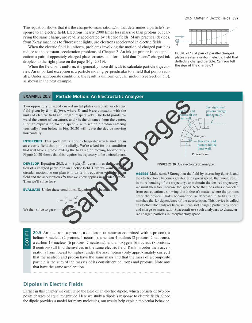
When the electric field is uniform, problems involving the motion of charged particles reduce to the constant-acceleration problems of Chapter 2. An ink-jet printer is one appli-cation; a pair of oppositely charged plates creates a uniform field that “steers” charged ink droplets to the right place on the page (Fig. 20.19).

When the field isn’t uniform, it’s generally more difficult to calculate particle trajecto-ries. An important exception is a particle moving perpendicular to a field that points radi-ally. Under appropriate conditions, the result is uniform circular motion (see Section 5.3), as shown in the next example.

+ + + + + + + +

- - - - - - - -q

FIGURE 20.19 A pair of parallel charged plates creates a uniform electric field that deflects a charged particle. Can you tell the sign of the charge q?

Two oppositely charged curved metal plates establish an electric field given by E = E01b/r2, where E0 and b are constants with the units of electric field and length, respectively. The field points to-ward the center of curvature, and r is the distance from the center. Find an expression for the speed v with which a proton entering vertically from below in Fig. 20.20 will leave the device moving horizontally.

INTERPRET This problem is about charged-particle motion in an electric field that points radially. We’re asked for the condition that will have a proton exiting the field region moving horizontally. Figure 20.20 shows that this requires its trajectory to be a circular arc.

DEVELOP Equation 20.8, a!

= 1q/m2 ES

, determines the accelera-tion of a charged particle in an electric field. Here we want uniform circular motion, so our plan is to write this equation with the given field and the acceleration v2/r that we know applies in circular motion. Then we’ll solve for v.

EVALUATE Under these conditions, Equation 20.8 becomes

a =v2

r=

eEm

=em

E0

br

We then solve to get v = 1eE0b/m.

ASSESS Make sense? Strengthen the field by increasing E0 or b, and the electric force becomes greater. For a given speed, that would result in more bending of the trajectory; to maintain the desired trajectory, we must therefore increase the speed. Note that the radius r canceled from our equations, showing that it doesn’t matter where the protons enter the device. That’s because the 1/r decrease in field strength matches the 1/r dependence of the acceleration. This device is called an electrostatic analyzer because it can sort charged particles by speed and charge-to-mass ratio. Spacecraft use such analyzers to character-ize charged particles in interplanetary space.

Particle Motion: An Electrostatic AnalyzerEXAMPLE 20.8

ES

Too fast, and protons hit theouter wall.

Just right, and protons emergehorizontally.

Too slow, andprotons hit theinner wall.

Analyzer

Proton beam

FIGURE 20.20 An electrostatic analyzer.

20.5 An electron, a proton, a deuteron (a neutron combined with a proton), a helium-3 nucleus (2 protons, 1 neutron), a helium-4 nucleus (2 protons, 2 neutrons), a carbon-13 nucleus (6 protons, 7 neutrons), and an oxygen-16 nucleus (8 protons, 8 neutrons) all find themselves in the same electric field. Rank in order their accel-erations from lowest to highest under the assumption (only approximately correct) that the neutron and proton have the same mass and that the mass of a composite particle is the sum of the masses of its constituent neutrons and protons. Note any that have the same acceleration.

GO

T IT

?

Dipoles in Electric FieldsEarlier in this chapter we calculated the field of an electric dipole, which consists of two op-posite charges of equal magnitude. Here we study a dipole’s response to electric fields. Since the dipole provides a model for many molecules, our results help explain molecular behavior.

M20_WOLF1186_04_GE_C20.indd 397 19/05/20 1:02 AM

Sample

page

s

Figure 20.21 shows a dipole with charges {q separated a distance d, located in a uni-form electric field. The dipole moment vector p

! has magnitude qd and points from the

negative to the positive charge (recall Fig. 20.14). Since the field is uniform, it’s the same at both ends of the dipole. Since the dipole charges are equal in magnitude but opposite in sign, they experience equal but opposite forces {qE

S—and therefore there’s no net force

on the dipole.However, Fig. 20.21 shows that the dipole does experience a torque that tends to align

it with the field. In Chapter 11 we described torque as the cross product of the position vector with the force: t

!= r

!* F

S, where the magnitude of the torque vector is rF sin u

and its direction is given by the right-hand rule. Figure 20.21 thus shows that the torque about the center of the dipole due to the force on the positive charge has magnitude t+ = rF sin u = 11

2 d21qE2 sin u. The torque associated with the negative charge has the same magnitude, and both torques are in the same direction since both tend to rotate the dipole clockwise. Thus the net torque has magnitude t = qdE sin u. Applying the right-hand rule shows that this torque is into the page. But qd is the magnitude of the dipole moment p

!, and Fig. 20.21 shows that u is the angle between the dipole moment vector and

the electric field ES

; therefore, we can write the torque vectorially as

t!

= p!

* ES 1torque on a dipole2 (20.9)

Because of this torque, the electric field does work on a dipole as it rotates. The electric force is conservative, so that work results in a change in potential energy. In Chapter 7 we defined potential-energy change as the negative of the work done by a conservative force: ∆U = -W. Here we’re dealing with rotational motion, and Equation 10.19 shows that the work done in a rotation from angular position u1 to u2 is given by W = 1u2

u1t du.

Figure 20.21 shows that we’re taking u = 0 when the dipole is aligned with the field. The figure also shows that the direction of increasing u is counterclockwise or, in terms of ro-tational vectors, out of the page. The torque, in contrast, is clockwise or, vectorially, into the page. Thus the sign of the torque is opposite the angular change, so we need to write t = -pE sin u in the integral for the work. Let’s now consider a dipole that’s initially per-pendicular to the field, so u1 = p/2. Then the work done by the electric force as the dipole rotates to an arbitrary angle u becomes

W = Lu

p/2t du = L

u

p/21-pE sin u2 du = -pE3- cos u4 up/2 = pE cos u

The potential-energy change is the negative of this work, and we note that pE cos u can be expressed as the dot product p

! # E

S, so we can write the potential energy as

U = -p! # E

S (20.10)

where U = 0 corresponds to the dipole at right angles to the field.When the electric field isn’t uniform, the charges at opposite ends of the dipole expe-

rience forces that differ in magnitude and/or aren’t exactly opposite in direction. Then the dipole experiences a net force as well as a torque (Fig. 20.22). An important instance of this effect is the force on a dipole in the field of another dipole (Fig. 20.23). Because the dipole field falls off rapidly with distance and because the dipole responding to the field has closely spaced charges of equal magnitude but opposite sign, the dipole–dipole force is quite weak and falls extremely rapidly with distance. This weak force, which Fig. 20.23 shows to be attractive, is partly responsible for the van der Waals interaction between gas molecules that we mentioned in Chapter 17.

Conductors, Insulators, and DielectricsBulk matter contains vast numbers of point charges—namely, electrons and protons. In some matter—notably metals, ionic solutions, and ionized gases—individual charges are free to move throughout the material. In these conductors, the application of an electric field results in the ordered motion of electric charge that we call electric current. We’ll consider conductors and current in later chapters.

E2S

E1S

F2S

FnetSF1

S

-

+

FIGURE 20.22 When the electric field dif-fers in magnitude or direction at the two ends of the dipole, the dipole experiences a nonzero net force as well as a torque.

pu

ES

F-S

F+S

-

+u

Torque rotatesdipole clockwise.

d

FIGURE 20.21 A dipole in a uniform electric field experiences a torque but no net force.

E+S

F+S

E-S

F-S

- -+ +

Force on negative end of B is stronger; hencenet force is toward A.

A B

FIGURE 20.23 Dipole B aligns with the field of dipole A and then experiences a net force toward A.


M20_WOLF1186_04_GE_C20.indd 398 19/05/20 1:02 AM

Sample

page

s

20.5 Matter in Electric Fields 399

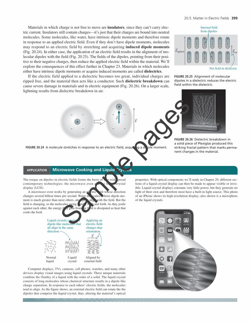
Materials in which charge is not free to move are insulators, since they can’t carry elec-tric current. Insulators still contain charges—it’s just that their charges are bound into neutral molecules. Some molecules, like water, have intrinsic dipole moments and therefore rotate in response to an applied electric field. Even if they don’t have dipole moments, molecules may respond to an electric field by stretching and acquiring induced dipole moments (Fig. 20.24). In either case, the application of an electric field results in the alignment of mo-lecular dipoles with the field (Fig. 20.25). The fields of the dipoles, pointing from their posi-tive to their negative charges, then reduce the applied electric field within the material. We’ll explore the consequences of this effect further in Chapter 23. Materials in which molecules either have intrinsic dipole moments or acquire induced moments are called dielectrics.

If the electric field applied to a dielectric becomes too great, individual charges are ripped free, and the material then acts like a conductor. Such dielectric breakdown can cause severe damage in materials and in electric equipment (Fig. 20.26). On a larger scale, lightning results from dielectric breakdown in air.

pu

ES

FIGURE 20.24 A molecule stretches in response to an electric field, acquiring a dipole moment.

The torque on dipoles in electric fields forms the basis of two widespread contemporary technologies: the microwave oven and the liquid-crystal display (LCD).

A microwave oven works by generating an electric field whose direction changes several billion times per second. Water molecules, whose dipole mo-ment is much greater than most others, attempt to align with the field. But the field is changing, so the molecules swing rapidly back and forth. As they jostle against each other, the energy they gain from the field is dissipated as heat that cooks the food.

ES

Liquid crystals consist ofdipole-like molecules thatall align in the same direction.

Applying anelectric fieldchanges thatorientation.

Normalliquid

Liquidcrystal

Aligned byexternal field

Computer displays, TVs, cameras, cell phones, watches, and many other devices display visual images using liquid crystals. These unique materials combine the fluidity of a liquid with the order of a solid. The liquid crystal consists of long molecules whose chemical structure results in a dipole-like charge separation. In response to each others’ electric fields, the molecules tend to align. As the figure shows, an external electric field can rotate the the dipoles that comprise the liquid crystal, thus, altering the material’s optical

properties. With optical components we’ll study in Chapter 29, different sec-tions of a liquid-crystal display can then be made to appear visible or invis-ible. Liquid-crystal displays consume very little power, but they generate no light of their own and therefore most have a built-in light source. This photo of an iPhone shows its high-resolution display; also shown is a microphoto of the liquid crystals.

APPLICATION Microwave Cooking and Liquid Crystals

EnetSEapplied

S -

+

-

+

-

+

-

+

-

+

-

+

-

+

-

+

-

+

-

+

-

+

-

+

Internal fieldfrom dipoles

Net field in dielectric

FIGURE 20.25 Alignment of molecular dipoles in a dielectric reduces the electric field within the dielectric.

FIGURE 20.26 Dielectric breakdown in a solid piece of Plexiglas produced this striking fractal pattern that marks perma-nent changes in the material.

M20_WOLF1186_04_GE_C20.indd 399 19/05/20 1:02 AM

Sample

page

s

Key Concepts and Equations

Chapter 20 Summary

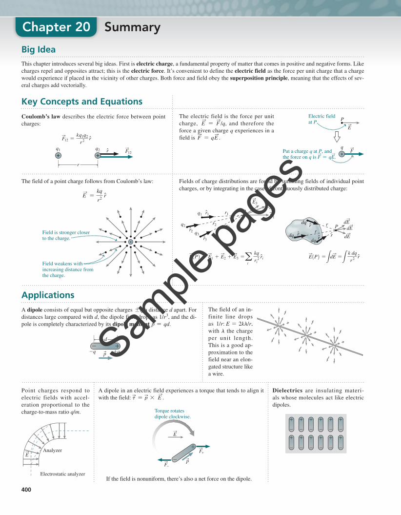
Big IdeaThis chapter introduces several big ideas. First is electric charge, a fundamental property of matter that comes in positive and negative forms. Like charges repel and opposites attract; this is the electric force. It’s convenient to define the electric field as the force per unit charge that a charge would experience if placed in the vicinity of other charges. Both force and field obey the superposition principle, meaning that the effects of sev-eral charges add vectorially.

The electric field is the force per unit charge, E

S= F

S/q, and therefore the

force a given charge q experiences in a field is F

S= qE

S.

ApplicationsA dipole consists of equal but opposite charges {q a distance d apart. For distances large compared with d, the dipole field drops as 1/r3, and the di-pole is completely characterized by its dipole moment p = qd.

pu

- +d

+q-q

Point charges respond to electric fields with accel-eration proportional to the charge-to-mass ratio q/m.

ES Analyzer

Electrostatic analyzer

ES

FS

Electric fieldat P P

qPut a charge q at P, and the force on q is F = qE.

SS

Coulomb’s law describes the electric force between point charges:

rn

rn

kq1q2

r2

F12S

F12 =

r

q1 q2

S

The field of a point charge follows from Coulomb’s law:

ES

=kq

r2 rn

Field is stronger closerto the charge.

Field weakens withincreasing distance fromthe charge.

Fields of charge distributions are found by summing fields of individual point charges, or by integrating in the case of continuously distributed charge:

k dqr2

kqri

2ai

E1

E2

E3

r1q1

q2

q3

r2 r3dE

dE

dE

P

P

dq

dqdq

rr

r

E1P2 = E1 + E2 + E3 = ri E1P2 = dE = rL L

r1n

r2n

r3n

n n

rn

rnrn

SS

S

S S S S

S

S

S

S S

The field of an in-finite line drops as 1/r: E = 2kl/r, with l the charge per unit length. This is a good ap-proximation to the field near an elon-gated structure like a wire.

A dipole in an electric field experiences a torque that tends to align it with the field: t

!= p

!* E

S.

pu

ES

Torque rotatesdipole clockwise.

-

+F+S

F-S

If the field is nonuniform, there’s also a net force on the dipole.

Dielectrics are insulating materi-als whose molecules act like electric dipoles.

-

+

-

+

-

+

-

+

-

+

-

+

-

+

-

+

-

+

-

+

-

+

-

+

400

M20_WOLF1186_04_GE_C20.indd 400 19/05/20 1:02 AM

Sample

page

s

Exercises and Problems 401

Exercises and Problems

Exercises

Section 20.1 Electric Charge11. Suppose the electron and proton charges differed by one part in

one billion. Estimate the net charge on your body, assuming it contains equal numbers of electrons and protons.

12. A typical lightning flash delivers about 25 C of negative charge from cloud to ground. How many electrons are involved?

13. Protons and neutrons are made from combinations of the two most common quarks, the u quark (charge +2

3 e) and the d quark (charge -1

3 e). How could three of these quarks combine to make (a) a proton and (b) a neutron?

14. Earth carries a net charge of about -5 * 105 C. How many more electrons are there than protons on Earth?

15. As they fly, honeybees may acquire electric charges of about 180 pC. Electric forces between charged honeybees and spider webs can make the bees more vulnerable to capture by spiders. How many electrons would a honeybee have to lose to acquire a charge of +180 pC?

Section 20.2 Coulomb’s Law16. The electron and proton in a hydrogen atom are 52.9 pm apart.

Find the magnitude of the electric force between them.17. An electron at Earth’s surface experiences a gravitational force

meg. How far away can a proton be and still produce the same force on the electron? (Your answer should show why gravity is unimportant on the molecular scale!)

18. You break a piece of Styrofoam packing material, and it releases lots of little spheres whose electric charge makes them stick an-noyingly to you. If two of the spheres carry equal charges and repel with a force of 20 mN when they’re 17 mm apart, what’s the magnitude of the charge on each?

19. A charge q is at the point x = 5 m, y = 0 m. Write expressions for the unit vectors you would use in Coulomb’s law if you were finding the force that q exerts on other charges located at (a) x = 5 m, y = 2.5 m; (b) the origin; and (c) x = 7 m, y = 3.5 m. You’re not given the sign of q. Why doesn’t this matter?

BIO

For Thought and Discussion

1. Conceptual Example 20.1 shows that the gravitational force between an electron and a proton is about 10-40 times weaker than the electric force between them. Since matter consists largely of electrons and protons, why is the gravitational force important at all?

2. A free neutron is unstable and soon decays to other particles, one of them a proton. Must there be others? If so, what electric prop-erties must it or they have?

3. Where in Fig. 20.5 could you put a third charge so it would experience no net force? Would it be in stable or unstable equilibrium?

4. Equation 20.3 gives the electric field of a point charge. Does the direction of (a) rn or (b) E

Sdepend on whether the charge is posi-

tive or negative?5. Is the electric force on a charged particle always in the direction

of the field? Explain.6. Why does a dipole, which has no net charge, produce an electric field?7. The ring in Example 20.6 carries total charge Q, and the point P

is the same distance r = 2x2 + a2 from all parts of the ring. So why isn’t the electric field of the ring just kQ/r2?

8. A spherical balloon is initially uncharged. If you spread positive charge uniformly over the balloon’s surface, would it expand or con-tract? What would happen if you spread negative charge instead?

9. Why should there be a force between two dipoles, which each have zero net charge?

10. Dipoles A and B are both located in the field of a point charge Q, as shown in Fig. 20.27. Does either experience a net torque? A net force? If each dipole is released from rest, qualitatively describe its subsequent motion.

Mastering Physics

BIO Biology and/or medicine-related problems DATA Data problems ENV Environmental problems CH Challenge problems COMP Computer problems

Go to www.masteringphysics.com to access assigned homework and self-study tools such as Dynamic Study Modules, practice quizzes, video solutions to problems, and a whole lot more!

Learning Outcomes After finishing this chapter you should be able to:

LO 20.1 Describe electric charge as a fundamental property of matter.For Thought and Discussion Questions 20.1, 20.2, 20.8; Exercises 20.11, 20.12, 20.13, 20.14, 20.15

LO 20.2 Use Coulomb’s law to calculate the forces between charges.Exercises 20.16, 20.17, 20.18, 20.19, 20.20; Problems 20.44, 20.57, 20.58

LO 20.3 Use the superposition principle to calculate forces involving multiple charges.For Thought and Discussion Question 20.3; Problems 20.46, 20.47, 20.48, 20.49, 20.52

LO 20.4 Describe the concept of electric field.For Thought and Discussion Questions 20.4, 20.5; Exercises 20.21, 20.22, 20.23, 20.24, 20.25, 20.26; Problem 20.50

LO 20.5 Determine the fields of electric charge distributions using superposition.

For Thought and Discussion Question 20.7; Exercises 20.27, 20.28; Problems 20.51, 20.56, 20.59

LO 20.6 Describe the electric dipole and the field it produces.For Thought and Discussion Questions 20.6, 20.9; Problems 20.53, 20.54, 20.55, 20.67, 20.69, 20.70, 20.72

LO 20.7 Determine the fields of continuous charge distributions by integration.Exercises 20.29, 20.30, 20.31; Problems 20.61, 20.64, 20.68, 20.71, 20.73, 20.74, 20.75, 20.76, 20.77, 20.78

LO 20.8 Determine the motion of charged particles in electric fields.Exercises 20.32, 20.33, 20.34, 20.35; Problems 20.60, 20.63

LO 20.9 Determine forces and torques on electric dipoles in electric fields.For Thought and Discussion Questions 20.9, 20.10; Problems 20.62, 20.65, 20.66

- +

- +

A

-q +q

+Q B

-q +q

FIGURE 20.27 For Thought and Discussion 10

M20_WOLF1186_04_GE_C20.indd 401 19/05/20 1:02 AM

Sample

page

s


20. A proton is at the origin and an electron is at the point x = 0.41 nm, y = 0.36 nm. Find the electric force on the proton.

Section 20.3 The Electric Field21. An electron experiences an electric force of 0.61 nN. What’s the

field strength at its location?22. Find the magnitude of the electric force on a 6.0@mC charge in a

50-N/C electric field.23. A 75-nC charge experiences a 144-mN force in a certain electric

field. Find (a) the field strength and (b) the force that a 35@mC charge would experience in the same field.

24. The electric field inside a cell membrane is 8.0 MN/C. What’s the force on a singly charged ion in this field?

25. A -3.0@mC charge experiences a 9.0in@N electric force in a certain electric field. What force would a proton experience in the same field?

26. The electron in a hydrogen atom is 52.9 pm from the proton. At this distance, what’s the strength of the electric field due to the proton?

Section 20.4 Fields of Charge Distributions27. In Fig. 20.28, point P is midway

between the two charges. Find the electric field in the plane of the page (a) 5.0 cm to the left of P, (b) 5.0 cm directly above P, and (c) at P.

28. The water molecule’s dipole moment is 6.17 * 10-30 C #m. What would be the separation distance if the molecule consisted of charges {e? (The effective charge is actually less because H and O atoms share the electrons.)

29. The electric field 22 cm from a long wire carrying a uniform line charge density is 1.9 kN/C. What’s the field strength 38 cm from the wire?

30. Find the line charge density on a long wire if the electric field 39 cm from the wire has magnitude 210 kN/C and points toward the wire.

31. Find the magnitude of the electric field due to a charged ring of radius a and total charge Q on the ring axis at distance a from the ring’s center.

Section 20.5 Matter in Electric Fields32. In his famous 1909 experiment that demonstrated quantization

of electric charge, R. A. Millikan suspended small oil drops in an electric field. With field strength 20 MN/C, what mass drop can be suspended when the drop carries 10 elementary charges?

33. How strong an electric field is needed to accelerate electrons in an X-ray tube from rest to one-tenth the speed of light in a dis-tance of 4.7 cm?

34. A proton moving to the right at 3.3 * 105 m/s enters a region where a 60-kN/C electric field points to the left. (a) How far will the proton get before it momentarily stops? (b) Describe its subsequent motion.

35. An electrostatic analyzer like that of Example 20.8 has b = 7.5 cm. What value of E0 will enable the device to select protons moving at 84 m/s?

Example VariationsThe following problems are based on two examples from the text. Each set of four problems is designed to help you make connections that enhance your understanding of physics and to build your confidence in solving problems that differ from ones you’ve seen before. The first problem in each set is essentially the example problem but with differ-ent numbers. The second problem presents the same scenario as the example but asks a different question. The third and fourth problems repeat this pattern but with entirely different scenarios.

36. Example 20.2: Charges on raindrops vary widely in both magni-tude and sign. Consider a case where the two drops on the x-axis in Example 20.2 are 2.18 mm apart and have charge q = 645 nC, while the third drop is 12.3 mm up the y-axis and has charge Q = -1.87 mC. Find the electric force on the upper drop.

BIO

5.0 cm

P+ 2.0 oC - 2.0 oC

FIGURE 20.28 Exercise 27

37. Example 20.2: Suppose that all three raindrops in Example 20.2 have equal charges and that their positions form an equilateral tri-angle with side 3.36 mm. If the electric force on the upper charge is 96.2 jnN, (a) what’s the magnitude of the charge? (b) Can you determine the sign of the charge from the information given?

38. Example 20.2: (a) Repeat Example 20.2 to find the force on Q, now taking the right-hand charge on the x-axis to be -q . (b) For y W a, how does the force you found in (a) depend on the distance y?

39. Example 20.2: (a) Use calculus to show that the maximum force in the situation of Example 20.2 occurs when y = a>22, and (b) find the magnitude of that maximum force.

40. Example 20.7: A 1.00-km length of power line carries a total charge of 264 mC distributed uniformly over its length. Find the magnitude of the electric field 54.3 cm from the axis of the power line, and not near either end (staying away from the ends means you can approximate the field as that of an infinitely long wire).

41. Example 20.7: A uniformly charged wire is 2.18 m long and 0.15 mm in diameter. You measure the electric field 1.20 cm from the wire’s axis, not near either end, and you find it to be 455 kN/C, pointing toward the wire. Find the total charge on the wire.

42. Example 20.7: A thin rod of length L lies on the x-axis with its center at the origin, as shown in Fig. 20.29. The rod carries charge Q dis-tributed uniformly over its length. (a) Modify the cal-culation of Example 20.7 to find an expression for the electric field at point A in Fig. 20.29, located on the positive y-axis an arbitrary distance y from the origin (but with y large enough to put point A outside the thin rod). (b) Show that your result reduces to the field of a point charge Q when y W L.

43. Example 20.7: A thin rod of length L lies on the x-axis with its center at the origin, as shown in Fig. 20.29. The rod carries charge Q distributed uniformly over its length. (a) Find an ex-pression for the electric field at point B in Fig. 20.29, located on the positive x-axis a distance x from the origin, where x 7 L>2, so that point B is beyond the right end of the rod. (b) Show that your result reduces to the field of a point charge Q when x W L .

Problems44. Two charges, of which one has a magnitude three times as large

as the other’s, are located 14.5 cm apart and experience an attrac-tive force of 156 N. (a) What’s the magnitude of the larger charge? (b) Can you determine the sign of the larger charge?

45. A proton is on the x-axis at x = 1.3 nm. An electron is on the y-axis at y = 0.86 nm. Find the net force the two exert on a helium nucleus (charge +2e) at the origin.

46. A charge 3q is at the origin, and a charge -2q is on the posi-tive x-axis at x = a. Where would you place a third charge so it would experience no net electric force?

47. A negative charge -q lies midway between two positive charges +Q. What must Q be such that the electric force on all three charges is zero?

48. In Fig. 20.30, take q1 = 68 mC, q2 = -34 mC, and q3 = 15 mC. Find the electric force on q3.

49. In Fig. 20.30, take q1 = 21 mC and q2 = 18 mC. If the force on q1 points in the -x-direction, find (a) q3 and (b) the magnitude of the force on q1.

x

y

A

B

L

FIGURE 20.29 Problems 42 and 43

x (m)

y (m)

2

1

1 2 3

q1

q3

q2

FIGURE 20.30 Problems 48 and 49

M20_WOLF1186_04_GE_C20.indd 402 19/05/20 1:02 AM

Sample

page

s

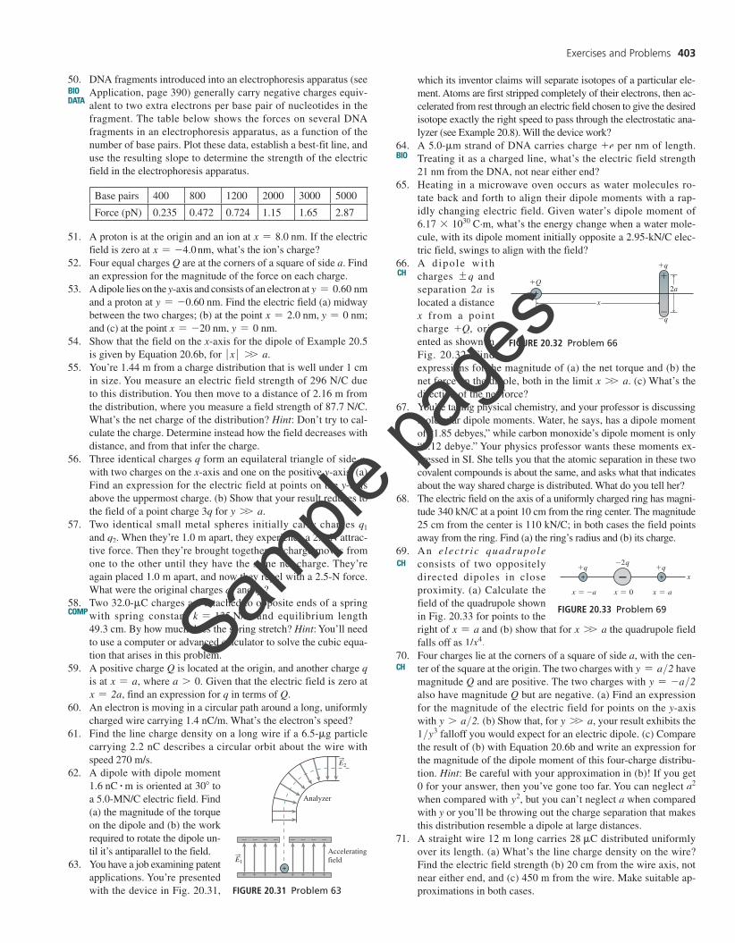
50. DNA fragments introduced into an electrophoresis apparatus (see Application, page 390) generally carry negative charges equiv-alent to two extra electrons per base pair of nucleotides in the fragment. The table below shows the forces on several DNA fragments in an electrophoresis apparatus, as a function of the number of base pairs. Plot these data, establish a best-fit line, and use the resulting slope to determine the strength of the electric field in the electrophoresis apparatus.

Base pairs 400 800 1200 2000 3000 5000

Force (pN) 0.235 0.472 0.724 1.15 1.65 2.87

51. A proton is at the origin and an ion at x = 8.0 nm. If the electric field is zero at x = -4.0 nm, what’s the ion’s charge?

52. Four equal charges Q are at the corners of a square of side a. Find an expression for the magnitude of the force on each charge.

53. A dipole lies on the y-axis and consists of an electron at y = 0.60 nm and a proton at y = -0.60 nm. Find the electric field (a) midway between the two charges; (b) at the point x = 2.0 nm, y = 0 nm; and (c) at the point x = -20 nm, y = 0 nm.

54. Show that the field on the x-axis for the dipole of Example 20.5 is given by Equation 20.6b, for � x � W a.

55. You’re 1.44 m from a charge distribution that is well under 1 cm in size. You measure an electric field strength of 296 N/C due to this distribution. You then move to a distance of 2.16 m from the distribution, where you measure a field strength of 87.7 N/C. What’s the net charge of the distribution? Hint: Don’t try to cal-culate the charge. Determine instead how the field decreases with distance, and from that infer the charge.

56. Three identical charges q form an equilateral triangle of side a, with two charges on the x-axis and one on the positive y-axis. (a) Find an expression for the electric field at points on the y-axis above the uppermost charge. (b) Show that your result reduces to the field of a point charge 3q for y W a.

57. Two identical small metal spheres initially carry charges q1 and q2. When they’re 1.0 m apart, they experience a 2.5-N attrac-tive force. Then they’re brought together so charge moves from one to the other until they have the same net charge. They’re again placed 1.0 m apart, and now they repel with a 2.5-N force. What were the original charges q1 and q2?

58. Two 32.0@mC charges are attached to opposite ends of a spring with spring constant k = 135 N/m and equilibrium length 49.3 cm. By how much does the spring stretch? Hint: You’ll need to use a computer or advanced calculator to solve the cubic equa-tion that arises in this problem.

59. A positive charge Q is located at the origin, and another charge q is at x = a, where a 7 0. Given that the electric field is zero at x = 2a, find an expression for q in terms of Q.

60. An electron is moving in a circular path around a long, uniformly charged wire carrying 1.4 nC/m. What’s the electron’s speed?

61. Find the line charge density on a long wire if a 6.5@mg particle carrying 2.2 nC describes a circular orbit about the wire with speed 270 m/s.

62. A dipole with dipole moment 1.6 nC # m is oriented at 30° to a 5.0-MN/C electric field. Find (a) the magnitude of the torque on the dipole and (b) the work required to rotate the dipole un-til it’s antiparallel to the field.

63. You have a job examining patent applications. You’re presented with the device in Fig. 20.31,

BIODATA

COMP

which its inventor claims will separate isotopes of a particular ele-ment. Atoms are first stripped completely of their electrons, then ac-celerated from rest through an electric field chosen to give the desired isotope exactly the right speed to pass through the electrostatic ana-lyzer (see Example 20.8). Will the device work?

64. A 5.0@mm strand of DNA carries charge +e per nm of length. Treating it as a charged line, what’s the electric field strength 21 nm from the DNA, not near either end?

65. Heating in a microwave oven occurs as water molecules ro-tate back and forth to align their dipole moments with a rap-idly changing electric field. Given water’s dipole moment of 6.17 * 1030 C·m, what’s the energy change when a water mole-cule, with its dipole moment initially opposite a 2.95-kN/C elec-tric field, swings to align with the field?

66. A d ipole wi th charges {q and separation 2a is located a distance x from a point charge +Q, ori-ented as shown in Fig. 20.32. Find expressions for the magnitude of (a) the net torque and (b) the net force on the dipole, both in the limit x W a. (c) What’s the direction of the net force?

67. You’re taking physical chemistry, and your professor is discussing molecular dipole moments. Water, he says, has a dipole moment of “1.85 debyes,” while carbon monoxide’s dipole moment is only “0.12 debye.” Your physics professor wants these moments ex-pressed in SI. She tells you that the atomic separation in these two covalent compounds is about the same, and asks what that indicates about the way shared charge is distributed. What do you tell her?

68. The electric field on the axis of a uniformly charged ring has magni-tude 340 kN/C at a point 10 cm from the ring center. The magnitude 25 cm from the center is 110 kN/C; in both cases the field points away from the ring. Find (a) the ring’s radius and (b) its charge.

69. An e lec tr ic quadrupole consists of two oppositely directed dipoles in close proximity. (a) Calculate the field of the quadrupole shown in Fig. 20.33 for points to the right of x = a and (b) show that for x W a the quadrupole field falls off as 1/x4.

70. Four charges lie at the corners of a square of side a, with the cen-ter of the square at the origin. The two charges with y = a>2 have magnitude Q and are positive. The two charges with y = -a>2 also have magnitude Q but are negative. (a) Find an expression for the magnitude of the electric field for points on the y-axis with y 7 a>2. (b) Show that, for y W a, your result exhibits the 1>y3 falloff you would expect for an electric dipole. (c) Compare the result of (b) with Equation 20.6b and write an expression for the magnitude of the dipole moment of this four-charge distribu-tion. Hint: Be careful with your approximation in (b)! If you get 0 for your answer, then you’ve gone too far. You can neglect a2 when compared with y2, but you can’t neglect a when compared with y or you’ll be throwing out the charge separation that makes this distribution resemble a dipole at large distances.

71. A straight wire 12 m long carries 28 mC distributed uniformly over its length. (a) What’s the line charge density on the wire? Find the electric field strength (b) 20 cm from the wire axis, not near either end, and (c) 450 m from the wire. Make suitable ap-proximations in both cases.

BIO

CH

CH

CH

Exercises and Problems 403

E2S

E1S

+ + + + + + + +

- - - - - - - -

Analyzer

Acceleratingfield

FIGURE 20.31 Problem 63

+q

x = -a

+q

x = a

-2q

x = 0

x


-

++Q

2a

x

-q

+q


M20_WOLF1186_04_GE_C20.indd 403 19/05/20 1:02 AM

Sample

page

s

Essential University Physics Volume 2 - Pearson

Documents

Transcript of Essential University Physics Volume 2 - Pearson