Essential Kinematics for Autonomous Vehicles - Home | …alonzo/pubs/reports/kinematics_V… ·...

The Robotics InstituteCarnegie Mellon University

5000 Forbes AvenuePittsburgh, PA 15213

July 18, 2006

©1994 Carnegie Mellon University

Essential Kinematics for Autonomous Vehicles

Alonzo Kelly

CMU-RI-TR-94-14 - REV 2.0

This research was sponsored by ARPA under contracts “Perception for Outdoor Navigation” (contract num-ber DACA76-89-C-0014, monitored by the US Army Topographic Engineering Center) and “UnmannedGround Vehicle System” (contract number DAAE07-90-C-RO59, monitored by TACOM).

The views and conclusions expressed in this document are those of the author and should not be interpretedas representing the official policies, either express or implied, of the US government.

Rev 2.0 is issued to correct many typos. Changes from Rev 1.0 are identifed by change bars in the margin

i

Abstract

A short tutorial on Homogeneous Transforms is presented covering the tripleinterpretation of a homogeneous transform as an operator, a coordinate frame,and a coordinate transform. The operator / transform duality is derived and itsuse in the Denavit Hartenberg convention is explained. Forward, inverse, anddifferential kinematics are derived for a simple manipulator to illustrate con-cepts.

A standard set of coordinate frames is proposed for wheeled mobile robots. It isshown that the RPY transform serves the same purpose as the DH matrix in thiscase. It serves to interface with vehicle position estimation systems of all kinds,to control and model pan/tilt mechanisms and stabilized platforms, and to modelthe rigid transforms from place to place on the vehicle. Forward and inversekinematics and the Euler angle rate to the angular velocity transform are derivedfor the RPY transform.

Projective kinematics for ideal video cameras and laser rangefinders, and theimaging Jacobian relating world space and image space is derived. Finally, thekinematics of the Ackerman steer vehicle is presented for reference purposes.

This report is both a tutorial and a reference for the transforms used in theRANGER vehicle controller. It is both because the models keep evolving and itwas necessary to provide the tools, mechanisms, and discipline required to con-tinue the evolution.

Table of Contents i.

Table of Contents

1 Introduction ......................................................................................................11.1 Acknowledgments .................................................................................................................1

1.2 Commentary ...........................................................................................................................1

1.3 Notational Conventions .........................................................................................................1

2 Homogeneous Coordinates and Transforms..................................................... 3

2.1 Points .....................................................................................................................................3

2.2 Operators ................................................................................................................................3

2.3 Homogeneous Coordinates ....................................................................................................3

2.4 Homogeneous Transforms .....................................................................................................4

2.5 Homogeneous Transforms as Operators ................................................................................5

2.6 Example - Operating on a Point .............................................................................................6

2.7 Homogeneous Transforms as Coordinate Frames .................................................................6

2.8 Example - Interpreting an Operator as a Frame .....................................................................7

2.9 The Coordinate Frame ...........................................................................................................8

2.10 Homogeneous Transforms as Coordinate Transforms ...........................................................8

2.11 Example - Transforming the Coordinates of a Point ...........................................................10

2.12 Inverse of a Homogeneous Transform .................................................................................10

2.13 A Duality Theorem ..............................................................................................................11

3 Forward Kinematics ....................................................................................... 12

3.1 Nonlinear Mapping ..............................................................................................................12

3.2 Mechanism Models ..............................................................................................................12

3.3 Modelling a Mechanism ......................................................................................................13

3.4 Denavit Hartenberg Convention for Mechanisms ...............................................................13

3.5 Example - 3 Link Planar Manipulator .................................................................................15

4 Inverse Kinematics ......................................................................................... 18

4.1 Existence and Uniqueness ...................................................................................................18

4.2 Technique .............................................................................................................................18


Table of Contents ii.

4.4 Standard Forms ....................................................................................................................224.4.1 Explicit Tangent ................................................................................................................................ 224.4.2 Point Symmetric Redundancy .......................................................................................................... 224.4.3 Line Symmetric Redundancy ............................................................................................................ 23

5 Differential Kinematics .................................................................................. 24

5.1 Derivatives of Fundamental Operators ................................................................................24

5.2 The Mechanism Jacobian .....................................................................................................24

5.3 Singularity ............................................................................................................................25


5.5 Jacobian Determinant ..........................................................................................................26

5.6 Jacobian Tensor ....................................................................................................................27

6 Vehicle Kinematics ......................................................................................... 28

6.1 Axis Conventions .................................................................................................................28

6.2 Frame Assignment ...............................................................................................................286.2.1 The Navigation Frame ...................................................................................................................... 296.2.2 The Body Frame ............................................................................................................................... 296.2.3 The Positioner Frame ........................................................................................................................ 296.2.4 The Sensor Head Frame .................................................................................................................... 296.2.5 The Sensor Frame ............................................................................................................................. 296.2.6 The Wheel Frame .............................................................................................................................. 30

6.3 The RPY Transform .............................................................................................................30

6.4 Frame Parameters for Wheeled Vehicles .............................................................................32

6.5 Inverse Kinematics for the RPY Transform ........................................................................32

6.6 Angular Velocity ..................................................................................................................34

7 Sensor Kinematics .......................................................................................... 36

7.1 Perspective Projection ..........................................................................................................36

7.2 Matrix Reflection Operator ..................................................................................................37

7.3 Polar Coordinates .................................................................................................................38

7.4 Imaging Jacobian .................................................................................................................397.4.1 Perspective Jacobian ......................................................................................................................... 397.4.2 Azimuth Polar Jacobian .................................................................................................................... 39

Table of Contents iii.

7.5 Projection Tables ..................................................................................................................407.5.1 Perspective ........................................................................................................................................ 407.5.2 Azimuth Polar ................................................................................................................................... 41

8 Actuator Kinematics ....................................................................................... 42

8.1 The Bicycle Model ...............................................................................................................42

9 References ...................................................................................................... 43

Essential Kinematics for Autonomous Vehicles page 1.

1. IntroductionKinematic modelling is one of the most essential analytical tools of robotics. It is used formodelling mechanisms, actuators, and sensors for on-line control, off-line programming, andsimulation purposes. This document presents a brief survival kit of concepts and techniques thatwill equip the reader to master a large class of kinematic modelling problems.

Control of autonomous vehicles in 3D can require precise kinematic models of mechanisms, theimage formation process, terrain following, steering kinematics, and more. The document providesthe tools necessary to solve these problems in one place for reference purposes.

1.1 AcknowledgmentsLearning how to do kinematics has been a long process that started with my bachelors thesis doneunder Andrew Goldenberg at the University of Toronto in 1984. Sid Skull supervised my AIproject at York University which was a PROLOG based symbolic mathematics package and anexpert system for robot kinematic modelling. At CMU, Martial Hebert and Jay Gowdy started myinterest in the peculiarities of modelling the kinematics of rangefinders. Omead Amidi first showedme the bicycle model for Ackerman vehicles. Anthony Stentz first referred me to the need forprojection lookup tables for fast perception for off road purposes.

1.2 CommentaryEvery year, I have to learn this stuff all over again, so I finally bit the bullet and tried to write downthe issues that seem important to me. Somehow, all these matrices with all those strings of trigfunctions in them have always seemed awkward and hard to figure out. Somewhere in the pastthere was an obscure book on computer graphics that presented this information from the operator/transform duality point of view that seemed to me clear and concise. I’ve never been able to findit again.

This report is both a tutorial and a reference for the transforms used in the RANGER vehiclecontroller. It is both because the models keep evolving and it was necessary to provide the tools,mechanisms, and discipline required to continue the evolution.

1.3 Notational ConventionsThe 3 X 3 matrix denotes a rotation matrix which transforms a displacement from itsexpression in coordinate system ‘a’ to its expression in coordinate system ‘b’. The 4 X 4 matrix

denotes the homogeneous transform which transforms a vector from its expression incoordinate system ‘a’ to its expression in coordinate system ‘b’. If denotes a point expressedin coordinate system ‘a’, then the notation for conversion of coordinates to coordinate system ‘b’is easy to remember by considering that the a’s cancel:

The 4 X 4 matrix denotes a nonlinear projection operator represented as a homogeneoustransform. In such notation, the vector normalization step is implicit in the transform. The 3 X 1vector represents the translation vector from system ‘a’ to system ‘b’ expressed in system ‘a’coordinates. The matrix denotes the Jacobian of the transformation from system ‘a’ to system‘b’.

Rab

Tab

pa

pb Tabpa=

Pab

rab

Jab


The specification of derivatives will be necessarily loose. If and are scalars, and arevectors, and and are matrices, then all of the following derivatives can be defined.

The notation ca and sa is shorthand for cos(a) and sin(a) respectively. Sums of angles, for example,will be indicated by cascaded subscripts as follows:

Bolded italic text is used for emphasis, whereas bolded nonitalic text highlights key words thatappear in the index.

x y x yX Y

x∂∂y

x∂∂y

x∂∂ y

a partial derivative a gradient vector

a vector partial derivativex∂∂ y

x∂∂Y

a Jacobian matrix

a Jacobian tensor

x∂∂Y a matrix partial derivative

c123 ψ1 ψ2 ψ3+ +( )cos=


2. Homogeneous Coordinates and TransformsHomogeneous coordinates are a method of representing 3D entities by the projections of 4Dentities onto a 3D subspace. This section investigates why such an artificial construct has becomethe cornerstone of robot kinematic modelling.

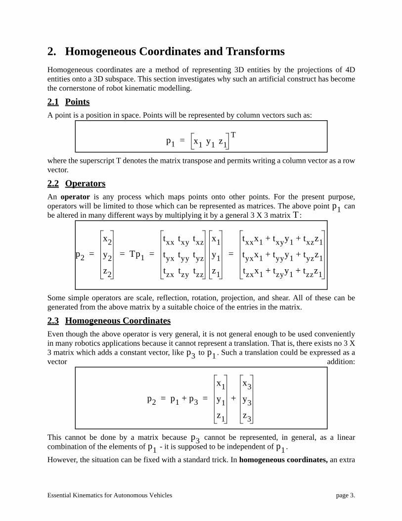
2.1 PointsA point is a position in space. Points will be represented by column vectors such as:

where the superscript T denotes the matrix transpose and permits writing a column vector as a rowvector.

2.2 OperatorsAn operator is any process which maps points onto other points. For the present purpose,operators will be limited to those which can be represented as matrices. The above point canbe altered in many different ways by multiplying it by a general 3 X 3 matrix :

Some simple operators are scale, reflection, rotation, projection, and shear. All of these can begenerated from the above matrix by a suitable choice of the entries in the matrix.

2.3 Homogeneous CoordinatesEven though the above operator is very general, it is not general enough to be used convenientlyin many robotics applications because it cannot represent a translation. That is, there exists no 3 X3 matrix which adds a constant vector, like to . Such a translation could be expressed as avector addition:

This cannot be done by a matrix because cannot be represented, in general, as a linearcombination of the elements of - it is supposed to be independent of .

However, the situation can be fixed with a standard trick. In homogeneous coordinates, an extra

p1 x1 y1 z1T=

p1T

p2

x2y2z2

Tp1

txx txy txztyx tyy tyztzx tzy tzz

x1y1z1

txxx1 txyy1 txzz1+ +

tyxx1 tyyy1 tyzz1+ +

tzxx1 tzyy1 tzzz1+ +

= = = =

p3 p1

p2 p1 p3+

x1y1z1

x3y3z3

+= =

p3p1 p1


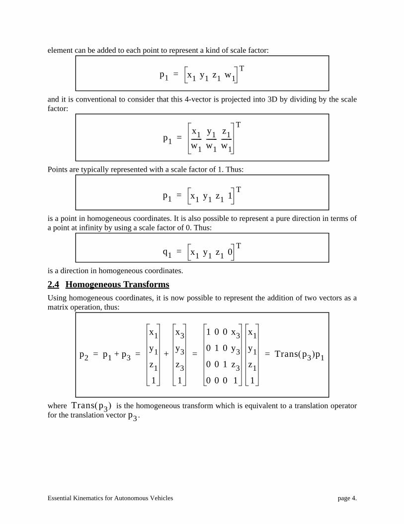
element can be added to each point to represent a kind of scale factor:

and it is conventional to consider that this 4-vector is projected into 3D by dividing by the scalefactor:

Points are typically represented with a scale factor of 1. Thus:

is a point in homogeneous coordinates. It is also possible to represent a pure direction in terms ofa point at infinity by using a scale factor of 0. Thus:

is a direction in homogeneous coordinates.

2.4 Homogeneous TransformsUsing homogeneous coordinates, it is now possible to represent the addition of two vectors as amatrix operation, thus:

where is the homogeneous transform which is equivalent to a translation operatorfor the translation vector .

p1 x1 y1 z1 w1T=

p1x1w1-------

y1w1-------

z1w1-------

T

=

p1 x1 y1 z1 1T=

q1 x1 y1 z1 0T=

p2 p1 p3+

x1y1z11

x3y3z31

+

1 0 0 x30 1 0 y30 0 1 z30 0 0 1

x1y1z11

Trans p3( )p1= = = =

Trans p3( )p3


2.5 Homogeneous Transforms as OperatorsSuppose it is necessary to move a point in some manner and express the result in the samecoordinate system as the original point. This is the notion of an operator. The basic operators aretranslation along and rotation about any of the three axes. The following table gives the fourelementary operators which are sufficient for the purposes of the report, and for almost any realproblems. Operators are identified by an upper case first letter.

It is important to remember the precise semantics of these operators. They take a point expressedin some coordinate system, operate on it, and supply the result expressed in the same coordinatesystem.

One of the most common operators used in robotics is a rotation followed by a translation. Thehomogeneous transform can be used to represent this operator as a single matrix. In general, manykinds of operators can be represented by homogeneous transforms. However, the operatorinterpretation is but one of three possible interpretations of the homogeneous transform.

x

y

z

Trans u v w, ,( )

1 0 0 u0 1 0 v0 0 1 w0 0 0 1

=

z

x

y

φ

Roty φ( )

cφ 0 sφ 00 1 0 0s– φ 0 cφ 00 0 0 1

=

y

z

x

θRotx θ( )

1 0 0 00 cθ sθ– 00 sθ cθ 00 0 0 1

=

x

y

z

ψRotz ψ( )

cψ s– ψ 0 0sψ cψ 0 00 0 1 00 0 0 1

=


2.6 Example - Operating on a PointThe homogeneous coordinates of the origin are clearly:

As an example of applying operators to a point, the following figure indicates the result oftranslating the origin along the y axis by ‘v’ units and then rotating the resulting point by 90°around the x axis.

Notice that the operators are written in right to left order because this is the order in which they areapplied to the original column vector representing the origin. The order is important because matrixmultiplication is not commutative. Also notice that the initial point, intermediate point, and finalresult are all expressed in terms of the axes of the original coordinate system. Operators have fixedaxis semantics.

2.7 Homogeneous Transforms as Coordinate FramesRecall that homogeneous coordinates can be used to represent directions as well as points. This isdone by using a zero scale factor. The unit vectors of a cartesian coordinate system can beconsidered to be directions. The x, y, and z unit vectors can be written as:

Therefore, these three columns can be grouped together with the homogeneous coordinates of the

o

o 0 0 0 1T=

x

y

z

p Rotx π 2⁄( )Trans 0 v 0, ,( )o=

p

1 0 0 00 0 1– 00 1 0 00 0 0 1

1 0 0 00 1 0 v0 0 1 00 0 0 1

0001

1 0 0 00 0 1– 00 1 0 00 0 0 1

0v01

00v1

= = =

o' 0 v 0 1T=

p 0 0 v 1T=

v

i 1 0 0 0T= j 0 1 0 0

T= k 0 0 1 0T=


origin to form an identity matrix:

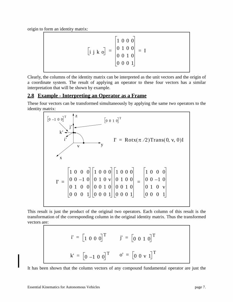
Clearly, the columns of the identity matrix can be interpreted as the unit vectors and the origin ofa coordinate system. The result of applying an operator to these four vectors has a similarinterpretation that will be shown by example.

2.8 Example - Interpreting an Operator as a FrameThese four vectors can be transformed simultaneously by applying the same two operators to theidentity matrix:

This result is just the product of the original two operators. Each column of this result is thetransformation of the corresponding column in the original identity matrix. Thus the transformedvectors are:

It has been shown that the column vectors of any compound fundamental operator are just the

i j k o

1 0 0 00 1 0 00 0 1 00 0 0 1

I= =

I' Rotx π 2⁄( )Trans 0 v 0, ,( )I=

I'

1 0 0 00 0 1– 00 1 0 00 0 0 1

1 0 0 00 1 0 v0 0 1 00 0 0 1

1 0 0 00 1 0 00 0 1 00 0 0 1

1 0 0 00 0 1– 00 1 0 v0 0 0 1

= =

x

y

j’

v

k’i’

0 1– 0 0T

0 0 1 0Tz

i' 1 0 0 0T= j' 0 0 1 0

T=

k' 0 1– 0 0T= o' 0 0 v 1

T=


homogeneous coordinates of the transformed unit vectors and the origin. This is because theoperators apply to any vectors - including the origin and the unit vectors. The result can bevisualized by drawing the new transformed axes at the new position.

2.9 The Coordinate FrameSo far in the discussion, there are two complementary interpretations of exactly the same 4 X 4matrix. It can be an operator which moves points and vectors around, or it can be a representationof a cartesian coordinate system positioned somewhere in space relative to another one. Cartesiancoordinate systems positioned in space are a central concept in 3D kinematics. They encode botha position and an attitude. With an encoded position and attitude available, it becomes possible totalk about the state of motion of the origin in terms of translation and orientation and all of theirassociated time derivatives. Therefore, this entity embodies the properties of a frame of reference.

With a set of three orthogonal unit vectors, it is possible to represent an arbitrary vector quantity interms of its projections onto these axes. Therefore, this entity also embodies the properties of acartesian coordinate system. This moving set of unit vectors is often called a coordinate frame orsimply a frame. Often, imaginary frames are embedded in the links of a mechanism in order tokeep track of its configuration. These embedded frames are central to the study of manipulators,legs and other mechanisms.

2.10 Homogeneous Transforms as Coordinate TransformsThere is a third interpretation of a homogeneous transform. It was shown that they move points andmove and orient frames and that they directly represent frames. However, if they move frames, onecan think about the original frame and the transformed frame as two different frames and then askabout the relationship between the coordinates of any point in each frame. Let the original framebe called ‘a’ and the transformed one be called ‘b’.

Let a general point be expressed in the coordinates of frame ‘b’. This will be represented by asuperscript b. Its coordinates in this frame are:

Alternately, it can be written as a true physical vector thus:

This vector can be expressed in the coordinates of frame ‘a’ by expressing the unit vectors of frame‘b’ in the coordinates of frame ‘a’ and adding the position of the origin, thus:

p

pbxb yb zb 1=

pb xbib ybjb zbkb+ +=

pa xbi' ybj' zbk' o'+ + +=


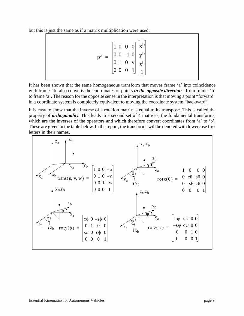
but this is just the same as if a matrix multiplication were used:

It has been shown that the same homogeneous transform that moves frame ‘a’ into coincidencewith frame ‘b’ also converts the coordinates of points in the opposite direction - from frame ‘b’to frame ‘a’. The reason for the opposite sense in the interpretation is that moving a point “forward”in a coordinate system is completely equivalent to moving the coordinate system “backward”.

It is easy to show that the inverse of a rotation matrix is equal to its transpose. This is called theproperty of orthogonality. This leads to a second set of 4 matrices, the fundamental transforms,which are the inverses of the operators and which therefore convert coordinates from ‘a’ to ‘b’.These are given in the table below. In the report, the transforms will be denoted with lowercase firstletters in their names.

pa

1 0 0 00 0 1– 00 1 0 v0 0 0 1

xb

yb

zb

1

=

xa

ya

za

trans u v w, ,( )

1 0 0 u–0 1 0 v–0 0 1 w–0 0 0 1

=

roty φ( )

cφ 0 s– φ 00 1 0 0sφ 0 cφ 00 0 0 1

=

ya

za

xa,xb

θrotx θ( )

1 0 0 00 cθ sθ 00 s– θ cθ 00 0 0 1

=

rotz ψ( )

cψ sψ 0 0s– ψ cψ 0 00 0 1 00 0 0 1

=

xb

yb

zb

yb

θ

zb

za

xa

ya,yb

φ

zb

φ

xb

xa

ya

za,zb

ψ

xb

ψ

yb


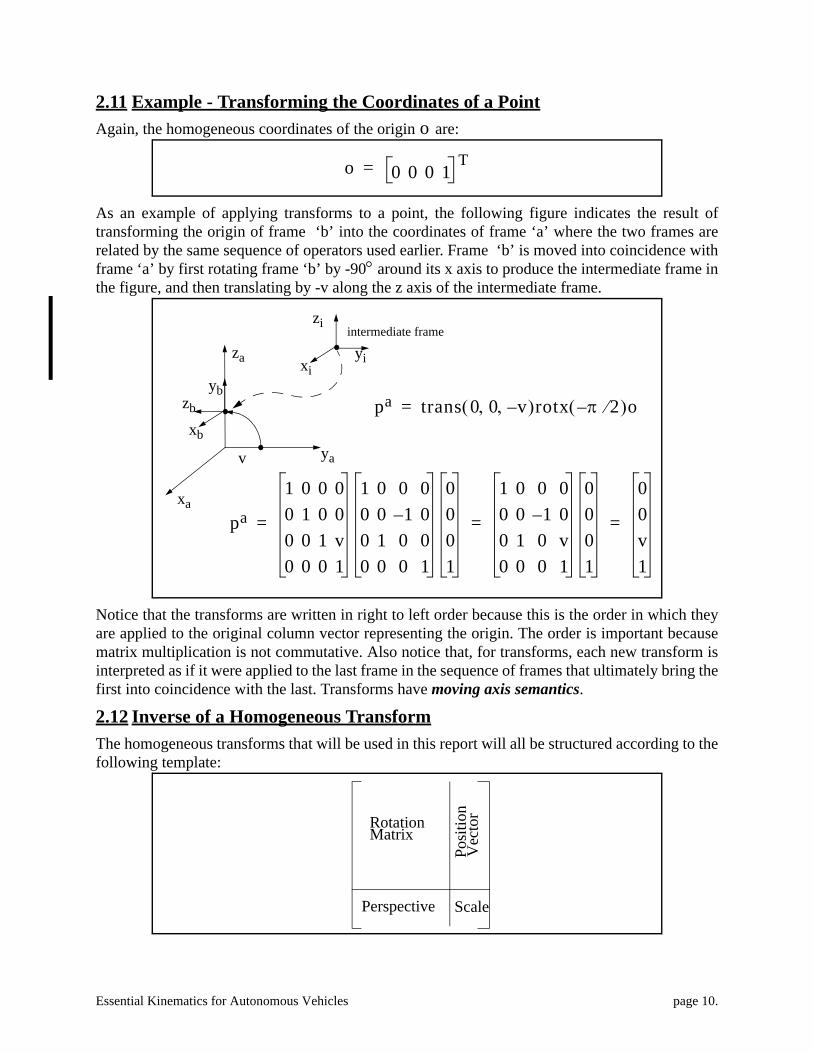
2.11 Example - Transforming the Coordinates of a PointAgain, the homogeneous coordinates of the origin are:

As an example of applying transforms to a point, the following figure indicates the result oftransforming the origin of frame ‘b’ into the coordinates of frame ‘a’ where the two frames arerelated by the same sequence of operators used earlier. Frame ‘b’ is moved into coincidence withframe ‘a’ by first rotating frame ‘b’ by -90° around its x axis to produce the intermediate frame inthe figure, and then translating by -v along the z axis of the intermediate frame.

Notice that the transforms are written in right to left order because this is the order in which theyare applied to the original column vector representing the origin. The order is important becausematrix multiplication is not commutative. Also notice that, for transforms, each new transform isinterpreted as if it were applied to the last frame in the sequence of frames that ultimately bring thefirst into coincidence with the last. Transforms have moving axis semantics.

2.12 Inverse of a Homogeneous TransformThe homogeneous transforms that will be used in this report will all be structured according to thefollowing template:

o

o 0 0 0 1T=

pa trans 0 0 v–, ,( )rotx π– 2⁄( )o=

pa

1 0 0 00 1 0 00 0 1 v0 0 0 1

1 0 0 00 0 1– 00 1 0 00 0 0 1

0001

1 0 0 00 0 1– 00 1 0 v0 0 0 1

0001

00v1

= = =xa

yav

za

xb

ybzb

xiyi

ziintermediate frame

Perspective Scale

RotationMatrix

Posi

tion

Vec

tor


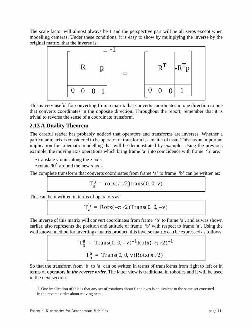
The scale factor will almost always be 1 and the perspective part will be all zeros except whenmodelling cameras. Under these conditions, it is easy to show by multiplying the inverse by theoriginal matrix, that the inverse is:

This is very useful for converting from a matrix that converts coordinates in one direction to onethat converts coordinates in the opposite direction. Throughout the report, remember that it istrivial to reverse the sense of a coordinate transform.

2.13 A Duality TheoremThe careful reader has probably noticed that operators and transforms are inverses. Whether aparticular matrix is considered to be operator or transform is a matter of taste. This has an importantimplication for kinematic modelling that will be demonstrated by example. Using the previousexample, the moving axis operations which bring frame ‘a’ into coincidence with frame ‘b’ are:

• translate v units along the z axis• rotate 90° around the new x axis

The complete transform that converts coordinates from frame ‘a’ to frame ‘b’ can be written as:

This can be rewritten in terms of operators as:

The inverse of this matrix will convert coordinates from frame ‘b’ to frame ‘a’, and as was shownearlier, also represents the position and attitude of frame ‘b’ with respect to frame ‘a’. Using thewell known method for inverting a matrix product, this inverse matrix can be expressed as follows:

So that the transform from ‘b’ to ‘a’ can be written in terms of transforms from right to left or interms of operators in the reverse order. The latter view is traditional in robotics and it will be usedin the next section.1

1. One implication of this is that any set of rotations about fixed axes is equivalent to the same set executed in the reverse order about moving axes.

0

R

0 0 1

p

0

RT

0 0 1

-RTp=

-1

Tab rotx π 2⁄( )trans 0 0 v, ,( )=

Tab Rotx π– 2⁄( )Trans 0 0 v–, ,( )=

Tba Trans 0 0 v–, ,( ) 1– Rotx π– 2⁄( ) 1–=

Tba Trans 0 0 v, ,( )Rotx π 2⁄( )=


3. Forward KinematicsForward kinematics is the relatively straightforward process of chaining homogeneous transformstogether in order to represent the articulations of a mechanism or simply to represent the fixedtransformation between two frames. In this process, the joint variables are given, and the problemis to find the transform.

3.1 Nonlinear MappingIt is clear that it is possible to transform coordinates between coordinate systems which are fixedin position and attitude with respect to each other. It is also possible to perform elementaryoperations with homogeneous transforms. Ultimately, this is possible because such operations arelinear. That is, the result is always a weighted sum of the original point or vector.

Most mechanisms, however, are not linear. They are composed of one or more rotary degrees offreedom. It turns out that the homogeneous transform can still be used to model such complexdevices if they are viewed in a different way. In the study of mechanisms, the parameters of therotations and translations between the frames are considered to be variables. In this sense, theproblem is one of understanding the variation in a homogeneous transform when it is consideredto be a function of one or more variables.

In the study of mechanisms, the real world space in which a mechanism moves is often called taskspace, and points and vectors are normally expressed in terms of cartesian coordinates. However,the mechanism articulations are most easily expressed in terms of angles and displacements alongaxes. This space is called configuration space. So far, we have studied linear transformationswithin task space. This section and the following sections will consider the more difficult problemof expressing the relationship between task space and configuration space. This problem is one ofmultidimensional nonlinear mapping.

3.2 Mechanism ModelsIt is natural to think about the operation of a mechanism in a moving axes sense - because mostmechanisms are built that way. That is, the position and orientation of any link in a kinematic chainis dependent on all other joints that come before it in the sequence.

Conventionally, one thinks in terms of moving axis operations applied to frames embedded in themechanism which move the first frame sequentially into coincidence with all of the others in themechanism. Then, a sequence of operators is written to represent the mechanism kinematics. Theconventional rules for modelling a sequence of connected joints are as follows:

• assign embedded frames to the links in sequence such that the operations which move eachframe into coincidence with the next are a function of the appropriate joint variable

• write the operator matrices which correspond to these operations in left to right order This process will generate the matrix that represents the position of the last embedded frame withrespect to the first, or equivalently, which converts the coordinates of a point from the last to thefirst. This matrix will be called the mechanism model.


3.3 Modelling a MechanismIn 1955, J. Denavit and R. S. Hartenberg [3] first proposed the use of homogeneous transforms torepresent the articulations of a mechanism, and this form of model has been used almostuniversally since. A mechanism is considered to be any collection of joints, either linear or rotary,joined together by links. The total number of movable joints is called the number of degrees offreedom.

3.4 Denavit Hartenberg Convention for MechanismsIt is conventional in many aspects of robotics to use a special product of four fundamental operatorsas a basic conceptual unit. The resulting single matrix can represent the most general spatialrelationship between two frames. This convention with a small number of associated rules forassignment of embedded frames has come to be called the Denavit Hartenberg (DH) convention.

For two frames positioned in space, the directions of, say, the z axes of two frames define two linesin 3D space. For nonparallel axes, there is a well defined measure of the distance between themgiven by the length of their mutual perpendicular. Let the first frame be called frame i-1 and thesecond frame i. The first can be moved into coincidence with the second by a sequence of 4operations:

• rotate around the xi-1 axis by an angle θi• translate along the xi-1 axis by a distance ui• rotate around the new z axis by an angle ψi• translate along the new z axis by a distance wi

Joints

Links


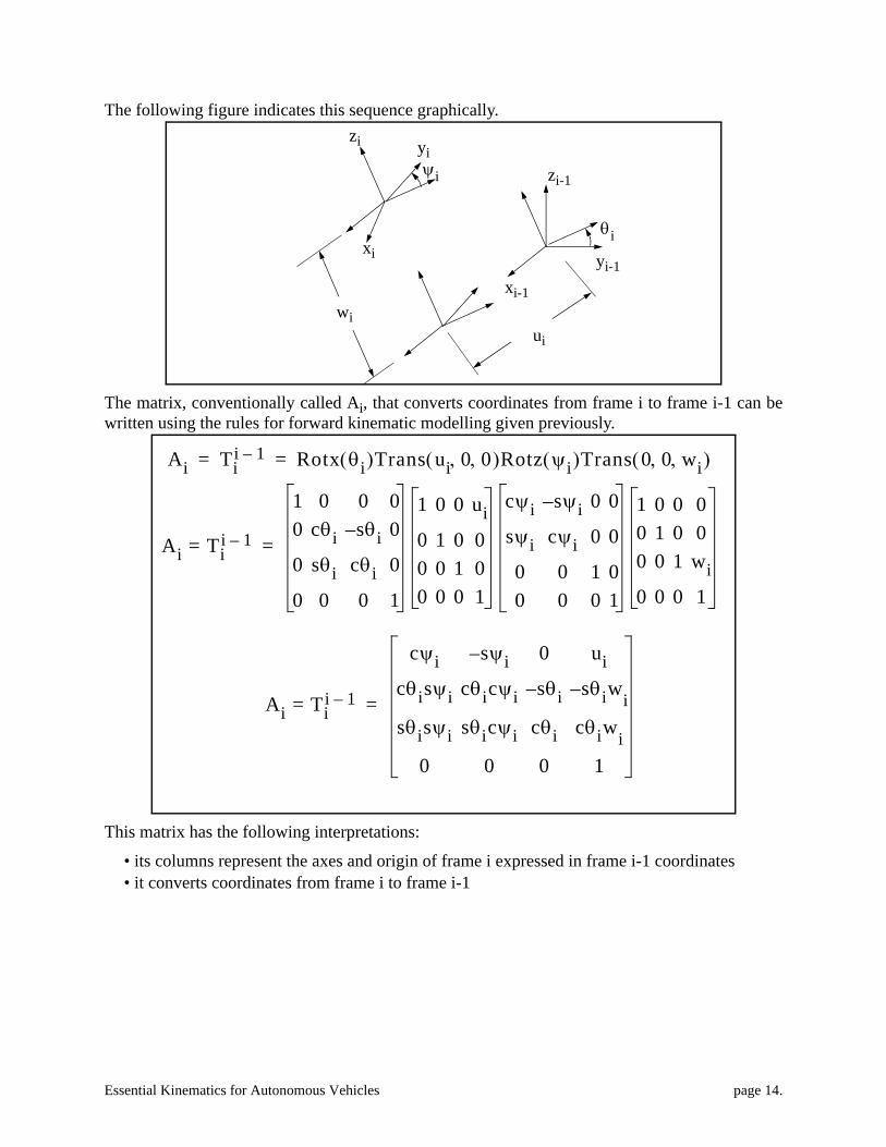
The following figure indicates this sequence graphically.

The matrix, conventionally called Ai, that converts coordinates from frame i to frame i-1 can bewritten using the rules for forward kinematic modelling given previously.

This matrix has the following interpretations:

• its columns represent the axes and origin of frame i expressed in frame i-1 coordinates• it converts coordinates from frame i to frame i-1

xi-1

yi-1

zi-1

θi

ψi

zi yi

xi

ui

wi

Ai Tii 1– Rotx θi( )Trans ui 0 0, ,( )Rotz ψi( )Trans 0 0 wi, ,( )= =

Ai Tii 1–=

1 0 0 00 cθi s– θi 0

0 sθi cθi 0

0 0 0 1

1 0 0 ui0 1 0 00 0 1 00 0 0 1

cψi s– ψi 0 0

sψi cψi 0 0

0 0 1 00 0 0 1

1 0 0 00 1 0 00 0 1 wi0 0 0 1

=

Ai Tii 1–=

cψi s– ψi 0 uicθisψi cθicψi s– θi s– θiwisθisψi sθicψi cθi cθiwi

0 0 0 1

=


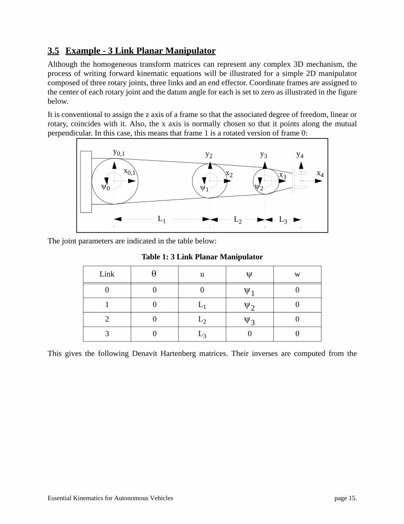
3.5 Example - 3 Link Planar ManipulatorAlthough the homogeneous transform matrices can represent any complex 3D mechanism, theprocess of writing forward kinematic equations will be illustrated for a simple 2D manipulatorcomposed of three rotary joints, three links and an end effector. Coordinate frames are assigned tothe center of each rotary joint and the datum angle for each is set to zero as illustrated in the figurebelow.

It is conventional to assign the z axis of a frame so that the associated degree of freedom, linear orrotary, coincides with it. Also, the x axis is normally chosen so that it points along the mutualperpendicular. In this case, this means that frame 1 is a rotated version of frame 0:

The joint parameters are indicated in the table below:

This gives the following Denavit Hartenberg matrices. Their inverses are computed from the

Table 1: 3 Link Planar Manipulator

Link u w

0 0 0 0

1 0 L1 0

2 0 L2 0

3 0 L3 0 0

x0,1

y0,1

x2

y2

x3

y3

x4

y4

L1 L2 L3

ψ1ψ0 ψ2

θ ψ

ψ1ψ2ψ3


inverse formula because they will be useful later:

The position and orientation of the end effector with respect to the base is given by:

A1

c1 s1– 0 0

s1 c1 0 0

0 0 1 00 0 0 1

=

A2

c2 s2– 0 L1s2 c2 0 0

0 0 1 00 0 0 1

=

A3

c3 s3– 0 L2s3 c3 0 0

0 0 1 00 0 0 1

=

A4

1 0 0 L30 1 0 00 0 1 00 0 0 1

=

A11–

c1 s1 0 0

s1– c1 0 0

0 0 1 00 0 0 1

=

A21–

c2 s2 0 c2L1–

s2– c2 0 s2L10 0 1 00 0 0 1

=

A31–

c3 s3 0 c– 3L2s3– c3 0 s3L20 0 1 00 0 0 1

=

A41–

1 0 0 L– 30 1 0 00 0 1 00 0 0 1

=


T40 T1

0T21T3

2T43 A1A2A3A4= =

T40

c1 s1– 0 0

s1 c1 0 0

0 0 1 00 0 0 1

c2 s2– 0 L1s2 c2 0 0

0 0 1 00 0 0 1

c3 s3– 0 L2s3 c3 0 0

0 0 1 00 0 0 1

1 0 0 L30 1 0 00 0 1 00 0 0 1

=

T40

c123 s123– 0 c123L3 c12L2 c1L1+ +( )

s123 c123 0 s123L3 s12L2 s1L1+ +( )

0 0 1 00 0 0 1

=


4. Inverse KinematicsInverse kinematics is the problem of finding the joint parameters given only the numerical valuesof the homogeneous transforms which model the mechanism. In practice, this is useful because itsolves the problem of where to drive the joints in order to get the hand of an arm or the foot of aleg in the right place, at the right orientation.

Proficiency with inverse kinematics requires a degree of skill and practice and there are fewgeneral guidelines that can be given. This section will discuss this difficult problem and continuewith the simple example.

4.1 Existence and UniquenessThe inverse kinematic problem is considerably more difficult than the forward one because itinvolves the solution of nonlinear equations. In general, there is no guarantee that nonlinearequations have a solution, and if they do, it may not be unique. It has been shown theoretically byPieper [13], that a six degree of freedom manipulator for which the last three joints intersect at apoint is always solvable. Most manipulators are constructed in this way, so most are solvable.

Any real mechanism has a finite reach, so it can only achieve positions in a region of space knownas the workspace. Unless the initial transform to be solved is in the workspace, the inversekinematic problem will have no solution. This manifests itself, for example, as inverse sines andcosines of arguments greater than one. Further, mechanisms with many rotary joints will often havemore than one solution, which will exhibit various forms of symmetry. The latter case is known asredundancy.

4.2 TechniqueThis problem would be very difficult to solve without the discipline afforded by the use ofhomogeneous transforms. Using the DH convention, a mechanism can be “solved” more or lessone joint at a time by a process of rewriting the forward kinematics equations in several differentways.

Any DH matrix has only six degrees of freedom. The rotation matrix part is constrained to beorthonormal. That is, the rows or columns must be of unit length and mutually perpendicular. Thebottom row is constrained to contain zeros and ones. The position vector contains threeindependent values.

The inverse kinematic problem is solved by rewriting the forward transform in many differentways in an attempt to isolate unknowns. Although there are only 6 independent relationships, theycan be rewritten in many different ways.

Using a 3 degree of freedom mechanism for example, the forward kinematics can be written in all


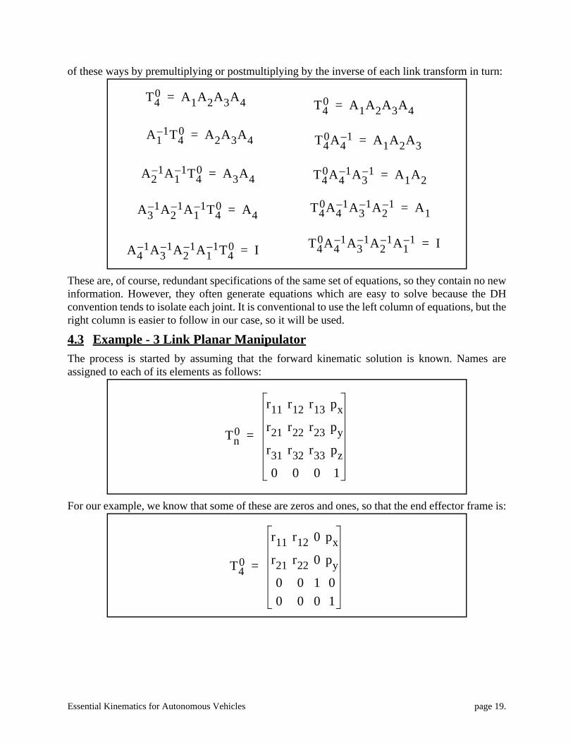
of these ways by premultiplying or postmultiplying by the inverse of each link transform in turn:

These are, of course, redundant specifications of the same set of equations, so they contain no newinformation. However, they often generate equations which are easy to solve because the DHconvention tends to isolate each joint. It is conventional to use the left column of equations, but theright column is easier to follow in our case, so it will be used.

4.3 Example - 3 Link Planar ManipulatorThe process is started by assuming that the forward kinematic solution is known. Names areassigned to each of its elements as follows:

For our example, we know that some of these are zeros and ones, so that the end effector frame is:

T40 A1A2A3A4=

A11– T4

0 A2A3A4=

A21– A1

1– T40 A3A4=

A31– A2

1– A11– T4

0 A4=

A41– A3

1– A21– A1

1– T40 I=

T40 A1A2A3A4=

T40A4

1– A1A2A3=

T40A4

1– A31– A1A2=

T40A4

1– A31– A2

1– A1=

T40A4

1– A31– A2

1– A11– I=

Tn0

r11 r12 r13 pxr21 r22 r23 pyr31 r32 r33 pz0 0 0 1

=

T40

r11 r12 0 pxr21 r22 0 py0 0 1 00 0 0 1

=


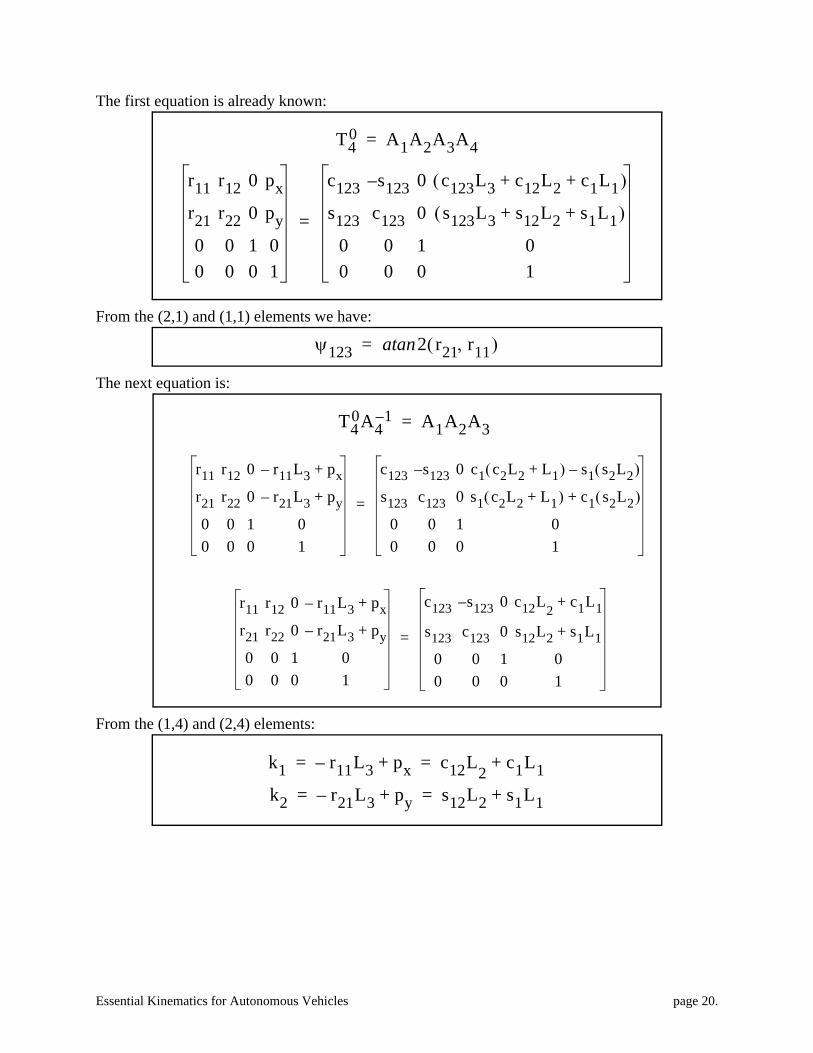
The first equation is already known:

From the (2,1) and (1,1) elements we have:

The next equation is:

From the (1,4) and (2,4) elements:

r11 r12 0 pxr21 r22 0 py0 0 1 00 0 0 1

c123 s123– 0 c123L3 c12L2 c1L1+ +( )

s123 c123 0 s123L3 s12L2 s1L1+ +( )

0 0 1 00 0 0 1

=

T40 A1A2A3A4=

ψ123 2 r21 r11,( )atan=

T40A4

1– A1A2A3=

r11 r12 0 r11L3– px+

r21 r22 0 r21L3– py+

0 0 1 00 0 0 1

c123 s123– 0 c12L2 c1L1+

s123 c123 0 s12L2 s1L1+

0 0 1 00 0 0 1

=

r11 r12 0 r11L3– px+

r21 r22 0 r21L3– py+

0 0 1 00 0 0 1

c123 s123– 0 c1 c2L2 L1+( ) s1 s2L2( )–

s123 c123 0 s1 c2L2 L1+( ) c1 s2L2( )+

0 0 1 00 0 0 1

=

k1 r11L3– px+ c12L2 c1L1+= =

k2 r21L3– py+ s12L2 s1L1+= =


These can be squared and added to yield:

And this gives the angle as:

The result implies that there are two solutions for this angle which are symmetric about zero. Thesecorrespond to the elbow up and elbow down configurations. Now, before the expressions werereduced to include a sum of angles, they were:

With now known, these can be written as:

This is one of the standard forms that recur in inverse kinematics problems for which the solutionis:

Finally, the last angle is:

k12 k2

2+ L22 L1

2 2L2L1 c1c12 s1s12+( )+ +=

k12 k2

2+ L22 L1

2 2L2L1c2+ +=

ψ2

ψ2k1

2 k22+( ) L2

2 L12+( )–

2L2L1------------------------------------------------------acos=

k1 r11L3– px+ c1 c2L2 L1+( ) s1 s2L2( )–= =

k2 r21L3– py+ s1 c2L2 L1+( ) c1 s2L2( )+= =

ψ2

c1k3 s1k4– k1=s1k3 c1k4+ k2=

ψ1 2atan k2k3 k1k4–( ) k1k3 k2k4+( ),[ ]=

ψ3 ψ123 ψ2 ψ1––=


4.4 Standard FormsThere are a few forms of trigonometric equations that recur is most mechanisms. The following setof solutions is sufficient for most applications. One of the most difficult forms, solved by squareand add, was presented in the example. In the following, the letters a, b, and c represent arbitraryknown expressions.

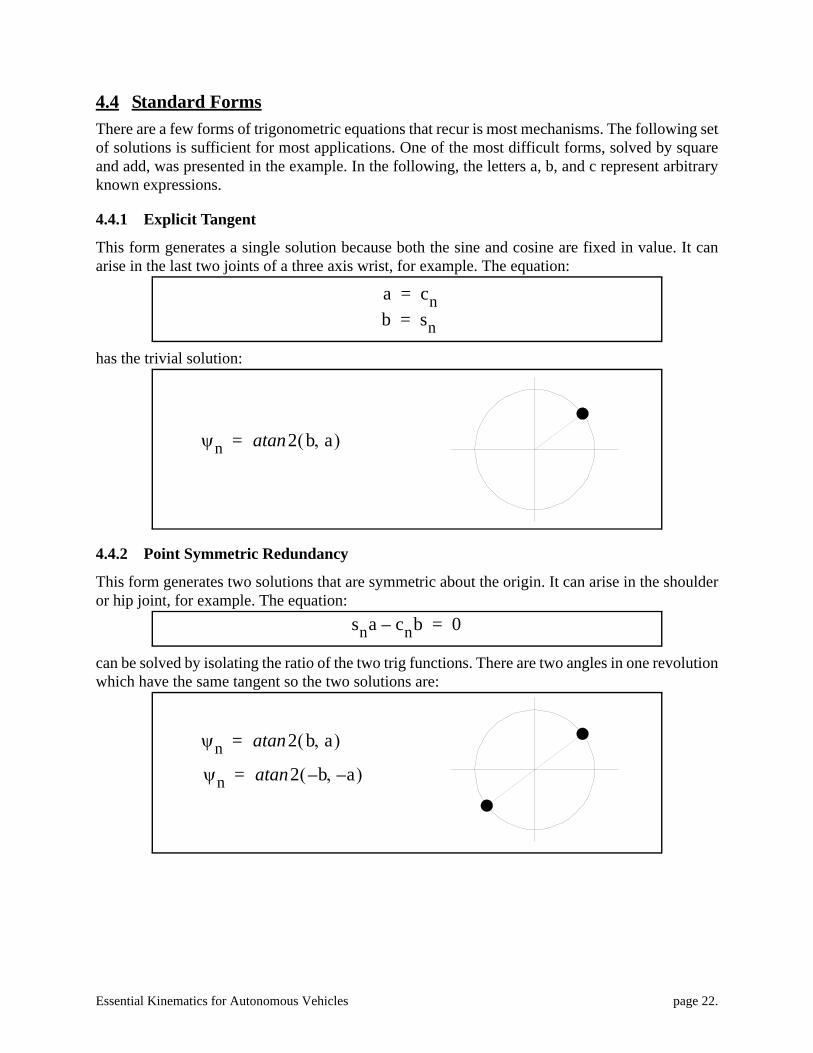
4.4.1 Explicit Tangent

This form generates a single solution because both the sine and cosine are fixed in value. It canarise in the last two joints of a three axis wrist, for example. The equation:

has the trivial solution:

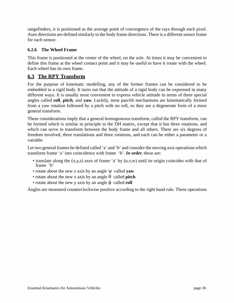
4.4.2 Point Symmetric Redundancy

This form generates two solutions that are symmetric about the origin. It can arise in the shoulderor hip joint, for example. The equation:

can be solved by isolating the ratio of the two trig functions. There are two angles in one revolutionwhich have the same tangent so the two solutions are:

a cn=b sn=

ψn 2 b a,( )atan=

sna cnb– 0=

ψn 2 b a,( )atan=

ψn 2 b– a–,( )atan=


4.4.3 Line Symmetric Redundancy

This form generates two solutions that are symmetric about an axis because the sine or cosine ofthe deviation from the axis must be constant. The sine case will be illustrated. It can arise in theshoulder or hip joint, or in an elbow or knee joint, for example. The equation:

can be solved by the trig substitution:

where:

This gives:

So the cosine is:

This gives the result:

sna cnb– c=

a r θ( )cos= b r θ( )sin=

r sqrt a2 b2+( )±= θ 2 b a,( )atan=

sncθ cnsθ– c r⁄=

s θ ψn–( ) c r⁄=

c θ ψn–( ) sqrt 1 c r⁄( )2–( )±=

ψn 2 b a,( ) 2 c sqrt r2 c2–( )±,[ ]atan–atan= ba


5. Differential KinematicsDifferential kinematics is the study of the derivatives of kinematic models. These derivatives arecalled Jacobians and they have many uses ranging from:

• resolved rate control• sensitivity analysis• uncertainty propagation• static force transformation

5.1 Derivatives of Fundamental OperatorsThe derivatives of the fundamental operators with respect to their own parameters will beimportant. They can be used to compute derivatives of very complex expressions by using thechain rule of differentiation. For reference, they are quoted below:

Similar expressions can be generated for the fundamental transforms.

5.2 The Mechanism JacobianIf a sequence of joints can be represented by the product of a series of homogeneous transforms, itis natural to ask about the effect of a differential change in joint variables on the position andorientation of the end of the mechanism. A frame matrix represents orientation indirectly in termsof three unit vectors, so an extra set of equations is required to extract three angles from the rotationmatrix in order to represent orientation. In terms of position, however, the last column of themechanism model gives the position of the end effector with respect to the base.

In general, let a mechanism have variables represented by the vector , and let the position andorientation, or pose, of the end of the mechanism be given by the vector . Then, the end effector

u∂∂ Trans u v w, ,( )

1 0 0 10 1 0 00 0 1 00 0 0 1

=

v∂∂ Trans u v w, ,( )

1 0 0 00 1 0 10 0 1 00 0 0 1

=

w∂∂ Trans u v w, ,( )

1 0 0 00 1 0 00 0 1 10 0 0 1

=

θ∂∂ Rotx θ( )

1 0 0 00 s– θ c– θ 00 cθ s– θ 00 0 0 1

=

φ∂∂ Roty φ( )

s– φ 0 cφ 00 1 0 0c– φ 0 s– φ 00 0 0 1

=

ψ∂∂ Rotz ψ( )

s– ψ c– ψ 0 0cψ s– ψ 0 00 0 1 00 0 0 1

=

qx


position is given by:

where the nonlinear multidimensional function comes from the mechanism model. The Jacobianmatrix is a multidimensional derivative defined as:

The differential mapping from small changes in to the corresponding small changes in is:

The Jacobian also gives velocity relationships via the chain rule of differentiation as follows:

which maps joint rates onto end effector velocity. Note that the Jacobian is nonlinear in the jointvariables, but linear in the joint rates. This implies that reducing the joint rates by half reduces theend velocity by exactly half and preserves the direction.

5.3 SingularityRedundancy takes the form of singularity of the Jacobian matrix in the differential kinematicsolution. A mechanism can lose one or more degrees of freedom:

• at points where two different inverse kinematic solutions converge• when joint axes become aligned or parallel• when the boundaries of the workspace are reached

Singularity implies that the Jacobian loses rank and is not invertible. At the same time, the inversekinematic solution tends to fail because axes become aligned, and infinite rates can be generatedby rate control laws.

x F q( )=

F

Jq∂∂ x

q∂∂ F q( )( )

qj∂

∂xiq1∂

∂x1 …qn∂

∂xn

… … …

q1∂

∂xn …qn∂

∂xn

= = = =

q x

dx Jdq=

tdd x

q∂∂ x⎝ ⎠

⎛ ⎞td

d q⎝ ⎠⎛ ⎞=


5.4 Example - 3 Link Planar ManipulatorFor the example manipulator, the last column of the manipulator model gives the following twoequations:

which can be differentiated with respect to , , and in order to determine the velocity ofthe end effector as the joints move. The solution is:

which can be written as:

5.5 Jacobian DeterminantIt is known from the implicit function theorem of calculus that the ratio of differential volumesbetween the domain and range of a multidimensional mapping is given by the Jacobiandeterminant. This quantity has applications to a technique of navigation and ranging calledtriangulation.

Thus the product of the differentials forms a volume in both configuration space and in task space.The relationship between them is:

x c123L3 c12L2 c1L1+ +( )=

y s123L3 s12L2 s1L1+ +( )=

ψ1 ψ2 ψ3

x· s123ψ·

123L3 s12ψ·

12L2 s1ψ·

1L1+ +( )–=

y· c123ψ·

123L3 c12ψ·

12L2 c1ψ·

1L1+ +( )=

x·

y·s123L3– s12L2– s1L1–( ) s123L3– s12L2–( ) s123L3–

c123L3 c12L2 c1L1+ +( ) c123L3 c12L2+( ) c123L3

ψ· 1

ψ· 2

ψ· 3

=

dx1dx2…dxn( ) J dq1dq2…dqm( )=


5.6 Jacobian TensorAt times it is convenient to compute the derivative of a transform matrix with respect to a vectorof variables. In this case, the result is the derivative of a matrix with respect to a vector. Forexample:

This is a three dimensional cube of numbers which can loosely be called a tensor. The mechanismmodel itself is a matrix function of a vector.

For example, if:

Then there are three slices of the tensor, each a matrix, given by:

q∂∂ T q( )[ ] qk∂

∂Tij=

T q( ) A1 q1( )A2 q2( )A3 q3( )=

q1∂∂T

q1∂

∂A1A2A3=

q2∂∂T A1 q2∂

∂A2A3=

q3∂∂T A1A2 q3∂

∂A3=


6. Vehicle KinematicsSome aspects of the kinematics of moving vehicles are simpler than that of mechanisms, others aremore difficult. This section presents an abbreviated discussion of the kinematic transformsnecessary for control of a vehicle in 3D.

6.1 Axis ConventionsThere are at least two prevailing conventions for the assignment of axes for the coordinate systemsof vehicles. In aerospace vehicles, it is conventional to point the z axis downward, and this makesit natural to point the x axis forward and the y axis out the right side of the vehicle. The conventionused here is that the z axis points up, y forward, and x out the right side. This has the advantagethat the projection of 3D information onto the x-y plane is more natural.

It is important to note that the form of rotation matrices depends firstly on the order of theircomponent rotations, and secondly on the linear axis conventions. The convention used herecorresponds to a z-x-y Euler angle sequence. Therefore, it is not advisable to use thehomogeneous transforms developed here until they are verified to be correct for any sensors andactuators that are used.

6.2 Frame AssignmentSeveral coordinate frames are important for moving vehicles. For legged vehicles, the framesembedded in the legs are assigned according to the DH convention and the frames for the rest ofthe system are analogous to those for wheeled vehicles. This section will present a set of framesfor wheeled vehicles that occur in most applications.

These frames are indicated in the figure below:

yb

yb

zb

xb

yn

zn

yn

xn

yh

zh

ys

zs

yh,sxh,s

yw

zw

ywxw

yp

zp

yp

xp


6.2.1 The Navigation Frame

This is the coordinate system in which the vehicle position and attitude is ultimately required.Usually, this frame is taken as locally level (i.e. the z axis is perfectly aligned with the local gravityvector, not the local terrain tangent plane). The z, up, or azimuth axis is aligned with the gravityvector, the y, or north axis is aligned with the geographic pole1, and the x axis points east tocomplete a right-handed system. In some applications, any frame that is fixed on the earth issatisfactory whether or not it is aligned with the earth’s fields. This frame is identified by the lettern.

6.2.2 The Body Frame

The body frame is positioned at the point on the vehicle body which is most convenient and isconsidered to be fixed in attitude with respect to the vehicle body. For Ackerman steer vehicles,the center of rear axle is a natural place for this frame. In some applications, the best estimate ofthe position of the center of gravity is more appropriate. The z axis points up, y forward, and x outthe right side. This frame is identified by the letter b.

6.2.3 The Positioner Frame

This frame is positioned at the point on or near any position estimation system which reports itsown position. If the system generates attitude and attitude rates only, this frame is not requiredbecause the attitude of the device will also be that of the vehicle. For an INS, this is typically thecenter of the IMU and for GPS it is the phase center of the antenna2. Axes directions are definedsimilarly to the body frame directions. There is a different positioner frame for each positioningdevice. This frame is identified by the letter p.

6.2.4 The Sensor Head Frame

Sometimes, environmental perception sensors are mounted on stabilized platforms or on pan/tiltmechanisms. These provide isolation of the sensor attitude from that of the vehicle and/or theability of the system to literally point its “head”. Axes directions are defined similarly to the bodyframe directions. In cases where the rotary axes of the device all intersect at a point, this frame ispositioned at the common point of intersection of these axes. Axes directions are defined similarlyto the body frame directions.

In cases where the environmental perception sensor axes are not aligned with respect to those ofthe vehicle (for example, when the sensor looks downward), or in cases where there is amisalignment which must be accounted for, a rigid sensor head can be defined which tilts the bodyaxes into coincidence with those of the sensor. This frame is identified by the letter h.

6.2.5 The Sensor Frame

This frame is positioned at the center of the environmental perception sensor with axis definitionssimilar to the body frame when the sensor points forward. For video cameras, it is positioned onthe optical axis at the image plane behind the lens. For stereo systems, it is positioned eitherbetween both cameras or is associated with the image plane of one of them. For imaging laser

1. The geographic pole is determined by the earth’s spin axis, not the magnetic field.2. The antenna may be nowhere near the GPS receiver.


rangefinders, it is positioned as the average point of convergence of the rays through each pixel.Axes directions are defined similarly to the body frame directions. There is a different sensor framefor each sensor.

6.2.6 The Wheel Frame

This frame is positioned at the center of the wheel, on the axle. At times it may be convenient todefine this frame at the wheel contact point and it may be useful to have it rotate with the wheel.Each wheel has its own frame.

6.3 The RPY TransformFor the purpose of kinematic modelling, any of the former frames can be considered to beembedded in a rigid body. It turns out that the attitude of a rigid body can be expressed in manydifferent ways. It is usually most convenient to express vehicle attitude in terms of three specialangles called roll, pitch, and yaw. Luckily, most pan/tilt mechanisms are kinematically formedfrom a yaw rotation followed by a pitch with no roll, so they are a degenerate form of a moregeneral transform.

These considerations imply that a general homogeneous transform, called the RPY transform, canbe formed which is similar in principle to the DH matrix, except that it has three rotations, andwhich can serve to transform between the body frame and all others. There are six degrees offreedom involved, three translations and three rotations, and each can be either a parameter or avariable.

Let two general frames be defined called ‘a’ and ‘b’ and consider the moving axis operations whichtransform frame ‘a’ into coincidence with frame ‘b’. In order, these are:

• translate along the (x,y,z) axes of frame ‘a’ by (u,v,w) until its origin coincides with that offrame ‘b’

• rotate about the new z axis by an angle called yaw• rotate about the new x axis by an angle called pitch• rotate about the new y axis by an angle called roll

Angles are measured counterclockwise positive according to the right hand rule. These operations

ψθφ


are indicated below for the case of transforming the navigation frame into the body frame.

The forward kinematic transform that represents this sequence of operations is, according to ourrules for forward kinematics:

This matrix has the following two interpretations1:

• its columns represent the axes and origin of frame ‘b’ expressed in frame ‘a’ coordinates• it converts coordinates from frame ‘b’ to frame ‘a’

The matrix can be considered to be the conversion from a pose to a coordinate frame.

1. This transform applies to the Litton INS on the HMMWV, the Stagget stable platform, and the ROS pan/tilt head.

ya

ya

za

ψ

θ

xa

yb

xb

yb

zab

xa

za

xbzb

φ

Tba Trans u v w, ,( )Rotz ψ( )Rotx θ( )Roty φ( )=

Tba

1 0 0 u0 1 0 v0 0 1 w0 0 0 1

cψ s– ψ 0 0sψ cψ 0 00 0 1 00 0 0 1

1 0 0 00 cθ s– θ 00 sθ cθ 00 0 0 1

cφ 0 sφ 00 1 0 0s– φ 0 cφ 00 0 0 1

=

Tba

cψcφ sψsθsφ–( ) s– ψcθ cψsφ sψsθcφ+( ) usψcφ cψsθsφ+( ) cψcθ sψsφ c– ψsθcφ( ) v

c– θsφ sθ cθcφ w0 0 0 1

=


6.4 Frame Parameters for Wheeled VehiclesUsing the RPY transform, it is now possible to specify the parameters and variables which permitcoordinate transformation from anywhere on a vehicle to anywhere else. This is accomplished byspecifying the six degrees of freedom in a table. In the table, var indicates a variable and fixedindicates a fixed parameter:

6.5 Inverse Kinematics for the RPY TransformThe inverse kinematic solution to the RPY transform has at least two uses:

• it gives the angles to which to drive a sensor head, or a directional antenna given the directioncosines of the goal frame

• it gives the attitude of the vehicle given the body frame axes, which often correspond to thelocal tangent plane to the terrain over which it moves

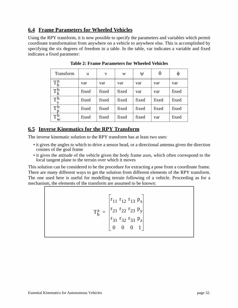
This solution can be considered to be the procedure for extracting a pose from a coordinate frame.There are many different ways to get the solution from different elements of the RPY transform.The one used here is useful for modelling terrain following of a vehicle. Proceeding as for amechanism, the elements of the transform are assumed to be known:

Table 2: Frame Parameters for Wheeled Vehicles

Transform u v w

var var var var var var

fixed fixed fixed var var fixed

fixed fixed fixed fixed fixed fixed

fixed fixed fixed fixed fixed fixed

fixed fixed fixed fixed var fixed

ψ θ φ

Tbn

Thb

Tsh

Tpb

Twb

Tba


=


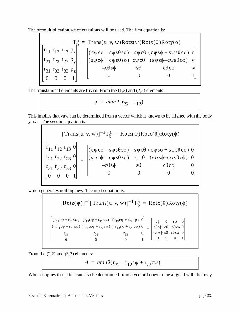
The premultiplication set of equations will be used. The first equation is:

The translational elements are trivial. From the (1,2) and (2,2) elements:

This implies that yaw can be determined from a vector which is known to be aligned with the bodyy axis. The second equation is:

which generates nothing new. The next equation is:


Which implies that pitch can also be determined from a vector known to be aligned with the body

Tba Trans u v w, ,( )Rotz ψ( )Rotx θ( )Roty φ( )=


cψcφ sψsθsφ–( ) s– ψcθ cψsφ sψsθcφ+( ) usψcφ cψsθsφ+( ) cψcθ sψsφ c– ψsθcφ( ) v

c– θsφ sθ cθcφ w0 0 0 1

=

ψ 2 r22 r– 12,( )atan=

Trans u v w, ,( )[ ] 1– Tba Rotz ψ( )Rotx θ( )Roty φ( )=

r11 r12 r13 0

r21 r22 r23 0

r31 r32 r33 0

0 0 0 1

cψcφ sψsθsφ–( ) s– ψcθ cψsφ sψsθcφ+( ) 0sψcφ cψsθsφ+( ) cψcθ sψsφ c– ψsθcφ( ) 0

c– θsφ sθ cθcφ 00 0 0 0

=

Rotz ψ( )[ ] 1– Trans u v w, ,( )[ ] 1– Tba Rotx θ( )Roty φ( )=

r11cψ r21sψ+( ) r12cψ r22sψ+( ) r13cψ r23sψ+( ) 0

r– 11sψ r21cψ+( ) r– 12sψ r22cψ+( ) r– 13sψ r23cψ+( ) 0

r31 r32 r33 0

0 0 0 1

cφ 0 sφ 0sθsφ cθ s– θcφ 0c– θsφ sθ cθcφ 0

0 0 0 1

=

θ 2 r32 r– 12sψ r22cψ+,( )atan=


y axis. A good solution for is available from the (1,1) and (1,3) elements. However, for reasonsof convenience, the solution will be delayed until the next equation. The next equation is:


This implies that roll can be derived from a vector known to be aligned with the body x axis.

6.6 Angular VelocityThe roll, pitch, and yaw angles are, as we have defined them, measured about moving axes.Therefore, they are a sequence of Euler angles, specifically, the z-x-y sequence1. The Euler angledefinition of vehicle attitude has the disadvantage that the roll, pitch, and yaw angles are not thequantities that are actually indicated by strapped down vehicle mounted sensors such as gyros.

The relationship between the rates of the Euler angles and the angular velocity vector is nonlinear.The angles are measured neither about the body axes nor about the navigation frame axes. It isimportant to know the exact relationship between the two because it provides the basis fordetermining vehicle attitude from angular rate measurements.

In order to determine the angular velocity, consider that the total angular velocity is the sum ofthree components, each measured about one of the intermediate axes in the chain of rotations whichbring the navigation frame into coincidence with the body frame. Using the fundamentaltransforms, each of the three rotation rates are transformed into the body frame by the remaining

1. The sequence depends on the convention for assigning the directions of the linear axes.

φ

Rotx θ( )[ ] 1– Rotz ψ( )[ ] 1– Trans u v w, ,( )[ ] 1– Tba Roty φ( )=

r11cψ r21sψ+( ) r12cψ r22sψ+( ) r13cψ r23sψ+( ) 0

cθ r– 11sψ r21cψ+[ ] r31sθ+ cθ r– 12sψ r22cψ+[ ] r32sθ+ cθ r– 13sψ r23cψ+[ ] r33sθ+ 0

sθ– r– 11sψ r21cψ+[ ] r31cθ+ sθ– r– 12sψ r22cψ+[ ] r32cθ+ sθ– r– 13sψ r23cψ+[ ] r33cθ+ 0

0 0 0 1

cφ 0 sφ 00 1 0 0s– φ 0 cφ 00 0 0 1

=

φ 2 sθ r– 11sψ r21cψ+[ ] r31cθ r11cψ r21sψ+( ),–( )atan=


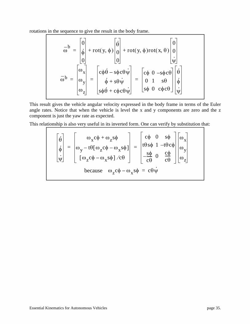
rotations in the sequence to give the result in the body frame.

This result gives the vehicle angular velocity expressed in the body frame in terms of the Eulerangle rates. Notice that when the vehicle is level the x and y components are zero and the zcomponent is just the yaw rate as expected.

This relationship is also very useful in its inverted form. One can verify by substitution that:

ωb

0

φ·

0

rot y φ,( )θ·

00

rot y φ,( )rot x θ,( )00

ψ·+ +=

ωbωxωyωz

cφθ· sφcθψ·–

φ· sθψ·+

sφθ· cφcθψ·+

cφ 0 s– φcθ0 1 sθsφ 0 cφcθ

θ·

φ·

ψ·= = =

θ·

φ·

ψ·

ωxcφ ωzsφ+

ωy tθ ωzcφ ωxsφ–[ ]–

ωzcφ ωxsφ–[ ] cθ⁄

cφ 0 sφtθsφ 1 tθcφ–

sφcθ------– 0 cφ

cθ------

ωxωyωz

= =

ωzcφ ωxsφ– cθψ·=because


7. Sensor KinematicsMany sensors used on robot vehicles are of the imaging variety. For this class of sensors, theprocess of image formation must be modelled. Image coordinates are identified by the letter i.Typically, these transformations are not linear, and hence cannot be modelled by homogeneoustransforms. This section provides the transforms necessary for modelling such sensors. Thesetransforms include projection, reflection, and polar coordinates.

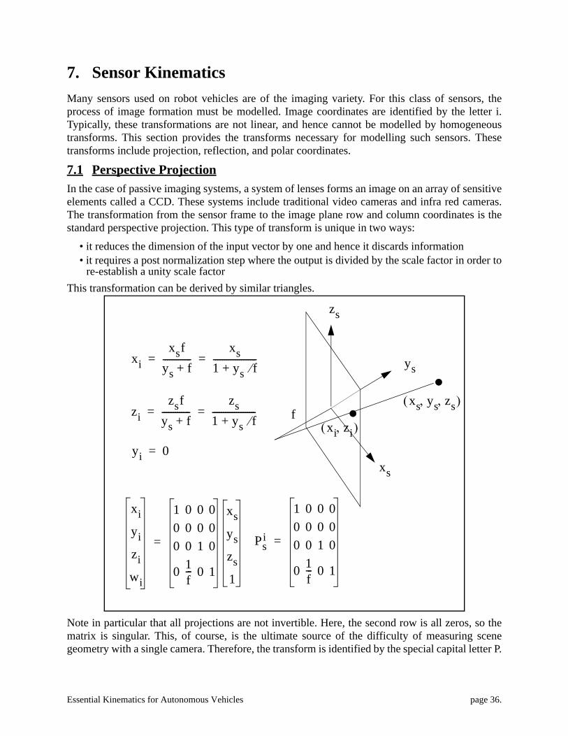
7.1 Perspective ProjectionIn the case of passive imaging systems, a system of lenses forms an image on an array of sensitiveelements called a CCD. These systems include traditional video cameras and infra red cameras.The transformation from the sensor frame to the image plane row and column coordinates is thestandard perspective projection. This type of transform is unique in two ways:

• it reduces the dimension of the input vector by one and hence it discards information• it requires a post normalization step where the output is divided by the scale factor in order to

re-establish a unity scale factorThis transformation can be derived by similar triangles.

Note in particular that all projections are not invertible. Here, the second row is all zeros, so thematrix is singular. This, of course, is the ultimate source of the difficulty of measuring scenegeometry with a single camera. Therefore, the transform is identified by the special capital letter P.

xixsf

ys f+-------------

xs1 ys f⁄+--------------------= =

zizsf

ys f+-------------

zs1 ys f⁄+--------------------= =

yi 0=

ys

xs

zs

xiyiziwi

1 0 0 00 0 0 00 0 1 0

0 1f--- 0 1

xsyszs1

=

fxs ys zs, ,( )

xi zi,( )

Psi

1 0 0 00 0 0 00 0 1 0

0 1f--- 0 1

=


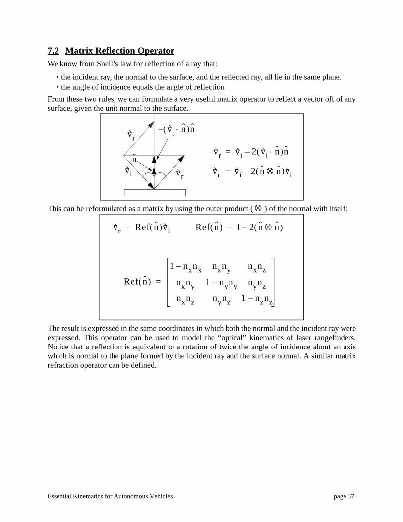
7.2 Matrix Reflection OperatorWe know from Snell’s law for reflection of a ray that:

• the incident ray, the normal to the surface, and the reflected ray, all lie in the same plane. • the angle of incidence equals the angle of reflection

From these two rules, we can formulate a very useful matrix operator to reflect a vector off of anysurface, given the unit normal to the surface.

This can be reformulated as a matrix by using the outer product ( ) of the normal with itself:

The result is expressed in the same coordinates in which both the normal and the incident ray wereexpressed. This operator can be used to model the “optical” kinematics of laser rangefinders.Notice that a reflection is equivalent to a rotation of twice the angle of incidence about an axiswhich is normal to the plane formed by the incident ray and the surface normal. A similar matrixrefraction operator can be defined.

nvi

vrvi n⋅( )n–

vr vi 2 vi n⋅( )n–=

vr vr vi 2 n n⊗( )vi–=

⊗

vr Ref n( )vi= Ref n( ) I 2 n n⊗( )–=

Ref n( )

1 nxnx– nxny nxnznxny 1 nyny– nynznxnz nynz 1 nznz–

=


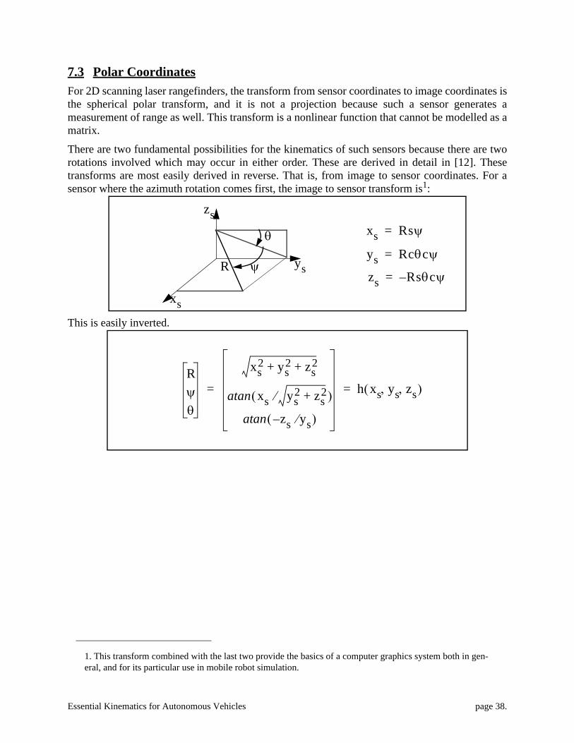
7.3 Polar CoordinatesFor 2D scanning laser rangefinders, the transform from sensor coordinates to image coordinates isthe spherical polar transform, and it is not a projection because such a sensor generates ameasurement of range as well. This transform is a nonlinear function that cannot be modelled as amatrix.

There are two fundamental possibilities for the kinematics of such sensors because there are tworotations involved which may occur in either order. These are derived in detail in [12]. Thesetransforms are most easily derived in reverse. That is, from image to sensor coordinates. For asensor where the azimuth rotation comes first, the image to sensor transform is1:

This is easily inverted.

1. This transform combined with the last two provide the basics of a computer graphics system both in gen-eral, and for its particular use in mobile robot simulation.

xs Rsψ=

ys Rcθcψ=

zs R– sθcψ=

θ

ψ

xs

ys

zs

R

Rψθ

xs2 ys

2 zs2+ +

xs ys2 zs

2+⁄( )atan

z– s ys⁄( )atan

h xs ys zs, ,( )= =


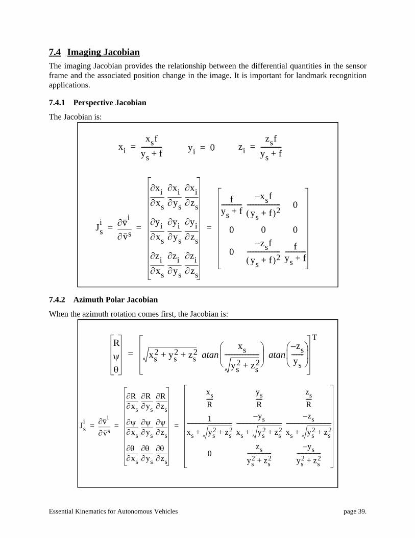
7.4 Imaging JacobianThe imaging Jacobian provides the relationship between the differential quantities in the sensorframe and the associated position change in the image. It is important for landmark recognitionapplications.

7.4.1 Perspective Jacobian

The Jacobian is:

7.4.2 Azimuth Polar Jacobian

When the azimuth rotation comes first, the Jacobian is:

Jsi

vs∂∂vi

xs∂

∂xiys∂

∂xizs∂

∂xi

xs∂

∂yiys∂

∂yizs∂

∂yi

xs∂

∂ziys∂

∂zizs∂

∂zi

fys f+-------------

x– sf

ys f+( )2--------------------- 0

0 0 0

0z– sf

ys f+( )2--------------------- f

ys f+-------------

= = =

xixsf

ys f+-------------= zi

zsfys f+-------------=yi 0=

Rψθ

xs2 ys

2 zs2+ +

xs

ys2 zs

2+----------------------⎝ ⎠⎜ ⎟⎛ ⎞

atanz– s

ys--------⎝ ⎠⎜ ⎟⎛ ⎞

atan

T

=

Jsi

vs∂∂vi

xs∂∂R

ys∂∂R

zs∂∂R

xs∂∂ψ

ys∂∂ψ

zs∂∂ψ

xs∂∂θ

ys∂∂θ

zs∂∂θ

xsR-----

ysR-----

zsR----

1

xs ys2 zs

2++---------------------------------

y– s

xs ys2 zs

2++---------------------------------

z– s

xs ys2 zs

2++---------------------------------

0zs

ys2 zs

2+------------------

y– s

ys2 zs

2+------------------

= = =


7.5 Projection TablesThe directions of the rays through each pixel of an imaging sensor are fixed with respect to thesensor frame. The trigonometric overhead of computing this information can be severe in someapplications, so it is possible and worthwhile to compute it and store it in tables. These tables canbe useful both in real time perception applications and in off-line ray tracing simulation. Thissection provides the equations necessary to map (row,column) coordinates onto the directioncosines of the ray through those coordinates.

7.5.1 Perspective

Let the width of the image plane be and the height be as shown in the figure. Let thehorizontal and vertical field of view be and .

The perspective transformation is:

A vector from the sensor frame origin to the image plane at the pixel is:

W HHFOV VFOV

xs

zs

ys

H

W

zi

xi

f

xif----

xsys-----=

yif----

ysys----- 1= =

zif----

zsys-----=

u xi f ziT=


A unit vector in this direction is:

The tangents scale linearly with distance along the image plane. Therefore, these are functions ofthe pixel coordinates as follows:

When the field of view is small enough to satisfy a small angle assumption, then the focus distanceand image plane size can be ignored and their ratios can be approximated as follows:

and this permits using a camera model that is independent of the focal length.

7.5.2 Azimuth Polar

When the azimuth rotation of a scanning mechanism comes first, we have the kinematicrelationships:

and therefore the unit vector is simply:

In this case, the pixel coordinates are angles, and not tangents so that:

u 1

1 xi f⁄( )2 zi f⁄( )2+ +-------------------------------------------------------- xi

f---- 1

zif----=

xif---- ψtan col cols 2⁄–( )

cols------------------------------------W

f-----==

zif---- θtan row rows 2⁄–( )

rows----------------------------------------H

f----==

Wf

----- HFOV≈ Hf---- VFOV≈

xs Rsψ=

ys Rcθcψ=

zs R– sθcψ=

u sψ cθcψ s– θcψ=

ψ col cols 2⁄–( )cols

------------------------------------HFOV=

θ row rows 2⁄–( )rows

----------------------------------------VFOV=


8. Actuator KinematicsFor wheeled vehicles, the transformation from the angles of the steerable wheels and theirvelocities onto path curvatures, or equivalently angular velocities, can be very complicated. Onereason for this is that there can be more degrees of freedom of steer than are necessary. In this case,the equations which relate curvature to steer angle are overdetermined. In one particular case,however, the steering mechanism is designed such that this will not be the case. This mechanismis used on most conventional automobiles and is called Ackerman steering.

8.1 The Bicycle ModelIt is useful to approximate the kinematics of the Ackerman steering mechanism by assuming thatthe two front wheels turn slightly differentially so that the instantaneous center of rotation of thevehicle can be determined purely by kinematic means. This amounts to assuming that the steeringmechanism is the same as that of a bicycle. Let the angular velocity vector directed along the bodyz axis be called .

Using the bicycle model approximation, the path curvature , radius of curvature , and steerangle are related by the wheelbase .

Where denotes the tangent of . Rotation rate is obtained from the speed as:

Thus, the steer angle is an indirect measurement of the ratio of to velocity through thefunction:

Although it is common to think of these equations in kinematic terms, this is only possible whenthe dependence on time is avoided. In fact, this steering mechanism is modelled by a verycomplicated nonlinear differential equation thus:

β·

κ Rα L

1R---- tα

L-----

sddβ= =

L

R

α

α

tα α V

β·sd

dβtd

ds κV VtαL

----------= = =

α β·

α Lβ·

V-------⎝ ⎠⎛ ⎞atan κL( )atan= =

dβ t( )dt

------------- 1L--- α t( )[ ]ds

dt-----tan κ t( )ds

dt-----= =


9. References[1] O. Amidi, “Integrated Mobile Robot Control”, Robotics Institute Technical Report CMU-RI-TR-90-17.[2] J. Craig, “Introduction to Robotics, Mechanics and Control”, Addison Wesley, 1986[3] J. Denavit and R. S. Hartenberg, “A Kinematic Notation for Lower-Pair Mechanisms Based on Matrices,” J.Applied Mechanics, pp 215-221, June 1955.[4] J. Farrell, “Integrated Aircraft Navigation”, Academic Press, 1976.[5] D. H. Shin, S. Singh and Wenfan Shi. “A partitioned Control Scheme for Mobile Robot Path Planning”,Proceedings IEEE Conference on Systems Engineering, Dayton, Ohio, August 1991[6] A. J. Kelly, “Modern Inertial and Satellite Navigation Systems”, CMU Robotics Institute Technical ReportCMU-RI-TR-94-15.[7] A. J. Kelly, “A Partial Analysis of the High Speed Autonomous Navigation Problem”, CMU RoboticsInstitute Technical Report CMU-RI-TR-94-16.[8] A. J. Kelly, “A Feedforward Control Approach to the Local Navigation Problem for Autonomous Vehicles”,CMU Robotics Institute Technical Report CMU-RI-TR-94-17.[9] A. J. Kelly, “Adaptive Perception for Autonomous Vehicles”, CMU Robotics Institute Technical ReportCMU-RI-TR-94-18.[10] A. J. Kelly, “A 3D State Space Formulation of a Navigation Kalman Filter for Autonomous Vehicles”, CMURobotics Institute Technical Report CMU-RI-TR-94-19.[11] A. J. Kelly, “An Intelligent Predictive Controller for Autonomous Vehicles”, CMU Robotics InstituteTechnical Report CMU-RI-TR-94-20.[12] A. J. Kelly, “Concept Design of A Scanning Laser Rangefinder for Autonomous Vehicles”, CMU RoboticsInstitute Technical Report CMU-RI-TR-94-21.[13] D. Pieper and B. Roth, “The Kinematics of Manipulators Under Computer Control”, Ph.D. Thesis, StanfordUniversity, 1968

Index i.

Index

AAckerman steering ................................................................................................42

Cconfiguration space ...............................................................................................12coordinate frame .....................................................................................................8

Ddegrees of freedom ................................................................................................13

EEuler angles ...........................................................................................................34

Fframe .......................................................................................................................8

Hhomogeneous coordinates, ......................................................................................3

JJacobians ...............................................................................................................24

Mmechanism model .................................................................................................12

Ooperator ...................................................................................................................3

Ppitch ......................................................................................................................30pose .......................................................................................................................24

Rredundancy ............................................................................................................18roll .........................................................................................................................30

Ssingularity .............................................................................................................25

Ttask space ..............................................................................................................12triangulation ..........................................................................................................26

Wworkspace .............................................................................................................18

Yyaw ........................................................................................................................30

Essential Kinematics for Autonomous Vehicles - Home | …alonzo/pubs/reports/kinematics_V… ·...

Documents

Transcript of Essential Kinematics for Autonomous Vehicles - Home | …alonzo/pubs/reports/kinematics_V… ·...