Syracuse University Syracuse University

SURFACE SURFACE

Dissertations - ALL SURFACE

August 2016

Essays on Global Sourcing under Uncertainty Essays on Global Sourcing under Uncertainty

Shahryar Gheibi Syracuse University

Follow this and additional works at: https://surface.syr.edu/etd

Part of the Business Commons

Recommended Citation Recommended Citation Gheibi, Shahryar, "Essays on Global Sourcing under Uncertainty" (2016). Dissertations - ALL. 652. https://surface.syr.edu/etd/652

This Dissertation is brought to you for free and open access by the SURFACE at SURFACE. It has been accepted for inclusion in Dissertations - ALL by an authorized administrator of SURFACE. For more information, please contact surface@syr.edu.

ESSAYS ON GLOBAL SOURCING UNDER UNCERTAINTY

ABSTRACT

In this dissertation, we study the sourcing policies of global corporations and determine the

key drivers of the procurement decisions under different types of uncertainties.

The first essay explores the impact of exchange-rate and demand uncertainty on sourcing

decisions of a multinational firm which engages in global sourcing through capacity reservation

contracts. The focus of this essay is cost, which is known to be the main driver of global sourcing

practices. We investigate the impact of cost uncertainty caused by exchange-rate fluctuations on

procurement decisions, and identify the conditions that result in single and dual sourcing

policies. Our analysis indicates that although cost is an order qualifier when exchange rate is

considered deterministic, lower expected sourcing cost is neither necessary nor sufficient to

source from a supplier under exchange-rate uncertainty.

The second essay examines sourcing and pricing decisions of an agricultural processor

encountering yield uncertainty of the agricultural input required for its offered specialty product

and the price uncertainty of the competing commercial product. We show that uncertainty gives

rise to a conservative sourcing policy which would never emerge in a deterministic setting.

While both studies highlight the significant impact of uncertainty on the business decisions and

performance, they demonstrate that the effect of uncertainty may take opposite directions

contingent upon the business environment and the type of uncertainty. The operational

environment studied in the first essay, provides an opportunity for the firm to benefit from

exchange-rate fluctuations, whereas the variation in supply and the market price of the

ii

competing product are shown to diminish the firm’s expected profit in the agricultural setting

studied in the second essay. Demonstrating the opposing behavior under different forms of

uncertainty, this study recommends managers to think deeply about the impact of uncertainty on

their businesses. It also provides various forms of prescriptions to mitigate risk and operate

effectively under each uncertainty.

iii

ESSAYS ON GLOBAL SOURCING UNDER UNCERTAINTY

by

Shahryar Gheibi

B.Sc. Sharif University of Technology, Tehran, Iran, 2006 M.Sc. Sharif University of Technology, Tehran, Iran, 2008

DISSERTATION

Submitted in partial fulfillment of the requirements for the degree of Doctor in Philosophy in Business Administration in the Graduate School of Syracuse University

August 2016

iv

Copyright 2016 Shahryar Gheibi All rights reserved

v

TABLE OF CONTENTS

List of Tables ................................................................................................................................ vii List of Figures .............................................................................................................................. viii Chapter 1: Introduction ....................................................................................................................1

1.1 Overview of Essay 1 ........................................................................................................ 2

1.2 Overview of Essay 2 ........................................................................................................ 3

Chapter 2: Global Sourcing under Exchange-rate Uncertainty .......................................................5

2.1 Introduction ...................................................................................................................... 5

2.2 Literature Review ............................................................................................................. 8

2.3 Model ............................................................................................................................. 12

2.4 Analysis .......................................................................................................................... 17

2.4.1 Demand Uncertainty ............................................................................................... 17

2.4.2 Demand and Exchange-Rate Uncertainty ............................................................... 18

2.4.2.1 Onshore Sourcing ............................................................................................ 18

2.4.2.2 Offshore Sourcing............................................................................................ 18

2.4.2.3 Global Sourcing ............................................................................................... 19

2.4.3 Optimal Sourcing Policies ...................................................................................... 22

2.4.3.1 Rationing Dual Sourcing with Policy DR ........................................................ 26

2.4.3.2 Excess Dual Sourcing with Policy DE ............................................................. 26

2.5 The Impact of Exchange-Rate Uncertainty .................................................................... 27

2.6 Risk Aversion ................................................................................................................. 33

2.7 Financial Hedging .......................................................................................................... 36

2.8 Numerical Illustration .................................................................................................... 39

2.9 Conclusions and Managerial Insights ............................................................................ 44

Chapter 3: Global Sourcing under Yield Uncertainty....................................................................48

3.1 Introduction .................................................................................................................... 48

3.2 Literature Review ........................................................................................................... 52

3.3 Model ............................................................................................................................. 54

3.4 Analysis .......................................................................................................................... 59

3.4.1 Pricing and Processing Decisions ........................................................................... 59

3.4.2 Investment Decision................................................................................................ 61

3.4.3 Underinvestment ..................................................................................................... 64

vi

3.4.3.1 Impact of uncertainties on the investment policy and profit................................. 67

3.4.3.2 Impact of correlation ............................................................................................. 69

3.5 Conclusions and Managerial Insights ............................................................................ 72

Appendix ........................................................................................................................................74

Appendix to Chapter 2 .............................................................................................................. 74

Appendix to Chapter 3 .............................................................................................................. 98

References ....................................................................................................................................111

Vita ...............................................................................................................................................116

vii

LIST OF TABLES

Table 2.1. Necessary and sufficient conditions for the first-stage optimal decisions. A check

mark (“”) indicates that the corresponding inequality (i.e., optimality condition) holds when a

particular sourcing policy is optimal, and a cross mark (“×”) indicates that the opposite

inequality holds. ............................................................................................................................ 25

Table 2.2. The impact of exchange-rate uncertainty on sourcing decisions. An overscore implies

the reversed condition. .................................................................................................................. 29

viii

LIST OF FIGURES

Figure 2.1. Two suppliers and one market network. .................................................................... 13

Figure 2.2. The natural sequence of events for a firm reserving production capacity from two

suppliers. ....................................................................................................................................... 13

Figure 2.3. Exchange-rate realization in the second stage. .......................................................... 17

Figure 2.4. Optimal regions for the general case of the problem................................................. 20

Figure 2.5. Set of all possible optimal solutions. ......................................................................... 24

Figure 2.6. The Euro-Dollar exchange rate between 2010 – 2012. (a) Histogram of the actual

values representing the variation in the Euro-Dollar exchange rate. (b) Frequency distribution of

the proportions representing the change in the value of the exchange rate in four months. ......... 41

Figure 2.7. Optimal sourcing policies with changing second-stage operational costs (cH, cF)

between $60 and $90, with varying unit capacity reservation costs (kH, kF), with unit

transportation costs tH = $2, tF = $4, and zero penalty cost of unused capacity (uH = uF = 0). The

“---“ sign means the cost terms do not satisfy assumption A1. The values of kF and cF are

equivalent to their corresponding dollar values at time 0. ............................................................ 42

Figure 3.1. A schematic view of the traditional coffee supply chain. Source: Forbes.com. ........ 49

Figure 3.2. Sequence of decisions and realizations. .................................................................... 57

1

CHAPTER 1: INTRODUCTION

In this dissertation, we study the global sourcing policies of a firm and determine the key

drivers of the procurement decisions under different types of uncertainties.

The first essay examines the impact of exchange-rate and demand uncertainty on sourcing

decisions of a multinational firm which engages in global sourcing through capacity reservation

contracts. The focus of this essay is cost, which is known to be the main driver of global sourcing

practices. We examine the impact of cost uncertainty caused by exchange-rate fluctuations on

procurement decisions, and identify the conditions that result in single and dual sourcing

policies. Our analysis indicates that although cost is an order qualifier when exchange rate is

considered deterministic, lower expected sourcing cost is neither necessary nor sufficient to

source from a supplier under exchange-rate uncertainty.

The second essay explores sourcing and pricing decisions of an agricultural processor

encountering yield uncertainty of the agricultural input required for its offered specialty product

and the price uncertainty of the competing commercial product. We show that uncertainty gives

rise to a conservative sourcing policy which would never emerge in a deterministic setting.

While both studies highlight the significant impact of uncertainty on the business decisions

and performance, they demonstrate that the effect of uncertainty may take opposite directions

contingent upon the business environment and the type of uncertainty. The operational

environment studied in the first essay, provides an opportunity for the firm to benefit from

exchange-rate fluctuations, whereas the variation in supply and the market price of the

competing product are shown to diminish the firm’s expected profit in the agricultural setting

studied in the second essay. Considering the opposing behavior under different forms of

uncertainty, this study recommends managers to think deeply about the impact of uncertainty on

2

their businesses. It also provides various forms of prescriptions to mitigate risk and operate

effectively under each uncertainty.

1.1 Overview of Essay 1

This essay of the dissertation studies a firm’s global sourcing decisions under exchange-rate

and demand uncertainty. The firm initially reserves capacity from one domestic and one

international supplier in the presence of exchange-rate and demand uncertainty. After observing

exchange rates, the firm determines the amount of capacity to utilize for manufacturing under

demand uncertainty.

This essay makes four major contributions. First, we identify the set of optimal sourcing

policies (one onshore, two offshore, and two dual sourcing policies), and the conditions that lead

to each policy. Two dual sourcing policies emerge: The first one is a conservative policy where

the firm rations limited capacity in order to minimize the negative consequences of exchange-

rate fluctuations, while the second one is an opportunistic policy and features excess capacity

investment in order to benefit from currency fluctuations. Moreover, our analysis shows how the

optimal sourcing policy evolves with increasing degrees of exchange-rate volatility. Second, we

find that lower capacity and manufacturing costs are neither necessary nor sufficient to reserve

capacity at a supplier. In other words, it may be optimal to source only from the supplier

associated with higher (expected) sourcing cost with the proviso that it has the chance to become

a low-cost supplier with exchange-rate fluctuations. Third, we show that risk aversion reduces

the likelihood of single sourcing (specifically offshore sourcing) and increases the likelihood of

dual sourcing. Fourth, our analysis demonstrates that financial hedging can eliminate the

negative consequences of risk aversion, and make our policy findings more pronounced as they

continue to hold under risk aversion and financial hedging.

3

1.2 Overview of Essay 2

This essay of the dissertation studies sourcing and pricing decisions of an agricultural

processor that sells a specialty product targeted toward the quality-sensitive segment of

consumers while operating under two sources of uncertainty due to randomness in crop supply

and fluctuations in market prices for a similar but inferior product. The firm (processor) initially

leases farmland in order to obtain an agricultural input to be converted into the specialty product.

At the end of the growing season, the firm observes the realization of both random variables,

namely the amount of crop supply that can be converted into the specialty product, and the retail

price of the commercial product offered by the global market. The firm then determines the

amount of crop supply to be processed into the specialty product and the selling price of its

specialty product.

This essay makes three contributions. First, motivated by an emerging agribusiness practice

in coffee industry, our study features a new agricultural supply chain framework where the

processor engages in Direct Trade in order to be able to offer quality product. We consider the

impact of yield uncertainty stemming from Direct Trade as well as the price uncertainty in the

commercial market on the sourcing and pricing decisions of the firm, and identify the optimal

sourcing and pricing decisions. Second, our analysis indicates that, under certain circumstances,

the processor benefits from a conservative sourcing policy, which involves intentionally reducing

the amount of leased farmland utilized for growing coffee for the specialty segment. We refer to

this conservative behavior as the underinvestment policy. We show that higher degrees of

uncertainty in the specialty yield or the commercial market encourage underinvestment. Third,

we investigate the impact of correlation between the global commercial yield and the specialty

4

yield, and demonstrate that it is advantageous for the processor to invest in agricultural regions

where the crop yield is highly positively correlated with the global yield.

5

CHAPTER 2: GLOBAL SOURCING UNDER EXCHANGE-RATE UNCERTAINTY

2.1 Introduction

Multinational firms have dramatically increased their sourcing from abroad in recent

decades. Sourcing from other countries provides multinational firms with the opportunity to

access low-cost sources, but it can also bring out additional challenges associated with currency

fluctuations. When acquisition and operational costs are denominated in foreign currencies,

fluctuations in exchange rates can make a source significantly less costly or more expensive.

This essay explores the impact of exchange-rate uncertainty on the sourcing decisions of

multinational firms. Recent literature has identified various reasons for multinational firms to

engage in dual sourcing, including unequal and positive lead times under demand uncertainty, or

when the delivery reliability is random. Our work adds to this list by investigating the impact of

exchange-rate uncertainty on sourcing decisions, and in particular dual sourcing policies. Our

study determines the key drivers behind single and dual sourcing, and shows how uncertainties

in exchange-rate and demand influence the firm’s optimal sourcing decisions.

Our work is motivated by global sourcing practices of a furniture company in the United

States that specializes in school and library furniture. Selling in a domestic market, this company

outsources most of its products from either a domestic or an international supplier. In this

industry, the firm faces three seasons of demand (corresponding to each semester). The company

prepares for each selling season by first reserving capacity with its suppliers well in advance.

Depending on the product, the international supplier may be located in Europe or in Asia. After

capacity reservation contracts are signed, the firm observes the realization of the random

exchange rate, then determines how much to order from each supplier to prepare for the selling

6

season. Fluctuating Euro and appreciating Chinese Yuan in recent years motivated the managers

of this firm to revisit their sourcing policies.

Our model applies to a variety of manufacturing settings with long lead times where one firm

outsources its production activities to contract manufacturers serving as suppliers. In addition to

the furniture industry that motivated our problem, capacity reservation contracts are extensively

used in other industries such as telecommunication, electronics and semi-conductor equipment

manufacturing (Cohen et al. 2003, Erkoç and Wu 2005, Özer and Wei 2006, Peng et al. 2012).

Long lead times and the fact that custom-designed products may not possibly be procured from a

spot market, force the buying firms (e.g., original equipment manufacturers) to decide on

production quantities well in advance of the selling season. Capacity reservation provides a

guaranteed amount of capacity for the buyer and also allows the supplier to more efficiently plan

its production and capacity expansion when necessary. Our model helps such buying firms in

determining the most effective use of the domestic and foreign suppliers, and when to engage in

dual sourcing.

Our analysis considers sourcing agreements made with four types of costs. The firm initially

pays a per-unit capacity reservation cost to the supplier in order to reserve capacity for

production in the future. Later when the season approaches, there is another per unit operational

cost paid to the supplier for production. The production cost at the foreign supplier incurs in the

foreign currency. In addition to the production cost, the buying firm incurs a transportation cost

which is considered to be inclusive of duties and other localization costs. Using the common

theme of free-on-board shipments in global logistics, we consider the case that the buying firm

pays for the transportation cost from the supplier, and therefore, our model features a

transportation cost in the domestic currency of the buying firm. The fourth cost term involves

7

unused capacity; the buying firm pays penalty cost for the reserved but not utilized capacity, and

in the case of the foreign supplier, this payment occurs in the foreign currency. Thus, the total

landed cost is the sum of capacity reservation, production, transportation (inclusive of duties and

localization costs), and if any, the unused capacity penalty costs. It is noteworthy that

transportation costs made in foreign currency and/or penalty cost from unused capacity in the

domestic currency do not alter the structural properties in our model, and thus, our results apply

to these other cost settings.

This essay makes four main contributions. First, we show that the set of potentially optimal

decisions includes five distinct policies with one onshore sourcing, two offshore sourcing and

two dual sourcing policies. The two dual sourcing policies are characteristically different. In the

first dual sourcing policy, the firm takes a conservative action that mitigates the negative

consequences of currency fluctuations by splitting a constant total capacity between the domestic

and foreign suppliers. In the second dual sourcing policy, the firm reserves extra capacity in

order to benefit from exchange-rate fluctuations. We also show how the firm switches from one

optimal sourcing policy to another with increasing degrees of exchange-rate volatility. Second,

our analysis shows that exchange rate uncertainty can drive a firm’s sourcing decision. In

particular, we find that a firm may source only from the high-cost foreign supplier under

exchange-rate uncertainty, and this can be optimal even if the expected cost of sourcing is higher

than the selling price. This finding complements earlier literature that has characterized the role

of cost and lead time in sourcing decisions. Third, the introduction of risk aversion makes dual

sourcing a more desirable policy structure. It reduces the likelihood of single sourcing by

reducing the likelihood of featuring an offshoring policy; these policies switch to dual sourcing

when risk aversion is introduced into the model. Fourth, financial hedging helps the firm to

8

mitigate the negative consequences of risk aversion, and more importantly, it enables the firm to

replicate the expected profit from each policy identified in the risk-neutral setting. Therefore, we

conclude that our results are robust as the policy findings continue to hold under risk aversion

and financial hedging.

The remainder of this essay is structured as follows. Section 2.2 describes the most related

literature to our study. Section 2.3 presents the model, Section 2.4 analyzes it and discusses the

results. Section 2.5 examines the impact of increasing exchange-rate uncertainty. Section 2.6

introduces risk aversion and Section 2.7 analyzes the influence of financial hedging. Section 2.8

presents numerical illustrations from the furniture maker that motivated our study. Section 2.9

provides concluding remarks. All the proofs are relegated to the appendix.

2.2 Literature Review

This essay studies global sourcing policies in the presence of uncertain exchange rate and

demand. There is vast literature that investigates different aspects of sourcing decisions with an

emphasis on dual sourcing. Most recently, Jain et al. (2014) establish the potential benefit of dual

sourcing by empirically showing that switching from single to dual sourcing policy reduces the

inventory investment by almost 11%. One stream of research shows that the asymmetric lead

time among suppliers is one of the drivers of dual sourcing. Fuduka (1964) is one of the earliest

studies that shows a dual-base-stock policy is optimal when there is only one review period

difference between the lead times of the two sources. Whittemore and Saunders (1977),

Moinzadeh and Nahmias (1988), Moinzadeh and Schmidt (1991), Tagaras and Vlachos (2001),

and Veeraraghavan and Scheller-Wolf (2008) extend this stream of literature by optimizing

and/or evaluating the performance of given dual sourcing policies in more general settings with

regard to lead time. Allon and Van Mieghem (2010) examine the cost-responsiveness trade-off

9

when splitting the supply base between a low-cost offshore and a responsive near-shore supplier.

Wu and Zhang (2014) show that when two sources are equally costly, sourcing from the long-

lead time supplier may still be optimal under Cournot competition. However, their study does not

allow for dual sourcing. Our work differs from this stream of literature focusing on sourcing

policies under lead-time differences in several ways. While these studies assume deterministic

exchange rate, our study does not feature asymmetric or stochastic lead-times. More importantly,

our work complements this literature by showing another reason (i.e., exchange-rate uncertainty)

for dual sourcing among optimal policies.

Another stream of literature explores the impact of reliability on sourcing decisions. Yano

and Lee (1995) present an extensive review of the early dual sourcing literature addressing the

reliability aspect of sourcing in terms of both supply uncertainty and lead-time uncertainty. More

recent studies include Tomlin and Wang (2005), Dada et al. (2007), Burke et al. (2009) and

Kouvelis and Lee (2013). Particularly, Dada et al. (2007) investigate the cost-reliability trade-off

in choosing the portfolio of suppliers with random capacity. Their main finding is consistent with

Hill’s (2000) strategic note and conclude that cost is an order qualifier. Burke et al. (2009) reach

the same conclusion in a similar setting. They point out that supplier’s cost is the key criterion

and thus the lowest-cost supplier always receives some order quantity share. Our results

substantially differ from theirs as we show that, in the presence of cost uncertainty, the most-

expensive source may receive even the entire order.

Our focus of study departs from these streams of literature as we analyze the impact of cost

uncertainty caused by exchange-rate uncertainty on sourcing policies. From this perspective, our

work is also related to the global supply chain literature. Within this body of research, Kogut and

Kulatilaka (1994) investigate the benefits of the flexibility to shift production between

10

geographically-dispersed facilities based on exchange-rate fluctuations. Huchzermeier and

Cohen (1996) use a global supply chain model in order to analyze the value of operational

hedging including holding excess capacity and production switching option. Kazaz et al. (2005)

examine the impact of exchange-rate uncertainty in the revenues generated from sales in multiple

markets using a single manufacturing facility. These publications also feature a recourse function

that benefits the firm in its distribution to markets. These earlier studies do not explore the cost

implications of various sourcing policies in depth, whereas our study focuses on sourcing

decisions. Gurnani and Tang (1999) examine the ordering decisions of a retailer under demand

and cost uncertainty where the retailer has two instants to order from a manufacturer prior to the

selling season. The unit cost at the second instant is uncertain and the retailer has to evaluate the

trade-off between a more accurate forecast and a potential higher unit cost at the second instant.

They show that regardless of the value of information, the retailer never utilizes the cost-certain

option (first instant) when its associated unit cost is higher than the expected unit cost of the

cost-uncertain option (second instant) (propositions 3.1. and 3.2.). Our problem setting, however,

features dual sourcing (sourcing from both cost-certain and cost-uncertain suppliers) even if the

cost of sourcing from the domestic (cost-certain) supplier is higher than that of the foreign (cost-

uncertain) supplier. Chen et al. (2015) as well explore the implications of uncertainty in

operational costs for global supply chains. While they study the optimal inventory policy in a

periodic-review inventory system, our study examines the optimal sourcing policy in a single-

period setting.

The major driver of global sourcing practice is well acknowledged to be seeking for cost

reduction. As a consequence, the common assumption in this stream of literature is that the

offshore supplier is the low-cost source. Li and Wang (2010) and Chen et al. (2014), for instance,

11

examine the trade-offs between the expensive domestic sourcing and low-cost offshore sourcing

under exchange-rate risk. The models in these two papers feature a different setup as demand

uncertainty is realized at the same time as exchange-rate. The firm, in our model, continues to

make its second-stage decisions under demand uncertainty. As a consequence of the difference in

their modeling approach, these papers do not develop dual sourcing policies with the

characterization of rationing capacity between the two suppliers in order to mitigate exchange-

rate risk and/or investing in excess capacity in order to benefit from currency fluctuations.

Shunko et al. (2014) study the role of transfer pricing and sourcing strategies in achieving low

tax rates and low production costs, respectively. While they investigate how transfer pricing

decisions impact sourcing decisions of a local manager and, thus, a multinational corporation’s

profits, the main focus of our study is the impact of exchange-rate fluctuations on sourcing

policies of a multinational corporation. Feng and Lu (2012) investigates strategic perils of low-

cost outsourcing and find that low-cost outsourcing may result in a win-lose outcome under

competition. However, only single sourcing policies can be adopted in their model. Kouvelis

(1998) justifies the use of an expensive supplier when the firm does not want to incur a switching

cost. Our study, on the other hand, shows that the expensive foreign supplier might be the only

source utilized in the absence of switchover costs. Fox et al. (2006) and Zhang et al. (2012) focus

on a different aspect of global sourcing costs by distinguishing between fixed costs and variable

costs of sourcing in an optimal inventory control study. Zhang et al. (2012) introduce an order

size constraint which leads to dual sourcing becoming a potentially optimal policy. In the

absence of this constraint their model does not feature dual sourcing as the optimal solution.

Contrary to the common belief that offshore sourcing is utilized because of low sourcing costs

12

associated with foreign suppliers, we show that lower cost is neither a necessary nor a sufficient

condition for optimality of offshore sourcing under exchange-rate uncertainty.

Finally, our results provide insights into the ongoing debate on whether offshore sourcing is

still economically viable (Ferreira and Prokopets, 2009; Ellram et al. 2013) even after the recent

growing costs in emerging markets.

2.3 Model

The model considers a firm that sells a product in its home country at price p, and outsources

its manufacturing to two suppliers, one in the home country (denoted H) and the other in a

foreign country (denoted F). The random exchange rate is denoted e , its realization is denoted e

with a probability density function (pdf) g(e), a cumulative distribution function (cdf) G(e) on a

support [el, eh] with a mean ē. Random demand is denoted x , its realization is denoted x with a

pdf f(x) and cdf F(x) on a support [xl, xh] where xh > xl > 0 with a mean of D.

Figure 2.1 illustrates the setting and notation, and Figure 2.2 describes the sequence of

decisions. In the first stage, the firm determines the amount of capacity to reserve from the two

suppliers, denoted QH and QF, in the presence of exchange-rate and demand uncertainty. A per-

unit capacity reservation cost, denoted ki where i = H, F, is incurred in order to reserve capacity

at each supplier in advance.

The first-stage objective function maximizes the expected profit ( ),H FE Q QΠ and is as

follows:

( ) ( ) ( )*

, 0max , , ,

h

lH F

H F H H F F H FQ Q

e

e

E Q Q k Q e g e dek Q Q Qπ≥

= −Π − + ∫ (2.1)

where ( )* , ,H FQ eQπ is the optimal second-stage expected profit over random demand for a

given set of capacity reservation decisions QH and QF and realized exchange rate e.

13

Figure 2.1. Two suppliers and one market network.

Figure 2.2. The natural sequence of events for a firm reserving production capacity from two

suppliers.

After observing the realized value of the exchange rate, correspondingly in Stage 2, the firm

determines how much to order from each supplier in the presence of demand uncertainty,

denoted qi, subject to the constraint of first-stage capacity reservation decisions, i.e., qi ≤ Qi

where i = H, F. In Stage 2, the firm incurs three different kinds of costs. First, the firm pays an

operational cost associated with production processing, denoted ci where i = H, F, denominated

in the local currency. Thus, cF is paid in the foreign currency for each unit produced by the

14

foreign supplier, and therefore, it can be seen as a random cost as its value changes with

exchange-rate fluctuations. Second, the firm incurs a transshipment cost that is inclusive of

duties and localization costs in the home country currency denoted ti where i = H, F. Third, the

firm is penalized by the supplier to pay an additional fee for unused capacity (reserved from

Stage 1, but not utilized in Stage 2) paid in the supplier’s currency denoted ui where i = H, F.

Like the processing cost cF, the penalty cost for unused capacity uF can also be perceived as a

random cost as its value changes with exchange-rate fluctuations. The second-stage objective

function maximizes the expected profit over random demand, denoted

( )2 , | ,, ,H F H FE q q Q Qx eπ , for a given set of first-stage capacity reservation decisions (QH,

QF) and realized exchange rate e:

( ) ( )

( ) ( ) { } ( )

0

*2,

, max , | ,

=

min ,

, , ,H F

h

l

H F H F H Fq q

H H F F H H F Fx

H H H F F F H Fx

Q Q E q q Q Q

c q c eq t q t q

u Q q u e Q q p x q q f x

e x e

dx

π π

+ +

≥ =

− − − −

− − − − + +∫

(2.2)

s.t. qi ≤ Qi for i = H, F (2.3)

where constraint (2.3) ensures that the production order quantities do not exceed the first-stage

capacity reservation decisions.

We note that the above formulation can be transformed into an equivalent formulation where

the first-stage objective function is expressed as:

( ) ( ) ( )*

, 0max , ( ) ( ) , ,H

h

Fl

e

eH F H H H F F F H FQ Q

E Q Q k u Q k u e Q Q Q e g e deπ≥

Π = − + + − + ∫ (2.4)

and the second-stage objective function is written as:

15

( ) ( )

( ) ( )

{ } ( )

*2, 0

, max , | ,

( )

min ,

, , ,H F

h

l

H F H F H Fq q

H H H H F F F F

x

H Fx

Q Q E q q Q Q

c u t q c u e t q

p x q q f x dx

e x eπ π≥

=

= − + − − +

+ +∫

(2.5)

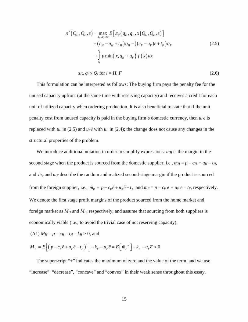
s.t. qi ≤ Qi for i = H, F (2.6)

This formulation can be interpreted as follows: The buying firm pays the penalty fee for the

unused capacity upfront (at the same time with reserving capacity) and receives a credit for each

unit of utilized capacity when ordering production. It is also beneficial to state that if the unit

penalty cost from unused capacity is paid in the buying firm’s domestic currency, then uFe is

replaced with uF in (2.5) and uFē with uF in (2.4); the change does not cause any changes in the

structural properties of the problem.

We introduce additional notation in order to simplify expressions: mH is the margin in the

second stage when the product is sourced from the domestic supplier, i.e., mH = p – cH + uH – tH,

and Fm and mF describe the random and realized second-stage margin if the product is sourced

from the foreign supplier, i.e., F F F Fm p c e u e t= − + − and mF = p – cF e + uF e – tF, respectively.

We denote the first stage profit margins of the product sourced from the home market and

foreign market as MH and MF, respectively, and assume that sourcing from both suppliers is

economically viable (i.e., to avoid the trivial case of not reserving capacity):

(A1) MH = p – cH – tH – kH > 0, and

( ) 0F F F F FF F F Fp c e u e t k u e kE um eM E+ + = − =− + − − −− >

The superscript “+” indicates the maximum of zero and the value of the term, and we use

“increase”, “decrease”, “concave” and “convex” in their weak sense throughout this essay.

16

Note that assumption (A1) is not a restrictive assumption for the foreign supplier as its value is

less than the expected margin (when the firm reserves and utilizes its entire capacity) MF ≥ p – cF

ē – tF – kF.

Our model provides the firm with the flexibility to alter its production orders based on the

realized value of the exchange rate as long as the firm has reserved capacity. The order allocation

flexibility enables the firm to utilize the lower cost supplier. Such variations in the optimal

second-stage decisions influence the first-stage capacity reservation decisions. Thus, both first-

stage capacity reservation and second-stage production decisions are affected by exchange-rate

uncertainty.

The optimal second-stage production decisions can be classified in three regions of

exchange-rate realizations. In the first region the realized exchange rate is so low (el ≤ e ≤ τ1 =

(cH − uH + tH − tF)/(cF − uF)) that sourcing from the foreign supplier (i.e., offshore sourcing) is

less costly than sourcing from the home supplier (i.e., onshore sourcing). In other words, for

these realized values of exchange rates, offshore sourcing is more desirable than onshore

sourcing (i.e., mF ≥ mH > 0). In the second region, the realized exchange rate is higher but not

sufficiently high to cause offshore sourcing to be eliminated from consideration. Specifically, in

this region we have τ1 ≤ e ≤ τ2 = (p − tF)/(cF − uF) corresponding to exchange rate realizations

where onshore sourcing is more profitable than offshore sourcing but offshore sourcing is still

profitable, i.e., mH > mF ≥ 0. In the third and final region, the realized value of the exchange rate

is so high that offshore sourcing is no more a viable alternative, i.e., mF < 0. In this region, the

firm does not order the product from the foreign supplier even if it has already reserved capacity

in the first stage.

17

The threshold point τ1 can be lower or higher than the mean of the exchange rate ē depending

on the relative magnitude of the cost terms. Throughout the manuscript, we do not impose any

assumptions regarding their relative magnitudes. Figure 2.3 illustrates the three regions for an

example where τ1 and τ2 are located within the support of e , i.e., el < (cH − uH + tH − tF)/(cF − uF)

and eh > (p − tF)/(cF − uF).

Figure 2.3. Exchange-rate realization in the second stage.

2.4 Analysis

2.4.1 Demand Uncertainty

We begin our analysis by focusing on the influence of demand uncertainty. We consider the

special case when the exchange-rate random variable is replaced by its deterministic equivalent,

its mean ē. When uncertainty is only associated with demand, the problem becomes a single-

stage Newsvendor Problem with two suppliers. We define the total unit sourcing cost as the sum

of unit capacity reservation, production, transportation, duties and localization costs: cHT = kH +

cH + tH and cFT = kF + cF ē + tF. It is easy to verify that the firm would choose the supplier with

the lowest total unit sourcing cost in this special case. Thus, the firm always chooses the single-

sourcing option. This observation is formalized in following remark that the firm would not

engage in dual sourcing in the absence of exchange-rate uncertainty in our model.

18

Remark 2.1. Demand uncertainty by itself does not lead to dual sourcing in the operating

environment modeled by (2.1)–(2.3).

2.4.2 Demand and Exchange-Rate Uncertainty

The second-stage problem conforms to the standard newsvendor structure with the first-stage

capacity constraints. With no capacity constraints in the second stage, the optimal order

quantities from each supplier can be determined easily by solving two independent Newsvendor

Problems.

2.4.2.1 Onshore Sourcing

If the firm restricts its sourcing activities to an onshore supplier, the problem becomes a

single-stage Newsvendor Problem and exchange-rate uncertainty becomes irrelevant. In Stage 2,

if the firm ignores the first-stage capacity reservation contract, it would order qH0 = F–1((p – cH +

uH – tH)/p) units of products from the onshore source. The optimal amount of capacity reserved

in Stage 1 is:

( )( )0 1 0/H H H H HQ F p k c t p q−= − − − < (2.7)

In other words, when the domestic supplier is the only alternative, the firm utilizes the

reserved capacity in its entirety in the second stage.

2.4.2.2 Offshore Sourcing

If the firm utilizes only the offshore source, then its second-stage production amount is

limited by the amount of capacity reserved in stage 1 (denoted QF) as well as the amount

established by the Newsvendor fractile (denoted qF0(e)). In the absence of a limitation caused by

capacity reservation, the firm would prefer to produce qF0(e) = F–1((p – cFe + uFe – tF)+/p). We

describe the exchange rate threshold value where the firm’s first-stage production amount equals

the desired level of second-stage production amount as τ(QF) = (p[1 – F(QF)] – tF)/(cF – uF). If

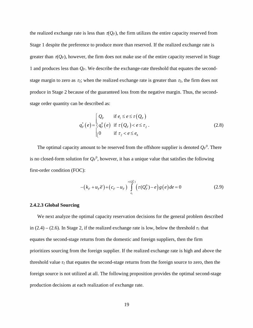
19

the realized exchange rate is less than τ(QF), the firm utilizes the entire capacity reserved from

Stage 1 despite the preference to produce more than reserved. If the realized exchange rate is

greater than τ(QF), however, the firm does not make use of the entire capacity reserved in Stage

1 and produces less than QF. We describe the exchange-rate threshold that equates the second-

stage margin to zero as τ2; when the realized exchange rate is greater than τ2, the firm does not

produce in Stage 2 because of the guaranteed loss from the negative margin. Thus, the second-

stage order quantity can be described as:

( )( )

( ) ( )* 02

2

if

if 0 if

F l F

F F F

h

Q e e Q

q e q e Q ee e

τ

τ τ

τ

≤ ≤= < ≤ < ≤

. (2.8)

The optimal capacity amount to be reserved from the offshore supplier is denoted QF0. There

is no closed-form solution for QF0, however, it has a unique value that satisfies the following

first-order condition (FOC):

( ) ( ) ( ) ( )0( )

0( ) 0F

l

Q

F F F F Fe

k u e c u Q e g e deτ

τ− + + − − =∫ (2.9)

2.4.2.3 Global Sourcing

We next analyze the optimal capacity reservation decisions for the general problem described

in (2.4) – (2.6). In Stage 2, if the realized exchange rate is low, below the threshold τ1 that

equates the second-stage returns from the domestic and foreign suppliers, then the firm

prioritizes sourcing from the foreign supplier. If the realized exchange rate is high and above the

threshold value τ2 that equates the second-stage returns from the foreign source to zero, then the

foreign source is not utilized at all. The following proposition provides the optimal second-stage

production decisions at each realization of exchange rate.

20

Proposition 2.1. The optimal second-stage production decisions are:

( ) ( )( )

( ){ } { }

{ } ( ){ }{ }( )

01

* *1 2

2

0

0 0

0

min , ,min , if

min , ,min , if

min , ,0

( )

, ( )

if

H H F F F l

H F H H F F H

H H h

Q q Q Q q e e

q q Q q Q q Q e

Q q

e

e

e e

e

e

τ

τ τ

τ

+

+

− ≤ < = − ≤ < ≤ ≤

. (2.10)

In the remainder of the essay, we suppress the exchange rate parameter in the optimal second-

stage production functions unless necessary for clarity.

We next establish that the objective function is jointly concave in its decision variables.

Proposition 2.2. The objective function in (2.4) is jointly concave in QH and QF.

From Proposition 2.1, it can be seen that the optimal amount of capacity reserved from the

domestic supplier cannot exceed qH0. The optimal capacity decisions in the first stage can be

classified into the following three sets: Region R1 = {QH, QF│QH + QF ≤ qH0}, region R2 = {QH,

QF│QH ≤ qH0, QF ≤ qH

0 and QH + QF > qH0}, and region R3 = {QH, QF│QH ≤ qH

0 and QF > qH0}.

These three regions are illustrated in Figure 2.4.

Figure 2.4. Optimal regions for the general case of the problem.

21

We can determine the optimal capacity decisions in each of the three regions depicted in

Figure 2.4. From Proposition 2.2, we know that the problem is jointly concave in QH and QF.

Therefore, we can identify optimal decisions in each region through the FOC. The optimal

capacity reservation decisions in region R1 satisfies the following system of equations:

( )( )( ) ( ) ( ) ( )

( )

( )( ) ( )

H

H

h

l

F

eF F F H H H

F F

F F

F Fe

HQ

Q Q

H F

Q

Q

k c e t k c te g e de

c u

k u ee g e deQc u

τ

τ

τ

τ+

+ + − + +− =

−

+ − = −+

∫

∫. (2.11)

Defining the values of τ(QH) and τ (QH + QF) that solve the system of equations (2.11) as τH*

and τHF*, respectively, we can express the optimal capacity choices as follows:

** 1

* ** 1 1

( )

( ) ( )

F F HH

F F HF F F HF

F

F F

p c uQ Fp

p c u p c u

t

tQ F Fp p

t

τ

τ τ

−

− −

− −=

− − − − = −

−

−

−

. (2.12)

The optimal solution is never located in region R2; this is formalized in the following

proposition. Considering the fact that it is never optimal to reserve more capacity than qH0 at the

home country, this proposition guarantees that the capacity to be reserved from the foreign

supplier is either greater than qH0, or it is sufficiently low that the total amount of capacity to be

reserved is not more than qH0.

Proposition 2.3. The optimal solution does not lie in region R2.

The optimal capacity reservation decisions in region R3 satisfies the following system of

equations:

22

( )( )( ) ( )

( )

( )

( )( ) ( )

h

l

H

F

eH F H H

F FH

Q

F F

F Fe

Q

F

E m m k ue g e de

c u

k u ee g ec u

Q

Q de

τ

τ

τ

τ

+ − − − − = − +

− =−

∫

∫

. (2.13)

Describing the values of τ(QH) and τ(QF) that solve (2.13) as τH* and τF

*, respectively we can

express the optimal capacity choices as follows:

** 1

** 1

( )

( )

F F H F

F

H

F F FF

p c uQ Fp

p c u tQp

t

F

τ

τ

−

−

− −=

− − =

−

−

. (2.14)

2.4.3 Optimal Sourcing Policies

We next show that there are five potentially optimal policies: one onshore sourcing, two

offshore sourcing, and two dual sourcing policies. We describe them as follows:

(1) Policy H: Onshore sourcing with QH* = QH

0 and QF* = 0,

(2) Policy FL: Offshore sourcing with a smaller capacity reservation QF* = QF

0 ≤ qH0 and QH

*

= 0,

(3) Policy FH: Offshore sourcing with a higher capacity reservation QF* = QF

0 > qH0 and QH

*

= 0,

(4) Policy DR: Dual sourcing featuring a rationing perspective with QH* + QF

* = QF0,

(5) Policy DE: Dual sourcing featuring excess capacity with QF* = QF

0 and QH* < QH

0.

Policy H is the onshore policy where the firm reserves capacity only at the domestic supplier.

The optimal amount of capacity to reserve is equal to QH* = QH

0 where QH0 is determined

through (2.7). The next two policies, FL and FH, are offshore policies where the optimal capacity

reservation decisions are QF* = QF

0 where QF0 is determined through (2.9). Recall that QF

0 can

23

be less than or greater than qH0. We denote the offshore sourcing policy that leads to limited

capacity investment QF* = QF

0 ≤ qH0 as FL, and the offshore sourcing policy with a higher

capacity commitment QF* = QF

0 > qH0 as FH.

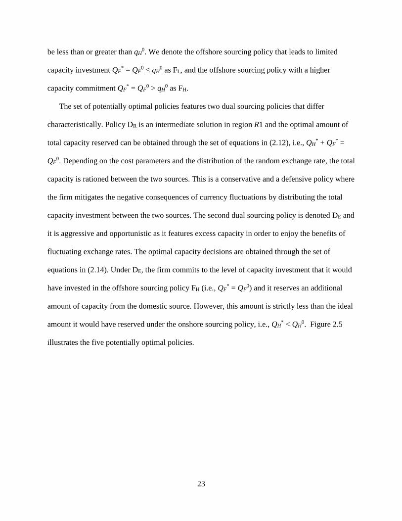
The set of potentially optimal policies features two dual sourcing policies that differ

characteristically. Policy DR is an intermediate solution in region R1 and the optimal amount of

total capacity reserved can be obtained through the set of equations in (2.12), i.e., QH* + QF

* =

QF0. Depending on the cost parameters and the distribution of the random exchange rate, the total

capacity is rationed between the two sources. This is a conservative and a defensive policy where

the firm mitigates the negative consequences of currency fluctuations by distributing the total

capacity investment between the two sources. The second dual sourcing policy is denoted DE and

it is aggressive and opportunistic as it features excess capacity in order to enjoy the benefits of

fluctuating exchange rates. The optimal capacity decisions are obtained through the set of

equations in (2.14). Under DE, the firm commits to the level of capacity investment that it would

have invested in the offshore sourcing policy FH (i.e., QF* = QF

0) and it reserves an additional

amount of capacity from the domestic source. However, this amount is strictly less than the ideal

amount it would have reserved under the onshore sourcing policy, i.e., QH* < QH

0. Figure 2.5

illustrates the five potentially optimal policies.

24

Figure 2.5. Set of all possible optimal solutions.

The above set of potentially optimal policies can be obtained by reviewing four optimality

conditions. These four conditions provide the necessary and sufficient conditions for each policy

to be the optimal decision. These four optimality conditions are:

(OC1): ( ) 0F H F FE m M k u e++ − − − >

,

(OC2): ( ) 0F H F FE m m k u e++ − − − >

,

(OC3): ( ) 0H H H F F Fm k u E m k u e+ − − − − − > ,

(OC4): ( ) 0H F H HE m m k u+ + − − − > .

Proposition 2.4 shows how the five potentially optimal policies are obtained through the

above four optimality conditions.

Proposition 2.4.

(a) Policy H is optimal iff (OC1) does not hold;

25

(b) Policy FL is optimal iff (OC2) and (OC3) do not hold;

(c) Policy FH is optimal iff (OC2) holds and (OC4) does not hold;

(d) Policy DR is optimal iff (OC1) and (OC3) hold and (OC2) does not hold;

(e) Policy DE is optimal iff (OC2) and (OC4) hold.

Table 2.1 presents the necessary and sufficient conditions for each policy to be the optimal

solution for the problem modeled in (2.4) – (2.6). Dual sourcing is the prevailing policy under

certain conditions. The following proposition shows that a quick comparison between the

optimal offshore capacity with the desired level of second-stage order quantity from the domestic

source reveals which one of these two dual sourcing policies can be featured in the optimal

solution. We also observe that QH0 establishes a minimum total capacity reservation amount for

the global sourcing problem (see Lemma 2A.5 in the appendix).

Optimal Sourcing Policy

Optimality Condition

Onshore Sourcing

Offshore Sourcing

Dual Sourcing

H FL FH DR DE

(OC1) × (OC2) × × (OC3) × (OC4) ×

Table 2.1. Necessary and sufficient conditions for the first-stage optimal decisions. A check mark (“”) indicates that the corresponding inequality (i.e., optimality condition) holds when a

particular sourcing policy is optimal, and a cross mark (“×”) indicates that the opposite inequality holds.

Proposition 2.5. (a) If QF0 < qH

0, then policy DE cannot be optimal, leaving policy DR as the

only viable dual sourcing policy; (b) If QF0 > qH

0, then policy DR cannot be optimal, leaving

policy DE as the only viable dual sourcing policy.

26

Dual sourcing policies DR and DE exhibit completely different characteristics. We next

provide a discussion of these two policies.

2.4.3.1 Rationing Dual Sourcing with Policy DR

In policy DR, the firm reserves capacity from both sources where the sum of these reserved

capacities equals the amount of capacity it would have reserved from the offshore source, i.e.,

QH* + QF

* = QF0. The firm’s allocation of capacity can be perceived as rationing capacity in

order to mitigate cost uncertainty stemming from currency fluctuations. In this policy, the firm

does not necessarily benefit much from currency swings. Thus, it is a defensive and a

conservative policy that can be perceived as mitigating the negative consequences of currency

fluctuations. Under DR, the firm always utilizes the home supplier to its maximum, i.e., qH* =

QH* at every realization of the random exchange rate. However, it utilizes the foreign supplier up

to its limit only when the realized exchange rate is desirable, i.e., e ≤ τ1.

According to policy DR, the firm diversifies its supply base between a cost-uncertain and a

cost-certain supplier in order to mitigate the negative consequences of exchange-rate uncertainty.

However, it cannot capitalize completely in the event that exchange rate makes the foreign

supplier an economically desirable source; this can be seen from qF* = QF

0 – QH* < QF

0 when el ≤

e ≤ τ1.

2.4.3.2 Excess Dual Sourcing with Policy DE

Two observations can be made regarding policy DE. First, the firm considers the foreign

supplier as its primary source and reserves the exact amount of capacity it would have reserved

under the offshore sourcing policies, i.e., QF* = QF

0. Second, the firm reserves additional

capacity from the domestic source. However, this amount is strictly less than what it would have

reserved under the onshore sourcing policy, i.e., QH* < QH

0. The domestic supplier appears to

27

serve as a backup source in this policy. The amount reserved at the domestic source QH* is

utilized only when the realized exchange rate makes the foreign source an expensive supplier.

Similarly, the foreign source is not always utilized at its maximum reserved capacity. By

reserving a total capacity that exceeds the optimal amount that would be reserved from the

offshore source, the firm always ends up wasting some reserved capacity, but in turn, takes

advantage of the swings in the exchange rate. Thus, additional capacity reserved at the domestic

source leads to an opportunistic behavior and provides the flexibility to enjoy the benefits of cost

fluctuations.

2.5 The Impact of Exchange-Rate Uncertainty

In this section, we compare the optimal sourcing decisions under exchange-rate and demand

uncertainty with those obtained under deterministic exchange rate and stochastic demand by

replacing the random exchange rate with its deterministic equivalent. The comparison provides

insights regarding the impact of exchange-rate uncertainty on capacity reservation decisions. It is

shown earlier that the firm does not engage in dual sourcing under demand uncertainty in

isolation in our model; it utilizes either the onshore source or the offshore source depending on

the lower total cost of sourcing. We examine the capacity choices under the cases with one

source featuring the lower total sourcing cost.

Case 1: Lower expected cost at the foreign supplier: kF + cFē + tF < kH + cH + tH. When the

foreign supplier has the lower expected total sourcing cost, the firm always chooses offshore

sourcing under deterministic exchange rate. However, this is not necessarily the case if the

exchange rate is uncertain.

28

Proposition 2.6. When the foreign supplier has the lower expected total unit sourcing cost, the

firm utilizes either an offshore sourcing policy (FL or FH) or the dual sourcing policy DE under

exchange-rate and demand uncertainty.

The above proposition implies that lower expected cost of sourcing is not a sufficient

condition for offshore sourcing. More specifically, when the exchange-rate uncertainty is taken

into account, it may be optimal for the firm to utilize dual sourcing, rather than offshore

sourcing, under specific conditions even if the expected total unit sourcing cost is lower for the

foreign supplier.

Case 2: Lower cost at the domestic supplier: kF + cFē + tF ≥ kH + cH + tH. When sourcing from

the domestic supplier is less costly, the firm always chooses onshore sourcing under

deterministic exchange rate. The next proposition indicates that the offshore sourcing policy can

be optimal despite featuring a more expensive foreign supplier.

Proposition 2.7. When the domestic supplier has the lower total unit sourcing cost, offshore

sourcing policies (FL or FH) can be optimal under exchange-rate and demand uncertainty.

Proposition 2.7 shows that it is not necessary to have the lowest total sourcing cost in order to

reserve capacity at a single source. It shows that lower sourcing cost from the domestic supplier

does not eliminate the possibility of offshore sourcing. Alternatively said, offshore sourcing does

not need to feature the lower expected sourcing cost to be the optimal policy. This result

contrasts the common rationale behind offshore sourcing practices that often justify working

with foreign sources because of the lower cost feature. In our finding, however, foreign source is

utilized only when the exchange rate is lower, and thus, the effective cost of utilizing the foreign

source is lower than its expected sourcing cost.

29

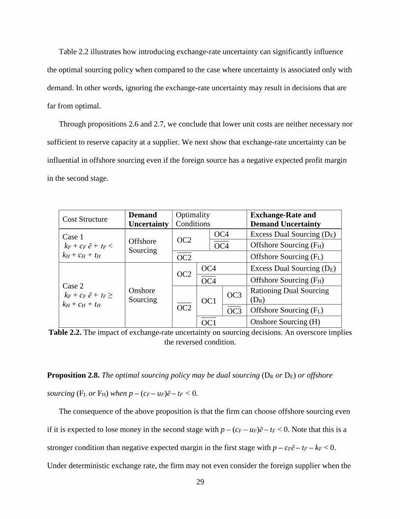
Table 2.2 illustrates how introducing exchange-rate uncertainty can significantly influence

the optimal sourcing policy when compared to the case where uncertainty is associated only with

demand. In other words, ignoring the exchange-rate uncertainty may result in decisions that are

far from optimal.

Through propositions 2.6 and 2.7, we conclude that lower unit costs are neither necessary nor

sufficient to reserve capacity at a supplier. We next show that exchange-rate uncertainty can be

influential in offshore sourcing even if the foreign source has a negative expected profit margin

in the second stage.

Cost Structure Demand Uncertainty

Optimality Conditions

Exchange-Rate and Demand Uncertainty

Case 1 kF + cF ē + tF < kH + cH + tH

Offshore Sourcing

OC2 OC4 Excess Dual Sourcing (DE) OC4 Offshore Sourcing (FH)

OC2 Offshore Sourcing (FL)

Case 2 kF + cF ē + tF ≥ kH + cH + tH

Onshore Sourcing

OC2 OC4 Excess Dual Sourcing (DE) OC4 Offshore Sourcing (FH)

OC2 OC1

OC3 Rationing Dual Sourcing (DR)

OC3 Offshore Sourcing (FL) OC1 Onshore Sourcing (H)

Table 2.2. The impact of exchange-rate uncertainty on sourcing decisions. An overscore implies the reversed condition.

Proposition 2.8. The optimal sourcing policy may be dual sourcing (DR or DE) or offshore

sourcing (FL or FH) when p – (cF – uF)ē – tF < 0.

The consequence of the above proposition is that the firm can choose offshore sourcing even

if it is expected to lose money in the second stage with p – (cF – uF)ē – tF < 0. Note that this is a

stronger condition than negative expected margin in the first stage with p – cFē – tF – kF < 0.

Under deterministic exchange rate, the firm may not even consider the foreign supplier when the

30

second-stage return is negative. Thus, exchange-rate uncertainty creates the opportunity for the

firm to reserve capacity at a supplier even with negative expected margin in the second-stage.

Proposition 2.8 implies that the firm may benefit from giving up a deterministic positive profit

margin from sourcing through the domestic supplier, and instead engage with a single foreign

source even if the expected unit cost from the offshore source (in stage 2) is higher than the unit

price. In this case, postponing the sourcing decision until the revelation of the exchange rate

provides the benefit of potentially high profit margin caused by low exchange-rate realizations. It

also comes at the expense of incurring a potential loss (the sum of capacity reservation cost and

penalty cost of unused capacity) at high realizations of exchange rate. This flexibility can

increase the desirability of the foreign supplier so much that the firm prefers to utilize offshore

sourcing without a domestic supplier even if the foreign supplier has an expected unit cost in

Stage 2 higher than the market price.

We next investigate the impact of exchange-rate volatility on the optimal sourcing policy,

and the expected profit.

Proposition 2.9. (a) The optimal foreign capacity QF* always increases in exchange-rate

volatility. But the optimal domestic capacity QH* may increase or decrease. (b) The expected

profit increases in exchange-rate volatility.

This proposition formally establishes the opportunity that exchange-rate fluctuations along

with the flexibility to postpone the production decisions until realization of the exchange rate can

provide for a firm to improve its expected profit. It is worth noting the asymmetry between the

downside consequences and the upside potential of exchange uncertainty in this business

environment. While lower realizations of the exchange rate lead to higher profits, the amount of

loss due to high realizations is restricted to the total amount of capacity reservation and penalty

31

costs corresponding to the case where the firm does not order production to the foreign supplier.

This asymmetry is key to creating the opportunity to benefit from the higher exchange-rate

volatility.

As for the sourcing decisions, one would intuit that higher degrees of exchange-rate volatility

create the incentive to invest in additional flexibility through domestic capacity. However,

Proposition 2.9 indicates that the optimal domestic capacity does not behave monotonically in

exchange-rate volatility as it may exhibit a decreasing behavior as well. The next proposition

establishes the condition under which the firm indeed reduces its domestic capacity investment

under a uniform exchange-rate distribution.

Proposition 2.10. When the exchange rate is uniformly distributed, under policy DE, the optimal

domestic capacity QH* decreases in exchange-rate volatility iff kH + cH + tH < (cF – uF)ē + tF.

The condition in Proposition 2.10 seems counter-intuitive at first sight as it suggests that

when total unit cost of sourcing from the domestic source is lower than the expected cost of

sourcing from the foreign source, the domestic capacity decreases in exchange-rate uncertainty.

We note that this proposition does not imply that reducing the cost of onshore sourcing leads to

lower optimal capacity at the domestic source. In fact, when kH + cH + tH < (cF – uF)ē + tF, the

firm reserves higher levels of domestic capacity at any degree of exchange-rate volatility

compared to the opposite case (i.e., kH + cH + tH > (cF – uF)ē + tF). The condition in Proposition

2.10 requires that the cost of sourcing from the domestic source is low, and thus, the firm has

already reserved a sufficiently high level of domestic capacity under policy DE. Consequently,

the domestic capacity becomes a substitute for the foreign capacity which increases in exchange-

rate volatility (according to Proposition 2.9). As a result, the firm reduces its high capacity

32

commitment to the domestic source in order to capitalize more on the prospects of sourcing from

the foreign supplier.

The following proposition sheds light on how the optimal sourcing policy evolves with

exchange-rate volatility.

Proposition 2.11. As the exchange-rate volatility increases:

(a) if kF + cFē + tF < kH + cH + tH, then the optimal sourcing policy changes according to the

following path (or a continuous portion thereof): FLFHDE;

(b) if kF + cFē + tF ≥ kH + cH + tH, then the optimal sourcing policy changes according to the

following paths (or a continuous portion thereof): HDR FLFHDE, or HDRDE.

Proposition 2.11 establishes the optimal policy paths that the firm follows as exchange-rate

volatility increases. Specifically, when the foreign supplier is associated with lower expected unit

sourcing cost, the firm either keeps offshore sourcing or switches to policy DE utilizing excess

capacity. On the other hand, when the unit cost of sourcing from the domestic supplier is lower,

the firm switches from onshore sourcing to the dual sourcing policy exhibiting rationing

behavior (DR). With increasing exchange-rate volatility the firm either directly switches to the

excess dual sourcing policy (DE) or first adopts offshore sourcing policies before implementing

the excess dual sourcing policy. We observe that as the degree of exchange-rate variation

increases, the foreign supplier becomes a more desirable supplier. As mentioned before, this is

because there are higher chances of a large savings due to low realization of the exchange rate

while the possible loss due to the appreciation of the exchange rate—which is as much as the

capacity reservation cost plus the penalty cost of unused capacity—remains unchanged.

Consequently, high volatility of exchange rate results in choosing the foreign supplier as the

primary source (corresponding to policies FL, FH, and DE).

33

2.6 Risk Aversion

This section presents the influence of risk aversion on the part of the buying firm. We utilize

the value-at-risk (VaR) measure to limit the risk associated with the realized profits in the global

sourcing problem under exchange-rate and demand uncertainty. VaR is the most widely

employed risk measure in practice and is the prevailing risk approach in the Basel II and III

Accords specifying the banking laws and regulations issued by the Basel Committee on Banking

Supervision (2013). There are two parameters that describe the firm’s risk preferences in VaR: β

≥ 0 represents the loss (value at risk) that the firm is willing to tolerate at probability α, where 0

≤ α ≤ 1. For a given α, if VaR is more than the tolerable loss β, then first-stage decisions (QH,

QF) correspond to an infeasible solution. We incorporate the firm’s VaR concern into the model

in (2.1) – (2.3) by supplementing the first-stage problem with the following probability

constraint:

( ) ( ), ,H Fe x Q QP β α < − ≤Π (2.15)

where

( ) ( ) ( ) ( ) ( )

( )( ) ( )( ) ( ) ( ){ }

* *

* * * * min ,

,H F H H F F H H H F F F

H H H F F F H F

Q Q k Q k Q c t q e c e t q e

u Q q e u e Q q e p x q e q e+ +

Π = − − − + − +

− − − − + +

is the random profit from the optimal second-stage decisions and first-stage capacity reservation

decisions (QH, QF) and ( ) [ ],e xP ⋅ represents the probability over the exchange-rate and demand

random variables. Constraint (2.15) states that the probability that the realized loss exceeds β

should be less than or equal to the firm’s tolerable loss probability α.

Before proceeding with the analysis of risk aversion, it is important to make several

observations. In the absence of exchange-rate uncertainty, the introduction of risk aversion

through a VaR constraint as in (2.15) does not lead to dual sourcing. It is already pointed out

34

earlier that when random exchange rate is replaced with its certainty equivalent ē in the risk-

neutral setting, the firm works with only one supplier and reserves capacity at the lower cost

source. Moreover, the second-stage production amount is always equal to the amount reserved

from Stage 1 as long as the firm operates with positive margins. When the optimal capacity

reserved at the low-cost source (let us denote it with QN) violates the VaR constraint due to the

stochastic demand, then the firm would reduce its initial capacity reservation to satisfy the

constraint at the tolerated loss. Specifically, let xα denote the value of the demand random

variable that corresponds to α probability in its cdf. It is sufficient to check the value of the

realized profit at xα from reserving QN units of capacity at the low cost supplier j: If p xα – (kj + cj

+ tj)QN < – β, then the firm reduces its initial capacity investment from QN to QA = (p xα – β)/(kj

+ cj + tj) where QA describes the amount of capacity reserved in Stage 1 due to risk aversion.

Thus, in the absence of exchange-rate uncertainty, the firm reduces its initial capacity reservation

commitment as a result of risk aversion but does not switch to dual sourcing.

We next examine the impact of risk aversion in the presence of exchange-rate uncertainty.

Let eα denote the exchange rate realization at fractile 1 – α (i.e., [1 – G(eα)] = α). Because

demand uncertainty in isolation does not lead to any policy change in our model, but rather a

reduction in reserved capacity, we focus on problem settings where exchange-rate is a source of

uncertainty in violating the VaR requirement with eα > τ2. Exchange-rate realizations greater than

τ2 are most detrimental to the firm because it would waste the entire capacity reserved at the

foreign source due to the fact that qF*(e) = 0 for e ≥ τ2.

In the presence of exchange-rate uncertainty, incorporating risk aversion encourages the firm

to engage in dual sourcing. This can be seen when the optimal policy in the risk-neutral setting is

an offshore sourcing policy as in the case of policies FH and FL. When risk aversion is included

35

and the VaR constraint is violated, the firm can decrease the level of capacity investment in the

foreign source in order to comply with the VaR constraint in (2.15). Let us define QFA as the

level of capacity reserved at the foreign source that yields realized profit equal to –β at

exchange-rate realization eα, i.e.,

( )AF F FQ k u eαβ= + . (2.16)

We use the following two conditions in Proposition 2.12, which characterizes when the firm

switches from single sourcing at the foreign source (i.e., offshore sourcing policies FH and FL) to

dual sourcing:

(RA1): ( )( )

( )1

AF

l

H H

Q

F FH

F FH F

e

c uM k u E m mG e dek u e

τ

+ + − − > + − − +

∫ ,

(RA2): ( )( )

( ) ( )( )

1

A AF F

l l

Q Q

FF H

FH F

F e eF

F

c uM G E m Me de G e ek

c du e

uτ τ

+ − − >

− −+

− ∫ ∫ .

Proposition 2.12. Suppose the risk-neutral optimal solution violates the VaR constraint, and eα

≥ τ2, uF > 0.

(a) When the optimal sourcing policy in the risk-neutral setting is FH and AFQ > qH

0, the firm

switches to dual sourcing under risk aversion if RA1 holds;

(b) When the optimal sourcing policy in the risk-neutral setting is either FL or FH with AFQ ≤ qH

0,

the firm switches to dual sourcing under risk aversion if RA2 holds.

From Proposition 2.12, we see conditions that cause the firm to switch from offshore

sourcing policies that are optimal in a risk-neutral setting to dual sourcing. Condition RA1 is a

stronger condition because the right hand side (RHS) of RA1 is greater than that of RA2 when

AFQ > qH

0. In this case, when RA1 holds, condition RA2 also holds. Thus, RA1 can be perceived

36

as a sufficient condition that, when an offshore sourcing policy is optimal in the risk-neutral

setting, then the firm switches to dual sourcing as a consequence of risk aversion. It can also be

shown that when dual sourcing policies are optimal in the risk-neutral setting, they continue to be

optimal under risk aversion in our model. In conclusion, our analysis shows that the introduction

of risk aversion through a VaR constraint leads to a higher likelihood of dual sourcing.

2.7 Financial Hedging

We next examine the impact of introducing the flexibility to purchase financial hedging

instruments on the firm’s risk concern and expected profit. We consider the case when the firm

obtains a certain number of currency futures contracts, denoted H, in stage 1 along with its

capacity reservation decisions (QH, QF). Each unit of financial hedging contract has a unit cost of

h(es) (also referred to as the premium) and a strike (or, exercise) price of es. We assume that the

financial institution sells the hedging instrument at cost, i.e.,

( ) ( ) ( ) ( ) ( )h s

s l

e e

s s se e

h e e e g e de e e g e de= − − −∫ ∫ . (2.17)

In Stage 1, the firm now determines the optimal values of (QH, QF, H) in order to maximize

the expected profit subject to the same VaR requirement:

( ) ( ) ( ) ( )*

, , 0, ,max ,, ,

Hl

F

h

H F H H F F H FQ Qe

H

e

sH h e H H e g e dE Q Q k Q k Q Q Q eπ≥

− +Π = − − ∫ . (2.18)

In Stage 2, all financial hedging contracts purchased in Stage 1 are exercised. Subject to the

same capacity reservation constraint in (2.3), the second-stage objective function in (2.2) is then

revised as follows:

37

( ) ( )

( ) ( )

( ) { } ( )

*2, 0

, max , | ,

+ min ,

, , , , ,H F

h

l

H F H F H Fq q

H H F F H H F F H H H F F F

x

s H Fx

Q Q E q q Q Q

c q c eq t q t q

H e x H

u Q q u e Q q

e e H p x q q f x dx

eπ π

+ +

≥ =

= − − − − − − − −

− + +∫

(2.19)

The objective function in (2.19) adds the term (e – es)H into (2.2). The advantage of

employing financial hedging in Stage 1 enables the firm to eliminate the negative consequences

of the VaR constraint in (2.15), which can now be expressed as follows:

( )

( ) ( ) ( ) ( ) ( )

( )( ) ( )( )( ) ( ) ( ){ }

* *

* *,

* *min ,

H H F F H H H F F F

H H H F F F

s H F

s

e x

k Q k Q c t q e c e t q e

u Q q e u e Q q e

e e H p x q e q e

h e H

P β α+ +

− − − + − + − − − −

− < −

≤

+ − + +

. (2.20)

The firm’s tolerated loss probability α is not exceeded when the firm is ensured to have

realized profits greater than or equal to –β when the exchange-rate random variable takes values

in the range el ≤ e ≤ eα. For any given (QH, QF), if the VaR constraint in (2.15) is violated, then

the firm determines the number of hedging contracts that would satisfy the same risk concern

expressed in (2.20) even at the lowest second-stage revenues occurring at x = xl. This is

formalized in the next proposition.

Proposition 2.13. If the first-stage decisions (QH, QF) does not satisfy the VaR constraint in

(2.15) then

(a) the firm can purchase the following number of financial hedging contracts with a strike price

es ≤ eα and premium h(es) as defined in (2.17)

( )

( ) ( ) ( ) ( )

( ) ( ){ } ( )( ) ( )( )( )( )

* *

* * * **

min ,

H H F F H H H F F F

sl H F H H H F F

s s

F

k Q k Q c t q e c e t q e

p x q e q e u Q q e u e Q q e

eH e

h ee

α α α

α α α α α

α

β+ +

+ + + + +

− + − + − + − =

− − (2.21)

and satisfy (2.20); and

38

(b) the expected profit E[Π(QH, QF, H*(es))] under risk aversion and financial hedging is

equivalent to E[Π(QH, QF, 0)] of the risk-neutral setting in the absence of the VaR constraint

(2.15).

Proposition 2.13(a) shows that financial hedging enables the firm to satisfy the VaR

constraint. The number of hedging contracts specified in (2.21) accounts for the losses that can

incur at all of the undesirable exchange-rate realizations in the range of eα ≤ e ≤ eh corresponding

to α percent in the cdf. Thus, the number of financial hedging contracts in (2.21) guarantees that

the firm’s losses exceeding β is less than or equal to the firm’s tolerated loss probability α.

Proposition 2.13(b) shows that financial hedging is also beneficial in terms of protecting the

expected profit. For any capacity reservation decisions (QH, QF) in stage 1, financial hedging

enables the firm to obtain the same expected profit it earned in the risk-neutral setting without

having to sacrifice initial capacity reservation in order to satisfy the VaR constraint.

The consequence of Proposition 2.13(b) is that the firm’s set of potential optimal policies under

risk aversion and financial hedging is identical to the set of policies developed in Section 2.4 for

the risk-neutral setting. Thus, we conclude that financial hedging not only eliminates the

negative consequences of risk aversion, but also makes our five potentially optimal policies to

hold under more general settings.

In sum, we find that our insights into the role of exchange rate uncertainty on optimal

sourcing decisions are robust; we find that the introduction of risk aversion via a VaR constraint

can make dual sourcing more likely and that our conclusions are unaffected by the use of

financial hedging to mitigate risk.

39

2.8 Numerical Illustration

In this section, we provide numerical illustrations from the operating environment of the

furniture manufacturer that motivated our study. For this furniture company specializing in

school and library furniture, there are three selling season, each representing a four-month time

window (following the traditional school semesters). The furniture maker develops a forecast for

its products for each selling season (for four months). The firm makes capacity reservation

decisions one selling season in advance. Book carts, one of the firm’s best known products, are

sourced from small suppliers that charge a unit capacity reservation cost ranging from 1% to 5%

of the selling price. The firm has other products where the unit capacity reservation cost is

between 5% and 10% of the selling price (e.g., office desks and chairs). We present the results

associated with surprising insights, and ignore the expected results associated with product with

higher unit capacity reservation costs.

The capacity reservation payment is made at the spot exchange rate one season before the

selling season approaches (equivalent to four months). Thus, it can be converted to domestic

currency using the spot exchange rate at the time of the initial payment. Four months later,

corresponding to the beginning of the selling season, the furniture maker specifies the exact

amount of products to be manufactured at each supplier. It is important to note that the firm

continues to operate under demand uncertainty during the selling season; schools and libraries

continue to place orders during the selling season.

We next describe the data used to represent exchange-rate fluctuations. Our analysis uses

data on the daily Euro-Dollar exchange rate from the beginning of 2010 through the end of 2012

(3-year period), corresponding to the planning period for the furniture maker that motivated our

problem. We first analyze the rate of change in the exchange rate in four months. We accomplish

40

this goal by examining each daily exchange rate (or, spot rate), denoted st, and comparing it with

the daily exchange rate of four months later, denoted st+120, within our three-year data set.

Specifically, for each day over the 3-year period, we calculate the proportion of the exchange-

rate four months into the future relative to the current exchange rate, i.e., et = st+120/st. The

comparison of the daily exchange rate with its counterpart in four months results in an empirical

distribution which we use in our analysis. Figure 2.6(a) provides the histogram of the empirical

distribution representing the fluctuations in the Euro-Dollar exchange rate used in our numerical

illustrations. Figure 2.6(b) shows the frequency distribution of the change in the value of the

exchange rate in four months. As can be seen from Figure 2.6(b), there would not be a well-

fitting statistical distribution to represent the change in exchange rates in four months. Therefore,

we use the entire data set of the changes during the period of 2010 – 2012 as our distribution in

the analysis.

In order to provide a meaningful and comparative analysis without revealing costs and prices,

we normalize the selling price to $100, and scale the capacity reservation and transportation

costs accordingly. Figure 2.7 demonstrates the optimal decisions with changing values of the

second-stage operational costs, cH and cF, as described in horizontal and vertical axes,

respectively. The unit capacity reservation costs, kH and kF, are smallest in Figure 2.7(a), at 1%

of the selling price, and their values increase in figures 2.7(b) and 2.7(c) up to 5% of the selling

price. The same policy indicators, {H, FL, FH, DR, DE}, are used to designate the five potentially

optimal policies identified in Section 2.4.

41

Figure 2.6. The Euro-Dollar exchange rate between 2010 – 2012. (a) Histogram of the actual

values representing the variation in the Euro-Dollar exchange rate. (b) Frequency distribution of the proportions representing the change in the value of the exchange rate in four months.

(a) kH = $1, kF = $1

01020304050607080

1.2

1.23

1.26

1.29

1.32

1.35

1.38

1.41

1.44

1.47 1.

5

Freq

uenc

y

Euro-Dollar exchange ratesmean = 1.335, standard deviation = 0.065

01020304050607080

0.85

0.88

0.91

0.94

0.97 1

1.03

1.06

1.09

1.12

1.15

Freq

uenc

y

Proportions (St+120 / St )mean = 0.995, standard deviation = 0.060

0.0 60.0 60.5 61.0 61.5 62.0 62.5 63.0 63.5 64.0 64.5 65.0 65.5 66.0 66.5 67.0 67.5 68.0 68.5 69.0 69.5 70.0 70.5 71.0 71.5 72.0 72.5 73.0 73.5 74.0 74.5 75.0 75.5 76.0 76.5 77.0 77.5 78.0 78.5 79.0 79.5 80.0 80.5 81.0 81.5 82.0 82.5 83.0 83.5 84.0 84.5 85.0 85.5 86.0 86.5 87.0 87.5 88.0 88.5 89.0 89.5 90.060.0 DE FH FH FH FH FH FH FH FH FH FH FH FH FH FH FH FH FH FH FH FH FH FH FH FH FH FH FH FH FH FH FH FH FH FH FH FH FH FH FH FH FH FH FH FH FH FH FH FH FH FH FH FH FH FH FH FH FH FH FH FH60.5 DE DE FH FH FH FH FH FH FH FH FH FH FH FH FH FH FH FH FH FH FH FH FH FH FH FH FH FH FH FH FH FH FH FH FH FH FH FH FH FH FH FH FH FH FH FH FH FH FH FH FH FH FH FH FH FH FH FH FH FH FH61.0 DE DE DE FH FH FH FH FH FH FH FH FH FH FH FH FH FH FH FH FH FH FH FH FH FH FH FH FH FH FH FH FH FH FH FH FH FH FH FH FH FH FH FH FH FH FH FH FH FH FH FH FH FH FH FH FH FH FH FH FH FH61.5 DE DE DE DE FH FH FH FH FH FH FH FH FH FH FH FH FH FH FH FH FH FH FH FH FH FH FH FH FH FH FH FH FH FH FH FH FH FH FH FH FH FH FH FH FH FH FH FH FH FH FH FH FH FH FH FH FH FH FH FH FH62.0 DE DE DE DE DE FH FH FH FH FH FH FH FH FH FH FH FH FH FH FH FH FH FH FH FH FH FH FH FH FH FH FH FH FH FH FH FH FH FH FH FH FH FH FH FH FH FH FH FH FH FH FH FH FH FH FH FH FH FH FH FH62.5 DR DE DE DE DE DE FH FH FH FH FH FH FH FH FH FH FH FH FH FH FH FH FH FH FH FH FH FH FH FH FH FH FH FH FH FH FH FH FH FH FH FH FH FH FH FH FH FH FH FH FH FH FH FH FH FH FH FH FH FH FH63.0 DR DR DE DE DE DE DE FH FH FH FH FH FH FH FH FH FH FH FH FH FH FH FH FH FH FH FH FH FH FH FH FH FH FH FH FH FH FH FH FH FH FH FH FH FH FH FH FH FH FH FH FH FH FH FH FH FH FH FH FH FH63.5 H DR DR DE DE DE DE DE FH FH FH FH FH FH FH FH FH FH FH FH FH FH FH FH FH FH FH FH FH FH FH FH FH FH FH FH FH FH FH FH FH FH FH FH FH FH FH FH FH FH FH FH FH FH FH FH FH FH FH FH FH64.0 H H DR DR DE DE DE DE DE FH FH FH FH FH FH FH FH FH FH FH FH FH FH FH FH FH FH FH FH FH FH FH FH FH FH FH FH FH FH FH FH FH FH FH FH FH FH FH FH FH FH FH FH FH FH FH FH FH FH FH FH64.5 H H H DR DR DE DE DE DE DE FH FH FH FH FH FH FH FH FH FH FH FH FH FH FH FH FH FH FH FH FH FH FH FH FH FH FH FH FH FH FH FH FH FH FH FH FH FH FH FH FH FH FH FH FH FH FH FH FH FH FH65.0 H H H H DR DR DE DE DE DE DE FH FH FH FH FH FH FH FH FH FH FH FH FH FH FH FH FH FH FH FH FH FH FH FH FH FH FH FH FH FH FH FH FH FH FH FH FH FH FH FH FH FH FH FH FH FH FH FH FH FH65.5 H H H H H DR DR DE DE DE DE DE DE FH FH FH FH FH FH FH FH FH FH FH FH FH FH FH FH FH FH FH FH FH FH FH FH FH FH FH FH FH FH FH FH FH FH FH FH FH FH FH FH FH FH FH FH FH FH FH FH66.0 H H H H H H DR DR DE DE DE DE DE DE FH FH FH FH FH FH FH FH FH FH FH FH FH FH FH FH FH FH FH FH FH FH FH FH FH FH FH FH FH FH FH FH FH FH FH FH FH FH FH FH FH FH FH FH FH FH FH66.5 H H H H H H H DR DR DE DE DE DE DE DE FH FH FH FH FH FH FH FH FH FH FH FH FH FH FH FH FH FH FH FH FH FH FH FH FH FH FH FH FH FH FH FH FH FH FH FH FH FH FH FH FH FH FH FH FH FH67.0 H H H H H H H H DR DR DE DE DE DE DE DE FH FH FH FH FH FH FH FH FH FH FH FH FH FH FH FH FH FH FH FH FH FH FH FH FH FH FH FH FH FH FH FH FH FH FH FH FH FH FH FH FH FH FH FH FH67.5 H H H H H H H H H DR DR DE DE DE DE DE DE FH FH FH FH FH FH FH FH FH FH FH FH FH FH FH FH FH FH FH FH FH FH FH FH FH FH FH FH FH FH FH FH FH FH FH FH FH FH FH FH FH FH FH FH68.0 H H H H H H H H H H DR DR DE DE DE DE DE DE FH FH FH FH FH FH FH FH FH FH FH FH FH FH FH FH FH FH FH FH FH FH FH FH FH FH FH FH FH FH FH FH FH FH FH FH FH FH FH FH FH FH FH68.5 H H H H H H H H H H H DR DR DE DE DE DE DE DE FH FH FH FH FH FH FH FH FH FH FH FH FH FH FH FH FH FH FH FH FH FH FH FH FH FH FH FH FH FH FH FH FH FH FH FH FH FH FH FH FH FH69.0 H H H H H H H H H H H DR DR DE DE DE DE DE DE DE FH FH FH FH FH FH FH FH FH FH FH FH FH FH FH FH FH FH FH FH FH FH FH FH FH FH FH FH FH FH FH FH FH FH FH FH FH FH FH FH FH69.5 H H H H H H H H H H H H DR DR DE DE DE DE DE DE DE FH FH FH FH FH FH FH FH FH FH FH FH FH FH FH FH FH FH FH FH FH FH FH FH FH FH FH FH FH FH FH FH FH FH FH FH FH FH FH FH70.0 H H H H H H H H H H H H H DR DR DE DE DE DE DE DE DE FH FH FH FH FH FH FH FH FH FH FH FH FH FH FH FH FH FH FH FH FH FH FH FH FH FH FH FH FH FH FH FH FH FH FH FH FH FH FH70.5 H H H H H H H H H H H H H H DR DR DE DE DE DE DE DE DE FH FH FH FH FH FH FH FH FH FH FH FH FH FH FH FH FH FH FH FH FH FH FH FH FH FH FH FH FH FH FH FH FH FH FH FH FH FH71.0 H H H H H H H H H H H H H H H DR DR DE DE DE DE DE DE DE FH FH FH FH FH FH FH FH FH FH FH FH FH FH FH FH FH FH FH FH FH FH FH FH FH FH FH FH FH FH FH FH FH FH FH FH FH71.5 H H H H H H H H H H H H H H H H DR DR DE DE DE DE DE DE DE FH FH FH FH FH FH FH FH FH FH FH FH FH FH FH FH FH FH FH FH FH FH FH FH FH FH FH FH FH FH FH FH FH FH FH FH72.0 H H H H H H H H H H H H H H H H H DR DR DE DE DE DE DE DE DE FH FH FH FH FH FH FH FH FH FH FH FH FH FH FH FH FH FH FH FH FH FH FH FH FH FH FH FH FH FH FH FH FH FH FH72.5 H H H H H H H H H H H H H H H H H H DR DR DE DE DE DE DE DE DE FH FH FH FH FH FH FH FH FH FH FH FH FH FH FH FH FH FH FH FH FH FH FH FH FH FH FH FH FH FH FH FH FH FH73.0 H H H H H H H H H H H H H H H H H H H DR DR DE DE DE DE DE DE DE DE FH FH FH FH FH FH FH FH FH FH FH FH FH FH FH FH FH FH FH FH FH FH FH FH FH FH FH FH FH FH FH FH73.5 H H H H H H H H H H H H H H H H H H H H DR DR DE DE DE DE DE DE DE DE FH FH FH FH FH FH FH FH FH FH FH FH FH FH FH FH FH FH FH FH FH FH FH FH FH FH FH FH FH FH FH74.0 H H H H H H H H H H H H H H H H H H H H H DR DR DE DE DE DE DE DE DE DE FH FH FH FH FH FH FH FH FH FH FH FH FH FH FH FH FH FH FH FH FH FH FH FH FH FH FH FH FH FH74.5 H H H H H H H H H H H H H H H H H H H H H H DR DR DE DE DE DE DE DE DE DE FH FH FH FH FH FH FH FH FH FH FH FH FH FH FH FH FH FH FH FH FH FH FH FH FH FH FH FH FH75.0 H H H H H H H H H H H H H H H H H H H H H H H DR DR DE DE DE DE DE DE DE DE FH FH FH FH FH FH FH FH FH FH FH FH FH FH FH FH FH FH FH FH FH FH FH FH FH FH FH FH75.5 H H H H H H H H H H H H H H H H H H H H H H H H DR DR DE DE DE DE DE DE DE DE FH FH FH FH FH FH FH FH FH FH FH FH FH FH FH FH FH FH FH FH FH FH FH FH FH FH FH76.0 H H H H H H H H H H H H H H H H H H H H H H H H H DR DR DE DE DE DE DE DE DE DE FH FH FH FH FH FH FH FH FH FH FH FH FH FH FH FH FH FH FH FH FH FH FH FH FH FH76.5 H H H H H H H H H H H H H H H H H H H H H H H H H H DR DR DE DE DE DE DE DE DE DE FH FH FH FH FH FH FH FH FH FH FH FH FH FH FH FH FH FH FH FH FH FH FH FH FH77.0 H H H H H H H H H H H H H H H H H H H H H H H H H H H DR DR DE DE DE DE DE DE DE DE FH FH FH FH FH FH FH FH FH FH FH FH FH FH FH FH FH FH FH FH FH FH FH FH77.5 H H H H H H H H H H H H H H H H H H H H H H H H H H H DR DR DE DE DE DE DE DE DE DE DE FH FH FH FH FH FH FH FH FH FH FH FH FH FH FH FH FH FH FH FH FH FH FH78.0 H H H H H H H H H H H H H H H H H H H H H H H H H H H H DR DR DE DE DE DE DE DE DE DE DE FH FH FH FH FH FH FH FH FH FH FH FH FH FH FH FH FH FH FH FH FH FH78.5 H H H H H H H H H H H H H H H H H H H H H H H H H H H H H DR DR DE DE DE DE DE DE DE DE DE FH FH FH FH FH FH FH FH FH FH FH FH FH FH FH FH FH FH FH FH FH79.0 H H H H H H H H H H H H H H H H H H H H H H H H H H H H H H DR DR DE DE DE DE DE DE DE DE DE FH FH FH FH FH FH FH FH FH FH FH FH FH FH FH FH FH FH FH FH79.5 H H H H H H H H H H H H H H H H H H H H H H H H H H H H H H H DR DR DE DE DE DE DE DE DE DE DE FH FH FH FH FH FH FH FH FH FH FH FH FH FH FH FH FH FH FH80.0 H H H H H H H H H H H H H H H H H H H H H H H H H H H H H H H H DR DR DE DE DE DE DE DE DE DE DE FH FH FH FH FH FH FH FH FH FH FH FH FH FH FH FH FH FH80.5 H H H H H H H H H H H H H H H H H H H H H H H H H H H H H H H H H DR DR DE DE DE DE DE DE DE DE DE DE FH FH FH FH FH FH FH FH FH FH FH FH FH FH FH FH81.0 H H H H H H H H H H H H H H H H H H H H H H H H H H H H H H H H H H DR DR DE DE DE DE DE DE DE DE DE DE FH FH FH FH FH FH FH FH FH FH FH FH FH FH FH81.5 H H H H H H H H H H H H H H H H H H H H H H H H H H H H H H H H H H H DR DR DE DE DE DE DE DE DE DE DE DE FH FH FH FH FH FH FH FH FH FH FH FH FH FH82.0 H H H H H H H H H H H H H H H H H H H H H H H H H H H H H H H H H H H H DR DR DE DE DE DE DE DE DE DE DE DE FH FH FH FH FH FH FH FH FH FH FH FH FH82.5 H H H H H H H H H H H H H H H H H H H H H H H H H H H H H H H H H H H H H DR DR DE DE DE DE DE DE DE DE DE DE FH FH FH FH FH FH FH FH FH FH FH FH83.0 H H H H H H H H H H H H H H H H H H H H H H H H H H H H H H H H H H H H H H DR DR DE DE DE DE DE DE DE DE DE DE FH FH FH FH FH FH FH FH FH FH FH83.5 H H H H H H H H H H H H H H H H H H H H H H H H H H H H H H H H H H H H H H H DR DR DE DE DE DE DE DE DE DE DE DE FH FH FH FH FH FH FH FH FH FH84.0 H H H H H H H H H H H H H H H H H H H H H H H H H H H H H H H H H H H H H H H H DR DR DE DE DE DE DE DE DE DE DE DE FH FH FH FH FH FH FH FH FH84.5 H H H H H H H H H H H H H H H H H H H H H H H H H H H H H H H H H H H H H H H H H DR DR DE DE DE DE DE DE DE DE DE FH FH FH FH FH FH FH FH FH85.0 H H H H H H H H H H H H H H H H H H H H H H H H H H H H H H H H H H H H H H H H H H DR DR DE DE DE DE DE DE DE DE FH FH FH FH FH FH FH FH FH85.5 H H H H H H H H H H H H H H H H H H H H H H H H H H H H H H H H H H H H H H H H H H DR DR DE DE DE DE DE DE DE DE DE FH FH FH FH FH FH FH FH86.0 H H H H H H H H H H H H H H H H H H H H H H H H H H H H H H H H H H H H H H H H H H H DR DR DE DE DE DE DE DE DE DE DE FH FH FH FH FH FH FH86.5 H H H H H H H H H H H H H H H H H H H H H H H H H H H H H H H H H H H H H H H H H H H H DR DR DE DE DE DE DE DE DE DE FH FH FH FH FH FH FH87.0 H H H H H H H H H H H H H H H H H H H H H H H H H H H H H H H H H H H H H H H H H H H H H DR DR DE DE DE DE DE DE DE DE FH FH FH FH FH FH87.5 H H H H H H H H H H H H H H H H H H H H H H H H H H H H H H H H H H H H H H H H H H H H H H DR DR DE DE DE DE DE DE DE DE FH FH FH FH FH88.0 H H H H H H H H H H H H H H H H H H H H H H H H H H H H H H H H H H H H H H H H H H H H H H H DR DR DE DE DE DE DE DE DE DE FH FH FH FH88.5 H H H H H H H H H H H H H H H H H H H H H H H H H H H H H H H H H H H H H H H H H H H H H H H H DR DR DE DE DE DE DE DE DE FH FH FH FH89.0 H H H H H H H H H H H H H H H H H H H H H H H H H H H H H H H H H H H H H H H H H H H H H H H H H DR DR DE DE DE DE DE DE DE FH FH FH89.5 H H H H H H H H H H H H H H H H H H H H H H H H H H H H H H H H H H H H H H H H H H H H H H H H H H DR DR DE DE DE DE DE DE DE FH FH90.0 H H H H H H H H H H H H H H H H H H H H H H H H H H H H H H H H H H H H H H H H H H H H H H H H H H H DR DR DE DE DE DE DE DE FH FH

CH

CF

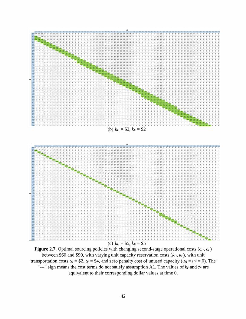
42

(b) kH = $2, kF = $2

(c) kH = $5, kF = $5

Figure 2.7. Optimal sourcing policies with changing second-stage operational costs (cH, cF) between $60 and $90, with varying unit capacity reservation costs (kH, kF), with unit

transportation costs tH = $2, tF = $4, and zero penalty cost of unused capacity (uH = uF = 0). The “---“ sign means the cost terms do not satisfy assumption A1. The values of kF and cF are

equivalent to their corresponding dollar values at time 0.

0.0 60.0 60.5 61.0 61.5 62.0 62.5 63.0 63.5 64.0 64.5 65.0 65.5 66.0 66.5 67.0 67.5 68.0 68.5 69.0 69.5 70.0 70.5 71.0 71.5 72.0 72.5 73.0 73.5 74.0 74.5 75.0 75.5 76.0 76.5 77.0 77.5 78.0 78.5 79.0 79.5 80.0 80.5 81.0 81.5 82.0 82.5 83.0 83.5 84.0 84.5 85.0 85.5 86.0 86.5 87.0 87.5 88.0 88.5 89.0 89.5 90.060.0 FH FH FH FH FH FH FH FH FH FH FH FH FH FH FH FH FH FH FH FH FH FH FH FH FH FH FH FH FH FH FH FH FH FH FH FH FH FH FH FH FH FH FH FH FH FH FH FH FH FH FH FH FH FH FH FH FH FH FH FH FH60.5 FL FH FH FH FH FH FH FH FH FH FH FH FH FH FH FH FH FH FH FH FH FH FH FH FH FH FH FH FH FH FH FH FH FH FH FH FH FH FH FH FH FH FH FH FH FH FH FH FH FH FH FH FH FH FH FH FH FH FH FH FH61.0 DR FL FH FH FH FH FH FH FH FH FH FH FH FH FH FH FH FH FH FH FH FH FH FH FH FH FH FH FH FH FH FH FH FH FH FH FH FH FH FH FH FH FH FH FH FH FH FH FH FH FH FH FH FH FH FH FH FH FH FH FH61.5 DR DR FL FH FH FH FH FH FH FH FH FH FH FH FH FH FH FH FH FH FH FH FH FH FH FH FH FH FH FH FH FH FH FH FH FH FH FH FH FH FH FH FH FH FH FH FH FH FH FH FH FH FH FH FH FH FH FH FH FH FH62.0 DR DR DR FL FH FH FH FH FH FH FH FH FH FH FH FH FH FH FH FH FH FH FH FH FH FH FH FH FH FH FH FH FH FH FH FH FH FH FH FH FH FH FH FH FH FH FH FH FH FH FH FH FH FH FH FH FH FH FH FH FH62.5 H DR DR DR FL FH FH FH FH FH FH FH FH FH FH FH FH FH FH FH FH FH FH FH FH FH FH FH FH FH FH FH FH FH FH FH FH FH FH FH FH FH FH FH FH FH FH FH FH FH FH FH FH FH FH FH FH FH FH FH FH63.0 H H DR DR DR FL FH FH FH FH FH FH FH FH FH FH FH FH FH FH FH FH FH FH FH FH FH FH FH FH FH FH FH FH FH FH FH FH FH FH FH FH FH FH FH FH FH FH FH FH FH FH FH FH FH FH FH FH FH FH FH63.5 H H H DR DR DR FL FH FH FH FH FH FH FH FH FH FH FH FH FH FH FH FH FH FH FH FH FH FH FH FH FH FH FH FH FH FH FH FH FH FH FH FH FH FH FH FH FH FH FH FH FH FH FH FH FH FH FH FH FH FH64.0 H H H H DR DR DR FL FH FH FH FH FH FH FH FH FH FH FH FH FH FH FH FH FH FH FH FH FH FH FH FH FH FH FH FH FH FH FH FH FH FH FH FH FH FH FH FH FH FH FH FH FH FH FH FH FH FH FH FH FH64.5 H H H H H DR DR DR FL FH FH FH FH FH FH FH FH FH FH FH FH FH FH FH FH FH FH FH FH FH FH FH FH FH FH FH FH FH FH FH FH FH FH FH FH FH FH FH FH FH FH FH FH FH FH FH FH FH FH FH FH65.0 H H H H H H DR DR DR FL FH FH FH FH FH FH FH FH FH FH FH FH FH FH FH FH FH FH FH FH FH FH FH FH FH FH FH FH FH FH FH FH FH FH FH FH FH FH FH FH FH FH FH FH FH FH FH FH FH FH FH65.5 H H H H H H H DR DR DR FL FH FH FH FH FH FH FH FH FH FH FH FH FH FH FH FH FH FH FH FH FH FH FH FH FH FH FH FH FH FH FH FH FH FH FH FH FH FH FH FH FH FH FH FH FH FH FH FH FH FH66.0 H H H H H H H H DR DR DR FL FH FH FH FH FH FH FH FH FH FH FH FH FH FH FH FH FH FH FH FH FH FH FH FH FH FH FH FH FH FH FH FH FH FH FH FH FH FH FH FH FH FH FH FH FH FH FH FH FH66.5 H H H H H H H H H DR DR DR FL FH FH FH FH FH FH FH FH FH FH FH FH FH FH FH FH FH FH FH FH FH FH FH FH FH FH FH FH FH FH FH FH FH FH FH FH FH FH FH FH FH FH FH FH FH FH FH FH67.0 H H H H H H H H H H DR DR DR FL FH FH FH FH FH FH FH FH FH FH FH FH FH FH FH FH FH FH FH FH FH FH FH FH FH FH FH FH FH FH FH FH FH FH FH FH FH FH FH FH FH FH FH FH FH FH FH67.5 H H H H H H H H H H H DR DR DR FL FH FH FH FH FH FH FH FH FH FH FH FH FH FH FH FH FH FH FH FH FH FH FH FH FH FH FH FH FH FH FH FH FH FH FH FH FH FH FH FH FH FH FH FH FH FH68.0 H H H H H H H H H H H H DR DR DR FL FH FH FH FH FH FH FH FH FH FH FH FH FH FH FH FH FH FH FH FH FH FH FH FH FH FH FH FH FH FH FH FH FH FH FH FH FH FH FH FH FH FH FH FH FH68.5 H H H H H H H H H H H H H DR DR DR FL FH FH FH FH FH FH FH FH FH FH FH FH FH FH FH FH FH FH FH FH FH FH FH FH FH FH FH FH FH FH FH FH FH FH FH FH FH FH FH FH FH FH FH FH69.0 H H H H H H H H H H H H H H DR DR DR FL FH FH FH FH FH FH FH FH FH FH FH FH FH FH FH FH FH FH FH FH FH FH FH FH FH FH FH FH FH FH FH FH FH FH FH FH FH FH FH FH FH FH FH69.5 H H H H H H H H H H H H H H DR DR DR DR FH FH FH FH FH FH FH FH FH FH FH FH FH FH FH FH FH FH FH FH FH FH FH FH FH FH FH FH FH FH FH FH FH FH FH FH FH FH FH FH FH FH FH70.0 H H H H H H H H H H H H H H H DR DR DR DR FH FH FH FH FH FH FH FH FH FH FH FH FH FH FH FH FH FH FH FH FH FH FH FH FH FH FH FH FH FH FH FH FH FH FH FH FH FH FH FH FH FH70.5 H H H H H H H H H H H H H H H H DR DR DR DR FH FH FH FH FH FH FH FH FH FH FH FH FH FH FH FH FH FH FH FH FH FH FH FH FH FH FH FH FH FH FH FH FH FH FH FH FH FH FH FH FH71.0 H H H H H H H H H H H H H H H H H DR DR DR DR FH FH FH FH FH FH FH FH FH FH FH FH FH FH FH FH FH FH FH FH FH FH FH FH FH FH FH FH FH FH FH FH FH FH FH FH FH FH FH FH71.5 H H H H H H H H H H H H H H H H H H DR DR DR DR FH FH FH FH FH FH FH FH FH FH FH FH FH FH FH FH FH FH FH FH FH FH FH FH FH FH FH FH FH FH FH FH FH FH FH FH FH FH FH72.0 H H H H H H H H H H H H H H H H H H H DR DR DR DR FH FH FH FH FH FH FH FH FH FH FH FH FH FH FH FH FH FH FH FH FH FH FH FH FH FH FH FH FH FH FH FH FH FH FH FH FH FH72.5 H H H H H H H H H H H H H H H H H H H H DR DR DR DR FH FH FH FH FH FH FH FH FH FH FH FH FH FH FH FH FH FH FH FH FH FH FH FH FH FH FH FH FH FH FH FH FH FH FH FH FH73.0 H H H H H H H H H H H H H H H H H H H H H DR DR DR DR FH FH FH FH FH FH FH FH FH FH FH FH FH FH FH FH FH FH FH FH FH FH FH FH FH FH FH FH FH FH FH FH FH FH FH FH73.5 H H H H H H H H H H H H H H H H H H H H H H DR DR DR DR FH FH FH FH FH FH FH FH FH FH FH FH FH FH FH FH FH FH FH FH FH FH FH FH FH FH FH FH FH FH FH FH FH FH FH74.0 H H H H H H H H H H H H H H H H H H H H H H H DR DR DR DR FH FH FH FH FH FH FH FH FH FH FH FH FH FH FH FH FH FH FH FH FH FH FH FH FH FH FH FH FH FH FH FH FH FH74.5 H H H H H H H H H H H H H H H H H H H H H H H H DR DR DR DR FH FH FH FH FH FH FH FH FH FH FH FH FH FH FH FH FH FH FH FH FH FH FH FH FH FH FH FH FH FH FH FH FH75.0 H H H H H H H H H H H H H H H H H H H H H H H H H DR DR DR DR FH FH FH FH FH FH FH FH FH FH FH FH FH FH FH FH FH FH FH FH FH FH FH FH FH FH FH FH FH FH FH FH75.5 H H H H H H H H H H H H H H H H H H H H H H H H H H DR DR DR DR FH FH FH FH FH FH FH FH FH FH FH FH FH FH FH FH FH FH FH FH FH FH FH FH FH FH FH FH FH FH FH76.0 H H H H H H H H H H H H H H H H H H H H H H H H H H H DR DR DR DR FH FH FH FH FH FH FH FH FH FH FH FH FH FH FH FH FH FH FH FH FH FH FH FH FH FH FH FH FH FH76.5 H H H H H H H H H H H H H H H H H H H H H H H H H H H H DR DR DR DR FH FH FH FH FH FH FH FH FH FH FH FH FH FH FH FH FH FH FH FH FH FH FH FH FH FH FH FH FH77.0 H H H H H H H H H H H H H H H H H H H H H H H H H H H H H DR DR DR DR FH FH FH FH FH FH FH FH FH FH FH FH FH FH FH FH FH FH FH FH FH FH FH FH FH FH FH FH77.5 H H H H H H H H H H H H H H H H H H H H H H H H H H H H H H DR DR DR DR FH FH FH FH FH FH FH FH FH FH FH FH FH FH FH FH FH FH FH FH FH FH FH FH FH FH FH78.0 H H H H H H H H H H H H H H H H H H H H H H H H H H H H H H H DR DR DR DR FH FH FH FH FH FH FH FH FH FH FH FH FH FH FH FH FH FH FH FH FH FH FH FH FH FH78.5 H H H H H H H H H H H H H H H H H H H H H H H H H H H H H H H H DR DR DR DR FH FH FH FH FH FH FH FH FH FH FH FH FH FH FH FH FH FH FH FH FH FH FH FH FH79.0 H H H H H H H H H H H H H H H H H H H H H H H H H H H H H H H H H DR DR DR DR FH FH FH FH FH FH FH FH FH FH FH FH FH FH FH FH FH FH FH FH FH FH FH FH79.5 H H H H H H H H H H H H H H H H H H H H H H H H H H H H H H H H H H DR DR DR DR FH FH FH FH FH FH FH FH FH FH FH FH FH FH FH FH FH FH FH FH FH FH FH80.0 H H H H H H H H H H H H H H H H H H H H H H H H H H H H H H H H H H H DR DR DR DR FH FH FH FH FH FH FH FH FH FH FH FH FH FH FH FH FH FH FH FH FH FH80.5 H H H H H H H H H H H H H H H H H H H H H H H H H H H H H H H H H H H DR DR DR DR DE FH FH FH FH FH FH FH FH FH FH FH FH FH FH FH FH FH FH FH FH FH81.0 H H H H H H H H H H H H H H H H H H H H H H H H H H H H H H H H H H H H DR DR DR DR DE FH FH FH FH FH FH FH FH FH FH FH FH FH FH FH FH FH FH FH FH81.5 H H H H H H H H H H H H H H H H H H H H H H H H H H H H H H H H H H H H H DR DR DR DR DE FH FH FH FH FH FH FH FH FH FH FH FH FH FH FH FH FH FH FH82.0 H H H H H H H H H H H H H H H H H H H H H H H H H H H H H H H H H H H H H H DR DR DR DR DE FH FH FH FH FH FH FH FH FH FH FH FH FH FH FH FH FH FH82.5 H H H H H H H H H H H H H H H H H H H H H H H H H H H H H H H H H H H H H H H DR DR DR DR DE FH FH FH FH FH FH FH FH FH FH FH FH FH FH FH FH FH83.0 H H H H H H H H H H H H H H H H H H H H H H H H H H H H H H H H H H H H H H H H DR DR DR DR DE FH FH FH FH FH FH FH FH FH FH FH FH FH FH FH FH83.5 H H H H H H H H H H H H H H H H H H H H H H H H H H H H H H H H H H H H H H H H H DR DR DR DR DE FH FH FH FH FH FH FH FH FH FH FH FH FH FH FH84.0 H H H H H H H H H H H H H H H H H H H H H H H H H H H H H H H H H H H H H H H H H H DR DR DR DR DE FH FH FH FH FH FH FH FH FH FH FH FH FH FH84.5 H H H H H H H H H H H H H H H H H H H H H H H H H H H H H H H H H H H H H H H H H H H DR DR DR DR FH FH FH FH FH FH FH FH FH FH FH FH FH FH85.0 H H H H H H H H H H H H H H H H H H H H H H H H H H H H H H H H H H H H H H H H H H H H DR DR DR DR FH FH FH FH FH FH FH FH FH FH FH FH FH85.5 H H H H H H H H H H H H H H H H H H H H H H H H H H H H H H H H H H H H H H H H H H H H H DR DR DR DR FH FH FH FH FH FH FH FH FH FH FH FH86.0 H H H H H H H H H H H H H H H H H H H H H H H H H H H H H H H H H H H H H H H H H H H H H H DR DR DR DR FH FH FH FH FH FH FH FH FH FH FH86.5 H H H H H H H H H H H H H H H H H H H H H H H H H H H H H H H H H H H H H H H H H H H H H H H DR DR DR DR FH FH FH FH FH FH FH FH FH FH87.0 H H H H H H H H H H H H H H H H H H H H H H H H H H H H H H H H H H H H H H H H H H H H H H H H DR DR DR DR FH FH FH FH FH FH FH FH FH87.5 H H H H H H H H H H H H H H H H H H H H H H H H H H H H H H H H H H H H H H H H H H H H H H H H H DR DR DR DR FH FH FH FH FH FH FH FH88.0 H H H H H H H H H H H H H H H H H H H H H H H H H H H H H H H H H H H H H H H H H H H H H H H H H H DR DR DR DR FH FH FH FH FH FH FH88.5 H H H H H H H H H H H H H H H H H H H H H H H H H H H H H H H H H H H H H H H H H H H H H H H H H H H DR DR DR DR FH FH FH FH FH FH89.0 H H H H H H H H H H H H H H H H H H H H H H H H H H H H H H H H H H H H H H H H H H H H H H H H H H H H DR DR DR DR FH FH FH FH FH89.5 H H H H H H H H H H H H H H H H H H H H H H H H H H H H H H H H H H H H H H H H H H H H H H H H H H H H H DR DR DR DR FH FH FH FH90.0 H H H H H H H H H H H H H H H H H H H H H H H H H H H H H H H H H H H H H H H H H H H H H H H H H H H H H H DR DR DR DR FH FH FH

CH

CF

0.0 60.0 60.5 61.0 61.5 62.0 62.5 63.0 63.5 64.0 64.5 65.0 65.5 66.0 66.5 67.0 67.5 68.0 68.5 69.0 69.5 70.0 70.5 71.0 71.5 72.0 72.5 73.0 73.5 74.0 74.5 75.0 75.5 76.0 76.5 77.0 77.5 78.0 78.5 79.0 79.5 80.0 80.5 81.0 81.5 82.0 82.5 83.0 83.5 84.0 84.5 85.0 85.5 86.0 86.5 87.0 87.5 88.0 88.5 89.0 89.5 90.060.0 FL FL FL FL FL FL FL FL FH FH FH FH FH FH FH FH FH FH FH FH FH FH FH FH FH FH FH FH FH FH FH FH FH FH FH FH FH FH FH FH FH FH FH FH FH FH FH FH FH FH FH FH FH FH FH FH FH FH FH FH ---60.5 FL FL FL FL FL FL FL FL FL FH FH FH FH FH FH FH FH FH FH FH FH FH FH FH FH FH FH FH FH FH FH FH FH FH FH FH FH FH FH FH FH FH FH FH FH FH FH FH FH FH FH FH FH FH FH FH FH FH FH FH ---61.0 DR FL FL FL FL FL FL FL FL FL FH FH FH FH FH FH FH FH FH FH FH FH FH FH FH FH FH FH FH FH FH FH FH FH FH FH FH FH FH FH FH FH FH FH FH FH FH FH FH FH FH FH FH FH FH FH FH FH FH FH ---61.5 H DR FL FL FL FL FL FL FL FL FL FH FH FH FH FH FH FH FH FH FH FH FH FH FH FH FH FH FH FH FH FH FH FH FH FH FH FH FH FH FH FH FH FH FH FH FH FH FH FH FH FH FH FH FH FH FH FH FH FH ---62.0 H H DR FL FL FL FL FL FL FL FL FL FH FH FH FH FH FH FH FH FH FH FH FH FH FH FH FH FH FH FH FH FH FH FH FH FH FH FH FH FH FH FH FH FH FH FH FH FH FH FH FH FH FH FH FH FH FH FH FH ---62.5 H H H DR FL FL FL FL FL FL FL FL FL FH FH FH FH FH FH FH FH FH FH FH FH FH FH FH FH FH FH FH FH FH FH FH FH FH FH FH FH FH FH FH FH FH FH FH FH FH FH FH FH FH FH FH FH FH FH FH ---63.0 H H H H DR FL FL FL FL FL FL FL FL FL FH FH FH FH FH FH FH FH FH FH FH FH FH FH FH FH FH FH FH FH FH FH FH FH FH FH FH FH FH FH FH FH FH FH FH FH FH FH FH FH FH FH FH FH FH FH ---63.5 H H H H H DR FL FL FL FL FL FL FL FL FL FH FH FH FH FH FH FH FH FH FH FH FH FH FH FH FH FH FH FH FH FH FH FH FH FH FH FH FH FH FH FH FH FH FH FH FH FH FH FH FH FH FH FH FH FH ---64.0 H H H H H H DR FL FL FL FL FL FL FL FL FL FH FH FH FH FH FH FH FH FH FH FH FH FH FH FH FH FH FH FH FH FH FH FH FH FH FH FH FH FH FH FH FH FH FH FH FH FH FH FH FH FH FH FH FH ---64.5 H H H H H H H DR FL FL FL FL FL FL FL FL FL FH FH FH FH FH FH FH FH FH FH FH FH FH FH FH FH FH FH FH FH FH FH FH FH FH FH FH FH FH FH FH FH FH FH FH FH FH FH FH FH FH FH FH ---65.0 H H H H H H H H DR FL FL FL FL FL FL FL FL FL FH FH FH FH FH FH FH FH FH FH FH FH FH FH FH FH FH FH FH FH FH FH FH FH FH FH FH FH FH FH FH FH FH FH FH FH FH FH FH FH FH FH ---65.5 H H H H H H H H H DR FL FL FL FL FL FL FL FL FL FH FH FH FH FH FH FH FH FH FH FH FH FH FH FH FH FH FH FH FH FH FH FH FH FH FH FH FH FH FH FH FH FH FH FH FH FH FH FH FH FH ---66.0 H H H H H H H H H H DR FL FL FL FL FL FL FL FL FL FH FH FH FH FH FH FH FH FH FH FH FH FH FH FH FH FH FH FH FH FH FH FH FH FH FH FH FH FH FH FH FH FH FH FH FH FH FH FH FH ---66.5 H H H H H H H H H H H DR FL FL FL FL FL FL FL FL FL FH FH FH FH FH FH FH FH FH FH FH FH FH FH FH FH FH FH FH FH FH FH FH FH FH FH FH FH FH FH FH FH FH FH FH FH FH FH FH ---67.0 H H H H H H H H H H H H DR FL FL FL FL FL FL FL FL FL FH FH FH FH FH FH FH FH FH FH FH FH FH FH FH FH FH FH FH FH FH FH FH FH FH FH FH FH FH FH FH FH FH FH FH FH FH FH ---67.5 H H H H H H H H H H H H H DR FL FL FL FL FL FL FL FL FL FH FH FH FH FH FH FH FH FH FH FH FH FH FH FH FH FH FH FH FH FH FH FH FH FH FH FH FH FH FH FH FH FH FH FH FH FH ---68.0 H H H H H H H H H H H H H H DR FL FL FL FL FL FL FL FL FL FH FH FH FH FH FH FH FH FH FH FH FH FH FH FH FH FH FH FH FH FH FH FH FH FH FH FH FH FH FH FH FH FH FH FH FH ---68.5 H H H H H H H H H H H H H H H DR FL FL FL FL FL FL FL FL FL FH FH FH FH FH FH FH FH FH FH FH FH FH FH FH FH FH FH FH FH FH FH FH FH FH FH FH FH FH FH FH FH FH FH FH ---69.0 H H H H H H H H H H H H H H H H DR FL FL FL FL FL FL FL FL FL FH FH FH FH FH FH FH FH FH FH FH FH FH FH FH FH FH FH FH FH FH FH FH FH FH FH FH FH FH FH FH FH FH FH ---69.5 H H H H H H H H H H H H H H H H H DR FL FL FL FL FL FL FL FL FL FH FH FH FH FH FH FH FH FH FH FH FH FH FH FH FH FH FH FH FH FH FH FH FH FH FH FH FH FH FH FH FH FH ---70.0 H H H H H H H H H H H H H H H H H H DR FL FL FL FL FL FL FL FL FL FH FH FH FH FH FH FH FH FH FH FH FH FH FH FH FH FH FH FH FH FH FH FH FH FH FH FH FH FH FH FH FH ---70.5 H H H H H H H H H H H H H H H H H H H DR FL FL FL FL FL FL FL FL FL FH FH FH FH FH FH FH FH FH FH FH FH FH FH FH FH FH FH FH FH FH FH FH FH FH FH FH FH FH FH FH ---71.0 H H H H H H H H H H H H H H H H H H H H DR FL FL FL FL FL FL FL FL FL FH FH FH FH FH FH FH FH FH FH FH FH FH FH FH FH FH FH FH FH FH FH FH FH FH FH FH FH FH FH ---71.5 H H H H H H H H H H H H H H H H H H H H H DR FL FL FL FL FL FL FL FL FL FH FH FH FH FH FH FH FH FH FH FH FH FH FH FH FH FH FH FH FH FH FH FH FH FH FH FH FH FH ---72.0 H H H H H H H H H H H H H H H H H H H H H H DR FL FL FL FL FL FL FL FL FL FH FH FH FH FH FH FH FH FH FH FH FH FH FH FH FH FH FH FH FH FH FH FH FH FH FH FH FH ---72.5 H H H H H H H H H H H H H H H H H H H H H H H DR FL FL FL FL FL FL FL FL FL FH FH FH FH FH FH FH FH FH FH FH FH FH FH FH FH FH FH FH FH FH FH FH FH FH FH FH ---73.0 H H H H H H H H H H H H H H H H H H H H H H H H DR FL FL FL FL FL FL FL FL FL FH FH FH FH FH FH FH FH FH FH FH FH FH FH FH FH FH FH FH FH FH FH FH FH FH FH ---73.5 H H H H H H H H H H H H H H H H H H H H H H H H H DR FL FL FL FL FL FL FL FL FL FH FH FH FH FH FH FH FH FH FH FH FH FH FH FH FH FH FH FH FH FH FH FH FH FH ---74.0 H H H H H H H H H H H H H H H H H H H H H H H H H H DR FL FL FL FL FL FL FL FL FL FH FH FH FH FH FH FH FH FH FH FH FH FH FH FH FH FH FH FH FH FH FH FH FH ---74.5 H H H H H H H H H H H H H H H H H H H H H H H H H H H DR FL FL FL FL FL FL FL FL FL FH FH FH FH FH FH FH FH FH FH FH FH FH FH FH FH FH FH FH FH FH FH FH ---75.0 H H H H H H H H H H H H H H H H H H H H H H H H H H H H DR FL FL FL FL FL FL FL FL FL FH FH FH FH FH FH FH FH FH FH FH FH FH FH FH FH FH FH FH FH FH FH ---75.5 H H H H H H H H H H H H H H H H H H H H H H H H H H H H H DR FL FL FL FL FL FL FL FL FL FH FH FH FH FH FH FH FH FH FH FH FH FH FH FH FH FH FH FH FH FH ---76.0 H H H H H H H H H H H H H H H H H H H H H H H H H H H H H H DR FL FL FL FL FL FL FL FL FL FH FH FH FH FH FH FH FH FH FH FH FH FH FH FH FH FH FH FH FH ---76.5 H H H H H H H H H H H H H H H H H H H H H H H H H H H H H H H DR FL FL FL FL FL FL FL FL FL FH FH FH FH FH FH FH FH FH FH FH FH FH FH FH FH FH FH FH ---77.0 H H H H H H H H H H H H H H H H H H H H H H H H H H H H H H H H DR FL FL FL FL FL FL FL FL FL FH FH FH FH FH FH FH FH FH FH FH FH FH FH FH FH FH FH ---77.5 H H H H H H H H H H H H H H H H H H H H H H H H H H H H H H H H H DR FL FL FL FL FL FL FL FL FL FH FH FH FH FH FH FH FH FH FH FH FH FH FH FH FH FH ---78.0 H H H H H H H H H H H H H H H H H H H H H H H H H H H H H H H H H H DR FL FL FL FL FL FL FL FL FL FH FH FH FH FH FH FH FH FH FH FH FH FH FH FH FH ---78.5 H H H H H H H H H H H H H H H H H H H H H H H H H H H H H H H H H H H DR FL FL FL FL FL FL FL FL FL FH FH FH FH FH FH FH FH FH FH FH FH FH FH FH ---79.0 H H H H H H H H H H H H H H H H H H H H H H H H H H H H H H H H H H H H DR FL FL FL FL FL FL FL FL FL FH FH FH FH FH FH FH FH FH FH FH FH FH FH ---79.5 H H H H H H H H H H H H H H H H H H H H H H H H H H H H H H H H H H H H H DR FL FL FL FL FL FL FL FL FL FH FH FH FH FH FH FH FH FH FH FH FH FH ---80.0 H H H H H H H H H H H H H H H H H H H H H H H H H H H H H H H H H H H H H H DR FL FL FL FL FL FL FL FL FL FH FH FH FH FH FH FH FH FH FH FH FH ---80.5 H H H H H H H H H H H H H H H H H H H H H H H H H H H H H H H H H H H H H H H DR FL FL FL FL FL FL FL FL FL FH FH FH FH FH FH FH FH FH FH FH ---81.0 H H H H H H H H H H H H H H H H H H H H H H H H H H H H H H H H H H H H H H H H DR FL FL FL FL FL FL FL FL FL FH FH FH FH FH FH FH FH FH FH ---81.5 H H H H H H H H H H H H H H H H H H H H H H H H H H H H H H H H H H H H H H H H H DR FL FL FL FL FL FL FL FL FL FH FH FH FH FH FH FH FH FH ---82.0 H H H H H H H H H H H H H H H H H H H H H H H H H H H H H H H H H H H H H H H H H DR DR FL FL FL FL FL FL FL FL FH FH FH FH FH FH FH FH FH ---82.5 H H H H H H H H H H H H H H H H H H H H H H H H H H H H H H H H H H H H H H H H H H DR DR FL FL FL FL FL FL FL FL FH FH FH FH FH FH FH FH ---83.0 H H H H H H H H H H H H H H H H H H H H H H H H H H H H H H H H H H H H H H H H H H H DR DR FL FL FL FL FL FL FL FL FH FH FH FH FH FH FH ---83.5 H H H H H H H H H H H H H H H H H H H H H H H H H H H H H H H H H H H H H H H H H H H H DR DR FL FL FL FL FL FL FL FL FH FH FH FH FH FH ---84.0 H H H H H H H H H H H H H H H H H H H H H H H H H H H H H H H H H H H H H H H H H H H H H DR DR FL FL FL FL FL FL FL FL FH FH FH FH FH ---84.5 H H H H H H H H H H H H H H H H H H H H H H H H H H H H H H H H H H H H H H H H H H H H H H DR FL FL FL FL FL FL FL FL FL FH FH FH FH ---85.0 H H H H H H H H H H H H H H H H H H H H H H H H H H H H H H H H H H H H H H H H H H H H H H H DR FL FL FL FL FL FL FL FL FL FH FH FH ---85.5 H H H H H H H H H H H H H H H H H H H H H H H H H H H H H H H H H H H H H H H H H H H H H H H H DR FL FL FL FL FL FL FL FL FL FH FH ---86.0 H H H H H H H H H H H H H H H H H H H H H H H H H H H H H H H H H H H H H H H H H H H H H H H H H DR FL FL FL FL FL FL FL FL FL FH ---86.5 H H H H H H H H H H H H H H H H H H H H H H H H H H H H H H H H H H H H H H H H H H H H H H H H H H DR FL FL FL FL FL FL FL FL FL ---87.0 H H H H H H H H H H H H H H H H H H H H H H H H H H H H H H H H H H H H H H H H H H H H H H H H H H H DR FL FL FL FL FL FL FL FL ---87.5 H H H H H H H H H H H H H H H H H H H H H H H H H H H H H H H H H H H H H H H H H H H H H H H H H H H H DR FL FL FL FL FL FL FL ---88.0 H H H H H H H H H H H H H H H H H H H H H H H H H H H H H H H H H H H H H H H H H H H H H H H H H H H H H DR FL FL FL FL FL FL ---88.5 H H H H H H H H H H H H H H H H H H H H H H H H H H H H H H H H H H H H H H H H H H H H H H H H H H H H H H DR FL FL FL FL FL ---89.0 H H H H H H H H H H H H H H H H H H H H H H H H H H H H H H H H H H H H H H H H H H H H H H H H H H H H H H H DR FL FL FL FL ---89.5 H H H H H H H H H H H H H H H H H H H H H H H H H H H H H H H H H H H H H H H H H H H H H H H H H H H H H H H H DR FL FL FL ---90.0 H H H H H H H H H H H H H H H H H H H H H H H H H H H H H H H H H H H H H H H H H H H H H H H H H H H H H H H H H DR FL FL ---

CH

CF

43

Several observations can be made from the comparison of figures 2.7(a) – (c). First, it is easy

to see that when the operational cost of the home (foreign) source is significantly less expensive

than that of the foreign (domestic) source, then the optimal policy is a single source policy H (F).

Second, dual sourcing policies are optimal in a region where the second-stage operational

costs are relatively similar. This region of dual sourcing (see the diagonal axis) is larger when the

unit reservation costs, kH and kF, are relatively small. The region of dual sourcing shrinks with

increasing values of kH and kF (as can be seen from the comparison of figures 2.7(a) – (c)). This

result indicates that when the unit capacity reservation costs are small in comparison to selling

prices, the firm can enjoy the benefits from the fluctuations in exchange rates by adjusting the

production levels in Stage 2. Thus, dual sourcing policies DR and DE are more desirable. On the

other hand, if the unit capacity reservation costs are higher in value relative to the selling price,

then the firm is less likely to commit to two suppliers upfront. Thus, single source policies H, FL

and FH are more desirable. In terms of the products offered by the furniture company that

motivated our study, dual sourcing is more desirable for products such as book carts (with lower

capacity reservation costs relative to the selling price), and single sourcing is the preferred

sourcing policy for office furniture (with relatively higher unit capacity reservation costs).

Third, the region for dual sourcing shows an increasing and a decreasing behavior with

increasing values of the second-stage production costs (cH and cF). There are two opposing

drivers for this phenomenon. First, higher operational costs in Stage 2 diminish the relative

magnitude of the unit capacity reservation costs of Stage 1. Therefore, the firm perceives

reserving capacity to be less expensive in sourcing decisions; this leads to a wider range of

second stage operational costs that feature dual sourcing policies as the optimal choice. On the

other hand, higher operational costs reduce the value that can be gained from dual sourcing

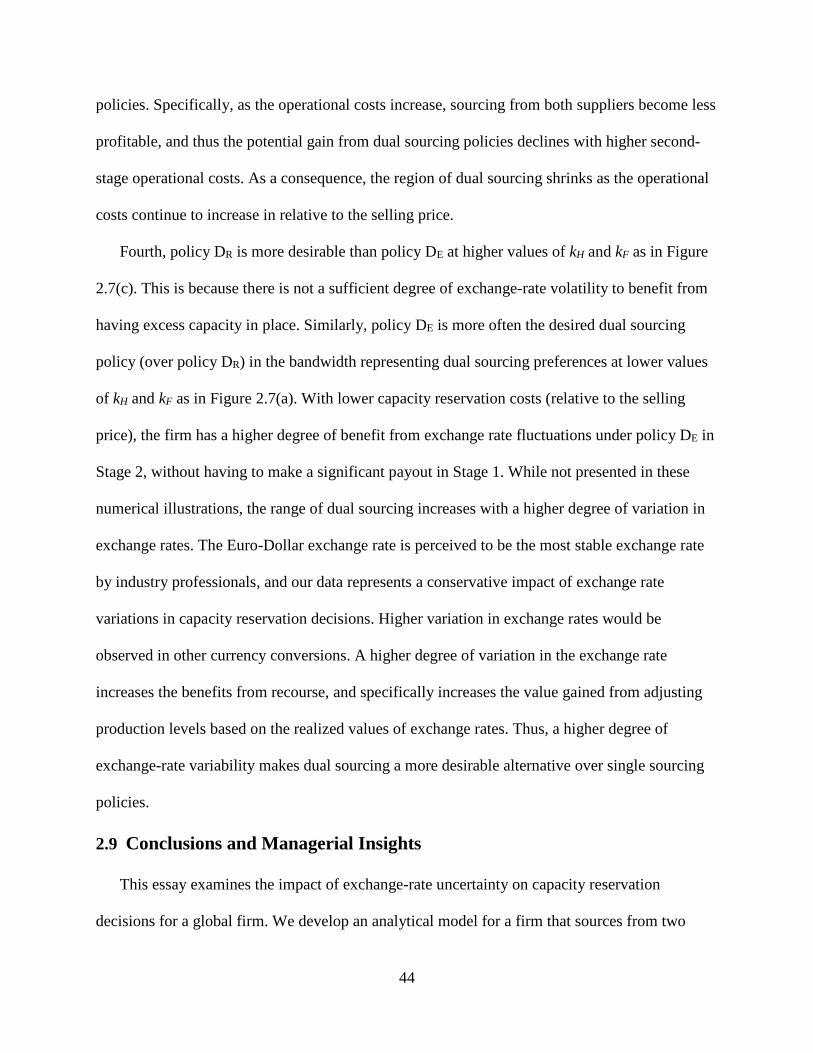
44

policies. Specifically, as the operational costs increase, sourcing from both suppliers become less

profitable, and thus the potential gain from dual sourcing policies declines with higher second-

stage operational costs. As a consequence, the region of dual sourcing shrinks as the operational

costs continue to increase in relative to the selling price.

Fourth, policy DR is more desirable than policy DE at higher values of kH and kF as in Figure

2.7(c). This is because there is not a sufficient degree of exchange-rate volatility to benefit from

having excess capacity in place. Similarly, policy DE is more often the desired dual sourcing

policy (over policy DR) in the bandwidth representing dual sourcing preferences at lower values

of kH and kF as in Figure 2.7(a). With lower capacity reservation costs (relative to the selling

price), the firm has a higher degree of benefit from exchange rate fluctuations under policy DE in

Stage 2, without having to make a significant payout in Stage 1. While not presented in these

numerical illustrations, the range of dual sourcing increases with a higher degree of variation in

exchange rates. The Euro-Dollar exchange rate is perceived to be the most stable exchange rate

by industry professionals, and our data represents a conservative impact of exchange rate

variations in capacity reservation decisions. Higher variation in exchange rates would be

observed in other currency conversions. A higher degree of variation in the exchange rate

increases the benefits from recourse, and specifically increases the value gained from adjusting

production levels based on the realized values of exchange rates. Thus, a higher degree of

exchange-rate variability makes dual sourcing a more desirable alternative over single sourcing

policies.

2.9 Conclusions and Managerial Insights

This essay examines the impact of exchange-rate uncertainty on capacity reservation

decisions for a global firm. We develop an analytical model for a firm that sources from two

45

suppliers, one domestic and one foreign, and sells in a single market. While demand uncertainty

in isolation (i.e., ignoring the impact of exchange-rate uncertainty) does not lead to dual sourcing

in our model, exchange-rate uncertainty creates the incentive for the firm to engage in dual

sourcing.

This study makes four contributions. First, we identify the set of potentially optimal policies

and the conditions that lead to these policies. Five potentially optimal sourcing policies emerge:

One onshore sourcing, two kinds of offshore souring policies, and two characteristically different

dual sourcing policies. One dual sourcing policy commits to a total capacity amount that would

equal the amount it would have reserved under the offshore sourcing policy, but it rations this

total capacity investment between the domestic and foreign suppliers according to the exchange-

rate uncertainty. This dual-sourcing policy can be perceived as a defensive and a conservative

approach as it is motivated to negate the detrimental consequences of an appreciating exchange

rate making the foreign supplier an expensive source. The same policy foregoes the benefits of a

lower cost foreign supplier under realizations of exchange-rate devaluation. The second dual

sourcing policy features excess capacity. The same amount of capacity is reserved at the foreign

supplier as with the offshore sourcing policy, and there is additional capacity reserved at the

domestic supplier. However, the amount of capacity reserved at the domestic supplier is less than

the amount that would have been reserved under the onshore sourcing policy. Thus, the domestic

supplier capacity is perceived as a backup capacity, and is intended to be utilized in order to

benefit from exchange-rate fluctuations. We show that these five policies can be located by

checking four optimality conditions. The conditions clarify how the firm switches its optimal

policy choice from one sourcing policy to another with increasing degrees of exchange-rate

volatility.

46

Second, our analysis shows that a lower sourcing cost is neither a necessity nor a sufficient

condition to reserve capacity at a supplier. Under exchange-rate uncertainty, lower unit sourcing

cost does not necessarily qualify a supplier as a potential source. It can be optimal to source only

from a foreign supplier that has a higher expected sourcing cost. This finding goes against the

common practice of low-cost sourcing and suggests that managers should think more deeply

about their sourcing policies under exchange-rate uncertainty. Moreover, our results show that

the firm may reserve capacity only at the foreign supplier even if the expected operational cost

(inclusive of production, transportation, duty, and localization expenses) is higher than the

selling price. This result makes our finding associated with reserving capacity only at the more

expensive supplier even more pronounced as it exemplifies the opportunity gains from the

currency fluctuations.

Third, we show that risk aversion makes dual sourcing more desirable. In particular, when

the firm’s optimal policy is offshore sourcing in the risk-neutral setting, the introduction of risk

aversion with a VaR requirement can trigger a policy switch to dual sourcing. Thus, under risk

aversion, dual sourcing becomes more pronounced over single sourcing.

Fourth, financial hedging can help eliminate the negative consequences of risk aversion and

enable the firm to replicate the expected profit of the risk-neutral policies. Thus, the firm obtains

the same set of five potentially optimal global sourcing policies in the presence of financial

hedging. As a consequence, our policy findings are robust as they continue to hold under risk

aversion and financial hedging.

In addition to the above four contributions, our study provides insights into the impact of

exchange-rate volatility on capacity reservation decisions. While the reserved capacity of the

foreign supplier increases with volatility, capacity reservation decisions at the domestic supplier

47

can exhibit both an increasing and decreasing behavior. The conditions for the increasing and

decreasing behavior are described under increasing exchange-rate uncertainty. Greater degrees of

exchange-rate volatility do not always increase domestic capacity and do not regularly lead to

higher flexibility. The firm may prefer to give up some of its allocation flexibility under policy

DE, for example, by reducing its domestic capacity and capitalizing more on the foreign capacity.

We have stated earlier that our work is motivated from the challenges faced by a specialty

furniture maker. Our work demonstrates numerically how our model applies to the products of

this firm. The firm’s prior sourcing decisions have ignored exchange-rate uncertainty, and have

relied on utilizing a single supplier which is selected based on the lower cost. Incorporating

exchange-rate uncertainty, our analysis shows that, when unit capacity reservation costs are

smaller relative to the selling price as in the case of book carts, the firm prefers dual sourcing

policies. When the unit capacity reservation cost is higher in comparison to the selling price as in

the case of office desks and chairs, then a single-sourcing policy is desired. The firm now

engages in dual sourcing for some of its products. We also report that both the rationing dual

sourcing policy and dual sourcing policy with excess capacity are currently being utilized among

the firm’s product portfolio.

48

CHAPTER 3: GLOBAL SOURCING UNDER YIELD UNCERTAINTY

3.1 Introduction

Coffee is one of the most popular beverages worldwide. The United States Department of

Agriculture, forecasts the global annual coffee consumption at a record of 150.8 million bags (60

kilograms, or approximately 132 pounds, per each bag) in its 2016/2017 forecast review1. While

the coffee consumption is expected to continue to experience a steady growth, the consumers

seem to increasingly demand high quality coffees around the world (Stabiner 2015, Craymer

2015). There are a few coffee roasters in the United States which have already targeted this

trending specialty coffee market, and are believed to be reshaping the coffee industry (Strand

2015). The pioneer coffee roasters in the specialty coffee industry are Intelligentsia, Stumptown,

and Counter Culture, which are called the Big Three of the Third-Wave Coffee, an initiative

aimed at enhancing the quality of the produced coffee. Third Wave Coffee is considered as a

specialty food product rather than a commodity. This is exemplified by the recent acquisitions of

Intelligentsia and Stumptown by Peet’s Coffee at high prices, indicating an increase in the

interest and practice in the specialty coffee market.

In order to be able to offer superior coffee, these leading coffee roasters rely heavily on direct

communication and close collaboration with the growers, which has given rise to a new form of

sourcing practices called Direct Trade. Through Direct Trade, specialty coffee roasters can

improve the quality of coffee beans by providing guidance and resources to the growers, and

closely monitoring the growth of coffee beans and the harvesting process. Direct Trade is

different from the traditional sourcing practice in the coffee industry which involves sourcing

through coffee traders and exchanges as described in Figure 3.1.

1 http://apps.fas.usda.gov/psdonline/circulars/coffee.pdf

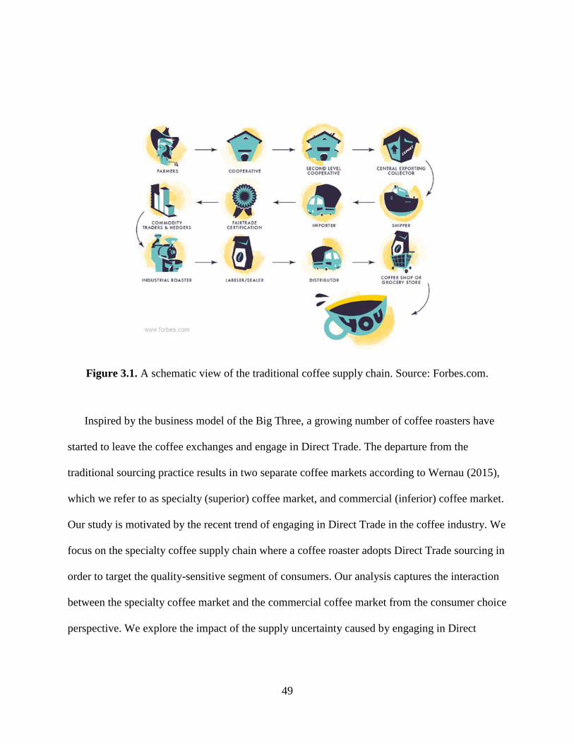
49

Figure 3.1. A schematic view of the traditional coffee supply chain. Source: Forbes.com.

Inspired by the business model of the Big Three, a growing number of coffee roasters have

started to leave the coffee exchanges and engage in Direct Trade. The departure from the

traditional sourcing practice results in two separate coffee markets according to Wernau (2015),

which we refer to as specialty (superior) coffee market, and commercial (inferior) coffee market.

Our study is motivated by the recent trend of engaging in Direct Trade in the coffee industry. We

focus on the specialty coffee supply chain where a coffee roaster adopts Direct Trade sourcing in

order to target the quality-sensitive segment of consumers. Our analysis captures the interaction

between the specialty coffee market and the commercial coffee market from the consumer choice

perspective. We explore the impact of the supply uncertainty caused by engaging in Direct

50

Trade, and the uncertainty in the global commercial coffee market on the coffee roaster’s

sourcing and pricing decisions.

We provide insights into managing a specialty-coffee supply chain, which is an emerging

phenomenon in the coffee industry, by addressing the following research questions:

1. What is the impact of yield uncertainty stemming from Direct Trade on sourcing

decisions of agribusinesses in a specialty coffee supply chain?

2. How does the uncertainty in the commercial coffee market influence the coffee roaster’s

level of investment in Direct Trade?

3. How should a coffee roaster set the price for its specialty product based on the market

price of the commercial coffee considering the consumer choice between the specialty

and the commercial coffees?

4. What is the impact of correlation between the specialty and the global commercial crop

supply?

Our study makes three contributions: First, to the best of our knowledge, our study is the first

to develop a mathematical model capturing the main driving forces that influence the sourcing

and pricing decisions in a specialty coffee supply chain. Incorporating the uncertainty in

commercial coffee market as well as the variation in the Direct Trade yield into our model, we

identify the optimal sourcing and pricing decisions of a specialty coffee roaster.

Second, we show that a conservative sourcing policy may emerge as an effective policy

under uncertainty, which would never be optimal in a deterministic setting. Our analysis

demonstrates that either yield uncertainty or the fluctuations in the price of the commercial

coffee may lead to a conservative sourcing policy where the coffee roaster intentionally

underinvests in Direct Trade. This sourcing policy—which we refer to as the “underinvestment”

51

policy—can be considered as an operational hedging approach that helps the coffee roaster

mitigate the negative consequences of the potential uncertainties. This result complements the

earlier literature on global production planning, which identifies “production hedging”

(deliberately producing less than demand) as an effective operational hedging policy (Kazaz et

al. 2005, Park et al. 2016) under exchange-rate uncertainty in manufacturing settings. Our work

shows a similar hedging approach for agribusinesses that operate under uncertainty pertaining to

crop yield and market-price of a competing inferior product. In our findings, the emerged

hedging policy can be interpreted as “capacity hedging” which involves underinvesting in

agricultural farmland. Under this conservative behavior, the firm utilizes its pricing lever in order

to shrink the market size at all realizations of the two random variables. Thus, the market size

served is smaller than what the firm would have served in the absence of a supply constraint.

Our third contribution relates with the impact of correlation between the specialty Direct

Trade supply and the global supply of commercial coffee beans. We observe that the specialty

crop supply would typically be negatively correlated with the market price of the commercial

coffee. Our analysis suggests that higher degrees of negative correlation between the two random

variables representing the specialty yield and the price of the commercial coffee improve the

expected profit, and therefore, the specialty coffee roaster benefits from investing in agricultural

regions where the specialty coffee yield becomes more strongly correlated with the global

commercial yield.

The remainder of this essay is organized as follows. Section 3.2 describes how our work

departs from the current literature. Section 3.3 introduces our model, Section 3.4 presents its

analysis; it identifies the optimal investment and pricing decisions, characterizes the

underinvestment policy, and examines the impact of uncertainty on Direct Trade investment

52

decisions. Section 3.5 provides concluding remarks. All proofs are relegated to the online

appendix.

3.2 Literature Review

This study examines the sourcing and pricing decisions of an agricultural firm under random

yield and market-price for a similar (and inferior) product. We begin our discussion with yield

and supply uncertainty. The supply chain management literature on sourcing strategies under

supply/yield uncertainty is extensive. Yano and Lee (1995) and Tang (2006) provide a

comprehensive review of the literature on managing yield/supply risk in manufacturing

environments. Our study is related with the stream of research in operations/supply chain

management literature which explores operational hedging strategies for managing supply

uncertainty. In this literature, supply diversification is proven to be an effective approach toward

mitigating supply risk. Gerchak and Parlar (1990), Parlar and Wang (1993), Anupindi and Akella

(1993), and more recently, Tomlin and Wang (2005), Dada et al. (2007), Burke et al. (2009), Jain

et al. (2014), and Tan et al. (2016) demonstrate the benefits of dual/multiple sourcing in

managing supply uncertainty. However, in these studies the firm (buyer) does not have pricing

power, and thus, the selling price is considered as exogenous. In addition, our work characterizes

an operational hedging policy that differs from supply diversification and involves underserving

the target market by lowering the level of investment in farmland capacity in the presence of

monopolistic power.

There are a few studies that consider a firm’s price-setting ability in the presence of supply

uncertainty. Li and Zheng (2006), and Feng (2010) investigate joint inventory and pricing

policies in multi-period manufacturing settings. Kazaz and Webster (2015) consider a single-

period Newsvendor model under supply and demand uncertainty and explore how the source of

53

uncertainty influence the tractability of the problem and the optimal decisions. Our study departs

from these papers by considering the consumer choice between two products and the effect of

uncertainty in the competing market on sourcing, production and pricing decisions of an

agricultural processor.

The most related body of research to our work includes studies that focus on agricultural

supply chains. Within this stream of research, a common sourcing framework is procuring

agricultural products through lease contracts (Kazaz 2004, Kazaz and Webster 2011) by which

an agricultural firm leases farmland at the beginning of the growing season and harvests the

realized crop yield at the end of the growing season. Our study uses a similar framework in

modeling sourcing decisions. However, it departs from the earlier studies. Kazaz (2004), Kazaz

and Webster (2011) examine the impact of yield-dependent trading cost on sourcing and

production planning of an agricultural firm which sells a single product. Our study, however,

considers two products—one superior and one inferior product— with two associated consumer

segments. Although our main focus is exploring the sourcing and pricing decisions of the

superior product, our analysis captures the consumer’s choice between the two products, which

affects the demand for the superior product.

Noparumpa et al. (2011) examine the interrelationships among downward substitution, price

setting, and fruit trading under supply and quality uncertainty. While we do not incorporate

quality uncertainty into our model, we capture the impact of uncertainty in the price of an

inferior product determined by the global market on sourcing and pricing of a superior product

by an agricultural processor.

Our model’s structure is similar to that of Noparumpa et al. (2015). Our study, however,

differs from their work in terms of the decisions, and the environmental factors influencing

54

sourcing and pricing decisions. They investigate a winemaker’s decisions on how to allocate a

single product between advance selling in the form of financial futures contract and retail

distribution. Our study, on the other hand, explores the impact of the interaction between two

different consumer segments on allocation decisions of an agricultural processor. Our study also

captures the farmland investment decisions made by the processor prior to the selling season and

incorporates the yield uncertainty stemming from such a sourcing practice.

There is a recent stream of literature that considers simultaneous sourcing of agricultural

inputs (Boyabatli et al. 2011, Boyabatli 2015). However, this body of research investigates

multi-product supply management where the crop yield is assumed to be deterministic using two

or more different agricultural inputs. Our study is structurally different from these papers as we

emphasize the effective policies for sourcing a single agricultural input under yield and market-

price uncertainty.

In sum, motivated by an emerging agribusiness practice in the coffee industry, our study

features a new agricultural supply chain framework. In order to target the fast-growing niche

segment of quality-sensitive consumers, a small number of coffee roasters have drastically

changed their sourcing policy and engaged in Direct Trade, which in turn has led to exposure to

supply risk. Our study investigates the sourcing and pricing decisions of such agricultural

processors and provides insights into managing the supply chain of the associated agricultural

products.

3.3 Model

In this section, we describe the problem and present the model developed to explore the

global sourcing decisions of a firm operating in an agricultural environment where yield

uncertainty influences the firm’s crop supply. The firm sells a finished product (i.e., roasted

55

coffee) which requires processing an agricultural product (i.e., coffee green beans) as input to be

converted to the final product. The main target market of the firm (processor) is the quality-

sensitive segment of consumers who prefer specialty coffees and are willing to pay a premium

price (hereafter “specialty segment”). The processor (coffee roaster) engages in Direct Trade

(DT) in order to be able to source quality coffee beans and offer superior processed (roasted)

coffee to the specialty segment. An inferior alternative for consumers is the Non-Direct-Trade

(NDT) roasted coffee which is extensively offered by a large number of coffee roasters, and is

desired by a massive population of consumers who consider coffee as a necessity product. As

such, we consider the NDT coffee as a commercial/commodity product whose price is

exogenously determined by the enormous global market.

We develop a two-stage stochastic model with recourse to examine the processor’s sourcing

and pricing decisions in the presence of yield uncertainty of the DT crop and price uncertainty of

the commercial coffee. The operating environment and the sequence of decisions can be

described as follows: Prior to the growing season, which corresponds to stage 1 of our model, the

processor engages in DT by going straight to the growers and leasing farmland, denoted Q.

Along with the leasing decision, the processor provides instructions to the growers in order to

ensure the desired quality of the specialty coffee crop. This initial investment costs l per unit of

farmland. At the end of the growing season, corresponding to stage 2 of our model, the processor

realizes (1) the DT crop yield to be processed and sold as a specialty coffee, and (2) the global

market price for the commercial coffee. The DT crop supply harvested at the end of the growing

season is expressed as Qy (stochastically proportional to the lease quantity) where y ∈ [yl, yh] is

the realization of a random variable Y with mean ȳ , standard deviation σy, probability density

function (pdf) g(y), and cumulative distribution function (cdf) G(y). The market (retail) price of

56

the commercial coffee, Φ, is considered random with realization φ ∈ [φl, φh], meanϕ , variance

σφ, pdf h(φ) and cdf H(φ). The uncertainty in the price of the commercial coffee represents the

uncertainty in the commercial market which stems from the fluctuations in the global yield of the

coffee beans and other uncertain economic factors. In our base model, the DT crop yield and the

price of the commercial coffee are considered as independent random variables, because the

amount of crop yield from DT is assumed to be relatively small compared to the amount of the

commodity coffee’s global yield, which implies negligible correlation between the two random

variables (Y, Φ). We later relax this assumption and analyze the impact of correlation on the

investment decision and the expected profit of the processor. We also assume throughout the

essay that the support of Y and Φ remain unchanged as the level of uncertainty associated with

each variable alters (except for the case of no uncertainty where the random variable is replaced

with its mean).

Upon the realizations of the DT yield and the market price of the commercial coffee, the

processor uses its monopolistic power within the specialty segment, and sets the selling price,

denoted p, for its offered specialty coffee targeted toward this segment. An equivalent

interpretation is that the processor determines the quantity of the specialty coffee to be sold,

denoted q, in this stage. The processing (roasting) cost is r per unit of product. The extra DT crop

is processed and salvaged at s where s ≥ r (i.e., the salvage value of the processed crop is higher

than the processing cost), and the shortage in the DT supply cannot be compensated by sourcing

from the spot market, as the offered coffee would not be considered a DT product. We note that

our conclusions do not depend on the inequality r ≤ s; if r > s, then the firm salvages prior to

processing with corresponding adjustment to relevant expressions, leading to no change in the

structure of the profit function. Figure 3.2 illustrates the sequence of decisions and realizations.

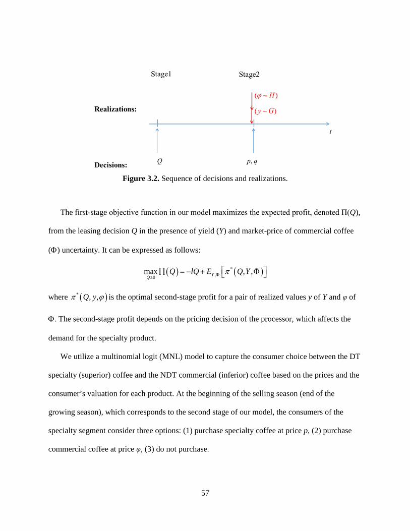
57

Figure 3.2. Sequence of decisions and realizations.

The first-stage objective function in our model maximizes the expected profit, denoted Π(Q),

from the leasing decision Q in the presence of yield (Y) and market-price of commercial coffee

(Φ) uncertainty. It can be expressed as follows:

( ) ( )*,0

max , ,YQQ lQ E Q YπΦ≥

∏ = − + Φ

where ( )* , ,Q yπ ϕ is the optimal second-stage profit for a pair of realized values y of Y and φ of

Φ. The second-stage profit depends on the pricing decision of the processor, which affects the

demand for the specialty product.

We utilize a multinomial logit (MNL) model to capture the consumer choice between the DT

specialty (superior) coffee and the NDT commercial (inferior) coffee based on the prices and the

consumer’s valuation for each product. At the beginning of the selling season (end of the

growing season), which corresponds to the second stage of our model, the consumers of the

specialty segment consider three options: (1) purchase specialty coffee at price p, (2) purchase

commercial coffee at price φ, (3) do not purchase.

58

The utility associated with each purchasing alternative is driven by the difference between

the valuation of the consumer for that particular product and the price of the product.

Specifically, the consumer’s valuation for the specialty coffee is Vs = vs + εs where εs is a random

variable with E[εs] = 0, and the consumer surplus – the difference between valuation and the

price – determines the random utility of purchasing the specialty product, i.e., Us = Vs − p = vs +

εs − p. The average utility of purchasing the specialty product among consumers is then us =

E[Us] = vs − p.

Similarly, the random utility of purchasing the commercial coffee can be expressed as Uc =

Vc − φ = vc + εc − φ, where εc is a random variable with E[εc] = 0. Thus, the average utility of

purchasing the commercial product is uc = E [Uc] = vc − φ. In order to reflect the preferences of

the specialty segment, we assume vs > vc.

Finally, the random utility of no-purchase option is U0 = ε0, which results in zero average

utility of this alternative among consumers, as ε0 is a random variable with E[ε0] = 0.

Among the three options, the consumers of the specialty segment choose the one associated

with the highest utility. Therefore, the probability of purchasing the specialty product is

[ ] [ ]0 0max{ , } max{ , }s c c s sP U U U P v pε ε ε> = − < −

Assuming that εs, εc, and ε0 are i.i.d. Gumbel random variables with zero mean and scale

parameter β, we note that max{εc, ε0}is a Gumbel random variable with E[max{εc, ε0}] = β ln 2,

and scale parameter β, and max{εc, ε0} − εs is a logistic random variable. As a result, the

probability of purchasing the specialty coffee is

[ ]( )/

0 ( )/ ( )/max{ , }1

s

c s

v p

s b v v peP U U U

e e

β

ϕ β β

−

− −> =+ +

59

which corresponds to the fraction of consumers in the specialty segment who purchase the

specialty coffee. Thus, the demand for the specialty coffee is determined by the MNL model as

follows:

[ ]( )/

0 ( )/ ( )/( | ) max{ , }1

s

c s

v p

s c v v peq p MP U U U M

e e

β

ϕ β βϕ−

− −= > =+ +

(3.1)

where M is the specialty segment size (i.e., the maximum consumer population who may

potentially buy the specialty product).

Consequently, the inverted demand function can be expressed as:

( | ) ln( )s

M qp q vk q

ϕ βϕ

−= +

(3.2)

where

( )/( ) 1 cvk e ϕ βϕ −= + (3.3)

The second-stage optimal profit can then be expressed as:

( ) ( )* , , , ,x |maq Qy

Q y q Q yπ ϕ ϕπ≤

=

where

( ) ( ) ( )

( )

| , ,

ln( )

|

s

q Q y s Qy q rQy

M qv s

p q q

q s r Qyk q

ϕ ϕ

βϕ

π = +

− −

−= − + +

−

(3.4)

is the second-stage profit function.

3.4 Analysis

3.4.1 Pricing and Processing Decisions

We begin our analysis by investigating the pricing and processing decisions of the firm after

realization of the DT crop yield and the market price for the commercial coffee (i.e., stage 2 of

60

our model). We determine the optimal price (p*(φ, y)) for the specialty DT product, which

provides the corresponding quantity to be sold (q*(φ, y)). These results utilize the Lambert W

function (Coreless et al. 1996). All proofs are relegated to the appendix.

Proposition 3.1. Let ( )

( )( )/ 1

( )/ 1

/ ( )( )

1 / ( )

s

s

v s

v s

W e k

W e k

β

β

ϕα ϕ

ϕ

− −

− −=

+, then

( )( )( )

* *

( )/ 1

ln , )( ), ,

1 / ( ) , )

if (( ), ( )

( if )(s

s

v s

M Qyv Qyk Qyy y

s W e

Qy M

M yk

p q

Q Mβ

α

α

β ϕϕϕ ϕ

β ϕ ϕ α ϕ− −

−+

+ +

<= ≥

,

and

( )( ) ( )

*

( )/ 1

if (

if

ln )( ), ,

/ ( ) ( )s

s

v s

M Qyv rk QyQ y

W e k s r

Qy Qy M

MQyM Qyβ

β ϕϕπ ϕ

β ϕ

α

α ϕ− −

−− + <

+ −

= ≥

.

The value of α(φ) is the optimal fraction of the specialty segment to be targeted by the

processor, and the value of Mα(φ) is the optimal market size to be served (optimal demand). We

observe that the processor sets different selling prices for the specialty coffee contingent upon

whether the crop supply (Qy) is sufficient for serving the optimal market size.

The next proposition shows how the optimal price of the specialty coffee (optimal “specialty

price”, hereafter) changes with the realized market price of the commercial coffee (realized

“commercial price”, hereafter). Throughout this essay, we use “increase”, “decrease”, and

“concave” in their weak sense.

Proposition 3.2. The optimal specialty price (p*(φ, y)) increases in the realized commercial

price (φ). However, the magnitude of the increase is less than that of φ, i.e., 0 < ∂p*(φ, y)/∂φ < 1.

61

The processor charges a higher specialty price at higher levels of realized commercial price.

We note that the demand for the specialty coffee depends on both the specialty price set by the

processor (p) and the realized commercial price determined by the global market (φ). Proposition

3.2 states that the optimal specialty price takes the same direction as the realized commercial

price. That is, if the commercial price increases (decreases), the specialty price should increase

(decrease) as well. Consequently, they have counter-balancing effects on the demand. The next

proposition identifies the dominant effect and clarifies how the optimal target market size

changes with respect to the realized commercial price.

Proposition 3.3. The optimal fraction of the specialty segment to be targeted by the processor

(α(φ)) and thus the optimal processing quantity (q*(φ, y)) increases in the realized commercial

price (φ).

Even though the processor raises the specialty price as commercial price increases, its effect

on the market allocation is dominated by the effect of commercial price. Consequently, the

optimal targeted fraction of the specialty segment expands if the realized commercial price

increases. This implies that the processor benefits from targeting a larger specialty market while

charging a higher price as the commercial coffee becomes more expensive.

3.4.2 Investment Decision

We next explore the processor’s investment decision at the beginning of the growing season

(i.e. Stage 1 of our model). From Proposition 3.1, we use the optimal second-stage profit

expressions to write the first-stage expected profit function as follows:

( ) ( )( )

( )/ 1

( )

ln ( ) ( )( )

( ) ( )( )

s

sU Q

v s

O Q

M Qyl ry Q Qy v g y h dydk Qy

eW sQy g y h dydk

Q

Mβ

β ϕ ϕϕ

β ϕ ϕϕ

− −

−∏ = − + + +

+ +

∫∫

∫∫ (3.5)

62

where ( ){ }( ) , | ( )U Q y Qy Mϕ α ϕ= < , and ( ){ }( ) , | ( )O Q y Qy Mϕ α ϕ= ≥ .

The following proposition indicates that there is always a unique optimal amount of farmland

to be leased for any given probability distributions of yield and commercial price.

Proposition 3.4. (a) The first-stage expected profit function Π(Q) is concave in the leasing

amount Q, and the optimal amount of farmland to lease, (denoted Q*, is the unique solution to

the below first order condition (FOC):

( ) ( )

ln ( ) ( ) ( ) ( )( )s

U Q O Q

M Qy My v g y h dyd syg y h dyd l ryk Qy M Qy

β β ϕ ϕ ϕ ϕϕ

−+ − + = + −

∫∫ ∫∫ (3.6)

(b) The optimal expected profit is

( )* *

( )/ 1*

*( )

*

( )

( ) ( ) ( ) ( )( )

sv s

U Q O Q

Q y eM g y h dyd W g y h yQ k

Q d dM y

β

β ϕ ϕ ϕ ϕϕ

− − ∏ = + −

∫∫ ∫∫ (3.7)

Note that the main objective of engaging in DT is to serve the quality-sensitive specialty

segment, because sourcing through DT allows the processor to ensure the desired quality by

providing instructions while closely collaborating with the growers. The growers, on the other

hand, have to have sufficient incentives to take part in DT. The processors typically pays the

farmer a premium price2 in order to ensure the availability of farmland in the long term. As a

result, sourcing through DT is costly for the processors, which creates a downward pressure on

the leasing decision and prevents the processor from overinvesting in DT. On the other hand, the

flexibility to charge a premium price for the specialty coffee segment creates an incentive to

increase investment in farmland associated with DT. The FOC (3.6) captures the tradeoff in these

opposing driving forces, and it helps determine the optimal leasing quantity. The two terms on

the left-hand side express the marginal revenue of leasing farmland when the crop supply falls

2 Intelligentsia Coffee website (http://www.intelligentsiacoffee.com/content/direct-trade)

63

short of the optimal target market (i.e., Qy ≤ Mα(φ)) and when there is sufficient supply (i.e., Qy

> Mα(φ)), respectively, while the right-hand side is the (expected) marginal cost of sourcing and

processing the crop supply of coffee beans.

Before proceeding with the optimal policy structure pertaining to the leasing decision of the

processor, we establish two benchmarks that serve beneficial in characterizing optimal behavior.

We begin with the first benchmark associated with the amount of farmland that would be leased

in the absence of uncertainty. It should be observed that when there is no uncertainty associated

with the DT crop supply nor with the commercial market, the processor invests in the exact

amount of farmland yielding the amount of supply that fulfills the optimal target market ( )Mα ϕ .

Our first benchmark, QD, establishes the lease amount of farmland for the processor that ignores

uncertainty by setting ( )Qy Mα ϕ= , and thus,

( ) /DQ M yα ϕ= .

We establish a second benchmark that helps characterize the processor’s potentially

conservative behavior. It should be observed that the lowest market size occurs when the

commercial price random variable takes its lowest value at the lower support of its pdf, φl. It

should also be observed that the highest crop yield for the processor is observed when the

random yield variable takes its highest value over the support of its pdf, yh. Our second

benchmark establishes the minimum amount of leased farmland that results in just sufficient crop

yield at its highest realization (yh) to cover the minimum market demand (equal to Mα(φl)). We

describe this benchmark as:

QT = Mα(φl) / yh.

Remark 3.1. QT < QD.

64

We note that, for Q < QT, the processor is guaranteed to operate under limited supply. This

can be seen from the fact that the maximum realized crop supply that can be attained at yh is less

than the minimum market demand at φl, i.e., Qyh < Mα(φl) for Q < QT. Thus, when Q < QT, the

firm operates under limited supply at all realizations of crop yield and market price uncertainty.

Next, we analyze the conditions leading to the conservative behavior as described above. We

then explore how the processor’s investment decision is affected by the variation in specialty

crop yield stemming from DT and the fluctuations in the price of the commercial coffee.

3.4.3 Underinvestment

In order to analyze the impact of uncertainties associated with the specialty crop supply and

the commercial price, we first identify an optimal sourcing policy under yield and commercial

price uncertainty, which would never be adopted if the yield and the commercial price were

deterministic. Specifically, under yield and commercial price uncertainty, our analysis shows that

the processor can deliberately underinvest in DT under certain conditions. We describe this

sourcing behavior as the “underinvestment” policy because the processor reduces the leasing

amount of farmland to the extent that it ensures at any realization of the yield and the

commercial price random variables, (1) it increases the selling price of the specialty coffee in

order to reduce the demand for specialty coffee and match the realized crop supply; and (2) it

serves a market demand that is smaller than what it would have served under an unconstrained

optimal price. In other words, by lowering the investment level below a threshold according to

the underinvestment policy, the processor chooses to always operate under supply shortage, and

it never fully utilizes the potential specialty coffee demand at the realized market-price φ, but

rather uses its pricing flexibility to reduce the market demand to match the realized crop supply.

65

It is worth noting that when there is no uncertainty associated with the DT crop supply or the

commercial market, the processor invests in the exact amount of farmland equal to QD, yielding

the amount of supply that fulfills the target specialty coffee demand that is equal to ( )Mα ϕ .

Therefore, the processor has no incentive to underinvest in DT when the supply and the

commercial market conditions are deterministic. Our analysis, however, shows that the

underinvestment policy can be optimal under either of yield and commercial price uncertainty.

In the global manufacturing network literature, Kazaz et al. (2005) are the first to introduce

an effective operational hedging policy –called “production hedging”—that involves producing

less than the total demand and thus underserving the markets. Park et al. (2016) build on this

work by showing that the production hedging policy is a viable risk mitigation approach. While

in both of these studies exchange-rate uncertainty is the main driver of underserving the markets,

our work indicates that yield uncertainty as well as price uncertainty in the competing market can

result in a similar operational policy in an agricultural environment. The underinvestment policy

explored in this essay can be considered as a “capacity hedging” policy where the low amount of

leased farmland proactively restricts the processing (production) quantity such that the firm

serves a market demand for specialty coffee that is strictly less than what it would have served

under an unconstrained optimal price, regardless of the realizations of yield and the commercial

price.

We first identify the condition that leads to underinvestment and then explore the impact of

the uncertainty associated with the specialty yield and the commercial market on the processor’s

investment policy.

Proposition 3.5. Let A represent the two-dimensional support of y and φ (i.e.,

( ){ }, | ,l h l hA y y y yϕ ϕ ϕ ϕ= ≤ ≤ ≤ ≤ ).

66

(a) It is optimal for the processor to underinvest in DT if and only if the below condition

holds

( )ln ( ) ( )( ) ( ) ( )h l h

sl h lA

y y yy v g y h dyd l ryk y y y

α ϕβ β ϕ ϕϕ α ϕ α ϕ

−+ − < + −

∫∫ (3.8)

(b) When it is optimal for the processor to underinvest, the optimal leasing quantity (QU*) is

the unique solution to the below FOC:

ln ( ) ( )( )s

A

M Qy My v g y h dyd yk Qy M Qy

l rβ β ϕ ϕϕ

−+ − = −

+∫∫ (3.9)

(c) The expected profit for the underinvestment policy can be expressed as:

( )*

** ( )

h

l

yU

U UUy

Q yQ M g y dyM Q y

β∏ =−∫ (3.10)

(d) The optimal amount of farmland under the underinvestment policy is less than the

minimum farmland space; specifically, QU* < QT.

Proposition 3.5 establishes the conditions under which the processor is better off by lowering

its investment level such that it ensures the specialty crop supply falls short of the optimal market

size to be targeted by the processor at any realizations of the yield and the commercial price.

Note that according to Proposition 3.3, the smallest portion of the specialty segment is targeted

by the processor when the commercial price is realized at its lowest level (φl). In addition, we

observe that when the processor faces supply shortage, it charges a market clearing price.

Condition (3.8) implies that the processor benefits from operating under supply shortage and

charging market clearing price than investing more on the DT when the marginal cost of

additional supply (right-hand side of the inequality) overweighs its expected marginal revenue

(left-hand side of the inequality) even when the highest possible realization of the DT supply

(Qyh) can barely fulfill the lowest possible level of optimal demand (i.e., Mα(φl)). Proposition

67

3.5(d), along with Remark 3.1, indicates that the optimal leasing quantity under underinvestment

policy is significantly lower than the optimal leasing quantity under deterministic setting.

Next, we examine the impact of yield and commercial price uncertainty on the investment

policy.

3.4.3.1 Impact of uncertainties on the investment policy and profit

In this section, we investigate how the investment policy is affected by the yield variation

and the commercial price fluctuations. We particularly study whether these uncertainties

encourage or hinder underinvestment policy, and whether their effects reinforce or

counterbalance the opposing forces in the optimal lease decision.

Proposition 3.6. (a) If for a given level of commercial price uncertainty (yield uncertainty), the

underinvestment policy is optimal under two-point distribution of random yield (random

commercial price), there exists a threshold for the degree of yield uncertainty (commercial price

uncertainty) above which underinvestment is optimal. (b) When the underinvestment policy

becomes optimal at a higher level of yield uncertainty (commercial price uncertainty), the

expected profit decreases compared to the case with lower levels of yield uncertainty

(commercial price uncertainty) where the underinvestment policy is not optimal.

The above proposition implies that both types of uncertainties faced by the processor leads to

the underinvestment policy becoming a more viable sourcing policy. Specifically, as long as the

underinvestment policy is optimal under the highest level of yield or commercial price variation

(under a two-point distribution), the processor eventually implements the underinvestment

policy. The firm continues to implement this policy as the variation increases. In addition, the

fact that underinvestment is associated with a lower expected profit suggests that this policy is

68

adopted under unfavorable circumstances caused by the uncertainty in yield and commercial

price.

We note that, under the underinvestment policy, the marginal revenue in the left-hand side of

(3.9) decreases as yield or commercial price variation increases. Consequently, at higher levels

of yield or commercial price uncertainty, the processor eventually restricts its DT investment

amount to such low levels that result in serving a specialty coffee demand that is strictly less than

what it would have served under an unconstrained optimal market demand. Essentially, the

underinvestment policy allows the processor to exercise its monopolistic power over the entire

specialty supply (by charging a market-clearing price) and at the same time save on the

opportunity cost of facing overage at higher investment levels, as the operating environment

becomes more uncertain.

Now that we observe the variation in the specialty yield as well as the uncertainty in the

commercial market encourage the adoption of the underinvestment policy, we investigate which

uncertainty is the main driver of this behavior. Are both yield and commercial price uncertainties

necessary for the underinvestment policy to become an effective sourcing policy? Can either of

these uncertainties by itself result in the underinvestment policy?

Proposition 3.7. Either yield uncertainty or commercial price uncertainty by itself can lead to

the underinvestment policy.

Our analysis demonstrates that either source of uncertainty in this operating environment can

cause the processor to adopt the underinvestment policy. In other words, neither yield nor

commercial price uncertainty can be considered necessary or the primary driver of the

underinvestment policy; they both contribute significantly to the optimality of this sourcing

policy.

69

The next proposition identifies how yield and commercial price uncertainty affects the DT

investment level of the processor when implementing the underinvestment policy.

Proposition 3.8. When the processor adopts the underinvestment policy, as the degree of yield

uncertainty or commercial price uncertainty increases, (a) the optimal leasing quantity

decreases, and (b) the expected profit decreases.

The above proposition, along with the findings in propositions 3.6 and 3.7, suggest that the

optimal leasing amount and the expected profit exhibit a diminishing behavior under an

increasingly uncertain operating environment. This is important because we note that when the

underinvestment policy is not optimal, the analytical investigation is inconclusive about the exact

behavior of the leasing quantity and the expected profit with respect to uncertainty. Propositions

3.6 and 3.7 imply that higher degrees of uncertainty eventually lead to the underinvestment

policy with lower levels of DT investment and expected profit. Proposition 3.8 complements

these findings by analytically showing that when the underinvestment policy is optimal,

additional uncertainty reduces the optimal amount of investment and the expected profit. We

can, therefore, conclude that the leasing quantity and the expected profit decreases in yield and

commercial price uncertainty from a general perspective.

Next, we relax the independence assumption between the two random variables describing

the yield and market price uncertainty, and explore the impact of correlation between the crop

supply obtained through DT and the price of the commercial coffee set by the global market.

3.4.3.2 Impact of correlation

It is potentially likely to have negative correlation between the specialty coffee (DT) yield

and the price of the commercial coffee. This is because the global yield of the commercial coffee

beans negatively impacts the commercial coffee price, and therefore, any (positive) correlation

70

between the specialty yield and the global yield results in a negative correlation between the

random yield and the random commercial price. In order to study the impact of correlation, we

compare two cases (in which the support for the two random variables Y and Φ remain

unchanged): (1) perfect correlation (denoted by the subscript “pc”) and (2) less-than-perfect

correlation (including independence; denoted by the subscript “lc”).

In case of perfect (negative) correlation, the commercial price is deterministically related

with the yield. Therefore, we consider the realization of the commercial price (φ) as a decreasing

function of the realization of DT yield (y) (i.e., φ(y) is a decreasing function of y) such that φ(yl)

= φh, and φ(yh) = φl. Consequently, the optimal fraction of the specialty segment to be targeted by

the processor (i.e., Mα(φ(y))) becomes a decreasing function of y. Therefore, for any given

leasing quantity (Q), there exists a threshold, denoted by ˆ( )y Q , for which we have:

ˆ( ( )) if ( )ˆ( ( )) if ( )

Qy M y y y QQy M y y y Q

α ϕα ϕ

< < ≥ ≥

The second-stage optimal profit can be expressed as in Proposition 3.1 (except for φ is

replaced with φ(y)), and we can write the first-stage expected profit function as follows:

( ) ( ) ( )

( )

ˆ ( )

( )/ 1

ˆ ( )

ln ( )( )

( )( )

l

h s

y Q

pc sy

y v s

y Q

M Qyl ry Q Qy v g y dyk y Qy

eW sQy g y dyk y

Q

Mβ

βϕ

βϕ

− −

−∏ = − + + +

+ +

∫

∫ (3.11)

In the case of less-than-perfect correlation, Φ(y) denotes the random commercial price with

E[Φ(y)] = φ(y) for a given realization of y. Accordingly, the first-stage expected profit function

can be expressed as:

71

( ) ( )( )

( )/ 1

( )

ln ( , )( )

( , )( )

lc

s

lc

lc sU Q

v s

O Q

M Qyl ry Q Qy v y dydk Q

Qy

eW sQy y dydMk

β

β ω ϕ ϕϕ

β ω ϕ ϕϕ

− −

−∏ = − + + +

+ +

∫∫

∫∫ (3.12)

where ( ){ }( ) , | ( )lcU Q y Qy Mϕ α ϕ= < , and ( ){ }( ) , | ( )lcO Q y Qy Mϕ α ϕ= ≥ when there is a less-

than-perfect correlation between y and φ, and ω(y,φ) is the joint distribution of Φ and Y.

The next proposition provides insights into how the correlation between the specialty yield

and the commercial price affects the sourcing policy.

Proposition 3.9. (a) If the underinvestment policy is optimal under perfect correlation, it is also

optimal under less-than-perfect correlation (including the case of independence between the two

random variables), and (b) When the underinvestment policy is optimal under all levels of

correlation, the expected profit is higher under the perfect correlation than that under less-than-

perfect correlation (including the case of independent random variables), for a given leasing

quantity.

This result implies that the underinvestment policy is less likely to be optimal under perfect

correlation than under less-than-perfect correlation. The finding suggests that the correlation

between the yield and the commercial price allows the processor to invest more freely in DT.

Recall that propositions 3.6, 3.7, and 3.8 imply that either type of uncertainties faced by the

processor is undesirable in this environment and negatively affects the processor’s expected

profit and the overall investment amount. Proposition 3.9 suggests that correlation mitigates the

adversarial effects of the variation in the specialty yield and the uncertainty in the commercial

market, and it improves the expected profit from a general perspective. We note that, as the

degree of negative correlation increases, the set of possible pairs of yield and commercial price

realizations shrinks, and thus, the operating environment becomes “less uncertain”. Therefore, it

72

is conceivable to infer that correlation raises the level of optimal investment and improves the

profit.

The consequence of this result is that it is beneficial for the coffee roasters to invest more in

the agricultural regions with the crop yield that is more strongly and positively correlated with

the global commercial coffee yield. It is well known that Brazil has the highest share of coffee

beans supply in the global market. Our analysis suggests that investing in agricultural regions

with strong correlation with Brazil’s coffee yield –as much as the geographical properties

necessary for high-quality coffee allows— is advantageous to the DT coffee roasters.

3.5 Conclusions and Managerial Insights

This essay examines sourcing and pricing decisions of an agricultural processor under yield

uncertainty of the agricultural input required for the offered specialty product and the price

uncertainty of the competing commercial product. Our study is motivated by a recent trend in the

coffee industry and makes several contributions.

First, we develop an analytical model which captures a trending supply chain framework

where Direct Trade is an emerging sourcing practice. In order to target the quality-sensitive

segment of consumers, a small number of coffee roasters have drastically changed their sourcing

policy and engaged in Direct Trade, which involves direct communication and close

collaboration with the growers, but results in increased exposure to crop supply risk. We identify

the optimal sourcing decision under yield and commercial price uncertainty in the first stage of

our proposed model, and the optimal pricing policy upon realizations of the specialty crop supply

and the commercial product’s price.

Second, we analyze the impact of yield and commercial price uncertainty, and demonstrate

that a viable sourcing policy—which would never be adopted in a deterministic setting—

73

emerges as a result of uncertainty. This policy requires the processor to deliberately underinvest

in farmland of the specialty segment by lowering the level of investment in Direct Trade. This

conservative sourcing policy highlights the significant impact of the variation in the specialty

yield as well as the uncertainty in the commercial market on the investment decisions of the

processor.

Third, our analysis indicates that the correlation between the specialty yield and the global

commercial yield improves the expected profit from a general perspective. Consequently, our

study suggests that the specialty coffee roaster benefits from investing in agricultural regions

where the yield is more strongly correlated with the global yield.

In sum, our study provides insights into managing a specialty-coffee supply chain which is

an emerging phenomenon in the coffee industry.

74

APPENDIX

Appendix to Chapter 2

Proposition 2A.1. The first-stage expected profit function for offshore sourcing is concave in

QF; (b) QF0 > 0.

Proof. (a) The objective function in (2.4) can be written as follows:

( ) ( )

( ) ( ) ( ) ( )

( ) ( ) ( )( ) ( ) ( )2

( )

0 0

(( ) )

0,

F

l F

oF F

H F F F F

Q

F F F F Fe Q

F F F F Fq eQ

E Q Q k u e Q

pD c e u e t Q p x Q f x dx g e de

pD c e u e t q e p x q e f x dx g e de

τ

τ

τ

∞

∞

Π = = − +

+ − − + − −

+ − − + + −

∫ ∫

∫ ∫

.

The first-order derivative of the profit function with respect to QF is:

( )( ) ( ) ( ) ( )

( )

)0,

1 (F

l

QH F

F F F F F FF e

E Q Qk u e c e u e t p F Q g e de

Q

τ ∂ Π = = − + + − − + + − ∂ ∫ .

Recall that τ(QF) = (p[1 – F(QF)] – tF)/(cF – uF) and observe that ∂τ(QF)/∂QF = – pf(QF)/(cF –

uF) ≤ 0. Substituting τ(QF) into the above first-order derivative provides the first-order (FOC)

condition in (2.9):

( )( ) ( ) ( )

( )

0,( ) ( )

F

l

QH F

F F F F FF e

E Q Qk u e c u Q e g e de

Q

τ

τ ∂ Π = = − + + − −

∂ ∫ .

Because ∂τ(QF)/∂QF ≤ 0, the second-order derivative is non-positive and the objective

function is concave in QF:

( )( ) ( )

)2

2

( ( )0,

l

FQH F

F FF Fe

FE Q Q

c u g e dd eQ Q

Qτ τ ∂ Π = = −∂ ∂∫ ≤ 0.

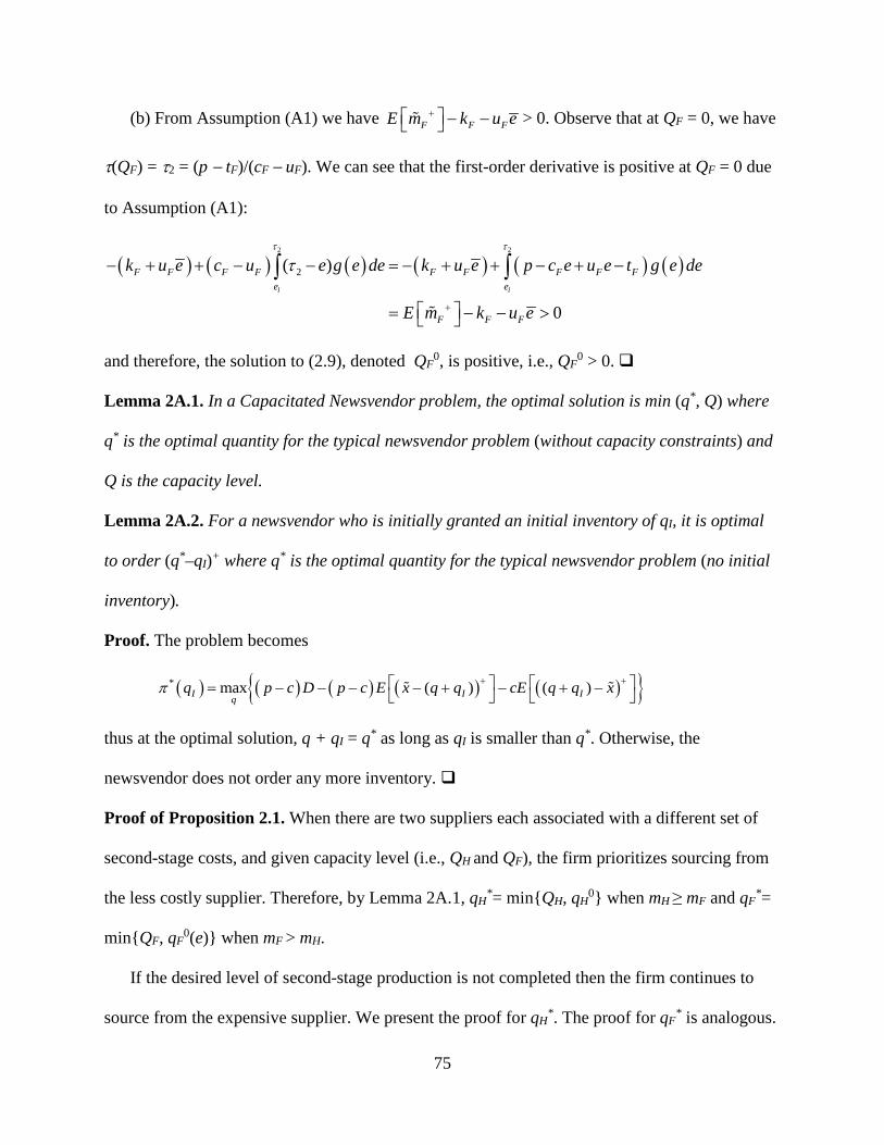
75

(b) From Assumption (A1) we have F F FE m k u e+ − − > 0. Observe that at QF = 0, we have

τ(QF) = τ2 = (p − tF)/(cF − uF). We can see that the first-order derivative is positive at QF = 0 due

to Assumption (A1):

( ) ( ) ( ) ( ) ( ) ( )2 2

2( )

0l l

F F FF F F F F Fe e

F F F

p c e u e tk u e c u e g e de k u e g e de

E m k u e

τ τ

τ

+

− + + − − = − + +

= − − >

− + −∫ ∫

and therefore, the solution to (2.9), denoted QF0, is positive, i.e., QF

0 > 0.

Lemma 2A.1. In a Capacitated Newsvendor problem, the optimal solution is min (q*, Q) where

q* is the optimal quantity for the typical newsvendor problem (without capacity constraints) and

Q is the capacity level.

Lemma 2A.2. For a newsvendor who is initially granted an initial inventory of qI, it is optimal

to order (q*–qI)+ where q* is the optimal quantity for the typical newsvendor problem (no initial

inventory).

Proof. The problem becomes

( ) ( ) ( ) ( ) ( ){ }* m ) )ax ( (I I Iqq p c D p c E x q q cE q q xπ + + = − − − − + − + −

thus at the optimal solution, q + qI = q* as long as qI is smaller than q*. Otherwise, the

newsvendor does not order any more inventory.

Proof of Proposition 2.1. When there are two suppliers each associated with a different set of

second-stage costs, and given capacity level (i.e., QH and QF), the firm prioritizes sourcing from

the less costly supplier. Therefore, by Lemma 2A.1, qH*= min{QH, qH

0} when mH ≥ mF and qF*=

min{QF, qF0(e)} when mF > mH.

If the desired level of second-stage production is not completed then the firm continues to

source from the expensive supplier. We present the proof for qH*. The proof for qF

* is analogous.

76

When mF > mH, if the foreign supplier is in short of capacity (i.e., min{QF, qF0(e)} = QF )),

we know from Lemma 2A.2 that the domestic source can still be utilized as long as qH0 > QF =

qF*. In this case, the optimal production quantity would be (qH

0 – QF )+ if there were no capacity

constraints. It follows that qH* = min{QH , (qH

0 – QF)+} when QH restricts the production quantity.

Proposition 2A.2. The first-stage expected profit function in region R1 is jointly concave in (QH,

QF).

Proof. The profit function in region R1 can be expressed as follows:

( ) ( ) ( )( ) ( )

( ) ( ) ( )

( ) ( )

( ) ( ) ( )

( )

1

1

( )

( )

( )

, 1

H F

H F

l

H F

H

H F

e

Q

H F H H H F F F

H H H H F F F F

H FQ Q

H H H H F F F F

H FQ Q

H H H

Q

Q

Q Q

H

F

E Q Q R k u Q k u e Q

pD c u t Q c e u e t Q

g e dep x Q Q f x dx

pD c u t Q c e u e t Q

g e dep x Q Q f x dx

pD c u t Q

c

τ

τ

τ

τ

τ

∞

+

+

∞

+

+

Π = − + − + − − + − − +

+ − −

− − + − − +

+ − −

− − +

+ −

−

−

∫ ∫

∫ ∫

∫ ( )( )

( ) ( )

( )

( ) ( ) ( ) ( )

0

0

0

( )

( )

( )

( )

H

F

h

H

F F F H

Fq

e

H H H H HQ

e

Q

e u e t q Q g e de

p x q f x dx

pD c u t Q p x Q f x dx g e de

e

e

τ

∞

∞

− + − − −

+ − − + − −

∫

∫ ∫

(A.1)

The first- and second-order derivatives of the profit function with respect to the capacity

decisions are

( )( ) ( ) ( ) ( )

( ), 1( )

H F

l

Q QH F

F F F F H FF e

E Q Q Rk u e c u Q Q e g e de

Q

τ

τ+ ∂ Π = − + + − + −

∂ ∫

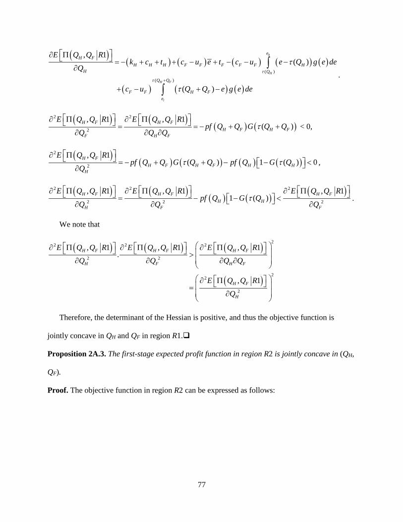
77

( )( ) ( ) ( ) ( ) ( )

( ) ( ) ( )

( )

( )

, 1( )

( )

h

H

H F

l

eH F

H H H F F F F HH Q

Q Q

F F H Fe

F

E Q Q Rk c t c u c u e Q g e de

Q

c u Q Q e g e

e

de

tτ

τ

τ

τ+

∂ Π = − + + + − − − −∂

+ − + −

+ ∫

∫.

( ) ( )( ) ( )

2 2

2

, 1 , 1( )H F H F

H F H FF H F

E Q Q R E Q Q Rpf Q Q G Q Q

Q Q Qτ

∂ Π ∂ Π = = − + +∂ ∂ ∂

< 0,

( )( ) ( ) ( ) ( )

2

2

, 1( ) 1 ( ) 0H F

H F H F H HH

E Q Q Rpf Q Q G Q Q pf Q G Q

Qτ τ

∂ Π = − + + − − < ∂,

( ) ( )( ) ( )

( )2 2 2

2 2 2

, 1 , 1 , 11 ( )H F H F H F

FH

FH

H

E Q Q R E Q Q R E Q Q Rpf Q G Q

Q Q Qτ

∂ Π ∂ Π ∂ Π = − − < ∂ ∂ ∂.

We note that

( ) ( ) ( )

( )

22 2 2

2 2

22

2

, 1 , 1 , 1.

, 1

H F H F H F

H H F

H F

H

F

E Q Q R E Q Q R E Q Q R

Q Q Q Q

E Q Q R

Q

∂ Π ∂ Π ∂ Π >∂ ∂ ∂ ∂

∂ Π =∂

Therefore, the determinant of the Hessian is positive, and thus the objective function is

jointly concave in QH and QF in region R1.

Proposition 2A.3. The first-stage expected profit function in region R2 is jointly concave in (QH,

QF).

Proof. The objective function in region R2 can be expressed as follows:

78

( ) ( ) ( )

( )( )

( ) ( ) ( )( )

( ) ( )( )

( ) ( )( )

( )

1

01

0

0

0( )

0

( )

( )

( )

( )

, 2

lo

F

H

H

H

h

H F H H H F F F

H F

e F F F F Hq

H F F F F H

Fq

H H H

H H HQ

e

H H H

e

Q

E Q Q R k u Q k u e Q

pD q Q

g e dec e u e t

c u t

Q p x q f x dx

pD Q c e u e t q Q

g e

c u t e

dep x q fe

c u

x d

pD t

x

Q

τ

τ

τ

τ

∞

∞

Π = − + − + − −

+ − − + −

− − − + −

+ − −

+ −

− +

−

− +

− +

∫ ∫

∫ ∫

∫ ( ) ( ) ( )H

H HQ

p x Q f x dx g e de∞

− −

∫

(A.2)

The first- and second-order derivatives of the profit function with respect to QH are

( )( ) ( ) ( ) ( )

( ) ( ) ( ) ( )

1

( )

( )

, 2

H

h

H

QH F

H H H H H F F FH

e

H H H F F H FQ

E Q Q Rk u c u t c e u e t g e de

Q

c u t c u Q t g e de

τ

τ

τ

τ

∂ Π = − + + − − + + − + ∂

+ − − + + − +

∫

∫

( )( ) ( )

( ) ( ) ( ) ( )2

2( )

, 21 ( ) 0.

h

H

eH F H

F F H HH F FQ

E Q Q R pf Qc u g e de pf Q G Q

Q c uτ

τ ∂ Π − = − = − − < ∂ −

∫

Therefore, the objective function is concave in QH. We next show that the objective function

is linear in QF. We have

( )( ) ( )

, 2H FF F F H

F

E Q Q Rk u e E m m

Q++

∂ Π+ = − + − ∂

(A.3)

which is constant and independent of QF and QH implying that

( ) ( )2 2

2

, 2 , 2H F H F

F H F

E Q Q R E Q Q R

Q Q Q

∂ Π ∂ Π =∂ ∂ ∂

= 0.

The determinant of the Hessian for the objective function in R2 is 0, and thus the profit function

is jointly concave in QH and QF in region R2.

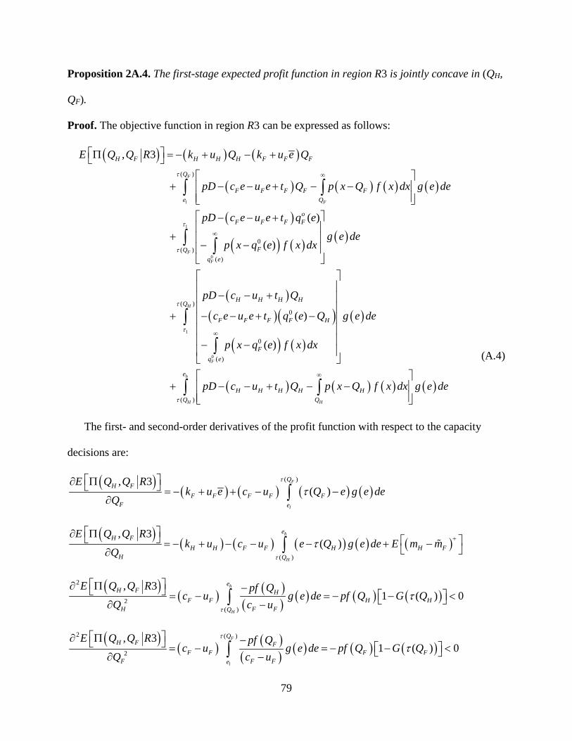
79

Proposition 2A.4. The first-stage expected profit function in region R3 is jointly concave in (QH,

QF).

Proof. The objective function in region R3 can be expressed as follows:

( ) ( ) ( )

( ) ( ) ( ) ( )

( )

( ) ( ) ( )

( )( )( )

0

1

0

1

( )

0( )

( )

( )0

( )

( )

( )

, 3

( )

F

H

l F

F

F

F

H F H H H F F F

F F F F Fe Q

oF F F F

Fq

H

F F F F H

q

Q

Qe

H H HQ

e

E Q Q R k u Q k u e Q

pD c e u e t Q p x Q f x dx g e de

p e

e

c

D c e u e t q

g e dep x q f x dx

pD Q

c e u e t q Q

p

u

q

e

x

t

τ

τ

τ

τ

τ

∞

∞

∞

Π = − + − +

+ − − + − − − − +

+ − −

− +

−

+ − − + −

− −

∫ ∫

∫ ∫

∫

∫ ( ) ( )

( )

( ) ( ) ( ) ( )

0

( )

( )

h

HH

H H

F

HQ

HQ

e

H

g e de

f x dx

pD Q p x Q f x dx g e d

e

c eu tτ

∞

+ − − −

− +∫ ∫

(A.4)

The first- and second-order derivatives of the profit function with respect to the capacity

decisions are:

( )( ) ( ) ( ) ( )

( ), 3( )

l

FQH F

F F F F FF e

E Q Q Rk u e c u Q e g e de

Q

τ

τ ∂ Π = − + + − −

∂ ∫

( )( ) ( ) ( ) ( ) ( )

( )

, 3( )

h

H

eH F

H H F F H H FH Q

E Q Q Rk u c u e Q g e de E m m

Q τ

τ + ∂ Π = − + − − − + − ∂ ∫

( )( ) ( )

( ) ( ) ( ) ( )2

2( )

, 31 ( ) 0

h

H

eH F H

F F H HH F FQ

E Q Q R pf Qc u g e de pf Q G Q

Q c uτ

τ ∂ Π − = − = − − < ∂ −∫

( )( ) ( )

( ) ( ) ( ) ( )2 ( )

2

, 31 ( ) 0

F

l

QH F F

F F F FF F Fe

E Q Q R pf Qc u g e de pf Q G Q

Q c u

τ

τ ∂ Π − = − = − − < ∂ −∫

80

( )2 , 30 H F

H F

E Q Q R

Q Q

∂ Π =∂ ∂

.

We note that the determinant of the Hessian is positive, leading to joint concavity in region

R3.

Lemma 2A.3. The objective function (2.4) is continuous.

Proof. Note that

( ) ( ) ( ) ( )

( )( ) ( )

( ) ( )( )

( ) ( )( )

( )

0 0

1

0

10 ( )

( ) ( )

0

0

0( )

0

lim , li

( )

( )

m , 1H F H H F H

l

H

H

F

H F H F H H H F F FQ Q q Q Q q

H H H H F F F F F

e Hq

H H H H F F F F HQ

Fq e

E Q Q E Q Q R k u Q k u e Q

pD c u t q Q c e u e t Q

g e dep x q f x dx

pD c u t Q ec

e

e u e t q Q

p x q

τ

τ

τ

−+ → + →

∞

∞

Π = Π = − + − +

− − + − − − +

+

− −

− − + − − + −

+− −

∫ ∫

∫ ∫ ( )( )

( ) ( ) ( ) ( )( )

h

H H

e

H H H H HQ Q

g e def x dx

pD c u t Q p x Q f x dx g e deτ

∞

+ − − + − −

∫ ∫

where by definition, τ (QH + QF = qH0) = τ1. This expression is equal to

( ) ( ) ( )0 00( ), 2 | lim , , |

H F H H F HH F HH F H F H FQ Q q Q Q qQ Q q

E Q Q R E Q Q E Q Q++ = + =+ →

Π = Π = Π

where the first equality holds by definition. Hence, the objective function is continuous along the

boundary line of QH + QF = qH0.

Similarly, along the boundary QF = qH0,

81

( ) ( ) ( ) ( )

( ) ( ) ( ) ( )

( ) ( )( )

( ) ( )( )

0 0

1

0

10

0

0

( )

( )

( )

0

0

0

lim , lim ,

( )

( )

3F H F H

l

H

H

H

F

H F H F H H H F F HQ q Q q

F F F H Hq

H F F F F H

e

H H

e

q

H

e

Q

F

Q

E Q Q E Q Q R k u Q k u e q

pD c e u e t q p x q f x dx g e de

pD Q c e u e t q Q

g e dep

c u t e

ex q f x dx

τ

τ

τ

τ

+→ →

∞

∞

Π = Π = − + − +

+ − − + − −

− − − + −

+ − −

+

− +

∫ ∫

∫ ∫

( ) ( ) ( ) ( )H

h

H H HH HQ

pD Q p x Q f x dxt g e dec u∞

− − −

− +∫ ∫

where by definition, τ (QF = qH0) = τ1. This expression is equal to

( ) ( ) ( )0 0 0, 2 | lim , , |

F H F HF HH F H F H FQ q Q qQ q

E Q Q R E Q Q E Q Q+= =→

Π = Π = Π

which implies that the objective function is continuous along this boundary line as well. As a

result, the objective function is continuous everywhere.

Lemma 2A.4. The profit function (2.4) is differentiable.

Proof. Along the boundary line of QH + QF = qH0, the left derivative of the objective function

with respect to QF is

( )( ) ( ) ( ) ( )

( ) ( ) ( ) ( )

( ) ( )

1

0

1

0

1( )

, 1lim

, 2 , 2|

H F Hl

l

H F H

H FF F F FQ Q q

F e

F F H H H F F Fe

H F H F

Q Q qF F

E Q Q Rk u e c u e g e de

Q

k u e c u t c e u e t g e de

E Q Q R E Q Q R

Q Q

τ

τ

τ−+ →

+ =

∂ Π = − + + − −∂

= − + + − + − − +

∂ Π ∂ Π = =∂ ∂

∫

∫

where the last expression is the right derivative of objective function along the same boundary

line.

The left derivative of the objective function with respect to QH is

82

( )( ) ( )

( ) ( ) ( ) ( ) ( ) ( )

0

1

( )

1( )

, 1lim

( )

H F H

h

H l

H FH H H F F FQ Q q

He

F F H F FQ e

E Q Q Rk c t c u e t

Q

c u e Q g e de c u e g e deτ

τ

τ τ

−+ →

∂ Π = − + + + − +∂

− − − + − −∫ ∫.

By rearranging the terms, we can rewrite the above derivative as follows:

( )( ) ( ) ( ) ( )

( ) ( ) ( )

( )

0

1

0

( )

( )

(

, 1

,|

)

|

2

H

H H

H F H

H

F

h

Q

e

H F

H FH H H H H F F FQ Q q

H

H H H F F

H F

Q Q qH

Q

E Q Q Rk u c u t c e u e t g e d

t

eQ

c u t c u g e de

E Q Q R

Q

Q t

τ

τ

τ

+ =

+ =

∂ Π = − + + − − + + − + ∂

+ − − + + −

∂ Π =∂

+

∫

∫

By definition, the above derivative is equal to the right derivative of the objective function

along the same boundary line. Thus, the objective function is differentiable along the boundary

line of QH + QF = qH0.

Along the boundary line of QF = qH0, the right derivative of the objective function with

respect to QF is

( ) ( )

( ) ( ) ( ) ( )

( ) ( ) ( ) ( )

( )

00

1

1

0

1

, 3,lim |

, 2|

F H

l

F H

F H

l

H FH FQ qQ q

F F

F F F F

F F H H H F F F

H F

Q qF

e

e

E Q Q RE Q QQ Q

k u e c u e g e de

k u e c u t c e u e t g e de

E Q Q R

Q

τ

τ

τ

+ =→

=

∂ Π ∂ Π =∂ ∂

= − + + − −

= − + + − + − − +

∂ Π =∂

∫

∫

where the last term is the left derivative of objective function along the same boundary line.

83

The right derivative of the profit function with respect to QH is

( )( ) ( ) ( ) ( )

( ) ( ) ( )

( ) ( ) ( ) ( )

( ) ( ) ( )

( )

0

1

1

0

( )

( )

( )

1

( )

1( )

, 3lim

, 2|

( )

F H

F

H

H

h

H

h

H

H

H FH H F FQ q

Q

e

HQ

Q

H H H

e

H H H H F

H

F F

H H F F F

F F

Q

Q

H F

qH

E Q Q Rk u c u e g e de

Q

c u g e de

k u c e u e t g e de

c u g

Q

c u t

c u t Q e de

E Q R

Q

t

Q

τ

τ

τ

τ

τ

τ

τ

τ τ

τ

+→

=

−

∂ Π = − + + − −∂

+ − −

= +

− + +

− + + − + − +

+ − + −

∂ Π =∂

∫

∫

∫

∫

By definition, the last expression is the left derivative of the objective function along that

same boundary line. Therefore, the objective function is differentiable along the boundary line of

QF = qH0 as well. In sum, the objective function is differentiable everywhere.

Lemma 2A.5. Onshore sourcing (H) is the optimal policy if and only if QF0 < QH

0.

Proof. From Proposition 2A.2, we observe that in R1 the shadow price of QH monotonically

decreases in QH as long as the total capacity is fixed. Note that this shadow price is positive at

solution (QH = QF0, QF = 0) due to concavity of the profit function in QH. Moreover, the shadow

price of QF in R1 remains the same as long as the total capacity is unchanged. Therefore, the

solution (QH = QF0, QF = 0) dominates all solutions along the line QH + QF = QF

0. However, this

dominant solution corresponds to onshore sourcing which itself is dominated by the optimal

onshore sourcing policy H (QH*= QH

0, QF*= QF

0).

Consequently, below the line QH + QF = QH0, the optimal solution is the onshore sourcing

policy H.

84

Proof of Proposition 2.2. From differentiability (lemmas 2A.3 and 2A.4) and piecewise

concavity of the objective function (propositions 2A.2, 2A.3, and 2A.4), it follows that the

objective function is jointly concave in QH and QF everywhere.

Proof of Proposition 2.3. The first derivative of the objective function in R2 with respect to QF

is given in (A.3) as follows:

( )( ) ( )

, 2H FF F F H

F

E Q Q Rk u e E m m

Q++

∂ Π+ = − + − ∂

.

The above derivative is constant and is independent of QF and QH. Therefore, the objective

function in region R2 is linear in QF, which implies that there is no interior solution in this

region.

Proof of Proposition 2.4. We have already shown that the objective function in (2.4) is jointly

concave in QH and QF, and that there is no interior solution in region R2 where the shadow price

of QF is constant (independent of QH and QF). Therefore, the sign of this shadow price given in

equation (A.3) leads us to the region where the optimal solution is located. If it is positive

(negative), the optimal solution lies in region R3 (region R1) and that the optimal solution is an

interior solution if the solution to system of equations in (2.13)(system of equations in (2.11))

exists. Suppose the shadow price in (A.3) is positive, i.e.,

( ) 0F H F FE m m k u e++ − − − >

(A.5)

The proof for parts (c) and (e) of the proposition requires analyzing region R3.

Region R3: In this region, it can observed from (2.13) that the second equation (first-order

condition for QF) is a rearrangement of equation (2.9), and results in the same optimal solution

QF0.

85

In order for QH* to be positive, we must have

( )0

, 3|

H

H FQ

H

E Q Q R

Q =

∂ Π ∂

as positive. It is

shown in the proof of Proposition 2A.4 that this derivative does not depend on the value of QF.

Hence,

( )( ) ( ) ( ) ( )

2

2 1

0

, 3|

h

H

H FQ H H H H F

H

eE Q Q Rk u m g e de m m g e de

Q

τ

τ τ=

∂ Π = − + + + −∂ ∫ ∫

must be positive, implying that

( ) ( )0

, 30|

H

H FQ H F H H

H

E Q Q RE m m k u

Q+

=

+ ∂ Π = − − − ∂> . (A.6)

Therefore, ( )H F H HE m m k u+ + − − − must be positive for DE to be optimal. Otherwise, the first-

order derivative with respect to QH is negative and QH* = 0, which results in the offshore

sourcing policy FH.

On the other hand, defining τ'= τ (QH + QF = QH0) = (cH + tH + kH – tF )/(cF – uF), we have

( ) ( ) ( )0

,|

H H

H FF H F HQ Q

H

E Q QE m m E m M

Q+ ++

=+

∂ Π = − − − ∂ < 0. (A.7)

As a result, QH* is lower than QH

0 in this region.

For parts (a), (b) and (d) of this proposition, we investigate Region R1.

Note that OC2 is identical to inequality (A.5). Therefore, if OC2 does not hold (i.e., the first-

order derivative of the objective function in (A.2) with respect to QF in region R2 is negative),

the optimal solution must lie in region R1.

Region R1: In this region we can observe from the system of equations in (2.11) that the

solution to the second equation (corresponding to the first-order condition for QF), i.e.,τHF*, is

86

identical to the solution in equation (2.9) , i.e., τF*. Therefore, an interior optimal solution must

satisfy

* * 0H F FQ Q Q+ = (A.8)

From (A.8), we have( )

( )0

, 1 | 0

H F F

H F

Q Q QF

E Q Q R

Q + =

∂ Π =∂

at the optimal solution. In order for

QH* to be positive, we need

( )00,

, 1|

H F F

H F

Q Q QH

E Q Q R

Q = =

∂ Π ∂

to be positive. We have

( ) ( ) ( )

( )

0 00, 0,

, 1 , 1 , 1| |

H F F H F F

H F H F H F

Q Q Q Q Q QH H F

H H H F F F

E Q Q R E Q Q R E Q Q R

Q Q Q

m k u E m k u e

= = = =

+

∂ Π ∂ Π ∂ Π = −∂ ∂ ∂

= − − − − −

. (A.9)

Thus, ( )H H H F F Fm k u E m k u e+ − − − − − must be positive for DR to be optimal. Otherwise,

QH* = 0 corresponding to the offshore sourcing policy FL.

On the other hand, from Lemma 2A.5, in order for QF* to be positive, QF

0 > QH0 must hold.

Equivalently, the derivative of the objective function in (A.1) with respect to QF along the line

QH + QF = QH0 (i.e.,

( )0

, 1|

H F H

H F

Q Q QF

E Q Q R

Q + =

∂ Π ∂

) must be positive. We have

( ) ( )0

, 1|

H F H

H FF H F FQ Q Q

F

E Q Q RE m M k u e

Q++

+ =

∂ Π = − − − ∂ . (A.10)

Hence, ( )F H F FE m M k u e++ − − −

must also be positive for DR to be optimal. Otherwise,

QF* = 0 corresponding to the onshore sourcing policy H.

87

Furthermore, as ( )[ ]

0 , 0

,| 0

H H F

H F

Q Q QH

E Q QQ = =

∂ Π

∂= by definition, and ( )[ ]2 ,

0H F

H F

E Q QQ Q

∂ Π<

∂ ∂, we have

( )[ ]0 , 0

,| 0

H H F

H F

Q Q QH

E Q QQ = >

∂ Π<

∂, which implies that QH

* must be lower than QH0 in region R1.

The Special Case of Low Volatility in Exchange Rate and/or High Profit Margin:

This is the special case where the volatility in exchange rate is so low, or the profit margin is

so high, that mF > 0 for all exchange-rate realizations in the second stage (i.e., τ2 > eh in Figure

2.3). First, the set of potentially optimal solutions remains the same. This is because the expected

profit function in the first stage does not depend on τ2 in any of the regions. Consequently, the

system of equations in (2.11) and (2.13) remain the same, which results in the same set of

potentially optimal solutions. Second, the optimality conditions also remain the same. The reason

is as follows: First, inequality (A.5) is independent of τ2. Second, in the derivations of equations

(A.6), (A.7), (A.9) and (A.10), τ2 is replaced with eh, which causes Fm+ to be replaced with Fm .

Therefore, if mF is always positive, then we can simplify all of the optimality conditions by

replacing Fm+ with Fm . However, keeping Fm+ leads to the general conditions.

Therefore, the set of potentially optimal solutions and the optimality conditions are robust to

the magnitude of exchange-rate volatility and to the variation in profit margin.

Proof of Proposition 2.5. Note that the first-order derivative of the objective function in an

offshore sourcing policy with respect to QF evaluated at qH0 is equal to the derivative of the

global sourcing objective function with respect to QF evaluated at the same point. i.e.,

( )[ ] ( )[ ] ( )0 0

,| |

0,F H F H

H F H F

Q q Q qF F

F H F F

E Q Q E Q QQ Q

E m m k u e= =

++∂ Π ∂ Π

∂ ∂

= − − − = =

88

Hence, QF0 > qH

0 is equivalent to the optimal global sourcing policy being in region R3, and

QF0 < qH

0 is equivalent to the optimal global sourcing policy being in region R1. Moreover, for

part (b), QF0 > QH

0 ensures that the optimal policy is not H.

Proof of Proposition 2.6. If kF + cF ē + tF < kH + cH + tH, then p – cF ē – tF – kF > p – cH – tH –

kH , which means [ ] F H HF F HE m u ek km u> −−− − . This has two implications: First, the

opposite of OC3 holds (i.e., F F F H H HE m k u e m k u+ − − > − − ), which in turn implies DR is

never optimal in this case. Second, OC1 holds because

( ) ( ) [ ] ( )F H F H F H H H F HH FH FE m M E k k um M E m m k u E m m u e+ +++ − ≥ − = − − − > − − − > +

Therefore, from Table 2.1, if OC2 does not hold, then FL is the optimal policy. Otherwise, if

OC2 holds but OC4 does not hold, then FH is the optimal policy. Finally, if both OC2 and OC4

hold, then DE is the optimal policy.

Proof of Proposition 2.7. The inequality kF + cF ē + tF ≥ kH + cH + tH by itself does not imply

that the optimality conditions hold or not. If OC2 holds and OC4 does not hold, the optimal

policy is FH. Moreover, if OC2 and OC3 do not hold and OC1 holds, the optimal policy is FL.

Proof of Proposition 2.8. The inequality p – (cF – uF) ē – tF < 0 does not eliminate the possibility

of the optimality conditions associated with dual sourcing and offshore sourcing to hold. Thus,

they may still be optimal sourcing policies.

Proof of Proposition 2.9. (a) In region R3, the shadow price of QF is

( )

( ) ( ) ( ) ( )3 ( ), 3

F

l

heH FR

Q FF F F FF e

E Q Q Rk u e c u e g e deQ

Qλ τ +

∂ Π = = − + + − −∂ ∫

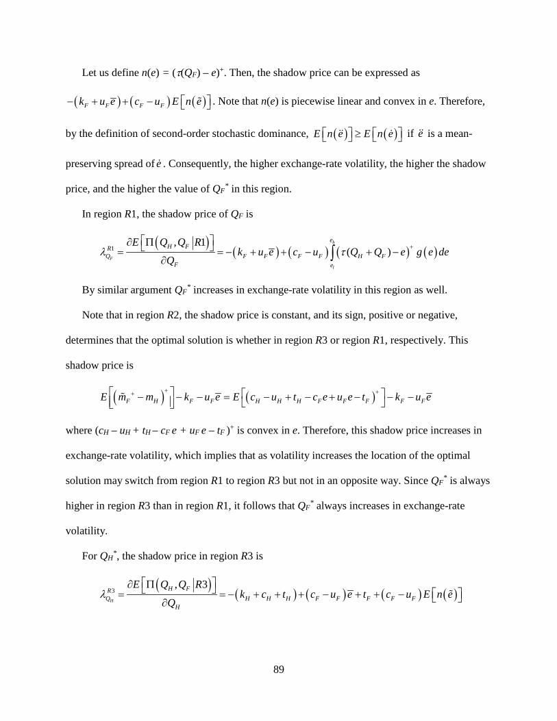
89

Let us define n(e) = (τ(QF) – e)+. Then, the shadow price can be expressed as

( ) ( ) ( )F F F Fk u e c u E n e − + + − . Note that n(e) is piecewise linear and convex in e. Therefore,

by the definition of second-order stochastic dominance, ( ) ( )E n e E n e ≥ if e is a mean-

preserving spread of e . Consequently, the higher exchange-rate volatility, the higher the shadow

price, and the higher the value of QF* in this region.

In region R1, the shadow price of QF is

( )

( ) ( ) ( ) ( )1 ( ), 1

F

l

hH F

e

H FR

Q F F F FF e

E Q Q Rk u e c u e g eQ de

QQλ τ +

∂ Π = = − + + − −+∂ ∫

By similar argument QF* increases in exchange-rate volatility in this region as well.

Note that in region R2, the shadow price is constant, and its sign, positive or negative,

determines that the optimal solution is whether in region R3 or region R1, respectively. This

shadow price is

( ) ( )F H H H HF F F F F F FE c uE m m k u e c e u et t k u e+ ++ − − − − + −= − + − −

where (cH – uH + tH – cF e + uF e – tF )+ is convex in e. Therefore, this shadow price increases in

exchange-rate volatility, which implies that as volatility increases the location of the optimal

solution may switch from region R1 to region R3 but not in an opposite way. Since QF* is always

higher in region R3 than in region R1, it follows that QF* always increases in exchange-rate

volatility.

For QH*, the shadow price in region R3 is

( )

( ) ( ) ( ) ( )3, 3

H

H FRQ H H H F F F F F

H

E Q Q Rk c t c u e t E n ec u

Qλ

∂ Π = = − + + + − + + − ∂

90

where n(e)=[(τ1 – e)+ –(e –τ (QH))+] is piecewise linear but neither convex nor concave in e,

which leads to an inconclusive result regarding the behavior of the domestic capacity in

exchange-rate volatility.

(b) From (2.5) using the Envelope Theorem, we have

( ) ( )

( )* *

* **2

2,

, | ,,

,

, ,,

, ||

, ,H H F F

H F H FH F

H F H Fq q q q

E q q Q QQ Q

E q q Q

x eee

xe

Qe

e

ππ

π= =

∂∂=

∂ ∂ ∂

= ∂

(A.11)

where

( ) ( ) ( )

{ } ( )

2 , | , ( )

mi

, ,

n ,h

l

H F H F H H H H F F F F

x

H Fx

E q q Q Q c u t q c u e t q

p x q q f x

x

d

e

x

π = − + − − +

+ +∫

We note that ( )2 , | ,, ,

( )H F H FF F F

x ee

E q q Q Qc u q

π − −∂

=∂

. Thus, from (A.11),

( )**,,

( )H FF F F

ee

Q Qc u q

π∂= − −

∂which implies ( )2

2

* *, ( )( ),H F F

F F

Q Q q ec ue

e eπ∂

=∂

∂− −

∂which is

positive because qF* decreases in e.

Consequently, ( )* , ,H FQ eQπ is convex in e, which by the definition of second-order

stochastic dominance implies ( ) ( )* *, ,, ,H F H FE Q Q eQ Qe Eπ π > if e is a mean-preserving

spread of e . As a result, the first-stage expected profit increases in exchange-rate volatility.

Proof of Proposition 2.10. From the first equation of the system of equations in (2.13) for

uniformly distributed exchange rate ( [ ]~ ,e U e d e d− + ), we have

( ) ( ) ( ) ( )( )1( )

1 1 2

( 02

)H

e d e d

F F F F F H HQ

H H H Hc u e de c e u eQ c u tt de k ud dτ τ

τ+ +

− −− − +− + − + + =∫ ∫

91

which simplifies to

( ) ( )( )( ) ( )

( )

22

) 04 4

( F F FF FH H

F F

H H HH

c u e d tc ue d k u

dc u t

Qd c u

τ − + + − − +

−− + − + + =

−

or

( )( )( ) ( ) ( )( )

( )

22

2) 4

( F F H H HF F F

FH

H H

F

c u e d t d c u kc ue d

c u

u tQτ

− + − + + − − − + + − =−

.

The feasible solution to this quadratic equation is

( ) ( )( ) ( ) ( )( )* 21 4 H HH F F F F F H HHF F

e d c u e d t c u t d c u k uc u

τ − + = + − − + + − − − + −

The square root term is guaranteed to be positive by OC4 which is required to hold under

policy DE. It follows that

( )( ) ( ) ( )

( )( ) ( ) ( )( )

*

2

21

4

F F F H HH H H

H H

H

F F F F FH H H

c u e d t k uc ud c u e d t d c u

t

c u t k u

τ − +

−

− + + − − +∂ = −∂ − + + − − − + +

.

The root of the above partial derivative occurs when

( )( ) ( ) ( )( )

( )( ) ( ) ( )( )

2

2

4

02

F F F F F H H

F F

H

F H H

H H

H H H

c u e d t d c u k u

c u

c u t

c ue d t k ut

− +

− − +

− + + − − − +

− + + − − + =

which reduces to (cF – uF) ē + tF – (kH + cH + tH) = 0. As a result, when kH + cH + tH < (cF – uF) ē

+ tF, we have *

0H

dτ∂

>∂

which by definition (τH *= τ (QH

*) = (p [(1 – F(QH*)] – tF)/ (cF – uF))

implies *

0HQd

∂<

∂.

Proof of Proposition 2.11. In case 1, by Proposition 2.6, the potentially optimal policies are FL,

FH, and DE. From Proposition 2.9, we know that the left-hand side (LHS) of OC2 and QF*

increase in exchange-rate volatility. As a result, the optimal policy can switch from FL in region

92

R1 to FH in region R3, and not in the opposite way. Depending on whether OC4 holds in region

R3, the optimal policy may change to DE.

In case 2, all policies can potentially be optimal. At sufficiently low degrees of exchange-rate

volatility, the firm adopts policy H due to the lower cost of onshore sourcing. Note that under

policy H, when OC1 does not hold, OC2 does not hold either. Moreover, if OC1 does not hold,

OC3 holds because

( )

0

F F H H F F

F

H F H

F H F

F k u e kE m m E mu k u e

k uM e

M

E m

+ +

++

− − − = − −

< − − <

− − −

−

. (A.12)

Higher levels of exchange-rate volatility cause the LHS of OC1 to increase (by similar

argument as presented in proof of proposition 2.9) until OC1 holds. Observe that due to

inequality (A.12), at this switching point, OC3 still holds. This is where DR becomes the optimal

policy. As exchange-rate volatility increases, the LHS of OC2 increases and the LHS of OC3

decreases. The latter is because mF+ is convex in e, thus ( )HF HF F Hk u e km uE m + − − − −−

increases in exchange-rate volatility by a similar argument as mentioned in proof of Proposition

2.9. Depending on whether OC3 does not hold or OC2 holds first, the optimal policy path is

different. If OC3 does not hold first, FL becomes the optimal policy first and similar to case 1,

the next optimal policies are FH (when OC2 holds) and DE if OC4 holds as well. Otherwise, if

OC2 holds before OC3 is reversed, the optimal solution moves to R3. But this also causes OC4

to hold because the LHS of OC4 is the summation of the LHS of OC2 and that of OC3.

Therefore, if both OC2 and OC3 hold, OC4 holds as well. That implies that the optimal solution

may directly switch from DR to DE.

Proof of Proposition 2.12. (a) For eα ≥ τ2, we have qF*(eα) = 0. By supposition, we have

( ) ( ),*0, Fe x QP β α < − >Π .

93

Furthermore,

( )0 |, AFQ eαΠ = β− , ( )0 |, A

FQ eΠ < β− for all e > eα, ( )0 |, AFQ eΠ > β− for all e < eα,

and thus, ( ) ( ), 0, AFe x QP β α < − =Π .

Define

( )AF HQ Q ≡ ( ) ( ) [ ] ( )H H H H F F H H F Fp k c t Q k u e M Q k u eα αβ β − − − + = + + + (A.13)

and note that ( ) ( )( ), , AF He x HQ Q QP β α < − =Π for all 0 ≤ QH ≤ xL.

(a) If AFQ = ( )0A

FQ > qH0, we can substitute the capacity investment in (A.13) into the first-

stage objective function associated with R3 and take its first-order derivative with respect to QH.

The total derivative of that function with respect to QH can be expressed as:

( )( ) ( )( )

( ) ( )( )

, 3 , 3 ,.

3| |A A

F H F H

A AF H F FF H

Q Q Q QH

H H

H H

H

F

Q Q E Q E QdQ QQ d

dE Q R Q R Q RdQ Q Q

∂ ∂= +

∂

Π∂

Π Π

From Proposition 2A.4,

( )( ) ( ) ( ) ( )

( ), 3( )

l

FQH F

F F F F FF e

E Q Q Rk u e c u Q e g e de

Q

τ

τ ∂ Π = − + + − −

∂ ∫ , and,

( )( ) ( ) ( ) ( ) ( )

( )

, 3( )

h

H

eH F

H H F F H H FH Q

E Q Q Rk u c u e Q g e de E m m

Q τ

τ + ∂ Π = − + − − − + − ∂ ∫ .

Thus,

94

( )( )

( ) ( ) ( )( )( )( )( )

( ) ( ) ( ) ( ) ( )2

0

2

, 3|

(

)

A

l

h

F

H

H

HQ

AF H

Q QAH

F F F F

H

e

H H

F HF F e

F F H F

Q Q

d

dE Q R

Q

k u

M k u e c u Q Q e g e dek u

c u e g e de E m m

e

τ

τ

α

τ

τ +

=

Π =

− + − − −

− + + − − +

+ − ∫

∫

Because the last two terms simplify to ( )H FE m m + + − , we can rewrite the derivative as

( )( )( )

( ) ( )( )( )( )( )

( )

0(

3|

)

,H

AF H

l

HQ

H

H F H H

F FAF H Q QH

AF F F F F H

e

k u ed Q Q M

d k u e c u Q Q

E Q

e g e d

R

Q

E m m u

e

k

τ

α τ=

+ +

Π =

−

− +

− −

+ + − −

+

∫

Note that the first term is positive since QFA < QF

0, and the last three terms form the LHS of

OC4 is negative because of the definition of policy FH. Because ( ) ( ) ( )l le e

e g e de G e deτ τ

τ − =∫ ∫ , the

above condition is equivalent to RA1. Therefore, when QFA > qH

0, if RA1 holds, the firm

satisfies the VaR constraint and increases expected profit by increasing QH from 0 to any QH ∈

(0, xL] while simultaneously increasing QF from ( )0AFQ to ( )A

F HQ Q , and thus engages in dual

sourcing under risk aversion.

(b) If AFQ = ( )0A

FQ ≤ qH0, regardless of whether FH or FL is the optimal policy in the risk-

neutral setting, we can substitute the capacity investment in (A.13) into the first-stage objective

function associated with R1 and take its first-order derivative with respect to QH:

( )( ) ( )( )

( ) ( )( )

, 1 , 1 ,.

1| |A A

F H F H

A AF H F FF H

Q Q Q QH H

H

H

HH F

d Q Q E Q E QdQ Qd Q d

E Q R Q R Q RQ Q Q

∂ ∂= +

∂

∂

Π Π Π

95

From Proposition 2A.2,

( )( ) ( ) ( ) ( )

( ), 1( )

H F

l

Q QH F

F F F F H FF e

E Q Q Rk u e c u t Q Q e g e de

Q

τ + ∂ Π = − + + − + −∂ ∫ , and,

( )( ) ( ) ( ) ( ) ( )

( ) ( ) ( )

( )

( )

, 1( )

( )

h

H

H F

l

eH F

H H H F F F F HH Q

Q Q

F F H Fe

F

E Q Q Rk c t c u c u e Q g e de

Q

c u Q Q e g e

e

de

tτ

τ

τ

τ+

∂ Π = − + + + − − − −∂

+ − + −

+ ∫

∫

Thus,

( )( )

( ) ( ) ( )( )( ) ( )( )( )

( )( )( )

( )( ) ( )

0

,

(

|

)

1

AF H

l

A

H

l

F H

AF H

Q QAH

F F F F F HF F e

Q Q

HQ

H

AF HH F F F

e

Q Q

M k u e c u Q Q e g e e de

dE Q R

dQ

M E m

k u e

c Q eQu e g deτ

τ

τ

τ

=

+

Π =

− + − −

− + + − − +

+

∫

∫

Therefore, when QFA ≤ qH

0 and dual sourcing is the optimal sourcing policy under risk

aversion if

( ) ( ) ( )( )( ) ( )( )( )

( )( )( )

( )( ) ( )

, ,

, ,

, , ( )

, , 0

AF H

l

AF H

l

Q Q eAH

F F F F F HF F e

Q Q eAF

eHH F F F

M k u e c u Q Q e e

M E m c u e g e d

g e e dek u e

Q Q e e

α

α

τ β

α

β

α

τ

τ β

βτ+

− + + − − +

− + − − >

+ ∫

∫

,

due to submodularity of the expected profit function, LHS of RA2 is larger than that of RA1.

Thus, under risk aversion, it is more likely for dual sourcing to be adopted when QFA ≤ qH

0 than

when QFA > qH

0.

96

Proof of Proposition 2.13. (a) Recall that eα denotes the exchange rate realization at fractile 1 –

α (i.e., [1 – G(eα)] = α). The realized profit is greater than or equal to –β when the exchange-rate

random variable takes values in the range el ≤ e ≤ eα, and the probability of loss greater than or

equal to β is less than or equal to α. In (2.20), we can equate the profit at e = eα inside the

probability expression to –β in order to determine the number of hedging contracts necessary to

warrant profitability that satisfies the VaR requirement:

( ) ( ) ( ) ( ) ( )

( )( ) ( )( ) ( ) ( ) ( ){ }

* *

* * * *min ,

H H F F H H H F F F

H H H F F F s H F

sk Q k Q c t q e c e t q e

u Q q e u e Q q e e e H p x q

h

e

H

e

e

q

α α α

α α α α α α

β+ +

− − − + − + = − − − − + − + +

−− .

Solving for H at the lowest demand realization x = xl provides the minimum (optimal)

number of hedging contracts satisfying VaR at e = eα:

( )

( ) ( ) ( ) ( )

( )( ) ( )( ) ( ) ( ){ }( )( )

* *

* * * **

min ,

H H F F H H H F F F

H H H F F F l F

ss

H

s

k Q k Q c t q e c e t q e

u Q q e u e Q q e p x q eH e

q e

e he e

α α α

α α α α α

α

β+ +

+ + + + +

+ − + − − + − − −

= .

(b) Taking the expectation of the term (e – es)H in (2.19) over all exchange-rate realizations

provides the expected return of ( ) ( )h

l

e

se

H e e g e de

− ∫ in stage 2, which is equal to the first-stage

payment of ( ) ( ) ( ) ( ) ( ) ( ) ( )h s h

s l l

e e e

s s s se e e

h e H H e e g e de e e g e de H e e g e de

= − − − = − ∫ ∫ ∫ for H

units of hedging contracts in (2.18). Thus, the expected profit for any given (QH, QF) decision

made in stage 1 in the risk-neutral setting can be replicated through purchasing H*(es) units of

contracts in (2.21) under risk aversion to satisfy VaR.

97

98

Appendix to Chapter 3

Proof of Proposition 3.1. The first- and second-order derivatives of the second-stage profit

function (3.4) with respect to q are respectively:

( ) ( ) ( )

22

22

( ) ln( )

( ) 0

sd q M q Mv s

dq k q M q

d q M M Mdq q M q q M qM q

π ββϕ

π β β β

−= − + − −

= − − = − <

− −−

Thus, as shown in Proposition 1 in Noparumpa et al. (2015) for a similar problem, π(q) is

concave in q. The unconstrained optimal processing quantity q0(φ) can then be obtained from the

first order condition (FOC) (We use superscript “0” for the optimal decisions associated with the

problem where there is no supply constraint). That is, q0 (φ) solves

ln 0( )s

M q Mv sk q M q

ββϕ

−− + − = −

which implies ( )

sv sMM qM q e

k qβ

ϕ

−−

−−= . We rearrange to get

( )/ 1 / ( )s

qv sM qq e e k

M qβ ϕ− −− =

− which conforms to the Lambert W function structure. Thus,

( )( )/ 1 / ( )sv sq W e kM q

β ϕ− −=−

which implies

( )( )( )/ 1

0( )/ 1

/ ( )( ) ( )

1 / ( )

s

s

v s

v s

W e kq M M

W e k

β

β

ϕϕ α ϕ

ϕ

− −

− −= =

+ (A.14)

Substituting (A.14) into (3.2), we get

( ) ( )( )/ 10( )/ 1

1( ) ln ln ( ) / ( )( ) / ( )

s

s

v ss sv s

p v v k W e kk W e k

ββ

ϕ β β ϕ ϕϕ ϕ

− −− −

= + = −

.

Note that by the definition of the Lambert W function ( )( ) W zW z e z= , which implies

( )( ) ( ) ( )W zk W z e k zϕ ϕ= , and thus [ ] [ ]ln ( ) ( ) ( ) ln ( )k W z W z k zϕ ϕ+ = . Let ( )/ 1 / ( )sv sz e kβ ϕ− −= . It

99

follows that ( ) ( )( )/ 1 ( )/ 1 ( )/ 1ln ( ) / ( ) / ( ) ln ( ) / 1s s sv s v s v ssk W e k W e k e v sβ β βϕ ϕ ϕ β− − − − − − + = = − − .

Therefore, we can re-write p0(φ) as

( )( )

( )/ 10

( )/ 1

( ) ( ) / 1 / ( )

1 / ( )

s

s

v ss s

v s

p v v s W e k

s W e k

β

β

ϕ β β ϕ

β ϕ

− −

− −

= − − − − = + +

Therefore, if Qy ≥ q0(φ), q*(φ) = q0(φ) , p*(φ) = p0(φ) , and the optimal second-stage profit is

( ) ( ) ( )( )/ 1* , , / ( )sv sQ y W e k s r QM yβπ ϕ β ϕ− −= + −

which results from substituting (A.14) into (3.4).

Otherwise, if Qy < q0(φ), due to concavity of π(q), q*(φ) = Qy, and equations (3.2) and (3.4)

yield p*(φ) and π*(Q,y,φ), respectively.

Proof of Proposition 3.2. If Qy < Mα(φ), taking the first-order derivative of p*(φ, y) expressed

in Proposition 3.1 with respect to φ, we get

( )/* '

( )/( , ) ( ) 11 if ( )

( ) 1 ( )

c

c

v

vp y k e Qy M

k e k

ϕ β

ϕ β

ϕ ϕβ α ϕϕ ϕ ϕ

−

−

∂ −= = = − <

∂ + (A.15)

where the last two equalities use the definition of k(φ) by (3.3).

If Qy ≥ Mα(φ), we have

*( ) ( ) ( ).p dW z dzdz d

ϕ ϕβϕ ϕ

∂=

∂ (A.16)

where ( )/ 1( ) / ( )sv sz e kβϕ ϕ− −= . In order to find dW(z)/dz, we take the derivative of both sides of

( )( ) W zW z e z= with respect to z (Noparumpa et al. 2015) to get ' ( ) ( )( ) ( ) 1W z W zW z e W z e + =

which yields

[ ]( ) ( ) ( )

1 ( ) ( )dW z W z

dz z W z zα ϕ

ϕ= =

+ (A.17)

100

We then find the derivative of z(φ) with respect to φ as

' '( )/ 1

2( ) ( ) ( ) ( ) ( ) 11

( ) ( ) ( )sv sdz k k z ze

d k k kβϕ ϕ ϕ ϕ ϕ

ϕ ϕ ϕ β ϕ− − − −

= = = −

(A.18)

Therefore, substituting (A.17) and (A.18) into (A.16), we get

*( , ) 1( ) 1 if ( )( )

p y Qy Mk

ϕ α ϕ α ϕϕ ϕ

∂= − ≥ ∂

(A.19)

Note that by definition, α(φ) < 1 (Proposition 3.1), and k(φ) > 1 (equation (3.3)). Therefore,

(A.15) and (A.19) imply that ∂p*(φ,y)/∂φ < 1.

Proof of Proposition 3.3. From Proposition 3.1, we can re-write α(φ) expression as

( ) ( )( ) / 1W z W zα ϕ = + where ( )/ 1 / ( )sv sz e kβ ϕ− −= . By chain rule, we have

( ) ( ) ( ) ( ). .d d W dW z dzd dW dz dα ϕ α ϕ

ϕ ϕ= (A.20)

The first derivative on the right-hand side (RHS) is

[ ]2( ) 1

1 ( )d W

dW W zα

=+

(A.21)

Using the derivations in the proof of Proposition 3.2, we substitute (A.21), (A.17), and

(A.18) into (A.20) to get

[ ]3( ) ( ) 11

( )1 ( )d W z

d kW zα ϕ

ϕ ϕβ

= − +

which is positive. The results follow.

Proof of Proposition 3.4. (a) The first-order derivative of the expected profit function (3.5) with

respect to Q is

101

( ) ( )( )

( )

ln ( ) ( )( )

( ) ( )

sU Q

O Q

M Qy Ml ry y v g y h dydQ k Qy M Qy

syg y h dy

Q

d

β β ϕ ϕϕ

ϕ ϕ

−− + + + − −

Π

+

∂=

∂ ∫∫

∫∫

and the second-order derivative with respect to Q is:

( )2

2

)

2

(

( ) ( ) 0U Q

y M g y h dydQ Q M Qy

Q β ϕ ϕ −

< −

∂

Π=

∂ ∫∫ .

Consequently, the expected profit function is concave in Q and (3.6) is the FOC which yields

the unique optimal leasing quantity.

(b) By substituting Q* into (3.5) and rearranging, the optimal expected profit can be

expressed as:

( ) ( )

*

*

* *

* *

*

* ** ( )

( )

( )/ 1*

*( ) ( )

ln ( ) ( )( )

( ) ( )

( ) ( ) ( ) ( )( )

s

sU Q

O Q

v s

U Q O Q

Q l ry Q

M Q y My v g y h dydk Q y M Q yQ

syg y h dyd

Q y eM g y h dyd W g y h dydM Q y k

β

β β ϕ ϕϕ

ϕ ϕ

β ϕ ϕ ϕ ϕϕ

− −

∏ = − +

−+ − − +

+

+ + −

∫∫

∫∫

∫∫ ∫∫

(A.22)

Substituting the FOC (3.6) into (A.22), the first two terms cancel out, which results in (3.7).

Proof of Remark 3.1. ( ) /DQ M yα ϕ= is larger than ( ) /Tl hQ M yα ϕ= , because hy y< , and

according to proposition 3.3, 1ϕ ϕ> implies 1( ) ( )α ϕ α ϕ> .

Proof of Proposition 3.5. (a) Note that according to Proposition 3.3, the processor targets the

smallest portion of the high-end segment when the commodity price is realized at its lowest level

(φl). Therefore, the processor underinvests in DT if and only if Q*yh < Mα(φl), i.e., the first-order

102

derivative of the (first-stage) expected profit function with respect to Q evaluated at Mα(φl)/ yh

must be negative (Note that in this case Qy < Mα(φ) for all realizations of y and φ):

( ) ( )( )

( )ln ( ) ( ) 0( ) ( ) ( )

|l

h

h l hs

l h lAyM

y y yl ry y v g y h dydQ k y yQ

yϕαα ϕβ β ϕ ϕ

ϕ α ϕ α ϕ −

− + + + − < −

∂Π=

∂ ∫∫

which results in condition (3.8).

(b) When the processor adopts the underinvestment policy, the crop supply always falls short

of the optimal demand and the processor sets a market-clearing price in the second stage, which

results in the optimal second-stage profit as expressed below:

( )* , , ln( )

U sM QyQ y v rk Q

yy

Qπ ϕ βϕ

−− +

=

Therefore, the first-stage expected profit function can be expressed as:

( ) ( )

ln ( ) ( )( )U s

A

M Qyl ry Q Qy v g y h dydk Qy

Q β ϕ ϕϕ

−∏ = − + + +

∫∫ (A.23)

From Proposition 3.4, we can infer that ΠU(Q) is concave in Q, and thus the below FOC

yields the optimal leasing quantity (QU*).

( )

ln ( ) ( ) 0( )

Us

A

M Qy My y v g y h dydQ k Qy

QQ

lM

ry

β β ϕ ϕϕ

−+ + − = −

∂Π= − −

∂ ∫∫ (A.24)

(c) Note that by substituting QU* into (A.23) and rearranging, the optimal expected profit can

be written as:

( ) ( )*

* * ** *

*

*

ln ( ) ( )( )

( ) ( )

UU U U

U U

U

U

U sA

A

M y Ml ry y v g y h dydk y M y

yM g y h

QQ Q QQ Q

d dQ yyM Q

β β ϕ ϕϕ

β ϕ ϕ

−∏ = − + + −

+ −

−

+

∫∫

∫∫

Substituting (A.24) into (A.23), the first two terms cancel out, and we get (3.10):

103

( )* *

*

*

* ( ) ( ) ( )

h

l

y

UA y

U UU

U U

y yM g y h dyd M g y dyy

Q QQM yM Q Q

β ϕ ϕ β∏ = =− −∫∫ ∫ .

(d) QU* < QT

directly follows from part (a).

Proof of Proposition 3.6. (a) Condition (3.8) can be expressed as

( )( , ) 0Yl ry E E n YΨ − − + Φ < , where

[ ] [ ]

( )( , ) ln( ) ( ) ( )

ln ( ) ln ( ) ( )( )

h h hs

h h h

hs h h h

h h

y y yn y y vk y y y

yy v y y k yy y

α ϕϕ β βϕ α ϕ α ϕ

β α ϕ β ϕ α ϕ βα ϕ

−= + − −

= + − − − −

(A.25)

Note that n(y, φ) is concave in y. This is because

( )2

2

( ) ( ) ( )( , ) 1ln( ) ( ) ( ) ( ) ( )

( )ln( ) ( ) ( ) ( )

h h h h h hs

h h h h h h h

h h h hs

h h h h h

y y y yn y v yy k y y y y y y y y

y y y yvk y y y y y

α ϕ α ϕ α ϕϕ β β βϕ α ϕ α ϕ α ϕ α ϕ

α ϕβ β βϕ α ϕ α ϕ α ϕ

− −∂ = + − + − − ∂ − − −

−= + − − − −

and thus,

( ) ( )

22

2 32

( ) ( ) 2 ( )( , ) 1 0( ) ( ) ( )

h h h h h

h h h h h h

y yn yy y y y y y y y

α ϕ α ϕ α ϕϕ βα ϕ α ϕ α ϕ

∂ = − + + + < ∂ − − −

which is negative because by definition, yh > y, and 0 < α(φ) < 1 (Proposition 3.1), and thus yh >

α(φh) y which implies the first and the last term within the parenthesis are positive. As a result,

by the definition of second-order stochastic dominance, EY[n(Y2, Φ)] < EY[n(Y1, Φ)] if Y2 is a

mean-preserving spread of Y1. This implies that, as the degree of yield uncertainty increases, the

left-hand side (LHS) of (3.8) decreases, which means (3.8) eventually holds as the variation

increases, if it holds when the random yield features the highest possible variation, i.e., two-point

distribution.

104

We take an analogous approach to prove the LHS of (3.8) decreases in commercial price

uncertainty. We rewrite condition (3.8) as ( )( , ) 0Yl ry E E n YΨ − − + Φ < , where n(y, φ) is

defined by (A.25), and show that n(y, φ) is concave in φ. We have

'( , ) ( ) 11( ) ( )

n y ky yk k

ϕ ϕβϕ ϕ ϕ

∂= − = − ∂

and thus,

2 '

2 2( , ) ( ) 11 0

( ) ( )n y k yy

k kϕ ϕ

ϕ ϕ β ϕ ∂ −

= = − < ∂

which is negative since by definition, k(φ) > 1 (equation (3.3)). Therefore, the results follow.

(b) We demonstrate that ( ) ( )* *U UQ Q∏ < ∏ . Rewriting (3.7) and (3.10), we express the

difference as:

( ) ( )*

*

*

( )/ ( )/ 1*

*( )/

( )/ *

*

( )/

* *

*

*

*

1

*

( ) ( ) ( )( )

( ) ( )

( )

( )

h h s

l l

h h

l l

l

s

U

U

yM Q v s

Uy

U

M Q

y

y

M QU

y U

v s

Q y eM g y dy W g y dy h dM Q y k

yM g y h dydy

yQ y g y d

Q Q

Q

yM Q y y

MeW

k

M Q

QM Q

ϕ α ϕ β

ϕ α ϕ

ϕ

ϕ

α ϕ

β

β ϕ ϕϕ

β ϕ ϕ

β

ϕ

− −

− −

∏ − ∏ = + −

−

− −

=

+ −

−

−

∫ ∫ ∫

∫ ∫

∫

*

*

*( )/

( ) ,

( )

h

hl

y

M Q

U

U

QM

h dy g y dy

yQ

ϕ

ϕ

α ϕ

ϕ ϕ

−

∫∫

and make two observations. First, the first term within the bracket is positive because QU* < Q*.

Second, the second term within the bracket is also positive, because QU* y < Mα(φ) for any

realizations of y and φ by the definition of underinvestment, and thus,

( )* /

*

1( ) ( )( ) 1 ( ) ( )

sv sU

U

y M eWy M M k

QM Q

βα ϕ α ϕα ϕ α ϕ ϕ

− − < = = − − −

105

As a result, ( ) ( )* * 0U UQ Q∏ − ∏ > .

Proof of Proposition 3.7. When the commercial price is deterministic and the processor

encounters only yield uncertainty, we can replace φ with ϕ in all expressions of Proposition 3.1

including the optimal second-stage profit function expressions as follows:

( )( ) ( )

*

( )/ 1

if (

if

ln )( ), ,

/ ( ) ( )s

s

v s

M Qyv rk QyQ

Qy Qyy

W e k s r Qy

M

M Qy Mβ

β ϕϕπ ϕ

β ϕ ϕ

α

α− −

−− +

+ −

< =

≥

Consequently, the first-stage expected profit function can be written as

( ) ( ))/

( )

(

/

/(

1

)

ln ( )( )

( )( )

l

h s

Q

sy

y v s

Q

M

M

M Qyl ry Q Qy v g y dyk Qy

eW sQy g y dyk

Q

M

ϕ

ϕ

β

ϕ

α

α

βϕ

βϕ

− −

−∏ = − + + +

+ +

∫

∫

and thus,

( ) (

(

)/

)/

ln ( ) ( )( )

l

hM

y M

yQ

sQ

M Qy My v g y dy syg y dyQ k Qy M Qy

Qϕα

α

ϕ

ϕ

β βϕ

−+ − + −

∂Π

=

∂ ∫∫

Therefore, the processor underinvests if and only if * ( )hQ y Mα ϕ< , or

( ))(

(| 0(

)ln ( )( ) ) )(

h

h

l

h hs

hy

y

My

y y yy v g y dyQ k y

Ql r

y yyϕ

ϕαϕβ β

ϕ ϕ ϕαα α

−+ −

∂Π= −

− − +∂

<∫ . (A.26)

When the yield is deterministic, and the processor encounters only commercial price

uncertainty, the optimal second-stage profit function becomes (note that α(φ) is an increasing

function of φ) :

( )( ) ( )( )/ 1

*

ˆ/ ( ) ( ) (or ))

, ,ˆln

if (

i ( ) (or ))(

f ()

sv s

s

W e k s r Qy Q y

Q y M Qyy

M Q M

Q v r Qk

MQ

Qyy

ββ ϕ ϕ ϕ ϕ

π ϕβ ϕ ϕ ϕ

ϕ

α

α

− − + − ≤

−− + >

≥=

<

106

The first-stage expected profit function can then be written as:

( ) ( )ˆ ( ) ( )/ 1

ˆ ( )

( )( )

ln ( )( )

s

l

h

Q v s

y

sQ

el ry Q W sQyQ M h dk

M QyQy v h dk Qy

ϕ β

ϕ

ϕ

ϕ

β ϕ ϕϕ

β ϕ ϕϕ

− − ∏ = − + + +

−+ +

∫

∫

and,

( ) ˆ ( )

ˆ ( )

( ) ln ( )( )

h

l

Qy

sQ

M Qy Msyh d y v h dQ k Qy M

QQy

ϕϕ

ϕ ϕ

ϕ ϕ β β ϕ ϕϕ

−+ + − −

∂Π

=

∂ ∫ ∫

Therefore, the processor underinvests if and only if * ( )lQ y Mα ϕ< , or

( )

( )( )

)

( )/ 1

( )/ 1

(1 ) 1ln ( )( ) ) 1 )

ln ( ) / ( )( )

1

(|( (

/0

( )

h

l

l

sh

sl

y ls

l ly

v ss

v s

M

Ql ry y

l r

v h dQ k

v k W e kh d

e ky

Wy

α

ϕ

ϕϕ

βϕ

βϕ

αα α

ϕβ β ϕ ϕϕ ϕ ϕ

β ϕ ϕϕ ϕ

β ϕ

− −

− −

−+ − −

−

∂Π= − − +

∂

= − − + − +

<

∫

∫

Note that by the definition of the Lambert W function ( )( ) lW zl lW z e z= , which implies

( )( ) ( ) ( )lW zl l l lk W z e k zϕ ϕ= , and thus [ ] [ ]ln ( ) ( ) ( ) ln ( )l l l l lk W z W z k zϕ ϕ+ = . Let

( )/ 1 / ( )sv sl lz e kβ ϕ− −= . It follows that

( ) ( )( )/ 1 ( )/ 1 ( )/ 1( )ln ( ) / ( ) / ( ) ln ( ) / 1( )

s s sv s v s v sll l s

k k W e k W e k e v sk

β β βϕ ϕ ϕ ϕ βϕ

− − − − − − + = = − − , or

( ) ( ) [ ]( )/ 1 ( )/ 1ln ( ) / ( ) ( ) / 1 / ( ) ln ( ) / ( )s sv s v sl s l lk W e k v s W e k k kβ βϕ ϕ β ϕ ϕ ϕ− − − − = − − + − . Thus, we

can simplify the above condition to

( ) [ ]( )| ( ln ( ) / ( )) 0( )h

l

l

ly

M k k h dQ

s r yQ

l yϕ

ϕα ϕ

ϕ

β ϕ ϕ ϕ ϕ∂Π

= − + − + <∂ ∫ . (A.27)

107

As a result, conditions (A.26) and (A.27) show that uncertainty in either yield or commercial

price by itself can lead to the underinvestment policy.

Proof of Proposition 3.8. (a) The FOC for the underinvestment policy (3.9) can be re-written as:

[ ], ( , , ) 0Y Ul ry E n Q YΨ− − + Φ = (A.28)

where ( ), , ln( )U s

M Qy Mn Q y y vk Qy M Qy

ϕ β βϕ

−= + − −

. Due to a similar argument presented in

the proof of proposition 3.6, if we show that nU (Q,y,φ) is concave in y and φ, the LHS of (A.28)

decreases in yield and commercial price uncertainty, respectively, and thus, the optimal leasing

quantity must decrease in the level of uncertainty in order to satisfy the FOC (due to concavity of

the expected profit function).

We observe that nU (Q,y,φ) is indeed concave in both y and φ, because

( )( ) ( )

( )( )

2

2

2

, ,ln

( )

ln( )

2ln

( )

Us

s

s

Q y M Qy M M MQv yy k Qy M Qy y M Qy M Qy

M Qy M Mvk Qy M Qy M Qy

M M QyM Qy

n

vk Qy M Qy

ϕβ β β

ϕ

β β βϕ

β βϕ

− + − + − − − − −

−= + − − − −

− −= + −

∂

−

=∂

( )( )

( )( )

( )( )32

2 2, 30

,U Q y MQ M QyMy y M Qy M Qy

n M M Qyy M Qy

ϕ ββ

−

∂ − += − = <

∂ − −+

−

and,

'( , , ) ( ) 11( ) ( )

Un Q y ky yk k

ϕ ϕβϕ ϕ ϕ

∂= − = − ∂

2 '

2 2

( , , ) ( ) 0( )

Un Q y kyk

ϕ ϕϕ ϕ

∂= <

∂.

108

(b) When the underinvestment policy is optimal, the first-stage expected profit function in

(A.23) can be expressed as:

( ) [ ], ( , , )Y Ul ry Q E m Q YΨ− + + Φ , where ( , , ) ln( )U s

M Qym Q Y Qy vk Qy

βϕ

−Φ = +

.

We show mU (Q,y,φ) is concave in both y and φ, and thus due to a similar argument

developed in the proof of proposition 3.6, the first-stage expected profit decreases in the yield

and commercial price variation. Note that

( )

( )( ) ( )2

2

2

2

, ,ln ,

( )

, ,

0

Us

U

Q y M Qy Mvy k Qy M Qy

Q y M MQy M Qy

mQ

my M Qy

My

Q

MQ

Qy

ϕβ β

ϕ

ϕβ

β

−+ − − = − + − −

= − < −

∂

∂=

∂

∂

and,

( )

( )2

'

'

2 2

, , ( ) 11 ,( ) ( )

0, , ( )

( )

U

U

mQy

mQy

Q y k Qyk k

Q y kk

ϕ ϕβϕ ϕ ϕ

ϕ ϕϕ ϕ

− = −

∂=

∂

∂

= <∂

Hence, the results follow.

Proof of Proposition 3.9. (a) The first-order derivative of the first-stage expected profit function

(3.11) with respect to Q is

( )( )

ˆ ( )

ˆ ( )

ln ( ) ( )( )

h

l

yy Qpc

syy Q

M Qy My v g y dy syg y dyQ k y Qy M y

QQ

l ry β βϕ

−+ − + −

∂Π= − − +

∂ ∫∫

and thus, the processor underinvests if and only if ( )* ( ) ( )pc h h lQ y M y Mα ϕ α ϕ< = , or

109

( ) ( ))(

((

| 0

(

)ln( ) )

( )

)h l

l

h

h ls

pc l

y

h

y

y h

l

M

y yvk y yQ

l y g y dyQ y

y y

ryϕα

ϕβϕ ϕ

βϕ

αα

α

∂Π= −

−+

− −

+∂

− <∫ (A.29)

Next, we compare (A.29) with its corresponding condition in the case of less-than-perfect

correlation where Φ(y) is the random commercial price with E[Φ(y)] = φ(y). Note that the LHS

of (A.29) can then be written as:

[ ]( )( )ln ( )

)( ) )

)ln ( , )( ) ) )

((

(( (

h

hh

l

l

l

h l hs

h ll

y

y

h l hs

l h l

y

y

y y yy v g y dyy yk E y y

y y yy v y

l ry

l r dyk y y y

y dϕ

ϕ

ϕβ βϕϕ

ϕβ β ω ϕ ϕϕ ϕ ϕ

ααα

αα α

− − +

> − −

− + − −Φ

−+ −

+−

∫

∫ ∫ (A.30)

where the inequality holds due to Jensen’s inequality and the fact that the term

)ln( ) ) ( )

((

h l hs

l h l

y y yy vk y y y

ϕβ βϕ ϕ ϕ

αα α

−+ − −

within the integrals is concave in φ. We note that

under less-than-perfect correlation (including the case of two independent random variables), it

is optimal for the processor to underinvest if the RHS of the above inequality becomes negative.

i.e.,

( ))(

)ln ( , ) 0(

|)

(() )(

h

l

lh

h

l

lc h ly

hs

l h lM

y y

Ql ry dy y yy v y dy

Q k y y y

ϕ

ϕϕ

αϕβ β ω ϕ ϕ

ϕ ϕ ϕαα α

−+ − < −

∂Π= − − +

∂ ∫ ∫ .

As a result, (A.30) implies that if underinvestment is optimal under perfect correlation, it

must be optimal under less-than-perfect correlation as well.

(b) When the underinvestment policy is optimal, denoting the first-stage expected profit

function under perfect correlation by ( )Upc Q∏ , and that under less-than-perfect correlation by

( )Ulc Q∏ , we have

110

( ) ( ) ( )

( ) [ ]( )

( ) ( )

ln ( )( )

ln ( )( )

ln ( , )( )

h

l

h

l

h h

l l

y

Upc sy

y

sy

y

s Ulcy

M Qyl ry Q Qy v g y dyk y Qy

M Qyl ry Q Qy v g y dyk E y Qy

M Qyl ry Q Qy v y dydk Qy

Q

Qϕ

ϕ

βϕ

β

β ω ϕ ϕϕ

−∏ = − + + +

− = − + + + Φ

−> − + + + = ∏

∫

∫

∫ ∫

where the inequality holds due to Jensen’s inequality and the fact that the term

ln( )s

M QyQy vk Qy

βϕ

−+

within the integrals is concave in φ.

111

REFERENCES

Allon, G., J. A. Van Mieghem. 2010. Global dual sourcing: tailored base-surge allocation to

near- and offshore production. Management Science 56(1) 110–124.

Anupindi, R., R. Akella. 1993. Diversification under supply uncertainty. Management Science

39(8) 994–963.

Basel Committee on Banking Supervision. 2013. International convergence of capital

measurement and capital standards: A revised framework. Bank for International

Settlements, Press & Communications, CH-4002 Basel, Switzerland.

Boyabatlı, O., P. R. Kleindorfer, S. R. Koontz. 2011. Integrating long-term and short-term

contracting in beef supply chains. Management Science 57(10) 1771–1787.

Boyabatlı, O. 2015. Supply Management in Multiproduct Firms with Fixed Proportions

Technology. Management Science 61(12) 3013–3031.

Burke, G., J. E. Carrilo, A. J. Vakharia. 2009. Sourcing decisions with stochastic supplier

reliability and stochastic demand. Production and Operations Management 18(4) 475-484.

Chen, L., R.O. Roundy, R.Q. Zhang, L.W. Robinson. 2015. New sufficient conditions on (s, S)

policies to be optimal in systems with multiple uncertainties. Operations Research 63(1)

186-197.

Chen, L., S. Li, L. Wang. 2014. Capacity planning with financial and operational hedging in

low-cost countries. Production and Operations Management 23(9) 1495-1510.

Cohen, M. A., T. H. Ho, Z. J. Ren, C. Terwiesch. 2003. Measuring imputed cost in the

semiconductor equipment supply chain. Management Science 49(12) 1653–1670.

Corless, R. M., G. H. Gonnet, D. E. G. Hare, D. J. Jeffrey, D. E. Knuth (1996) On the Lambert

W function. Advances in Computational Mathematics 5(1) 329–359.

112

Craymer, L. 2015. Chaina’s Changing Tastes Offer Upside for Coffee. Wall Street Journal.

Dada, M. N., C. Petruzzi, L. B. Schwarz. 2007. A newsvendor’s procurement problem when

suppliers are unreliable. Manufacturing and Service Operations Management 9(1) 9–32.

Ellram, L. M., W. L. Tate, K. J. Petersen. 2013. Offshoring and reshoring: An update on the

manufacturing location decision. Journal of Supply Chain Management 49(2) 14-22.

Erkoç, M., D. Wu. 2005. Managing high-tech capacity expansion via reservation contracts.

Production and Operations Management 14(2) 232-251.

Feng, Q. 2010. Integrating Dynamic Pricing and Replenishment Decisions Under Supply

Capacity Uncertainty. Management Science 56(12) 2154-2172.

Feng, Q., L.X. Lu. 2012. The strategic perils of low cost outsourcing. Management Science 58(6)

1196–1210.

Ferreira, J., L. Prokopets. 2009. Does offshoring still make sense? Supply Chain Management

Review 13(1) 20–27.

Fox, E.J., R. Metters, J. Semple. 2006. Optimal inventory policy with two suppliers. Operations

Research 54(2) 389–393.

Fukuda, Y. 1964. Optimal policies for the inventory problem with negotiable leadtime.

Management Science 10(4) 690–708.

Gerchak, Y., M. Parlar. 1990. Yield Variability, Cost Tradeoffs and Diversification in the EOQ

Model. Naval Research Logistics 37(3) 341-354.

Gurnani, H., C.S. Tang. 1999. Note: Optimal Ordering Decisions with Uncertain Cost and

Demand Forecast Updating. Management Science 45(10) 1456–1462.

Hill, T. 2000. Manufacturing Strategy, 3rd ed. McGraw-Hill/Irwin, Boston, MA.

113

Huchzermeier, A., M.A. Cohen. 1996. Valuing operational flexibility under exchange rate risk.

Operations Research 44(1) 100-113

Jain, N., K. Gitrotra, S. Netessine. 2014. Managing global sourcing: inventory performance.

Management Science 60(5) 1202-1222.

Kazaz, B. 2004. Production planning under yield and demand uncertainty with yield-dependent

cost and price. Manufacturing & Service Operations Management 6(3) 209-224.

Kazaz, B., M. Dada, H. Moskowitz. 2005. Global production planning under exchange-rate

uncertainty. Management Science 51(7) 1101-1119.

Kazaz, B., S. Webster. 2011. The impact of yield-dependent trading costs on pricing and

production planning under supply uncertainty. Manufacturing & Service Operations

Management 13(3) 404-417.

Kazaz, B., S. Webster. 2015. Technical Note—Price-Setting Newsvendor Problems with

Uncertain Supply and Risk Aversion. Operations Research 63(4) 807-818.

Kogut, B., N. Kulatilaka. 1994. Operating flexibility, global manufacturing, and the option value

of a multinational network. Management Science 40(1) 123-139.

Kouvelis, P. 1998. Global sourcing strategies under exchange-rate uncertainty. In Tayur et al.

(Eds.). Quantitative Models for Supply Chain Management. Kluwer Publishers, Dordrecht.

Kouvelis, P., J. Li. 2013. Offshore outsourcing, yield uncertainty, and contingency responses.

Production and Operations Management 22(1) 164-177.

Li, S., L. Wang. 2010. Outsourcing and capacity planning in an uncertain global environment.

European Journal of Operational Research 207 131-141.

Li, Q., S. Zheng. 2006. Joint Inventory Replenishment and Pricing Control for Systems with

Uncertain Yield and Demand. Operations Research 54(4) 696-705.

114

Lu, L.X., J.A. Van Mieghem. 2009. Multi-market facility network design with offshoring

applications. Manufacturing & Service Operations Management 11(1) 90-108.

Moinzadeh, K., S. Nahmias. 1988. A continuous review model for an inventory system with two

supply modes. Management Science 34(6) 761–773.

Moinzadeh, K., C.P. Schmidt. 1991. An (S-1, S) inventory system with emergency orders.

Operations Research 39(2) 308–321.

Noparumpa, T., B. Kazaz, S. Webster. 2011. Production planning under supply and quality

uncertainty with two customer segments and downward substitution. Working Paper.

Noparumpa, T., B. Kazaz, S. Webster. 2015. Wine Futures and Advance Selling under Quality

Uncertainty. Manufacturing & Service Operations Management 17(3) 411-426.

Özer, Ö., W. Wei. 2006. Strategic commitments for an optimal capacity decision under

asymmetric forecast information. Management Science 52(8) 1238-1257.

Park, J. H., B. Kazaz, S. Webster. 2016. Risk Mitigation of Production Hedging. Working paper.

Parlar, M., D. Wang. 1993. Diversification under Yield Randomness in Two Simple Inventory

Models. European Journal of Operational Research 66(1) 52-64.

Peng, C., F. Erhun, E.F. Hertzler, K.G. Kempf. 2012. Capacity planning in the semiconductor

industry: Dual-mode procurement with options. Manufacturing & Service Operations

Management 14(2) 170-185.

Shunko, M., L. Debo, S. Gavirneni. 2014. Transfer pricing and sourcing strategies for

multinational firms. Production and Operations Management 23(12) 2044–2057.

Stabiner, K. 2015. Europe (Finally) Wakes Up to Superior Coffee. Wall Street Journal.

Strand, O. 2015. Coffee’s Next Generation of Roasters. Wall Street Journal.

115

Tagaras, G., D. Vlachos. 2001. A periodic review inventory system with emergency

replenishments. Management Science 47(3) 415–429.

Tan, B., Q. Feng, W. Chen. 2016. Dual Sourcing Under Random Supply Capacities: The Role of

the Slow Supplier. Production and Operations Management 25(7) 1232-1244.

Tang, C. S., 2006. Perspectives in supply chain risk management. International Journal of

Production Economics 103(2) 451-488.

Tomlin, B., Y. Wang. 2005. On the value of mix flexibility and dual sourcing in unreliable

newsvendor networks. Manufacturing and Service Operations Management 7(1) 37-57.

Veeraraghavan, S. K., A. Scheller-Wolf. 2008. Now or later: A simple policy for effective dual

sourcing in capacitated systems. Operations Research 56(4) 850–864.

Whittemore, A. S., S. C. Saunders. 1977. Optimal inventory under stochastic demand with two

supply options. SIAM Journal on Applied Mathematics 32(2) 293–305.

Wernau, J. 2015. Coffee Disconnect is Brewing. Wall Street Journal.

Wu, X., F. Zhang. 2014. Home or overseas? An Analysis of sourcing strategies under

competition. Management Science 60(5) 1223-1240.

Yano, A. Y., H. L. Lee. 1995. Lot sizing with random yields: A review. Operations Research

43(2) 311-334.

Zhang, W., Z. Hua, S. Benjaafar. 2012. Optimal inventory control with dual-sourcing,

heterogeneous ordering costs and order size constraints. Production and Operations

Management 21(3) 564-575.

116

VITA

Shahryar Gheibi is joining the School of Business at Siena College as an assistant professor

of quantitative business analysis. He has conducted research in the areas of global supply chain

management, operations-marketing, and operations-finance interfaces. His studies have been

invited for presentation in premier academic conferences such as the Institute for Operations

Research and the Management Sciences (INFORMS) annual meetings, Manufacturing and

Service Operations Management (MSOM), and Production and Operations Management Society

(POMS) conferences. During his PhD program, he has served three times as an instructor of the

undergraduate core supply chain management course at Whitman School of Management.

Shahryar has earned his Bachelor’s and Master’s degrees in industrial engineering from

Sharif University of Technology. Prior to joining the PhD program at the Whitman School, he

worked at Schneider Electric for more than three years. He is an APICS Certified Supply Chain

Management Professional (CSCP).