Essays on Financial Distress

By

Baris Korcan Ak

A dissertation submitted in partial satisfaction of the

requirements for the degree of

Doctor of Philosophy

in

Business Administration

in the

Graduate Division

of the

University of California, Berkeley

Committee in charge:

Professor Xiao-Jun Zhang, Co-Chair Professor Patricia Dechow, Co-Chair

Professor Richard Sloan Professor Panos Patatoukas Professor Stavros Gadinis

Spring 2016

Essays on Financial Distress

Copyright 2016

by

Baris Korcan Ak

1

Abstract

Essays on Financial Distress

by

Baris Korcan Ak

Doctor of Philosophy in Business Administration

University of California, Berkeley

Professor Xiao-Jun Zhang, Co-Chair

Professor Patricia Dechow, Co-Chair

Financial statement analysis has been used to assess a company’s likelihood of financial distress - the probability that it will not be able to repay its debts. In the dissertation at hand, I provide two essays that add to the literature on the application of financial analysis to distressed firms.

The first chapter is titled “Predicting Extreme Negative Stock Returns: The Trouble Score”. This chapter examines the ability of accounting information to predict large negative stock returns. The Trouble Score addresses an important gap in the literature. Existing distress risk measures focus on predicting the most extreme negative events such as bankruptcy. However, such events are extremely rare and capture only the most financially distressed firms. There are many firms that experience financial distress but do not declare bankruptcy. By analyzing firms that experience a stock price decline of 50 percent or more, the T-Score enables researchers to capture extreme negative outcomes for corporate shareholders beyond commonly used financial distress measures such as bankruptcies and technical defaults.

The second chapter is titled “Relative Informativeness of Top Executives’ Trades in Financially Distressed Firms Compared to Financially Healthy Firms”. This chapter examines the informativeness of trades by top executives in firms experiencing varying levels of financial distress. Open-market transactions become differentially costly for the top executives of firms in financial distress. If insiders in a financially distressed firm buy the firm’s stock, they expose their financial capital and their human capital to the risks associated with the firm, thus making their trade differentially costly. It is conjectured that if the managers sell, they are subject to higher litigation risk. These differential costs increase the credibility and therefore the informativeness of the signal extracted from top executives’ trades in financially distressed firms. Consistent with this, I find that there is a positive association between top executives’ trades and future fundamental firm performance only in the presence of financial distress. In addition, these trades provide incremental information about the likelihood of survival over the

2

existing distress risk measures. I find that the investors’ reaction to the disclosure of top executives’ purchases increases with the level of financial distress. The reaction is most negative following top executives’ sales in the most financially distressed firms. Finally, I show that there is a delay in the price reaction following top executives’ trades. A trading strategy that takes a long position in financially distressed firms in which insiders are net purchasers, earns future monthly abnormal profits of between 1.43 and 2.08 percent. This finding suggests that top executives’ trades reveal information that can be used to distinguish financially distressed firms that have good future prospects.

i

Table of Contents

Abstract……………………………………………………………………………………….... 1

Table of Contents………………………………………………………………………………. i

List of Exhibits………………………………………………………………………………… iii

List of Figures…………………………………………………………………………………. iv

List of Tables…………………………………………………………………………………… v

Acknowledgements……………………………………………………………………………. vi

Chapters

1. Predicting Extreme Negative Stock Returns: The Trouble Score………………………..….. 1 1.1. Introduction……………………………………………………………………………. 1 1.2. Background, and Explanatory Variables………………………………………………. 3

1.2.1. Background…………………………………………………………………...… 3 1.2.2. Explanatory Variables ………………………………………………………...… 5

1.2.2.1. Leverage/Liquidity……………………………………………………… 5 1.2.2.2. Firm Performance………………………………………………………. 5 1.2.2.3. Turnover………………………………………………………………… 6 1.2.2.4. Volatility………………………………………………………………… 6 1.2.2.5. Financial Statement Quality…………………………………………….. 6 1.2.2.6. “Torpedo” Stocks………………………………………………………... 7

1.3. Methodology, and Sample ……………………………………………………………… 7 1.3.1. Methodology …………………………………………………………………….. 7 1.3.2. Sample …………………………………………………………………………… 9

1.4. Empirical Results ……………………………………………………………………… 10 1.4.1. Logit Models …………………………………………………………………… 10 1.4.2. Trouble Score (T-Score) ……………………………………………………..… 11

1.4.2.1. Accuracy of The T-Score ………………………………………………. 12 1.4.2.2. Properties of The T-Score ……………………………………………… 12

ii

1.4.3. Future Returns to Deciles of T-Score ………………………………………….. 13 1.4.3.1. Regression Results …………………………………………………...… 14

1.5. Additional Analyses …………………………………………………………………….14 1.5.1. Is T-Score another measure of Distress Risk? …………………………………. 14 1.5.2. Are Accounting Numbers Better at Predicting Bad States? …………………… 15 1.5.3. Principal Component Analysis ……………………………………………….... 16 1.5.4. Robustness Controls …………………………………………………………… 17

1.5.4.1. Using Bottom Five Percentile of Stock Returns across Years ………… 17 1.5.4.2. Alternative cutoff values ……………………………………………….. 17 1.5.4.3. Results with samples with price cutoffs of one dollar and ten dollars….. 17 1.5.4.4. T-Score estimation without Time and Industry Fixed Effects …………. 18 1.5.4.5. Hindsight Bias ………………………………………………………….. 18

1.6. Concluding Remarks …………………………………………………………………… 18 2. Relative Informativeness of Top Executives’ Trades in Financially Distressed Firms

Compared to Financially Healthy Firms……………………………………………………..20 2.1. Introduction……………………………………………………………………………...20 2.2. Related Literature and Hypothesis Development……………………………………….22 2.3. Variable Measurement, Research Design, and Sample Description …………………...26

2.3.1. Empirical Proxies ………………………………………………………………..26 2.3.1.1. Insider Trading Measure ………………………………………………...26 2.3.1.2. Distress Risk Measure …………………………………………………...28

2.3.2. Research Design …………………………………………………………………28 2.3.3. Sample and Data…………………………………………………………………30

2.4. Empirical Results………………………………………………………………………..31 2.4.1. Top Executives’ Trades, Distress Risk, and Future Fundamental Firm

Performance………………………………………………………………………..31 2.4.2. Top Executives’ Trades and Performance Related Delistings…………………...33 2.4.3. Investors Reaction to Disclosure of Top Executives’ Trades……………………33

2.4.3.1. Uncertainty, Asymmetry, Investor Attention and Investors Reaction to Disclosure of Top Executives’ Trades………………………………………..34

2.4.4. Future Returns to Aggregate Insider Trading conditional on Financial Distress..36 2.4.4.1. Uncertainty, Asymmetry, Investor Attention and Future Returns for

Financially Distressed Firms in Which Top Executives’ Were Net Purchasers…………………………………………………………………… 37

2.5. Concluding Remarks ………………………………………………………………….. 37 Bibliography……………………………………………………………………………………. 39

Exhibits ………………………………………………………………………………………... 44

Figures………………………………………………………………………………………... 47

Tables………………………………………………………………………………………… 54

iii

List of Exhibits

1. Variable Descriptions……………………………………………………………………… 44 2. Explanatory variables that have been used in the prior literature …………………………46

iv

List of Figures

1. Frequency of 50 percent or more stock price declines by year……………………………. 47 2. Monthly Stock Returns of Extreme-Decline Firms and Non-Extreme-Decline Firms…… 47 3. Annual Alphas for the Hedge Portfolio using the out-of-sample Trouble Score…………. 48 4. ROC Curves for Bankruptcies…………………………………………………………….. 49 5. ROC Curves for the extreme stock price declines………………………………………… 50 6. ROC Curve for Extreme Negative Outcomes vs. Extreme Positive Outcomes……………51 7. Daily Stock Returns around Insider’s Trades by Quintiles of Financial Distress………….52 8. Monthly Excess Returns……………………………………………………………………53

v

List of Tables

1. Descriptive Statistics……………………………………………………………….……… 54 2. Logit Models………………………………………………………………….…………… 56 3. Accuracy of the T-Score……………………………………………………………...…… 58 4. Properties of the Deciles of T-Score ……………………………………………………… 59 5. Out-of-Sample Future Returns for Deciles of T-Score …………………………………… 60 6. Regression of One-Year Ahead Returns…………………………………………...……… 63 7. Comparison of T-Score with other Distress Risk Measures………………………………. 64 8. Predicting Extreme Negative Outcomes vs. Extreme Positive Outcomes………………… 65 9. Logit Model using the 1st Principal Components…………………………………………. 67 10. Descriptive Statistics……………………………………………………………….……… 68 11. Top Executives’ Trades, Distress Risk, and Future Fundamental Firm Performance…….. 71 12. Logit Models for Performance Related Delistings…………………………………………73 13. Investors’ Reaction to Disclosure of Insiders’ Trades…………………………………….. 74 14. Investors’ Reaction to Disclosure of Insiders’ Trades Across Subsamples……………….. 76 15. Future Excess Returns following Insiders’ Trades across Distress Risk Quintiles……….. 78 16. Four-Factor Excess Returns Across Subsamples for Financially Distressed Firms in

Which Insiders Were Net Purchasers………………………………………………………79

vi

Acknowledgements

I would like to express my heartfelt gratitude and appreciation to my dissertation committee members: Xiao-Jun Zhang (Co-Chair), Patricia Dechow (Co-Chair), Richard Sloan, Panos Patatoukas, and Stavros Gadinis for their continued guidance and valuable advice. I especially thank Xiao-Jun. Without his guidance, help, and encouragement, this dissertation would not have been possible.

I also thank other faculty members: Sunil Dutta, Yaniv Konchitchki, and Alexander Nezlobin, for their support during my years of studies and for providing valuable suggestions for the improvement of my dissertation. I am also grateful to my fellow doctoral students for their kindness, friendship, and support.

I am indebted to the faculty at Sabanci University for their kindness and wisdom, especially Professor Akin Sayrak. Thank you for instilling a passion for Accounting in me and for your continued help and support thereafter.

I would also like to thank all the workshop participants at the University of California, Berkeley, University of Rochester, and Sabanci University for their helpful comments and suggestions.

I would also like to thank David Aboody, Deepak Agrawal, Mine Aksu, Fernando Comiran, Stefano DellaVigna, Malachy English, Alper Erdogan, Aytekin Ertan, Ronald Espinosa, Omri Even Tov, John Gay, Farshad Hagh-Panah, Anya Kleymenova, Yaniv Konchitchki, Henry Laurion, Ryan Liu, Ulrike Malmendier, Yusuf Mercan, Tiffany Rasmussen, Scott Richardson, James Ryans, Akin Sayrak, Harm Schütt, Subprasiri Siriviriyakul, William Summer, Yuan Sun, Jake Thornock, Aydin Uysal, Yu Wang, and Jenny Zha for their valuable comments and suggestions.

I acknowledge the financial support from the Haas School of Business, and TUBITAK. Many thanks also go to Kim Guilfoyle, Melissa Lily Hacker, and Bradley Jong, for their continuous help and support.

Last but not least, I would like to thank my family. I thank my parents giving me life, unconditional love, and support. I thank my brother for filling my childhood memories with joy, happiness, and laughter.

1

Chapter 1

Predicting Extreme Negative Stock Returns: The Trouble Score 1.1. Introduction

This chapter examines the ability of accounting information to predict large negative stock returns. I construct a new measure using accounting-based and market-based variables to predict large stock price declines. I call this measure “the Trouble Score” (T-Score hereafter). The greater the T-Score, the more likely a firm will experience distress in the upcoming year, hence the T-Score can be interpreted as an early warning signal of future problems. Such a model is appealing to both academics and investors. Academics can use the T-Score in settings where they need to identify troubled firms ex ante. Investors could look to minimize exposure to high T-Score firms, and sophisticated investors could seek to exploit the measure by taking a short position in stocks with high T-Scores.

The Trouble Score addresses an important gap in the literature. Existing distress risk measures focus on predicting the most extreme negative events such as bankruptcy. However such events are extremely rare and capture only the most financially distressed firms. There are many firms that experience financial distress but do not declare bankruptcy. By analyzing firms that experience a stock price decline of 50 percent or more, the T-Score enables researchers to capture extreme negative outcomes for corporate shareholders beyond commonly used financial distress measures such as bankruptcies and technical defaults.

The T-Score uses declines of more than 50 percent as a threshold for three reasons. First, a decline of 50 percent or more is economically important since it represents a loss of half the market value of the firm. It is also damaging to all other stakeholders of the company, including employees, suppliers, customers and others. Second, in the entire sample period it represents around ten percent of the firm-year observations and when one looks at the distribution of stock returns for the losses it represents 25 percent of firm year observations, which indicates that this is unusual but not a rare occurance. Finally, the aggregate losses of firms that experienced a 50 percent or more stock price decline accumulated to 2.76 trillion dollars in 1999 and 2.69 trillion dollars in 2007. Analyzing extreme stock price declines is interesting because of their economic significance, the frequency at which they occur, and the magnitude of aggregate losses.

2

I define a firm to be an extreme negative performer for a given year if the firm’s cumulative annual stock return over the subsequent year is less than or equal to -50 percent. Using a logit model I predict this extreme negative performance using both accounting and market-based variables. To determine the appropriate explanatory variables, I propose reasons that may lead to extreme negative performances and use specific explanatory variables that will capture those effects. I build on the prior literature that has focused on predicting financial distress while determining the explanatory variables under each category. My hypothesized drivers of extreme negative stock returns include leverage/liquidity, performance, turnover, volatility, financial statement quality, and “torpedo” firms. Inclusion of measures related to financial statement quality such as the level of accruals and the percentage of soft assets to predict financial distress is one of the innovations in this chapter.

I calculate the fitted probabilities from the model and then construct the T-Score by dividing the fitted probabilities of equity decline by the unconditional probability. I analyze the accuracy of the T-Score in terms of identifying large negative stock returns both in-sample and out-of-sample tests. I show that the top three deciles of in-sample T-Score capture 63.00 percent of firms with extreme stock price declines. I also conduct out-of-sample analyses by using an expanding-window estimation procedure. The top three deciles of out-of-sample T-Score capture 60.66 percent of actual extreme stock price declines.

I investigate whether investors fully incorporate the information contained in T-Score in their trades. More specifically, I analyze the relationship between the T-Score and future stock returns. I show that one-year ahead abnormal stock returns decline with the decile of the T-Score. In other words, I document that the higher the T-Score, the lower the subsequent abnormal returns. I also calculate the returns to a trading strategy that takes a long position in ‘safe’ firms (low T-Score firms) and a short position in ‘troubled’ firms (high T-Score firms). During the out-of sample period, the annual excess alphas to the hedge portfolios are between 9.30 percent and 13.98 percent depending on the measures of excess returns and weighting schemes. The future return regressions indicate that the T-Score is negatively and significantly associated with future stock returns after controlling for both the book-to-market ratio and the size of firms.

Finally, I attempt to address the research question: “Are accounting numbers better at predicting extreme negative, as opposed to extreme positive, stock returns?” Starting with Basu (1997), a large body of literature has shown that accounting is subject to conservatism. It has been suggested that the conservative nature of accounting numbers might be more useful in predicting bad states of the world than good states for firms (Watts 2003a, 2003b). In order to address this question, I try to predict extreme positive performances using accounting variables that are similar to the variables used to predict the T-Score. My findings confirm that accounting measures are more accurate in predicting large stock price declines as opposed to large stock price increases.

This chapter contributes to the literature by showing that accounting based measures, when combined with market based measures, are useful in predicting one-year ahead extreme stock price declines. This finding is especially important for investors who would want to avoid stocks with high T-Scores. Sophisticated investors may choose to take further advantage of the relationship between T-Score and future return by taking short positions in high T-Score firms. It is also important for academics, as the T-Score

3

appears to identify firms that are more likely to experience distress in the upcoming year. This can provide a unique ex ante measure to identify troubled firms if such a sample is required by a researcher. In addition, I also show that it is possible to earn abnormal profits using the T-Score in the out-of-sample period. Finally, I provide further evidence that accounting numbers are more useful in predicting large stock price declines compared to large stock price increases, consistent with accounting conservatism making accounting measures capturing bad news more effectively.

This chapter proceeds as follows: Section 1.2 discusses the previous literature and the main variables of interest; Section 1.3 describes the methodology and the sample of the study; Section 1.4 discusses the main empirical findings. Section 1.5 conducts additional analyses and robustness tests; and Section 1.6 concludes.

1.2. Background, and Determinants

1.2.1. Background

This chapter is closely related to the stream of literature that studies the likelihood of bankruptcy or default, and the measurement of distress risk (Beaver, 1966; Altman, 1968; Ohlson, 1980; Shumway, 2001; Hillegeist, Keating, Cram, and Lundstedt, 2004; Beaver McNichols and Rhie, 2005; Bharath and Shumway, 2008; Campbell, Hilscher and Szilagyi, 2008; Beaver, Correia, and McNichols, 2012; and Correia, Richardson, and Tuna, 2012). A majority of the firms that will declare bankruptcy in the upcoming year will contemporaneously and subsequently experience a large stock price decline. 1 However, very few firms enter bankruptcy: the percentage of firms that declare bankruptcy for the entire sample period without any restrictions is less than one percent; and half of those bankrupt firms experience a 50 percent or more stock price decline over the next year. A much larger fraction of firms experience significant stock price declines without declaring bankruptcy: around ten percent of all firms experience a 50 percent or more stock price decline per year (this rate declines to 6.6 percent with additional sample selection criteria and data requirements). Experiencing a 50 percent or more stock price decline is a major corporate event that investors would like to avoid and is particularly damaging for institutional investors. In additional analyses, I show that the T-Score is comparable to existing distress risk models for predicting bankruptcy, but outperforms such measures for predicting large stock price declines.

The selection of explanatory variables to predict large stock price declines has been influenced by the earlier studies predicting financial distress. Exhibit 2 shows the explanatory variables that have been used to predict bankruptcy in the prior literature. In this chapter, I build on the established list of explanatory variables and use some new variables to predict large stock price declines. I also extend the list of explanatory variables by looking at the stream of literature on predicting future firm performance using accounting and market based measures.

Previous research in accounting has conducted financial statement analysis to predict stock returns. These include Ou and Penman (1989), Holthausen and Larcker (1992), Lev and Thiagarajan (1993), and Abarbanell and Bushee (1998). Ou and Penman 1 There are cases in which a firm that declares bankruptcy does not observe a large subsequent stock price decline. A possible reason for this is that the market has already priced the likelihood of bankruptcy. Alternatively, the expected recovery rate from the bankruptcy might be greater than 50 percent.

4

(1989) documents the existence of significant abnormal returns to a trading strategy that is based on the prediction of the sign of unexpected annual earnings-per-share (EPS) by a logit approach. Their trading strategy takes a long (short) position in firms where the prediction model indicates that unexpected earnings are likely to be positive (negative). Holthausen and Larcker (1992) try to predict the sign of subsequent twelve-month excess returns using accounting ratios. They replace the sign of unexpected EPS from Ou and Penman (1989) with the sign of subsequent one-year excess returns, arguing that it is reasonable to directly predict the sign in excess returns because the success of a trading rule is determined by the magnitude of abnormal returns it creates. They also document positive abnormal returns for a trading strategy based on the predicted sign of the one-year ahead excess returns. Morton and Shane (1998) try to identify whether the success of the proposed trading strategy given by Holthausen and Larcker (1992) is caused by market inefficiencies. They do this by analyzing the relative performance of the strategy across both small and large firms. They conclude that the findings in Holthausen and Larcker (1992) are not attributable to market inefficiencies but are instead driven by omitted correlated variables in the calculation of abnormal returns.

Lev and Thiagarajan (1993) show that the fundamental signals (such as inventories, receivables, capital expenditures, research and development spending, gross margin) are correlated with contemporaneous returns after controlling for current earnings innovations, firm size, and macroeconomic conditions. Abarbanell and Bushee (1998), using the same signals suggested by Lev and Thiagarajan (1993), find that fundamental signals can be used to forecast future changes in earnings and analysts’ revisions for future earnings; they also document an investment strategy that yields significant abnormal returns.

Similar to Holthausen and Larcker (1992) this chapter uses a logit model to predict stock returns. However my approach differs because prior studies focused on the stock returns, as opposed to the extremity of a future stock price decline. I limit my model to large declines since small changes in stock prices are essentially “noise” and can be caused other factors not reflected in financial statements. In this chapter I do not seek to predict large equity increases due to the asymmetrical nature of equity movements, driven by the asymmetric upside potential of common equity. An additional motivation for focusing on extreme negative equity outcomes is the conservative nature of the accounting system; under conservatism, accounting information is believed to be more timely in reflecting bad news than good news. Consistent with this view, I document that accounting numbers are more useful in predicting large stock price declines compared to predicting large stock price increases. I confirm this asymmetry by presenting a model for large stock price increases, which illustrates that the ability of accounting and market variables to predict extreme negative outcomes is better than the ability of accounting and market variables to predict extreme positive outcomes.

More recently, Beneish, Lee, and Tarpley (2001) try to predict both extreme positive and extreme negative performers using a two-stage model. They define extreme performers as firms being ranked in the bottom or top two percentiles of size-adjusted returns in the subsequent calendar quarter. In the first stage, they try to estimate firms that are more likely to be extreme performers in the subsequent quarters. Having done this, they then identify potential losers and winners within the subgroup of firms that they predicted as extreme performers. This study differs from Beneish et al. (2001) in that it

5

focuses on predicting stock price declines of 50 percent or more. This captures a much larger sample of firms relative to considering only those in the bottom two percentiles of future stock returns, making the T-Score of interest to a broader audience. Further this study differs from Beneish et al. (2001) in that it only focuses on extreme negative performances. In additional analyses I show that accounting numbers, when combined with market variables, are more powerful in terms of predicting large negative returns than they are in predicting large positive returns. This provides the rationale for implementing a single-stage model as opposed to the two-stage implementation that has been used in prior research. Using two models exposes the researcher to the risk of classification errors in either model, a potential drawback of such a research design choice.

My study is related to studies seeking to predict short-term stock crashes (see e.g. Hong and Stein, 2003; Hutton, Marcus, and Tehranian, 2009; Ak, Rossi, Sloan, and Tracy, 2016). This literature attempts to predict weekly and/or daily crashes in a firm’s stock price. Crashes are typically defined as a stock price movement greater than 3.09 standard deviations below the mean of weekly/daily average returns. This chapter differs from those studies in terms of the periodicity. I try to predict the largest annual stock price declines. These extreme events should be indicative of a fundamental change in the valuation of a company.

1.2.2. Determinants

A large body of research in accounting and finance seeks to predict bankruptcies and stock returns. As shown in Exhibit 2, I rely on this literature to categorize and select explanatory variables that are informative for predicting large negative stock returns. I categorize potential factors that can lead to large stock price declines, then I provide explanatory variables that seek to accurately capture these factors.

1.2.2.1. Leverage/Liquidity

The first category I use is leverage/liquidity. Financial ratios that seek to capture leverage and liquidity proxies have been extensively used to predict bankruptcy. If a firm is operating with high levels of leverage then the residual claims to equity holders are in danger and one is more likely to observe extreme negative outcomes in the upcoming period. Similarly if a firm is operating with low levels of liquidity, then the probability of honoring the short-term obligations is low, indicating a possibly higher likelihood of trouble in the future.

1.2.2.2. Firm Performance The second category I use relates to firm performance. Firms with poor

performance should have a greater likelihood of a large stock price decline. I use traditional financial ratios that capture the operating performance of the firm. Examples include the Return on Assets and EBITDA-to-Total Liabilities in addition to modern ratios such as the abnormal change in employees and the abnormal change in order backlog used most recently by Dechow, Larson, and Sloan (2011). Prior literature has shown that there is an asymmetrical relationship between stock returns and earnings in the existence of loss years (Hayn, 1995). Consistent with this Beaver et al. (2012) use an indicator variable for reporting a loss during the fiscal year prior to bankruptcy. In this

6

study I choose to use the same indicator variable given the extensive evidence of it’s importance documented in prior literature. In addition to this, I also control for the cumulative stock return over the previous year in order to control for the effect of momentum documented by Jegadeesh and Titman (1993) and the cumulative stock return over the previous three years to control for long-term reversals documented by De Bondt and Thaler (1985).

1.2.2.3. Turnover The third category I use relates to turnover measures. If a firm is operating with

high levels of turnover, it means that it is utilizing its existing assets better than those firms with lower turnover levels. Therefore, I anticipate a negative relationship between turnover and the likelihood of large stock price declines. I also analyze the change in turnover ratio and how it affects the future likelihood of large stock price declines. If there is a reduction in the utilization of a firm’s assets, it might be an early signal for even further bad news, which will increase the likelihood of extreme declines. This prediction is also consistent with the documented positive association between future stock returns and changes in turnover ratios (Soliman, 2008).

1.2.2.4. Volatility

The fourth category relates to firm volatility. The higher the volatility of the firm, the higher the likelihood of observing extreme outcomes in the future. In line with previous research, I expect to find a positive relationship between measures of volatility and the likelihood of observing a large negative future stock return. One of the contributions of this chapter is the consideration of the volatility of the firm operating performance, as given by the accounting numbers, in addition to the volatility measures of the firm, as given by market variables. Dambolena and Khoury (1980) was the first study that used the standard deviation of financial ratios to predict bankruptcies, however the follow-up research has not used the volatility of accounting numbers to predict financial distress. The use variables related to operating volatility have a high potential to contribute to the predictive ability of the model.

1.2.2.5. Financial Statement Quality The fifth category draws inferences from the financial statement quality of the

firm in question. If a firm is caught engaging in financial fraud it will be severely punished by the market (Ak, Dechow, Sun, and Wang, 2013). Hence, I anticipate a positive relation between variables that measure poor financial statement quality and the likelihood of large stock price declines. One of the innovations of this chapter is to include accrual variables to predict large negative stock returns. The prior literature that has focused on predicting financial distress has neglected the potential power that would arise from the variables related to financial statement quality. The level of accruals is the major variable considered in this category. Sloan (1996) shows that future stock returns are lower (higher) for high (low) accrual firms. I expect to find a positive association between accruals and the probability of extreme stock price declines. In addition to this I use the percentage of soft assets following Dechow et al. (2011). It has been suggested that firms with more soft assets on their balance sheets have more discretion, potentially reducing the quality of their financial statements; therefore I hypothesize that I will find a

7

positive association between the percentage of soft assets and the likelihood of bankruptcy.

1.2.2.6. “Torpedo” Stocks The sixth and the final category I focus on is “torpedo” stocks (Skinner and Sloan,

2002). If there are high expectations for a firm, and if such a firm fails to meet those expectations, its stock price could decline rapidly. Skinner and Sloan (2002) suggest that investors’ overoptimistic expectations about growth firms drive the lower future returns for such firms. Building on this insight, I construct explanatory variables that capture those high expectations and also potentially reflect investors’ disappointment.

1.3. Methodology, and Sample

1.3.1. Methodology

I create an indicator variable, I, which takes the value of one when a company experiences a stock price decline of 50 percent or more over the subsequent year, and zero otherwise. Then, using a logit model, I predict extreme negative outcomes using accounting-based and market-based variables. A general form of the logit model that uses both accounting and market-based variables is as follows:2

𝐼"#$ = 𝛼 + 𝛽) ∗ 𝐿𝑒𝑣𝑒𝑟𝑎𝑔𝑒/𝐿𝑖𝑞𝑢𝑖𝑑𝑖𝑡𝑦"9):$ + 𝛾) ∗ 𝑃𝑒𝑟𝑓𝑜𝑟𝑚𝑎𝑛𝑐𝑒"B

):$ +𝜃) ∗ 𝑇𝑢𝑟𝑛𝑜𝑣𝑒𝑟"E

):$ + 𝜗) ∗ 𝑉𝑜𝑙𝑎𝑡𝑖𝑙𝑖𝑡𝑦"I):$ + 𝜇) ∗ 𝐹𝑆𝑄𝑢𝑎𝑙𝑖𝑡𝑦"N

):$ + 𝜋) ∗P):$

𝑇𝑜𝑟𝑝𝑒𝑑𝑜" (1)

Each category represents all the explanatory variables that is listed under that category, for example for FS Quality, I use ACC/TA, AB.ACC, and %SA; this is why three different betas exist, beta twenty-seven to beta twenty-nine for that category. I also add the variable NEG_SD, which is the interaction between the indicator variable for negative earnings and stock return volatility similar to Beaver et al. (2012). I add this variable, because in the case of a loss, markets can react differently to the information available. Prior literature has concluded that the standard deviation of past stock returns is the most significantly important explanatory variable in the model. By adding this interaction variable I control for the potential impact of losses on the relationship between standard deviation of past stock returns and the likelihood of extreme stock price declines.3 I also control for time and industry fixed effects by adding indicator variables for each year and each two-digit SIC code. Standard errors are corrected for clustering across time.

I develop two additional models in order to understand whether accounting variables without the market information are useful for predicting large stock price declines. I report the coefficients on a logit model that uses only accounting-based variables, the logit model can be represented as follows for the accounting only model:

2 The previous section has described each factor; individual explanatory variables are not discussed for brevity. The explanation of each explanatory variable and the expected sign for each variable to predict large negative stock returns is available upon request. Appendix A provides the calculation of all the explanatory variables used in this study. 3 I also control for the interaction between the NEG and other explanatory variables. The inclusion of such explanatory variables did not change the interpretations of the results.

8

𝐼"#$ = 𝛼 + 𝛽) ∗ 𝐿𝑒𝑣𝑒𝑟𝑎𝑔𝑒/𝐿𝑖𝑞𝑢𝑖𝑑𝑖𝑡𝑦"9):$ + 𝛾) ∗ 𝑃𝑒𝑟𝑓𝑜𝑟𝑚𝑎𝑛𝑐𝑒"I

):$ +𝜃) ∗ 𝑇𝑢𝑟𝑛𝑜𝑣𝑒𝑟"E

):$ + 𝜗) ∗ 𝑉𝑜𝑙𝑎𝑡𝑖𝑙𝑖𝑡𝑦"N):$ + 𝜇) ∗ 𝐹𝑆𝑄𝑢𝑎𝑙𝑖𝑡𝑦"N

):$ + 𝜋) ∗E):$

𝑇𝑜𝑟𝑝𝑒𝑑𝑜" (2)

In this model, I also control for the interaction term between the indicator variable for negative earnings and standard deviation of net income, NEG_SD_NI. I also estimate a third model that only uses market-based variables. The general form of the market-based model is as follows: 𝐼"#$ = 𝛼 + 𝛾) ∗ 𝑃𝑒𝑟𝑓𝑜𝑟𝑚𝑎𝑛𝑐𝑒"R

):$ + 𝜗) ∗ 𝑉𝑜𝑙𝑎𝑡𝑖𝑙𝑖𝑡𝑦"E):$ + 𝜋) ∗ 𝑇𝑜𝑟𝑝𝑒𝑑𝑜"E

):$ (3)

The estimation procedure is as follows. I run a multivariate logit analysis using all the explanatory variables under each model. Having done this, I eliminate the variables that are not significant to come up with my main model that is specified in Equation (3). After the main model is specified, I predict the fitted probabilities of equity decline. I construct the Trouble Score (T-Score) measure by dividing the estimated probability with the unconditional probability of large equity decline. This scoring is similar to the F-Score developed in Dechow et al. (2011). I analyze the accuracy of the T-Score in terms of predicting actual extreme stock price declines. In order to assess the accuracy of the model; I sort firms into deciles based on their T-Score within each year and document the number of actual extreme stock price declines for each decile.

I also estimate an out-of-sample model. In order to do so I estimate the logit model using an expanding-window estimation procedure. I start the estimation period using all the available information until the portfolio formation date, time t, and run the logit model to come up with the out-of-sample estimates for time t. I construct a new T-Score variable for the out-of-sample estimation and report the accuracy of this model in a similar way to the in-sample T-Score measure.

In order to estimate the relationship between T-Score and future stock returns, I use deciles of T-Score. I sort firms into deciles based on their probability of equity decline within each year. I determine the cutoff points for the deciles every year, because there might be economy wide factors that affect the firms’ individual financial statement information or fundamental performance. 4 I calculate the equal-weighted and value-weighted portfolio returns for each decile and I calculate the hedge portfolio returns by subtracting the returns to the firms with low probability of equity decline from returns to the firms with high probability of equity decline. Then, I regress the equal-weighted, value-weighted excess returns and hedge returns over the risk-free rate on a constant, market’s excess return, in addition to the three-factor and four-factor models in addition to the standard Fama-French three-factor and four-factor models (Fama and French, 1993, 1996; Carhart, 1997). Then I report the annual alphas from these regressions with the t-statistics.

I also use a simple OLS regression to test the association between future stock returns and probability of equity decline. I expect to find a negative association with future stock returns and the T-Score. I estimate the following model with alternative specifications: 4 The returns to the trading strategies substantially increase when the cutoff points are switched to the entire sample, rather than using unique cutoff points for every year.

9

𝑅𝑒𝑡"#$ = 𝛼 + 𝛽$T" + 𝛽U𝑋"UWU:$ (4)

where, T is the Trouble-Score (in-sample and out-of-sample) and 𝑋"U captures all the control variables. Control variables include Standard deviation of past stock returns (SD), Standard deviation of sales scaled by average total assets (SD_SALE), Size, EBITDA to Total Debt (ETL), Current Ratio (CR), Asset Turnover (A.TURN), Total Accruals scaled by Average Total Assets (ACC/TA), Percentage of Soft Assets (%SA), Book-to-Market (BtoM), Change in Asset Turnover (ΔA.TURN), and Capital Expenditures to Average Total Assets (CAPEX). All the models include industry fixed effects and standard errors are corrected for clustering across years.

I anticipate a negative relation between T and future stock returns. In other words, a significantly negative 𝛽$ coefficient. In order to understand whether the negative relationship between future stock returns and the Trouble-Score is driven by the actual observations of 50 percent or more stock price declines, I repeat the same regressions for firm-year observations which exclude the firm-year observations with 50 percent or more stock price declines.

1.3.2. Sample

I collect my sample from the intersection of Compustat annual files (including the research file), and the CRSP monthly returns file from 1970 to 2012. I focus on NYSE, AMEX and NASDAQ firms. I obtained raw stock returns from the CRSP Monthly Stock File and adjusted for delisting returns, following Beaver, McNichols, and Price (2007); my inferences are unchanged when I did not adjust for delisting returns. Financial companies (SIC two-digit code between 60 and 65) and utility companies (SIC two-digit code 49) are dropped from the sample. In order to merge the available accounting information with the stock market information I use the filing dates provided by Compustat when available. If that information is not available I add three months to the month of fiscal year end for each firm.

I define the indicator variable for negative extreme performers if a firm’s annual stock returns are less than or equal to -50 percent. This variable divides the sample into two subgroup, firms that experience an extreme decline and firms that do not. Figure 1 shows the frequency of firms that experience large stock price declines of 50 percent or more every year. It is observed from the figure that the large negative stock returns can cluster in certain years (e.g. 1999 and 2007). I address this issue by adding time-fixed effects in the prediction models.

Table 1 provides descriptive statistics about my sample. Panel A provides the summary statistics for the firms that do not experience a 50 percent or more stock price decline over the subsequent year and Panel B reports the summary statistics for the sample of firms that experience a 50 percent or more stock price decline over the subsequent year. The descriptive statistics are provided for firms with a stock price of five dollars or more. This restriction is enforced in order to make sure each stock has sufficient market liquidity and the results are not driven by small-illiquid stocks. The final number of observations is 80,737. To reduce the impact of extreme observations, I

10

winsorize all the explanatory variables, except the market based measures, at the top and bottom one percentile based on annual cross-sectional cutoffs.5

The differences across summary statistics for two subsamples provide some early information. Firms that experience large stock price declines have higher stock return volatilities in the past 12 months, higher volatility of net income, higher frequency of firms that reports losses, and higher three year cumulative stock returns compared to firms that do not experience large stock price declines. Such firms also have, on average, lower return on assets, and book-to-market ratios.

Figure 2 shows the average monthly raw stock returns for those two groups 12 months before and after the determination of whether a firm is in extreme decline group. Figure 2 reveals that, prior to the release of new financial information, the extreme decline group is performing slightly better than the others. After the release of information, the extreme decline group’s average return decreases to around -7.3 percent and remains negative for the entire 12 months, while the average returns for others remains positive. This figure also shows that the extreme decline doesn’t happen immediately after the release of new information but occurs gradually over the next year.

1.4. Empirical Results

1.4.1. Logit Models

Table 2 presents the estimations of the logit models for the accounting model, market model, and the combined model. The first column presents the coefficients from the model that uses only accounting-based variables. I limit my model to the explanatory variables that only use accounting variables; I start with all the explanatory variables that only use accounting variables, and eliminate all the insignificant variables. The model has a Pseudo-R2 of 23 percent and the indicator variable for loss years and the standard deviation of net income are the most significant two variables based on the z-statistics. Column two reports the coefficients from the model that uses only market-based variables. I limit my model to all the explanatory variables that incorporate a market-based variable. The market model has a Pseudo-R2 of 22 percent. The most significant explanatory variable is the standard deviation of stock returns, followed by size, previous three-year cumulative stock return, and Earnings-to-Price (E/P) ratio based on their z-statistics.

The final column presents the final model that uses both accounting-based and market-based variables. If we compare the z-statistics, the variable with the highest z-statistic is the Standard Deviation of Prior 12 month stock returns. Since we know that the equity market treats loss firms differently than profit firms, I add the interaction variable between the indicator variable for loss years and the standard deviation of monthly stock returns to the model and present the logit estimations. The final model has a Pseudo-R2 of 25 percent for the 1970-2012 period. In terms of z-statistics, the standard deviation of past stock returns has the greatest statistical significance, followed by the indicator variable for loss years, and the interaction NEG_SD. From the accounting variables; capital expenditures, financial leverage, standard deviation of net income, percentage of soft assets, and sales growth have the highest z-statistics. 5 See Appendix A for details. The results remain unchanged when the explanatory variables are trimmed at top and bottom 1 percentile.

11

When I compare the coefficients from the final model to those of the accounting-based model and market-based model I observe the following. There is an increase in the statistical significance of accounting variables when the model is restricted to accounting variables only compared to the combined model. In the accounting model, the significance of the standard deviation of net income and sales increases and the standard deviation of cash flows becomes significant. When I analyze the market model, spike in bid-ask spread, earnings-to-price ratio and change in the earnings-to-price ratio becomes significant while the book-to-market ratio is no longer significant.6

I also estimate the expanding-window logit models using the same explanatory variables in the final model. I start by estimating the model using the observations before 1973 to estimate the out-of-sample coefficients for 1973. I repeat the same procedure for each year after 1973. I chose 1973 to start the out-of-sample estimation process in order to have a sufficient number of firm-year observations with 50 percent or more stock price declines and also in order to increase the power of the models. The coefficients for those estimations are not reported, however the sign and the significance of the coefficients are very similar to the entire-sample estimation results presented in column three of Table 2.

1.4.2. Trouble Score (T-Score)

In order to construct the T-Score, first I calculate the fitted probabilities for the final model presented in Table 3. Then, I divide the fitted probability to the unconditional probability for the extreme stock price decline, 6.59 percent. The T-Score is calculated as follows:

𝑓𝑖𝑡 = −7.970 + 0.811 ∗ FL" + 0.499 ∗ WCTA" − 0.017 ∗ CR" − 0.627 ∗ ROA" −0.167 ∗ ETL" + 1.308 ∗ NEG" + 0.041 ∗ RET_3" − 0.164 ∗ A. TURN" + 6.531 ∗ SD" +

0.041 ∗ VOL" + 0.776 ∗ SD_SALE" + 1.932 ∗ SD_NI" − 0.053 ∗ SIZE" + 1.322 ∗𝐴𝐶𝐶/𝑇𝐴" + 0.165 ∗ ACC. IND" + 0.745 ∗ %SA" − 0.017 ∗ BtoM" + 0.001 ∗

∆EQUITY" + 0.346 ∗ SG" − 0.427 ∗ ∆A. TURN" + 3.050 ∗ CAPEX" − 3.930 ∗ NEG_SD" (5)7

fit is the fitted linear value for the given observations for each firm-year. In order to convert this to a probability the following transformation is applied:

𝑃𝑟𝑜𝑏 = $$#�����

(6)

Following this, the T-Score is calculated as,

𝑇 − 𝑆𝑐𝑜𝑟𝑒 = ����������)")����������)�)"�

= �����.�9�B

(7)

The calculation of the out-of-sample T-Score is similar; I use the out-of-sample fitted probabilities using the expanding window estimation procedure discussed before. I calculate, the unconditional probability of large stock price decline for the out-of-sample 6 I also calculate the Fama-MacBeth t-statistics for the all the models (Fama and MacBeth, 1973). I run the logit models every year and then calculate the average value of each coefficient across years. Almost all of the variables remain significant with similar average values. This test shows that the significance of the coefficients are robust over time. 7 The models also use the appropriate time and industry indicator variables and their coefficients to calculate each firm-year probability.

12

period using expanding window approach as well. I calculate the unconditional probability of a large stock price decline before 1973, and use this unconditional probability to determine the out-of-sample T-Score for year 1973. This is repeated for each subsequent year. By this methodology, I make sure that all the information that is used to calculate the out-of-sample T-Score is ex-ante available.

The T-Score by construct is similar to the F-Score provided in Dechow et al. (2011). The advantage of this scoring methodology is that it gives an intuitive understanding of the probabilities that result from the model. A T-Score that is greater than 1 implies that the probability of an extreme equity decline for the upcoming year is greater that the unconditional probability.

1.4.2.1. Accuracy of The T-Score Table 3 provides analysis for the accuracy of the T-Score. I sort firms into deciles

based on their T-Score within each year. The higher the T-Score, the higher the probability of a firm experiencing a large stock price decline over the next year. Given this, I expect to see that the tenth decile has the highest number of observations that experience a large equity decline. Panels A and B report the in-sample accuracies of the accounting and market models. The results show that the top decile of the accounting model correctly classifies 29 percent of the extreme negative stock returns, and almost 59 percent of observations fall into the top three deciles. The top decile of the market model can accurately classify 27 percent of the large stock price declines, while the top three deciles of market model classifies 58 percent of the observations accurately.

Panel C reports the in-sample accuracy of for the combined model that uses both accounting and market-based variables. Results reveal that almost 31 percent of the extreme negative stock returns fall into the top decile of the T-Score and 63 percent of observations fall into the top three deciles. This evidence reveals that that accounting variables on their own are doing a reasonable job in terms of classifying extreme stock price declines compared to the market variables. And, the combination of accounting variables with market variables is improving the overall accuracy of the model.

Finally, Panel D reports the accuracy of the models for the out-of-sample period. Results reveal that, the top decile has the 28 percent of actual extreme declines and the top three deciles have slightly more than 57 percent of the observations. Even though there is a slight reduction in the classification rates, the out-of-sample T-Score is doing a good job in terms of classifying large stock price declines, which means that this score can be used for portfolio construction.

1.4.2.2. Properties of The T-Score In Table 4, I examine some of the properties of deciles of the T-Score. I show that

Book-to-Market and size reduces with the T-Score. I provide the average values of alternative distress risk measure for each decile. The highest T-Score decile seems to be the most distressed group based on B (Beaver et al., 2012) and C (Campbell et al., 2008) and there is monotonic increase in terms of probabilities from the lowest T-Score group to the highest. For the distance-to-default (DD) measure the top decile of the T-Score seems to be the most financially distressed group, followed by the bottom decile of the T-Score. This indicates that the most troubled and the safest firms exhibit the highest distance-to-default score. There is an almost monotonic increase in DD from decile two to decile nine of the T-Score. In terms of Z-Score, the lowest T-Score decile seems to be

13

the least financially distressed group and there is almost a monotonic decline in Z-Score with the deciles of T-Score (Higher the Z-Score, lower the probability of bankruptcy). I also report the Piotroski (2000) Score for each decile. The higher the P-score of the firm, the better their future prospects. There is a negative relationship between P and the deciles of T-Score, which confirms that less troubled firms have better future prospects.

I further analyze the future fundamental firm performance for the deciles of Trouble-Score. More specifically, I analyze the one-year ahead return on assets and the one-year ahead abnormal change in employee count. The summary statistics reveal that, the most troubled firms experience, on average, a negative return on asset of 6.9 percent and there is a monotonically negative association with the deciles of Trouble-Score and future return on assets. I observe a similar relationship for the abnormal change in employee count; the most troubled firms seem to be losing more employees compared to other firms. The differences in the averages of those two variables are statistically different than the rest of the firms.

Finally, I analyze whether analysts incorporate the likelihood of this extreme decline in their recommendations. I collect the analysts’ recommendations from the IBES database. I report the frequencies of sell and underperform recommendations over all recommendations for the deciles of T-Score. I fail to find any observable pattern between the sell/underperform recommendations and the deciles of Trouble-Score. The difference between the mean values of recommendations frequencies for the highest trouble-score firms and the same for the rest of the firms is statistically not different from zero. I also do not find a statistically significant difference for sell and underperform recommendations between the most troubled firms (Trouble-Score deciles 8-10) and safer firms (Trouble-Score deciles 1-3). This evidence can be interpreted as T-Score is better at identifying firms that will experience a large decline in their stock prices than analysts do.

1.4.3. Future Returns to Deciles of T-Score

Table 5 provides the relationship of out-of-sample T-Score to future stock returns. I report the annual alphas for the deciles of T-Score using alternative asset pricing methodologies and alternative weighting preferences. I calculate the portfolio returns for each decile and I regress the excess returns over the risk-free rate on a constant, market’s excess return, in addition to factors from the three-factor and four-factor models based on Fama-French factors and the momentum factor. Then I report the annual alphas from these regressions with their t-statistics. In Panel A, equal weighting is used when portfolio returns are calculated and weights based on market equities of each firm are used in Panel B.

In Panel A, all the risk-adjusted returns are significantly negative for the 10th decile of T-Score. Returns to the trading strategy that takes a long position in high T-Score firms and a short position in low T-Score firms earns abnormal profits between 10.69 percent and 13.98 percent and all of the alphas are statistically significant. The results from Table 5 reveal that, if T-Score was used for a trading strategy it would be possible to earn abnormal profits by taking a long position in safe firms (low T-Score firms) and a short position in troubled firms (high T-Score firms).

Figure 3 shows the annual alphas for hedge portfolios that take a long position in safe firms (low T-Score firms) and a short position in troubled firms (high T-Score firms)

14

across the years using the 3-factor alphas. Thirty-five out of thirty-nine observations are positive and the maximum annual alpha is close to 52 percent, while the lowest return is slightly below -17 percent.

1.4.3.1. Regression Results

Table 6 reports results of the regressions of future stock returns on the out-of-sample T-Score and the control variables that were specified in Equation (4) for the pooled sample. I control for Industry-Fixed Effects by adding indicator variables.8 I also correct the standard errors for clustering around firm and time. First column uses the entire sample while column two excludes the firm-year observations with 50 percent or more stock price declines. I use this new sample to make sure the negative association between Trouble-Score and the future stock returns is not driven by such observations.

The results in Table 6 confirm that the T-Score is negatively related to future stock returns. Column one, which uses the entire sample, reports a 𝛽$ coefficient of -0.017 for the T-Score which indicates that if a firm has a T-Score of 1.00 its expected return will be reduced by 1.7 percent. Similarly if a firm has a T-Score of 2.00 or 4.00 the reduction in the expected return will be 3.4 percent and 6.8 percent respectively. The final column, which excludes the firm-year observations with 50 percent or more stock price declines reports a 𝛽$ coefficient of -0.009 with five percent significance level. Even after excluding the firm-year observations with 50 percent or more stock price declines, I find a significantly negative relationship between the out-of-sample Trouble-Score and future stock returns.

1.5. Additional Analyses

1.5.1. Is T-Score another measure of Distress Risk?

In order to make sure the T-Score is not just another measure that captures only the level of financial distress, I compare the predictive ability of the T-Score with the alternative measures of distress risk in predicting bankruptcy and extreme negative outcomes using Receiver Operating Characteristics (ROC Curves). I target to show that T-Score does a comparable job in terms of predicting bankruptcies with other distress risk measures but it outperforms them in term of predicting extreme negative outcomes.

I collect the list of bankrupt firms from five different data sources, CRSP delisting codes, Compustat Delisting Reasons, SDC Platinum Database, AuditAnalytics and bankruptcydata.com. Figure 4 shows the ROC curves for the bankruptcies. The graph shows us that the T-Score is as good as the alternative distress risk measures for predicting bankruptcies, alternative measures of distress risk include, distress risk measure from Campbell et al. (2008), Beaver et al. (2012), distance-to-default measure, and the Altman-Z score.9 I also report the Area Under the Curve (AUC) statistics for each model, higher the AUC implies better goodness of fit. The T-Score has the highest AUC

8 The coefficients and the significance of the coefficients remain similar if I do not include the industry indicator variables. I run the same regression using alternative methodologies, which includes adding time-fixed effects, correcting standard errors for two-way clustering, and heteroskedasticity. The sign and significance of the 𝛽$ coefficient doesn’t change. 9 I use the coefficients provided by Altman (1968) to construct the Z-Score. My inferences remain unchanged when the updated coefficients provided by Hillegeist et al. (2004) for the Z-Score were used.

15

of 0.7787 followed by the distress risk measures provided by Beaver et al. (2012), and distance-to-default measure. When one analyzes Figure 5, which compares the accuracy of alternative measures for predicting future 50 percent or more stock price declines, it is clear that the T-Score outperforms all the other measures.

Table 7 documents the accuracies of other distress risk models as well as T-Score in terms identifying large stock price declines and bankruptcies. I sort firms on deciles based on the T-Score and alternative distress risk measures I report the percentage of large stock price declines that fall into each decile. Panel A reports the accuracy comparisons for large stock price declines. It is clear that T-Score is much more accurate than any other distress risk measure in terms of identifying large stock price declines. The top three deciles of Trouble-Score identify 63 percent of actual extreme stock price declines, while this percentage is 44, 48, 45, and 35 for the distress risk measures provided by Campbell et al. (2008), Beaver et al. (2012), Merton (1974) (Distance-to-Default) and Altman (1968) respectively. Panel B reports the accuracy comparisons for predicting bankruptcies. The top three deciles of Trouble-Score correctly classifiy 75 percent of bankruptcies while this percentage is 54, 66, 61, and 55 for C (Campbell et al., 2008), B (Beaver et al., 2012), DD (Distance-to-Default), and Altman-Z score respectively.

The findings in this section reveal that not only is the T-Score related to other distress risk measures, it is in fact subsuming them in terms of predicting actual extreme negative outcomes. This indicates that the T-Score is not simply capturing distress risk, but also identifies firms that will experience large stock price declines in the future.

1.5.2. Are Accounting Numbers Better at Predicting Bad States?

In order to investigate whether accounting numbers, when combined with market variables, are better at predicting negative extreme performances than positive extreme performances, I run the following analysis. I define two indicator variables for negative extreme outcomes and positive extreme outcomes. The indicator variable for negative extreme outcomes takes the value of one when the one-year ahead stock return of a firm falls into the bottom five percentile of all the stock returns for the given year. Similarly, the indicator variable for positive extreme outcomes takes the value of one when the one year ahead stock return of a firm falls into the top fifth percentile of all stock returns for the given year. By switching from a static cutoff of 50 percent or more stock price declines to a dynamic cutoff, the two subgroups become comparable to each other. Then, using the same variables to construct the T-Score, as well as some additional variables that attempt to capture upside potential (e.g. Research and Development Expenses scaled by Sales), I come up with new estimations for both groups. The results of the logit models are reported in Table 8 Panel A. Column one reports the coefficient estimates with their z-statistics for extreme negative performers, while column two reports the same for extreme positive performers.

Comparisons between two columns reveal that the number of significant explanatory variables falls in the top 5 percentile group compared to the bottom 5 percentile group. There is a general reduction in the significance of accounting variables and the Pseudo-R2s are 13 percent and 4 percent respectively for negative and positive extreme subgroups. These findings indicate there is a reduction in the overall predictive ability of the model.

16

Next, I assess the accuracy of the two models. Similar to the accuracy analyses for the T-Score, I sort firms into deciles based on their predicted probabilities. Table 1.8, Panel B reports the accuracy analysis. Panel B-1 reports the accuracies for the bottom 5 percentile probabilities, while Panel B-2 reports the same for the top 5 percentile probabilities. Panel B-1 shows that 59 percent of the actual bottom 5 percentile observations fall into the top quintile of predicted probability for the same group, while this rate declines to 37 percent for the top 5 percentile group.

I also present the ROC Curve for both bottom 5 percentile and top 5 percentile probabilities in Figure 6. The area under the ROC curve for the upside classification is much smaller than that of the downside. This indicates that the model for predicting extreme stock price increases is less accurate than the model that predicts extreme stock price declines. Overall, the reduction in Pseudo-R2, significance of explanatory variables in the model, and reduced accuracy confirms that accounting numbers are more useful in predicting extreme stock price declines than extreme stock price increases.

One other thing to emphasize is that the most significant variables to predict extreme stock price declines, like volatility of past stock returns and the indicator variable for loss years, have the same sign as the model that is trying to predict large stock price declines. This is the underlying idea at Beneish et al. (2001); that the extreme events, both upside and the downside, share some common traits. However the results in this study reveal that, those measures are better equipped to predict extreme negative outcomes compared to extreme positive outcomes. In order to support this claim, in untabulated results, I find that the top quintile of firms, based on their probability of being in the bottom five percentile of stock returns, incorporate a significantly smaller fraction of the firms that will experience a positive extreme performance compared to the percentage of extreme negative performers that fall into the top quintile of firms based on the probability of being in the bottom five percentile. In other words, the model that is designed to capture extreme positive outcomes is classifying firms that will experience large stock price declines, as well as firms that will experience large stock price increases. However, the reverse relationship, the incidence of classifying firms that will experience large stock price increases based on the probability of large stock price declines, occurs less frequently.

1.5.3. Principal Component Analysis

In order to understand which reason is the key driver of extreme stock price declines, I ran a Principal Component Analysis (PCA). For each of the six potential reasons that may lead to a 50 percent or more stock price decline, I pick two explanatory variables that have the highest z-statistics in column three of Table 2. For leverage/liquidity, I chose financial leverage (FL) and working capital to average total assets (WCTA); for performance the indicator variable for loss years (NEG) and previous three-years cumulative stock return (RET_3). For turnover, I used the asset turnover ratio (A.TURN) and change in asset turnover ratio (ΔA.TURN); for volatility, standard deviation of past stock returns (SD) and standard deviation of net income scaled by average total assets (SD_NI); for financial statement quality, accruals scaled by average total assets (ACC/TA) and percentage of soft assets (%SA); for “Torpedo” firms, sales growth (SG) and capital expenditures to average total assets (CAPEX) were used. I calculate the first principal component for the two explanatory variables that fall into

17

each category. Then I report the logit model estimations for those first components to predict 50 percent or more stock price declines.

Table 9 presents the results. The results reveal that volatility has the highest z-statistics (above 45) implying that this category is the key driver of a large stock price decline. Volatility is followed by “Torpedo” and financial statement quality with z-statistics of 17.87 and 16.18 respectively, indicating these categories are also key drivers of extreme stock price declines. Turnover is the fourth most important category with a z-statistic of negative 12.38. Leverage/liquidity is the fifth most important category with a z-statistic of 6.93 followed by performance with a z-statistic of -3.99. These results indicate that the variables related to volatility, market’s expectations and financial statement quality have a distinctive ability to predict extreme negative performances

1.5.4. Robustness Controls

1.5.4.1. Using Bottom Five Percentile of Stock Returns across Years I repeat the analysis using cutoff points that change across years. More

specifically, I create an indicator variable, which takes the value of one when the one-year ahead stock return of a company falls into the bottom five percentile of stock returns. The main change in such a setting is that the clustering of extreme declines across some years disappears and I have a uniform sample. Then I use the same methodology to predict large stock price declines. I observe an increase in the accuracy of the model; however, my inferences for the results remain same. The accuracy results are available in Table 8 Panel B. In untabulated results, I also replicate the future return association tests and observe that the future return association is slightly weaker when the extreme stock price decline is defined as bottom five percentile of stock returns, but it is still statistically significant.

1.5.4.2. Alternative cutoff values I repeat the analysis using two alternative static cutoff values replacing the

negative 50 percent value with negative 25 percent and 75 percent. The results remain very similar with these alternative cutoff values. The 50 percent or more stock price decline rule may appear arbitrary. I run this additional robustness test in order to make sure the cutoff value is not the main driver of the results. I had two things in mind while determining the cutoff point: (i) I wanted the cutoff point to be economically meaningful, and (ii) I preferred to have a greater number of observations compared to bankruptcies and defaults in order to make the Trouble-Score applicable to a larger proportion of firms. The cutoff point, 50 percent or more stock price decline, satisfies both criteria.

1.5.4.3. Results with samples with price cutoffs of one dollar and ten dollars

In order to relax the five dollars stock-price restriction, I replicate the results using two alternative price cutoffs, one dollar and ten dollars. I find a small decrease in the accuracy of the T-Score when the price restriction is reduced to one dollar. However the T-Score is still doing a good job in predicting negative extreme outcomes when the cheaper stocks are included in the sample. Top three-deciles of T-Score still correctly estimate at least 50 percent of the actual extreme negative performances in in-sample and out-of-sample tests. Accuracy of the Trouble-Score increases when I increase the price

18

cutoff to ten dollars. The association of the T-Score with future returns remains unchanged for all the alternative price cut-offs.

1.5.4.4. T-Score estimation without Time and Industry Fixed Effects One might argue that the inclusion of the time and industry level indicator

variables in the logit model can cause an over-fitting issue. In order to understand whether results are driven by any over-fitting, I replicate the study without the inclusion of the indicator variables for time and industries. I do not observe any major differences in the results.

1.5.4.5. Hindsight Bias The variable selection for the construction of Trouble-Score in this study has been

made using the entire sample period. This might introduce a potential hindsight bias, where incidence that a variable appears to be significant in the full sample, however its significance wasn’t ex-ante clear or known. If this is the case the accuracy of the Trouble-Score will be over stated. In order to address the potential hindsight bias, first, I repeat the out-of-sample tests using a holdout period. Instead of using the expanding-window out-of-sample estimations, I estimate the model and determine the significant explanatory variables using a sample that ends at a pre-determined year, then for the rest of the sample period, I estimate the T-Score and try to understand accuracies. I use 1980, 1990, and 2000 as predetermined cutoff years and my interpretations of the results remain unchanged. Second, I repeat the variable selection procedure for subsamples using 5-year window sample periods. This process yields very similar variable selections over the alternative subsamples. Finally, I use all 37 explanatory variables in the expanding window out-of-sample estimation procedure without eliminating the variables that are not significant. This latter procedure eliminates the hindsight bias completely. Even though I observed a slight reduction in the accuracy of out-of-sample T-Score using this alternative methodology, my interpretation of the results remains unchanged.10

1.6. Concluding Remarks

This chapter tests the ability of accounting numbers to predict extreme stock price declines. The results confirm that accounting numbers, when combined with market-based variables, can predict large negative stock returns. I introduce a new measure, the Trouble Score (T-Score), which captures the probability of large negative stock returns after controlling for the unconditional probability of such a decline. The top three deciles of T-Score can correctly classify 63 percent of extreme negative stock returns using in-sample tests and 58 percent of extreme negative stock returns in out-of-sample tests. The detailed comparisons of the T-Score with existing financial distress risk models leads me to conclude that the T-Score both captures financial distress and also helps to identify those firms that will experience large stock price declines in the future.

I also document the annual excess-alphas for the deciles of T-Score. There is a negative trend in the abnormal returns that tracks the increase in the T-Score decile. A

10I also run the following robustness checks, my inferences about the results do not change: (i) Sample period is restricted to 1980-2012, 2000-2012; (ii) Pooled decile formation for T-Score instead of forming deciles within each year; (iii) Rolling window out-of-sample estimations; (iv) I limit the sample to the firms with December fiscal year ending.

19

trading strategy that takes a long position in ‘safe’ firms (low T-Score firms) and a short position in ‘troubled’ firms (high T-Score firms) earns annual abnormal profits between 9.30 percent and 13.98 percent during the out-of-sample period.

I show that accounting numbers are better at predicting large stock price declines than large stock price increases. When the variables used to predict large negative stock returns are employed to predict large stock price increases, both the Pseudo-R2 and the accuracy of the models decline substantially. My evidence indicates that the T-Score can add explanatory power to the future return regressions even after controlling for well-known risk factors and control variables known to be correlated with future stock returns. Finally, principal component analyses reveal that explanatory variables related to volatility and stability are most helpful in terms of identifying firms that will experience a 50 percent or more stock price decline, followed by explanatory variables related to financial distress and bankruptcy. Viewed as a whole, this study shows that Trouble-Score can be useful in predicting large stock price declines; a topic that is relevant to academics and practitioners alike.

20

Chapter 2

Relative Informativeness of Top Executives’ Trades in Financially Distressed Firms Compared to Financially Healthy Firms

2.1. Introduction

This chapter investigates whether private trades by managers of financially distressed firms provide a stronger signal of future performance compared to trades made at financially healthy firms. Prior literature has shown that insiders or top executives – interchangeable terms in this study – possess private information about their firms’ futures which they incorporate into their individual trades (e.g. Rozeff and Zaman, 1998; Aboody and Lev, 2000; Lakoniskoh and Lee, 2001; Beneish and Vargus, 2002; Ke, Huddart, and Petroni, 2003; Aboody, Hughes, and Liu, 2005; Piotroski and Roulstone, 2005; Core, Guay, Richardson and Verdi, 2006). This chapter extends this strand of literature by arguing that top executives’ trades at financially distressed firms have the potential to be more informative compared to those made at financially healthy firms.

The presence of financial distress makes insiders’ trades differentially costly, which increases the credibility and therefore the informativeness of the signal extracted from such transactions. If insiders in a financially distressed firm buy the firm’s stock, they expose their financial capital and their human capital to the risks associated with the firm, thus making their trade differentially costly compared to financially distressed firms. I conjecture that if the managers sell, they are subject to higher litigation risk.11 Managers also face substantially higher reputational risks if they are selling their shares when their firms is financially distressed compared to financially healthy firms. When insiders sell in the presence of financial distress, they must have concluded that the expected benefits from selling outweigh the expected costs likely to arise from litigation and reputational risks. Because of these differential costs, insider trading becomes more credible when carried out in financially distressed firms compared to financially healthy firms.

It is likely that the managers of financially distressed firms have only limited tools with which to communicate their private information to the market compared to managers of financially healthy firms. If managers in a healthy firm know that the firm is undervalued (overvalued), they can start a stock repurchase plan (secondary equity offerings) to signal this information. Additionally, they can guide investors through disclosures. In contrast, for a financially distressed firm, none of these commonly used communication tools is effective in signaling the managers’ private knowledge about possible deviations from firm fundamentals. For instance, Frost (1997) shows that disclosure credibility declines for distressed firms. Therefore, in the presence of financial distress, insiders’ trades have the potential to reveal more information compared to the firms that are not experiencing financial difficulties. 11 There is no direct evidence documented by prior literature that suggests insider selling is associated with higher likelihood of litigation with the increasing levels of financial distress.

21

These two interrelated mechanisms suggest that top executives’ trades in financially distressed firms should provide a stronger signal about the future of the firm compared to top executives’ trades in financially healthy firms. Financially distressed firms, however, attract less attention from market participants. Hence, it is ex-ante not clear whether market participants are aware of the relative informativeness of insiders’ trades in financially distressed firms. If investors treat insiders’ trades in financially distressed firms the same way they treat insiders’ trades in financially healthy firms, it would be possible to identify deviations from firm fundamentals. Because we do not know if market participants are unaware, or if they treat insider trades similarly no matter the level of financial distress, the direction of the association between stock returns and the trades of insiders in financially distressed firms is ex-ante unclear.

I begin by focusing on the association between trading activities of managers and the future of firm fundamentals and weigh the effect of varying levels of financial distress on this association. Without controlling for the level of financial distress, I document a negative association between top executives’ abnormal trading activity and the future accounting rates of return, suggesting that firms will perform worse following top executives’ purchases and that firms will perform better following top executives’ sales. The association between abnormal trading activities of managers and future firm fundamentals becomes significantly positive, however, after controlling for the level of financial distress. In other words, the future performance of financially distressed firms improves following top executives’ purchases. This evidence shows that, the presence of financial distress aligns the executives’ trades with the future fundamental performance better compared to financially healthy firms.

Next I examine the information content of top executives’ trades to determine the likelihood of survival of the firm. I document that, on average, abnormal trades by top executives increase the likelihood of survival. I attempt to analyze whether the direction of the top executives’ trades are incrementally informative for the likelihood of survival. Hence, I also analyze abnormal selling and purchases separately rather than using an aggregate measure of abnormal insider trading. I find that not only abnormal purchasing but also abnormal selling is negatively associated with the likelihood of being delisted from a major exchange for a performance reason. The finding that firms are less likely to be delisted after abnormal sales by insiders is consistent with the view that managers avoid selling their stocks prior to a significant negative event in order to limit their exposure to possible litigation. These findings suggest that top executives possess information about future delistings and the survival of their firms, and they convey their private information through their open-market transactions.

The follow-up question is whether market participants incorporate this link between insiders’ trades and the future fundamental performance of financially distressed firms. Specifically, I concentrate on investors’ reaction to the disclosure of insiders’ trades while taking into account the level of risk at financially distressed firms. I show that the magnitude of the returns in top executives’ purchases increases monotonically with the level of financial distress. I also document that the largest negative reaction to the disclosure of top executives’ sales occurs in the most financially distressed firms. Furthermore, I note that the initial reaction to the disclosure of top executives’ trades in financially distressed firms is larger when there is more attention from investors, proxied

22

by the number of analysts following the transactions and the level of institutional ownership, suggesting that investor attention plays an important role in price formation.

Finally, I examine the relation between future returns and financial distress following insiders’ trades. Dichev (1998) and others have concluded that there is a negative association between future stock returns and financial distress. There are however, some financially distressed firms that do perform better in the future, and insiders’ trades have the potential to identify such firms. In line with this, I examine whether there is a drift in future stock returns following insiders’ trades. Specifically, I focus on the association between future abnormal stock returns and the past aggregate trading activity of insiders while taking into account the level of financial distress risk of the firms. I document that the trading strategy that takes a long position in financially distressed firms in which insiders are net purchasers, earns future monthly abnormal profits of between 1.43 and 2.08 percent. Interestingly, in the high-analyst-following subsample, there are no statistically significant future returns following top executives’ purchases, which suggests that there is no drift in stock returns following top executives’ purchases in financially distressed firms if there is more attention paid by investors.

My research provides insight into the varying information content of insider trades across differing levels of financial distress. I show that in the presence of financial distress, there is a positive association between future operating performance and abnormal trades by top executives, and that such trades are incrementally more informative about future survival rates than the existing financial distress risk measures. I demonstrate that insiders’ trades have enhanced information content that is revealed by announcement day returns in financially distressed firms. I also document a drift in stock returns following top executives’ trades, thus indicating that market participants do not fully incorporate the information content revealed by top executives’ trades at financially distressed firms. This study also contributes to the literature studying the relationship between financial distress and stock returns, by showing that it is possible to distinguish financially distressed firms that will perform well in the future from financially distressed firms that will perform poorly, using as a signal, the past trading activity of insiders.

This chapter is organized as follows: Section 2.2 discusses the previous literature and develops my hypothesis. Section 2.3 outlines the research design, discusses the empirical proxies I use to measure my main variables of interest, and describes my sample. Section 2.4 presents the empirical findings. I conclude in Section 2.5.

2.2. Related Literature and Hypothesis Development

Prior literature has shown that insiders possess private information about their firms (Rozeff and Zaman, 1998; Lakoniskoh and Lee, 2001; Beneish and Vargus, 2002; Ke, Huddart, and Petroni, 2003; Piotroski and Roulstone, 2005; Core, Guay, Richardson and Verdi, 2006). I examine the link between insiders’ trades and the fundamental future performance of firms and compare this link in financially distressed and financially healthy firms. There are three interrelated mechanisms that explain why insider trades are more informative in financially distressed firms.

First, the presence of financial distress increases the credibility of the signal that comes from insiders’ trades. The literature on information asymmetry concludes that firms signal their private information through managerial equity holdings (Leland and Pyle, 1977; Vermaelen, 1981; Lakonishok and Lee, 2001; Veenman, 2012). It stands to

23

reason, however, that investors should react to the signal provided by insiders if, and only if, the signal is credible. Insiders’ trades become differentially costly in the presence of financial distress, increasing their credibility and therefore the informativeness of the signal extracted from such transactions. If insiders of a financially distressed firm are buying the firm’s stock, they will be more exposed to the risks associated with the firm, thus making their trade differentially costly. If insiders are decreasing their stake in the firm in the presence of financial distress and/or during bad times, they increase the likelihood of litigation (Skinner, 1994; Cheng and Lo, 2006; Charitou, Lambertides, and Trigeorgis, 2007; Beneish, Press, and Vargus, 2012; Chen, Martin, and Wang, 2013). When they sell, they no doubt have concluded that the expected benefits from selling outweigh the expected costs from the increased likelihood of litigation. Because of these differential costs, insider trading is more credible in financially distressed firms compared to healthy firms.

Second, insiders’ ability to process information about the future of the firm is easier in the presence of financial distress. In a financially distressed company, a new customer might mean survival for another period, and losing a key customer might mean the firm is forced into bankruptcy. Therefore it is potentially easier for insiders of financially distressed firms to understand the impact of daily operations on the firms’ overall performance. In turn, this makes their trades more informative compared to the trades of insiders in financially healthy firms.

Finally, there are two possible outcomes if a firm is in financial distress. Either the situation deteriorates further, leading the firm further into further financial distress, or the firm undergoes a turnaround. If the insider of a financially distressed firm has private information regarding the firm’s likely future path, the power of that signal will be stronger relative to that of an insider in a financially healthy firm. Since the stakes are higher and the consequences can be severe in the presence of financial distress, trades of managers ought to be more closely related to fundamental performance.

In line with these mechanisms, I focus on the link between the fundamental performance of firms and the insiders’ trades, as a condition of the level of financial distress. This leads to the first hypothesis. H1: Insiders’ trades are more informative about future accounting rates of return in financially distressed firms relative to financially healthy firms.

Prior research has sought to analyze the relationship between insider trading activity and bankruptcy. Loderer and Sheenan (1989) compare insiders’ trades at bankrupt firms to the trades of insiders at non-bankrupt firms and do not find a significant difference between the two. Gosnell, Keown, and Pinkerton (1992) show evidence of insider trading prior to bankruptcy for over-the-counter (OTC) firms, but fail to find such evidence for exchange-traded firms. Seyhun and Bradley (1997) document significant sales by insiders in firms filing for bankruptcy. Ma (2001) shows that insiders purchase significantly fewer shares at firms that file for Chapter 11 bankruptcy, than insiders at firms that do not file for bankruptcy. More recently, Beneish et al. (2012) analyze the managers’ accounting and trading choices prior to a technical default, and show that a subset of managers decrease their stake in the company even as they inflate earnings in an attempt to delay the technical default. By doing so, the managers reduce their litigation risk by placing distance between their trade and the default event. In a similar research design, Griffin, Lont, and McCulne (2014) study the trading behavior of insiders around

24

first-time debt covenant violations, and document that net insider selling takes place up to 12 months before a debt covenant violation.

Prior research has exclusively focused on the occurrence of bankruptcy or technical default among distressed firms, capturing only the downside. If management believes a turnaround is possible, and reacts by purchasing more shares, they send a positive signal about the future prospects of the company. Studies that focus only on bankruptcies cannot capture the downside scenario. This chapter contributes to the literature by expanding beyond the downfall documented in prior literature, and goes further to examine the informativeness of insiders’ trades for the survival of the firm.

Yur-Austin (1998) also attempts to capture this two-sided relationship. Her paper focuses on a subset of firms that are ex-post identified to be in trouble. Firms are identified as being in trouble if their two-year cumulative stock returns fell into the bottom five percentile during the 1984-1992 period. Within this subset of firms the author further identifies those firms subject to private renegotiations. She shows that insiders sell (buy) shares of the firm prior to an unsuccessful (successful) private renegotiation. Yur-Austin, as well as other studies that focus on the interaction between financial distress and insider trading, have used research designs that ex-post identify the presence of financial distress. The current study extends Yur-Austin’s results by using an ex-ante distress risk measure, employing a broader sample, and measuring over a longer period of time. It will contribute to the literature by enhancing our understanding of the impact of insiders’ private information on the survival or failure of financially distressed firms.

I investigate the usefulness of the insiders’ private information as revealed by their trades, for uncovering the likelihood of bankruptcy, and I look at whether their private information is incrementally informative over the existing distress risk measures. This leads to the second hypothesis. H2: Insiders’ trades are incrementally informative about both the likelihood of bankruptcy, and the survival rates of firms over the existing distress risk measures.

I also seek to explore whether the direction of the top executives’ trades have incremental information for the likelihood of survival. I anticipate if the managers are purchasing they must know that the firm is less likely to delist due to a performance related delisting in the upcoming quarter. However the association between top executives’ sales and the likelihood of delisting is not ex-ante clear. They have incentives to sell their existing stocks if they know that firms is going to get delist during the next quarter to minimize their losses. On the other hand, if managers do sell prior to a delisting event they expose themselves to potential lawsuits. These lead to the following two sub-hypotheses. H2a: Insiders’ purchases increase the likelihood of survival for firms. H2: There is no association between top executives sells and the likelihood of survival for firms.

The first two hypotheses establish a link between insiders’ trades and the future fundamentals among firms with varying levels of financial distress. Next, I examine whether market participants incorporate this information into their buying and selling activities. Specifically, I focus on investors’ reaction to the disclosure of insiders’ trades and whether their reaction is conditioned on the level of financial distress risk of the firm.

Potentially, a reason insiders’ trades in financially distressed firms could create a outsized investor reaction is that the managers of those firms only have a limited number

25

of tools with which to communicate their private information to the market compared to managers of financially healthy firms. Prior literature has shown that managers trade in a similar direction to stock issuances and repurchases (Karpoff and Lee, 1991; Lee, Mikkelson, and Partch, 1992; and Lee, 1997). A key contribution of this chapter is to argue that managers of financially distressed firms lack the necessary communication tools to signal their private information to market participants. In the presence of financial distress it is hard, if not impossible, for managers to raise more capital or repurchase their stock if they believe there has been a missvaluation of the company, and this inherent difficulty potentially enhances the informativeness of their personal trades.

The level of attention investors pay to firms is vital in terms of price formation and how fast price formation takes place. Another contribution of this study is to present evidence of the lack of attention paid by investors to financially distressed firms. I investigate that the level of institutional ownership, as well as the number of analysts following a firm, decreases with the level of financial distress. If investors fail to differentiate between insiders’ trades of financially distressed firms and trades of financially healthy firms, then it might be possible to identify some securities mispricing, or delays in securities pricing. A decrease in the level of intuitional ownership and the number of analysts following show that there is, on average, less attention paid to the financially distressed firms, a fact that makes financially distressed firms susceptible to delays in the pricing of securities.

On the one hand, the increased power of the signal from trades of insiders of financially distressed firms for the future fundamental performance should indicate that market participants would incorporate the implications of insiders’ trades into the pricing of securities. On the other hand, investor inattention suggests that if investors treat insiders’ trades similarly in both financially distressed and in healthy firms, we would not be able to observe a differential relationship between investors’ reaction to insiders’ trades and the level of financial distress. These arguments lead to the following null hypothesis. H3: There is no difference between investors’ reaction to the disclosure of insiders’ trades in financially distressed firms and that of financially healthy firms.

I examine whether there is a drift in stock returns following insiders’ trades conditional on the level of financial distress. I focus on the association between future abnormal stock returns and past aggregate trading activity of insiders while conditioning on the level of financial distress risk of firms. Starting with Dichev (1998), papers have documented that financial distress is not rewarded with higher returns (Campbell, Hilscher and Szilagyi, 2008; Garlappi, Shu, and Yan, 2008). 12 I contribute to this literature by documenting that it is possible to distinguish financially distressed firms with better future prospects from financially distressed firms with worse future prospects, by looking at the private information revealed by insiders’ trades.

This chapter also contributes to the line of research on the relationship between insider trading and future returns. The evidence regarding the relationship between insider trading and future stock returns has been mixed. Early literature suggested that insider trading can predict abnormal future stock returns, but that it was not possible for outside investors to earn abnormal profits by mimicking insiders because of the transaction costs and costs associated with bid-ask spreads (Seyhun, 1986; Rozeff and 12 See Ak, Dechow, Sun, and Wang (2013) for a recent review of this literature.

26

Zaman, 1988). Seyhun (1988) documents a positive relation between past aggregate insider trading and future stock returns. In a follow-up study, Seyhun (1992) examines this positive relation and concludes that the ability for aggregate insider trading to predict future stock returns can be attributed to business conditions and the deviation of stock prices from firm fundamentals.

Bettis, Vickery, and Vickery (1997) find however, that it might be possible for investors to earn abnormal profits by imitating large transactions of insiders. Lakoniskoh and Lee (2001) show that there is little market reaction around insider trades, and that the informativeness of insider trades comes from insiders' purchases. Cohen, Malloy, and Pomorski (2012) show that there is predictable insider trading that is not informative about a firms' futures, and that a portfolio strategy that focuses solely on the remaining “opportunistic” trades will yield significant positive abnormal returns. Tavakoli, McMillan, McKnight (2012) document a positive association between insider trading and future stock returns. They suggest that only senior managements’ insider trading activities have predictive power, and that signals from purchases are stronger than signals from sells. I extend this literature by examining the informativeness of insiders’ trades conditional on the level of financial distress.

If investors treat all insider trading the same and do not react to insider trading in a financially distressed firm, or react in a similar manner to insider trading within healthier firms, there would be a delay in the pricing of the stock. Even if investors react differentially to the disclosure of insiders’ trades with the level of financial distress, this on its own does not guarantee that the price formation is complete and/or true. Market participants could interpret insiders’ trades as a probabilistic event and require further evidence to fully adjust their beliefs about the firm, in which case they would have underreacted initially and there could be a drift. Alternatively, investors could have over-reacted to the disclosure and we could observe a reversal. Because of these competing mechanisms, the link between insiders’ trades and the abnormal future stock returns is ex-ante unclear, which leads to the final hypothesis, in the null form. H4: There is no drift in stock returns following insiders’ trades conditional on the level of financial distress.

2.3. Variable Measurement, Research Design, and Sample Description

2.3.1. Empirical Proxies

2.3.1.1. Insider Trading Measure

It is mandatory for all insiders (officers, directors, and 10 percent beneficial owners) to disclose transactions in their firm's equity securities on SEC Form 4 required by Section 16(a) of the Securities Exchange Act of 1934. Insiders were required to file a Form 4 on or before the 10th day of the month after the transaction, prior to the introduction of the Sarbanes-Oxley Act. The Sarbanes-Oxley Act shortened the time period for filing Form 4. Effective August 29, 2002, Form 4 transactions had to be reported to the SEC before the end of the second business day following the day in which the transaction was executed or deemed to have been executed. I obtained insiders’ transactions through Thomson Reuters Insiders Data (TFN Insider Filing Data Files).

For the first two hypotheses, I focus on open market transactions (transaction codes “P” and “S”) of top executives (CEO, CFO, COO, President, and Chairman of

27

Board with corresponding role codes of “CEO”, “CFO”, “CO”, “P”, and “CB” on the Thomson Reuters database) and employ an abnormal insider trading measure following Beneish and Vargus (2002) and Core et al. (2006). I focus on the transactions of top insiders since prior literature has concluded that top executives are more likely to possess private information (Seyhun, 1986; Core et al., 2006; Tavakoli et al., 2012).13 I measure Insider Trading using the firm’s purchase ratio, defined as:

𝐼𝑛𝑠𝑖𝑑𝑒𝑟𝑇𝑟𝑎𝑑𝑖𝑛𝑔)," =����,�

����,�#�����,� (8)

where 𝐵𝑢𝑦)," (𝑆𝑒𝑙𝑙),") is the number of shares purchased (sold) by the top five executives of firm i during the three-months period prior to the disclosure of quarterly financial statements. I use the three months before the financial statements become available as the aggregation period for insiders’ trades. I use the month of the SEC filing date reported on Form 4 to ensure that the trade of the insider was known to the public.

I estimate a model to capture the normal portion of insiders’ trades using an OLS model following Core et al. (2006). Consistent with prior literature, I control for lagged insider trading activity, size (measured as the natural logarithm of the book value of total assets at the end of quarter t-4). I include fiscal quarter and year dummies in order to address seasonality in insider trading behavior, and industry dummies for two-digit SIC codes to control for industry effects. I then estimate the residuals from the equation below to capture abnormal insider trading for each firm-quarter observation, defined as Ab. Insider Trades.14

𝐼𝑛𝑠𝑖𝑑𝑒𝑟𝑇𝑟𝑎𝑑𝑖𝑛𝑔)," = 𝛽� + 𝛽$ ∗ 𝐼𝑛𝑠𝑖𝑑𝑒𝑟𝑇𝑟𝑎𝑑𝑖𝑛𝑔),"�E + 𝛽R ∗ 𝑆𝑖𝑧𝑒),"�E + 𝛽� ∗𝑄𝑢𝑎𝑟𝑡𝑒𝑟� + 𝛽� ∗ 𝑌𝑒𝑎𝑟� + 𝛽  ∗ 𝐼𝑛𝑑𝑢𝑠𝑡𝑟𝑦  + 𝜀)," (9)

For the third hypothesis, I focus on the disclosure of top executives’ trades using the reporting date to SEC. I concentrate only on open market transactions, transaction codes “P” and “S” and analyze the investors’ reaction to trades around the SEC reporting date. For this hypothesis I exclude the transactions that are under 10b5-1 plans because investors potentially can react differently to such pre-planned trades. Nevertheless inclusion of such trades does not change the interpretation of the results.

For the final hypothesis, I use a monthly aggregation period for the insiders’ transactions. In particular, I calculate the total number of shares purchased by top executives and subtract the total number of shares sold by top executives each month. If 13 I replicate the study using five alternative measures that have been employed in prior literature. The findings are robust to the choice of insider trading measure. In untabulated results, I observe high correlations across all alternative insider trading measures. Alternative measures of insider trading include count of transactions, number of shares traded, value of transactions, count of top insiders’ transactions, and value of top insiders’ transaction. 14 I do not exclude the trades of insiders under 10b5-1 plans because the prior literature has documented that insiders trade opportunistically using such plans (Jagolinzer, 2009; Jagolinzer, Larcker, and Taylor, 2011). The abnormal insider trading model should eliminate the patterns created by such trades. When I exclude such trades as robustness control, the results remain unchanged. Thomson Reuters Insiders Data records insider trading data as missing when insiders do not trade in a period. To minimize data deletions, for missing firm quarter observations, Insider Trading is replaced with 0.5, which gives equal weights to the buys and sells by insiders. The results are robust if missing values of Insider Trading is replaced with the mean Insider Trading from similar sized portfolios and if there is no replacement.

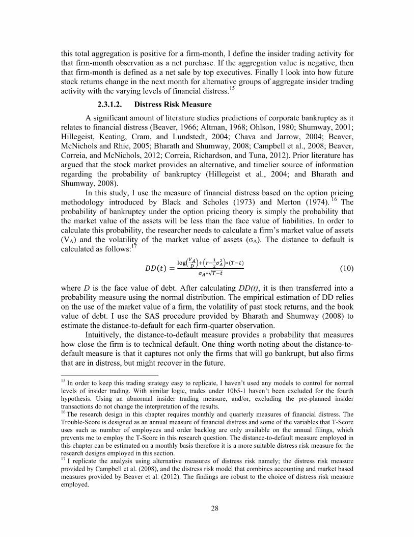
28

this total aggregation is positive for a firm-month, I define the insider trading activity for that firm-month observation as a net purchase. If the aggregation value is negative, then that firm-month is defined as a net sale by top executives. Finally I look into how future stock returns change in the next month for alternative groups of aggregate insider trading activity with the varying levels of financial distress.15

2.3.1.2. Distress Risk Measure

A significant amount of literature studies predictions of corporate bankruptcy as it relates to financial distress (Beaver, 1966; Altman, 1968; Ohlson, 1980; Shumway, 2001; Hillegeist, Keating, Cram, and Lundstedt, 2004; Chava and Jarrow, 2004; Beaver, McNichols and Rhie, 2005; Bharath and Shumway, 2008; Campbell et al., 2008; Beaver, Correia, and McNichols, 2012; Correia, Richardson, and Tuna, 2012). Prior literature has argued that the stock market provides an alternative, and timelier source of information regarding the probability of bankruptcy (Hillegeist et al., 2004; and Bharath and Shumway, 2008).

In this study, I use the measure of financial distress based on the option pricing methodology introduced by Black and Scholes (1973) and Merton (1974). 16 The probability of bankruptcy under the option pricing theory is simply the probability that the market value of the assets will be less than the face value of liabilities. In order to calculate this probability, the researcher needs to calculate a firm’s market value of assets (VA) and the volatility of the market value of assets (σA). The distance to default is calculated as follows:17

𝐷𝐷 𝑡 =£¤¥ ¦§

¨ # ��©ª«§ª ∗(¬�")

«§∗ ¬�" (10)

where D is the face value of debt. After calculating DD(t), it is then transferred into a probability measure using the normal distribution. The empirical estimation of DD relies on the use of the market value of a firm, the volatility of past stock returns, and the book value of debt. I use the SAS procedure provided by Bharath and Shumway (2008) to estimate the distance-to-default for each firm-quarter observation.

Intuitively, the distance-to-default measure provides a probability that measures how close the firm is to technical default. One thing worth noting about the distance-to-default measure is that it captures not only the firms that will go bankrupt, but also firms that are in distress, but might recover in the future. 15 In order to keep this trading strategy easy to replicate, I haven’t used any models to control for normal levels of insider trading. With similar logic, trades under 10b5-1 haven’t been excluded for the fourth hypothesis. Using an abnormal insider trading measure, and/or, excluding the pre-planned insider transactions do not change the interpretation of the results. 16 The research design in this chapter requires monthly and quarterly measures of financial distress. The Trouble-Score is designed as an annual measure of financial distress and some of the variables that T-Score uses such as number of employees and order backlog are only available on the annual filings, which prevents me to employ the T-Score in this research question. The distance-to-default measure employed in this chapter can be estimated on a monthly basis therefore it is a more suitable distress risk measure for the research designs employed in this section. 17 I replicate the analysis using alternative measures of distress risk namely; the distress risk measure provided by Campbell et al. (2008), and the distress risk model that combines accounting and market based measures provided by Beaver et al. (2012). The findings are robust to the choice of distress risk measure employed.

29

2.3.2. Research Design

In order to test the first hypothesis, I investigate the empirical association between the level of financial distress, insider trading, and accounting rates of return using quarterly cross-sectional regressions of the following form:

𝑃𝑒𝑟𝑓𝑜𝑟𝑚𝑎𝑛𝑐𝑒),�#$ = 𝛽� + 𝛽$𝑟𝑎𝑛𝑘(𝐷𝐷),�) + 𝛽R𝑟𝑎𝑛𝑘(𝐴𝑏. 𝐼𝑛𝑠𝑖𝑑𝑒𝑟𝑇𝑟𝑎𝑑𝑒𝑠),�) +𝛽N𝑟𝑎𝑛𝑘(𝐷𝐷),�) ∗ 𝑟𝑎𝑛𝑘(𝐴𝑏. 𝐼𝑛𝑠𝑖𝑑𝑒𝑟𝑇𝑟𝑎𝑑𝑒𝑠),�) + 𝛽U𝑋),�UI

U:E +𝜀� (11)

The dependent variable in Equation (11) is firm performance, proxied by return on equity (ROE) and return on asset (ROA). ROE is measured as the ratio of income before extraordinary items to the average value of shareholders’ equity, and ROA is measured as the ratio of income before extraordinary items, to the average value of total assets. The primary explanatory variables are the level of financial distress (DD), the level of abnormal insider trading, (Ab. Insider Trades) and their interaction. I use a quintile rank transformation for both of the explanatory variables. Specifically, firms are ranked quarterly and assigned to quintiles based on DD and Ab. Insider Trades, where the quarterly ranks are scaled to lie between 0.2 (lowest rank) and 1 (highest rank). This transformation mitigates potential non-linearity and makes the interpretation of the slope coefficient easier.

The vector of control variables Xk includes firm characteristics, which are known to be correlated with accounting rates of returns. These include the logarithm of total assets (AT), the book-to-market ratio (BM), quarterly percentage sales growth (SG), the profit margin (PM), the asset turnover ratio (A Turn) and leverage (Lev). The vector of control variables also controls for industry fixed effects based on two-digit SIC codes, due to their importance in cross-sectional variance in firm performance (Soliman, 2004). Quarter fixed effects are based on the calendar quarter of fiscal quarter ends, and are included to control for aggregate time varying factors affecting profitability measures and their decompositions. The estimations of standard errors are corrected for two-way clustering across time and firm.

In order to test the second hypothesis, I use a logit model for future performance related delistings, and seek to answer whether the information from insiders’ trades are providing incremental information over the existing distress risk measures and other variables known to be predictive for such events. The model I employ is as follows:

𝐼),�#$ = 𝛽� + 𝛽$𝐷𝐷),� + 𝛽R𝐴𝑏. 𝐼𝑛𝑠𝑖𝑑𝑒𝑟𝑇𝑟𝑎𝑑𝑒𝑠),� + 𝛽N𝑟𝑎𝑛𝑘(𝐷𝐷),�) + 𝛽E𝑟𝑎𝑛𝑘(𝐴𝑏. 𝐼𝑛𝑠𝑖𝑑𝑒𝑟𝑇𝑟𝑎𝑑𝑒𝑠),�) + 𝛽�𝑃𝑢𝑟𝑐ℎ𝑎𝑠𝑒),� + 𝛽�𝑆𝑒𝑙𝑙),� + 𝛽U𝑋),�UI

U:E +𝜀� (12)

The dependent variable in Equation (12) is an indicator variable that takes the value of one if a firm experiences a performance-related delisting during the following quarter (CRSP delisting codes 400 and codes between 550 and 585). DD is the distance-to-default measure, and Ab. Insider Trades is the residuals from Equation (9). Rank (DD) and rank (Ab. Insider Trades) are the quintile rank transformations of DD and Ab. Insider Trades respectively. Purchase (Sell) is an indicator variable that takes the value of one

30

when the rank of Ab. Insider Trades is one (zero), which classifies firm-quarter observations as being insider abnormal purchasers (abnormal sellers).

The vector of control variables Xk includes firm’s characteristics which are known to be predictive for bankruptcies and performance-related delistings, including logarithm of total assets (AT), the book-to-market ratio (BM), the volatility of past stock returns (SD), and an indicator variable for loss quarters. The vector of control variables also controls for industry fixed effects based on two-digit SIC codes, due to their importance in cross-sectional variance in bankruptcies (Chava and Jarrow, 2004) as well as their relevance in quarter fixed effects. The estimations of standard errors are corrected for two-way clustering across time and firm.

In the third hypothesis, I center on the association between investors’ reaction and the disclosure of top executives’ trades, and analyze how the level of financial distress affects this association. At the end of each month, I sort firms into quintiles based on their DD. I then examine the investors’ reaction to the disclosure of top executives’ trades, using the daily stock returns around the disclosure date for different quintiles of financial distress. 18 I use alternate windows surrounding the disclosure of insiders’ trades to understand whether there is a drift in investors’ reaction and/or a leakage of information prior to the disclosure.

I scrutinize investors’ reaction to the disclosure of top executives trades conditional on the level of financial distress, probing when firms are subject to higher levels of uncertainty, when there are greater information asymmetries, and when investors are paying more attention. I use size, bid-ask spread, trading volume, and volatility as proxies for uncertainty and information asymmetries, and I use the number of analysts following a firm, and the level of institutional ownership as proxies for investor attention. I then divide my sample into two, using each variable, and repeat the announcement return analyses using these subsamples for firms with the highest and lowest levels of financial distress.

For the final hypothesis, I sort firms into quintiles based on their level of financial distress at the beginning of each month. Then, I use a monthly aggregation period for the top executives’ transactions, as explained before. I classify firm month observations into two categories, with insiders as net sellers, and as net purchasers. These two criteria give me a total of 10 different portfolios for different financial distress risk levels, and different trading behaviors for top executives. The measures of distress risk and insider trading are calculated using the available information. In other words, all the variables are ex-ante available. I calculate the value-weighted monthly returns for each portfolio. Then, I regress the value weighted excess returns over the risk-free rate on a constant and on the market’s excess return (MKTRF), in addition to the standard Fama-French three-factor and four-factor models (Fama and French, 1993, 1996; Carhart, 1997). Finally I report the monthly alphas from these regressions with their t-statistics.

2.3.3. Sample and Data

My sample is taken from the intersection of the Compustat quarterly files (including the research file), the CRSP monthly returns file, the Thomson Reuters Insiders Data (TFN Insider Filing Data Files), and the Thomson Reuters Institutional 18 I use raw stock returns when I analyze the investors’ reaction. Adjusting the daily stock returns for market returns did not alter the interpretation of the results.

31

Holdings Database (13F), from January 1988 to December 2014. I focus on NYSE, AMEX and NASDAQ firms. I obtain raw stock returns from the CRSP Monthly Stock File and adjust for delisting returns following Beaver, McNichols, and Price (2007). My inferences remained the same when I did not adjust for delisting returns. I dropped financial companies (SIC 2-digit code between 60 and 65) and utility companies (SIC 2-digit code 49) from the sample. I further restrict my sample to firms with a share price greater than two dollars to assure that each stock has sufficient market liquidity, and that small, illiquid stocks do not drive the results. To reduce the impact of extreme observations, I trim financial variables at the top and the bottom one percentile based on quarterly cross-sectional cutoffs.

Table 10 provides descriptive statistics about the sample and the properties of the financial distress risk measure. Panel A depicts the summary statistics for the distance-to-default, insider trading variables, and other control variables for the full sample. For the entire sample the average firm had 8.4 percent probability of default based on distance-to-default, and the median firm had less than 0.1 percent probability of default. Panel B gives similar summary statistics for subsets of firm-quarter observations based on past aggregate trading activity. Sell presents the summary statistics for firms in which insiders were abnormal sellers in the previous quarter, and Purchase represents the firms in which insiders were abnormal purchasers. The firms in which top executives were purchasing more than usual, have a higher likelihood of default, lower future profits, ROE and ROA, and a higher frequency of reporting losses, compared to firms in which top executives were abnormal sellers.

Table 10, Panel C presents similar summary statistics for the breakdown of distress risk quintiles. The measure of abnormal insider trading activity (Ab. Insider Trades) monotonically increases with the level of financial distress. I also observe decreasing percentages of Sell with the level of financial distress, indicating the executives of financially distressed firms do not sell their stocks as much as the executives of financially healthy firms. Future profitability and size also decrease with the levels of financial distress, while book-to-market ratio and volatility of past stock returns, as well as the frequency of reporting losses, increases. All of these observed patterns are consistent with the prior literature.

Table 10, Panel C reveals additional information about financially distressed firms. The level of institutional ownership, and the average number of analysts following, decreases monotonically with the level of financial distress, indicating the less attention paid to financially distressed firms by investors. The amount of shares repurchased also decreases monotonically with the level of financial distress, and the most financially distressed firms on average, issue the least amount of new shares, confirming the argument that managers of financially distressed firms have limited tools with which to communicate their private information to the market.

2.4. Empirical Results

2.4.1. Top Executives’ Trades, Distress Risk, and Future Fundamental Firm Performance

In this section, I compare the relative informativeness of top executives’ trades for the future fundamental firm performance for firms with varying levels of financial

32

distress. More specifically, I examine the link between future accounting rates of return and top executives’ abnormal trading activity, and determine how the level of financial distress affects this link. I estimate quarterly cross-sectional regressions that are specified in Equation (11). The findings are presented in Table 11, where the first column reports the results when the dependent variable is Return on Equity (ROE). The main variables of interest are the interaction variable between the quintile rank transformation of the level of financial distress, and that of the abnormal trades by top executives. The first hypothesis predicts a positive coefficient for the interaction variable.

For the first model, where the dependent variable is ROE, the estimated coefficient on the rank (DD) is -0.1185 and significant at the one percent level. This finding implies that the ROE decreases by 11.85 percent from the least financially distressed firms to the most financially distressed firms. More interestingly, without controlling for the impact of the level of financial distress, I find a significant negative association between the future ROE and the level of abnormal trading by top executives. The coefficient on rank (Ab. Insider Trades) is significantly negative at 0.0132 indicating that when top executives abnormally purchase (sell) the firms tend to perform poorly (better) in the upcoming quarter. This negative association documented for the average firm could be associated with the fact that executives are opportunistically trading prior to performance reversals, using their insider knowledge of such events.

This negative association between future fundamental performance and top executives’ abnormal trades, switches sign however, once I control for the influence of financial distress. The coefficient on the interaction of rank (DD) and rank (Ab. Insider Trades) is 0.0225 and significant at one percent level. In other words, when managers of a financially distressed company purchase an abnormally large amount of shares, the ROE for the next quarter improves on average, by 2.25 percent. This coefficient is economically greater than the coefficient on rank (Ab. Insider Trades), negative 0.0132, indicating that the overall impact of excess trading by top executives in financially distressed firms, leads to improvements in ROE.

The mechanisms under discussion could be contributing to the documented improvement in the future accounting rate of return in financially distressed firms following top executives’ abnormal trades. One of the mechanisms in operation is the fact that managers of financially distressed firms are potentially more prone to litigation compared to managers of healthy firms. This being the case, managers are less likely to engage in opportunistic and misleading trades, which in turn leads to the positive coefficient documented for the interaction variables. In addition, the lack of other tools to communicate their private information during times of financial distress, could force management to use their personal trades as a signaling device. If this is the case, their trades should reflect the true nature of the business. Therefore it is normal to observe a positive association between the abnormal trading activity and the future accounting rates of return, after controlling for the impact of financial distress.

The second column of Table 11, repeats the model provided by Equation (11) and uses the Return on Asset (ROA) as the dependent variable. The results are very similar to column one. There is a significant negative association between the level of financial distress and future profitability, and a significant negative association between top executives’ abnormal trades and future ROA. The coefficient on the interaction of rank (DD) and rank (Ab. Insider Trades) is 0.0105 and significant at one percent level. This

33

finding shows that the documented relationship holds for an alternative measure of accounting rate of return, and thus provides additional proof for the first hypothesis.

The next three columns on Table 11 present the results for the components of ROA and ROE in the DuPont framework. Profit margin (PM), asset turnover (A_Turn), and financial leverage (Lev) are the dependent variables for column three, four, and five respectively. The coefficient on rank (DD) is negative for profit margin and asset turnover, while it is positive for the financial leverage. The coefficient on rank (Ab. Insider Trades) is significantly negative for profit margin, and significantly positive for financial leverage. The coefficient on the interaction of rank (DD) and rank (Ab. Insider Trades) is slightly significantly positive for PM, significantly positive for A_Turn, and significantly negative for Lev. This indicates that when managers of financially distressed firms purchase an abnormally large amount of shares, the future profit margin, asset turnover and capital structure of the firm improves. This additional evidence enhances our understanding of the documented positive association between future accounting rates of return and the interaction of rank (DD) and rank (Ab. Insider Trades). The increased profitability mainly comes through the improvement in the capital structure of the firm and through increased utilization of existing assets. The weak improvement in profit margin also contributes to the enhanced informativeness.

2.4.2. Top Executives’ Trades and Performance Related Delistings

In order to understand whether insiders’ trades are informative about the likely survival of firms, I estimate the logit model specified in Equation (12). The results are presented in Table 12. The first column uses the raw values of the distance-to-default (DD) measure, as well as my measure of abnormal insider trading (Ab. Insider Trades). As expected, DD is significantly positive at one percent level. The estimate of the coefficient for Ab. Insider Trades is significantly negative at five percent level. This finding reveals that on average, abnormal trading activity increases the likelihood of survival.

In column two of Table 12, I replace the raw values of DD and Ab. Insider Trades with their quintile rank transformations. The results are similar to the first column. The only improvement is the significance of the coefficient on rank (Ab.Insider Trades), which in column two is significant at one percent level. The final column of Table 12 investigates the impact of top executives’ abnormal purchases and abnormal sales, considering each separately to address part a and part b of the second hypothesis. The variable Purchase, an indicator variable for the abnormal purchases of top executives, has a significantly negative coefficient, which implies that top executives’ purchases decrease the likelihood of a performance related delisting. More to the point, I document a significant negative coefficient on the indicator variable for top executives’ abnormal selling. This finding implies that managers’ excessive selling decreases the likelihood of performance related delistings. This finding is consistent with the literature that shows that, in order to avoid litigation, managers avoid selling their own company’s shares prior to declaring bankruptcy (Gosnell et al., 1992). The findings in this section provide strong support for the second hypothesis.

34

2.4.3. Investors Reaction to Disclosure of Top Executives’ Trades

In this section I analyze investors’ reaction to the disclosure of top executives’ trades in firms with varying levels of financial distress, as measured by announcement window returns. I use four alternative event windows to measure the investors’ reaction. For each distress risk quintile following insiders’ purchases and sales, I report the average return, the mean and median return, as well as the frequency of positive returns for alternative holding periods in Table 13. Figure 7 plots the average daily returns for two-days on either side of the executives’ trades, conditional on the level of distress risk for the firms. The magnitude of the reaction is greater for the most financially distressed firms.

I begin by looking at the day zero returns, the returns on the day that insiders’ trades are disclosed to SEC. When insiders purchase in a financially healthy firm, there is a positive reaction of 0.209 percent. The average announcement day return for financially distressed firms is 0.562 percent, and there is a monotonic increase in the average reaction with the level of financial distress. The median returns are zero regardless of the level of financial distress. Even though I fail to observe a trend in returns following insiders’ sales that correlates with the level of financial distress, the most negative reaction is negative 0.161 percent for the most financially distressed firms.

The second return window I examine includes the previous day, the announcement day, and the day after the disclosure of the insiders’ trades. The three-day return for the most financially distressed firms is 1.82 percent, while the median return for the same group is 0.644 percent. Following top executive’s purchases 55 percent of the observations have a positive cumulative return in financially distressed firms. There is a monotonic increase in the median returns, and an almost monotonic increase in the average returns with the level of financial distress following insiders’ purchases. The most negative reaction to insiders’ sales occurs in the financially distressed firms with a negative 0.450 percent cumulative return, and only 46 percent of the returns for this group are greater than zero.

Third, I analyze the cumulative returns for the two-day period including the announcement day of the top executives’ trades, and the day after. The average return following insiders’ purchases is greatest for the most financially distressed firms, and there is a monotonic increase in the returns associated with the level of financial distress. The average return for the most financially distressed firms is 1.504 percent, which is slightly lower than the 1.820 percent reported for the three-day event window that includes the day before the announcement. This indicates that there could be some leakage of information prior to the disclosure of the announcement of the managers’ trades. The results for the sales are similar; the most negative reaction takes place in the most financially distressed firms.

Finally, I look at the three-day cumulative return including the announcement day return, and two-days after the announcement. The average return following an announcement of insiders’ purchases is 2.086 percent for the most financially distressed firms. This number is 50 basis points greater than the return for the two-day event window that includes the announcement day and the day after the announcement. This difference suggests that there is a small drift in stock returns. There is a monotonic relationship between the median returns and the level of financial distress following managers’ purchases, and an almost monotonic relationship between the average returns

35

and the level of financial distress. The results for sales are similar to the alternative event windows. Investors react most negatively to executives’ selling of stock in the most financially distressed firms.

The results presented in this section provide strong evidence for the third hypothesis. Investors’ reaction to the disclosure of top executives’ purchases increases with the level of financial distress regardless of the event-window. And investors also react most negatively to the disclosure of sales by top executives when the firm is financially distressed.

2.4.3.1. Uncertainty, Asymmetry, Investor Attention and Investors Reaction to Disclosure of Top Executives’ Trades

In this section I focus on investors’ reaction to the disclosure of top executives’ trades in the most and least financially distressed firms. The analysis is carried out across subsamples based on variables that are proxies for uncertainty, information asymmetry, and investor attention. I sort firms into quintiles based on their level of financial distress at the end of the month before the disclosure of the top executives’ trades. Then I focus on the three-day cumulative return, including the announcement day return, and the return two days after the announcement.

I use size, bid-ask spread, trading volume, and volatility as proxies for uncertainty and information asymmetries. In addition, I use the number of analysts following a firm, and the level of institutional ownership as proxies for investor attention. Based on these variables, I form subsamples and examine investors’ reaction to the disclosure of top executives’ trades in financially distressed firms and healthy firms across those subsamples.

Investors’ reaction to the disclosure of top executives’ trades could be different when firms are subject to higher levels of uncertainty and larger information asymmetries, or when they experience greater attention from investors. The presence of financial distress is positively correlated with uncertainty and information asymmetry, and negatively correlated with investor attention. Therefore the documented increase in the investors’ reaction to the disclosure of top executives’ trades, given different levels of financial distress, could be driven by these factors and not by the level of distress. The analyses of the subsamples verify that the documented increase is indeed caused by the level of financial distress, and not by uncertainty, information asymmetry or investor attention.

Here I begin by analyzing the difference in investors’ reaction for small versus big firms. Size, the logarithm of the market capitalization of firms, has been used to proxy for uncertainty, information asymmetry, and the level of investor attention in previous literature. The results presented in Table 14 show that reaction to investors’ purchases are bigger for smaller firms, independent of the level of financial distress. In addition, regardless of the level of size, there is always a statistically significant and economically meaningful difference in the investors’ reaction to the disclosure of top executives’ purchases for both financially distressed firms and healthy firms in the predicted direction. In the presence of financial distress, investors seem to react more negatively to the disclosure of top executives’ sales when the firms are bigger. This can be explained by the attention story; management selling behavior in a bigger firm garners more attention from the market compared to management selling behavior in a smaller firm.

36

Bid-ask, volume, and volatility subsamples give rise to an almost identical result. High bid-ask spread, high volume, and high volatility are associated with higher levels of both uncertainty and information asymmetry. In the presence of high uncertainty and high information asymmetry, the release of new information to the market has the potential to create a bigger reaction (Zhang, 2006). Consistent with this, I find for both purchases and sales, the top executives’ trades create a bigger reaction in the presence of high uncertainty and information asymmetry. Regardless of the subsample, I observe a greater reaction to the disclosure of top executives’ trades if the firms are experiencing financial difficulties.

Finally, I look at the number of analysts following, and the level of institutional ownership. If there is higher investor attention, I anticipate finding a bigger reaction to the disclosure of top executives’ trades. Consistent with this expectation, I find the reaction to top executives’ purchases is 4.17 percent when there is a high number of analysts following a distressed firm – a full 1.77 percentage points higher than investor reaction when there is a low number of analysts following the firm. Similarly, when the level of institutional ownership is higher, the reaction to the disclosure of top executives’ trades in financially distressed firms is 3.15 percent, a figure that is 50 percent higher than the reaction when the level of institutional ownership is lower. The results for the top executives’ sales are similar; there is a bigger reaction to the disclosure of top executives’ sales when there is more attention paid to firms.

The results in this section show that the reaction to the disclosure of top executives’ trades are bigger when there is higher investor attention, and when the firm is surrounded by uncertainty or information asymmetry. The results also support the third hypothesis, that no matter which subsample is used, the reaction to the disclosure of top executives’ trades is significantly greater when a firm is financially distressed compared to when a firm is financially healthy.

2.4.4. Future Returns to Aggregate Insider Trading conditional on Financial Distress

In Table 15, I evaluate the final hypothesis by analyzing returns following the two types of aggregate insider trading activity (net purchasers or net sellers), conditional on the level of financial distress. For each sub-group of firms, I calculate the value weighted one-month ahead future returns for each quarter.19 I then regress the excess returns of portfolios over the risk-free rate on a constant, the market’s excess return (MKTRF), and the three-factor and four-factor models based on the Fama-French factors (HML, SMB, UMD). I report the monthly alphas and t-statistics from these regressions.

Panel A of Table 15 reports the excess future returns for the firm month observations in which insiders were net sellers in the prior month. I fail to find any significant future returns in the next month for the most financially distressed firms. It is possible for such firms that the price formation had already taken place prior to the portfolio formation date. I also fail to observe any patterns in the excess future returns following top executives’ sales with the level of financial distress. The future returns of 19 The interpretation of the results remains unchanged, when portfolios are formed using equal weights. I observe a stronger negative trend in future abnormal returns for firms in which insiders are net sellers. I also observe an increase in the magnitude of future abnormal earnings for firms in which insiders are net purchasers.

37

the firms that are in the fourth quintile based on their financial distress in the previous month, however, have significantly negative abnormal returns when CAPM and 3-factor models are used. The average investor reaction to the disclosure of top executives’ sales for firms in the fourth quintile based on their level of financial distress in the previous month, is positive for three out of four return windows as presented in Table 13. It can be concluded that there is a potential drift in stock returns for this group.20

In Panel B, I analyze the excess monthly future stock returns following top executives’ purchasers. Regardless of the excess return measure, I observe a monotonic increase in the excess stock returns with the level of financial distress. This evidence shows that there is a bigger drift in future stock returns if the firms are experiencing financial difficulties. The monthly excess returns for the most financially distressed firms range between 1.43 and 2.08 percent (18.6 and 28 percent annualized returns respectively). In Figure 8, I plot the monthly excess returns using the four-factor model. Two hundred out of 323 observations, or 62 percent, are positive. The most positive return took place in January 2005 with 45.7 percent, and the most negative return was in May 2011 with negative 29.4 percent.

The evidence presented in this section partially supports the final hypothesis. Following insiders’ sales, the drift seems not to exist, at least not in a systematic way. Following top executives’ sales, however, the magnitude of the excess returns, as well as their significance, increases with the level of financial distress. This finding indicates that investors do not fully incorporate the predictive content of top executives’ purchases in financially distressed firms.

2.4.4.1. Uncertainty, Asymmetry, Investor Attention and Future Returns for Financially Distressed Firms in Which Top Executives’ Were Net Purchasers

Similar to the analyses in Section 4.3.1, I perform subsample analyses for the excess future stock returns for financially distressed firms in which top executives’ were net purchasers in the previous month. I focus on purchases because there was no significant drift following top executives’ sales. I report the value-weighted monthly excess returns using the four-factor model for each portfolio. The results are presented in Table 16.

The drift in stock returns is larger if the firms are small, a finding consistent with the gradual-information diffusion model of Hong and Stein (1999). The drift is smaller when firms have higher bid-ask spreads, past trading volume, and volatility, consistent with the fact that the initial reaction to the announcement of top executives’ purchases was higher for these subsamples. Table 14 showed that in these subsamples the average returns around the disclosure date were smaller. The excess returns for these subsamples are still significant at one percent level. Of note is the fact that in the high analyst following sample, I fail to find a significantly positive future stock return. In addition, the presence of high institutional ownership reduces the monthly average excess returns from 2.67 percent to 1.64 percent, a reduction of 13.1 percent when annualized. This shows

20 In untabulated results, I also analyzed the future excess returns for firm-month observations when top executives did not engage in trading in the previous month. I failed to observe any patterns in these excess returns across levels of financial distress.

38

that when there is higher attention paid by investors, the drift in future stock returns is smaller, or non-existent.

2.5. Concluding Remarks

This chapter examines the information content of top executives’ trades for future performance, and compares the informativeness of such trades in financially distressed firms to that of financially healthy firms. The results indicate a negative association between top executives’ abnormal trading activity and the future accounting rates of return when one does not control for the level of financial distress. That association becomes significantly positive however, after controlling for the level of financial distress suggesting that top executives’ trades are better aligned with future fundamental performance for firms experiencing financial distress.

The results of the logit models for predicting performance related delistings indicate that the insiders possess private information about the likelihood of survival. I show that, on average, abnormal trades by top executives increase the likelihood of survival. I find that firms are less likely to get delisted following abnormal purchases of top executives. In addition, the findings imply that managers’ excessive selling decreases the likelihood of performance related delistings. I interpret the latter evidence as managers avoid selling prior to delistings in order to limit their exposure to litigations and reduce their reputational risks.

The tests of investors’ reaction to the disclosure of top executives’ trades, measured by announcement day returns, reveal that such trades are more informative in the presence of financial distress. The magnitude of the returns surrounding the top executives’ purchases, increases with the level of financial distress. I also find that the investors’ reaction to the top executives’ sales is most negative for the financially distressed firms. I measure the level of investor attention by number of analysts following and the level of institutional ownership. I find that the the magnitude of the reaction to top executives’ trades is larger when the investor attention is high.

Finally, I document a delay in price formation following top executives’ purchases. Future abnormal returns for firms in which top executives were net purchasers in the previous month, increases monotonically with the level of financial distress. My findings suggest that investors do incorporate some, but not all of the information content revealed by top executives’ trades in financially distressed firms. I also find that the drift is smaller or non-existent in firms where there is a higher attention paid by market participants. This evidence suggests that among the firms which attract relatively less attention from market participants, investors treat the top executives’ trades in financially distressed firms in a similar manner the top executives’ trades within healthier firms, leading to delayed price formations.

39

Bibliography Abarbanell, J. S. and B. J. Bushee, 1998. Abnormal Returns to a Fundamental Analysis

Strategy. The Accounting Review 73, 19–45.

Aboody, D., Lev, B., 2000. Information Asymmetry, R&D, and Insider Gains. The Journal of Finance 55 (26), 2747-2766.

Aboody, D., Hughes, J., Liu, J., 2005. Earnings Quality, Insider Trading, and Cost of Capital. Journal of Accounting Research 44 (5), 651-673.

Ak, B. K., Dechow, P. M., Sun, Y., Wang, A. Y., 2013. The use of financial ratio models to help investors predict and interpret significant corporate events. Australian Journal of Management 38 (3), 553-598.

Ak, B. K., Rossi, B., Sloan, R., Tracy, S., 2016. Navigating Stock Price Crashes. Journal of Portfolio Management, forthcoming.

Altman, E. I., 1968. Financial ratios, discriminant analysis and the prediction of corporate bankruptcy. The Journal of Finance 23 (4), 589-609.

Basu, S., 1997. The conservatism principle and the asymmetric timeliness of earnings. Journal of Accounting and Economics 24 (1), 3-37.

Beaver, W. H., 1966. Financial ratios as predictors of failure. Journal of Accounting Research 4, 71-111.

Beaver, W. H., Correia, M., McNichols, M. F., 2012. Do differences in financial reporting attributes impair the predictive ability of financial ratios for bankruptcy? Review of Accounting Studies 17 (4), 969-1010.

Beaver, W. H., McNichols, M., Price, R., 2007. Delisting returns and their effect on accounting-based market anomalies. Journal of Accounting and Economics 43 (2), 341-368.

Beaver, W. H., McNichols, M. F., Rhie, J.-W., 2005. Have financial statements become less informative? Evidence from the ability of financial ratios to predict bankruptcy. Review of Accounting Studies 10 (1), 93-122.

Beneish, M. D., Lee, C. M., Tarpley, R. L., 2001. Contextual fundamental analysis through the prediction of extreme returns. Review of Accounting Studies 6 (2-3), 165-189.

Beneish, M. D., Press, E., Vargus, M. E., (2012). Insider Trading and Earnings Management in Distressed Firms. Contemporary Accounting Research 29 (1). 191-220.

Beneish, M., and Vargus, M. (2002). Insider trading, earnings quality, and accruals mispricing. The Accounting Review 77(4), 755–791.

Bettis, C., Vickrey, D., Vickrey, D. W., 1997. Mimickers of corporate insiders who make large-volume trades. Financial Analysts Journal 53 (5), 57-66.

40

Bharath, S. T., Shumway, T., 2008. Forecasting default with the Merton distance to default model. Review of Financial Studies 21 (3), 1339-1369.

Black, F., Scholes, M., 1973. The pricing of options and corporate liabilities. The Journal of Political Economy 81 (3), 637-654.

Bradshaw, M. T., Richardson, S. A., Sloan, R. G., 2006. The relation between corporate financing activities, analysts’ forecasts and stock returns. Journal of Accounting and Economics 42 (1), 53-85.

Campbell, J. Y., Hilscher, J., Szilagyi, J., 2008. In search of distress risk. The Journal of Finance 63 (6), 2899-2939.

Carhart, M. M., 1997. On persistence in mutual fund performance. The Journal of Finance 52 (1), 57-82

Chava, S., Jarrow, R. A., 2004. Bankruptcy prediction with industry effects. Review of Finance 8 (4), 537-569.

Charitou, A., Lambertides, N. Trigeorgis, L., 2007. Earnings Behaviour of Financially Distressed Firms: The Role of Institutional Ownership. Abacus 43(3), 271-296.

Chen, C., Martin, X., Wang, X., 2013. Insider Trading, Litigation Concerns, and Auditor Going-Concern Opinions. The Accounting Review 88 (2), 365-393.

Cheng, Q., Lo, A. K., 2006. Insider Trading and Voluntary Disclosures. Journal of Accounting Research 44 (5), 815-848.

Cohen, L., Malloy, C., Pomorski, L., 2012. Decoding Insider Information. The Journal of Finance 67 (3), 1009-1043.

Core, J. E., Guay, W. R., Richardson, S., Verdi, R., 2006. Stock market anomalies: what can we learn from repurchases and insider trading? Review of Accounting Studies 11 (1), 49–70.

Correia, M., Richardson, S. A., Tuna, I., 2012. Value investing in credit markets. Review of Accounting Studies 17 (3), 572-609.

Dambolena, I. G. and S. J. Khoury. 1980. Ratio stability and corporate failure. The Journal of Finance 35 (4), 1017-1026.

De Bondt, W. F., Thaler, R., 1985. Does the stock market overreact? The Journal of Finance 40 (3), 793-805.

Dechow, P. M., Ge, W., Larson, C. R., Sloan, R. G., 2011. Predicting material accounting misstatements. Contemporary Accounting Research 28 (1), 17-82.

Dichev, I. D., 1998. Is the risk of bankruptcy a systematic risk? The Journal of Finance 53 (3), 1131-1147.

Fama, E. F., French, K. R., 1993. Common risk factors in the returns on stocks and bonds. Journal of Financial Economics 33 (1), 3-56.

Fama, E. F., French, K. R., 1996. Multifactor explanations of asset pricing anomalies. The Journal of Finance 51 (1), 55-84.

41

Fama, E. F., MacBeth, J. D., 1973. Risk, return, and equilibrium: Empirical tests. The Journal of Political Economy 81 (3), 607-636.

Frankel, R., Li, X., 2004. Characteristics of a firm’s information environment and the information asymmetry between insiders and outsiders. Journal of Accounting and Economics 37 (2), 229-259.

Frost, C. A., 1997. Disclosure policy choices of UK firms receiving modified audit reports. Journal of Accounting and Economics 23 (2), 163-187.

Garlappi, L., Shu, T., Yan, H., 2008. Default risk, shareholder advantage, and stock returns. Review of Financial Studies 21 (6), 2743-2778.

Gosnell, T., Keown, A. J., Pinkerton, J. M., 1992. Bankruptcy and insider trading: Differences between exchange-listed and OTC firms. The Journal of Finance 47 (1), 349-362.

Griffin, P. A., Lont, D. A., McCulne, K. (2014). Insightful Insiders? Insider Trading and Stock Return around Debt Covenant Violation Disclosures. Abacus 50 (2), 117-145.

Hayn, C., 1995. The information content of losses. Journal of Accounting and Economics 20 (2), 125-153.

Hillegeist, S. A., Keating, E. K., Cram, D. P., Lundstedt, K. G., 2004. Assessing the probability of bankruptcy. Review of Accounting Studies 9 (1), 5-34.

Holthausen, R. W., Larcker, D. F., 1992. The prediction of stock returns using financial statement information. Journal of Accounting and Economics 15 (2), 373-411.

Hong, H., Stein, J. C., 1999. A Unified Theory of Underreaction, Momentum Trading, and Overreaction in Asset Markets. The Journal of Finance 54 (6), 2143-2184.

Hutton, A. P., Marcus, A. J., Tehranian, H., 2009. Opaque financial reports, R2, and crash risk. Journal of Financial Economics 94 (1), 67-86.

Jagolinzer, A. D., 2009. SEC Rule 10b5-1 and Insiders' Strategic Trade. Management Science 55 (2), 224-239.

Jagolinzer, A. D., Larcker, D. F., Taylor, D. J., 2011. Corporate Governance and the Information Content of Insider Trades. Journal of Accounting Research 49 (5), 1249-1274.

Jegadeesh, N., Titman, S., 1993. Returns to buying winners and selling losers: Implications for stock market efficiency. The Journal of Finance 48 (1), 65-91.

Karpoff, J. M., Lee, D., 1991. Insider Trading before New Issue Announcements. Financial Management 20 (1), 18-26.

Ke, B., Huddart, S., Petroni, K., 2003. What insiders know about future earnings and how they use it: Evidence from insider trades. Journal of Accounting and Economics 35 (3), 315-346.

Lakonishok, J., Lee, I., 2001. Are insider trades informative? Review of Financial Studies 14 (1), 79-11.

42

Lee, D. S., Mikkelson, W. H., Partch, M. M., 1992. Managers' Trading Around Stock Repurchases. The Journal of Finance 47 (5), 1947-1961.

Lee, I., 1997. Do Firms Knowingly Sell Overvalued Equity? The Journal of Finance 52 (4), 1439-1466.

Leland, H. E., Pyle, D. H., 1977. Information Asymmetries, Financial Structure, and the Intermediation. The Journal of Finance 32 (2), 371–387.

Lev, B. and R. Thiagarajan. (1993). Fundamental Information Analysis. Journal of Accounting Research 31 (2), 190–202.

Loderer, C. F., Sheehan, D. P., 1989. Corporate Bankruptcy and Managers' Self-Serving Behavior. The Journal of Finance 44 (4), 1059-1075.

Ma, Y., 2001. Insider trading behavior prior to chapter 11 bankruptcy announcements. The Journal of Business Research 54 (1), 63-70.

Merton, R. C., 1974. On the pricing of corporate debt: The risk structure of interest rates. The Journal of Finance 29 (2), 449-470.

Morton, R. M., Shane, P. B., 1998. The information environment and the ability of logit-based financial statement analysis to predict abnormal returns. Accounting & Finance 38 (1), 71-89.

Ohlson, J. A., 1980. Financial ratios and the probabilistic prediction of bankruptcy. Journal of Accounting Research 18 (1), 109-131.

Ou, J. A., Penman, S. H., 1989. Financial statement analysis and the prediction of stock returns. Journal of Accounting and Economics 11 (4), 295-329.

Piotroski, J. D., 2000. Value investing: The use of historical financial statement information to separate winners from losers. Journal of Accounting Research 38, 1-41.

Piotroski, J. D., Roulstone, D. T., 2005. Do insider trades reflect both contrarian beliefs and superior knowledge about future cash flow realizations? Journal of Accounting and Economics 39 (1), 55-81.

Rozeff, M. S., and M. A. Zaman, 1988, Market Efficiency and Insider Trading: New Evidence, The Journal of Business, 61 (1), 25-44.

Rozeff, M. S., and M. A. Zaman, 1998, Overreaction and Insider Trading: Evidence from Growth and Value Portfolios, The Journal of Finance, 53 (2), 701-716.

Seyhun, H. N., 1986. Insiders' profits, costs of trading, and market efficiency. Journal of Financial Economics 16 (2), 189-212.

Seyhun, H. N., 1988. The information content of aggregate insider trading. The Journal of Business 61 (1), 1-24.

Seyhun, H. N., 1992. Why does aggregate insider trading predict future stock returns? The Quarterly Journal of Economics 107 (4), 1303-1331.

43

Seyhun, H. N., Bradley, M., 1997. Corporate bankruptcy and insider trading. The Journal of Business 70 (2), 189-216.

Shumway, T., 2001. Forecasting bankruptcy more accurately: A simple hazard model. The Journal of Business 74 (1), 101-124.

Skinner, D. J., 1994. Why Firms Voluntarily Disclose Bad News. Journal of Accounting Research 32 (1), 38-60.

Skinner, D. J., Sloan, R. G., 2002. Earnings surprises, growth expectations, and stock returns or don’t let an earnings torpedo sink your portfolio. Review of Accounting Studies 7 (2-3), 289-312.

Sloan, R. G., 1996. Do stock prices fully reflect information in accruals and cash flows about future earnings? The Accounting Review 71 (3), 289-315.

Soliman, M. T., 2004. Using industry-adjusted DuPont analysis to predict future profitability. Ph.D. Dissertation, University of Michigan.

Soliman, M. T., 2008. The use of DuPont Analysis by Market Participants. The Accounting Review 83 (3), 823-853.

Tavakoli, M., McMillan, D., McKnight, P. J., 2012. Insider trading and stock prices. International Review of Economics & Finance 22 (1), 254-266.

Veenman, D., 2012. Disclosures of Insider Purchases and the Valuation Implications of Past Earnings Signals. The Accounting Review 87 (1), 313-342.

Vermaelen, T., 1981. Common Stock Repurchases and Market Signaling. Journal of Financial Economics 9 (2), 139–183.

Watts, R. L., 2003a. Conservatism in accounting part I: Explanations and implications. Accounting Horizons 17 (3), 207-221.

Watts, R. L., 2003b. Conservatism in accounting part II: evidence and research opportunities. Accounting Horizons 17 (4), 287-301.

Yur-Austin, J., 1998. Can insiders bail themselves out before private renegotiation? Review of Financial Economics 7 (2), 197-211.

Zhang, X. F., 2006. Information Uncertainty and Stock Returns. The Journal of Finance 61 (1), 105-137.

44

Exhibit 1: Variable Descriptions Leverage / Liquidity FL Financial Leverage, Total liabilities (lt) divided by total assets (at). OL Operating Leverage, Cost of Goods Sold (cogs) divided by Cost of Goods Sold

plus the Selling, General, and Administrative Expenses (xsga). WCTA Working Capital to Total Assets, Working Capital (Current Assets (act) -

Current Liabilities (lct)) divided by total assets. ICR Interest Coverage Ratio, Operating Income (oiadp) divided by the Interest

Expense (xint). CR Current Ratio, Current Assets (act) divided by Current Liabilities (lct). ΔFL Change in Financial Leverage, % Change in Financial Leverage (FL) over the

previous year. Performance ROA Return on Assets, Net Income (ib) divided by Total Assets (at). ETL EBITDA (oibdp) to Total Liabilities (lt) NEG An indicator variable that takes the value of one if net income (ib) is negative

for the year. RET Annual stock return during the previous year. RET_3 Previous three-year cumulative stock return CCC Cash Conversion Cycle, Average Inventory (invt) / (Cost of Goods Sold (cogs)

/365)+ Average Receivables (rect) /(sale/365)- Average Accounts Payable (ap) /(cogs/365)

AB.EMP Abnormal Change in Employee, Percentage change in the number of employees (emp) minus percentage change in assets (at).

AB.OB Abnormal Change in Order Backlog, Percentage change in order backlog (ob) minus percentage change in sales (sale).

ΔROA Change in ROA, % Change in Return on Assets (E/P) over the previous year Turnover A.TURN Asset Turnover Ratio, Sales (sale) scaled by Total Assets (at). ΔA.TURN Change in Asset Turnover, % Change in Asset Turnover (A.TURN) over the

previous year. INV.TURN Inventory Turnover Ratio, Cost of Goods Sold (cogs) divided by Average

Inventory (invt) ΔINV.TURN Change in Inventory Turnover, % Change in Inventory Turnover (INV.TURN)

over the previous year. Volatility SD The standard deviation of the last 12 month stock returns. VOLUME The difference between the trading volume during the month prior to the

portfolio formation and the average trading volume for the previous 11 month period scaled by the standard deviation of trading volume during the same period.

BID_ASK The difference between the bid-ask spread during the month prior to the portfolio formation and the average bid-ask spread for the previous 11 month period scaled by the standard deviation of bid-ask spread during the same period.

SD_SALE The standard deviation of sales (sale) scaled by total assets using previous three annual observations.2

SD_NI The standard deviation of net income (ib) scaled by total assets using previous three annual observations. 2

SD_CF The standard deviation of cash flow (ib - acc) scaled by total assets using previous three annual observations. 2, 3

SIZE Logarithm of Market Value of Equity.

45

FS Quality ACC/TA Accruals to Total Assets, ((ΔCurrent Assets (act) – ΔCash and Short-term

Investments (che))– (ΔCurrent Liabilities (lct) – ΔDebt in Current Liabilities (dlc) – ΔTaxes Payable (txp)) ⁄ Average total assets.

ACC.IND Abnormal Accruals, An indicator variable that takes the value of one if the absolute value of total accruals fells into top 90 percentile.

%SA % of Soft Assets, (Total Assets (at) - PP&E (ppent) – Cash and Cash Equivalent (che)) scaled by Total Assets (at).

Torpedo BtoM Book-to-Market Ratio, Book Value of Equity (ceq) divided by Market

Capitalization. E/P Earnings-to-Price Ratio, Earnings Per Share (epsfx) divided by Price. ΔEQUITY The net cash received from the sale (and/or purchase) of common and

preferred stock less cash dividends paid (sstk - prstkc - dv, based on Bradshaw, Richardson, and Sloan, 2006).

SHORT The shares held (adjusted) short as of settlement date provided by Compustat divided by common shares outstanding.

SG Sales Growth, % Change in Total Sales (sale) over the year. ΔE/P Change in Earnings-to-Price Ratio, % Change in Earnings-to-Price Ratio

(E/P) over the previous year DECLINE_SALES An indicator variable that takes the value of one if the sales decline over

the previous year. CAPEX Capital Expenditure to Total Assets, Capital Expenditure (capx) divided by

Total Assets (at) Other NEG_SD An interaction variable between the indicator variable for negative net

income (NEG) and the standard deviation of past stock returns. NEG_SD_NI An interaction variable between the indicator variable for negative net

income (NEG) and the standard deviation of net income. RD Research and Development Expense (xrd) scaled by Sales (sale). I An indicator variable, which takes the value of one when the one-year

ahead stock return of a company falls into the bottom five percentile of stock returns for the given year.

T Trouble Score (T-Score) Z Altman Z-Score B Distress risk measure calculated using the variables and coefficients in

Beaver et al. (2012) C Distress risk measure calculated using the variables and coefficients in

Campbell et al. (2008) DD Distress risk measure based on Black and Scholes (1973) and Merton

(1974) estimated using the SAS procedure provided by Shumway (2001). P Pitoroski (2000) Score

1 All the explanatory variables expect Standard deviation of past stock returns (SD) are trimmed from bottom and top at 1% annual cross-sectional cutoffs. 2 I also used five years to calculate the standard deviation of the measures instead of three years, the variables were highly correlated, in order not to place too much demand on the data, I preferred to choose the standard deviations using three years. The inferences are not changed if I used the standard deviations calculated using the observations from previous five years. 3 Cash Flow is calculated as the difference between net income (ib) and the total accruals (acc) is the variable calculated for the variable Acc/TA. 4 The variable names for the Compustat database are provided in parenthesis next to the related variable.

46

Exhibit 2: Explanatory variables that have been used in the prior literature Study

Leverage/Liquidity Performance Turnover Volatility FS

Quality Torpedo Beaver (1966) TL/TA

WC/TA CA/CL

CFO/TL ROA

Altman (1968) ME/TL RE/TA EBIT/TA

SALES/TA

Ohlson(1980) CL/TA NEG. ROA ΔROA NEG. EQUITY

ln(TA/GNP price-level index)

Dambolena and Khoury (1980)

CL/BE σ(CL/BE)1 σ(TL/TA) σ(ROE)

Shumway (2001) RET LSIGMA Beaver, McNichols, and Rhie (2005)

EBITDA/TL SIZE

Campbell, Hilscher, and Szilagyi (2008)

TL/MTA2

CHE/MTA2 NI/MTA3 PRICE MtoB

Beaver, Correia, McNichols (2012)

NEG.ROA*TL/TA NEG.ROA*EBITDA/TL

NEG.ROA*ROA NEG.ROA*LERET

NEG.ROA*Ln(ME) NEG.ROA*LSIGMA

Trouble-Score OL ΔFL ICR

RET_3 CCC AB.EMP AB.OB ΔROA

ΔA.TURN INV.TURN ΔINV.TURN

σ(SALES/TA) σ(NI/TA) σ(CFO/TA) NEG.ROA*σ(NI/TA) VOL BID_ASK

ACC/TA ACC.IND %SA

SHORT E/P ΔE/P ΔEQUITY SG DECLINE_SALES CAPEX

Market variables are identified in bold and italic. 1 In the paper, the authors use the term "Net Worth" for the denominator, however I failed to find a description of it. I believe it to be the "Book Value of Equity (BE)". 2 MTA is total assets adjusted: for the market value of equity MTA = TA + 0.1(ME-BE). The articles listed in this Exhibit does not cover all the papers that studied the prediction of bankruptcy. The list consists of papers that offered a new explanatory variable that has information content for predicting bankruptcies.

47

Figure 1 – Frequency of 50 percent or more stock price declines by year

This figure plots the number of 50 percent or more stock price declines over the subsequent years for the 1971-2012 period.

Figure 2– Monthly Stock Returns of Extreme-Decline Firms and Other Firms

This figures shows the average monthly stock returns for the firms identified as firms that experience 50 percent or more stock price decline and the all the other firms. The average monthly raw returns are calculated using equal-weighting. Time zero is the month where the financial statements become public.

0

500

1,000

1,500

2,000

2,500

3,000

Non-50 percent or more stock price decline 50 percent or more stock price decline

-10.00%

-8.00%

-6.00%

-4.00%

-2.00%

0.00%

2.00%

4.00%

6.00%

8.00%

-12 -11 -10 -9 -8 -7 -6 -5 -4 -3 -2 -1 0 1 2 3 4 5 6 7 8 9 10 11 12

50 percent or more Stock Price Decline

Non-50 percent or more Stock Price Decline

48

Figure 3 – Annual Alphas for the Hedge Portfolio using the out-of-sample Trouble Score

This figure shows the annual excess returns to the investment strategy that takes a long position in safe firms (low T-Score firms) and a short position in troubled firms (high T-Score firms) using Fama-French 3-factor model and equal-weighted portfolio formation across years. Thirty-five out of thirty-nine observations are positive.

-30%

-20%

-10%

0%

10%

20%

30%

40%

50%

60%

1973

1974

1975

1976

1977

1978

1979

1980

1981

1982

1983

1984

1985

1986

1987

1988

1989

1990

1991

1992

1993

1994

1995

1996

1997

1998

1999

2000

2001

2002

2003

2004

2005

2006

2007

2008

2009

2010

2011

49

Figure 4: ROC Curves for Bankruptcies

This figure presents the receiver operating characteristics (ROC) curve for bankruptcies using alternative models. T is the T-Score, Z is the Altman-Z-Score, B and C are the distress risk models by Beaver et al. (2012) and Campbell et al. (2008), respectively. D is the distance-to-default measure. The list of bankrupt firms are collected through the combination of CRSP Delisting Codes, Compustat Delisting Reasons, SDC Platinum database, AuditAnalytics and bankruptcydata.com. The vertical axis provides the true positive rates (TPR), which is the fraction of true positive out of total actual positives. The horizontal axis provides the false positive rates (FPR), which is the fraction of false positives out of total actual negatives. The numbers in the parenthesis show the area under the ROC curve (AUC) for each model.

0.2

5.5

.75

1

True

-pos

itive

rate

(RO

C)

0 .25 .5 .75 1False-positive rate

T (0.7787) DD (0.7299)

C (0.6949)

B (0.7580)

Z (0.6718)

50

Figure 5: ROC Curves for the extreme stock price declines

This figure presents the receiver operating characteristics (ROC) curve for large stock price declines using alternative models. T is the T-Score, Z is the Altman-Z-Score, B and C are the distress risk models by Beaver et al. (2012) and Campbell et al. (2008), respectively. D is the distance-to-default measure. The vertical axis provides the true positive rates (TPR), which is the fraction of true positive out of total actual positives. The horizontal axis provides the false positive rates (FPR), which is the fraction of false positives out of total actual negatives. The numbers in the parenthesis show the area under the ROC curve (AUC) for each model.

0.2

5.5

.75

1

True

-pos

itive

rate

(RO

C)

0 .25 .5 .75 1False-positive rate

T (0.8641) DD (0.6193)C (0.6394)B (0.6178) Z (0.5061)

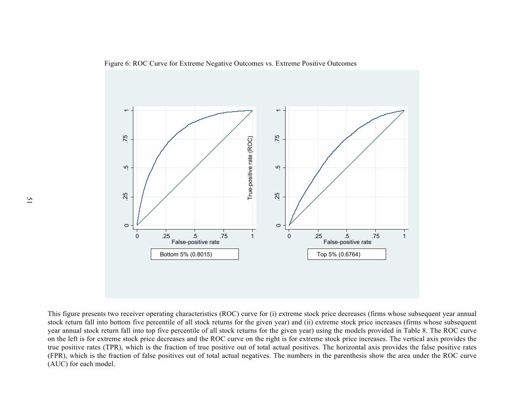
51

Figure 6: ROC Curve for Extreme Negative Outcomes vs. Extreme Positive Outcomes

This figure presents two receiver operating characteristics (ROC) curve for (i) extreme stock price decreases (firms whose subsequent year annual stock return fall into bottom five percentile of all stock returns for the given year) and (ii) extreme stock price increases (firms whose subsequent year annual stock return fall into top five percentile of all stock returns for the given year) using the models provided in Table 8. The ROC curve on the left is for extreme stock price decreases and the ROC curve on the right is for extreme stock price increases. The vertical axis provides the true positive rates (TPR), which is the fraction of true positive out of total actual positives. The horizontal axis provides the false positive rates (FPR), which is the fraction of false positives out of total actual negatives. The numbers in the parenthesis show the area under the ROC curve (AUC) for each model.

0.2

5.5

.75

1

True

-pos

itive

rate

(RO

C)

0 .25 .5 .75 1False-positive rate

Bottom 5% (0.8015)

0.2

5.5

.75

1

True

-pos

itive

rate

(RO

C)

0 .25 .5 .75 1False-positive rate

Top 5% (0.6764)

52

Figure 7: Daily Stock Returns around Insider’s Trades by Quintiles of Financial Distress

Panel A: Daily Stock Returns when Insiders Purchase

Panel B: Daily Stock Returns when Insiders Sell

This figure is based on a total of 713,611 announcements of trading by top executives (CEO, CFO, COO, President, and Chairman of board with corresponding role codes of “CEO”, “CFO”, “CO”, “P”, and “CB” on the Thomson Reuters database). 95,899 observations are for top executives’ purchases, transaction code “P”, and the remaining 617,712 observations are for top executives’ sales. The returns are the average daily returns for each reported day for each distress risk quintile. Firms are sorted into quintiles based on their financial distress at the end of the month before the disclosure of the top executives’ trades.

-0.004

-0.002

0

0.002

0.004

0.006

0.008

0.01

0.012

-2 -1 0 1 2

Low Distress Risk

2nd Quintile

3rd Quintile

4th Quintile

High Distress Risk

-0.003-0.0025-0.002

-0.0015-0.001

-0.00050

0.00050.001

0.00150.002

0.0025

-2 -1 0 1 2

Low Distress Risk

2nd Quintile

3rd Quintile

4th Quintile

High Distress Risk

53

Figure 8: Monthly Excess Returns

This figure shows the future monthly excess returns to the investment strategy that takes a long position in financially distressed firms in which insiders are net purchasers using the 4-factor model and value weighted portfolio formation. 200 out of 323 observations are positive.

-40.0%

-30.0%

-20.0%

-10.0%

0.0%

10.0%

20.0%

30.0%

40.0%

50.0%Fe

brua

ry-8

8Fe

brua

ry-8

9Fe

brua

ry-9

0Fe

brua

ry-9

1Fe

brua

ry-9

2Fe

brua

ry-9

3Fe

brua

ry-9

4Fe

brua

ry-9

5Fe

brua

ry-9

6Fe

brua

ry-9

7Fe

brua

ry-9

8Fe

brua

ry-9

9Fe

brua

ry-0

0Fe

brua

ry-0

1Fe

brua

ry-0

2Fe

brua

ry-0

3Fe

brua

ry-0

4Fe

brua

ry-0

5Fe

brua

ry-0

6Fe

brua

ry-0

7Fe

brua

ry-0

8Fe

brua

ry-0

9Fe

brua

ry-1

0Fe

brua

ry-1

1Fe

brua

ry-1

2Fe

brua

ry-1

3Fe

brua

ry-1

4

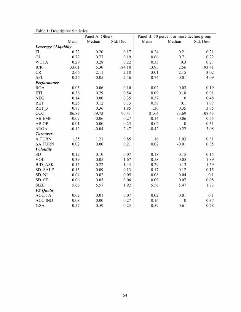
54

Table 1: Descriptive Statistics

Panel A: Others Panel B: 50 percent or more decline group

Mean Median Std. Dev. Mean Median Std. Dev.

Leverage / Liquidity

FL 0.22 0.20 0.17 0.24 0.21 0.21

OL 0.72 0.77 0.19 0.66 0.71 0.22 WCTA 0.29 0.28 0.22 0.33 0.3 0.27 ICR 33.01 5.30 184.18 13.95 2.56 193.41 CR 2.66 2.11 2.18 3.01 2.15 3.02 ΔFL 0.26 -0.05 2.46 0.74 -0.01 4.09 Performance

ROA 0.05 0.06 0.10 -0.02 0.03 0.19 ETL 0.36 0.29 0.54 0.09 0.18 0.91 NEG 0.14 0.00 0.35 0.37 0 0.48 RET 0.25 0.12 0.73 0.58 0.1 1.97 RET_3 0.77 0.36 1.85 1.36 0.35 3.75 CCC 86.83 79.73 90.41 81.64 73.69 108.43 AB.EMP -0.07 -0.06 0.27 -0.14 -0.06 0.55 AB.OB 0.01 0.00 0.25 0.02 0 0.31 ΔROA -0.12 -0.04 2.47 -0.42 -0.22 3.08 Turnover

A.TURN 1.35 1.21 0.85 1.16 1.03 0.81 ΔA.TURN 0.02 0.00 0.21 0.02 -0.01 0.35 Volatility

SD 0.12 0.10 0.07 0.18 0.15 0.15 VOL 0.39 -0.05 1.67 0.58 0.05 1.89 BID_ASK 0.15 -0.22 1.44 0.29 -0.13 1.59 SD_SALE 0.13 0.09 0.13 0.17 0.12 0.15 SD_NI 0.04 0.02 0.05 0.08 0.04 0.1 SD_CF 0.06 0.05 0.06 0.09 0.07 0.08 SIZE 5.66 5.57 1.92 5.56 5.47 1.73 FS Quality

ACC/TA 0.02 0.01 0.07 0.02 0.01 0.1 ACC.IND 0.08 0.00 0.27 0.16 0 0.37 %SA 0.57 0.59 0.23 0.59 0.61 0.28

55

Table 1: Descriptive Statistics - Continued

Panel A: Others Panel B: 50 percent or more decline group

Mean Median Std. Dev. Mean Median Std. Dev.

Torpedo

BtoM 1.39 0.58 5.89 0.82 0.39 4.01

E/P 0.12 0.06 0.58 0.02 0.03 0.36 ΔEQUITY -69.66 -1.40 376.99 -22.94 0.42 304.49 SHORT 19.23 0.83 41.64 26.38 0 53.8 SG 0.15 0.10 0.33 0.28 0.15 0.61 ΔE/P -0.05 0.01 2.48 -0.35 -0.17 3.22 DECLINE_SALES 0.22 0.00 0.42 0.25 0 0.43 CAPEX 0.07 0.05 0.06 0.07 0.04 0.07 This table includes the descriptive statistics for the main variables. Panel A report the descriptive statistics for the firms that do not experience a 50 percent or more stock price decline over the subsequent year. Panel B reports the descriptive statistics for firms that experience a 50 percent or more stock price decline. Correlations across explanatory variables have not been reported for the sake of brevity, they are available upon request.

56

Table 2: Logit Models

Accounting

Model Market Model Final Model Leverage / Liquidity FL 0.910***

0.811***

(9.15)

(8.56)

OL -0.372***

(-3.47)

WCTA 0.806***

0.499***

(6.42)

(4.30)

CR -0.035***

-0.017*

(-2.93)

(-1.72)

Performance ROA -1.205***

-0.627***

(-5.08)

(-3.30)

ETL -0.115***

-0.167***

(-3.04)

(-5.42)

NEG 0.924***

1.308***

(16.82)

(18.59)

RET_3

0.060*** 0.041***

(11.69) (7.08)

Turnover A.TURN -0.106***

-0.164***

(-3.46)

(-5.49)

ΔA.TURN -0.423***

-0.427***

(-4.99)

(-5.29)

Volatility SD

6.137*** 6.531***

(33.97) (23.74)

VOL

0.051*** 0.041***

(5.51) (4.67)

BID_ASK

-0.047***

(-4.14)

SD_SALE 0.925***

0.776***

(7.30)

(6.17)

SD_NI 4.391***

1.932***

(13.20)

(7.91)

SD_CF 1.591***

(5.61)

SIZE

-0.122*** -0.053*** (-12.90) (-4.54)

57

Table 2: Logit Models - Continued

Accounting

Model Market Model Final Model FS Quality

ACC/TA 1.551***

1.322***

(7.03)

(6.02)

ACC.IND 0.200***

0.165***

(3.91)

(3.26)

%SA 0.773***

0.745***

(7.91)

(7.92)

Torpedo BtoM

-0.017***

(-3.56)

E/P

-0.774***

(-10.25)

ΔEQUITY 0.000***

0.001***

(5.09)

(2.62)

SG 0.397***

0.346***

(8.03)

(7.23)

ΔE/P

-0.027***

(-5.29)

CAPEX 3.497***

3.050***

(11.57)

(10.24)

NEG_SD

-3.930***

(-11.39)

NEG_SD_NI -3.449***

(-6.74)

Constant -6.326*** -6.772*** -7.970***

(-4.96) (-4.54) (-5.30)

Observations 80,465 90,752 80,737 Pseudo R2 23% 22% 25% Time-Fixed Effects Yes Yes Yes Industry-Fixed Effects Yes Yes Yes

This table presents the logit model estimations for Equations 1, 2, and 3. The dependent variable is an indicator variable that takes the value of one if there is 50 percent or more stock price decline over the next year for a given firm and zero otherwise. Descriptions of explanatory variables are provided in Appendix A. The first column reports the coefficients for the accounting model, which incorporates only accounting variables. Column two reports the model for market variables and the final column reports the logistic regression coefficients for the combined model, which incorporates both accounting-based and market-based variables.

58

Table 3: Accuracy of the T-Score Panel A: Accounting Model Panel B: Market Model

#D %D Cum.%D Obs #D %D Cum.%D Obs

10 (High Prob) 1,438 28.53% 28.53% 7,966 10 (High Prob) 1,588 25.69% 25.69% 8,910

9 880 17.46% 45.99% 7,985 9 1,108 17.93% 43.62% 8,996 8 646 12.82% 58.81% 8,010 8 866 14.01% 57.63% 9,046 7 559 11.09% 69.90% 8,056 7 704 11.39% 69.02% 9,059 6 426 8.45% 78.35% 8,049 6 548 8.87% 77.88% 9,109 5 324 6.43% 84.78% 8,061 5 474 7.67% 85.55% 9,102 4 291 5.77% 90.56% 8,070 4 359 5.81% 91.36% 9,105 3 215 4.27% 94.82% 8,077 3 233 3.77% 95.13% 9,149 2 163 3.23% 98.06% 8,090 2 187 3.03% 98.16% 9,135

1 (Low Prob) 98 1.94% 100.00% 8,101 1 (Low Prob) 114 1.84% 100.00% 9,139

5,040 6,181

Panel C: Combined Model Panel D: Out-of-Sample Combined Model #D %D Cum.%D Obs #D %D Cum.%D Obs

10 (High Prob) 1,643 30.88% 30.88% 8,035 10 (High Prob) 1,588 25.69% 25.69% 8,910

9 984 18.49% 49.37% 8,057 9 1,108 17.93% 43.62% 8,996 8 725 13.63% 63.00% 8,076 8 866 14.01% 57.63% 9,046 7 570 10.71% 73.71% 8,064 7 704 11.39% 69.02% 9,059 6 460 8.64% 82.35% 8,074 6 548 8.87% 77.88% 9,109 5 316 5.94% 88.29% 8,067 5 474 7.67% 85.55% 9,102 4 239 4.49% 92.78% 8,082 4 359 5.81% 91.36% 9,105 3 185 3.48% 96.26% 8,089 3 233 3.77% 95.13% 9,149 2 128 2.41% 98.67% 8,091 2 187 3.03% 98.16% 9,135

1 (Low Prob) 71 1.33% 100.00% 8,102 1 (Low Prob) 114 1.84% 100.00% 9,139

5,321 6,181

59

Table 3: Accuracy of the T-Score - Ctd.

This table presents the actual observations of 50 percent or more stock price declines for the deciles of T-Score. I sort firms into deciles based on their T-Score each year. The highest decile contains the firms with highest T-Scores and the lowest decile incorporates firms with lowest T-Scores. #D is the number of firms with 50 percent or more stock price decline. %D represents the ratio of actual 50 percent or more stock price declines that is observed in each decile to the total number of 50 percent or more stock price declines. Cum.%D represents the cumulative percentage, and the final column represents the number of observations under each decile. Panel A of this table presents the accuracy results for the accounting-based model while Panel B reports the results for the market-based model. In Panel C, I report the accuracy results for the combined model for the in-sample T-Score and Panel D presents the results for the expanding-window out-of-sample T-Score.

60

Table 4: Properties of the Deciles of T-Score

T BtoM Size B C DD Z P ROA Ab.Emp Sell Recommendations

Underperform Recommendations

10 3.097 0.571 4.811 0.012 0.011 0.084 4.764 3.638 -6.90% -10.80% 2.50% 5.30% Trouble - 9 1.69 0.767 5.055 0.009 0.009 0.064 4.375 3.925 -0.60% -7.40% 2.20% 5.20%

8 1.231 0.85 5.165 0.006 0.008 0.054 4.33 4.32 2.60% -7.40% 2.10% 5.20% 7 0.946 0.965 5.341 0.004 0.007 0.045 4.5 4.624 4.30% -7.40% 1.70% 5.10% 6 0.754 0.94 5.473 0.002 0.007 0.037 4.705 4.804 5.20% -7.10% 2.50% 4.40% 5 0.619 1.006 5.674 0.002 0.006 0.032 4.682 4.862 5.80% -7.00% 1.90% 4.20% 4 0.515 1.104 5.864 0.002 0.005 0.03 4.721 4.884 6.30% -6.30% 2.70% 5.10% 3 0.425 1.257 6.1 0.001 0.005 0.031 4.878 4.904 6.90% -6.00% 2.10% 5.20%

Safe - 2 0.336 1.687 6.413 0.001 0.004 0.035 5.105 4.92 7.40% -6.30% 2.40% 6.00% 1 0.206 4.259 6.932 0.001 0.004 0.068 5.059 4.991 8.40% -6.70% 2.60% 6.60%

Troubled 2.005 0.730 5.010 0.009 0.010 0.043 4.486 3.961 -1.63% -11.59% 2.28% 5.23% Others 0.709 1.004 5.588 0.002 0.006 0.022 4.652 4.794 5.40% -6.45% 2.19% 4.70%

Safe 0.322 2.402 6.482 0.001 0.004 0.036 5.011 4.939 7.56% -5.01% 2.39% 5.96% Troubled - Safe 1.683* -1.672* -1.472* 0.008* 0.005* 0.008* -0.525* -0.977* -9.20%* -6.58%* -0.12% -0.73%

* p<0.01This table provides statistics about the deciles of the T-Score. I sort firms into deciles based on their T-Score every year. Highest decile contains the firms with highest T-Scores and the lowest decile incorporates firms with lowest T-Scores. T is the T-Score, BtoM is the book-to-market ratio, Size is the logarithm of the market capitalization of firms, DD is the distance-to-default measure, Z is Altman’s Z-Score, B is the distress risk model based on Beaver et al. (2012), P is Piotroski (2000) score, and C is the distress risk measure from Campbell et al. (2008). ROA is the one-year ahead Return on Asset; Ab.Emp is the one-year ahead abnormal change in employee, percentage change in the number of employees minus percentage change in total assets. Sell recommendations is the percentage of analysts’ sell recommendations to all analysts’ recommendations and similarly underperform recommendations is the percentage of analysts’ underperform recommendations to all recommendations. Troubled group consists of firms with Trouble Score deciles of 8 to 10, and Safe group consists of firms with Trouble Score deciles 1-3, and others are the firms with Trouble Score deciles between 4-7.

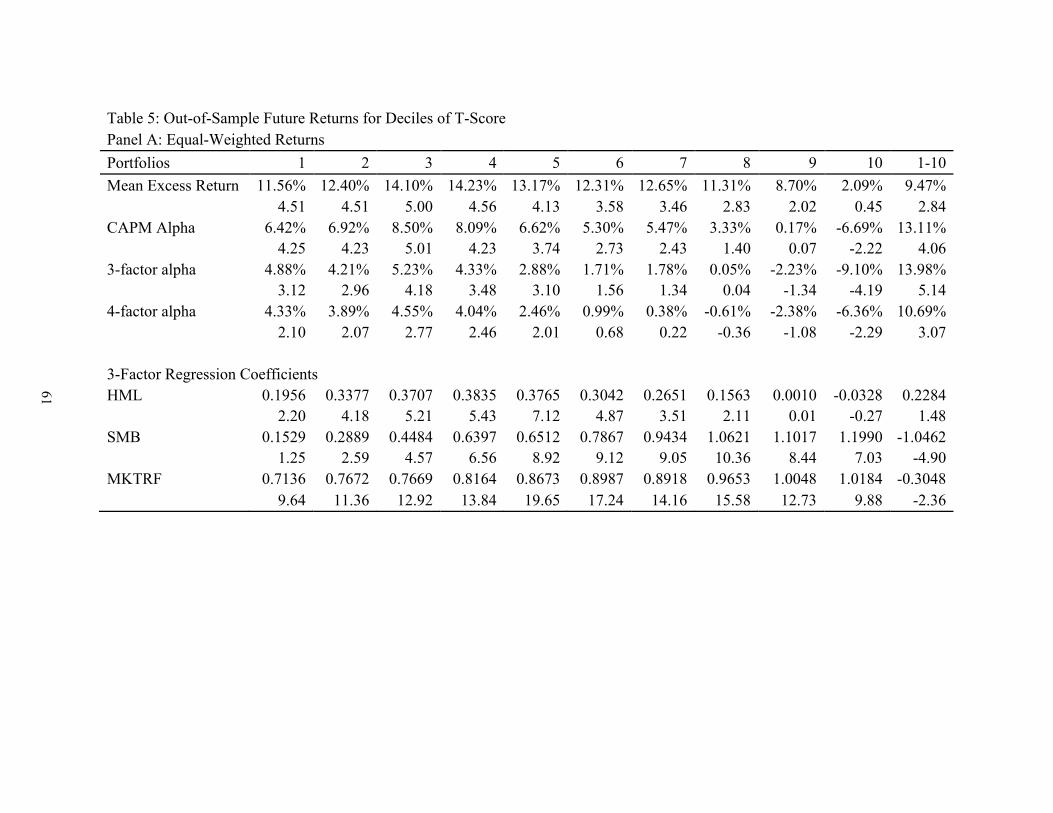
61

Table 5: Out-of-Sample Future Returns for Deciles of T-Score Panel A: Equal-Weighted Returns Portfolios 1 2 3 4 5 6 7 8 9 10 1-10 Mean Excess Return 11.56% 12.40% 14.10% 14.23% 13.17% 12.31% 12.65% 11.31% 8.70% 2.09% 9.47%

4.51 4.51 5.00 4.56 4.13 3.58 3.46 2.83 2.02 0.45 2.84 CAPM Alpha 6.42% 6.92% 8.50% 8.09% 6.62% 5.30% 5.47% 3.33% 0.17% -6.69% 13.11%

4.25 4.23 5.01 4.23 3.74 2.73 2.43 1.40 0.07 -2.22 4.06 3-factor alpha 4.88% 4.21% 5.23% 4.33% 2.88% 1.71% 1.78% 0.05% -2.23% -9.10% 13.98%

3.12 2.96 4.18 3.48 3.10 1.56 1.34 0.04 -1.34 -4.19 5.14 4-factor alpha 4.33% 3.89% 4.55% 4.04% 2.46% 0.99% 0.38% -0.61% -2.38% -6.36% 10.69%

2.10 2.07 2.77 2.46 2.01 0.68 0.22 -0.36 -1.08 -2.29 3.07

3-Factor Regression Coefficients HML 0.1956 0.3377 0.3707 0.3835 0.3765 0.3042 0.2651 0.1563 0.0010 -0.0328 0.2284

2.20 4.18 5.21 5.43 7.12 4.87 3.51 2.11 0.01 -0.27 1.48 SMB 0.1529 0.2889 0.4484 0.6397 0.6512 0.7867 0.9434 1.0621 1.1017 1.1990 -1.0462

1.25 2.59 4.57 6.56 8.92 9.12 9.05 10.36 8.44 7.03 -4.90 MKTRF 0.7136 0.7672 0.7669 0.8164 0.8673 0.8987 0.8918 0.9653 1.0048 1.0184 -0.3048

9.64 11.36 12.92 13.84 19.65 17.24 14.16 15.58 12.73 9.88 -2.36

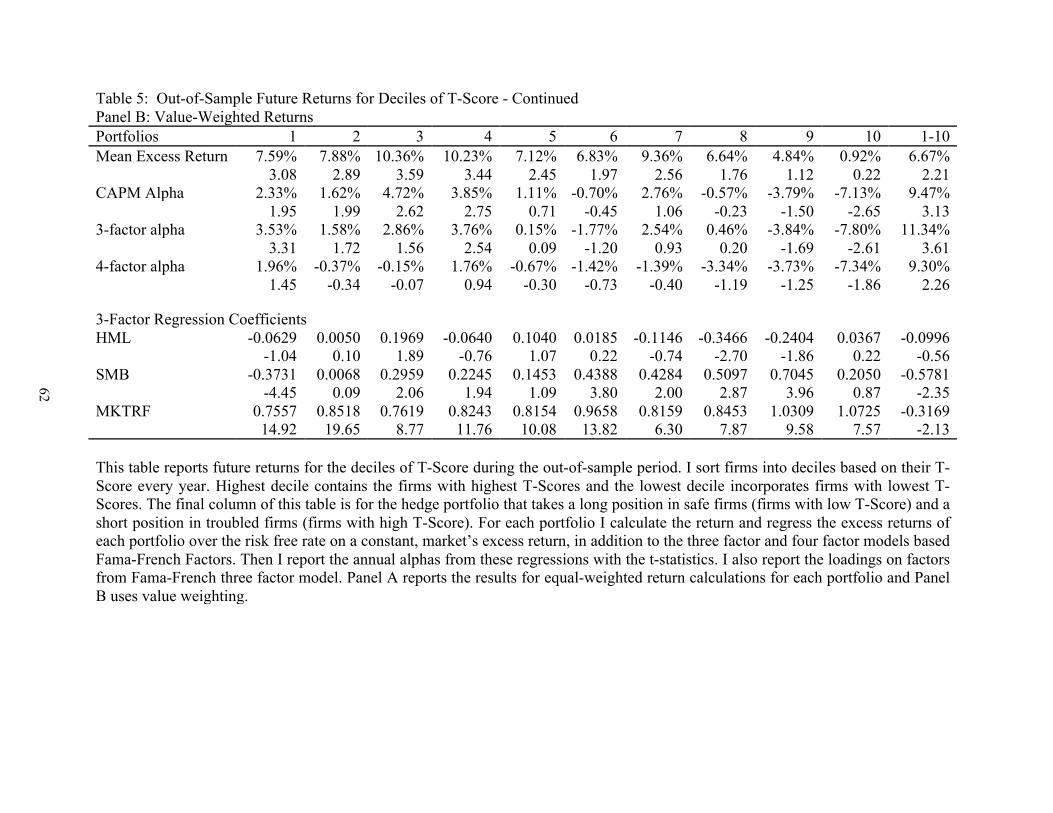
62

Table 5: Out-of-Sample Future Returns for Deciles of T-Score - Continued Panel B: Value-Weighted Returns Portfolios 1 2 3 4 5 6 7 8 9 10 1-10 Mean Excess Return 7.59% 7.88% 10.36% 10.23% 7.12% 6.83% 9.36% 6.64% 4.84% 0.92% 6.67%

3.08 2.89 3.59 3.44 2.45 1.97 2.56 1.76 1.12 0.22 2.21 CAPM Alpha 2.33% 1.62% 4.72% 3.85% 1.11% -0.70% 2.76% -0.57% -3.79% -7.13% 9.47%

1.95 1.99 2.62 2.75 0.71 -0.45 1.06 -0.23 -1.50 -2.65 3.13 3-factor alpha 3.53% 1.58% 2.86% 3.76% 0.15% -1.77% 2.54% 0.46% -3.84% -7.80% 11.34%

3.31 1.72 1.56 2.54 0.09 -1.20 0.93 0.20 -1.69 -2.61 3.61 4-factor alpha 1.96% -0.37% -0.15% 1.76% -0.67% -1.42% -1.39% -3.34% -3.73% -7.34% 9.30%

1.45 -0.34 -0.07 0.94 -0.30 -0.73 -0.40 -1.19 -1.25 -1.86 2.26

3-Factor Regression Coefficients HML -0.0629 0.0050 0.1969 -0.0640 0.1040 0.0185 -0.1146 -0.3466 -0.2404 0.0367 -0.0996

-1.04 0.10 1.89 -0.76 1.07 0.22 -0.74 -2.70 -1.86 0.22 -0.56 SMB -0.3731 0.0068 0.2959 0.2245 0.1453 0.4388 0.4284 0.5097 0.7045 0.2050 -0.5781

-4.45 0.09 2.06 1.94 1.09 3.80 2.00 2.87 3.96 0.87 -2.35 MKTRF 0.7557 0.8518 0.7619 0.8243 0.8154 0.9658 0.8159 0.8453 1.0309 1.0725 -0.3169

14.92 19.65 8.77 11.76 10.08 13.82 6.30 7.87 9.58 7.57 -2.13

This table reports future returns for the deciles of T-Score during the out-of-sample period. I sort firms into deciles based on their T-Score every year. Highest decile contains the firms with highest T-Scores and the lowest decile incorporates firms with lowest T-Scores. The final column of this table is for the hedge portfolio that takes a long position in safe firms (firms with low T-Score) and a short position in troubled firms (firms with high T-Score). For each portfolio I calculate the return and regress the excess returns of each portfolio over the risk free rate on a constant, market’s excess return, in addition to the three factor and four factor models based Fama-French Factors. Then I report the annual alphas from these regressions with the t-statistics. I also report the loadings on factors from Fama-French three factor model. Panel A reports the results for equal-weighted return calculations for each portfolio and Panel B uses value weighting.

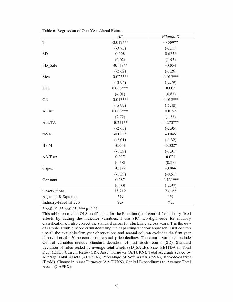
63

Table 6: Regression of One-Year Ahead Returns All Without D

T -0.017*** -0.009** (-3.73) (-2.11)

SD 0.008 0.625* (0.02) (1.97)

SD_Sale -0.119** -0.054 (-2.62) (-1.26)

Size -0.023*** -0.019*** (-2.94) (-2.79)

ETL 0.033*** 0.005 (4.01) (0.63)

CR -0.013*** -0.012*** (-5.99) (-5.48)

A.Turn 0.033*** 0.019* (2.72) (1.73)

Acc/TA -0.251** -0.270*** (-2.65) (-2.95)

%SA -0.083* -0.045 (-2.01) (-1.32)

BtoM -0.002 -0.002* (-1.59) (-1.91)

ΔA.Turn 0.017 0.024 (0.58) (0.88)

Capex -0.199 -0.066 (-1.39) (-0.51)

Constant 0.387 -0.131*** (0.00) (-2.97)

Observations 78,212 73,166 Adjusted R-Squared 2% 1% Industry-Fixed Effects Yes Yes * p<0.10, ** p<0.05, *** p<0.01This table reports the OLS coefficients for the Equation (4). I control for industry fixed effects by adding the indicator variables. I use SIC two-digit code for industry classifications. I also correct the standard errors for clustering across years. T is the out-of sample Trouble Score estimated using the expanding window approach. First column use all the available firm-year observations and second column excludes the firm-year observations for 50 percent or more stock price declines. The control variables include Control variables include Standard deviation of past stock returns (SD), Standard deviation of sales scaled by average total assets (SD_SALE), Size, EBITDA to Total Debt (ETL), Current Ratio (CR), Asset Turnover (A.TURN), Total Accruals scaled by Average Total Assets (ACC/TA), Percentage of Soft Assets (%SA), Book-to-Market (BtoM), Change in Asset Turnover (ΔA.TURN), Capital Expenditures to Average Total Assets (CAPEX).

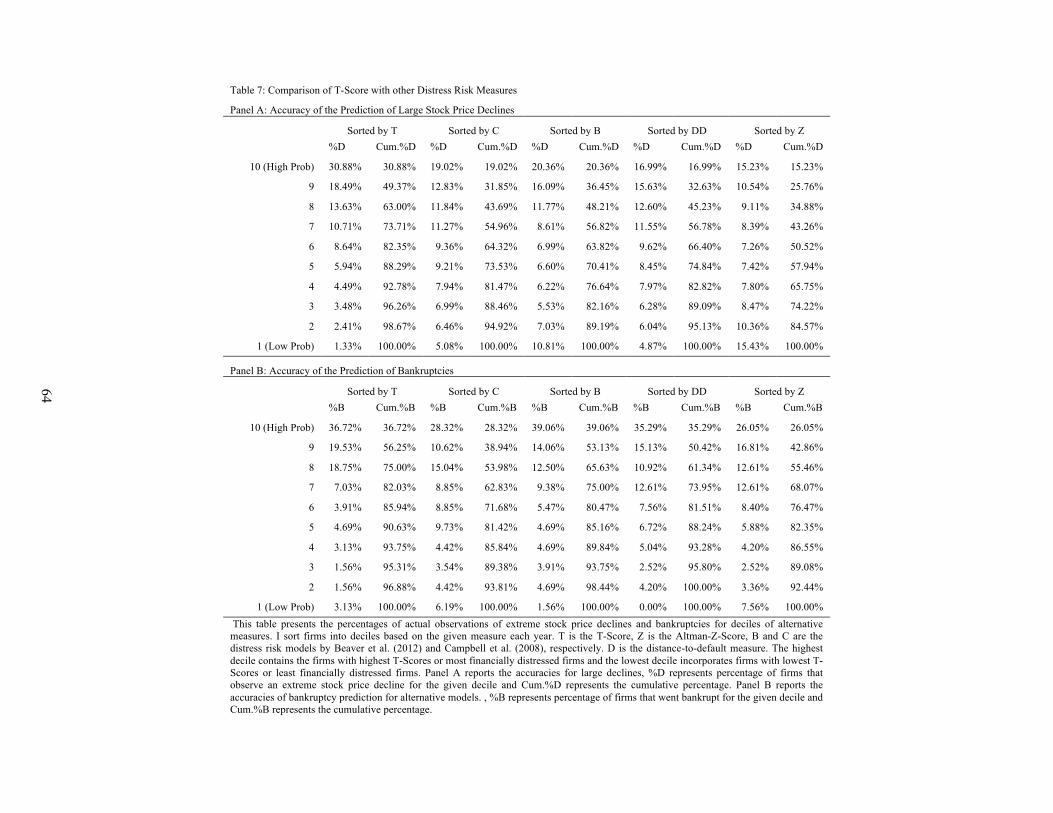
64

Table 7: Comparison of T-Score with other Distress Risk Measures

Panel A: Accuracy of the Prediction of Large Stock Price Declines

Sorted by T Sorted by C Sorted by B Sorted by DD Sorted by Z %D Cum.%D %D Cum.%D %D Cum.%D %D Cum.%D %D Cum.%D

10 (High Prob) 30.88% 30.88% 19.02% 19.02% 20.36% 20.36% 16.99% 16.99% 15.23% 15.23%

9 18.49% 49.37% 12.83% 31.85% 16.09% 36.45% 15.63% 32.63% 10.54% 25.76%

8 13.63% 63.00% 11.84% 43.69% 11.77% 48.21% 12.60% 45.23% 9.11% 34.88%

7 10.71% 73.71% 11.27% 54.96% 8.61% 56.82% 11.55% 56.78% 8.39% 43.26%

6 8.64% 82.35% 9.36% 64.32% 6.99% 63.82% 9.62% 66.40% 7.26% 50.52%

5 5.94% 88.29% 9.21% 73.53% 6.60% 70.41% 8.45% 74.84% 7.42% 57.94%

4 4.49% 92.78% 7.94% 81.47% 6.22% 76.64% 7.97% 82.82% 7.80% 65.75%

3 3.48% 96.26% 6.99% 88.46% 5.53% 82.16% 6.28% 89.09% 8.47% 74.22%

2 2.41% 98.67% 6.46% 94.92% 7.03% 89.19% 6.04% 95.13% 10.36% 84.57%

1 (Low Prob) 1.33% 100.00% 5.08% 100.00% 10.81% 100.00% 4.87% 100.00% 15.43% 100.00%

Panel B: Accuracy of the Prediction of Bankruptcies

Sorted by T Sorted by C Sorted by B Sorted by DD Sorted by Z %B Cum.%B %B Cum.%B %B Cum.%B %B Cum.%B %B Cum.%B

10 (High Prob) 36.72% 36.72% 28.32% 28.32% 39.06% 39.06% 35.29% 35.29% 26.05% 26.05%

9 19.53% 56.25% 10.62% 38.94% 14.06% 53.13% 15.13% 50.42% 16.81% 42.86%

8 18.75% 75.00% 15.04% 53.98% 12.50% 65.63% 10.92% 61.34% 12.61% 55.46%

7 7.03% 82.03% 8.85% 62.83% 9.38% 75.00% 12.61% 73.95% 12.61% 68.07%

6 3.91% 85.94% 8.85% 71.68% 5.47% 80.47% 7.56% 81.51% 8.40% 76.47%

5 4.69% 90.63% 9.73% 81.42% 4.69% 85.16% 6.72% 88.24% 5.88% 82.35%

4 3.13% 93.75% 4.42% 85.84% 4.69% 89.84% 5.04% 93.28% 4.20% 86.55%

3 1.56% 95.31% 3.54% 89.38% 3.91% 93.75% 2.52% 95.80% 2.52% 89.08%

2 1.56% 96.88% 4.42% 93.81% 4.69% 98.44% 4.20% 100.00% 3.36% 92.44%

1 (Low Prob) 3.13% 100.00% 6.19% 100.00% 1.56% 100.00% 0.00% 100.00% 7.56% 100.00% This table presents the percentages of actual observations of extreme stock price declines and bankruptcies for deciles of alternative measures. I sort firms into deciles based on the given measure each year. T is the T-Score, Z is the Altman-Z-Score, B and C are the distress risk models by Beaver et al. (2012) and Campbell et al. (2008), respectively. D is the distance-to-default measure. The highest decile contains the firms with highest T-Scores or most financially distressed firms and the lowest decile incorporates firms with lowest T-Scores or least financially distressed firms. Panel A reports the accuracies for large declines, %D represents percentage of firms that observe an extreme stock price decline for the given decile and Cum.%D represents the cumulative percentage. Panel B reports the accuracies of bankruptcy prediction for alternative models. , %B represents percentage of firms that went bankrupt for the given decile and Cum.%B represents the cumulative percentage.

65

Table 8: Predicting Extreme Negative Outcomes vs. Extreme Positive Outcomes Panel A: Logit Models

Bottom 5 Percentile

Top 5 Percentile

Bottom 5 Percentile

Top 5 Percentile

Leverage / Liquidity

FS Quality FL 0.860*** 0.665*** Acc/TA 1.821*** -0.939***

(7.43) (6.54) (7.07) (-4.35)

WCTA 0.731*** %SA 0.736*** -0.410***

(5.99) (6.48) (-4.62)

CR -0.079*** Torpedo

(-6.52) BtoM -0.019** -0.015***

Performance (-2.23) (-2.82) ROA 0.854*** E/P -0.581*** -0.127**

(4.45) (-4.40) (-2.19)

ETL -0.165*** ΔEquity 0.001***

(-5.07) (5.50)

Neg 1.259*** 0.362*** SG 0.371***

(14.79) (4.87) (6.62)

Ret_3 0.028*** Capex 2.646***

(4.18) (7.38)

Ab.Ob -0.171** 0.120** RD 2.269***

(-2.32) (2.16) (8.58)

Turnover Short 0.002*** 0.003*** A.Turn -0.216*** 0.101*** (3.31) (6.79)

(-5.34) (3.94)

ΔA.Turn -0.335*** 0.186***

(-3.53) (3.17) Neg_SD -2.908*** -1.478***

Volatility (-7.59) (-4.16) SD 4.858*** 1.812*** Constant -18.91 -1.372**

(15.24) (7.53) (-0.01) (-2.46)

Vol 0.036***

(3.14)

Bid_Ask 0.040***

(3.97)

SD_Sale 0.699***

(4.19)

SD_NI 2.093***

(6.79)

SD_CF 1.379*** Observations 72,241 94,681

(4.10) Pseudo R2 13.2% 4.4%

Size -0.118*** -0.275*** Time-Fixed Effects Yes Yes (-7.24) (-23.77) Industry-Fixed Effects Yes Yes

66

Table 8: Predicting Extreme Negative Outcomes vs. Extreme Positive Outcomes - Ctd. Panel B: Accuracy of the Models Panel B-1: Accuracy for Bottom 5 Percentile

Panel B-2: Accuracy for Top 5 Percentile

#B %B Cum.%B Obs #T %T Cum.%T Obs

10 1,001 39.67% 39.67% 7,204

10 924 20.82% 20.82% 9,445 9 496 19.66% 59.33% 7,226

9 712 16.04% 36.86% 9,471

8 307 12.17% 71.50% 7,223

8 669 15.07% 51.94% 9,467 7 237 9.39% 80.90% 7,225

7 534 12.03% 63.97% 9,467

6 156 6.18% 87.08% 7,232

6 481 10.84% 74.81% 9,477 5 119 4.72% 91.80% 7,217

5 345 7.77% 82.58% 9,455

4 88 3.49% 95.28% 7,222

4 310 6.99% 89.57% 9,465 3 59 2.34% 97.62% 7,226

3 235 5.30% 94.86% 9,469

2 43 1.70% 99.33% 7,223

2 148 3.33% 98.20% 9,469 1 17 0.67% 100.00% 7,243

1 80 1.80% 100.00% 9,490

2,523 4,438 * p<0.10, ** p<0.05, *** p<0.01 This table compares the ability of accounting information when combined with market variables to predict extreme negative outcomes to the ability of accounting information when combined with market variables to predict extreme positive outcomes. Panel A reports the logit models for both extreme negative outcomes and extreme positive outcomes. For the bottom 5 percentile group, the dependent variable is an indicator variable that takes the value of one if the annual stock return the annual stock return of a firm over the next year falls into bottom five percentile of all the stock returns for the same year and zero otherwise. Similarly, for the Top 5 percentile group, the dependent variable is an indicator variable that takes the value of one if the annual stock return the annual stock return of a firm over the next year falls into top five percentile of all the stock returns for the same year and zero otherwise. Panel B reports the accuracies for the two models presented in Panel A. Panel B-1 reports the accuracies for the Bottom 5 percentile model, I sort firms into deciles based on their predicted probability each year. The highest decile contains the firms with highest probability of extreme negative outcome and the lowest decile incorporates firms with lowest probabilities. #B is the number of firms whose one year ahead stock returns is in the bottom fifth percentile and #NB is the number of firms that are not. %B represents the ratio of actual extreme stock price decreases that is observed in each decile to the total number extreme stock price decreases and Cum.%B represents the cumulative percentage. Panel B-2 reports the accuracies for the Top 5 percentile model, I sort firms into deciles based on their predicted probability each year. The highest decile contains the firms with highest probability of extreme positive outcome and the lowest decile incorporates firms with lowest probabilities. #T is the number of firms whose one year ahead stock returns is in the top fifth percentile and #NT is the number of firms that are not. %T represents the ratio of actual extreme stock price increases that is observed in each decile to the total number extreme stock price increases and Cum.%T represents the cumulative percentage. the final column represents The number of observations under each decile.

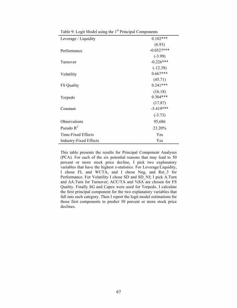
67

Table 9: Logit Model using the 1st Principal Components

Leverage / Liquidity 0.102***

(6.93)

Performance -0.0527***

(-3.99)

Turnover -0.226***

(-12.38)

Volatility 0.667***

(45.71)

FS Quality 0.241***

(16.18)

Torpedo 0.304***

(17.87)

Constant -5.419***

(-3.73)

Observations 95,686 Pseudo R2 23.20% Time-Fixed Effects Yes Industry-Fixed Effects Yes

This table presents the results for Principal Component Analyses (PCA). For each of the six potential reasons that may lead to 50 percent or more stock price decline, I pick two explanatory variables that have the highest z-statistics. For Leverage/Liquidity, I chose FL and WCTA, and I chose Neg, and Ret_3 for Performance. For Volatility I chose SD and SD_NI; I pick A.Turn and ΔA.Turn for Turnover; ACC/TA and %SA are chosen for FS Quality. Finally SG and Capex were used for Torpedo. I calculate the first principal component for the two explanatory variables that fall into each category. Then I report the logit model estimations for those first components to predict 50 percent or more stock price declines.

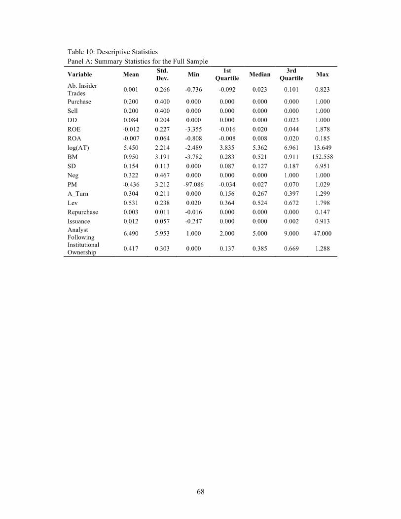
68

Table 10: Descriptive Statistics Panel A: Summary Statistics for the Full Sample

Variable Mean Std. Dev. Min 1st

Quartile Median 3rd Quartile Max

Ab. Insider Trades 0.001 0.266 -0.736 -0.092 0.023 0.101 0.823

Purchase 0.200 0.400 0.000 0.000 0.000 0.000 1.000 Sell 0.200 0.400 0.000 0.000 0.000 0.000 1.000 DD 0.084 0.204 0.000 0.000 0.000 0.023 1.000 ROE -0.012 0.227 -3.355 -0.016 0.020 0.044 1.878 ROA -0.007 0.064 -0.808 -0.008 0.008 0.020 0.185 log(AT) 5.450 2.214 -2.489 3.835 5.362 6.961 13.649 BM 0.950 3.191 -3.782 0.283 0.521 0.911 152.558 SD 0.154 0.113 0.000 0.087 0.127 0.187 6.951 Neg 0.322 0.467 0.000 0.000 0.000 1.000 1.000 PM -0.436 3.212 -97.086 -0.034 0.027 0.070 1.029 A_Turn 0.304 0.211 0.000 0.156 0.267 0.397 1.299 Lev 0.531 0.238 0.020 0.364 0.524 0.672 1.798 Repurchase 0.003 0.011 -0.016 0.000 0.000 0.000 0.147 Issuance 0.012 0.057 -0.247 0.000 0.000 0.002 0.913 Analyst Following 6.490 5.953 1.000 2.000 5.000 9.000 47.000

Institutional Ownership 0.417 0.303 0.000 0.137 0.385 0.669 1.288

69

Table 10: Summary Statistics – Continued Panel B: Summary Statistics by Abnormal Insider Trading

Sell Normal Purchase Purchase - Sell

Mean Median Mean Median Mean Median Mean

Ab. Insider Trades -0.383 -0.396 0.009 0.023 0.363 0.397 0.746**

DD 0.035 0.000 0.101 0.000 0.082 0.000 0.047** ROE 0.008 0.030 -0.020 0.016 -0.009 0.020 -0.017** ROA 0.003 0.013 -0.011 0.006 -0.005 0.008 -0.008** log(AT) 5.766 5.792 5.192 5.051 5.909 5.811 0.143** BM 0.517 0.393 1.099 0.569 0.937 0.552 0.42** SD 0.145 0.120 0.160 0.132 0.144 0.121 -0.001* Neg 0.229 0.000 0.358 0.000 0.308 0.000 0.079** PM -0.285 0.044 -0.522 0.021 -0.330 0.027 -0.045** A_Turn 0.316 0.280 0.300 0.263 0.303 0.267 -0.013** Lev 0.505 0.501 0.537 0.527 0.543 0.539 0.038** Repurchase 0.004 0.000 0.003 0.000 0.003 0.000 -0.001** Issuance 0.014 0.001 0.012 0.000 0.009 0.000 -0.005** Analyst Following 7.191 5.000 6.114 4.000 6.539 5.000 -0.652**

Institutional Ownership 0.519 0.542 0.367 0.301 0.451 0.444 -0.068**

70

Table 10: Summary Statistics – Continued

Panel C: Summary Statistics by Quintiles of Distance-to-Default

Low Distress Risk 2 3 4 High Distress

Risk High-Low

Ab. Insider Trades -0.068 -0.035 0.002 0.040 0.065 0.133**

Purchase 0.190 0.199 0.203 0.209 0.199 0.009**

Sell 0.309 0.258 0.203 0.142 0.089 -0.220**

DD 0.000 0.000 0.003 0.038 0.380 0.380**

ROE 0.032 0.015 -0.003 -0.026 -0.079 -0.111**

ROA 0.016 0.004 -0.005 -0.015 -0.035 -0.051**

log(AT) 6.259 5.882 5.433 4.982 4.693 -1.566**

BM 0.434 0.534 0.677 0.938 2.170 1.736**

SD 0.102 0.127 0.150 0.174 0.215 0.113**

Neg 0.121 0.196 0.286 0.404 0.607 0.486**

PM -0.137 -0.278 -0.441 -0.551 -0.772 -0.635**

A_Turn 0.320 0.306 0.302 0.302 0.291 -0.029**

Lev 0.407 0.479 0.525 0.576 0.670 0.263**

Repurchase 0.006 0.004 0.002 0.002 0.001 -0.005**

Issuance 0.011 0.014 0.014 0.012 0.009 -0.002**

Analyst Following 8.136 6.840 5.926 5.217 4.641 -3.495**

Institutional Ownership 0.539 0.497 0.434 0.344 0.240 -0.299**

* p<0.05, ** p<0.01 The summary statistics presented here are from a sample of 352,327 firm-quarter observations. First column in Panel B reports the mean values and the second column reports the median values. The final column in Panel B shows the results of the mean comparison test for insider purchasers and sellers. Panel C reports the mean statistics for variables across distress risk quintiles, and the final column runs a mean comparison test between most financially distressed firms and the least financially distressed firms. Ab. Insider Trades is the level of abnormal insider trading by top executives’ estimated as the residuals from Equation (9). I rank firms based on their level of abnormal insider trading into quintiles every quarter, the highest (the lowest) quintile captures the firms in which top executives purchased (sold) abnormally high number of shares. I use a rank quintile transformation, where the quarterly ranks are scaled to lie between 0.2 (lowest rank) and 1 (highest rank). Purchase (Sell) is an indicator variable that takes the value of one when the quintile of Ab. Insider Trades is one (zero), which classifies firm-quarter observations as insider’ being abnormal purchasers (abnormal sellers). ROE is calculated as the net income before extraordinary items (ibq) scaled by the average book value of equity (seqq+txditcq-pstkq); ROA is calculated as the net income before extraordinary items (ibq) scaled by the average total assets (atq); log(AT) is the logarithm of the total assets (atq). BM is calculated as the book value of equity book value of equity (seqq+txditcq-pstkq) scaled by the market value of equity (shrout*prc from CRSP). SD is measured as the standard deviation of the last 12 monthly stock returns. Neg is an indicator variable for loss quarters. PM is calculated as the net income before extraordinary items (ibq) scaled by the sales (saleq); A_Turn is calculated as the sales (saleq) scaled by the average book value of total assets (atq); Lev is calculated as the total liabilities (ltq) scaled by the total assets (atq). Repurchase is measured as the purchase of common and preferred stock (prstkcy) scaled by average total assets, and Issuance is measured as the sale of common stock and preferred stock (sstky) scaled by average total assets. Analyst Following is the number of analyst following gathered from IBES and Institutional Ownership is the level of institutional ownership gathered from Thomson Reuters Institutional Holdings (13f) database, measured as the number of shares held by institutional investors scaled by the number of shares outstanding.

71

Table 11: Top Executives’ Trades, Distress Risk, and Future Fundamental Firm Performance

ROEit+1 ROAit+1 PMit+1 A_Turnit+1 Levit+1 rank(DDit) -0.1185*** -0.0394*** -0.2459*** -0.0121*** 0.0289***

(-13.40) (-13.07) (-5.18) (-7.88) (14.64) rank(Ab.Insider Tradesit) -0.0132*** -0.0083*** -0.0641*** -0.0015 0.0052***

(-4.26) (-8.77) (-2.77) (-1.63) (5.23) rank(DDit)*rank(Ab.Insider Tradesit) 0.0225*** 0.0105*** 0.0914* 0.0033** -0.0051***

(3.22) (5.79) (1.94) (2.41) (-2.69) log(ATit) 0.0117*** 0.0077*** 0.0470*** -0.0027*** 0.0013***

(16.56) (24.87) (7.08) (-14.33) (5.22) BMit -0.0004 -0.0000 0.0017** 0.0001 -0.0002***

(-1.26) (-0.03) (2.05) (1.14) (-4.08) SGit -0.0043* -0.0043*** -0.5041*** -0.0425*** -0.0105***

(-1.93) (-6.59) (-11.74) (-19.28) (-12.50) PMit 0.0057*** 0.0049*** 0.7399*** 0.0001** -0.0006***

(9.08) (14.12) (26.78) (1.98) (-5.05) A_Turnit 0.0972*** 0.0587*** 0.6288*** 0.9101*** -0.0072***

(19.70) (22.99) (8.90) (188.07) (-4.50) Levit 0.0360*** -0.0219*** 0.2255*** 0.0242*** 0.9536***

(4.47) (-9.50) (4.87) (15.75) (362.76) Intercept -0.0614 -0.0128*** -0.4639*** 0.0335 -0.0027

(-0.00) (-3.30) (-3.59) (0.00) (-0.00) Industry F.E. Yes Yes Yes Yes Yes Quarter F. E. Yes Yes Yes Yes Yes Observations 352,327 352,317 351,644 352,172 352,274 Adjusted R2 6% 26% 57% 88% 91%

t statistics in parentheses * p<0.10, ** p<0.05, *** p<0.01 This table reports the OLS coefficients for Equation (11). The dependent variable in the regression is given in the top line. ROE is calculated as the net income before extraordinary items (ibq) scaled by the average book value of equity (seqq+txditcq-pstkq); ROA is calculated as the net income before extraordinary items (ibq) scaled by the average total assets (atq); PM is calculated as the net income before extraordinary items (ibq) scaled by the sales (saleq); A_Turn is calculated as the sales (saleq) scaled by the average book value of total assets (atq); Lev is calculated as the total liabilities (ltq) scaled by the total assets (atq).

72

Table 11: Top Executives’ Trades, Distress Risk, and Future Fundamental Firm Performance – Continued BM is calculated as the book value of equity book value of equity (seqq+txditcq-pstkq) scaled by the market value of equity (shrout*prc from CRSP). SG is the sales growth calculated by the percentage growth in sales (saleq) over the previous quarter. Distance-to-Default (DD) is the distress risk measure based on Black and Scholes (1973) and Merton (1974) estimated using the SAS procedure provided by Hillegeist et al. (2004). I use quintile rank transformations for distance-to-default. Specifically, firms are ranked quarterly and assigned to quintiles based on DD, where the quarterly ranks are scaled to lie between 0.2 (lowest rank) and 1 (highest rank). Ab. Insider Trades is the level of abnormal insider trading by top executives’ estimated as the residuals from Equation (9). I use quintile rank transformations for abnormal insider trading similar to the DD. All the models control for Industry Fixed Effects and the standard errors are corrected for clustering around time.

73

Table 12: Logit Models for Performance Related Delistings (1) (2) (3) DDit 3.277***

(39.25) Ab. Insider Tradesit -0.139**

(-2.02)

rank(DDit)

5.034*** 4.953***

(25.23) (24.89)

rank(Ab.Insider Tradesit) -0.379***

(-6.06)

Purchaseit

-0.529***

(-9.87)

Sellit

-0.263***

(-4.59)

log(ATit) -0.377*** -0.381*** -0.386***

(-17.26) (-16.38) (-16.36)

BMit -0.000 0.015*** 0.014***

(-0.01) (3.24) (3.02)

SDit 0.504*** 0.600*** 0.602***

(3.92) (5.14) (5.06)

ΔPMit 1.239*** 1.284*** 1.280***

(21.67) (24.28) (24.09)

Intercept -4.181*** -6.863*** -6.878***

(-17.09) (-20.43) (-20.29)

Industry F.E. Yes Yes Yes Quarter F.E. Yes Yes Yes Observations 351,171 351,171 351,171 Pseudo R2 26% 25% 25% z statistics in parentheses * p<0.10, ** p<0.05, *** p<0.01 This table reports the logit model estimation of the coefficients for Equation (12). The dependent variable takes the value of one value of one if a firm experiences a performance related delisting (CRSP delisting codes 400 and codes between 550 and 585) during the following quarter. All the explanatory variables are defined in Table 10 and 2.

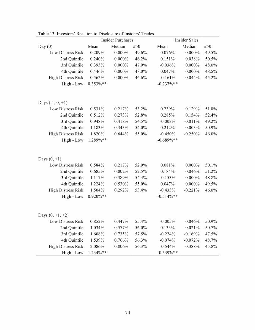
74

Table 13: Investors’ Reaction to Disclosure of Insiders’ Trades Insider Purchases Insider Sales

Day (0) Mean Median #>0

Mean Median #>0 Low Distress Risk 0.209% 0.000% 49.6%

0.076% 0.000% 49.5%

2nd Quintile 0.240% 0.000% 46.2%

0.151% 0.038% 50.5% 3rd Quintile 0.393% 0.000% 47.9%

-0.036% 0.000% 48.0%

4th Quintile 0.446% 0.000% 48.0%

0.047% 0.000% 48.5% High Distress Risk 0.562% 0.000% 46.6%

-0.161% -0.044% 45.2%

High - Low 0.353%**

-0.237%**

Days (-1, 0, +1)

Low Distress Risk 0.531% 0.217% 53.2%

0.239% 0.129% 51.8% 2nd Quintile 0.512% 0.273% 52.8%

0.285% 0.154% 52.4%

3rd Quintile 0.948% 0.418% 54.5%

-0.003% -0.011% 49.2% 4th Quintile 1.183% 0.343% 54.0%

0.212% 0.003% 50.9%

High Distress Risk 1.820% 0.644% 55.0%

-0.450% -0.250% 46.0% High - Low 1.289%**

-0.689%**

Days (0, +1)

Low Distress Risk 0.584% 0.217% 52.9%

0.081% 0.000% 50.1% 2nd Quintile 0.685% 0.002% 52.5%

0.184% 0.046% 51.2%

3rd Quintile 1.117% 0.389% 54.4%

-0.153% 0.000% 48.8% 4th Quintile 1.224% 0.530% 55.0%

0.047% 0.000% 49.5%

High Distress Risk 1.504% 0.292% 53.4%

-0.433% -0.221% 46.0% High - Low 0.920%**

-0.514%**

Days (0, +1, +2)

Low Distress Risk 0.852% 0.447% 55.4%

-0.005% 0.046% 50.9% 2nd Quintile 1.034% 0.577% 56.0%

0.133% 0.021% 50.7%

3rd Quintile 1.608% 0.735% 57.5%

-0.224% -0.169% 47.5% 4th Quintile 1.539% 0.766% 56.3%

-0.074% -0.072% 48.7%

High Distress Risk 2.086% 0.806% 56.3% -0.544% -0.388% 45.8% High - Low 1.234%**

-0.539%**

75

Table 13: Investors’ Reaction to Disclosure of Insiders’ Trades – Continued * p<0.05, ** p<0.01 This table is based on a total of 713,611 announcements of trading by top executives (CEO, CFO, COO, President, and Chairman of board with corresponding role codes of “CEO”, “CFO”, “CO”, “P”, and “CB” on the Thomson Reuters database). 95,899 observations are for top executives’ purchases, transaction code “P”, and the remaining 617,712 observations are for top executives’ sales. The returns are the average daily returns for each reported day for each distress risk quintile. Firms are sorted into quintiles based on their financial distress at the end of the month before the disclosure of the top executives’ trades. 8,354; 9,191; 14,907; 24,853; and 38,594 observations of top executives’ purchases fall into the first, second, third, fourth, and fifth quintile of financial distress respectively. 177,053, 128,415, 154,374, 95,509, 62,361 observations of top executives’ sales fall into the first, second, third, fourth, and fifth quintile of financial distress respectively. The non-uniform distribution of observations across distress risk quintiles is normal, because of possible multiple observations of same firm a given month. Day(0) represents the returns on the day when the insiders’ trades are disclosed to SEC. Days (-1, 0, +1) represents the returns including the previous day, announcement day, and the day after the disclosure of the insiders’ trades. Days (0, +1) is the cumulative return for the two-day period including the announcement day of the top executives’ trades and the day after. Days (0, +1, +2) is the three-day cumulative return including the announcement day return, and two-days after the announcement.

76

Table 14: Investors’ Reaction to Disclosure of Insiders’ Trades Across Subsamples

Panel A: Insider Purchases

Panel B: Insider Sales

Big Small Dif.

Big Small Dif.

Low Distress Risk 0.46% 1.27% 0.81%**

-0.03% 0.19% 0.22%**

High Distress Risk 1.93% 2.35% 0.42%**

-0.87% -0.25% 0.63%**

Dif. 1.47%** 1.08%** -0.84%** -0.44%**

Low High Dif.

Low High Dif.

Bid-Ask Bid-Ask Bid-Ask Bid-Ask Low Distress

Risk 0.62% 1.18% 0.56%**

0.03% -0.02% -0.05%*

High Distress Risk 1.36% 2.67% 1.31%**

-0.27% -0.58% -0.31%**

Dif. 0.74%** 1.49%** -0.30%** -0.56%**

Low Volume

High Volume Dif.

Low Volume

High Volume Dif.

Low Distress Risk 0.61% 1.54% 0.93%**

-0.03% 0.03% 0.05%*

High Distress Risk 1.69% 3.31% 1.63%**

-0.02% -0.80% -0.78%**

Dif. 1.08%** 1.77%** 0.00% -0.83%**

Low Volatility

High Volatility Dif.

Low Volatility

High Volatility Dif.

Low Distress Risk 0.84% 0.95% 0.11%

-0.08% 0.12% 0.20%**

High Distress Risk 1.48% 2.84% 1.36%**

0.10% -0.65% -0.76%**

Dif. 0.64%** 1.88%** 0.18%** -0.77%**

Low #Analyst

High #Analyst Dif.

Low #Analyst

High #Analyst Dif.

Low Distress Risk 0.59% 1.64% 1.05%**

0.10% -0.01% -0.11%**

High Distress Risk 2.40% 4.17% 1.77%**

-0.34% -0.54% -0.20%**

Dif. 1.81%** 2.52%** -0.44%** -0.53%**

Low %Ins. Owners

High %Ins. Owners Dif.

Low %Ins. Owners

High %Ins. Owners Dif.

Low Distress Risk 0.65% 1.61% 0.96%**

-0.10% 0.10% 0.20%**

High Distress Risk 2.10% 3.15% 1.05%**

-0.26% -0.52% -0.25%**

Dif. 1.45%** 1.54%** -0.16%** -0.62%**

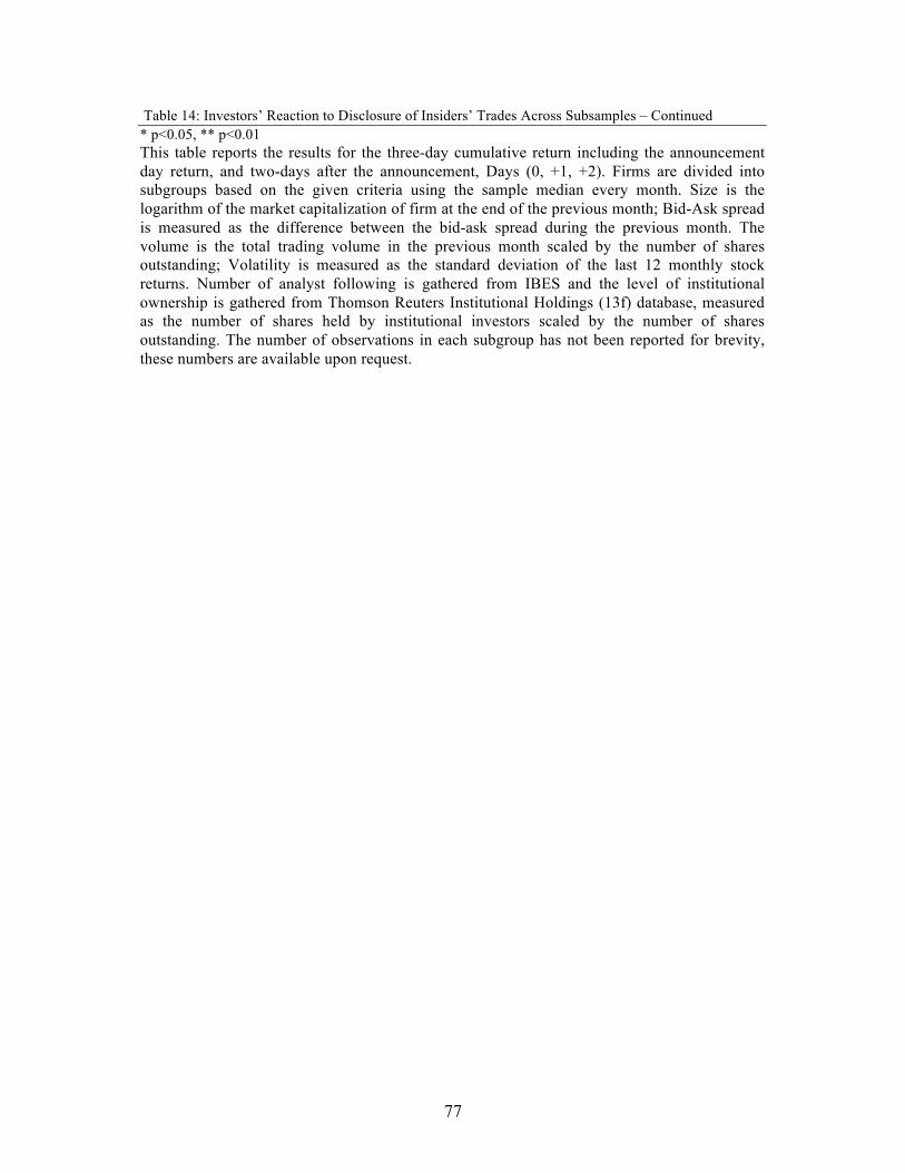
77

Table 14: Investors’ Reaction to Disclosure of Insiders’ Trades Across Subsamples – Continued * p<0.05, ** p<0.01 This table reports the results for the three-day cumulative return including the announcement day return, and two-days after the announcement, Days (0, +1, +2). Firms are divided into subgroups based on the given criteria using the sample median every month. Size is the logarithm of the market capitalization of firm at the end of the previous month; Bid-Ask spread is measured as the difference between the bid-ask spread during the previous month. The volume is the total trading volume in the previous month scaled by the number of shares outstanding; Volatility is measured as the standard deviation of the last 12 monthly stock returns. Number of analyst following is gathered from IBES and the level of institutional ownership is gathered from Thomson Reuters Institutional Holdings (13f) database, measured as the number of shares held by institutional investors scaled by the number of shares outstanding. The number of observations in each subgroup has not been reported for brevity, these numbers are available upon request.

78

Table 15: Future Excess Returns following Insiders’ Trades across Distress Risk Quintiles Panel A: Sell Q_DD 1 2 3 4 5 Mean Excess Return

%0.70*** %0.65* %0.75* %0.24 %0.49 (2.66) (1.91) (1.76) (0.45) (0.69)

CAPM Alpha %0.11 %-0.08 %-0.19 %-0.80** %-0.67

(0.70) (-0.40) (-0.77) (-2.11) (-1.18)

3-factor alpha %0.21 %-0.01 %-0.17 %-0.80** %-0.74

(1.51) (-0.04) (-0.70) (-2.15) (-1.31)

4-factor alpha %0.02 %0.00 %-0.09 %-0.42 %0.08 (0.17) (-0.02) (-0.37) (-1.16) (0.16)

Panel B: Purchases Q_DD 1 2 3 4 5 Mean Excess Return

%0.54 %0.92** %1.31*** %1.50*** %2.37*** (1.38) (2.35) (3.39) (3.12) (4.08)

CAPM Alpha %0.01 %0.32 %0.60** %0.64* %1.54***

(0.03) (0.98) (2.07) (1.77) (3.07)

3-factor alpha %0.09 %0.31 %0.50* %0.56 %1.43***

(0.26) (0.93) (1.74) (1.62) (2.91)

4-factor alpha %0.07 %0.41 %0.75*** %0.89*** %2.08*** (0.20) (1.23) (2.66) (2.62) (4.47) * p<0.10, ** p<0.05, *** p<0.01

This table reports to future returns for the quintiles of Distance-to-Default (DD). I sort firms into quintiles based on their DD every month. Highest quintile contains the most financially distressed firms and the lowest decile incorporates firms with lowest distress risk. For each portfolio I calculate the value-weighted return and regress the excess returns of each portfolio over the risk free rate on a constant, market’s excess return (MKTRF), in addition to the three factor and four factor models based Fama-French Factors. Then I report the annual alphas from these regressions with the t-statistics.

79

Table 16: Four-Factor Excess Returns Across Subsamples for Financially Distressed Firms in Which Insiders Were Net Purchasers

Big Small 1.94%*** 2.56%***

(2.69) (6.06)

Low Bid-Ask High Bid-Ask

2.52%*** 1.82%*** (3.85) (3.49)

Low Volume High Volume

3.00%*** 2.38%*** (5.63) (3.65)

Low Volatility High Volatility

3.06%*** 2.59%*** (4.75) (5.15)

Low #Analyst High #Analyst

2.26%*** 0.28% (3.00) (0.38)

Low %Ins. Owners High %Ins. Owners

2.67%*** 1.64%*** (4.67) (2.48)

This table reports the monthly value-weighted four-factor excess returns to the financially distressed firms in which top executives were net purchasers in the previous month. Firms are divided into subgroups based on the given criteria using the sample median every month. Size is the logarithm of the market capitalization of firm at the end of the previous month; Bid-Ask spread is measured as the difference between the bid-ask spread during the previous month. The volume is the total trading volume in the previous month scaled by the number of shares outstanding; Volatility is measured as the standard deviation of the last 12 monthly stock returns. Number of analyst following is gathered from IBES and the level of institutional ownership is gathered from Thomson Reuters Institutional Holdings (13f) database, measured as the number of shares held by institutional investors.