Essays on Economic Modeling of Climate Change - DiVA Portal
151
Transcript of Essays on Economic Modeling of Climate Change - DiVA Portal

Essays on Economic Modeling ofClimate Change
Gustav Engström

ii
c© Gustav Engström, Stockholm, 2012
ISBN 978-91-7447-541-8.ISSN 1404-3491
Cover picture: Gustav's desk.c© Gustav Engström
Printed in Sweden by PrintCenter US-AB, Stockhom 2012Distributor: Department of Economics, Stockholm University

iii
Doctoral DissertationDepartment of EconomicsStockholm University
Abstract
This thesis consists of three self-contained essays dealing with dierent aspects of theeconomics of climate change.
Structural change in a two-sector model of the climate and the economy
This paper introduces issues concerning substitution possibilities among goods into atwo-sector macroeconomic growth model where emissions from fossil fuels give rise toa climate externality. Substitution possibilities are modeled using a constant elasticityof substitution (CES) production function where the intermediate inputs dier only intheir technologies and the way they are aected by the climate externality. By solvingthe social planners problem and characterizing the competitive equilibrium I am able toderive a simple formula for optimal taxes and resource allocation over time. The impactof dierent assumptions regarding the elasticity of substitution on taxes turns out tobe a simple function of the size or relative magnitude of the distribution parameter ofthe CES function, technology and the impact of the climate externality. In particular,it is shown that a higher (lower) elasticity of substitution will result in a higher (lower)optimal unit tax rate if and only if the distribution parameter of the most produc-tive sector, multiplied by its total factor productivity and climate damage function, issmaller (larger) than the corresponding term of the other sector. I also present some nu-merical simulations for a calibrated model based on the U.S. and Indian economy. Theresults show that the assumptions regarding substitution possibilities plays a much big-ger role for optimal fossil fuel consumption in the agriculturally intense Indian economy.
Energy Balance Climate Models and General Equilibrium Optimal
Mitigation Policies
In a general equilibrium model of the world economy, we develop a one-dimensionalenergy balance climate model with heat diusion and anthropogenic forcing across lati-tudes driven by global fossil fuel use. This introduces an endogenous latitude dependenttemperature function, driving spatial characteristics, in terms of location dependentdamages resulting from local temperature anomalies into the standard climate-economyframework. We solve the social planner's problem and characterize the competitiveequilibrium for three separate cases dierentiated by the degree of market integrationand assumptions regarding costs of transfers. We dene optimal taxes on fossil fuel useand how they can implement the planning solution. Our results suggest that if the im-plementation of international transfers across latitudes are not possible or costly, then
iv
optimal taxes are in general spatially non-homogeneous and may be lower at poorerlatitudes. The degree of spatial dierentiation of optimal taxes depend on heat trans-portation. By employing the properties of the spatial model, we show by numericalsimulations how the impact of thermal transport across latitudes on welfare can bestudied.
Energy Balance Climate Models, Damage Reservoirs and the Time Prole
of Climate Change Policy
We explore optimal mitigation policies through the lens of a latitude dependent energybalance climate model, featuring an endogenously driven polar ice cap. We associatethe movement of the polar ice cap with the idea of a damage reservoir being a nitesource of climate related damages aecting the economy only to the extent that therestill exists some ice left to melt. We capture this idea by coupling this model with asimple economic growth model. We show that the endogenous ice line characteristicof our energy balance climate model induces a nonlinearity in the model. This non-linearity when combined with two sources of damages - the conventional damages dueto temperature increase and the reservoir damages - generates multiple steady statesand Skiba points. When introducing these concepts into the fairly mainstream DICEmodel of William Nordhaus it is shown that the policy ramp implied by the model callsfor high mitigation now. The simulation results further suggests that the policy rampcould be u-shaped instead of a the monotonically increasing gradualistic policy ramp.
Assessing Sustainable Development in a DICE World
This paper investigates a method for assessing sustainable development under climatechange in the Dynamic Integrated model of Climate and the Economy (DICE-2007model). The analysis shows that the results, with respect to sustainability are highlysensitive to the calibration of the social welfare function. When revising the social wel-fare parameters of the DICE-2007 model to the alternative parametrization approach,used in the DICE-(1994,1999) model, it is only the former that upholds a sustain-able productive base. This nding implies that when recalibrating the social welfarefunction, to match historical rates of return on capital, this can result in inconsistentprojections of future social welfare. The robustness of these results are investigated byimposing uncertainty, regarding key parameter estimates. This shows that the socialwelfare parameters along with total factor productivity growth are much more impor-tant as determinants of productive base sustainability than climatic parameters suchas the damage or temperature sensitivity coecients.

v
Acknowledgments
First and foremost, I would like to express my deepest gratitude to the people at theBeijer Institute of Ecological Economics, in particular, Carl Folke and Anne-SophieCrépin (co-supervisor). Without their belief in me this thesis would never have beenwritten. Anne-Sophie has provided me with great support and guidance and served asboth a professional and private mentor in all types of matters.
The Beijer Institute is a fantastic environment to do research in, with an opennessand warmth unheard of. I will never forget my rst days at the oce. Prior to myarrival I had only had a chance to interact with a Anne-Sophie, Therese and Ingela,mainly through email correspondence concerning the course on Ecological Economics,which I was attending at a distance. On the morning, of my rst day Christina andAgneta kindly showed me around the building and where I would be working. Afterthat it didn't take long before my rst, what I would like to call, "Beijer moment",occured. This happened when Åsa stumbled into the oce. She was wearing a blacktank top, a pair of "don't mess with me" type leather boots, hair colored in dierentshades of blonde/blue and with a piece of saran plastic wrapping around her rightshoulder. She was very friendly and talking at about a hundred miles an hour when Inally after 10-20 minutes or so, got around to asking here about the plastic aroundher shoulder. She responded that she had just been at the tatoo parlour and recievedthis awesome tatoo featuring a "morbid angle" that I would get to see in a couple days,when the plastic could be removed. About this time Calle "The Director" came by andpresented himself. He was a well dressed guy, wearing nice and tidy clothes, tting fora director of an international research institute. He was super friendly and insured meseveral times that he was extremely pleased that I had joined the work force. Åsa, fullof energy, was quick to let him know that she had just acquired this amazing piece ofink on her shoulder and insured him that tattoo guy was one of the best in Stockholmand if he ever wanted to get a tattoo she would gladly give him his number, and metoo for that matter. The rest of the day continued somewhat in this manner and Ican't remember getting much work done. In sum, my rst day at Beijer was a heartwarming experience with a lot of laughter and I quickly got the feeling that this placedid not draw a sharp line between work and private life and that there was an overallacceptance for the strange and unconventional. This is something that I am now gladand proud to be apart of and which I can also still conrm to be true.
Concerning research, my rst month at Beijer also became an extraordinary experi-ence. Calle invited me to participate in the annual meeting on the island of Askö whichwas held in conjunction with the Beijer board meeting. The Askö meeting has becomeknown as an great example of a successful transdiciplinary research, where top scholarsfrom around the world meet once a year to discuss a pressing topic related to globalenvironmental problems. The researchers invited vary, but the year I participated, theguest list included, Kenneth Arrow, a Nobel prize winner in economics, which had madeseveral important contributions to a variety of dierent elds including almost all ofthe chapters in the horrible (but also excellent) book by Mas-Colell, Whinston and

vi
Green which strikes fear in the eyes of most graduate students during their rst com-pulsory courses in Micro-economics. The amazing thing about this meeting was thatapart from getting to listen in on the fantastic discussions taking place in the meetingrooms, the trip also resulted in me becoming a co-author of the article "Looming globalscale failures and missing institutions" which was published in Science Magazine, one ofthe most prestigious scientic journals on the planet. This was an amazingly inspiringexperience and even more the fact that only a couple of years prior to this experienceI had been working a low level maintainence job at a stone-crushing factory in SödraSandby (Skåne) . . .
The story of how I got from Stockholm to Skåne and back again, starts with megetting rejected to board the Stockholm to Riga ferry, where I was traveling togetherwith my friends Kalle and Björn in the pursuit of a business venture involving Kayaksand Sunglasses. The sta refused to let me on board the ferry due to the fact that Ihad forgotten to bring my passport with me. This is a long story, but to make it shortit was this slight miscalculation on my part that took me on a journey towards centralSkåne, ultimately altering my trajectory in life. In particular, it was my experiencesthere that several years later caused me to resume my studies in economics (which I haddismissed a year or so before). After several years of trial and error type endeavours,I was thus working the night shift at the stone crushing factory under the supervisionof Hillman, an extraordinary man that had spent most his life servicing the factoryand thus knew basically everything that one needed to know about it. MeanwhileI was living on a farm, together with Johan, close to Ekeby Möbelvaruhus, with norunning drinking water or waste disposal system. We enjoyed a lot of good times at thefarm and it was a wonderful way to connect with the beautiful nature and landscapeof Skåne. However, regardless of the wonderful friendship and good times I enjoyedwith Johan at the farm and Pekka on the factory rooftop, I still felt I wanted to dosomething else with my life. I decided to turn it all around. In the fall of 2004 itwas back to economics but this time at Lund University (my prior studies had beenin Stockholm and Uppsala). I nished my Masters in 2005 and joined the ever so bigcrowd of unemployed economist's. After several months of job rejections I nally gotan oer at the department of economics at Lund University. This came as a quite asurprise. My prior years of undergraduate studies, in which I had been much concernedwith social gatherings at local university pubs etc., had not surprisingly reected onmy grade levels. However, thanks to the great support of my Master thesis supervisor,Hossein Asgharian, and a much exaggerated self-condence I managed to convince theentire Professor's Colleague that I wasn't actually as stupid as my grades made me outto be. It felt great I had managed to get the University to pay my salary for the next4-5 years and as long as I passed at least a few of the courses they couldn't kick me outimmediately. I was on a roll!
After a couple of years in Lund my environmental interest forced me to take on,what I believe to be the hardest challenge that the Economic's profession is currentlyfacing: appropriately accounting for nature's role in economic and human development.Carl Folke has a nice way of describing what this interaction is all about by picturing

vii
three circles of dierent sizes. The rst "outer" circle consists of the biosphere (life onEarth or sum of all ecosystems); inside this circle we then have an inner circle describinghuman societies existing as a subset of the biosphere; nally within this social circle wehave an innermost circle called the economy. This describes a fundamental relationshipbetween nature and economic development by making it clear that when trying tounderstand the complex web of life within which we live, these three circles are notmerely separate spheres interacting with each other but rather a hierarchy of processeswhere the inner circles cannot exist without properly functioning (or existing) outercircles. That is without a biosphere there is no economy! Despite its self-evidentsimplicity this relationship is ever to often forgotten when we are putting togethermodels of the interaction between the economy and the natural environment.
My interest in environmental issues became the main reason for why I decided tomove back to Stockholm. The Beijer had granted me the possibility to do research as apart of their institute. Being part of the Beijer Institute is denitely a way to kick-starta career. As I already mentioned the Askö meetings gave me an overwhelming startwith the Science paper. However, this is also the place to which I owe half of my thesis.Prior to my second Askö meeting Anastasios Xepapadeas (Tasos) had become awarethat I was working with the DICE model by Nordhaus. He and William (Buz) Brockwere looking to do some simulations w.r.t. thresholds in this model and asked me if Icould help them with this. I managed to successfully complete the simulations beforethe meeting and after having discussed the results at Askö they decided to make me aco-author of the paper they were writing. The nal paper came together a half a yearor so later and is now part of this thesis and presented in chapter 4. The collaborationcontinued and has to date resulted in a total of three papers of which two have becomepart of this thesis.1 I am thus deeply indebted to both Buz and Tasos for believing inme and taking on a young and naive scholar like myself. It has been a great privilegeto work with them and I have learned so much, from the intense email correspondencewe have had over the years.
Another person which deserves his own paragraph here is Dieter Grass. WithoutDieter the beautiful graphs of chapter 4 (gure 4.1 and 4.2) would never have seen thelight of day. Dieter became without exaggerating my own "private" teacher in OptimalControl Theory. He spent a year or so as a guest researcher at the Beijer Institutewhere he mainly worked on developing his optimal control toolbox for Matlab. Duringthis time I became his test subject in order to determine whether the toolbox could berun by mere mortals as myself.2 Dieter has been a great friend and I am happy to seehim back here in September.
After a year or so at Beijer I completed my Licentiate Exam, still being ocially a
1The third paper with Buz and Taso is presented in chapter 3. There is also another paper withthe title "Solow meets Lovelock: the economics of Daisyworld" authored by myself and Tasos, whichhowever did not t within the context of this thesis.
2We also have a paper "Poverty traps and economic growth in a two-sector model of subsistenceagriculture" from this time that also did not make it into the thesis. For a copy see the Beijer discussionpaper series.

viii
graduate student at Lund University. Tommy Andersson, who became my supervisorat Lund, provided me with excellent support in completing my Lic. In the meantimeI got accepted at the department of economics at Stockholm University. As my mainresearch interest involved macro economic models of climate change I eventually gotinvolved with the IIES which during recent years have been making great progress inthis arena.
After having seen David present at the institute and listening in on the harsh butconstructive critic he was receiving from John Hassler and Per Krusell, I felt that thiswas the kind of atmosphere I needed to face in order to prepare properly for my up-coming dissertation. I thus asked John to supervise me, which he kindly acceptedand informed me that this involved taking part in their seminar series for macro gradstudents. Before joining this group my experience from seminars was fairly painless.Presenting at the macro seminars was completely dierent. My rst presentation re-sulted in a dire slaughter of the paper I was trying to present. I don't believe I reachedmuch further than slide number ve in my presentation. This may seem like a cruelprocess but it has really helped me in shaping my arguments and I now feel much betterprepared for an international research arena. Hence, I want to express my graduate toboth John and Per for providing me with several valuable comments over the years andin particular for helping me understand the importance of being absolutely clear withwhat you are trying to do and what purpose you have with your research.3
Finally, trying to nish these acknowledgments is a hard task since there is a lot ofpeople that deserved to be mentioned and I have a tendency to forget.
Therese, I couldn't have received a better roommate. Even though I am perfectlycomfortable with everybody at Beijer I would never trade you for someone else ;)
Johan G, we have had some great and fullling research discussions and I am thank-ful that you encouraged me to go discrete. You are also one of the best listeners andwith your remarkable sense of working the models in your head makes, this makes ithard to resist the temptation of stepping into your oce when mathematical problemsgather on the horizon. Thanks for all the helpful discussions!
Li, we have also had some great discussions from which I have learnt a lot. I lookforward to working closer together with you during the coming years!
Stephan, thanks for all the great experiences we have gone through together. Mostof them have been outside the oce just having a good time but research discussionshave always been a common denominator. More of this in the future!
Åsa and Johan C, you are my super awesome oce neighbors. I love having youboth there although I get more work done when its just one at a time :). Also, Åsathanks for listening I hope I have done the same for you.
Agneta and Christina, you guys are great! Thanks for taking care of me over theyears! I hope I am not placing to much of a burden on you...
On the non-work related side there is also a lot of people worth mentioning. I spentsix years in Skåne. Björn brought me down there and taught me the black-smith trade
3Also, thanks to John for his explanation of what a steady state is... ;)

ix
and introduced me to a bunch of great people including Danne, Jens, Johan x 2, Holma,Max, Muck, Pekka, Paddan and a lot more that I haven't gotten to know as much as Ishould have. Thanks for all the good times! I will try to visit for at least a week everyyear despite what happens!
Kalle, we have known each other a long time and had some amazing adventurestogether. We never thought we would make it past 27 but here we are so I suggest wekeep going a while longer...
Ted, we both have vague memories of GC, Kvarnen and more recently sailing. Inparticular the sailing trips have been important for completing this thesis. Withoutyou, life would have been much more boring especially since I never would have metGunnar, Juck and Mattis!
CF, you never gave up on our friendship despite that I disappeared for several yearsat a time without as much as a phone call. It will not happen again! You also introducedme to some great people since I've come back to Stockholm including Magnus, Helena,Romeo... Also I know Nils is still around even though we barely hear from him!
Olle, it just strikes me as strange that we spent nearly two years in Lund without everpicking up the guitar and that we started playing rst after moving back to Stockholm.Anyhow, playing music with you is an awesome and inspiring experience! You havealso grown to become a close friend and I know Jonas sees us as two brothers harassingeach other all the time. Jonas and Olle, I will always try to make time for some musicalevenings so you two can get a drink once in a while!
Mom, Dad, Hanna and Jon, Thanks for all the support over the years! I am verygreatful despite that I many times don't show my appreciation enough. I am very gladfor all you have done for me! I also want to say, "Jag saknar Tuva!!!"...
Sanna, thanks for being my source of joy, comfort and alternative perspectives onlife! I'm not sure I could have done this without you...
Finally, I hope that I have covered most of the people that deserve to be mentioned,but if you feel that we have been close friends and you have been left out, then to you Ican only say that my close friends know that I have a terrible memory and would neverdo that on purpose.
To Sanna and my family
Stockholm, August, 2012
Gustav Engström

x

Contents
1 Introduction 1
References . . . . . . . . . . . . . . . . . . . . . . . . . . . . . . . . . . . . . 8
2 Structural and climatic change in a two-sector model of the global
economy 11
2.1 Introduction . . . . . . . . . . . . . . . . . . . . . . . . . . . . . . . . . 112.2 A two-sector model of the climate-economy . . . . . . . . . . . . . . . . 132.3 Numerical analysis . . . . . . . . . . . . . . . . . . . . . . . . . . . . . 272.4 Concluding remarks . . . . . . . . . . . . . . . . . . . . . . . . . . . . . 33References . . . . . . . . . . . . . . . . . . . . . . . . . . . . . . . . . . . . . 352.A Appendix . . . . . . . . . . . . . . . . . . . . . . . . . . . . . . . . . . 38
3 Energy Balance Climate Models and General Equilibrium Optimal
Mitigation Policies 41
3.1 Introduction . . . . . . . . . . . . . . . . . . . . . . . . . . . . . . . . . 413.2 An Energy Balance Climate Model with Human Inputs . . . . . . . . . 453.3 An Economic EBC Model . . . . . . . . . . . . . . . . . . . . . . . . . 513.4 Numerical Simulations . . . . . . . . . . . . . . . . . . . . . . . . . . . 673.5 Concluding Remarks . . . . . . . . . . . . . . . . . . . . . . . . . . . . 75References . . . . . . . . . . . . . . . . . . . . . . . . . . . . . . . . . . . . . 773.A Appendix . . . . . . . . . . . . . . . . . . . . . . . . . . . . . . . . . . 81
4 Energy Balance Climate Models, Damage Reservoirs and the Time
Prole of Climate Change Policy 85
4.1 Introduction . . . . . . . . . . . . . . . . . . . . . . . . . . . . . . . . . 854.2 A Simplied one-dimensional EBCM . . . . . . . . . . . . . . . . . . . 894.3 Damage Reservoirs and Multiple Steady States . . . . . . . . . . . . . . 934.4 Energy Balance - IAMs with damage reservoirs . . . . . . . . . . . . . 984.5 The DICE Model with Damage Reservoirs . . . . . . . . . . . . . . . . 1074.6 Summary, Conclusions, and Suggestions for Future Research . . . . . . 109References . . . . . . . . . . . . . . . . . . . . . . . . . . . . . . . . . . . . . 1114.A Appendix . . . . . . . . . . . . . . . . . . . . . . . . . . . . . . . . . . 1154.B Appendix: analytics and calibration results for section 4.3 and 4.4 . . . 116
xi

xii
5 Assessing Sustainable Development in a DICE World 119
5.1 Introduction . . . . . . . . . . . . . . . . . . . . . . . . . . . . . . . . . 1195.2 Sustainability in the DICE-model . . . . . . . . . . . . . . . . . . . . . 1225.3 Sustainability of policy scenarios . . . . . . . . . . . . . . . . . . . . . . 1255.4 Sensitivity analysis . . . . . . . . . . . . . . . . . . . . . . . . . . . . . 1295.5 Conclusions . . . . . . . . . . . . . . . . . . . . . . . . . . . . . . . . . 134References . . . . . . . . . . . . . . . . . . . . . . . . . . . . . . . . . . . . . 1355.A Appendix . . . . . . . . . . . . . . . . . . . . . . . . . . . . . . . . . . 137

Chapter 1
Introduction
The thesis consists of four independent essays on issues dedicated to the economicmodeling of climate change. Modeling the climate-economy interaction has become apopular topic during the last decade and this thesis is far from the only one addressingit. Much of the pioneering work on this issue is usually attributed to William Nordhauswho wrote his rst article on the matter back in 1977.1 Since, then an increasing amountof evidence has been gathering on the detrimental impacts from human induced globalwarming of the planet, and many of the very top economist's have devoted themselves tothe subject.2 The background to economic modeling of climate change rests on severaltheoretical insights which has been acquired over the past century which are importantfor understanding the overarching approach. This introduction aims at providing abrief overview of the eld and how the articles of my thesis are related to it.
A safe and habitable climate system is a great example of what an economist willusually refer to as a global public good. Public goods are commodities for which the costof extending the consumption of the good to another individual is zero, while the costof excluding an individual from consumption is innite. These conditions are usuallyreferred to as non-rivalry and non-excludability. The climate system of the Earth ischaracterized by non-rivalry because if we manage to create a stable climate systemfor at least a few people, then there is no extra cost to letting more people benetfrom enjoying the same climate. Likewise, the climate system is also characterizedby non-excludability since it will in general not be possible to exclude any individualfrom reaping the benets, once a stable climate system has been obtained. The basicproblem with public goods and what sets them apart from private goods, such as e.g.food, shoes or clothing, is that markets are generally not capable of producing the goodeciently. By ecient production we mean that for some given amount of productionof private goods, the provision of the public good is at its maximum. This means that
1See Nordhaus (1977).2Among these several Nobel laureates are to be found e.g. Ellinor Ostrom, Paul Krugman, Joseph
Stiglitz and Kenneth Arrow to mention a few. It should also be noted that dealing with climatechange is only one of several global environmental challenges that faces humanity. See e.g. Walkeret al. (2009); Rockström et al. (2010) for a discussion on these issues.
1

2 CHAPTER 1. INTRODUCTION
in the absence of production eciency, for a xed amount of the privately producedgoods it is possible to reallocate the factors of production so as to produce more of thepublic good without reducing the amount of private goods in production.3
Another way to think about the climate change problem is as a result of externalitiescoming from the production of private goods. By externality we mean an unforeseenor unintended consequence of an economic activity experienced by a third party. Anexternality can be positive, if the third party enjoys benets from the activity, or nega-tive, if it involves unintended costs. Climate change is in this terminology regarded as anegative externality that arises mainly from production activities involving the use fossilfuels.4 The climate-economy feedback loop can be described as follows. The burning offossil fuels, causes a release of carbon dioxide into the atmosphere, accumulating into atotal stock of excessive carbon dioxide content, which dissipates evenly throughout theEarth's atmosphere.5 The total stock of excessive carbon dioxide causes a perturbationin the energy balance of the Earth system thru the reduction in the amount of ougo-ing long wave radiation leaving the Earth's atmosphere.6 This perturbation is what isusually proxied by an increase in the global average temperature. The result of thisincrease in the Earth´s energy budget is expected to have several severe consequencesfor human well-being, with e.g. dissruptions in local weather patterns and increases inthe amount and variations of extreme weather events such as draughts, oods, stormfrequencies, heat waves, etc. spread unevenly across the planet.7 These unintendedimpacts completes the climate-economy feedback loop since they will come back andhaunt any producer still residing on planet Earth. The negative externality arises sinceall residents regardless of their contribution to the stock of atmospheric carbon dioxidewill bear the costs associated with the changing climate. In economic jargon this isusually referred to as a market failure.
Economic theory has provided much insight into how externalities can be dealt with.The main theoretical insight was rst clearly formulated by Pigou (1920) stating thata market failure which is due to negative environmental externalities can be alleviatedby an appropriately designed tax scheme where polluters are forced to pay a tax whichinternalizes the social impacts of their production activities. When all polluters aretaxed at an appropriate rate this should cause a reduction in the amount of emissionsso that the marginal private costs of production equal the marginal social costs ofpollution. In terms of the previous discussion on public goods, this achieves productioneciency in the sense that the reduction in emissions is achieved at a minimum of social
3For an excellent exposition of global public good dilemma's see Barett (2007).4Fossil fuel use is not the only reason for climate change. Another major contributor is land-use
change e.g. conversion of forest into agricultural land which is estimated to cause a net release ofcarbon dioxide of approximately 1.6GtC a year.
5Atmospheric carbon dioxide has a relatively slow decay rate. Archer (2005) estimates that 75% ofan excess atmospheric carbon concentration has a mean lifetime of 300 year and the remaining 25%stays there forever.
6That is the balance between the amount of incoming short wave radiation and outgoing long waveradiation. See e.g. Trenberth et al. (2009) for an introduction.
7See e.g. Smith et al. (2009) for an update of the current expected impacts.

3
costs. Since the works of Arthur Pigou much has been accomplished in terms of insightson dierent types of taxation schemes, and alternatives such as e.g. tradeable emissionquota systems.
Based on this short theoretical background I now turn to back to the main topic ofthe thesis, the economic modeling of climate change. As was previously hinted earlymodels of the climate economy dates back to the early 1970's when the problem at handstarted to receive an increasing amount of attention from climate scientists.8 The earlymodels developed by e.g. William Nordhaus had their basis in economic growth theoryfeaturing what is usually referred to as a neoclassical growth model. These modelstypically feature the problem of the representative consumer trying to maximize his/herdiscounted lifetime utility of consumption over time, while renting out endowments ofcapital and labor to a prot maximizing rm that utilize these as production factorsin the process of creating more goods which can be used for either consumption orinvestment. The extension of these models to include climate change, resulting from theprocess of economic growth implied that in order to avoid market failure a benevolentsocial planner had to set taxes so as to internalize the externality caused by the emissionproducing rms. These models later became known as integrated assessment models(IAMs), since they integrated the scientic knowledge inherent in two academicallydistinctive elds. The literature on IAMs has since then grown considerably with severalwell known models which are typically made available to the scientic community forindependent simulation/modication.9 The policy recommendations coming from IAMshave recieved much attention both in the media and academic community. One of themost well known and debated models followed as part of the Stern (2007) review. Thereview was critized based on its assumption regarding how future consumption streamshad been discounted which seemed to be the main driver behind the stringent optimalmitigation policies that followed. Other models that have recieved a lot of attention,at least in the academic community, are the DICE/RICE-models of William Nordhaus.These models have also not passed without criticism. For example, much criticismhas been raised with respect to e.g. the market based approach to discounting, thefailure to appropriately account for the value and vulnerabilities of ecosystems andthe downplaying of scientic uncertainty when it comes to climate damages and thepossibilities of catastrophic events (Ackerman et al., 2009).
Coming back to the articles of this thesis and how they relate to the short back-ground provided so far, I now will discuss them in their order of presentation. The rstarticle, deals with issues concerning the substitutability among dierent goods in the
8The climate-economy models introduced in chapter 3 and 4 are both derived based on work fromthis period by e.g. North (1975a,b). However, at the time global warming was not always seen as themain issue of concern. On the contrary, many writers at the time were concerned with another phe-nomena that arose from the development of these models. This concerned the existence an possibilityof shifting into an alternative stable state featuring a completely ice-covered planet. This climaticstate was coined "Snowball Earth". See e.g. Pierrehumbert (2008).
9See e.g. the MERGE model (Manne et al., 1995), FUND model (Tol, 1997), DICE model (Nord-haus, 2007) or PAGE model (Hope, 2006).

4 CHAPTER 1. INTRODUCTION
economy. This is an old topic in economics and relates to how we value dierent typeof goods depending on their relative scarcity. The paper was inspired by the writingsof Hoel and Sterner (2007); Sterner and Persson (2008). These papers show that ifenvironmental goods are complements to ordinary consumption goods then if the envi-ronment is expected to degrade due to e.g. climate change, while ordinary consumptiongood production is expected to rise then an optimal policy given the consumers prefer-ences will force a more stringent emission policy than if the two goods had been valuedas substitutes. This logic was used in the article by Sterner and Persson (2008) to forcea much more stringent optimal emission policy out of the DICE model.
The paper introduced in chapter 2, likewise focuses on issues concerning substi-tutability among goods by extending the models of Hoel and Sterner (2007); Sternerand Persson (2008) to t within a two-sector macroeconomic growth model with explicitmodeling of emissions from fossil fuels which give give rise to the climate externality.The two sectors consist of agricultural and non-agricultural activities. The underlyingassumption is that the agricultural sector may provide us with a proxy for the moreabstract environmental good of Hoel and Sterner (2007); Sterner and Persson (2008).Further, since agricultural production is more environmentally dependent than e.g. carmanufacturing this sector may also suer harder following developments of climatechange.
The motivation for this extension comes from the fact that Sterner and Persson(2008) was not able to deliver an empirical justication for their choice of model pa-rameters based on data. Modern macroeconomics is on the contrary rmly seated inthe data and chapter 2 thus seeks to develop a model which can be empirical justied,as a way of making the ndings of Hoel and Sterner (2007); Sterner and Persson (2008)more accessible/acceptable to the general macro crowd.
Concerning the technicalities, substitution is modeled using a constant elasticity ofsubstitution (CES) production function where the intermediate inputs dier only intheir technologies and the way they are aected by the climate externality. By solvingthe social planners problem and characterizing the competitive equilibrium I derive asimple formula for optimal taxes and resource allocation over time. The impact of dif-ferent assumptions regarding the elasticity of substitution on taxes turns out to be asimple function of the size or relative magnitude of the distribution parameter of theCES function, technology and the impact of the climate externality. In particular, itis shown that a higher (lower) elasticity of substitution will result in a higher (lower)optimal unit tax rate if and only if the distribution parameter of the most produc-tive sector, multiplied by its total factor productivity and climate damage function, issmaller (larger) than the corresponding term of the other sector. I also present somenumerical simulations for a calibrated model based on the U.S. and Indian economy.The results show that the assumptions regarding substitution possibilities plays a muchbigger role for optimal fossil fuel consumption in the agriculturally intense Indian econ-omy.
Turn now to the papers presented in chapter 3 and chapter 4. These papers areboth co-authored with William A. Brock and Anastasios Xepapadeas. These papers

5
both take a dierent approach to climate-economy modeling by asking; What can belearnt by taking as a starting point the climate models developed by climate scientistsand coupling these to t with standard models of economic growth? This is dierentfrom the statistical models used in e.g. Nordhaus (2007) which consists of a set ofdierence equations calibrated to match the predictions of larger climate models. Onthe contrary, the models underlying chapter 3 and 4 are instead based on basic physicallaws, governing the balance between the amount of incoming solar radiation and out-going heat wave radiation, which by human intervention is aected through a changein the atmospheric composition of gases. These models provide us with the possibilityto consider alternative endogenous processes such as e.g.the melting of polar ice capswhich induces a positive feedback process on the earth system through a decrease inthe local albedo (reectivity) may create further warming. These possibilities are notreadily available in statistical models. The physical models I am referring to here aretypically known as energy balance climate models (EBCMs) and are usually attributedto the independent works of Budyko (1969) and Sellers (1969). These models can typ-ically be characterized in terms of three over-arching categories, the zero-, one- andtwo-dimensional model. The number of dimensions of these dynamic models concernthe amount of spatial dimensions. The zero-dimensional model is thus a simple modelof the global average energy balance since it contains no explicit spatial dimension.The one-dimensional model on the other hand, contains an explicit spatial dimensionin terms of a latitude dependent temperature function where the energy content at anygiven latitude is determined not only by the amount of incoming and outgoing radiationbut also how energy diuses across latitudes. Finally, the two-dimensional model is aspatial model with heat diusion across both latitudes and longitudes so as to createlocal average temperatures at each point on the surface of the Earth.10 In both chapter3 and 4 we develop climate-economy models based on one-dimensional EBCMs. Theintroduction of a explicit spatial dimensions featuring a latitude dependent temperaturefunction is to our knowledge new within the climate-economy modeling literature. Thetypical approach has previously instead been to proxy local temperature related dam-ages to the economy as a direct function of global temperature averages. We believethis approximation might blur some of the interactions between the natural mecha-nisms related to temperature change and economic mechanisms related to e.g. localproduction characteristics. Hopefully a more spatially explicit model may be able toshed increased light on these issues.
Finally, it should be mentioned that the purpose of these modeling attempts con-ducted in both chapter 3 and 4 should be seen as a rst pass at uncovering the valueadded of the integrating economic models with EBCMs. The next step for more a real-istic model is of course to move to the more general two-dimensional models EBCMs.Based on our work so far we believe this to be both a feasible and tractable possibilityfor future research.
10EBCMs have also been developed to include seasonal variations in temperatures. See e.g. Northet al. (1981).
6 CHAPTER 1. INTRODUCTION
Turn now to the specic contents of the two chapters. Starting with chapter 3. Inthis paper we develop a general equilibrium model of the world economy, featuring aone-dimensional EBCM with heat diusion and anthropogenic forcing across latitudesdriven by global fossil fuel use. As previously described, this introduces an endogenouslatitude dependent temperature function, driving spatial characteristics, in terms of lo-cation dependent damages resulting from local temperature anomalies into the standardclimate-economy framework. We solve the social planner's problem and characterizethe competitive equilibrium properties for three separate cases dierentiated by thedegree of market integration and assumptions regarding costs of transfers. We deneoptimal taxes on fossil fuel use and how they can implement the planning solution. Ourresults suggest that if the implementation of international transfers across latitudes arenot possible or costly, then optimal taxes are in general spatially non-homogeneous andmay be lower at poorer latitudes. The degree of spatial dierentiation of optimal taxesdepend on heat transportation. By employing the properties of the spatial model, weshow by numerical simulations how the impact of thermal transport across latitudes onwelfare can be studied.
In chapter 4 we instead focus more on the processes regarding the movement of anendogenous polar ice cap. We associate this movement with the uncovering of damagereservoirs. Damage reservoirs in the context of climate change can be regarded assources of damage which eventually will cease to exist when the source of the damagehas been depleted. We identify, ice caps and permafrost as typical damage reservoirs,where the state of the reservoir is connected to the latitudinal position of the ice line.11
We capture this idea by coupling a one-dimensional EBCM with a simple economicgrowth model. We show that the endogenous ice line characteristic of our energybalance climate model induces a nonlinearity in the model. This nonlinearity whencombined with two sources of damages, the conventional damages due to temperatureincrease and damages ue to the movement of the ice line, may generate multiple steadystates and Skiba points which qualitatively changes the behavior of optimal mitigationpolicies. When introducing these concepts into the fairly mainstream DICE model ofWilliam Nordhaus it is shown that the policy ramp implied by the model calls for highmitigation now. The simulation results further suggests that the policy ramp could beu-shaped instead of a the monotonically increasing gradualistic policy ramp which iscommon feature in many IAMs.
Finally, turning to the last chapter of this thesis. The motivation for this pa-per came out of the literature on national accounting. In particular, many writers onthis topic are concerned that GNP is inadequate in the sense that it fails to captureseveral important aspects related to wealth and economic development. A richer mea-surement would at the minimum, account for the depreciation of the capital resourcesin the economy. Dasgupta (2009) notes two particular points of importance here: (1)GNP does not measure wealth. GNP is a ow concept, whereas wealth is a stock.
11The ice line is dened as the latitudinal position where one moves between the polar and non-polarregion. The polar region is dened as a region featuring average temperatures below approximately-10 degree Celsius (North et al., 1981).
7
(2) Although it has become a commonplace to regard GNP as a welfare index, it isan aggregate measure of the output of nal goods and services, nothing more. Thereare several alternatives to GNP which have been developed over the years. One ofthese relates to the idea of measuring the comprehensive wealth of an economy. Thisinvolves measuring the change in the value of an economies stock of assets, throughthe use of shadow prices, which are the projected value of the assets in relationship toother assets of the economy over time. The articles by Hamilton and Clemens (1999),Dasgupta and Mäler (2000) and Arrow et al. (2003) cited in chapter 5, provide a thor-ough analysis of how this measure can be derived. In particular, the later two focuson how the theoretical background, in the face of non-convexities, exogenous trends ine.g. population or technology and under situations when non-optimal decision pathsare being pursued for whatever the reason. Further, they show how this measure also isrelated to the concept of sustainable development. A famous report by the World Com-mission on Environment and Devolopement (1987) dened sustainable development as"... development that meets the needs of the present without compromising the abilityof future generations to meet their own needs". In the light of this statement, sus-tainable development requires that each generation relative to their populations shouldleave to their children at least as large an overall productive base (i.e. the base uponwhich all economic activity depends) as it had itself inherited. This implies that futuregenerations will have at least the same possibilities to generate welfare as the current.The articles by Hamilton and Clemens (1999), Dasgupta and Mäler (2000) and Arrowet al. (2003) all show that if the national accounts were redened to measure changes incomprehensive wealth instead of GNP this would also, given the appropriate denitionsand measurements, constitute an index of sustainable development.
The last paper of the thesis takes the theoretical insights from these papers intoaccount in an assessment of sustainability within the DICE-2007 model. The analysisshows that the results, with respect to sustainability are highly sensitive to the cali-bration of the social welfare function. When revising the social welfare parameters ofthe DICE-2007 model to the alternative parametrization approach, used in the DICE-(1994,1999) model, it is only the former that upholds a sustainable productive base.This nding implies that when recalibrating the social welfare function, to match his-torical rates of return on capital, this can result in inconsistent projections of futuresocial welfare. The robustness of these results are investigated by imposing uncertainty,regarding key parameter estimates. This shows that the social welfare parameters alongwith total factor productivity growth are relatively more important as determinants ofproductive base sustainability than climatic parameters such as the damage or temper-ature sensitivity coecients.

References
Ackerman F., DeCanio S.J., Howarth R.B. and Sheeran K., 2009, Limitationsof integrated assessment models of climate change, Climatic Change, vol. 95(3-4), pp.297315.
Archer D., 2005, Fate of fossil fuel CO2 in geologic time, Journal of GeophysicalResearch, vol. 110(C9), pp. 16.
Arrow K., Dasgupta P. and Mäler K.G., 2003, Evaluating Projects and Assess-ing Sustainable Development in Imperfect Economies, Environmental and ResourceEconomics, vol. 26(4), pp. 647685.
Barett S., 2007, Why Cooperate? The Incentive to Supply Global Public Goods ,Oxford University Press, Oxford, UK.
Budyko M.I., 1969, The eect of solar radiation variations on the climate of the earth,Tellus, vol. 21, pp. 61119.
Dasgupta P., 2009, The Welfare Economic Theory of Green National Accounts, En-vironmental and Resource Economics, vol. 42(1), pp. 338.
Dasgupta P. and Mäler K.G., 2000, Net national product, wealth, and social well-being, Environment and Development Economics, vol. 5(1), pp. 6993.
Hamilton K. and Clemens M., 1999, Genuine savings rates in developing countries,World Bank Economic Review, vol. 13(2), pp. 33356.
Hoel M. and Sterner T., 2007, Discounting and relative prices, Climatic Change,vol. 84(3-4), pp. 265280.
Hope C., 2006, The marginal impact of CO2 from PAGE2002: An integrated assess-ment model incorporating the IPCC's ve reasons for concern, Integrated AssessmentJournal, vol. 6(1), pp. 566577.
Manne A.,Mendelsohn R. andRichels R., 1995, MERGE : A model for evaluatingregional and global eects of GHG reduction policies, Energy Policy, vol. 23(1), pp.1734.
Nordhaus W.D., 1977, Economic Growth and Climate: The Case of Carbon Dioxide,The American Economic Review, vol. 67(1), pp. 34134.
Nordhaus W.D., 2007, A Question of Balance: Weighing the Options on GlobalWarming Policies, Tech. rep., Yale University.
North G.R., 1975a, Analytical Solution to a Simple Climate Model with DiusiveHeat, Journal of Atmospheric Sciences, vol. 32, pp. 130107.
8

1.0. REFERENCES 9
North G.R., 1975b, Theory of energy-balance climate models, Journal of AtmosphericSciences, vol. 32(11), pp. 203343.
North G.R., Cahalan R.F. and Coakley J.A., 1981, Energy Balance ClimateModels, Reviews of Geophysics and Space Physics, vol. 19(1), pp. 91121.
Pierrehumbert R.T., 2008, Principles of Planetary Climate, Cambridge UniversityPress, UK.
Pigou A.C., 1920, The Economics of Welfare, London: Macmillan, 4th edition 1932ed.
Rockström J., Steffen W., Noone K., Persson A., Chapin F.S., LambinE.F., Lenton T., Scheffer M., Folke C., Schellnhuber H.J., NykvistB., Wit C.A.D., Hughes T., Leeuw S.V.D., Rodhe H., Sorlin S., Sny-der P.K., Costanza R., Svedin U., Falkenmark M., Karlberg L., CorellR.W., Fabry V.J., Hansen J., Walker B., Liverman D., Richardson K.,Crutzen P. and Foley J.A., 2010, A safe operating space for humanity, Nature,vol. 461(7263), pp. 472475.
Sellers W.D., 1969, A global climatic model based on the energy balance of theEarth's atmosphere system, Journal of Applied Meteorology, vol. 8, pp. 392400.
Smith J.B., Schneider S.H., Oppenheimer M., Yohe G.W., Hare W., Mas-trandrea M.D., Patwardhan a., Burton I., Corfee-Morlot J., MagadzaC.H.D., Fussel H.M., Pittock a.B., Rahman a., Suarez a. and Van Yper-
sele J.P., 2009, Assessing dangerous climate change through an update of the In-tergovernmental Panel on Climate Change (IPCC) 'reasons for concern', Proceedingsof the National Academy of Sciences, vol. 106, pp. 41334137.
Stern N., 2007, The Economics of Climate Change: The Stern Review., CambridgeUniversity Press, Cambridge.
Sterner T. and Persson U.M., 2008, An Even Sterner Review: Introducing RelativePrices into the Discounting Debate, Review of Environmental Economics and Policy,vol. 2(1), pp. 6176.
Tol R.S.J., 1997, On the optimal control of carbon dioxide emissions: an applicationof FUND, Environmental Modeling and Assessment, vol. 2, pp. 151163.
Trenberth K.E., Fasullo J.T. and Kiehl J., 2009, Earth's global energy budget,American Meteorological Society, vol. 90(3), pp. 311323.
Walker B., Barrett S., Polasky S., Galaz V., Folke C., Engström G.,Ackerman F., Arrow K., Carpenter S., Chopra K., Daily G., EhrlichP., Hughes T., Kautsky N., Levin S.,Mäler K.G., Shogren J., Vincent J.,

10 CHAPTER 1. INTRODUCTION
Xepapadeas T. and de Zeeuw A., 2009, Looming global-scale failures and missinginstitutions, Science, vol. 325(5946), pp. 13451346.
World Commission on Environment and Devolopement, 1987, Our commonfuture, oxford University Press, Oxford, ISBN 0-19-282080-X.
Chapter 2
Structural and climatic change in a
two-sector model of the global
economy
2.1 Introduction
In undergraduate courses in economics we learn to classify goods as being either substi-tutes or complements in order to determine their eect on demand, supply and pricesin the market place. When goods are complements an increased scarcity in one goodwill increase its price relative to other goods and vice versa. In macro economics thesedierences among goods or factor inputs has shown to be of importance in explainingtrends in the movements of capital and labor across dierent sectors of the economyover time (structural change). This approach to modeling structural change was origi-nally proposed by Baumol (1967) and has recently been developed further by e.g. Ngaiand Pissarides (2007) and Acemoglu and Guerrieri (2008). These later studies showthat both productivity and capital intensity dierences among sectors can help ex-plain the post-industrial ow of capital and labor from the agricultural sector into themanufacturing and service sectors.1
Within environmental economics these properties has also been receiving attention.Recent studies by (Hoel and Sterner, 2007; Sterner and Persson, 2008), shows that whenassumptions regarding perfect substitutability between goods are relaxed this can havepotentially large eects on optimal mitigation policies in climate economy models. Stan-dard, economic models featuring a climate externality typically ignore these eects. Animplicit assumption embedded in these aggregate models is thus that both consumptiongoods and intermediate inputs to production are perfect substitutes.2 The paper bySterner and Persson (2008) experimented with the well-known DICE model developed
1Acemoglu and Guerrieri (2008) do not attempt to explain the ow of capital and labor fromagriculture into manufacturing, however later unpublished work by Lin and Xu (2011) show that thiscould have been explained within the context of their model.
2Examples of such aggregate models can be found in a recent review by Stanton et al. (2009).
11

12 CHAPTER 2. STRUCTURAL AND CLIMATIC CHANGE
by (Nordhaus, 2007), showing that if an alternative environmental good is introducedinto this model this can result in a dramatic shift in the optimal emission policy. Thiswas done by replacing the representative consumption good of the DICE model with acomposite good consisting of an environmental good and a manufactured good, whichare weighted together using a constant elasticity of substitution (CES) utility function.The two intermediate goods were further assumed to be complements in the utilityfunction implying a elasticity of substitution below unity. Since the investment deci-sions resulting from model simulation implied that the manufactured good was growingover time while the environmental good was becoming increasingly scarce the unevengrowth rates together with a CES smaller than one, lead to a rising relative price ofthe environmental good. The result of this imbalance among growth rates was thus anincrease in cost of climate change and hence a more stringent emission policy.3
In this paper I continue this line of research exploring how assumptions regardingsubstitutability among input factors might aect mitigation policies by developing atwo-sector general equilibrium model of the climate-economy interaction. The purposeof this exercise is to extend the insights of (Hoel and Sterner, 2007; Sterner and Persson,2008) into a more tractable general equilibrium model of the macro economy. I dierfrom them in three important aspects; First, I have replaced the environmental goodby an agricultural sector. This is an important rst step in making the model moreaccessible to macro economic researchers since it allows for calibration of the modelbased on actual macroeconomic data. The alteration of the DICE model by (Sternerand Persson, 2008) diers here since their denition of the environmental good is a muchmore abstract and dicult concept to nd empirical data on. Further, I believe that theagricultural sector can work as a good proxy since this sector is highly dependent uponthe surrounding environment such as temperature and precipitation. Second, I allow forendogenous and free mobility of resources between the two sectors. By doing so I followin the tradition of a vast literature on multi-sector growth models. Within the climate-economy framework considered here this assumption also has a useful interpretation interms of adaptation costs to climate change. Here, we can think of resources owinginto the most heavily damaged sector as the opportunity cost of mitigation, implyingthat there exists a trade o between mitigation and adaptation decisions within themodel. Finally, I model substitution decisions as a supply side phenomena i.e. I lookat substitution among intermediate inputs in nal output. This is perhaps more of atechnical aspect that increases the analytical tractability of our model. However, as willbe shown the equations governing structural change are identical to those of Ngai andPissarides (2007) when the climate externality is ignored. Further, to my knowledgethis has yet not been applied within a climate-economy model.
The model developed here draws upon work by Acemoglu and Guerrieri (2008) whichhighlights a supply side reason for structural change based on the thesis presented byBaumol (1967). They develop a two-sector model, with a constant elasticity of sub-
3Weitzman (2010) shows that under their specic assumptions regarding the elasticity of substitu-tion this specication becomes equivalent to introducing an additive damage function aecting utilitydirectly.
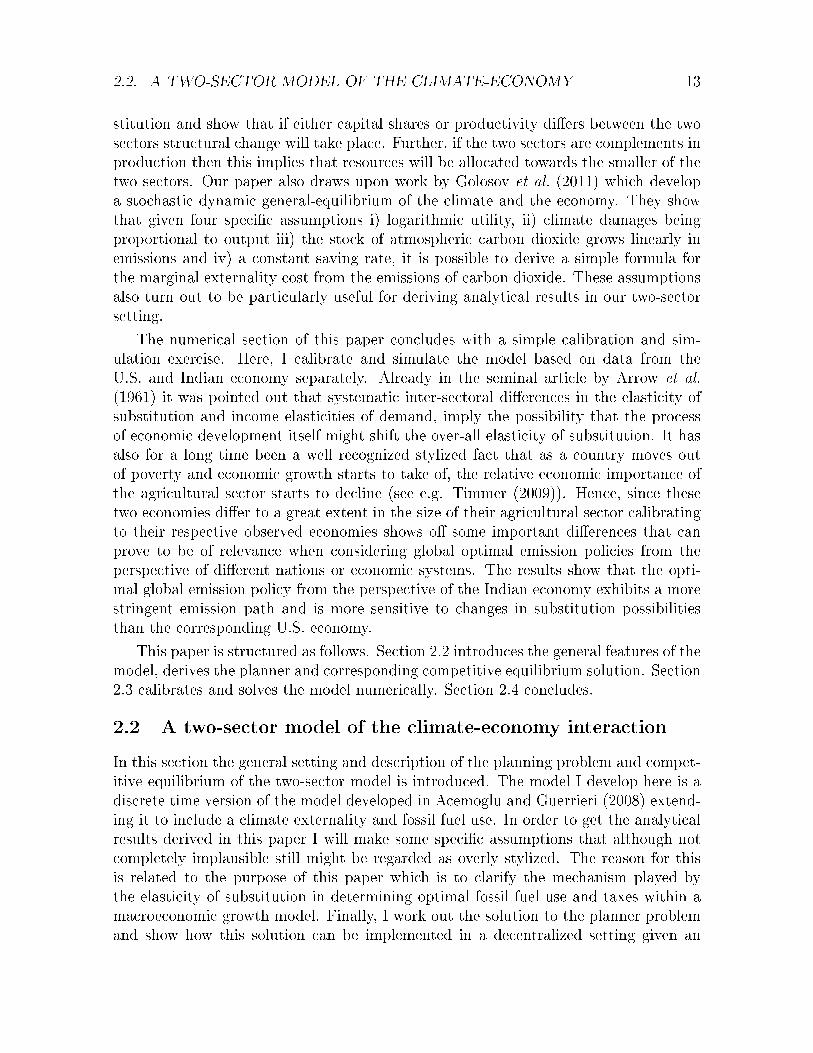
2.2. A TWO-SECTOR MODEL OF THE CLIMATE-ECONOMY 13
stitution and show that if either capital shares or productivity diers between the twosectors structural change will take place. Further, if the two sectors are complements inproduction then this implies that resources will be allocated towards the smaller of thetwo sectors. Our paper also draws upon work by Golosov et al. (2011) which developa stochastic dynamic general-equilibrium of the climate and the economy. They showthat given four specic assumptions i) logarithmic utility, ii) climate damages beingproportional to output iii) the stock of atmospheric carbon dioxide grows linearly inemissions and iv) a constant saving rate, it is possible to derive a simple formula forthe marginal externality cost from the emissions of carbon dioxide. These assumptionsalso turn out to be particularly useful for deriving analytical results in our two-sectorsetting.
The numerical section of this paper concludes with a simple calibration and sim-ulation exercise. Here, I calibrate and simulate the model based on data from theU.S. and Indian economy separately. Already in the seminal article by Arrow et al.(1961) it was pointed out that systematic inter-sectoral dierences in the elasticity ofsubstitution and income elasticities of demand, imply the possibility that the processof economic development itself might shift the over-all elasticity of substitution. It hasalso for a long time been a well recognized stylized fact that as a country moves outof poverty and economic growth starts to take of, the relative economic importance ofthe agricultural sector starts to decline (see e.g. Timmer (2009)). Hence, since thesetwo economies dier to a great extent in the size of their agricultural sector calibratingto their respective observed economies shows o some important dierences that canprove to be of relevance when considering global optimal emission policies from theperspective of dierent nations or economic systems. The results show that the opti-mal global emission policy from the perspective of the Indian economy exhibits a morestringent emission path and is more sensitive to changes in substitution possibilitiesthan the corresponding U.S. economy.
This paper is structured as follows. Section 2.2 introduces the general features of themodel, derives the planner and corresponding competitive equilibrium solution. Section2.3 calibrates and solves the model numerically. Section 2.4 concludes.
2.2 A two-sector model of the climate-economy interaction
In this section the general setting and description of the planning problem and compet-itive equilibrium of the two-sector model is introduced. The model I develop here is adiscrete time version of the model developed in Acemoglu and Guerrieri (2008) extend-ing it to include a climate externality and fossil fuel use. In order to get the analyticalresults derived in this paper I will make some specic assumptions that although notcompletely implausible still might be regarded as overly stylized. The reason for thisis related to the purpose of this paper which is to clarify the mechanism played bythe elasticity of substitution in determining optimal fossil fuel use and taxes within amacroeconomic growth model. Finally, I work out the solution to the planner problemand show how this solution can be implemented in a decentralized setting given an
14 CHAPTER 2. STRUCTURAL AND CLIMATIC CHANGE
externality correcting taxation policy.
2.2.1 Model description
The objective function of a representative household in the economy is given by
∞∑t=0
βtU(Ct) (2.1)
where U is a standard concave the utility function function, C consumption and β ∈(0, 1) is the discount factor.
The economy produces a unique nal good which can be thought of as an aggre-gate/composite good consisting of the two intermediate goods
Yt =(wmY
(ε−1)/εmt + waY
(ε−1)/εat
)ε/(ε−1)
(2.2)
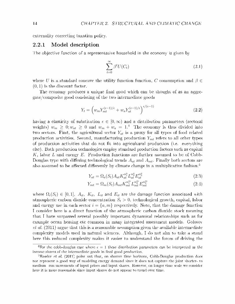
having a elasticity of substitution ε ∈ [0,∞) and a distribution parameters (sectoralweights) wm ≥ 0;wat ≥ 0 and wm + wa = 1.4 The economy is thus divided intotwo sectors. First, the agricultural sector Yat is a proxy for all types of food relatedproduction activities. Second, manufacturing production Ymt refers to all other typesof production activities that do not t into agricultural production (i.e. everythingelse). Both production technologies employ standard production factors such as capitalK, labor L and energy E. Production functions are further assumed to be of Cobb-Douglas type with diering technological trends Aat and Amt. Finally both sectors arealso assumed to be aected dierently by climate change in a multiplicative fashion.5
Yat = Ωa(St)AatKαa1at L
αa2at E
αa3at (2.3)
Ymt = Ωm(St)AmtKαm1mt L
αm2mtE
αm3mt (2.4)
where Ωi(St) ∈ [0, 1], Ait, Kit, Lit and Eit are the damage function associated withatmospheric carbon dioxide concentration St > 0, technological growth, capital, laborand energy use in each sector i = a,m respectively. Note, that the damage functionI consider here is a direct function of the atmospheric carbon dioxide stock meaningthat I have surpassed several possibly important dynamical relationships such as forexample ocean heating etc common in many integrated assessment models. Golosovet al. (2011) argue that this is a reasonable assumption given the available intermediatecomplexity models used in natural sciences. Although, I do not aim to take a standhere this reduced complexity makes it easier to understand the forces of driving the
4For the cobb-douglas case where ε = 1 these distribution parameters can be interpreted as theincome shares of the intermediate goods in nal good production.
5Hassler et al. (2011) point out that, on shorter time horizons, Cobb-Douglas production doesnot represent a good way of modeling energy demand since it does not capture the joint shorter- tomedium- run movements of input prices and input shares. However, on longer time scale we considerhere it is more reasonable since input shares do not appear to trend over time.

2.2. A TWO-SECTOR MODEL OF THE CLIMATE-ECONOMY 15
model we consider here.6 Further, I will throughout this paper assume that damagesare always increasing in the atmospheric carbon stock i.e. Ω
′i(St) < 0.
Finally, the economy's budget constraint in nal good production is
Kt+1 + Ct = Yt + (1− δ)Kt (2.5)
where the left hand side denotes next periods resource use (capital and consumption)while the right hand side denotes production and depreciation of capital.
Regarding fossil fuel use dynamics let Rt denote the stock of remaining fossil fuelat the beginning of time period t, where R0 > 0 is given, and Et ≥ 0 denotes the totalamount of extracted fossil fuel by the two sectors.
Rt+1 −Rt = −Et, R(0) = R0 > 0 (2.6)
the following resource constraint thus applies:
R0 ≥∞∑t=0
Et (2.7)
Capital, Labor and Energy can be allocated costlessly across both sectors. Marketclearing thus requires that
Kt = Kat +Kmt (2.8a)Lt = Lat + Lmt (2.8b)Et = Emt + Eat (2.8c)
Finally, I let St denote the stock of carbon dioxide emitted after the pre-industrialperiod and assume the following simple structure for the carbon cycle.
St+1 = (1− ϕ)St + ξEt (2.9)
This equation is a much simplied expression for the behavior of anthropogenic inducedCO2 emissions following early work on climate economy models (see e.g. Nordhaus(1994)) where ϕ captures the rate of removal of CO2 from the atmosphere and ξ theairborne fraction of carbon dioxide emissions. Removal might be due to for exampleuptake by oceans or the terrestrial biosphere. This is a rather simple an crude way ofcapturing carbon storage which ignores several possibly important dynamical relation-ships present in for example Nordhaus and Boyer (2000). However, for the purposes ofthe present paper these dynamics serve us well as a simplied representation. Further,as a reference Golosov et al. (2011) argue that increased complexity of the three boxcarbon cycle used by Nordhaus is quite well approximated by a simple one-dimensionallag structure.
6In the numerical section of this paper I will make a simple logarthmic transformation from carbondioxide to temperature units found in e.g. IPCC (2001).

16 CHAPTER 2. STRUCTURAL AND CLIMATIC CHANGE
2.2.2 The Planning problem
Based on the formulations described above I can now form a social planner problemand characterize a solution. The planner problem becomes
maxKt+1,Rt+1,St+1Et,Ct,Kmt,Kat,Lat,Lmt,Emt,Eat
∞∑t=0
βtU(Ct) (2.10)
subject to (2.2), (2.3) (2.4), (2.5), (2.6), (2.8a), (2.8b), (2.8c), (2.9) (2.11)
Inspection of the social planner problem reveals that this maximization problem can bebroken down into two parts. First, given the state variables Kt, Rt and St the allocationof factors across the two sectors becomes an intratemporal problem of maximizing theaggregate output Yt in each time period. Second, given this choice of factor allocationin each time period the time path of Ct and Et can be chosen so as to maximize thevalue of the objective function. These two parts thus corresponds to the solutions ofthe static and dynamic maximization problems. I start by characterizing the staticequilibrium.
Static equilibrium
As mentioned previously, in order to obtain a tractable model in terms of analyticalresults I will have to make some rather specic assumptions. The rst assumptionrelates to the factor input shares within the two sectors
Assumption 2.1. αaj = αmj ≡ αj, for j = 1, 2, 3
This assumption is crucial in order to obtain the analytical results derived below. Ideviate in this respect from the model derived in Acemoglu and Guerrieri (2008) whichrelies on diering input shares generating sectoral reallocations. However, as will beseen this assumption serves us well as a baseline case and will help us esh out themechanisms that are driving our results. Based on this assumption it is clear thatoptimal resource allocation will require that the marginal products of capital labor andenergy are equalized:
wmα1
(YtYmt
) 1ε YmtKmt
= waα1
(YtYat
) 1ε YatKat
wmα2
(YtYmt
) 1ε YmtLmt
= waα2
(YtYat
) 1ε YatLat
wmα3
(YtYmt
) 1ε YmtEmt
= waα3
(YtYat
) 1ε YatEat
(2.12)
Based on these equations I can solve for the optimal capital, labor and energy sharesallocated to each sector. This is allocation is given by the following proposition.
2.2. A TWO-SECTOR MODEL OF THE CLIMATE-ECONOMY 17
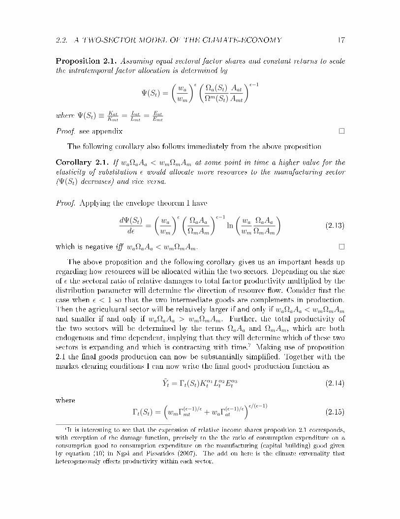
Proposition 2.1. Assuming equal sectoral factor shares and constant returns to scalethe intratemporal factor allocation is determined by
Ψ(St) =
(wawm
)ε(Ωa(St)
Ωm(St)
AatAmt
)ε−1
where Ψ(St) ≡ KatKmt
= LatLmt
= EatEmt
Proof. see appendix
The following corollary also follows immediately from the above proposition
Corollary 2.1. If waΩaAa < wmΩmAm at some point in time a higher value for theelasticity of substitution ε would allocate more resources to the manufacturing sector(Ψ(St) decreases) and vice versa.
Proof. Applying the envelope theorem I have
dΨ(St)
dε=
(wawm
)ε(ΩaAaΩmAm
)ε−1
ln
(wawm
ΩaAaΩmAm
)(2.13)
which is negative i waΩaAa < wmΩmAm.
The above proposition and the following corollary gives us an important heads upregarding how resources will be allocated within the two sectors. Depending on the sizeof ε the sectoral ratio of relative damages to total factor productivity multiplied by thedistribution parameter will determine the direction of resource ow. Consider rst thecase when ε < 1 so that the two intermediate goods are complements in production.Then the agricultural sector will be relatively larger if and only if waΩaAa < wmΩmAmand smaller if and only if waΩaAa > wmΩmAm. Further, the total productivity ofthe two sectors will be determined by the terms ΩaAa and ΩmAm, which are bothendogenous and time dependent, implying that they will determine which of these twosectors is expanding and which is contracting with time.7 Making use of proposition2.1 the nal goods production can now be substantially simplied. Together with themarket clearing conditions I can now write the nal goods production function as
Yt = Γt(St)Kα1t Lα2
t Eα3t (2.14)
whereΓt(St) =
(wmΓ
(ε−1)/εmt + waΓ
(ε−1)/εat
)ε/(ε−1)
(2.15)
7It is interesting to see that the expression of relative income shares proposition 2.1 corresponds,with exception of the damage function, precisely to the the ratio of consumption expenditure on aconsumption good to consumption expenditure on the manufacturing (capital building) good givenby equation (10) in Ngai and Pissarides (2007). The add on here is the climate externality thatheterogeneously eects productivity within each sector.

18 CHAPTER 2. STRUCTURAL AND CLIMATIC CHANGE
and
Γat = Ωa(St)Aat
(Ψ(St)
1 + Ψ(St)
)(2.16)
Γmt = Ωm(St)Amt
(1
1 + Ψ(St)
)(2.17)
As can be seen from the above equations the solution to the static equilibrium willsimplify the dynamic analysis greatly since nal goods production is now a function ofonly carbondioxide S and the aggregate resource inputs K,L,E.Dynamic equilibrium
In order to proceed with analytical results also in derivation of the dynamic equilibriumI will also assume that utility is logarithmic and a capital depreciation rate of a hundredpercent.
Assumption 2.2. U(Ct) = ln(Ct), δ = 1
Logarithmic preferences is rather standard and a common assumption in many mod-els. For example, the earlier climate economy models developed by William Nordhausall featured logarithmic preferences (see e.g. Nordhaus (1994); Nordhaus and Boyer(2000)). As the main purpose of this paper is more qualitative than quantitative innature I will not spend time on discussing the robustness of the results to this assump-tion. However, judging from the results derived in this paper and based on the work ofAcemoglu and Guerrieri (2008)8, modifying this assumption should not aect the qual-itative results derived here regarding structural transformation. Golosov et al. (2011)also use and discuss these assumptions. They argue that in particular for longer timeperiods (10 years) suggests a lower curvature of the utility function.
A depreciation rate of a hundred percent is large even for a ten year period. Golosovet al. (2011) claim that this does not aect the results of their model remarkably.Together these assumptions are convenient in these types models since it is well knownthat as long as aggregate capital can be factored out of the production function thesaving rate will become a constant.9
Given this assumption and the results derived from the static equilibrium we cannow write down the lagrangian of the dynamic problem facing the social planner
L =∞∑t=0
βt[ln(Yt −Kt+1) + λRt(Rt − Et −Rt+1) + λSt((1− ϕ)St + Et − St+1)] (2.18)
Taking the F.O.C w.r.t. Kt+1 we have
LKt+1 = −βt1
Ct+ βt+1
1
Ct+1
α1YtKt+1
= 0 (2.19)
8In particular, see proposition 1 and 2 of this paper.9This assumption was rst used by Brock and Mirman (1972) to provide a closed-form solution in
a stochastic growth setting.

2.2. A TWO-SECTOR MODEL OF THE CLIMATE-ECONOMY 19
which gives us
Ct+1
Ct= βα1
Yt+1
Kt+1
(2.20)
which gives us the following consumption/investment rule:
Ct = (1− βα1)Yt (2.21)
Kt+1 = βα1Yt (2.22)
From the above calculations we see that optimal investment in capital K remains axed fraction βα1 of manufacturing production over time. Hence it is unaected bychanges to the parameters in the instantaneous utility function such as the elasticity ofsubstitution ε between the two consumption goods.
Concerning optimal fuel use I now proceed with the rst order conditions w.r.t. thefossil fuel:
LRt+1 = −βtλRt + βt+1λRt+1 = 0 (2.23)
LEt = α31
Ct
YtEt− λRt + λSt = 0 (2.24)
LSt+1 = βt+1 1
Ct+1
∂Γt+1
∂St+1
Kα1t+1L
α2t+1E
α3t+1 − βtλSt + βt+1λSt+1(1− ϕ) = 0 (2.25)
From (2.25) we have:
λSt = β1
Ct+1
∂Γt+1
∂St+1
Yt+1
Γt+1
+ βλSt+1(1− ϕ)
and thus
λSt =∞∑s=1
(1− ϕ)s−1βs
(1
Ct+s
∂Γt+s∂St+s
Yt+sΓt+s
)+ lim
s→∞(1− ϕ)s−1βs
(1
Ct+s
∂Γt+s∂St+s
Yt+sΓt+s
)(2.26)
By the transversality condition the limiting term is zero and if we express the marginaldamage cost λSt in terms of present day consumption ΛSt ≡ λSt/U
′(Ct) we get an
expression similar to equation (12) of Golosov et al. (2011).
ΛSt =∞∑s=1
(1− ϕ)s−1βs
(CtYt+sCt+s
∂Γt+s∂St+s
1
Γt+s
)(2.27)
This formula is more complex than the one derived in their paper. In particular theformula does not depend on merly the saving rate but also on fossil fuel use thru theterm ∂Γt+s
∂St+s1
Γt+swhich I will refer to as the "relative damage term". However, as will

20 CHAPTER 2. STRUCTURAL AND CLIMATIC CHANGE
be shown in the next section this term is not a complete black box and we can learnalot about its properties by analyzing how it is aected by changes in its parameters.Further, if we express the marginal externality costs of emissions as a proportion of GDPi.e. ΛSt ≡ ΛSt/Yt and make use of the consumption rule we get a simpler expressionwhich is independent of saving and well suited for examining the role of the elasticityof substitution for climate damages.
ΛSt =∞∑s=1
(1− ϕ)s−1βs(∂Γt+s∂St+s
1
Γt+s
)(2.28)
The marginal externality cost of CO2 and the elasticity of substitution
From (2.2.2) we saw how allocation of factor inputs depended on technical and climaticchange within the two sectors and the role played by the elasticity of substitution. Inexpression (2.28) we see that marginal climate damages also depends on the elastic-tity of substitution through the relative damage term ∂Γt+s
∂St+s1
Γt+s. Hence the marginal
externality cost of atmospheric carbon dioxide will depend upon both the substitutionpossibilities amongst the two sectors and how damages are spread between them. Thefollowing proposition is usefull in order to understand how this works.
Proposition 2.2. For 0 ≤ ε < ∞ the marginal externality cost of carbon dioxide perunit of GDP (2.28) is always negative and bounded above and below by the marginaldamages within each sector.
ΛSt(ε) ∈[ΛSt(0), ΛSt(∞)
](2.29)
where
ΛSt(0) =∞∑s=1
(1− ϕ)s−1βs(ΩaAat)
−1 Ω′a
Ωa+ ΩmAmt)
−1 Ω′m
Ωm
(ΩmAmt)−1 + (ΩaAat)−1
(2.30)
ΛSt(∞) =
∑∞s=1(1− ϕ)s−1βsΩ
′a
Ωaif waΩaAa > wmΩmAm∑∞
s=1(1− ϕ)s−1βsΩ′m
Ωmif waΩaAa < wmΩmAm
(2.31)
there are four cases to consider:
i) waΩaAa > wmΩmAm andΩ′a
Ωa
<Ω′m
Ωm
then ΛSt(∞) < ΛSt(0) : ΛSt decreasing in ε
ii) waΩaAa > wmΩmAm andΩ′a
Ωa
>Ω′m
Ωm
then ΛSt(∞) > ΛSt(0) : ΛSt increasing in ε
iii) waΩaAa < wmΩmAm andΩ′a
Ωa
<Ω′m
Ωm
then ΛSt(∞) > ΛSt(0) : ΛSt increasing in ε
iv) waΩaAa < wmΩmAm andΩ′a
Ωa
>Ω′m
Ωm
then ΛSt(∞) < ΛSt(0) : ΛSt decreasing in ε
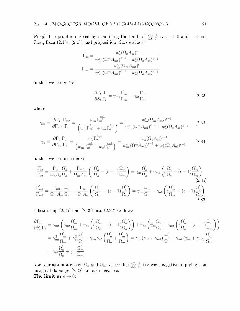
2.2. A TWO-SECTOR MODEL OF THE CLIMATE-ECONOMY 21
Proof. The proof is derived by examining the limits of ∂Γt∂St
1Γt
as ε → 0 and ε → ∞.First, from (2.16), (2.17) and proposition (2.1) we have
Γat =wεa(ΩaAat)
ε
wεm (ΩmAmt)ε−1 + wεa(ΩaAat)ε−1
Γmt =wεm(ΩmAmt)
ε
wεm (ΩmAmt)ε−1 + wεa(ΩaAat)ε−1
further we can write
∂Γt∂St
1
Γt= γmt
Γ′mt
Γmt+ γat
Γ′at
Γat(2.32)
where
γm ≡∂Γt∂Γmt
ΓmtΓt
=wmΓ
ε−1ε
m(wmΓ
ε−1ε
m + waΓε−1ε
a
) =wεm(ΩmAmt)
ε−1
wεm (ΩmAmt)ε−1 + wεa(ΩaAat)ε−1
(2.33)
γa ≡∂Γt∂Γat
ΓatΓt
=waΓ
ε−1ε
a(wmΓ
ε−1ε
m + waΓε−1ε
a
) =wεa(ΩaAat)
ε−1
wεm (ΩmAmt)ε−1 + wεa(ΩaAat)ε−1
(2.34)
further we can also derive
Γ′at
Γat=
ΓatΩaAa
Ω′a
Ωa
+Γmt
ΩmAm
(εΩ′a
Ωa
− (ε− 1)Ω′m
Ωm
)= γat
Ω′a
Ωa
+ γmt
(εΩ′a
Ωa
− (ε− 1)Ω′m
Ωm
)(2.35)
Γ′mt
Γmt=
ΓmtΩmAm
Ω′m
Ωm
+Γat
ΩaAa
(εΩ′m
Ωm
− (ε− 1)Ω′a
Ωa
)= γmt
Ω′m
Ωm
+ γat
(εΩ′m
Ωm
− (ε− 1)Ω′a
Ωa
)(2.36)
substituting (2.35) and (2.36) into (2.32) we have
∂Γt∂St
1
Γt= γmt
(γmt
Ω′m
Ωm
+ γat
(εΩ′m
Ωm
− (ε− 1)Ω′a
Ωa
))+ γat
(γat
Ω′a
Ωa
+ γmt
(εΩ′a
Ωa
− (ε− 1)Ω′m
Ωm
))= γ2
mt
Ω′m
Ωm
+ γ2at
Ω′a
Ωa
+ γmtγat
(Ω′a
Ωa
+Ω′m
Ωm
)= γat (γat + γmt)
Ω′a
Ωa
+ γmt (γat + γmt)Ω′m
Ωm
= γatΩ′a
Ωa
+ γmtΩ′m
Ωm
from our assumptions on Ωa and Ωm we see that ∂Γt∂St
1Γt
is always negative implying thatmarginal damages (2.28) are also negative.The limit as ε→ 0:
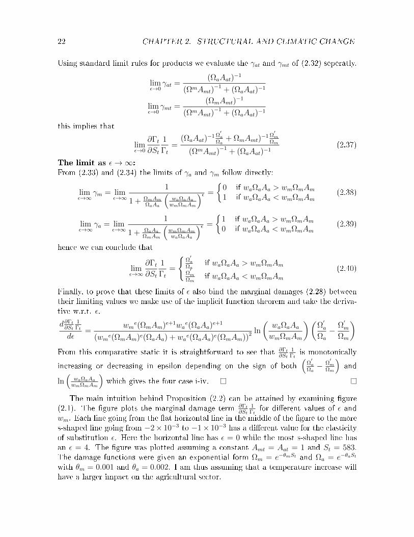
22 CHAPTER 2. STRUCTURAL AND CLIMATIC CHANGE
Using standard limit rules for products we evaluate the γat and γmt of (2.32) seperatly.
limε→0
γat =(ΩaAat)
−1
(ΩmAmt)−1 + (ΩaAat)−1
limε→0
γmt =(ΩmAmt)
−1
(ΩmAmt)−1 + (ΩaAat)−1
this implies that
limε→0
∂Γt∂St
1
Γt=
(ΩaAat)−1 Ω
′a
Ωa+ ΩmAmt)
−1 Ω′m
Ωm
(ΩmAmt)−1 + (ΩaAat)−1
(2.37)
The limit as ε→∞:From (2.33) and (2.34) the limits of γa and γm follow directly:
limε→∞
γm = limε→∞
1
1 + ΩmAmΩaAa
(waΩaAawmΩmAm
)ε =
0 if waΩaAa > wmΩmAm1 if waΩaAa < wmΩmAm
(2.38)
limε→∞
γa = limε→∞
1
1 + ΩaAaΩmAm
(wmΩmAmwaΩaAa
)ε =
1 if waΩaAa > wmΩmAm0 if waΩaAa < wmΩmAm
(2.39)
hence we can conclude that
limε→∞
∂Γt∂St
1
Γt=
Ω′a
Ωaif waΩaAa > wmΩmAm
Ω′m
Ωmif waΩaAa < wmΩmAm
(2.40)
Finally, to prove that these limits of ε also bind the marginal damages (2.28) betweentheir limiting values we make use of the implicit function theorem and take the deriva-tive w.r.t. ε.
d∂Γt∂St
1Γt
dε=
wme(ΩmAm)e+1wa
e(ΩaAa)e+1
(wme(ΩmAm)e(ΩaAa) + wae(ΩaAa)e(ΩmAm))2 ln
(waΩaAawmΩmAm
)(Ω′a
Ωa
− Ω′m
Ωm
)From this comparative static it is straightforward to see that ∂Γt
∂St1Γt
is monotonically
increasing or decreasing in epsilon depending on the sign of both(
Ω′a
Ωa− Ω
′m
Ωm
)and
ln(
waΩaAawmΩmAm
)which gives the four case i-iv.
The main intuition behind Proposition (2.2) can be attained by examining gure(2.1). The gure plots the marginal damage term ∂Γt
∂St1Γt
for dierent values of ε andwm. Each line going from the at horizontal line in the middle of the gure to the mores-shaped line going from −2× 10⁻³ to −1× 10⁻³ has a dierent value for the elasticityof substitution ε. Here the horizontal line has ε = 0 while the most s-shaped line hasan ε = 4. The gure was plotted assuming a constant Amt = Aat = 1 and St = 583.The damage functions were given an exponential form Ωm = e−θmSt and Ωa = e−θaSt
with θm = 0.001 and θa = 0.002. I am thus assuming that a temperature increase willhave a larger impact on the agricultural sector.

2.2. A TWO-SECTOR MODEL OF THE CLIMATE-ECONOMY 23
0 0.1 0.2 0.3 0.4 0.5 0.6 0.7 0.8 0.9 1−2
−1.9
−1.8
−1.7
−1.6
−1.5
−1.4
−1.3
−1.2
−1.1
−1x 10
−3
wm
∂Γ
t
∂S
t
1 Γt
Figure 2.1: Behaviour of the relative damage term (∂Γt∂St
1Γt) for dierent values of ε and
wm. Flatter lines depict small values of ε while increasing s-shaped correspond to highervalues of ε. The gure was plotted assuming a constant Amt = Aat = 1 and St = 583.The damage functions were given an exponential form Ωm = e−θmSt and Ωa = e−θaSt
with θm = 0.001 and θa = 0.002.
The gure conrms the results of Proposition (2.2). For an elasticity of substitutionequal to zero the marginal damage term is merely a weighted average of the marginaldamages within each sector which is independent of the distribution parameter. How-ever, as ε increases the marginal damage term moves towards the boundaries discussedin Proposition (2.2) where the direction depends on the conditions i − iv. Numericalexamination of the behavior when ε → ∞ shows that the steepness of the s-shapeincreases with an increasing ε with a threshold located about the dashed vertical line.
Concerning the interpretation, there are two cases to consider. First, consider thecase where wm lies in the region to the right of the dashed vertical line in gure 2.1. Inthis case we can see from the gure that for each xed value of wm the relative damageterm increases with higher values of ε. Hence, judging from proposition (2.2) we canconclude that this should correspond to the case where waΩaAa < wmΩmAm. Further,by proposition (2.1) we also see that in this case resources are moving in the directionof the manufacturing sector and since a large value of ε corresponds to a high degree ofsubstitutability this simply means that we are allocating more resources to the sectorwhich suers the least by climate change.
The second case corresponds to small values of wm lying to the right of the dashed
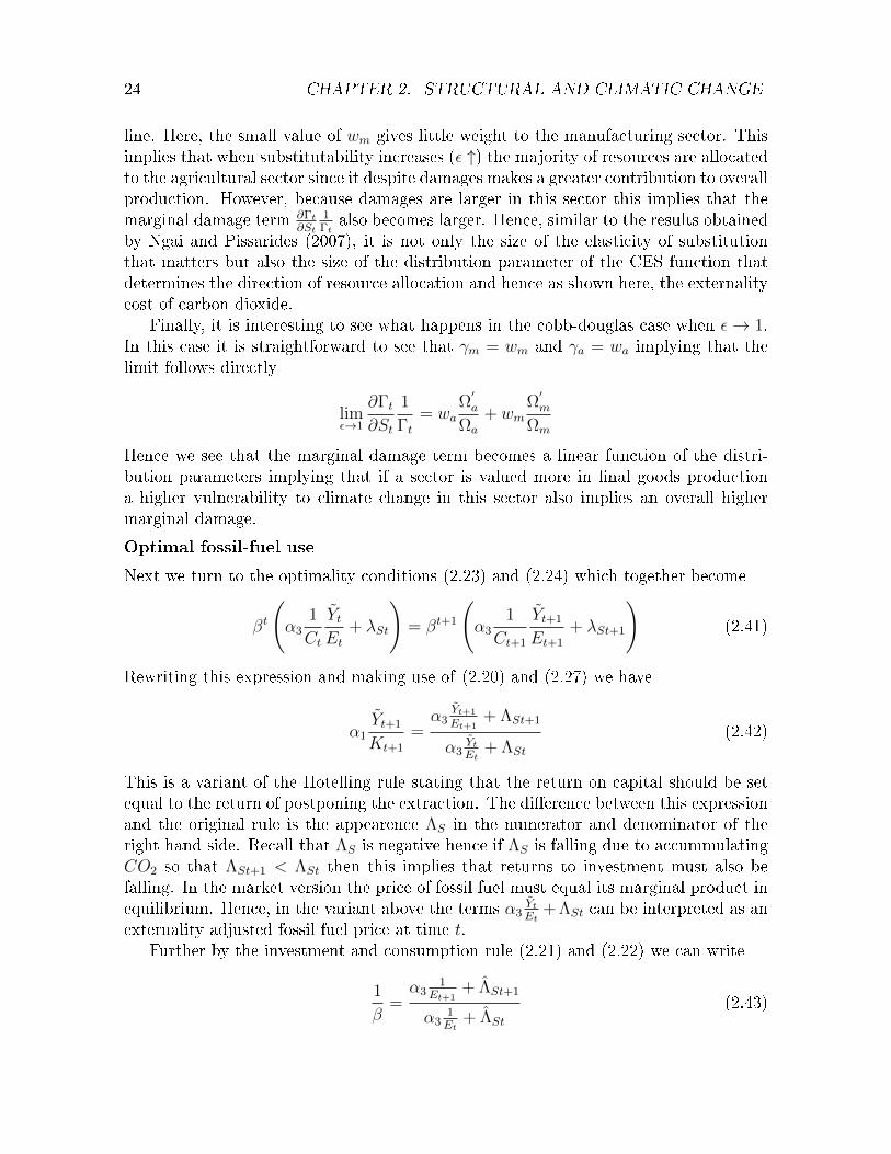
24 CHAPTER 2. STRUCTURAL AND CLIMATIC CHANGE
line. Here, the small value of wm gives little weight to the manufacturing sector. Thisimplies that when substitutability increases (ε ↑) the majority of resources are allocatedto the agricultural sector since it despite damages makes a greater contribution to overallproduction. However, because damages are larger in this sector this implies that themarginal damage term ∂Γt
∂St1Γt
also becomes larger. Hence, similar to the results obtainedby Ngai and Pissarides (2007), it is not only the size of the elasticity of substitutionthat matters but also the size of the distribution parameter of the CES function thatdetermines the direction of resource allocation and hence as shown here, the externalitycost of carbon dioxide.
Finally, it is interesting to see what happens in the cobb-douglas case when ε→ 1.In this case it is straightforward to see that γm = wm and γa = wa implying that thelimit follows directly
limε→1
∂Γt∂St
1
Γt= wa
Ω′a
Ωa
+ wmΩ′m
Ωm
Hence we see that the marginal damage term becomes a linear function of the distri-bution parameters implying that if a sector is valued more in nal goods productiona higher vulnerability to climate change in this sector also implies an overall highermarginal damage.
Optimal fossil-fuel use
Next we turn to the optimality conditions (2.23) and (2.24) which together become
βt
(α3
1
Ct
YtEt
+ λSt
)= βt+1
(α3
1
Ct+1
Yt+1
Et+1
+ λSt+1
)(2.41)
Rewriting this expression and making use of (2.20) and (2.27) we have
α1Yt+1
Kt+1
=α3
Yt+1
Et+1+ ΛSt+1
α3YtEt
+ ΛSt
(2.42)
This is a variant of the Hotelling rule stating that the return on capital should be setequal to the return of postponing the extraction. The dierence between this expressionand the original rule is the appearence ΛS in the numerator and denominator of theright hand side. Recall that ΛS is negative hence if ΛS is falling due to accummulatingCO2 so that ΛSt+1 < ΛSt then this implies that returns to investment must also befalling. In the market version the price of fossil fuel must equal its marginal product inequilibrium. Hence, in the variant above the terms α3
YtEt
+ ΛSt can be interpreted as anexternality adjusted fossil fuel price at time t.
Further by the investment and consumption rule (2.21) and (2.22) we can write
1
β=α3
1Et+1
+ ΛSt+1
α31Et
+ ΛSt
(2.43)

2.2. DECENTRALIZED EQUILIBRIUM 25
We can now see how a constant saving rate greatly simplies the analysis. As canbe seen from (2.43) the optimal path of fossil fuel use can now be fully determinedgiven the appropriate end constraints and that carbon dioxide accumulation dependson past values of emissions according to (2.9). Hence, the decision regarding capitalaccumulation has been separated out from that evolving energy use.
2.2.3 Decentralized equilibrium
I will now characterize the how the optimum can be implemented using either a ad-valorem (τt) or a per-unit taxes (θt). I assume that the government taxes resources rmsin order to implement the optimum. Consider rst the problem of the the representivehousehold/individual problem
max∞∑t=0
βtU(Ct),
s.t. Ct +Kt+1 = rtKt + wt + Πet +Gt (2.44)
as usual households are assumed to own both production and resource extraction rmsand hence prot by renting out capital at the rate rt, labor at the wage rate wt, protsfrom resource extraction Πe
t ≡ (pEt − θt)(1 − τt)Et and government transfers Gt ≡τtpEtEt + θtEt where pEt denotes the before tax price on fossil fuel. The f.o.c. for Kt+1
is
Ct+1
Ct= βrt+1 (2.45)
Second, the representative rm within the each sector faces the following problem
maxKit,Lit,Eit
pyitYit − rtKit − wtLit − pEtEit, ∀i ∈ m, a
with the f.o.c. given by
rt = pyit∂Yt∂Kit
, wt = pyit∂Yt∂Lit
, pEt = pyit∂Yt∂Emt
(2.46)
Final good production is also done under prot maximization and perfect competitionimplying that the marginal product of each good will equal its price. Normalizing theprice of the nal good to one we thus have that:
pyit = wi
(YtYit
) 1ε
(2.47)

26 CHAPTER 2. STRUCTURAL AND CLIMATIC CHANGE
inserting this into (2.46) we see that
rt = wm
(YtYmt
) 1ε ∂Yt∂Kmt
= wa
(YtYat
) 1ε ∂Yt∂Kat
wt = wm
(YtYmt
) 1ε ∂Yt∂Lmt
= wa
(YtYat
) 1ε ∂Yt∂Lat
pEt = wm
(YtYmt
) 1ε ∂Yt∂Emt
= wa
(YtYat
) 1ε ∂Yt∂Eat
These prot maximizing conditions are the same as in the planner solution with thesolution derived in appendix and stated explicitly in (2.14). From this solution we thusknow that:
rt =∂Yt∂Kt
=∂Yt∂Kmt
= α1Γt(St)Kα1−1t Lα2
t Eα3t (2.48)
which implies that the same consumption/investment rules will apply as in the socialplanner solution i.e. (2.21) and (2.22) hold also in the decentralized solution.
Third, the representive resource extraction rm solves the problem
maxRt+1
∞∑t=0
(pEt − θt)(1− τt)Et
(t∏
s=0
rs
)−1
s.t. Rt+1 −Rt = −Et, Rt+1 ≥ 0
Once again, this gives us a hotelling type of formula
rt+1 =(pEt+1 − θt+1)(1− τt+1)
(pEt − θt)(1− τt)(2.49)
I have now characterized the decentralized solution. Next, in order to implement theplanning solution we have to set the private return of not using fossil fuels equal to itssocial return.
Proposition 2.3. The optimal tax can be implemented by either setting
θt = −Λst and τt = τ ∀tor by setting
τt = − Λst
∂Yt/∂Etand θt = 0
Proof. Setting the rental price of capital from (2.49) equal to that of the marginalproduct of capital in from the planner problem (2.42) we can write
(pEt+1 − θt+1)(1− τt+1)
(pEt − θt)(1− τt)=α3
Yt+1
Et+1+ ΛSt+1
α3YtEt
+ ΛSt
from this expression its immediate that if τt = τ then θt = Λst implements the planneroptimum. Likewise, if θt = 0 then τt = Λst
∂Yt/∂Etimplements the optimum.

2.3. NUMERICAL ANALYSIS 27
2.3 Numerical analysis
In this section I undertake a simple calibration and simulation exercise in order toillustrate how the optimal fossil fuel consumption problem is aected by underlyingmodel assumptions. I have chosen to calibrate two sets of parameter estimates based ondata from India and the U.S. economy respectively. These countries dier vastly in thesize of their agricultural sector compared to other sectors of the economy and thus serveswell as illustrative examples of economies having dierent sectoral compositions.10 Theresult of this calibration excercise can thus be seen as the policy suggestion resultingfrom two types of planners trying to adress the economic realities adherent in twoeconomies under dierent levels of economic development.11
2.3.1 Model calibration
In the analytical section above I neglected that economic damages from climate changeare typically measured as a function of temperature. This was done in order to avoidcomplexity that does not impact on qualitative modeling results. A simple way to cor-rect for this simplication is thru the Arrhenius equation, after the Swedish physicistSvante Arrhenius (1859-1927), which states that when CO2 increases in a geometricprogression, the augmentation of the temperature will increase in a nearly arithmeticprogression (see e.g. IPCC (2001)). This fairly simple way of capturing the relationshipbetween CO2 is still in use today in simplied climate system representations approxi-mating global temperature rise from a doubling of atmospheric CO2 (see e.g. Nordhaus(2007))
Tt ≡ T (St) = λ ln
(1 +
StS
)/ ln 2
where S is the pre-industrial atmospheric CO2 level and λ is a climate sensitivity param-eter. Following Nordhaus (2007) (see page 13) I assume a preindustrial concentration ofcarbon dioxide of S ≈ 596Gtc (gigagtons of carbon).12 Taking the fairly standard valueof 3 for λ we have that for a doubling of CO2 in the atmosphere temperature will riseby approximately 3 degrees Celsius.13 Tans (2011) reports a current CO2 concentrationas of December 2011 of 831Gtc. Hence, using the above formula this implies that global
10For example, the world bank estimates that agricultures share of value added amounts to ap-proximately 1% of the U.S. economy while in India the share is approximatly 20% (http://data.worldbank.org/indicator/NV.AGR.TOTL.ZS?page=1).
11It should be noted that the assumption of a constant elasticity of substitution is not uncontrover-sial. Already in the seminal article Arrow et al. (1961) it was pointed out that given the systematicinter-sectoral dierences in the elasticity of substitution and in income elasticities of demand, thepossibility arises that the process of economic development itself might shift the over-all elasticity ofsubstitution. Hence, estimates for the elasticity of substitution may vary greatly depending on thelevel of development.
12I report atmospheric carbon dioxide in gigatons of carbon (GtC) with a conversion factor 1 ppmby volume of atmospheric CO2 = 2.13 GtC.
13There is considerable uncertainty surrounding the appropriate estimate for climate sensitivity seefor example Roe and Baker (2007).

28 CHAPTER 2. STRUCTURAL AND CLIMATIC CHANGE
temperature has increased by approximately 1.44 degrees since pre-industrial levels lieswell in the ballpark of more accurate climate model runs found in e.g. the IPCC (2007).Concerning the carbon dioxide accumulation equation (2.9) two parameters need to becalibrated. First, the so called airborne fraction ξ which is the fraction of anthropogeniccarbon dioxide emissions that remain in the atmosphere. I model this fraction as con-stant hence assuming that there is no trend in the biosphere's and oceans ability toabsorb human induced emissions. Based on a recent study by Knorr (2009) I set theairborne fraction ξ = 0.43.14 Second, the parameter ϕ captures the rate at which car-bon is absorbed by the deep oceans. Archer (2005) claims that "...75% of an excessatmospheric carbon concentration has a mean lifetime of 300 year and the remaining25% stays there forever". Although my simple carbon cycle is unable to account forthe 25% always remaining in the atmosphere by setting ϕ = 0.05 this implies that after300 years (30 periods) approximately 75% of the carbon dioxide has been removed.
Next, I need to specify the damage functions for the two sectors. Although thereexists a large and growing literature concerned with sector specic damages at the lo-cal scale it is dicult to nd similar assessments at the global scale. Reviewing andaggregating such studies is a large undertaking and lies beyond the scope of the cur-rent paper.15 I follow Nordhaus (2007) here and specify a simple quadratic damagefunction for each of the two sectors and rely upon the aggregation results found in hisaccompanying notes for my benchmark estimation.16 On page 24 of his accompanyingnotes he presents damage estimates in percent of GDP disaggregated into 12 geograph-ical regions and seven damage sectors including an estimate of catastrophic damages.These damage estimates are then aggregated, using output weights based on predicted2105 year's GDP levels, into a single estimate of GDP loss due to a 2.5 degree warmingof approximately 1.77%. The exact size of these weights are however not a supportedpart of the DICE model.17 Following, Nordhaus (2007) I proceed by calibrating twodierent quadratic damage functions for both the U.S. and Indian economy based onthe estimates found in his notes. For the U.S. economy he estimates an economic im-pact of 0.03% of GDP from the agricultural sector and 0.88% of GDP from the rest ofthe economy from a 2.5 degree warming. Similarly for the Indian economy he estimatesan economic impact of 0.32% of GDP from the agricultural sector and 2.75% of GDPfrom the rest of the economy. Based on these estimates the damage functions
Ωa(Tt) =1
1 + θaT 2t
, Ωm(Tt) =1
1 + θmT 2t
(2.50)
are calibrated for the U.S. and Indian economy where the parameters are calculated asθa = 0.0003/2.52 ≈ 4.8 × 10⁻⁵ and θm = 0.0088/2.52 ≈ 0.0014 for the U.S. economyand set to θa = 0.0032/2.52 ≈ 0.000512 and θm = 0.0275/2.52 ≈ 0.0044 for the Indianeconomy.
14Although there exists several studies have reported an apparent increasing trend in the airbornefraction the study by Knorr (2009) claim that this trend is statistically insignicant.
15See e.g. Tol (2009) for a review of such estimates.16See http://nordhaus.econ.yale.edu/Accom_Notes_100507.pdf17Personal communication with William Nordhaus.

2.3. NUMERICAL ANALYSIS 29
For the parameters of the agricultural and manufacturing production functions Ifollow Golosov et al. (2011) and set α1 = 0.3, α2 = 0.67 and α3 = 0.03 for botheconomies. These estimates are fairly standard for manufacturing or as average esti-mates for the entire economy. However, if land is considered a capital good, empiricalstudies point to a much larger estimate for the capital income share in the agriculturalsector. Valentinyi and Herrendorf (2008) estimate income shares of capital and labor atthe sectoral level for the US economy and nd that the capital share of the agriculturalsector is approximately 50% larger than the capital share of the aggregate economy. Fordeveloping countries the share is somewhat smaller (Irz and Roe, 2005). Concerningthe TFP growth rates, Martin and Mitra (2001) estimate that the overall growth rate ofTFP in manufacturing varies between 1.13% and 1.86% between 2.34% and 2.91% foragriculture for a sample of 50 countries between the years 1967-92. This is one of thefew global studies I could nd with the same sectoral disaggregation as I consider here.I thus use the mean of these intervals, i.e. gm = 0.015 and ga = 0.026, as my initialbenchmark estimates in both economies. It should however be noted that there is asignicant amount of disagreement in the literature whether this relatively high rate ofTFP growth in agriculture can continue also in the future. The spread of knowledge onthe productive use of pesticides and fertilizers in farming increased output considerablyin this sector during the second half of the 20th century but it is unclear whether thislevel of growth can continue at the same pace in the future due to e.g. biophysicalconstraints in plant life (Ruttan, 2002).
Concerning the elasticity of substitution and distribution parameters I calibratethese following Acemoglu and Guerrieri (2008). Since, Yit corresponds to the quantityproduced in sector i ∈ m, a the value of output (nominal value added) produced insector i follows from Y n
it ≡ pitYit where pit is given by equation (2.46). This implies thefollowing way of estimating these parameters using a simple linear regression by takingthe log of the ratio of sectoral nominal value added and real value added
ln
(Y nmt
Y nat
)= ln
(wmwa
)+ε− 1
εln
(YmtYat
)(2.51)
I estimate the above equation using data from the Groningen Growth and DevelopmentCentre (GGDC) 10-sector database for the years 1950-2005 for the U.S. and Indianeconomy. The data set contains annual series of value added, real value added, andpersons employed for 10 broad sectors of the economy (Timmer and de Vries, 2009). Ilet the agriculture, forestry, and shing sector of the 10 sector database represent theagricultural sector of my model while the aggregate of the remaining sectors excludinggovernment services serves as a proxy for the manufacturing sector. Using these aggre-gate estimates of real value added and value added I obtain by linear regression from(2.51) an estimate of ε ≈ 1.62 with a standard error of 0.147 for the U.S. economy. Forthe Indian economy the corresponding estimate is ε ≈ 2.13 with a standard error of0.15.18 I thus choose these values as my benchmark estimates and then calibrate wm
18Both estimates are signicant on the 1% level.
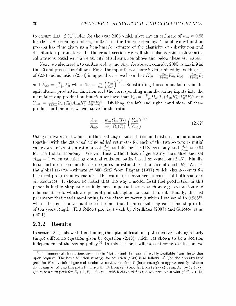
30 CHAPTER 2. STRUCTURAL AND CLIMATIC CHANGE
to ensure that (2.51) holds for the year 2005 which gives me an estimate of wm ≈ 0.95for the U.S. economy and wm ≈ 0.64 for the Indian economy. The above estimationprocess has thus given us a benchmark estimate of the elasticity of substitution anddistribution parameters. In the result section we will thus also consider alternativecalibrations based with an elasticity of substitution above and below these estimates.
Next, we also need a to calibrate Am0 and Aa0. As above I consider 2005 as the initialtime 0 and proceed as follows. First, the input factor share is determined by making useof (2.8) and equation (2.53) in appendix i.e. we have that Ka0 = Ψ0
1+Ψ0K0, La0 = Ψ0
1+Ψ0L0
and Ea0 = Ψ0
1+Ψ0E0 where Ψ0 ≡ wa
wm
(Ya0Ym0
) ε−1ε. Substituting these input factors in the
agricultural production function and the corresponding manufacturing inputs into themanufacturing production function we have that Ya0 = Ψ0
1+Ψ0Ωa(T0)Aa0K
α10 Lα2
0 Eα30 and
Ym0 = 11+Ψ0
Ωm(T0)Am0Kα10 Lα2
0 Eα30 . Dividing the left and right hand sides of these
production functions we can solve for the ratio
Aa0
Am0
=wmwa
Ωm(Tt)
Ωa(Tt)
(Ya0
Ym0
)1/ε
(2.52)
Using our estimated values for the elasticity of substitution and distribution parameterstogether with the 2005 real value added estimates for each of the two sectors as initialvalues we arrive at an estimate of Aa0
Am0≈ 1.46 for the U.S. economy and Aa0
Am0≈ 0.94
for the Indian economy. We can thus without loss of generality normalize and setAm0 = 1 when calculating optimal emission paths based on equation (2.43). Finally,fossil fuel use in our model also requires an estimate of the current stock R0. We usethe global reserve estimate of 5000GtC from Rogner (1997) which also accounts fortechnical progress in extraction. This estimate is assumed to consist of both coal andoil resources. It should be noted that the way I model fossil fuel production in thispaper is highly simplistic as it ignores important issues such as e.g. extraction andrenement costs which are generally much higher for coal than oil. Finally, the lastparameter that needs mentioning is the discount factor β which I set equal to 0.98510,where the tenth power is due to the fact that I am considering each time step to beof ten years length. This follows previous work by Nordhaus (2007) and Golosov et al.(2011).
2.3.2 Results
In section 2.2, I showed, that nding the optimal fossil fuel path involves solving a fairlysimple dierence equation given by equation (2.43) which was shown to be a decisionindependent of the saving policy.19 In this section I will present some results for two
19The numerical simulations are done in Matlab and the code is readily available from the authorupon request. The basic solution strategy for equation (2.43) is as follows: a) Use the decentralizedpath for E as an initial guess of a solution until some time T (large enough to approximately exhaustthe resource) b) Use this path to derive the St from (2.9) and Λs from (2.28) c) Using Λs use (2.43) togenerate a new path for Et + 1, Et + 2, etc... which also satises the resource constraint (2.7). d) Use
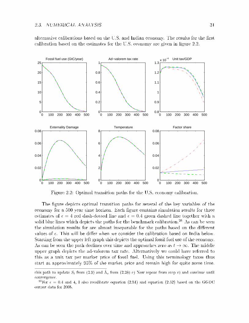
2.3. NUMERICAL ANALYSIS 31
alternative calibrations based on the U.S. and Indian economy. The results for the rstcalibration based on the estimates for the U.S. economy are given in gure 2.2.
0 100 200 300 400 5000
5
10
15
20
25Fossil fuel use (GtC/year)
0 100 200 300 400 5000
0.2
0.4
0.6
0.8
1Ad−valorem tax rate
0 100 200 300 400 5000.8
0.9
1
1.1
1.2
1.3x 10
−4 Unit tax/GDP
0 100 200 300 400 5000
0.02
0.04
0.06
0.08Externality Damage
0 100 200 300 400 5000
2
4
6
8Temperature
0 100 200 300 400 5000
0.02
0.04
0.06
0.08Factor share
Figure 2.2: Optimal transition paths for the U.S. economy calibration.
The gure depicts optimal transition paths for several of the key variables of theeconomy for a 500 year time horizon. Each gure contains simulation results for threeestimates of ε = 4 red dash-dotted line and ε = 0.4 green dashed line together with asolid blue lines which depicts the paths for the benchmark calibration.20 As can be seenthe simulation results for are almost inseparable for the paths based on the dierentvalues of ε. This will be dier when we consider the calibration based on India below.Starting from the upper left graph this depicts the optimal fossil fuel use of the economy.As can be seen the path declines over time and approaches zero as t→∞. The middleupper graph depicts the ad-valorem tax rate. Alternatively we could have referred tothis as a unit tax per market price of fossil fuel. Using this terminology taxes thusstart at approximately 95% of the market price and remain high for quite some time.
this path to update St from (2.9) and Λs from (2.28) e) Now repeat from step c) and continue untilconvergence.
20For ε = 0.4 and 4, I also recalibrate equation (2.51) and equation (2.52) based on the GGDCoutput data for 2005.

32 CHAPTER 2. STRUCTURAL AND CLIMATIC CHANGE
The upper left graph depicts the unit tax per unit of GDP. This graph is displayedin a scale that shows o the results for the dierent values of ε. As can be seen theupper line displaying the results for a ε = 0.4 implies a slightly higher tax for the entiretime period. Likewise, lower line displaying the results for a ε = 4 gives the lowesttax. The middle graph (blue line) depicts the benchmark case. Hence, we see that withincreasing values of ε the optimal tax rate declines. A carefull inspection of the optimalfossil fuel path graph also reveals that larger values of ε decreases the optimal fossilfuel use early on. Next the lower left graph displays the externality damage which isthe percent of damage to GDP as a function of tempertature increase. The lower linedisplays the amount of damage coming from the agricultural sector. Damages are lowerin this sector due to the fact that it constitutes a smaller proportion of GDP than themanufacturing sector. As can be seen for the manufacturing sector damages peaks atslightly above 6% of GDP after 200 years while the agricultural damages never goesabove 1% of GDP. The lower middle graph depicts the global temperature increases thatwould result following the emissions associated with the optimal path.21 Finally, thelower rightmost graph depicts the income factor shares corresponding to the expressionin proposition 2.1. As can be seen the diering values for ε creates clear trends when itcomes to the allocation of factor inputs. Here, the dash-dotted (red line) having an ε = 4creates a clear upward trend in factor input allocation implying that more resourcesare allocated to agriculture over time. This is due to the larger TFP estimate for theagricultural sector implying that the agricultural sector becomes more productive overtime. With an elasticity of substitution larger than one (i.e. substitutes) this impliesthat factor inputs are owing in to the more productive sector which can also be seenfrom the positive slope of the solid blue line. On the contrary the green dashed line isdownward sloping implying that resources are owing into the least productive sectoras it continues to grow relatively less productive.
Turn now to the Indian economy. Figure 2.3 displays the corresponding paths of forthe variables when the model has been calibrated to match the data from the Indianeconomy. As can be seen this gure displays a great deal more of variation in all of thedepicted variables. One major dierence between the Indian and U.S. calibrations wasthat the damage estimates for a 2.5 degree warming were substantially higher for theIndian economy. A comparison can be made in terms of ad-valorem taxes which forthe Indian economy constitutes approximately 100% of the market price at the outsetas opposed to 95% for the U.S. economy. This also results in a atter path of fossilfuel use since the higher damages makes it optimal to postpone fossil fuel consumptionto the future. As can be seen from the upper right graph the optimal paths vary agreat deal with the size of the elasticity of substitution. The red dash-dotted line withε = 4 the path exhibits a slight u-shape. Here damages early on are signicant enoughto warrant a lower level of fossil fuel use at the outset than after 200 years. From thelower right graph we see that this is likely to be connected to the increasing factor share
21These temperature levels are by many climate scienticts regarded as highly dangerous when itcomes to human survival on the planet (see e.g. Hansen (2005); Rockström et al. (2010)).

2.4. CONCLUDING REMARKS 33
0 100 200 300 400 5002
4
6
8
10
12Fossil fuel use (GtC/year)
0 100 200 300 400 5000
0.2
0.4
0.6
0.8
1Ad−valorem tax rate
0 100 200 300 400 5001.5
2
2.5
3
3.5x 10
−4 Unit tax/GDP
0 100 200 300 400 5000
0.05
0.1
0.15
0.2Externality Damage
0 100 200 300 400 5000
2
4
6
8Temperature
0 100 200 300 400 5000
0.5
1
1.5
2Factor shares
Figure 2.3: Optimal transition paths for the Indian economy calibration.
implying that resources are owing into the agricultural sector over time. Since thissector is less plagued with damages this explains why fossil fuel use starts to rise againafter approximately 100 years. The nal downturn after 250 years is of course due toresource scarcity leading to a rising relative price for fossil fuel consumption. From thelower lefthand graph depicting the externality damage as a percent of GDP we see thatdamages to the Indian economy are substantially higher than those observed for theU.S. economy peaking at roughly 15% of GDP after 300 years. From the temperaturegraph we see that this extra damage has however resulted in a more restrictive optimalfossil fuel use policy which keeps the global temperature from rising much higher than6 degrees as opposed to the near 7 degree peak in the U.S. economy.
2.4 Concluding remarks
In this paper I have developed a two-sector general equilibrium model featuring a globalclimate externality arising from the use of fossil fuels in production. I derive analyticaland numerical results for the optimal fossil fuel use in the social planner setting and thecorresponding unit and ad-valorem tax rates that implement the planner solution in adecentralized market equilibrium. I have shown that when the elasticity of substitutionbetween the two sectors is constant the same economic forces giving rise to structuralchange also impact the externality costs of climate change. The analytical results reveal

34 CHAPTER 2. STRUCTURAL AND CLIMATIC CHANGE
the behavior of optimal tax rates subject to sectoral dierences in damages, total factorproductivity and sectoral weights between the two sectors. It is shown that a higher(lower) elasticity of substitution will result in a higher (lower) optimal unit tax rate ifand only if the sectoral weight of the most productive sector, where productive refers tototal factor productivity net climate damages, is small (large) enough. The model andresults derived here draws upon the results and ndings of papers by Ngai and Pissarides(2007), Sterner and Persson (2008), Acemoglu and Guerrieri (2008) and Golosov et al.(2011).
Given a set of simplifying assumptions following Golosov et al. (2011) I am ableto derive i) a simple formula for the marginal externality cost of emissions and ii)a structural change mechanism which is almost identical to demand side mechanismdriving the results in Ngai and Pissarides (2007).22 However, in contrast to Ngai andPissarides (2007), the mechanism driving structural change in this paper is a combina-tion of damages and productivity assumptions which enter the model as a supply sidephenomena.
The numerical section of the paper gives a simulated example based on the U.S.and Indian economy. Calibrating the model to two economies at dierent stages ofdevelopment is a crude way of accommodating that systematic inter-sectoral dierencesin the elasticity of substitution, imply the possibility that the process of economicdevelopment itself might shift the over-all elasticity of substitution (Arrow et al., 1961).The results suggest that the elasticity of substitution plays a large role for optimalfossil fuel consumption in the Indian economy where the agricultural sector constitutesapproximately 20% of GDP. On the contrary the U.S. economy where the agriculturalsector constitutes only 1% of GDP this parameter plays only a peripheral role.
This paper has been a rst attempt at developing a climate-economy model where itis possible to explore how substitution possibilities among goods might impact growthand marginal externality costs. The model was developed in the tradition of modernmacroeconomic growth models with the intention of making it more accessible to em-pirical studies exploring the role of substitution possibilities for calculating the costsof climate change. A step for future research could be a more rigid calibration of themodel where for example the assumption of equal capital shares are also relaxed.
22If the climate externality is removed from the model developed here these mechanisms would havebeen identical.

References
Acemoglu D. and Guerrieri V., 2008, Capital Deepening and Nonbalanced Eco-nomic Growth, Journal of Political Economy, vol. 116(3).
Archer D., 2005, Fate of fossil fuel CO2 in geologic time, Journal of GeophysicalResearch, vol. 110(C9), pp. 16.
Arrow K.J., Chenery H.B., Minhas B.S. and Solow R.M., 1961, Capital-labor substitution and economic eciency, The Review of Economics and Statistics,vol. 43(3), pp. 225250.
Baumol W.J., 1967, Macroeconomics of Unbalanced Growth: The Anatomy of UrbanCrisis, American Economic Review, vol. LVII, pp. 415426.
Brock W.A. and Mirman L., 1972, Optimal Economic Growth and Uncertainty:The Discounted Case, Journal of Economic Theory, vol. 4(3), p. 479513.
Golosov M., Hassler J., Krusell P. and Aleh T., 2011, Optimal taxes on fossilfuel in general equilibrium, Working Paper 17348, National Bureau of EconomicResearch.
Hansen J.E., 2005, A slippery slope: How much global warming constitutes dangerousanthropogenic interference??, Climatic Change, vol. 68(3), pp. 269279.
Hassler J., Krusell P. and Olovsson C., 2011, Energy Saving Technical Change,mimeo, Institute of International Economic Studies, Stockholm University.
Hoel M. and Sterner T., 2007, Discounting and relative prices, Climatic Change,vol. 84(3-4), pp. 265280.
IPCC, 2001, Climate Change 2001: The Third Assessment Report of the Intergovern-mental Panel on Climate Change, Cambridge University Press, Cambridge.
IPCC, 2007, Climate Change 2007: The Fourth Assessment Report of the Intergovern-mental Panel on Climate Change, Cambridge University Press, Cambridge.
Irz X. and Roe T., 2005, Seeds of growth? Agricultural productivity and the transi-tional dynamics of the Ramsey model, European Review of Agricultural Economics,vol. 32(2), pp. 143165.
Knorr W., 2009, Is the airborne fraction of anthropogenic CO2 emissions increasing?,Geophysical Research Letters, vol. 36(L21710), pp. 15.
Lin J.Y. and Xu V.Z., 2011, The Hump-Shaped Structural Change, http://space.uibe.edu.cn/u1/venite/my%20web/hump-shaped.pdf.
35

36 CHAPTER 2. STRUCTURAL AND CLIMATIC CHANGE
Martin W. and Mitra D., 2001, Productivity Growth and Convergence in Agricul-ture versus Manufacturing, Economic Development and Cultural Change, vol. 49(2),pp. 403422.
Ngai L.R. and Pissarides C.A., 2007, Structural Change in a Multisector Model ofGrowth, American Economic Review, vol. 7(1), pp. 42943.
Nordhaus W. and Boyer J., 2000, Warming the World: Economic Models of GlobalWarming, MIT Press.
Nordhaus W.D., 1994, Managing the Global Commons: the economics of the green-house eect, MIT Press, Cambridge, MA.
Nordhaus W.D., 2007, A Question of Balance: Weighing the Options on GlobalWarming Policies, Tech. rep., Yale University.
Rockström J., Steffen W., Noone K., Persson A., Chapin F.S., LambinE.F., Lenton T., Scheffer M., Folke C., Schellnhuber H.J., NykvistB., Wit C.A.D., Hughes T., Leeuw S.V.D., Rodhe H., Sorlin S., Sny-der P.K., Costanza R., Svedin U., Falkenmark M., Karlberg L., CorellR.W., Fabry V.J., Hansen J., Walker B., Liverman D., Richardson K.,Crutzen P. and Foley J.A., 2010, A safe operating space for humanity, Nature,vol. 461(7263), pp. 472475.
Roe G.H. and Baker M.B., 2007, Why is climate sensitivity so unpredictable?, Sci-ence, p. 318: 629�632.
Rogner H.H., 1997, An Assessment of World Hydrocarbon Resources, Annual Reviewof Energy and the Environment, vol. 22, pp. 217262.
Ruttan V.W., 2002, Productivity Growth in World Agriculture: Sources and Con-straints, Journal of Economic Perspectives, vol. 16(4), pp. 161184.
Stanton E.A., Ackerman F. andKartha S., 2009, Inside the integrated assessmentmodels: Four issues in climate economics, Climate and Development, vol. 1, pp. 166184.
Sterner T. and Persson M., 2008, An Even Sterner Review: Introducing RelativePrices into the Discounting Debate, Review of Environmental Economics and Policy,vol. 2(1), pp. 6176.
Tans P., 2011, Trends in Carbon Dioxide, NOAA/ESRL, http://www.esrl.noaa.gov/gmd/ccgg/trends/index.html.
Timmer C.P., 2009, A World without Agriculture? The Historical Paradox of Agricul-tural Development, AEI Development Policy Outlook series. 1, American EnterpriseInstitute for Public Policy Research.

2.4. REFERENCES 37
Timmer M.P. and de Vries G.J., 2009, Structural Change and Growth Accelerationsin Asia and Latin America: A New Sectoral Data Set, Cliometrica, vol. 3(2), pp. 165190.
Tol R.S.J., 2009, The Economic Eects of Climate Change, Journal of EconomicPerspectives, vol. 23, pp. 2951.
Valentinyi A. and Herrendorf B., 2008, Measuring factor income shares at thesectoral level, Review of Economic Dynamics, vol. 11(4), pp. 820 835.
Weitzman M.L., 2010, What Is the "Damages Function" for Global Warming âand What Dierence Might It Make?, Climate Change Economics, vol. 01(01).

38 CHAPTER 2. STRUCTURAL AND CLIMATIC CHANGE
2.A Appendix
2.A.1 Static problem
Proof. of Proposition (2.1)Rewrite equation (2.12) as:
Kat
Kmt
=wawm
(YmtYat
) 1ε YatYmt
=
(wawm
YatYmt
) ε−1ε
LatLmt
=wawm
(YmtYat
) 1ε YatYmt
=
(wawm
YatYmt
) ε−1ε
EatEmt
=wawm
(YmtYat
) 1ε YatYmt
=
(wawm
YatYmt
) ε−1ε
(2.53)
where wa ≡ wε−1ε
a and wm ≡ wε−1ε
m . Further solving for the respective ratios we have
Kat
Kmt
=
((wawm
Ωa(St)
Ωm(St)
AatAmt
Lα2at
Lα2mt
Eα3at
Eα3mt
) ε−1ε
) εε−α1(ε−1)
LatLmt
=
((wawm
Ωa(St)
Ωm(St)
AatAmt
Kα1at
Kα1mt
Eα3at
Eα3mt
) ε−1ε
) εε−α2(ε−1)
EatEmt
=
((wawm
Ωa(St)
Ωm(St)
AatAmt
Kα1at
Kα1mt
Lα2at
Lα2mt
) ε−1ε
) εε−α3(ε−1)
denote ν1 ≡ ε−1ε−α1(ε−1)
, ν2 ≡ ε−1ε−α2(ε−1)
and ν3 ≡ ε−1ε−α3(ε−1)
.
Kat
Kmt
=
(wawm
Ωa(St)
Ωm(St)
AatAmt
) ε−1ε−α1(ε−1) Lat
Lmt
α2(ε−1)ε−α1(ε−1) Eat
Emt
α3(ε−1)ε−α1(ε−1)
(2.54)
LatLmt
=
(wawm
Ωa(St)
Ωm(St)
AatAmt
) ε−1ε−α2(ε−1) Kat
Kmt
α1(ε−1)ε−α2(ε−1) Eat
Emt
α3(ε−1)ε−α2(ε−1)
(2.55)
EatEmt
=
(wawm
Ωa(St)
Ωm(St)
AatAmt
) ε−1ε−α3(ε−1) Kat
Kmt
α1(ε−1)ε−α3(ε−1) Lat
Lmt
α2(ε−1)ε−α3(ε−1)
(2.56)
Substituting the labor share equation (2.55) into the capital share equation (2.54) andsolving for the capital share gives us
Kat
Kmt
=
(wawm
Ωa(St)
Ωm(St)
AatAmt
) ε−1ε−α1(ε−1)
(1+
α2(ε−1)ε−α2(ε−1)
)1−α1α2
ε−1ε−α1(ε−1)
ε−1ε−α2(ε−1) Eat
Emt
α3(ε−1)ε−α1(ε−1)
(1+
α2(ε−1)ε−α2(ε−1)
)1−α1α2
ε−1ε−α1(ε−1)
ε−1ε−α2(ε−1)
=
(wawm
Ωa(St)
Ωm(St)
AatAmt
) ε−1ε−α1(ε−1)−α2(ε−1) Eat
Emt
α3(ε−1)ε−α1(ε−1)−α2(ε−1)

2.A. APPENDIX 39
Now, substitute this into the labor share equation (2.55) to obtain
LatLmt
=
(wawm
Ωa(St)
Ωm(St)
AatAmt
Eα3at
Eα3mt
) ε−1ε−α2(ε−1)
+α1
ε−1ε−α1(ε−1)
ε−1ε−α2(ε−1)
(1+
α2(ε−1)ε−α2(ε−1)
)1−α1α2ν1ν2
=
(wawm
Ωa(St)
Ωm(St)
AatAmt
) ε−1ε−α1(ε−1)−α2(ε−1) Eat
Emt
α3(ε−1)ε−α1(ε−1)−α2(ε−1)
Substituting both these expressions into the emission share equation (2.56) we obtainafter som algebra
EatEmt
=
(wawm
Ωa(St)
Ωm(St)
AatAmt
) ε−1ε−(ε−1)(α1+α2+α3)
Further, from (2.53) we have that KatKmt
= LatLmt
= EatEmt
which implies that the solutionwill be equivalent for all factor inputs. Further it is clear that the above exponentssimplies to ε− 1 if we assume constant returns to scale.

40 CHAPTER 2. STRUCTURAL AND CLIMATIC CHANGE

Chapter 3
Energy Balance Climate Models and
General Equilibrium Optimal
Mitigation Policies∗
3.1 Introduction
The impact of climate change is expected to have a profound regional structure in termsof temperature and damage dierentials across geographical regions.1 The spatial di-mension of damages can be associated with two main factors: (i) Natural mechanismswhich produce a spatially non-uniform distribution of the surface temperature acrossthe globe. These mechanisms relate mainly to the heat ux that balances incomingand outgoing radiation and in the dierences among the local heat absorbing capacity- the local coalbedo - which is relatively lower in ice covered regions; (ii) economic re-lated forces which determine the damages that a regional (local) economy is expectedto suer from a given increase of the local temperature. These damages depend onpopulation size and production characteristics (e.g. agriculture vs services) or localnatural characteristics ( e.g. proximity and elevation from the sea level). The interac-tions between the spatially non-uniform temperature distribution and the spatially nonuniform economic characteristics will nally shape the spatial distribution of damages.
Existing literature and in particular the DICE/RICE models (e.g. Nordhaus andBoyer (2000), Nordhaus (2007, 2010, 2011)) provide a spatial distribution of damageswhere the relatively higher damages from climate change are concentrated to the zonesaround the equator.2 These models as well as the big majority of Integrated AssessmentModels (IAMs) do not account for the rst factor, the natural mechanism generating
∗This paper has been co-authored with William A. Brock and Anastasios Xepapadeas1Detailed reports of climate change eects on dierent parts of the world can be found at http:
//www.metoffice.gov.uk/climate-change/policy-relevant/obs-projections-impacts2For example, Nordhaus's RICE 2010 divides the world into US, EU, Japan, Russia, Eurasia,
China, India, Middle East, Africa, Latin America, Other high income, Other developing Asia. In theDICE model spatial damages are implicit in the aggregate representation since regional impacts areaggregated to a single measure using a bottom-up approach.
41

42 CHAPTER 3. EBCM'S AND THE CLIMATE-ECONOMY
temperature distribution across the globe. The DICE/RICE models do not includethe spatial transportation of heat, nor the albedo dierentials across locations, andperform their analysis in terms of the global mean surface temperature which does notvary across regions during their planning horizons.
In climate science terminology these IAMs can be referred to as zero-dimensionalmodels since they do not include spatial aspects such as heat diusion. This contrasts tothe one- or two-dimensional energy balance climate models (EBCMs) developed by cli-mate scientists which model heat diusion across latitudes (one-dimensional) or acrosslatitudes and longitudes (two-dimensional) ( see e.g. Budyko (1969), Sellers (1969,1976), North (1975a,b), North et al. (1981), Kim and North (1992), Wu and North(2007)). One-dimensional EBCMs predict a concave temperature distribution acrosslatitudes with the maximum temperature at the equator. This non uniform tempera-ture distribution is important for understanding the so called temperature anomalywhich is the dierence between the temperature distribution at a given benchmark pe-riod and the current period. Data indicate (Hansen et al., 2010) that since 1880 theanomaly has been relatively higher in high latitude zones, relative to zones around theequator, which suggest spatial non-uniformity in the distribution of temperature overtime.
The temperature anomaly is however the basis for estimating regional damages.Regional damages are obtained by mapping a given change in the temperature of aregion relative to a benchmark period (the temperature anomaly) to the damages thatthis change is expected to bring given the characteristics of the region's economy. Inthe context of a zero-dimensional model this temperature anomaly will be spatially ho-mogeneous, or at across regions, since climate change acts on the global average tem-perature which is spatially homogeneous. In the context of a one- or two-dimensionalmodel, climate change acts on the spatially non uniform temperature distribution. Thisis expected to result in a spatially non homogeneous distribution of the temperatureanomaly which in turn will dierentiate the distribution of damages from those impliedby a zero dimensional model.
In this paper we study the economics of climate change by coupling a one-dimensionalEBCM with heat diusion and albedo dierentiation across latitudes, with an economicgrowth model. We believe that this approach that integrates solution methods for one-dimensional spatial climate models, with methods of solving economic models, canprovide new insights regarding issues such as the prole of optimal mitigation policiesand the spatial distribution of damages, relative to the more conventional integratedassessment models with carbon cycle but without heat diusion. We focus on a popu-lar class of EBCMs, with analytical solutions derived in North (1975a,b); North et al.(1981)). These models feature (i) the explicit spatial dimension in the form of heatdiusion or transportion across latitudes using a heat diusion operator which allowsfor the use of approximation methods based on Legendre polynomial expansions, and(ii) the spatial dependency of earths albedo due to the presence of an endogenous iceline where latitudes north (south) of the ice line are solid ice and latitudes south (north)

3.1. INTRODUCTION 43
of the ice line are ice free.3
The economic part of the model is an innite horizon Ramsey-type model allowingfor basic heterogeneity among consumers and rms at each respective latitude denotedby "x". Considering each latitude as an individual economic zone is not the mostrealistic of assumptions but we believe this to be an important rst step before movingto more complex areas involving two-dimensional climate-economy models. Our basicanalytical approach is however very general and we need not conne x to meaning"latitude". At an analytical level of abstraction we just have to use a dierent basisset than Legendre polynomials.4 Hence, the results derived analytical in terms of e.g.optimal tax rates still hold with more complex diusion processes although numericalcomputations would have been more costly. The approach taken here and the resultsderived should thus be seen as an attempt to lay down a basic groundwork for futurestudies involving more complex interaction among economic zones and temperatureslocated on the sphere where x instead is interpreted as a "location" dened by both alatitude and a longitude.
Thus, in the context described above the main contribution of our paper is the cou-pling of a spatial climate model, implied by climate science, with a standard economicgrowth model. This allows us to explore what insights can be gained from the use ofeconomic-EBCMs when analyzing the temporal and spatial allocation decisions associ-ated with the climate change mitigation problem. Since EBCMs most likely are new tomost economist we have chosen to focus on the basic general equilibrium properties ofthe derived model under dierent assumptions regarding international capital marketsand their integration. This approach shows of the basic welfare properties of the modeland how the fundamental theorems of welfare economics apply within the context of ourenergy balance climate economy model. The approach also makes clear how the opti-mal carbon tax rates should be chosen in order to implement a social planning problemand should thus constitute an important rst step for economists working with thesetypes of models. We have chosen to look at three dierent cases here. The rst twocases concern economies that are either completely open or completely closed at eachrespective latitude. In the rst case when all economies are open capital returns andinterest rates will be equal across latitudes. In this case we show that the optimal car-bon tax will be uniform or equal across latitudes. In the second case when the economyis closed, interest rates and tax rates will generally dier across latitudes. In this caseif some countries are rich and some poor and international transfers are assumed to berestricted across latitudes, this will in general imply that optimal carbon taxes will be
3We could of course had considered other approaches alternative to EBCMs for approximatingtemperature elds which are based on more complex and computationally costly models, such aspattern scaling (Lopez et al., 2012) or emulation theory (Challenor et al., 2006). Because the purposeof this paper is however to construct the simplest coupled climate economy model with a climatefeedback response mechanism in space that responds to changes in the spatiotemporal structure oftaxes on fossil fuels, which is still analytically tractable, we considered the EBMCs framework as moreappropriate.
4For example, Wu and North (2007) show how similar approximation methods can be used in atwo-dimensional model featuring a "Fickian" diusion process across both latitudes and longitudes.
44 CHAPTER 3. EBCM'S AND THE CLIMATE-ECONOMY
spatially dierentiated. This result that in the absence of international transfers a spa-tially uniform optimal tax rate is in general not possible was rst noted by Chichilniskyand Heal (1994). Our result provides new insights into this issue by characterizing thespatial distribution of fossil fuel taxes and linking the degree of spatial dierentiationof optimal fossil fuel taxes to the diusion of heat across latitudes. The third andintermediate case we consider, extends our results beyond what was considered in thestatic model of Chichilnisky and Heal (1994). This concerns the case of costly transfersi.e. an open economy where transfers are available but come at a cost. In this case weshow that under the assumption that the marginal costs of international transfers doesnot change over time we can have both a spatially dierentiated tax rate and equalityamong interest rates across latitudes. Using these three separate scenarios we are ableto show how heat transport across latitudes matters regarding the prediction of thespatial distribution and the corresponding temporal evolution of temperature, damagesand optimal mitigation eorts. Our one-dimensional model further allows us to showhow heat diusion across geographical zones impacts on the size of the spatial dieren-tiation of fossil fuel taxes between poor and wealthy regions. In the numerical sectionof the paper we nally attempt a tentative calibration exercise and show how the openeconomy model can be solved numerically in order to obtain graphical representationsof e.g. damage and temperature distributions.
To sum up, the main objective of this paper has been to introduce the economicsprofession to spatial EBCMs with heat transport as a potentially useful tool for studyingthe economics of climate change relative to alternative zero dimensional models. Byderiving the spatiotemporal prole for optimal taxes from the one-dimensional coupledclimate economic model, we show how the spatial EBCMs can contribute to the currentdebate regarding how much to mitigate now, whether mitigation policies should bespatially homogeneous or not, and how to derive geographically specic informationregarding damages and policy measures.5
5Another issue that can be addressed by latitude dependent climate models is damage reservoirs.Damage reservoirs in the contest of climate change can be regarded as sources of climate damageswhich will eventually cease to exit when the source of the damages is depleted. Damage reservoirs arelatitude dependent and ice lines and permafrost can be regarded as such reservoirs.As the ice lines move closer to the poles, due to climate change, we might expect that marginal
damages from this moving will be large at rst and then diminish as the ice line approaches the Poles.When there will be no ice left on the Poles this damage reservoir would have been exhausted. Thepresence of an endogenous ice line in the EBCM allows us to model these type of damages explicitlygiven the relevant informationPermafrost is soil at or below the freezing point of water for two or more years. The permafrost
feedback suggests that permafrost carbon emissions could aect long-term projections of future tem-perature change. Studies indicate that up to 22 % of permafrost could be thawed already by 2100.Once unlocked under strong warming, thawing and decomposition of permafrost can release amountsof carbon until 2300 comparable to the historical anthropogenic emissions up to 2000 (approximately440 GTC) (Schneider et al., 2011).The modeling of damage reservoirs is beyond the scope of the present paper but we have addressed
this with in the context of a one-dimensional in a separate paper of ours (see Brock et al. (2012a)).Our ndings are that the introduction of damage reservoirs into the climate-economy framework may

3.2. AN ENERGY BALANCE CLIMATE MODEL WITH HUMAN INPUTS 45
Since these models are new in economics we proceed in steps that we believe makethis methodology accessible to economists.6 In section 3.2 we present a basic energybalance climate model which incorporates human impacts on climate which result fromcarbon dioxide accumulation due to the use of fossil fuels, that blocks outgoing ra-diation. In developing the model we follow North (1975a,b) and use his notation.We use the model to expose solution methods and especially the two mode approachwhich transforms systems of partial dierential equations (PDEs) in innite dimensionalspaces resulting from spatial modeling, into systems of ordinary dierential equations(ODEs) in nite dimensional spaces. The two mode approach will be used to solve, andnumerically approximate latitude dependent temperature and damage functions.
Section 3.3 couples the spatial EBCM with an economic growth model, where anite stock of fossil fuel is an essential input along with capital and labor. Fossil fuelsare extracted by fossil fuel rms which pay taxes on prots and/or taxes per unit offossil fuel extracted. We solve the model for the social planner and for the competitiveequilibrium with taxes. We derive the optimal taxes and their temporal proles. Weshow that under a mild assumption about a slow decay of the CO2 in the atmospherethe prot tax on fossil fuel rms decline over time and the unit taxes on extracted fossilfuels grow at rate less than the rate of return on capital. Furthermore we derive thelatitude dependent temperature function and the impact of heat transport on damagesacross latitudes.
In section 3.4 we use approximate solutions, we simulate the climate open economymodel and we derive explicit numerical solutions for the latitude dependent temporaland damage functions. The last section concludes.
3.2 An Energy Balance Climate Model with Human Inputs
In this section we develop a one-dimensional Energy Balance Climate Models with ahuman input. The addition of a human input will form the connection to the economicmodel developed in the following sections. The term one-dimensional means thatthere is an explicit spatial dimension in the model so that our unied model of theclimate and the economy evolves both in time and space.7 We follow North (1975a,b)and North et al. (1981) in this development. North developed his model in continuoustime. Here we work out the corresponding model in discrete time. The discrete timeframework oers a great deal of tractability given a specic set of assumptions notequally applicable in a continuous time framework. This will become clear when we
give rise to multiple steady states and Skiba points which can generate u-shaped optimal mitigationpolicies. Hence, we believe this represents an important area for further research.
6For more on EBCMs see for example Pierrehumbert (2008) (chapters 3 and 9, especially sections9.2.5 and 9.2.6 and surrounding material). North et al. (1981) is a very informative review of EBCMswhile Wu and North (2007) is a recent paper on EBCMs.
7In contrast, a zero-dimensional model does not explicitly account for the spatial dimension. Onthe other hand more complicated spatial structures could include two-dimensional spherical models.Our methods can be readily extended to a two dimensional spherical model as in Wu and North (2007).

46 CHAPTER 3. EBCM'S AND THE CLIMATE-ECONOMY
couple the model to the economic growth model in the following section.8
Let x to denote the sine of the latitude. We shall abuse language and just refer to xas latitude. Following North (1975a,b) let Ix,t denote outgoing infrared radiation uxmeasured in W/m2 at latitude x at time t, Tx,t denote surface (sea level) temperaturemeasured in C at latitude x at time t. The outgoing radiation and surface temperaturecan be related through the empirical formula.9
Ix,t = A+BTx,t (3.1)
The basic energy balance equation developed in (North (1975a), equation (29)) can bewritten, with human input added hx,t, as:
c(Ix,t+1 − Ix,t) = QS(x)α(x, xs,t)− [Ix,t − hx,t] +D∂
∂x
[(1− x2)
∂Ix,t∂x
](3.2)
where units of x are chosen so that x = 0 denotes the Equator, x = 1 denotes the NorthPole, and x = −1 denotes the South Pole; Q is the solar constant divided by 4;10 S(x)is the mean annual meridional distribution of solar radiation which is normalized sothat its integral from -1 to 1 is unity; α(x, xst) is the absorption coecient or co-albedofunction which is one minus the albedo of the earth-atmosphere system, with xst beingthe latitude of the ice line at time t; and D is a thermal diusion coecient. Followinglater work by North et al. (1983) c can be interpreted as an absorption factor. Moreabout this below.
Equation (3.2) states that the rate of change of outgoing radiation is determinedby the dierence between the incoming absorbed radiant heat QS(x)α(x, xst) and theoutgoing radiation [Ix,t − hx,t] . Note that the outgoing radiation is reduced by thehuman input hx,t. We associate human input with injection of carbon dioxide into theatmosphere at latitude x. We will throughout this paper assume that emissions ofcarbon dioxide from human activities at latitude x disperses rapidly across latitudes sothat hx,t = hx′,t, ∀x, t. This implies that we can replace hx,t in (3.2) with ht, whichwill represent the aggregate human forcing on the climate system coming from theaccumulation of carbon dioxide in the atmosphere dened as ht ≡
∫ 1
−1hx,tdx.
We approximate human related forcing based on table 6.2 of the IPCC (2001) report.Dene human related forcing as ht = ξ ln
(1 + Mt
M
)where M denotes the pre-industrial
atmospheric CO2 concentration and Mt stock of carbon dioxide in the atmosphere attime t above pre-industrial levels, where ξ denotes the approximate radiative forcing(W/m2).
8For a continuous time analog of our derivations in this section see Brock et al. (2012b).9It is important to note that the original Budyko (1969) formulation cited by North parameterizes
A,B as functions of fraction cloud cover and other parameters of the climate system. North (1975b)points out that due to non-homogeneous cloudiness A and B should be functions of x. There isapparently a lot of uncertainty involving the impact of cloud dynamics (e.g. Trenberth et al. (2010)versus Lindzen and Choi (2009)). Hence robust control in which A,B are treated as uncertain may becalled for but this is left for further research.
10The solar constant includes all types of solar radiation, not just the visible light. It has beenmeasured by satellite to be roughly 1.376 kilowatts per square meter (kW/m2) North et al. (1981).

3.2. EBCM WITH HUMAN INPUTS 47
The stock of the atmospheric carbon dioxide evolves according to
Mt+1 −Mt = σ
∫ x=1
x=−1
qx,tdx−mMt, M0 = M00 (3.3)
where σqx,t are emissions generated at latitude x, with emissions being proportionalto the amount of fossil fuels used by latitude x at time t. The coecient σ reectsemission intensity of the fossil fuels and m is the carbon dioxide removal rate from theatmosphere.
We assume that the total stock of fossil fuel available is xed or,∫ x=1
x=−1
qx,tdx = qt ,∞∑t=0
qt ≤ R0 (3.4)
where qt is total fossil fuels used across all latitudes at time t, and R0 is the totalavailable amount of fossil fuels on the planet. Thus in this model the use of fossil fuelsgenerates emissions, emissions increase the stock of atmospheric carbon dioxide, whichin turn increases the temperature by blocking the amount of outgoing "long-wave"radiation.
As pointed out by North (1975b), in equilibrium at a given latitude the incomingabsorbed radiant heat is not matched by the net outgoing radiation and the dier-ence is made by the meridional divergence of heat ux which is modeled by the termD ∂
∂x
[(1− x2)∂Ix,t
∂x
]. This term explicitly introduces the spatial dimension, stemming
from the heat transport, into the climate model.Returning to the description of (3.2), the ice line is determined dynamically by the
condition (Budyko, 1969; North, 1975a,b):
T > −10oCno ice line present at latitude xT < −10oC ice present at latitude x (3.5)
and `below' the ice line absorption drops discontinuously because the albedo jumpsdiscontinuously. For example North (1975a) species, discontinuous co-albedo functionas:
α(x, xs) =
α0 = 0.38 |x| > xsα1 = 0.68 |x| < xs
(3.6)
3.2.1 Approximating Solutions for the Basic Energy Balance
Equation
We turn now to a more detailed analysis of the solution process. Equation (3.2) is aPDE. One might think that we are going to have to deal with the complicated mathe-matical issues of the solution or the optimal control of PDEs when we need to discussthe economic optimization problems over space and time. But, as we shall see, theclimate problem reduces to the optimal control of a small number of modes whereeach mode follows a simple ODE. We believe this decomposition is another impor-tant and new contribution of our paper to the study to coupled economic and climate
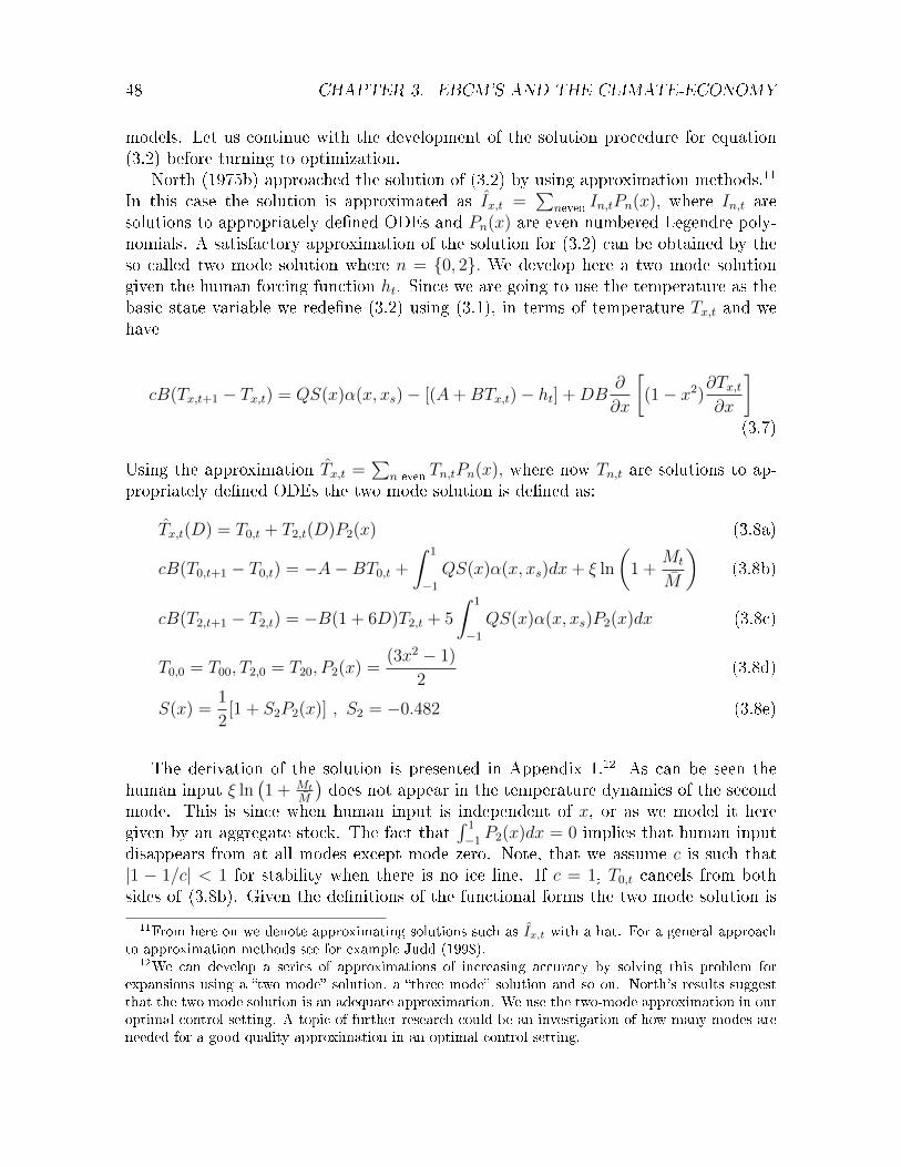
48 CHAPTER 3. EBCM'S AND THE CLIMATE-ECONOMY
models. Let us continue with the development of the solution procedure for equation(3.2) before turning to optimization.
North (1975b) approached the solution of (3.2) by using approximation methods.11
In this case the solution is approximated as Ix,t =∑
neven In,tPn(x), where In,t aresolutions to appropriately dened ODEs and Pn(x) are even numbered Legendre poly-nomials. A satisfactory approximation of the solution for (3.2) can be obtained by theso called two mode solution where n = 0, 2. We develop here a two mode solutiongiven the human forcing function ht. Since we are going to use the temperature as thebasic state variable we redene (3.2) using (3.1), in terms of temperature Tx,t and wehave
cB(Tx,t+1 − Tx,t) = QS(x)α(x, xs)− [(A+BTx,t)− ht] +DB∂
∂x
[(1− x2)
∂Tx,t∂x
](3.7)
Using the approximation Tx,t =∑
n evenTn,tPn(x), where now Tn,t are solutions to ap-
propriately dened ODEs the two mode solution is dened as:
Tx,t(D) = T0,t + T2,t(D)P2(x) (3.8a)
cB(T0,t+1 − T0,t) = −A−BT0,t +
∫ 1
−1
QS(x)α(x, xs)dx+ ξ ln
(1 +
Mt
M
)(3.8b)
cB(T2,t+1 − T2,t) = −B(1 + 6D)T2,t + 5
∫ 1
−1
QS(x)α(x, xs)P2(x)dx (3.8c)
T0,0 = T00, T2,0 = T20, P2(x) =(3x2 − 1)
2(3.8d)
S(x) =1
2[1 + S2P2(x)] , S2 = −0.482 (3.8e)
The derivation of the solution is presented in Appendix 1.12 As can be seen thehuman input ξ ln
(1 + Mt
M
)does not appear in the temperature dynamics of the second
mode. This is since when human input is independent of x, or as we model it heregiven by an aggregate stock. The fact that
∫ 1
−1P2(x)dx = 0 implies that human input
disappears from at all modes except mode zero. Note, that we assume c is such that|1 − 1/c| < 1 for stability when there is no ice line. If c = 1, T0,t cancels from bothsides of (3.8b). Given the denitions of the functional forms the two mode solution is
11From here on we denote approximating solutions such as Ix,t with a hat. For a general approachto approximation methods see for example Judd (1998).
12We can develop a series of approximations of increasing accuracy by solving this problem forexpansions using a two mode solution, a three mode solution and so on. North's results suggestthat the two mode solution is an adequate approximation. We use the two-mode approximation in ouroptimal control setting. A topic of further research could be an investigation of how many modes areneeded for a good quality approximation in an optimal control setting.

3.2. EBCM WITH HUMAN INPUTS 49
tractable and can be calculated given initial conditions T00, T02 which are determinedby the initial climate state.
In the two-mode solution, the ice line function xs(t) which determines the co-albedosolves the equation Is = I(xs(t), t). In terms of temperature and the using the two-modesolution, the ice line function solves
Tx,t(D) = T0,t + T2,t(D)P2(xst) = Ts, Ts = −10oC (3.9)
and the ice line function is given by a solution of (3.9), i.e.
xst = P−1+
(Ts − T0,t
T2,t(D)
)(3.10)
Where the subscript + denotes the largest inverse function of the quadratic func-tion P2(x) := (1/2)(3x2−1). Notice that the inverse function is unique and is the largestone on the set of latitudes [−1, 1]. Thus there exist a nonlinear feedback from changesin temperature to the co-albedo thought the endogeneity of the ice line. This feed-back can be simplied by making the co-albedo function α(x, xs) a smooth function ofthe temperature, α(x, Tx,t(D)) which can be highly nonlinear around −10oC.13 A moresimplied and tractable specication of the co-albedo is the one introduced by Northet al. (1981) (p.95 equation (18)), where the co-albedo depends only on geographicallocation or
a(x) = 0.681− 0.202P2(x) (3.11)
In this case the co-albedo function retains its latitude dependence and provides asignicant simplication that helps tractability.
Use of global mean temperature and potential bias
The two-mode solution denes the climate module by (3.8a)-(3.8e), and (3.3),(3.4).Although the climate module does not contain the PDE (3.7) that incorporates tem-perature diusion, spatial interactions are incorporated through the mode-2 part ofthe solution the ODE (3.8c). Thus the contribution of the second mode into the fullsolution can be regarded as the importance of space through heat transport, in theanalysis of climate change. This can be seen by the following argument.
The size of diusion coecient D determines the speed of spatial diusion in (3.7).If D = 0 then are no spatial interactions, if D →∞ then we have instantaneous mixingand spatial homogeneity and thus the heat transport across latitudes is not relevant forour problem. In this case, the mode two solution vanishes. To show this note that sincethe total amount of fossil fuel is nite and the contributions to the stock of atmosphericcarbon dioxide is due to the use of fossil fuels, the stock of the atmospheric carbondioxide M (t) must be bounded above. Thus the second term of the right hand side of(3.8c) is bounded above. Then the following proposition can be stated
13For example the co-albedo function α (x, T (x, t)) = c0 + c1 tanh (T (x, t) + 10) for (c0, c1) =(.525, .195) provides a good approximation of the discontinuous function dened by (3.5)-(3.6).

50 CHAPTER 3. EBCM'S AND THE CLIMATE-ECONOMY
Proposition 3.1. Assume that∫ 1
−1QS(x)α(x, xs)P2(x)dx ≤ UB <∞, and that D →
∞. Then the solution T2,t of (3.8c) vanishes.
Proof. equation (3.8c) can be written asc(T2,t+1 − T2,t) = −(1 + 6D)T2,t + (5/B)
∫ 1
−1QS(x)α(x, xs)P2(x)dx. As D → ∞ any
steady state of (3.8c) dened as T+2,t = 5
B(1+6D)
∫ 1
−1QS(x)α(x, xs)P2(x)dx→ 0. Further-
more, consider the ODE
c(T2,t+1 − T2,t) = −(1 + 6D)T2,t + (5/B)UB. (3.12)
Since c(T2,t+1 − T2,t) ≤ −(1 + 6D)T2 + (5/B)UB, then by Gronwall's inequality thesolution of (3.8c) will be bounded above by the solution T2,t of (3.12). This solutionhowever goes to zero as D →∞. Therefore T2,t → 0 as D →∞.
Thus for a given diusion D < ∞ the relative contribution of T2,t to the solutionTx,t can be regraded as an a measure of whether the heat transport is important in thesolution of the problem.
This result can be used to suggest that the use of the global mean temperature alonein IAMs may introduce a bias. From the two mode approximation of the temperature,we obtain the global mean temperature as mT = T0,t.
14 This result, along with proposi-tion 1, indicates that the zero - dimensional IAMs can be regarded as a special case of aone-dimensional model when D →∞. Thus the second mode that provides that spatialdistribution of temperature is omitted in the zero - dimensional IAMs. Since scienticevidence indicate that D is small (less than one according to North et al. (1981)) ourresult suggest that the dropping of the second mode by the IAMs introduces a kind ofbias. In our paper we correct for this underlying bias by keeping that second mode,and we also provide a basis for a quantitative representation of this bias. The varianceof the global mean temperature is:
VT =
∫ 1
−1
[Tx,t(D)− T0,t
]2
dx =
∫ 1
−1
(T2,t(D)P2(x))2dx =2
5(T2,t(D))2 (3.13)
In an IAM this variance will be zero since the second mode is dropped.Local temperature means at latitudes (x, x+dx) and the mean of temperature over
the set of latitudes Z = [a, b] are dened by
[T0,t + T2,t(D)P2(x)] dx, m [a, b] =
∫ b
a
[T0,t + T2,t(D)P2(x)] dx (3.14)
while the variance of temperature over the set of latitudes Z = [a, b] is
V [a, b] =
∫ b
a
[T0,t + T2,t(D)P2(x)−m [a, b; t]]2 dx (3.15)
14This is because mT =∫ 1
−1 Tx,tdx =∫ 1
−1 [T0,t + T2,tP2(x)] dx and∫ 1
−1 P2(x)dx = 0.

3.3. AN ECONOMIC EBC MODEL 51
It might be plausible to assume that utility in each area [a, b] depends upon both themean temperature and the variance of temperature in that area. For example we mayexpect increases in mean temperature and variance to have negative impacts on outputin any area Z, if it is located in tropical latitudes. Whereas mean temperature increasesin some areas Z (e.g. Siberia) may increase utility rather than decrease utility.15
3.3 An Economic EBC Model
In this section we characterize the solution to the planning problem. Based on theresults of section 3.2 this implies that a well dened planning problem should considerresource allocation across both time and space. For the remainder of the paper wedrop the hat (Tx,t) notation for local temperature to ease up on notation. If nothingelse is stated Tx,t henceforth refers to the approximate solution given by (3.8). We rstdescribe the general features of the economy and then proceed with the problem of theplanner. In the proceeding section we then characterize the market equilibrium.
3.3.1 General features of the economy
The economy is assumed to be inhabited by a representative household at latitude xhaving preferences dened by the following utility function.16
U(Cx,t/Lx,t) =(Cx,t/Lx,t)
1−θ − 1
(1− θ)(3.16)
where Cx,t denotes aggregate consumption and Lx,t the size of the representative house-hold (equal to population) at time t and for latitude x. U is thus a standard concaveutility function having a constant inter-temporal elasticity of substitution 1/θ. Laboris supplied inelastically and is equal to population, which grows at a constant factor nso that Lx,t = Lx,0n
t−1. Production takes place separately at each latitude
Yx,t = Ax,tΩ(Tx,t)F (Kx,t, Lx,t, qx,t) (3.17)
where Kx,t, Lx,t, qx,t denote capital, labor and fossil fuels respectively used at latitudex, and time t, a is the TFP growth so that Ax,t = Ax,0a
t−1, and Ω(Tx,t) are the damagesto output due to climate change occurring at latitude x and time t as a function of the
15In a stochastic generalization of our model, we could introduce a stochastic process to representweather, i.e. very high frequency uctuations relative to the time scales we are modeling here.Here the local variance of high frequency phenomena like weather may change with changes inlower frequency phenomena such as mean area Z temperature and area Z temperature variance. Weleave this task to future research. Existing dynamic integrated models of climate and economy, (e.g.Nordhaus's well known work (2007, 2010)) can not deal with these kinds of spatial elements, such asimpacts of changes in temperature variance, generated by climate dynamics over an area Z.
16We will throughout the rest of the paper think of x as being a country when discussing economicactivity along a specic latitude. This is of course a ludicrous abstraction from reality. However, asthis paper constitutes a rst stab at bringing in latitude dependent temperatures into climate-economymodels we have preferred to stick to a general setting, prioritizing mathematical neatness and thusleaving more realistic descriptions for future research.

52 CHAPTER 3. EBCM'S AND THE CLIMATE-ECONOMY
local temperature at the that latitude, with ∂Ω(Tx,t)
∂Tx,t< 0. The total amount of fossil fuels
available is nite and given by equation (3.4) of the previous section. The spatial aspectof our model also induces the possibility to consider the possibility of intertemporaltrade. We denote the net stock of foreign bond or asset holdings at latitude x byBx,t which generate a return Rt. Negative values thus implies that latitude x has anoutstanding debt to other latitudes. The budget constraint of each country is thusgiven by
Cx,t +Kx,t+1 +Bx,t+1 ≤ Yx,t + (1− δ)Kx,t +RtBx,t (3.18)
from which we can write the global budget constraint by integrating over x
Ct +Kt+1 ≤ Yt + (1− δ)Kt (3.19)
where17
0 =
∫x
Bx,tdx, Ct =
∫x
Cx,tdx, Kt =
∫x
Kx,tdx, Yt =
∫x
Yx,tdx (3.20)
3.3.2 Global welfare maximization
Given the description of the economy and climate dynamics provided so far, it is clearthat the welfare maximization problem of a planner, should involve both spatial andintertemporal decision making. We formalize this by dening a global social welfarefunction where each individual country is pre-assigned a specic welfare weight, so thatby varying these weights we can trace out dierent distributional outcomes for theglobal economy. The welfare function of the planner can be written as
∞∑t=0
βt∫x
υ (x)Lx,tU(Cx,t/Lx,t)dxdt (3.21)
where β represents the discount factor and υ(x) denotes the latitude specic welfareweight assigned to the planner.18 An early result noted by Chichilnisky and Heal (1994)shows that in a multi-country optimal planning problem featuring both a private and apublic good, whether the solution to the problem will equalize marginal abatement costsacross countries will largely depend upon whether international transfers are availableor not.19 In the absence of such transfers a spatially uniform carbon tax is thus ingeneral not possible.20 Within the one-dimensional energy balance model we consider
17To ease notation we introduce the∫xwhich denotes the integral over all x's and is equivalent to∫ 1
−1 used previously. We will use these interchangeably from here on.18The welfare weights are assigned so that
∫xυ(x)dx = 1. An example of a weight independent of x
would be υ(x) = 1/2.19Similar results have also been obtained by (Chichilnisky et al., 2000; Shiell, 2003b; Sandmo, 2006;
Antho, 2011; Keen and Kotsogiannis, 2011).20Transfers of this kind are signicant and observed in the real world not only in terms of foreign
aid and development assistance but also in terms of payments for the supply of public goods examplesinclude the Joint implementation and Clean development mechanisms incorporated into the Kyotoprotocol. However, it is also true that countries to a great extent are limited by their own resourcesand incomes.
3.3. AN ECONOMIC EBC MODEL 53
here, the heat diusion across latitudes creates a spatially dierentiated damage func-tion which makes the results of Chichilnisky and Heal (1994) increasingly relevant. Inparticular, since international transfers may many times prove to be hard to implementin practice.21 In order to highlight the role of international transfers we will considerthree specic cases.
In the rst case, which we will refer to as the open economy problem, the economy iscompletely open with free ows of capital, fossil fuel and consumption goods across lat-itudes. This implies that returns to capitals and bonds will be equal across latitudes.22
The planner has the power to administer lump-sum transfers of goods across latitudeswhich implies that all Pareto optimal allocations corresponding to a particular set ofwelfare weights can be traced out. Due to his ability to freely transfer goods acrosslatitudes the investment decisions of this planner is thus not limited by the capitalbudget constraint (3.18) involving each individual latitude but rather the sum, or aswe have chosen to model it here, the integral over all latitude specic capital budgetconstraints.
Turning to the second case. We refer to this case as the closed economy problemsince each latitude is limited by its own budget constraint. As will be shown, in thiscase, depending on whether the planner has access to international transfers or not,optimal tax rates may dier across latitudes. The particular assumptions connectedto this scenario are restrictive and perhaps not so realistic but they help bring out theforces that can generate spatially dierentiated taxe rates. In particular we show thatif wealth transfers are restricted and welfare weights are assumed to be equal acrosslatitudes this implies that optimal tax rates will be spatially dierentiated.
Finally the last case we consider concerns when transfers are costly. In this caseinternational transfers are possible but no longer free. This case constitutes a middleway between the closed economy and open economy case. Here we show that as withthe case of the closed economy, the tax or social price connected to the use of fossilfuels may dier across latitudes.
We start by solving the open economy problem involving free international trans-fers. We then characterize the competitive equilibrium and derive the optimal tax rateswhich implement the planning solution. In the following sections we will explore thealternative representations. For all these cases we will employ the two mode approx-imation dened in section 3.2 when introducing the economic model to the climatedynamics of EBCM's.
21Shiell (2003a) points to e.g. to corruption as one possibility that can make large internationaltransfers unfeasible. In this case, the opportunity to help the poor through untied transfers may beseriously compromised by misappropriation or theft by ocials who are charged with administeringthe transfers in recipient countries.
22We neglect migration and assume labor is completely immobile across latitudes. Labor immobilityat a global scale could be regarded as a reasonable approximation given restrictions on labor mobilityrelative to capital and fossil fuel mobility.

54 CHAPTER 3. EBCM'S AND THE CLIMATE-ECONOMY
3.3.3 Optimal planning problem with open markets and free
international transfers
Given the economy and climate dynamics described above we start by considering thewelfare maximization problem of an open economy where the planner has free access tointernational transfers across latitudes. In this case the planner maximizes the welfarefunction dened in equation (3.21) subject to (3.3),(3.4), (3.8), (3.19) and (3.20). Ascan be seen from inspection of this maximization problem, it can be broken downinto a static and dynamic problem which can be considered separately. We start bycharacterizing the static problem.
Static problem
The spatial allocation decision facing the planner involves the allocation of consumption,capital and fossil fuels to each latitude so as to maximize global output and social welfarein each time period subject to the global capital budget constraint (3.19). As will beseen the solution to this problem implies that the marginal products of Kx,t and qx,tmust be equal across latitudes and that the weighted marginal utility of Cx,t at eachlatitude must also be equal.
First, in order to determine how capital and fossil fuels are allocated across latitudesgiven the global intertemporal investment and fossil fuel use decisions governed by thecapital budget constraint, we proceed by solving the following problem; assuming aCobb-Douglas production function:23
Ftotal(Kt, qt, Tx,tx=1x=−1 ; t) ≡ max
∫x
(anαL)t−1Ax,0LαLx,0Ω(Tx,t)K
αKx,t q
αqx,tdx
= (anαL)t−1KαKt q
αqt max
∫x
Ax,0LαLx,0Ω(Tx,t)(Kx,t/Kt)
αK (qx,t/qt)αqdx
s.t.∫x
Kx,t/Ktdx ≤ 1,
∫x
qx,t/qtdx ≤ 1 (3.22)
We dene Ftotal(Kt, qt, Tx,tx=1x=−1 ; t) as the potential world GDP at date t. This con-
cept represents the maximum output that the whole world can produce given to-tal world capital Kt available and total world fossil fuel qt used, for a given distri-bution of temperature Tx,t across the globe, with labor growing with the constantfactor n, and treated as immobile. Thus Ftotal can be regarded as a natural baseline under ideal world conditions where there's no barriers to capital and fossil fuelows to their most productive uses across latitudes.24 We abuse notation and writeFtotal(Kt, qt, Tx,tx=1
x=−1 ;x, t) = Ftotal(Kt, qt, T ; t). Next, dene the shares of K and q at
23Hassler et al. (2011) argue that, on shorter time horizons, Cobb-Douglas production does notrepresent a good way of modeling energy demand since it does not capture the joint shorter- to medium-run movements of input prices and input shares. However, On longer time horizons considered here itis more reasonable since input shares do not appear to trend.
24This notion can be regarded as similar to the notions of potential GDP potential output etcused by macro economists.

3.3. AN ECONOMIC EBC MODEL 55
date t by SKx,t ≡ Kx,t/Kt and Sqx,t ≡ qx,t/qt. It is now easy to check that the optimal
shares solving problem (3.22) will be given by25
SKx,t = Sqx,t = (Ax,0LαLx,0Ω(Tx,t))
1αL /
∫x
(Ax,0LαLx,0Ω(Tx,t))
1αL dx (3.23)
Substituting the optimal shares back into the objective function we obtain the followingexpression for potential world GDP
Ftotal(Kt, qt, Tx,tx=1x=−1 ; t) = (anαL)t−1KαK
t qαqt
(∫x
(Ax,0LαLx,0Ω(Tx,t))
1αL dx
)αL(3.24)
As it can be seen from (3.24) the Cobb-Douglas specication allows the separation ofthe climate damage eects on production across latitudes. Dene
J(Tx,tx=1
x=−1
)≡(∫
x
(Ax,0LαLx,0Ω(Tx,t))
1αL dx
)αL(3.25)
This expression depends on the thermal diusion coecient D which multiplies a pro-duction function that is independent of x. Thus population growth and technical changeaect the macrogrowth component (anαL)t−1KαK
t qαqt , while changes in the size of D
have a direct eect on the climate component. The combination of the macrogrowthand the climate component determine the potential world input.
Second, the allocation consumption across latitudes is solved in an equivalent man-ner by maximizing (3.21) subject to
∫x′Cx′,t ≤ Ct. Hence, Cx,t is restricted by the total
amount of available consumption Ct which in turn is restricted by the global capitalbudget constraint. The rst order conditions with respect Cx,t thus implies
v(x)βtU ′(Cx,t/Lx,t) = v(x′)βtU ′(Cx′,t/Lx′,t) (3.26)
which further implies that
Ct =
∫x′Cx′,tdx
′ =
∫x′
(v(x)
v(x′)
Lθx,tLθx′,t
)−1θ
Cx,tdx′
= (v(x)Lθx,0)−1θ
∫x′
(v(x′)Lθx′,0
) 1θ dx′Cx,t (3.27)
as with the capital and fossil fuel shares we dene consumption shares as SCx,t ≡ Cx,t/Ct.
The dynamic problem
Together the static solutions (3.24) and (3.27) allows us to write the ideal planningproblem completly in aggregate terms. Integrating (3.18) over x after having substitutedin the static solutions we can thus express the ideal planning problem as
max∞∑t=0
(βnθ)tU(Ct), (3.28)
s.t. Ct +Kt+1 ≤ Yt + (1− δ)Kt (3.29)
25See appendix for a complete derivation.

56 CHAPTER 3. EBCM'S AND THE CLIMATE-ECONOMY
and (3.3),(3.4),(3.8) where Yt ≡ Ftotal(Kt, qt, T ; t). The rst order necessary conditionsw.r.t. Kt+1 gives us the standard Euler equation
U ′(Ct) = βnθU ′(Ct+1)
(∂Yt+1
∂Kt+1
+ (1− δ)
)(3.30)
Since the problem is concave in K this is sucient for optimum over K. Turn nowto optimization w.r.t. q. At each date t a small increase in qt gets a marginal gain inoutput at t but sets of a sequence of marginal changes in damages for periods t+1, t+2, .The rst order necessary conditions for qt at date t is given by
(βnθ)tU ′(Ct)∂Yt∂qt
= −∞∑k=2
(βnθ)t+kU ′(Ct+k)∂Yt+k∂Tx,t+k
∂Tx,t+k∂Mt+k−1
∂Mt+k−1
∂qt+ µ0 (3.31)
This expression is fundamental to our paper as it characterizes how the spatial aspectsaect optimal fossil fuel use.26 It is also straightforward to interpret. The rst ordercondition simply states that the marginal social utility of using an extra unit of fossil fuel(left hand side) must equal the marginal social cost (right hand side). The marginalsocial cost consists of both the capitalized sum of marginal damages to output att + 1, t + 2, ... plus the marginal cost of not having that unit of fossil fuel available inthe future (when R0 is ultimately all used up).27
Alternatively, the capitalized sum of marginal damages could have been expressedas in Golosov et al. (2011) in terms of a shadow price (λs)
λst ≡ −∞∑k=2
(βnθ)t+kU ′(Ct+k)∂Yt+k∂Tx,t+k
∂Tx,t+k∂Mt+k−1
∂Mt+k−1
∂qt(3.32)
or alternatively, in consumption units Λst ≡ λst/U
′(Ct)
Λst ≡ −
∞∑k=2
(βnθ)t+kU ′(Ct+k)
U ′(Ct)
∂Yt+k∂Tx,t+k
∂Tx,t+k∂Mt+k−1
∂Mt+k−1
∂qt(3.33)
Equation (3.33) is thus our analog of equation 11 in Golosov et al. (2011). We can nowfrom equation (3.31) write down a spatial version of the climate externality adjusted
26The formula was derived using c = 1 in (3.8). This simplies the f.o.c. which otherwise wouldhave been given by
(βnθ)tU ′(Ct)∂Yt∂qt
= −∞∑k=2
(βnθ)t+kU ′(Ct+k)∂Yt+k∂Tt+k
(k−1∑s=1
∂Tt+k∂Mt+s
∂Mt+s
∂qt
)+ µ0
We will keep this assumption throughout the rest of the paper.27When there are damages to consumption, there will be an extra term on the right hand side
representing the capitalized sum of marginal damages to future social utility of climate during thefollowing dates. This term can be potentially important for optimal mitigation decisions as shown inSterner and Persson (2008). For simplicity we abstract from this here.
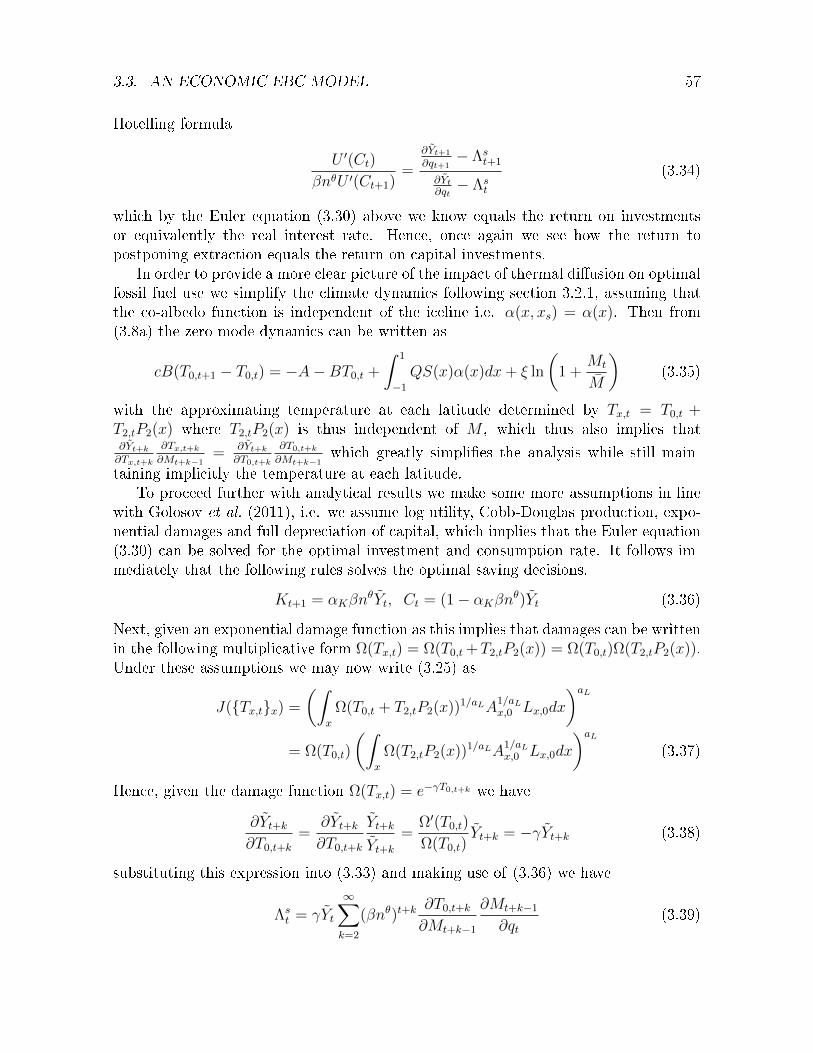
3.3. AN ECONOMIC EBC MODEL 57
Hotelling formula
U ′(Ct)
βnθU ′(Ct+1)=
∂Yt+1
∂qt+1− Λs
t+1
∂Yt∂qt− Λs
t
(3.34)
which by the Euler equation (3.30) above we know equals the return on investmentsor equivalently the real interest rate. Hence, once again we see how the return topostponing extraction equals the return on capital investments.
In order to provide a more clear picture of the impact of thermal diusion on optimalfossil fuel use we simplify the climate dynamics following section 3.2.1, assuming thatthe co-albedo function is independent of the iceline i.e. α(x, xs) = α(x). Then from(3.8a) the zero mode dynamics can be written as
cB(T0,t+1 − T0,t) = −A−BT0,t +
∫ 1
−1
QS(x)α(x)dx+ ξ ln
(1 +
Mt
M
)(3.35)
with the approximating temperature at each latitude determined by Tx,t = T0,t +T2,tP2(x) where T2,tP2(x) is thus independent of M , which thus also implies that∂Yt+k∂Tx,t+k
∂Tx,t+k∂Mt+k−1
= ∂Yt+k∂T0,t+k
∂T0,t+k∂Mt+k−1
which greatly simplies the analysis while still main-taining implicitly the temperature at each latitude.
To proceed further with analytical results we make some more assumptions in linewith Golosov et al. (2011), i.e. we assume log utility, Cobb-Douglas production, expo-nential damages and full depreciation of capital, which implies that the Euler equation(3.30) can be solved for the optimal investment and consumption rate. It follows im-mediately that the following rules solves the optimal saving decisions.
Kt+1 = αKβnθYt, Ct = (1− αKβnθ)Yt (3.36)
Next, given an exponential damage function as this implies that damages can be writtenin the following multiplicative form Ω(Tx,t) = Ω(T0,t +T2,tP2(x)) = Ω(T0,t)Ω(T2,tP2(x)).Under these assumptions we may now write (3.25) as
J(Tx,tx) =
(∫x
Ω(T0,t + T2,tP2(x))1/aLA1/aLx,0 Lx,0dx
)aL= Ω(T0,t)
(∫x
Ω(T2,tP2(x))1/aLA1/aLx,0 Lx,0dx
)aL(3.37)
Hence, given the damage function Ω(Tx,t) = e−γT0,t+k we have
∂Yt+k∂T0,t+k
=∂Yt+k∂T0,t+k
Yt+k
Yt+k=
Ω′(T0,t)
Ω(T0,t)Yt+k = −γYt+k (3.38)
substituting this expression into (3.33) and making use of (3.36) we have
Λst = γYt
∞∑k=2
(βnθ)t+k∂T0,t+k
∂Mt+k−1
∂Mt+k−1
∂qt(3.39)

58 CHAPTER 3. EBCM'S AND THE CLIMATE-ECONOMY
Thus we see that damages as a fraction of GDP, Λst/Yt, is given by a very simple formula
because ∂Mt+k−1
∂qtis a constant, and if the dynamics of T0,t are forced by a constant times
Mt then∂T0,t+k∂Mt+k
is a constant and if the dynamics are forced by log function as dened
in section 2 then ∂T0,t+k∂Mt+k
is a constant divided by (1 +Mt+k/M0). Finally the Hotellingequation becomes completly independent of capital investment and takes the simpleform.
1
βnθ=αq
1qt+1− γ
∑∞k=2(βnθ)k
∂T0,t+k+1
∂Mt+k
∂Mt+k
∂qt+1
αq1qt− γ
∑∞k=2(βnθ)k
∂T0,t+k∂Mt+k−1
∂Mt+k−1
∂qt
(3.40)
Hence, we see that by adopting the same assumptions used by Golosov et al. (2011) wecan arrive at a similar expression for optimal fossil fuel use, independent of decisionson saving, also with our more complex one-dimensional climate model.
3.3.4 The Market Equilibrium and Fossil Fuel Taxes
In this section we characterize the decentralized market equilibrium which given anappropriate set of transfers can implement the planning solution described above. Aswill be shown this is possible given that taxes rates are set equal to the emissionexternality. We start by characterizing the market equilibrium with taxes and thendiscuss optimal taxation within this setup. In the following, we implicitly assume theexistence of a government that not only imposes externality taxes on latitude x-rms butalso transfers resources. The government must thus satisfy its own budget constraintwith taxes collected on the income side and lump sum redistributions on the outgoingside.
Consumers
Consumers at latitude x can borrow and lend on world bond markets at the grossinterest rate Rt to solve the following problem
max∞∑t=0
βtLx,tU(Cx,t/Lx,t) (3.41)
subject to∞∑t=0
pkt (Cx,t +Kx,t+1 +Bx,t+1) =∞∑t=0
pkt (Rx,tKx,t +RtBx,t + Ix,t) (3.42)
Bx,0 = Bx0, Kx,0 = Kx0 (3.43)Ix,t ≡ wx,tLx,t + ptqx,t + τx,tqx,t (3.44)
where Bx,t denotes the amount of foreign bonds held at location x and time t.28 Thecompetitive price of consumption goods at time t is denoted by pkt . Labor Lx,t is
28Bx0 and Kx0 denote the initial amounts of bonds and capital holdings by latitude x at the outset.We further assume that initial bond holdings are zero for all latitudes x.

3.3. AN ECONOMIC EBC MODEL 59
perfectly inelastically supplied at the wage rate pktwx,t. Prots from fossil fuel rms(Hotelling rents) and taxes on fossil fuel use in production expressed in consumptionprices are redistributed lump sum to latitude x consumers in the fraction ptqx,t andτx,tqx,t respectively.29 Rx,t and Rt denote the rental rate of capital and the return ongovernment bonds respectively dened in terms of consumption prices. Further, thetransversality conditions of capital and bonds are given by
limt→∞
βtBx,t
t∏i=1
R−1i = 0, lim
t→∞βtKx,t
t∏i=1
R−1i = 0 (3.45)
From the rst order necessary condition for consumption, capital and bonds we have
U ′(Cx,t/Lx,t) = Λkxp
kt (3.46)
Rx,t+1 =pkt
βpkt+1
= Rt+1 (3.47)
this gives us the usual Euler equation as
U ′(Cx,t)
βnθU ′(Cx,t+1)= Rx,t+1 = Rt+1 (3.48)
Consumption Goods Producing Firms
Consumption goods producing rms at latitude x solve the following problem
maxpkt [Ax,tΩ(Tx,t)F (Kx,t, Lx,t, qx,t)− (Rx,t − (1− δ))Kx,t − wx,tLx,t − (pt + τx,t)qx,t]
(3.49)
where pt denotes the world price fossil fuels plus the unit tax τx,t levied at x at datet, wx,t is the wage at location x and time t.30 F (K,L, q) is constant returns to scale,hence prots will be zero at each x for rms that produce consumption goods. Theoptimality conditions for (3.49) the optimal choices for K and q imply:
Ax,tΩ(Tx,t)F′K(Kx,t, Lx,t, qx,t) = Rx,t − (1− δ) (3.50)
Ax,tΩ(Tx,t)F′L(Kx,t, Lx,t, qx,t) = wx,t (3.51)
Ax,tΩ(Tx,t)F′q(Kx,t, Lx,t, qx,t) = pt + τx,t (3.52)
Thus in any decentralized problem latitude x rms will choose demands Kx,t, Lx,t andqx,t according to (3.50), (3.51) and (3.52). Note that the marginal product of qx,t isequated across x′s for every date t only if taxes on fossil fuels are equal across locationsso that τx,t = τt.
29In baseline analysis using Arrow Debreu private ownership economies, it is standard to assumeperfect markets (borrowing and lending with no frictions, defaults, etc.) with prots and taxes redis-tributed lump sum to consumers.
30Wages are not equated across locations due to labor immobility.

60 CHAPTER 3. EBCM'S AND THE CLIMATE-ECONOMY
Fossil fuel rm
A representative competitive fossil fuel rm solves the following problem
maxqx,t
∞∑t=0
t∏i=1
R−1i ptqx,t, s.t.
∞∑t=0
∫x
qx,tdx ≤ R0 (3.53)
This implies that the fossil fuel rm maximizes the discounted sum of prots under zeroextraction costs implying the following rule
pt+1 = Rt+1pt, t = 0, 1, 2, ... (3.54)
3.3.5 Optimal carbon taxes in the open economy
Given the competitive market equilibrium described above we now proceed by showingthat given an appropriately dened tax the competitive equilibrium described abovecan implement the solution to the planning problem. We start by dening a tax τ ∗tgiven by
τ ∗t ≡ Λst , ∀x (3.55)
where Λst is given by equation (3.33) of the planning problem. By setting τx,t = τ ∗t ,
we see that as in the planning problem the rst order conditions of the representativerm (3.50) and (3.52) become equal for all latitudes. Hence, from the static solu-tion to the planning problem it thus follows that the shares of capital and fossil fuelsin the competitive equilibrium will also be allocated according to Kx,t = SKx,tKt andqx,t = Sqx,tqt where SKx,t and S
qx,t are dened in expression (3.23) of the planning prob-
lem. Comparing the competitive rst order condition with the planning solution it alsofollows that ∂Yx,t
∂qx,t= ∂Yt
∂qtand ∂Yx,t
∂Kx,t= ∂Yt
∂Kt. Further, since SCx,t cancels out when insert-
ing (3.27) into the Euler condition (3.30) of the planning problem we also have thatU ′(Cx,t)
βnθU ′(Cx,t+1)= U ′(Ct)
βnθU ′(Ct+1). This implies that after combining condition (3.50) and (3.48)
the resulting expression matches the planners Euler equation (3.30) of the planningproblem.
Turning to the optimality condition of fossil fuel rms we can after inserting (3.48)and (3.52) into (3.54) write out a market type Hotelling rule
U ′(Cx,t)
βnθU ′(Cx,t+1)=
∂Yx,t+1
∂qx,t+1− τx,t+1
∂Yx,t∂qx,t− τx,t
(3.56)
Using the denition of optimal taxes (3.55) and our previous results regarding theallocation of Kx,t and qx,t in competitive equilibrium it is thus clear by inspection of(3.34) that if we set τx,t = τ ∗t in (3.56), this expression satises the externality adjustedHotelling equation of the planner. From the results derived so far we see that thecompetitive equilibrium produces the same necessary optimality conditions as in theplanning problem. We are now ready to state the following proposition

3.3. AN ECONOMIC EBC MODEL 61
Proposition 3.2. The set of welfare weights v(x)x∈[−1,1] that produce the Paretoecient outcome corresponding to the competitive equilibrium with zero transfers mustsatisfy υ(x) = 1/Λk
x.
This is simply an application of the rst theorem of welfare economics. To seeit clearer, denote λkt as the Lagrangian multiplier of the planners budget constraint(3.29). From the results derived so far we see that the price of the consumption goodin competitive equilibrium must rise at the same rate as the multiplier of the plannersbudget constraint i.e. pkt /p
kt+1 = λkt /λ
kt+1. Hence, by normalizing prices so that pc0 = λk0
implies that equilibrium prices will correspond exactly to the Lagrangian multipliers ofthe planning problem and it follows directly that by setting υ(x) = 1/Λk
x the rst ordercondition with respect to consumption in the planning problem matches exactly the rstorder condition of the representative consumer.31 Finally, from the rst order conditionsof the goods producers it also follows that after inserting these into the consumersbudget constraint the resulting expression satises the planners budget constraint.
From the discussion above we have thus asserted that the competitive equilibriumdescribed in section 3.3.4 is indeed Pareto optimal given that welfare weights are denedappropriately. However this is not the end of the story, following the second theorem ofwelfare economics all other Pareto ecient allocations associated with dierent welfareweights can also be attained as a competitive equilibrium with transfers. All that isrequired is a set of transfers that adjust the multiplier Λk
x so that its reciprocal equalsthe weight υ(x) assigned to latitude x. We summarize this in the following propositionwhich is a consequence of the second theorem of welfare economics
Proposition 3.3. For any arbitrary set of welfare weights v(x)x∈[−1,1] the planningproblem can be decentralized as a competitive equilibrium with transfers.
This result thus conrms within the context of our dynamic one-dimensional energybalance model, the static result of e.g. Chichilnisky and Heal (1994); Chichilnisky et al.(2000); Sandmo (2006), that if lump sum transfers between regions are possible, optimalPigouvian taxes on the externality producing activity should be harmonized acrosscountries. It also follows that if taxes are set according to (3.55), by the Second WelfareTheorem any pareto optimal allocation dened for some set of welfare weights υ(x) canbe attained, as a market equilibrium after the appropriate shuing of endowmentsacross latitudes have been made.32
3.3.6 Optimal planning problem in a closed market economy
Turn now to the closed economy. In this case each country's capital budget constraintmust be independently satised so that Bx,t = 0,∀x, t. The price of the consumptiongood is also assumed to be latitude dependent an thus denoted by pkx,t which replaces pkt
31The f.o.c. of the planning problem is υ(x)U ′(Cx,t/Lx,t) = λkt , hence, it is clear that settingυ(x) = 1/Λkx this implies that the competitive equilibrium condition (3.46) is satised.
32See e.g. Kehoe et al. (1990) for an application witin a standard macro economic context withoutthe extra complication of externality adjusting taxes.

62 CHAPTER 3. EBCM'S AND THE CLIMATE-ECONOMY
in the consumers budget constraint of section 3.3.4. In this case each specic countryis essentially a closed economy where the planners role is only to determine the optimaltax rate at each latitude. As will be shown below, this scenario can lead to the emer-gence of a spatially dierentiated optimal carbon tax. The appearance of this resultis most easily shown by assuming that each location has its own deposit of fossil fuelsR0(x) where the extraction from this resource leads to latitude specic prices px,t andextraction ows qx,t which must satisfy
∑∞t=0 qx,t = R0(x).33 This is not a specically
realistic case but it helps bring out the forces that can generate spatially dierentiatedcarbon taxes. The welfare maximization problem of the planner can be written as:
max∞∑t=0
βt∫x
υ (x)Lx,tU(Cx,t/Lx,t)dxdt (3.57)
subject to (3.3),(3.8),(3.18) and∑∞
t=0 qx,t = R0(x) with Bx,t = 0,∀x, t. Each countryis thus restrained by its own permanent income constraint. The rst order necessaryconditions w.r.t. Kx,t+1 gives us the standard Euler equation
U ′(Cx,t) = βnθU ′(Cx,t+1)
(∂Yx,t+1
∂Kx,t+1
+ (1− δ))
(3.58)
Note that this condition is equivalent to the one obtained by combining (3.48) and(3.50) from the market equilibrium which implies that given that taxes and transfersare administered by the market constrained planner this implies that each country isan independent market with its own interest rates and saving/investment decisions.
The rst order necessary conditions w.r.t qx,t is given by
(βnθ)tυ(x)Lθx,0U′(Cx,t)
∂Yx,t∂qx,t
(3.59)
= −∞∑k=2
(βnθ)t+k∫x
v(x)Lθx,0U′(Cx,t+k)
∂Yx,t+k∂Tx,t+k
∂Tx,t+k∂Mt+k−1
∂Mt+k−1
∂qx,tdx+ µ0(x)
where µ0(x) denotes the lagrangian multiplier for the resource constraint at latitudex. The interpretation of this expression is as in the previous section. The rst ordercondition states that marginal social utility of using an extra unit of fossil fuel (left handside) must equal the marginal social cost (right hand side) at each respective latitude.As in the case of the planning problem in section 3.3.2 we can write this in terms of alatitude specic externality adjusted Hotelling rule
U ′(Cx,t)
βnθU ′(Cx,t+1)=
∂Yx,t+1
∂qx,t+1− Λs
x,t+1
∂Yx,t∂qx,t− Λs
x,t
(3.60)
33The competitive equilibrium is thus modied by replacing R0 with R0(x) in (3.53) and pt by px,t.

3.3. AN ECONOMIC EBC MODEL 63
where the marginal externality costs of fossil fuel use per latitude Λx,t is given by
Λsx,t ≡ −
1
υ(x)Lθx,0U′(Cx,t)
∞∑k=2
(βnθ)k∫x
v(x)Lθx,0U′(Cx,t+k)
∂Yx,t+k∂Tx,t+k
∂Tx,t+k∂Mt+k−1
∂Mt+k−1
∂qx,tdx
(3.61)
To see that the outcome of the planning problem can also be achieved as a com-petitive market equilibrium we start by observing that the Euler equation (3.58) of theplanning problem can also be achieved thru the rst order conditions (3.48) and (3.50)of the market equilibrium where Bx,t = 0, ∀x, t by assumption. Next, by comparingthe competitive market Hotelling rule, stated in equation (3.56), to the correspondingplanning version (3.60) it follows directly that for the competitive market equilibriumto be Pareto optimal taxes must be set according to
τx,t = Λsx,t, ∀x, t (3.62)
As with the open economy planning problem, the rst welfare theorem requires settingwelfare weights so that induced transfers are zero which implies that welfare weightsmust satisfy υ(x) = 1/Λk
x.34 For a dierent arbitrary set of welfare weights υ(x) the
corresponding Pareto optimal allocation can however also be attained given the ap-propriate amount of transfers which adjusts the multiplier Λk
x of the consumer untilυ(x) = 1/Λk
x holds. Once again, this is the second theorem of welfare economics atwork.
As we have now shown that this market constrained planning problem is attainableas a competitive equilibrium with transfer, we now turn to studying how dierent wel-fare weights impact on optimal fossil fuel use and welfare across space. From equation(3.59) we see how the solution to this problem may generate spatially dierentiatedtaxes. To see this we start by dening
λst ≡ −∞∑k=2
(βnθ)t+k∫x
v(x)Lθx,0U′(Cx,t+k)
∂Yx,t+k∂Tx,t+k
∂Tx,t+k∂Mt+k−1
∂Mt+k−1
∂qx,tdx (3.63)
Next, substituting the f.o.c. of the rm w.r.t. fossil fuel use, which for the closedeconomy problem is given by ∂Yx,t
∂qx,t= px,t + τx,t into equation (3.59) we have.
µ0(x) + λst(βnθ)tυ(x)Lθx,0U
′(Cx,t)= px,t + τx,t (3.64)
where the right hand side can be interpreted as the social price of fossil fuel use payedby latitude x, i.e. the nal price after the externality has been internalized. By this
34As in section 3.3.5, by inspection of the f.o.c. the price of the consumption good in competi-tive equilibrium must rise at the same rate as the multiplier of the planners budget constraint i.e.pkx,t/p
kx,t+1 = λkx,t/λ
kx,t+1. Normalizing prices so that pcx,0 = λkx,0 thus implies that px,t = λkx,t and that
equilibrium prices exactly equal the Lagrangian multiplier of the planners problem.

64 CHAPTER 3. EBCM'S AND THE CLIMATE-ECONOMY
expression we see that it is only in special cases that the right hand side of the aboveexpression will be equal across latitudes. This requires that µ0(x) = µ0(x′) and that thewelfare weights are so-called Negishi weights dened as the inverse of marginal utilityof consumption. Further, we can see that if µ0(x) = µ0(x′) and welfare weights insteadare set equally and independent of latitudes, the latitude having the highest marginalutility of consumption should pay a lower social price of fossil fuel use. This will be thecase when for example, the resource of x and the resource of x′ are very large, i.e. the"Hotelling rent" is small in x, x′.35 We formalize this in the following proposition
Proposition 3.4. Assume that µ0(x) = µ0(x′) and C0,t/L0,t < Cx,t/Lx,t and thatwelfare weights υ(x) are set equal and independent of x at all latitudes. Then if theplanner is unable to administer transfers, so that the weighted marginal utilities ofconsumption are equated across latitudes, then the latitude located at the equator (x = 0)will pay a lower social price for fossil fuel use relative to a latitude x 6= 0.
The result of proposition (3.4) is most easily seen by taking the ratio betweenlatitude x and the equator (x = 0) from (3.64). Under the assumptions of proposition(3.4) we thus have
U ′(C0,t/L0,t)
U ′(Cx,t/Lx,t)=px,t + τx,tp0,t + τ0,t
(3.65)
Hence, we see that by proposition (3.4) if the equator is expected to be poorer in thesense that C0,t/L0,t < Cx,t/Lx,t this implies by the concavity of the utility function thatthe equator should also pay a lower social price relative to other latitudes.
3.3.7 Optimal planning problem with costly international trans-
fers
We now consider the planning problem with costly international transfers. In thisversion of the planning problem the planner has the ability to administer transfers acrosslocations but as opposed to the open economy problem he now has to take into accountthe cost of such transfers. This section thus extends the results of e.g. Chichilniskyand Heal (1994) to include the case when transfers are available but costly. We showthat within the context of our one-dimensional climate model one can argue that underfairly plausible assumptions the social price of fossil fuels around the equator should beset relatively lower compared to northern or southern latitudes.
35Another example of when µ0(x) = µ0(x′) holds is when we as in section 3.3.3 assume, a logarithmicutility function, Cobb-Douglas production and full capital depreciation then it is clear that we canattain a xed rule for consumption Cx,t = (1 − αKβ)Yx,t and investment Kx,t+1 = αKβYx,t as wedid in the open economy problem. Applying these rules to equation (3.59) implies that the left handside depends on x only through the welfare weight υ(x). The solution to optimal fossil fuel is nowcompletely characterized by the climate dynamics and fossil fuel constraint
∑∞t=0 qx,t = R0(x). Hence,
by solving (3.59) for qx,t and substituting this into the fossil fuel constraint it is easy to show thatµ0(x) = µ0(x′) holds whenever R0(x)/(υ(x)Lx,0) = R0(x′)/(υ(x′)Lx′,0).

3.3. AN ECONOMIC EBC MODEL 65
Assume that the cost of transfers across locations is captured by a quadratic costterm aecting the planners resource constraint, which can be written as∫
x
(Cx,t +Kx,t+1 − (1− δ)Kx,t) dx =
∫x
Yx,tdx−C0
2
∫x
Θx,tdx, (3.66)
Θx,t ≡ (Yx,t + (1− δ)Kx,t −Kx,t+1 − Cx,t)2
If C0 → 0 the costs of transfers decline and it is easy to see that the solution convergestowards the solution of the open economy problem of section 3.3.3. On the otherhand if C0 → ∞ then each country is forced to live within its own budget constraintsince any deviation is innitely costly which implies that we are back to the closedeconomy problem. We further assume as in section 3.3.3 that the co-albedo functionis independent of the iceline α(x, xs) = α(x) so that the temperature dynamics aregiven by (3.35). The problem of the planner is thus to maximize the objective function(3.21) subject to (3.3), (3.4), (3.35) and (3.66). In order to see how the solution to thisproblem can generate a spatially dierentiated social price or tax rate it is useful toconsider the Lagrangian of the maximization problem
L =∞∑t=0
βt∫
x
υ (x)Lx,tU(Cx,t/Lx,t)dx
+ λkt[ ∫
x
(Yx,t − Cx,t + (1− δ)Kx,t −Kx,t+1 −
C0
2Θx,t
)dx]
+ λmt[σ
∫x
qx,tdx+ (1−m)Mt −Mt+1
]+ λTt
[− A−BT0,t +
∫x
QS(x)α(x)dx+ ξ ln
(1 +
Mt
M
)− cB(T0,t+1 − T0,t)
]+ µ0
[R0 −
∞∑t=0
∫x
qx,tdx]
where Yx,t = Ax,tΩ(Tx,t)F (Kx,t, Lx,t, qx,t) and Tx,t = T0,t + T2,tP2(x). The rst ordernecessary conditions of the maximization problem are
∂L∂Cx,t
= υ(x)U ′(Cx,t/Lx,t)− λkt [1−Θ′x,t] = 0 (3.67)
∂L∂Kx,t+1
= −λkt [1−Θ′x,t] + βλkt+1αKYx,t+1
Kx,t+1
[1−Θ′x,t+1] = 0 (3.68)
∂L∂qx,t
= βtλktαqYx,tqx,t
[1−Θ′x,t] + βtλmt σ − µ0 = 0 (3.69)
∂L∂Mt+1
= −λmt + βλmt+1(1−m) + λTt+1ξ
(1 +
Mt+1
M
)−11
M= 0 (3.70)
∂L∂T0,t+1
= βλkt+1
∂Yx,t+1
∂T0,t+1
[1−Θ′x,t+1]− λTt cB + βλTt+1(cB −B) = 0 (3.71)

66 CHAPTER 3. EBCM'S AND THE CLIMATE-ECONOMY
where Θ′x,t = C0 (Yx,t + (1− δ)Kx,t −Kx,t+1 − Cx,t). In appendix 3.A.3 we show thatit is entirely possible to represent this planning problem as a competitive equilibriumwith transfers. This requires that both interest rates and fossil fuel prices are latitudedependent. In the following we will however show that if we assume that marginaltransfer costs are approximately constant over time we can make the case for both ap-proximately equal rates of return on capital across locations and spatially dierentiatedoptimal tax rates.
To see this we start by observing from the rst order condition w.r.t Kx,t+1, thatif Θ′x,t
∼= Θ′x,t+1 then the rates of return on capital will also be approximately equalacross latitudes (Rx,t+1
∼= Rt+1). Turning to the problem of fossil fuel rms this impliesthat optimal fossil fuel prices px,t at each latitude thus grow at the same rate i.e.px,t+1/px,t ∼= Rt+1. Combining the rst order condition (3.69) with the rst ordercondition w.r.t fossil fuel use of the prot maximizing goods producing rm at latitudex gives us
px,t + τx,t =µ0 − βtλmt σβtλkt [1−Θ′x,t]
(3.72)
Furthermore, comparing social fossil fuel prices between latitude x and 0 we have
px,t + τx,tp0,t + τ0,t
=[1−Θ′0,t]
[1−Θ′x,t](3.73)
From which we can state the following proposition
Proposition 3.5. If Θ′x,t > Θ′0,t then [px,t + τx,t] > [p0,t + τ0,t].
Hence, since latitudes around the equator are relatively poorer compared to higherlatitude locations, this also implies that marginal transfer costs will likely be lower atthe equator i.e. Θ′x,t > Θ′0,t. Therefore proposition 3.5 suggests that lower latitudesshould pay a lower social price for using fossil fuels relative to rich locations, which issimilar to the results obtained when no transfers were possible. If we further assumedthat px,t is approximately equal across latitudes then this would imply that latitudesaround the equator should pay a lower carbon tax.
Thus the spatially uniform taxes emerge as an optimal solution only under transfersacross locations that equalize per capita consumption or when Negishi welfare weightsare used and distribution across latitudes does not change. Negishi weights, being theinverse of marginal utility, assign relatively larger welfare weights to locations withhigher per capita consumption. For example with a logarithmic utility Negishi weights,assign a welfare weight equal to per capita consumption in each location. Thus theutility of poor locations has a relatively smaller importance, compared to the utility ofrich location, in the planners welfare function. The DICE/RICE model adopt Negishiweights and produce spatially uniform carbon taxes keeping at the same time the re-gional distribution of per capita consumption invariant (e.g. Stanton (2010)). Ourresult, on the other hand suggest that the spatial structure of the optimal carbon taxis sensitive to the choice of welfare weights and deviations from the Negishi solution
3.4. NUMERICAL SIMULATIONS 67
will result in spatially dierentiated taxes. Thus when intertemporal redistribution istreated as xed or costly, and when welfare weights are other than the Negishi weights,poor locations could, under plausible assumptions, pay lower carbon taxes.
3.4 Numerical Simulations
In the previous section we derived general results regarding the optimal mitigationpolicies and their spatial and temporal proles, and the relative importance of intro-ducing heat transportation into the model. In this section we proceed and show howto solve the open economy model numerically. Following, Nordhaus (2007) we calibratethe model based on 10 year time intervals. Assuming ten year time intervals makesassumptions such as for example, full capital depreciation more plausible. However, itshould be noted that this is not ideal for policy analysis. Cai et al. (2012) demonstratethat many substantive results depend critically on the time step and if one wants toknow how carbon prices should react to business cycle shocks, the time period needsto be at most a year. Hence the following calibration exercise and following numericalanalysis should not be seen as a serious attempt to give precise answers, but rather as anger exercise and a rst attempt on capturing the value added of spatially dependentEBCMs as opposed to simpler representations of the climate economy interaction.
3.4.1 Calibration
We use the two-mode approximating solution given by (3.8) with the simplicationthat the co-albedo function does not explicitly depend on the iceline (α(x, xs) = α(x)).We instead assume, following North et al. (1981), that the co-albedo instead can beapproximated by a(x) = 0.681−0.202P2 (x) and S(x) = 0.5[1−0.482P2(x)] from (3.8e)which gives us an approximate globally averaged value for the co-albedo of ≈ 0.7.Using this approximation, the co-albedo is independent of temperature implying thatit ignores important feedbacks that follow from perturbations to the climate system. Inorder to compensate for this crude approximation we calibrate the empirical coecientsA and B so as to match the present climate state and the IPCC (2007) best guessestimate of climate sensitivity of 3C temperature increase to a doubling of atmosphericcarbon dioxide. We used data on global carbon dioxide concentrations levels, availablefrom Etheridge et al. (1998), based on ice core data for historical observations prior to1960 and from Tans (2011) for the following years, with a current CO2 concentrationestimate as of December 2011 of 831Gtc. Temperature data was attained from theNasa Goddard Space institute, summarized in Hansen et al. (2010), which reportstemperature anomalies by latitude.
To calibrate the model to the current climate state we proceed as follows. First,assume that temperature dynamics equilibrate fast compared to carbon dioxide dy-namics so that (3.8) reaches steady state in every time period for a given given amountof anthropogenic forcing. We believe this to be a not an entirely unreasonable ap-proximation. For example, Held et al. (2010) estimate a relaxation or e-folding timefor temperature response to a doubling of CO2 from pre-industrial levels to be less
68 CHAPTER 3. EBCM'S AND THE CLIMATE-ECONOMY
than 5 years, i.e roughly 40% of the equilibrium response to a human induced forcingis obtained within ve years.36 Hence, given the 10 year time steps of our model thisequilibrium approximation is perhaps not to far o, from results which would have beenattained with a full dynamic model.37 Second, based on these steady state assumptionswe can now solve equation (3.8b) for T0 and set the empirical coecients A and B soto match the current global mean temperature. We use North et al. (1981) estimate ofQ = 340, which corresponds to a solar forcing of 1360W/m2, and following Nordhaus(2007) assume a pre-industrial concentration of carbon dioxide of M ≈ 596Gtc. Thesevalues, together with the above estimates of current carbon dioxide concentration andco-albedo, setting A = 221.6 and B = 1.24 thus gives us an average global temperatureof ≈ 14.4 which is a decent match to temperature levels reported by e.g. IPCC (2007).This value of B also gives us a climate sensitivity estimate 1/B ≈ 0.8 implying that adoubling of CO2 gives an approximate warming of 3 degrees which is inline with thebest guess estimates of IPCC (2007).38
Next, given the assumption that temperature dynamics relax to steady state in everytime period and by (3.8a) we can now calculate the following expression for latitudespecic temperatures
Tx,t = −AB
+Q
B
∫ 1
−1
S(x)a(x)dx+ξ
Bln
(1 +
Mt
M
)+
(5Q
B(1 + 6D)
∫ 1
−1
S(x)a(x)P2(x)dx
)P2(x) (3.74)
As can be seen from this expression the heat diusion parameter D still needs to becalibrated in order to calculate temperature changes by latitude for dierent levelsof atmospheric carbon dioxide. It is worth noting that similar temperature functionshave been derived by climate scientists, but without the impact of human activitieson climate. In our case this impact is realized by the increase in the concentrationof atmospheric carbon dioxide. When D → ∞ the temperature function is spatiallyhomogeneous or at across latitudes. The distinction between a latitude dependent anda at temperature eld provides a rst sign of the impact of thermal transport on theestimation of the temperature function. In order to approximate damages for a givendamage function we need to map changes in temperature measured from a benchmarkperiod to numbers indicating the level of damages. Following Nordhaus (2007) we willuse year 1900 as a base period. Based on historical climate data it is well known thatuctuations in the global mean temperature are unequally distributed across latitudes
36This is also reported by independent studies by Knutti et al. (2008) and Hansen et al. (2011).However, it should be noted that due to thermal inertia from the slow warming of e.g. the upper andlower oceans a full response is achieved rst after several hundred of years.
37We caution the reader that we have not investigated the implications of this assumption in detail.38The climate sensitivity relationship is usually depicted as ∆T = λF where λ denotes the climate
sensitivity. Given ξ = 5.35 we get an approximate forcing F ≈ 3.7W/M2 from a doubling of CO2
which together with λ = 1/B ≈ 0.8 gives us a warming of approximately 3 degrees for a doubling ofatmospheric carbon dioxide.

3.4. NUMERICAL SIMULATIONS 69
(Hansen et al., 2010). In order to account for this unequal distribution we calibrate(3.74) for the average temperature year 1880-1900 and 2001-2011. This is done by rstcalibrating a temperature distribution based on data from Shell and Somerville (2004)(gure 5). Next we dene temperature anomaly by latitude as T+
x,t ≡ T 2011x,t − T 1900
x,t .Temperature anomalies are then calculated for eight zonal latitudes between the years1890-1900 and 2001-2011 based on data from the Nasa Goddard Institute for SpaceStudies.39 From these anomalies we get average temperatures for 1890-1900 from whichwe can calibrate a temperature distribution matching the average temperature 1890-1900 which will constitute our base period.
Figure (3.1) depicts temperatures by latitude calculated based on equation (3.74) forthe two calibrations. The solid line, represents the current climate, with a atmosphericcarbon dioxide level of 831GtC and a heat diusion parameter D = 0.18. This line wascalibrated to match data reported in Shell and Somerville (2004) (gure 5). Next, thedashed line denotes the climate for the year 1900 based on average CO2 levels betweenthe year 1890-1900 and the reported average temperature anomalies from Nasa over thesame period.40 The calculated temperature anomalies for each of the eight zonal meansare shown in table 3.A.4 in appendix. The results indicate that the temperature hasincreased more at high altitudes relative to the equator. Between the year 1900 and 2011this shows that temperature has increased by approximately 0.52C around the equatorwhile at the poles temperature increase has been around 2.4C. Hence, the dashedline represents the temperature distribution in the year 1900 given an average carbondioxide level of 625.8GtC for the years 1880-1900 and a heat diusion parameter ofD1900 = 0.166. Equation (3.74) thus gives us a decent approximation of the temperatureanomalies compared to 2011. With a continued increase in temperature the gap betweenthese anomalies will thus continue to grow wider.
Next, considering the atmospheric carbon dioxide dynamics two parameters needto be calibrated. First, the so called airborne fraction σ which is the fraction of an-thropogenic carbon dioxide emissions that remain in the atmosphere. We model thisfraction as constant hence assuming that there is no trend in the biospheres and oceansability to absorb human induced emissions. Based on the study by Knorr (2009) we setthe airborne fraction σ = 0.43.41 Second, the parameter ϕ captures the rate at whichcarbon is absorbed by the deep oceans. Archer (2005) claims that "...75% of an excessatmospheric carbon concentration has a mean lifetime of 300 year and the remaining25% stays there forever". Although our simple carbon cycle is unable to account forthe 25% always remaining in the atmosphere by setting m = 0.05 this implies that after300 years (30 periods) approximately 75% of the carbon dioxide has been removed.
For the economic parts of the model, we rely on estimates from Golosov et al. (2011)
39See Hansen et al. (2010). Dataset is public ally available at http://data.giss.nasa.gov/
gistemp/tabledata_v3/ZonAnn.Ts.txt. For anomalies calculated here see table 3.A.4 in appendix.40The carbon dioxide data was collected from Etheridge et al. (1998), available at http://cdiac.
ornl.gov/ftp/trends/co2/lawdome.smoothed.yr20.41Although there exists several studies have reported an apparent increasing trend in the airborne
fraction the study by Knorr (2009) claim that this trend is statistically insignicant.

70 CHAPTER 3. EBCM'S AND THE CLIMATE-ECONOMY
−1 −0.8 −0.6 −0.4 −0.2 0 0.2 0.4 0.6 0.8 1−30
−20
−10
0
10
20
30Temperature by latitude
Tx,
t
x
Figure 3.1: Dotted line denotes current global "average" estimate. Parabolas are tem-perature per latitude given by equation (3.74) for current CO2 levels and heat diusionestimate D (solid line) and corresponding estimates for year 1900 (dashed line).
and Nordhaus (2007). As in Golosov et al. (2011) we assume a logarithmic utility func-tion, Cobb-Douglas production and full depreciation of capital. These assumptionsgreatly simplify the numerical analysis since the dynamic investment problem of themodel can be separated from decisions on inter temporal fossil fuel use as shown insection 3.3.3. For a discussion regarding how well these assumptions t historical eco-nomic data the reader is referred to the discussion in Hassler et al. (2011) and Golosovet al. (2011). For the Cobb-Douglas production function the factor shares and discountrate are αK = 0.3, αq = 0.03 and β = 0.98510. Next, fossil fuel use in our model alsorequires an estimate of the current stock R0. We use the global reserve estimate of5000GtC from Rogner (1997) which also accounts for technical progress in extraction.This estimate consists of both coal and oil. It should be noted that the way we modelfossil fuel production in this paper is simplistic in the sense that we ignore importantextraction costs and renement costs which are generally much higher for coal than oil.For a detailed model capturing the dierence between coal and oil the reader is onceagain referred to Golosov et al. (2011). As we want to specically focus on the spatialproperties inherent in our model we have ignored this distinction in order to keep themodel simple.42
Concerning the damage function of global warming we rely on the calibration re-sults following Nordhaus (2007). He assumes a quadratic damage function Ω(T ) =(1 + θT 2)−1 calibrated so that a 2.5 degree warming results in approximately a 1.77%loss of GDP which is consitent with a damage parameter θ ≈ 0.0028.43 There is alarge degree of uncertainty regarding the shape of the damage function and its impactson economic output for dierent temperatures. Golosov et al. (2011) calibrate an ex-
42Adding these distinctions at a later stage should however, not aect any of the qualitative resultsof this paper.
43Here T refers to the temperature anomaly from 1900 levels so that a 2.5 degree warming is measuredrelative to year 1900.

3.4. NUMERICAL SIMULATIONS 71
ponential damage function which they nd gives results that appproximate well thequadratic damage function used by Nordhaus. As we have shown in section 3.3.3 anexponential damage function is also consistent with our model which due to its mul-tiplicative properties (see eq. (3.37)) implies that the term Ω′(T0,t)
Ω(T0,t)of equation (3.38)
becomes a constant equal to γ. The specic properties of the exponential damagesthus obscures how heat diusion impacts on optimal mitigation policies. In this sec-tion we will thus follow Nordhaus (2007) and adopt a quadratic damage function asit does not hide any of the spatial characteristics inherent in our model. Concerning,the spatial distribution of damages Nordhaus (2010) presents results from runs of hisregional RICE model.44 Based on the independent damage functions estimated for the12 regions available from the RICE 2010 Excel version we nd that for a warming ofone degree the damages are approximately 50% lower in temperate regions surroundingthe US and EU relative to equatorial latitudes surrounding the Middle East and Africa.We approximate these regional damages by making the damage parameter latitude de-pendent. We do this by dening θ(x) ≡ 0.75(1− x2)θ0 and write the damage functionas Ω(T ) = (1 + θ(x)T 2)−1 with θ0 set equal to the Nordhaus (2007) damage parameterestimate ≈ 0.0028.45 This specication makes marginal damages from a given increasein temperature higher around the equator than a corresponding temperature increasearound temperate latitudes.
For some of the calculations we also need initial estimates for the production func-tion. For this, we will use estimates from Nordhaus (2007), involving 2005 year's outputY2005 = 55.34 and capital K2005 = 97.3 measured in trillion 2005 US dollars. World pop-ulation in 2005 is estimated to be approximately 6.514 billion people in 2005. Further,in deriving our model we have explicitly assumed that population is immobile acrosslatitudes. Hence, we need to make an assumption regarding the structure of populationacross latitudes. Kummu and Varis (2011) present charts on population distributionby latitude. They shows that the most densely populated latitude is located at ap-proximately 30N with a distribution that declines in a roughly exponential manneras we move towards the poles with a slightly fatter tail for southern latitudes. Wemake a rough approximation of this population distribution using a truncated normaldistribution on the intervall [-1,1] with a peak slightly below 30N to catch some of theslightly fatter lower tail and set x = sin(15N) ≈ 0.25 as the mean of the distributionand 0.2 as the standard deviation. Using the corresponding cumulative distributionfunction of the truncated normal, we can thus directly get estimates of the amount ofthe total world population located between specic latitudes. Using these estimatestogether with 2005 years fossil fuel consumption (IPCC (2007) of 7.2GtC we can nowcalibrate the corresponding values of 2005 years technology levels per latitude.
44The new updated DICE and RICE 2010 models are available at http://nordhaus.econ.yale.edu/RICEmodels.htm.
45Note that the properties of the latitude dependent damage parameter are such that∫xθ(x)dx = 1
and θ(−1) = θ(1) = 0 and θ(0) = 0.75θ0.

72 CHAPTER 3. EBCM'S AND THE CLIMATE-ECONOMY
For the initial time period equation (3.24) can be written as
Y0 = KαK0 q
αq0
(∫x
(Ax,0LαLx,0Ω(Tx,0))
1αL dx
)αLHence, using the initial estimates of output, capital and fossil fuel use in 2005 togetherwith our factor input shares, we can thus calculate J0 =
(∫x(Ax,0L
αLx,0Ω(Tx,0))
1αL dx
)αL,
where J0 ≈ 13.2 . Next, assuming that technology is equally spread across latitudes(Ax,0 = Ax′,0) we can substitute Ax,0 out of the integral which implies that
Ax,0 =C0(∫
xLx,0Ω(Tx,0)
1αL dx
)αL ≈ 136.9, ∀x
where the approximate estimate of Ax,0 is arrived to after evaluating the integral in thedenominator given our estimates concerning population, damages and temperatures perlatitude as given by equation (3.74).
3.4.2 Results
We will now highlight some numerical results of our calibrated model for the idealplanning problem. Given the assumptions of section 3.4.1, in particular the log utilityand full depreciation of capital assumption,the externality adjusted Hotelling equation(3.34) can thus be written as
1
βn=αq
1qt+1
+∑∞
k=2(βn)t+k+1 1Yt+k+1
∂Yt+k+1
∂Tx,t+k+1
∂Tx,t+k+1
∂Mt+k
∂Mt+k
∂qt+1
αq1qt
+∑∞
k=2(βn)t+k 1Yt+k
∂Yt+k∂Tx,t+k
∂Tx,t+k∂Mt+k−1
∂Mt+k−1
∂qt
(3.75)
where Tx,t is given by (3.74). Compared to the case of exponential damages the term1
Yt+k
∂Yt+k∂Tx,t+k
is no longer constant but can be expressed as
1
Yt+k
∂Yt+k∂Tx,t+k
=J ′(Tx,t+kx)J(Tx,t+kx)
(3.76)
=
(∫x
Ω(Tx,t+k)1/aLA
1/aLx,0 Lx,0dx
)−1 ∫x
Ω(Tx,t+k)1/aLΩ(Tx,t+k)2θTx,t+kA
1/aLx,0 Lx,0dx
where the function J is given by (3.25). Finally, ∂Tx,t+k∂Mt+k−1
∂Mt+k−1
∂qt= σ(1−m)k−2 ξ
B
(1 + Mt+k−1
M
)−1
M−1.To solve this numerically we use the solution to the decentralized equilibrium with-
out taxes as an initial guess of the optimal fossil fuel path for the planning solution.46
This allows us to derive us the corresponding paths of M and T which in turn givesus the sums
∑∞k=2(βn)t+k 1
Yt+k
∂Yt+k∂Tx,t+k
∂Tx,t+k∂Mt+k−1
∂Mt+k−1
∂qt. Using these rst guess estimates
there is a unique path of fossil fuels that satises this expression and limt→∞Rt = 0.
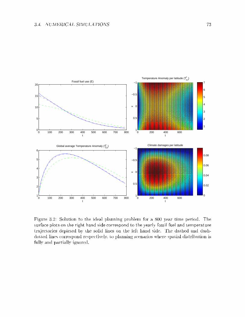
3.4. NUMERICAL SIMULATIONS 73
0 100 200 300 400 500 600 700 8000
5
10
15
20Fossil fuel use (E)
t
−1
−0.5
0
0.5
10 200 400 600
Temperature Anomaly per latitude (Tx,t+ )
t
x
1
2
3
4
5
6
7
0 100 200 300 400 500 600 700 8001
2
3
4
5
6
Global average Temperature Anomaly (T0,t+ )
t
−1
−0.5
0
0.5
10 200 400 600
Climate damages per latitude
t
x
0
0.02
0.04
0.06
0.08
Figure 3.2: Solution to the ideal planning problem for a 800 year time period. Thesurface plots on the right hand side correspond to the yearly fossil fuel and temperaturetrajectories depicted by the solid lines on the left hand side. The dashed and dash-dotted lines correspond respectively, to planning scenarios where spatial distribution isfully and partially ignored.

74 CHAPTER 3. EBCM'S AND THE CLIMATE-ECONOMY
We use this path to update the sum over k for and then keep repeating this procedureuntil convergence, which gives us the optimal paths for the planner.
Figure 3.2 shows the solution following the ideal planning problem over a 800 yeartime horizon. The left hand graphs depicts yearly fossil fuel use and the correspond-ing global temperature anomalies for three dierent modeling scenarios.47 The rstscenario, given by the solid blue lines of the upper and lower left hand graphs to-gether with the surface plots on the right, are based completely on the assumptionsdescribed in section 3.4.1. Here, the spatial distribution of temperatures, populationand damages are fully accounted for in the planners spatial and inter-temporal deci-sions on fossil fuel use . This implies that the planner weighs the social costs of agiven temperature increase at a particular location x according to the severity of dam-ages implied by our spatial damage function and the population size inhabiting thatspecic location. As can be seen optimal fossil fuel use falls over time. Compared tothe market outcome without taxes optimal fossil fuel use in the initial time period issubstantially lower than the global market outcome without taxes which would haveimplied a E0 = β0(1 − β)R0 ≈ 70GtC per year. The lower left hand graph describesthe corresponding temperature anomaly which peaks at ≈ 5.5C above year 1900 lev-els after about 240 years. The right hand side surface plots show the implications ofthese decisions for local temperature anomalies and climate damages for this scenario.The upper graph shows the temperature anomalies and as can be seen the temperatureanomaly grows larger at the poles as global average temperatures start to rise which isa consequence of diering temperature distributions for the base period compared tothe present as depicted in gure 3.1. As can be seen from inspection of the color chart,local temperatures have increased around one degree more at the poles compared to theglobal average and about one degree less than the global average at the equator after240 years. Turn now to climate damages in the graph below. Climate damages arecalculated as percent of GDP and the color chart displays damages varying from 0 to 9percent of local GDP. As can be seen, the gure displays a deep red spot in the middleshowing that damages in terms of GDP are substantially higher around the equatorthan at the poles. This is a consequence of the damage parameter θ(x) giving higherweights to tropical regions but also a consequence of population distribution. Carefulinspection of the surface plot shows that damages are actually slightly higher above theequator were the mean of the population distribution lies i.e. in the region below x = 0in the plot. Shifting the population distribution northward will thus increase damagesin northern regions.
46The solution to the fossil fuel use in decentralized equilibrium without taxes is entirely determinedby the discount rate and follows from Et+1 = βEt or alternatively Et = βt(1− β)R0.
47It should be noted that the results depicted here rely on several stylized assumptions regardingmodel specications and parameter choices and the results should thus not be interpreted as sayinganything in relation to whether current fossil fuel use is above or below optimal levels. In particular theassumption of freely available international transfers implicit in the ideal planning problem is indeedan extreme assumption. Further, the way fossil fuel is modeled is also very stylized and would alsoneed to be further rened.

3.5. CONCLUDING REMARKS 75
Next, concerning the other two scenarios. The left hand graphs also display adashed and a dash-dotted line. The dash-dotted line concerns the second scenario. Thisscenario could be seen as our equivalence of what Nordhaus does in his RICE model.Here, we consider an unequal distribution of damages and population across latitudes.However, compared to the rst scenario we have set the heat diusion coecient Dlarge enough so that temperature distribution across latitudes is essentially at as wasshown in proposition 3.1. Hence, in this scenario we are thus taking space into accountfrom a social perspective while ignoring temperature diusion implying that we are nowin the zero dimensional case which gives us a global average temperature as is also thecase in for example the RICE model. As can be seen this gives us a slightly lower initialvalue of fossil fuel use which also implies that the corresponding temperature trajectoryis slightly smoothed compared to the rst scenario. Finally, the third scenario, depictedby the dashed line, builds on the case where all latitude specic distributions have beenignored. In terms of Nordhaus models this case corresponds to his DICE model whereall global distribution issues are essentially ignored. This gives us an even lower pathof initial fossil fuel use and thus smooths out the temperature increase over time evenmore.
3.5 Concluding Remarks
In this paper we develop a model of climate change consisting of a one- dimensionalenergy balance climate model which is coupled with a model of economic growth. Webelieve that modeling heat transport in the coupled model is the main contribution ofour paper since it allows, for rst time as far as we know, the derivation of latitudedependent temperature and dam- age functions, as well as optimal mitigation policies,in the form of optimal carbon taxes, which are all determined endogenously throughthe interac- tion of climate spatiotemporal dynamics with optimizing forward lookingeconomic agents.
We derive Pareto optimal solutions for a social planner who seeks to implementoptimal allocations with taxes on fossil fuels and we show the links between welfareweights and international transfers across locations and the spatial structure of optimaltaxes. Our results suggest when per capita consumption across latitudes can be adjustedthrough costless transfers for any set of non negative welfare weights, so that marginalvaluations across latitudes are equated, or alternatively that transfers are zero due toNegishi weighting, then optimal carbon taxes will be spatially homogeneous. On theother hand when marginal valuations across latitudes are not equated, due to institu-tional/political constraints or the cost of transfers, optimal carbon taxes will instead bespatially dierentiated. We show that if international transfers are costly and the plan-ner is not constrained to by Negishi weighting, then taxes on fossil fuels could be lowerin relatively poor geographical areas. The degree of geographical tax dierentiation willdepend on the heat transport across latitudes. Without appropriate implementationof international transfers, and without Negishi weights that keep the existing interna-tional distribution invariant, carbon taxes will be latitude specic and their sizes will

76 CHAPTER 3. EBCM'S AND THE CLIMATE-ECONOMY
depend on the heat transfer across locations. We also show how to derive numericalresults for the optimization problem of the unconstrained planning problem with openmarkets. These results show how the optimization model can generate surface plots oftemperature and damages across latitudes and over time.
The climate module of our model is sometimes referred to as a surface EBCMwhere the impact of oceans is reected in the carbon decay parameter m, with nofurther modeling of the deep ocean component is undertaken. Further extensions of oursimple one-dimensional model to richer climate models (e.g. Kim and North (1992), Wuand North (2007)) with a ocean and with simple atmospheric layers added and wheretipping phenomena are possible may help understand results like those of Challenoret al. (2006), which found higher probabilities of extreme climate change than expected.Challenor et al. (2006) suggest several reasons for their ndings including "The mostprobable reason for this is the simplicity of the climate model, but the possibility existsthat we might be at greater risk than we believed". We emphasize that we are stilldoing what economists call a "nger exercise" in this paper where one deliberatelyposits an over simplied "cartoon" model in order to illustrate forces that shape, forexample, an object of interest like, a socially optimal fossil fuel tax structure overtime and space that might be somewhat robust to introduction of more realism intothe toy model. For example, we believe that the interaction of spatial heat transportphenomena and diculties in implementing income transfers (or their equivalent, e.g.allocations of tradeable carbon permits) will play an important role in determining theshape of the socially optimal tax schedule over dierent parts of space in more complexand more realistic models. Our simple model is useful in making this type of pointunder institutions where income transfers are possible and where they are politicallyinfeasible, i.e. essentially impossible.
The one-dimensional model allows the exploration of issues which cannot be fullyanalyzed in conventional zero-dimensional models. In particular one-dimensional mod-els with spatially dependent co-albedo allow the introduction of latitude dependeddamage reservoirs like endogenous ice-lines and permafrost. Since reservoir damagesare expected to arrive relatively early and diminish in the distant future, because thereservoir will be exhausted and sucient adaptation would have taken place, the tem-poral prole of the policy ramp could be declining, enforcing the result obtained forprot taxes, or even U-shaped.48 A U-shaped policy ramp could explained by the factthat as high initial damages due to the reservoir will start declining as the reservoiris exhausted, giving rice to a declining policy ramp, damages from the increase of theoverall temperature will dominate causing the policy ramp to become increasing. Thisis another potentially interesting and important area of further research.
48Judd and Lontzek (2011) have formulated a dynamic stochastic version of DICE, the SDICE - whichincludes stochastic tipping points possibilities. They show that this complexity aects the optimalpolicy results in comparison to RICE. Some of these issues are also explored in an accompanyingpaper of ours Brock et al. (2012a).

References
Anthoff D., 2011, Optimal Global Dynamic Carbon Abatement, http://www.
david-anthoff.de/Documents/AnthoffJobmarketPaper.pdf.
Archer D., 2005, Fate of fossil fuel CO2 in geologic time, Journal of GeophysicalResearch, vol. 110(C9), pp. 16.
Brock W., Engström G. and Xepapadeas A., 2012a, Energy Balance ClimateModels and the Spatial Structure of Optimal Mitigation Policies, beijer discussionpaper.
Brock W., Engström G. and Xepapadeas A., 2012b, One-Dimensional ClimateModels and Optimal Climate Policies across Locations, beijer discussion paper.
Budyko M.I., 1969, The eect of solar radiation variations on the climate of the earth,Tellus, vol. 21, pp. 61119.
Cai Y., Judd K.L. and Lontzek T.S., 2012, DSICE: A Dynamic Stochastic Inte-grated Model of Climate and Economy, rDCEP Working Paper No. 12-02.
Challenor P.G., Hankin R.K. and Marsh R., 2006, Towards the probability ofrapid climate change, pp. 5563, Cambridge University Press, Cambridge, UK., ch.7.
Chichilnisky G. and Heal G., 1994, Who should abate carbon emissions?: Aninternational viewpoint, Economics Letters, vol. 44, pp. 443449.
Chichilnisky G., Heal G. and Starrett D., 2000, Equity and Eciency in Envi-ronmental Markets: Global Trade in Carbon Dioxide Emissions, in G. Chichilniskyand G. Heal, eds., Environmental Markets: Equity and Eciency, New York:Columbia University Press.
Etheridge D., Steele L., Langenfelds R., Francey R., Barnola J.M. andMorgan V., 1998, Historical CO2 records from the Law Dome DE08, DE08-2, andDSS ice cores. In Trends: A Compendium of Data on Global Change., carbon DioxideInformation Analysis Center, Oak Ridge National Laboratory, U.S. Department ofEnergy, OakRidge, Tenn., U.S.A.
Golosov M., Hassler J., Krusell P. and Aleh T., 2011, Optimal taxes on fossilfuel in general equilibrium, Working Paper 17348, National Bureau of EconomicResearch.
Hansen J., Ruedy R., Sato M. and Lo K., 2010, Global surface temperature change,Review of Geophysics, vol. 48(RG4004), pp. 26979.
77

78 CHAPTER 3. EBCM'S AND THE CLIMATE-ECONOMY
Hansen J., Sato M., Kharecha P. and von Schuckmann K., 2011, Earth'senergy imbalance and implications, Atmospheric Chemistry and Physics, vol. 11, pp.1342113449.
Hassler J., Krusell P. and Olovsson C., 2011, Energy Saving Technical Change,mimeo, Institute of International Economic Studies, Stockholm University.
Held I.M.,Winton M., Takahashi K., Delworth T., Zeng F. and Vallis G.K.,2010, Probing the Fast and Slow Components of Global Warming by ReturningAbruptly to Preindustrial Forcing, Journal of Climate, vol. 23, pp. 2418242.
IPCC, 2001, Climate Change 2001: The Third Assessment Report of the Intergovern-mental Panel on Climate Change, Cambridge University Press, Cambridge.
IPCC, 2007, Climate Change 2007: The Fourth Assessment Report of the Intergovern-mental Panel on Climate Change, Cambridge University Press, Cambridge.
Judd K.L., 1998, Numerical Methods in Economics, vol. 2, MIT Press Books, TheMIT Press, 1 ed.
Judd K.L. and Lontzek T.S., 2011, Dynamic Stochastic General Equilibrium Analy-sis of Climate Change Policies, Conference presentation at INFORMS Annual Meet-ing - Austin, Texas.
Keen M. and Kotsogiannis C., 2011, Coordinating Climate and Trade Policies:Pareto Eciency and the Role of Border Tax Adjustments, CESIFO WORKINGPAPER NO. 3494, CATEGORY 1: PUBLIC FINANCE.
Kehoe T.J., Levine D.K. and Romer P.M., 1990, Determinacy of Equilibria in Dy-namic Models with Finitely Many Consumers, Journal of Economic Theory, vol. 50,pp. 121.
Kim K.Y. and North G., 1992, Seasonal cycle and second-moment statistics of asimple coupled climate system, Journal of Geophysical Research, vol. 97(20), pp.437448.
Knorr W., 2009, Is the airborne fraction of anthropogenic CO2 emissions increasing?,Geophysical Research Letters, vol. 36(L21710), pp. 15.
Knutti R., Krahenmann S., Frame D.J. and Allen M.R., 2008, Comment on'heat capacity, time constant, and sensitivity of earths climate system' by S. E.Schwartz, Journal of Geophysical Research, vol. 113(D15103).
Kummu M. and Varis O., 2011, The world by latitudes: A global analysis of humanpopulation, development level and environment across the north-south axis over thepast half century, Applied Geography, vol. 31(2), pp. 495507.

3.5. REFERENCES 79
Lindzen R.S. and Choi Y.S., 2009, On the determination of climate feedbacks fromERBE data, Geophysical Research Letters, vol. 36(16), pp. 16.
Lopez A., Smith L.A. and Suckling E., 2012, Pattern scaled climate scenarios:Are these useful for adaptation?, Centre for Climate Change Economics and Policy,Working Paper No. 80, Munich Re Technical Paper Number 13, Grantham ResearchInstitute on Climate Change and the Environment, Working Paper Number 71.
Nordhaus W.D., 2007, A Question of Balance, Yale University Press, New Haven &London.
Nordhaus W.D., 2010, Economic aspects of global warming in a post-Copenhagenenvironment., Proceedings of the National Academy of Sciences of the United Statesof America, vol. 107(26), pp. 1172126.
Nordhaus W.D., 2011, The architecture of climate economics: Designing a globalagreement on global warming, Bulletin of the Atomic Scientists, vol. 67(1), pp. 918.
Nordhaus W.D. and Boyer J., 2000, Warming the World: Economic Models ofGlobal Warming, MIT Press.
North G.R., 1975a, Analytical Solution to a Simple Climate Model with DiusiveHeat, Journal of Atmospheric Sciences, vol. 32, pp. 130107.
North G.R., 1975b, Theory of energy-balance climate models, Journal of AtmosphericSciences, vol. 32(11), pp. 203343.
North G.R., Cahalan R.F. and Coakley J.A., 1981, Energy Balance ClimateModels, Reviews of Geophysics and Space Physics, vol. 19(1), pp. 91121.
North G.R., Mengel J.G. and Short D.A., 1983, A Simple Energy Balance ModelResolving the Seasons and the Continents: Application to the Astronomical Theoryof the Ice Ages, Journal of Geophysical Research, vol. 88(6), pp. 5766.
Pierrehumbert R.T., 2008, Principles of Planetary Climate, Cambridge UniversityPress, UK.
Rogner H.H., 1997, An Assessment of World Hydrocarbon Resources, Annual Reviewof Energy and the Environment, vol. 22, pp. 217262.
Sandmo A., 2006, Global Public Economics: Public Goods and Externalities, Tech.Rep. 18-19, Revues.org.
Schneider T., von Deimling M., Meinshausen A., Levermann V., Huber K.,Frieler D., Lawrence M. and Brovkin V., 2011, Estimating the permafrost-carbon feedback on global warming, biogeosciences Discuss., 8, 47274761.

80 CHAPTER 3. EBCM'S AND THE CLIMATE-ECONOMY
Sellers W.D., 1969, A global climatic model based on the energy balance of theearth-atmosphere system, Journal of Applied Meteorology, vol. 8, pp. 392400.
Sellers W.D., 1976, A two-dimensional global climatic model, Monthly Weather Re-view, vol. 104, pp. 233248.
Shell K.M. and Somerville R.C.J., 2004, A generalized energy balance climatemodel with parameterized dynamics and diabatic heating, Journal of Climate, vol. 18,pp. 17531772.
Shiell L., 2003a, Descriptive, prescriptive and second-best approaches to the controlof global greenhouse gas emissions, Journal of Public Economics, vol. 87(7-8), pp.14311452.
Shiell L., 2003b, Equity and eciency in international markets for pollution permits,Journal of Environmental Economics and Management, vol. 46(1), pp. 3851.
Stanton E.A., 2010, Negishi welfare weights in integrated assessment models: themathematics of global inequality, Climatic Change, pp. 116.
Sterner T. and Persson U.M., 2008, An Even Sterner Review: Introducing RelativePrices into the Discounting Debate, Review of Environmental Economics and Policy,vol. 2(1), pp. 6176.
Tans P., 2011, Trends in Carbon Dioxide, nOAA/ESRL http://www.esrl.noaa.gov/
gmd/ccgg/trends/index.html.
Trenberth K.E., Fasullo J.T., O'Dell C. andWong T., 2010, Relationships be-tween tropical sea surface temperature and top-of-atmosphere radiation, GeophysicalResearch Letters, vol. 37(3), pp. 15.
Wu W. and North G.R., 2007, Thermal decay modes of a 2-D energy balance climatemodel, Tellus A, vol. 59(5), pp. 61826.
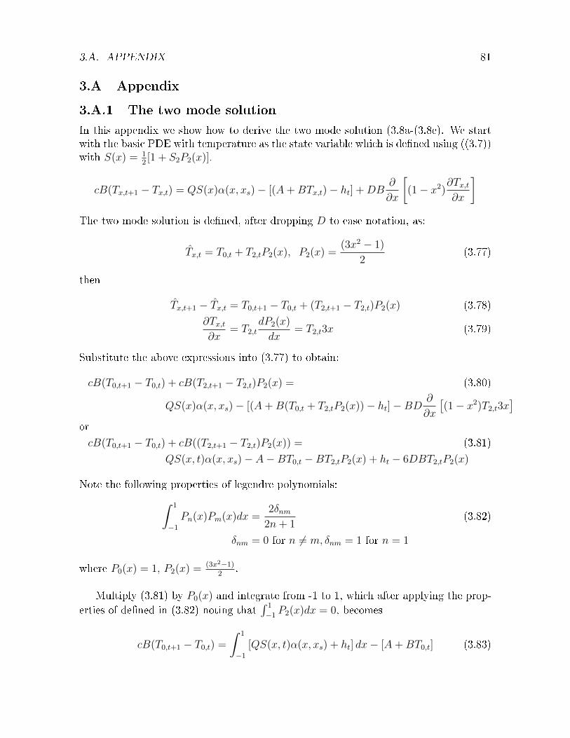
3.A. APPENDIX 81
3.A Appendix
3.A.1 The two mode solution
In this appendix we show how to derive the two mode solution (3.8a-(3.8e). We startwith the basic PDE with temperature as the state variable which is dened using ((3.7))with S(x) = 1
2[1 + S2P2(x)].
cB(Tx,t+1 − Tx,t) = QS(x)α(x, xs)− [(A+BTx,t)− ht] +DB∂
∂x
[(1− x2)
∂Tx,t∂x
]The two mode solution is dened, after dropping D to ease notation, as:
Tx,t = T0,t + T2,tP2(x), P2(x) =(3x2 − 1)
2(3.77)
then
Tx,t+1 − Tx,t = T0,t+1 − T0,t + (T2,t+1 − T2,t)P2(x) (3.78)∂Tx,t∂x
= T2,tdP2(x)
dx= T2,t3x (3.79)
Substitute the above expressions into (3.77) to obtain:
cB(T0,t+1 − T0,t) + cB(T2,t+1 − T2,t)P2(x) = (3.80)
QS(x)α(x, xs)− [(A+B(T0,t + T2,tP2(x))− ht]−BD∂
∂x
[(1− x2)T2,t3x
]orcB(T0,t+1 − T0,t) + cB((T2,t+1 − T2,t)P2(x)) = (3.81)
QS(x, t)α(x, xs)− A−BT0,t −BT2,tP2(x) + ht − 6DBT2,tP2(x)
Note the following properties of legendre polynomials:∫ 1
−1
Pn(x)Pm(x)dx =2δnm
2n+ 1(3.82)
δnm = 0 for n 6= m, δnm = 1 for n = 1
where P0(x) = 1, P2(x) = (3x2−1)2
.
Multiply (3.81) by P0(x) and integrate from -1 to 1, which after applying the prop-erties of dened in (3.82) noting that
∫ 1
−1P2(x)dx = 0, becomes
cB(T0,t+1 − T0,t) =
∫ 1
−1
[QS(x, t)α(x, xs) + ht] dx− [A+BT0,t] (3.83)

82 CHAPTER 3. EBCM'S AND THE CLIMATE-ECONOMY
Next, multiply (3.81) by P2(x) and integrate from -1 to 1, which after applying theproperties of dened in (3.82) noting that 〈P2(x), P2(x)〉 = 1
5we obtain
cB(T2,t+1 − T2,t) = −B(1 + 6D)T2,t(t) + 5
∫ 1
−1
QS(x, t)α(x, xs)P2(x)dx (3.84)
The ODEs (3.83) and (3.84) are the ODEs of the two mode solution which togetherwith (3.77) determine the two-mode solution. Substituting ht = ξ
2ln(1 + Mt
M
)into the
above gives us (3.8).
3.A.2 Static equilibrium
Start by dening Ψx(Tx,t) ≡ Ax,0LαLx,0Ω(Tx,t) so that
Yx,t = (anαL)t−1Ax,0LαLx,0Ω(Tx,t)K
αKx,t q
αqx,t = (anαL)t−1Ψx(Tx,t)K
αKx,t q
αqx,t
The lagrangian
L =
∫x
(anαL)t−1Ψx(Tx,t)(SKx,t)
αK (Sqx,t)αqdx
+ λK(1−∫x
SKx,tdx) + λq(1−∫x
Sqx,tdx)
The rst order conditions are
αK(anαL)t−1Ψx(Tx,t)(SKx,t)
αK−1(Sqx,t)αq = λK (3.85)
αq(anαL)t−1Ψx(Tx,t)(S
Kx,t)
αK (Sqx,t)αq−1 = λq (3.86)
Combining the rst order conditions we can after some algebra solve for SKx,t and SKx,t
SKx,t =λK
αK(anαL)t−1Ψx(Tx,t)
αq−1
αL λqαq(anαL)t−1Ψx(Tx,t)
−αqαL
Sqx,t =λq
αq(anαL)t−1Ψx(Tx,t)
αK−1
αL λKαK(anαL)t−1Ψx(Tx,t)
−αKαL
Next, substitute these expressions into their respective constraints we can write
1 =
∫x
SKx,tdx =λK
αK(anαL)t−1
αq−1
αL λqαq(anαL)t−1
−αqαL
∫x
Ψx(Tx,t)1αL dx
1 =
∫x
Sqx,tdx =λq
αq(anαL)t−1
αK−1
αL λKαK(anαL)t−1
−αKαL
∫x
Ψx(Tx,t)1αL dx
after substituting back in the conditions (3.85) and (3.86) into these expressions wehave that
SKx,t = Sqx,t = Ψx(Tx,t)1αL /
∫x
Ψx(Tx,t)1αL dx

3.A. APPENDIX 83
Next, after substituting these optimality shares back into the objective function itfollows that
Ftotal(Kt, qt, Tx,tx=1x=−1 ; t) = (anαL)t−1KαK
t qαqt
∫x
Ψx(Tx,t)Ψx(Tx,t)
1αL∫
xΨx(Tx,t)
1αL dx
αK+αq
dx
= (anαL)t−1KαKt q
αqt
(∫x
Ψx(Tx,t)1αL dx
)αL3.A.3 Proof that the planning problem with costly transfers can
be represented by a competitive equilibrium.
For the case of costly transfers we for simplicity ignore bonds and modify the consumersproblem as follows
max∞∑t=0
βtLx,tU(Cx,t/Lx,t) (3.87)
subject to∞∑t=0
pkt (Cx,t +Kx,t+1) =∞∑t=0
pkt (Rx,tKx,t + Ix,t −Θx,t) (3.88)
Θx,t ≡C0
2(Rx,tKx,t + Ix,t −Kx,t+1 − Cx,t)2 (3.89)
Ix,t ≡ wx,tLx,t + ptqx,t + τx,tqx,t (3.90)
From the rst order necessary condition for consumption and capital we have
U ′(Cx,t/Lx,t) = Λkxp
kt [1−Θ′x,t] (3.91)
Rx,t+1 =pkt [1−Θ′x,t]
βpkt+1[1−Θ′x,t+1](3.92)
The assumptions regarding the consumption goods producing rms stay the same as insection 3.3.4 with the exception that fossil fuel prices are now due to the adjustmentcosts, latitude dependent, and given by px,t so that the rst order condition w.r.t qx,tinstead is given by Ax,tΩ(Tx,t)F
′q(Kx,t, Lx,t, qx,t) = px,t + τx,t. The fossil rms also face
latitude specic prices px,t and interest rates Rx,t which implies that their rst orderconditions now satisfy px,t+1 = Rx,t+1px,t. Based on these revised assumptions of thecompetitive equilibrium it is clear that both the Euler equation and the externalityadjusted Hotelling rule of the planning problem can be produced by the rst orderconditions of the competitive equilibrium given that taxes are set to
τx,t =σλmt
λkt [1−Θ′x,t](3.93)
Next, we note that by inserting the rst order conditions of the consumption goodproducers into the adjustment cost function and budget constraint of the representative
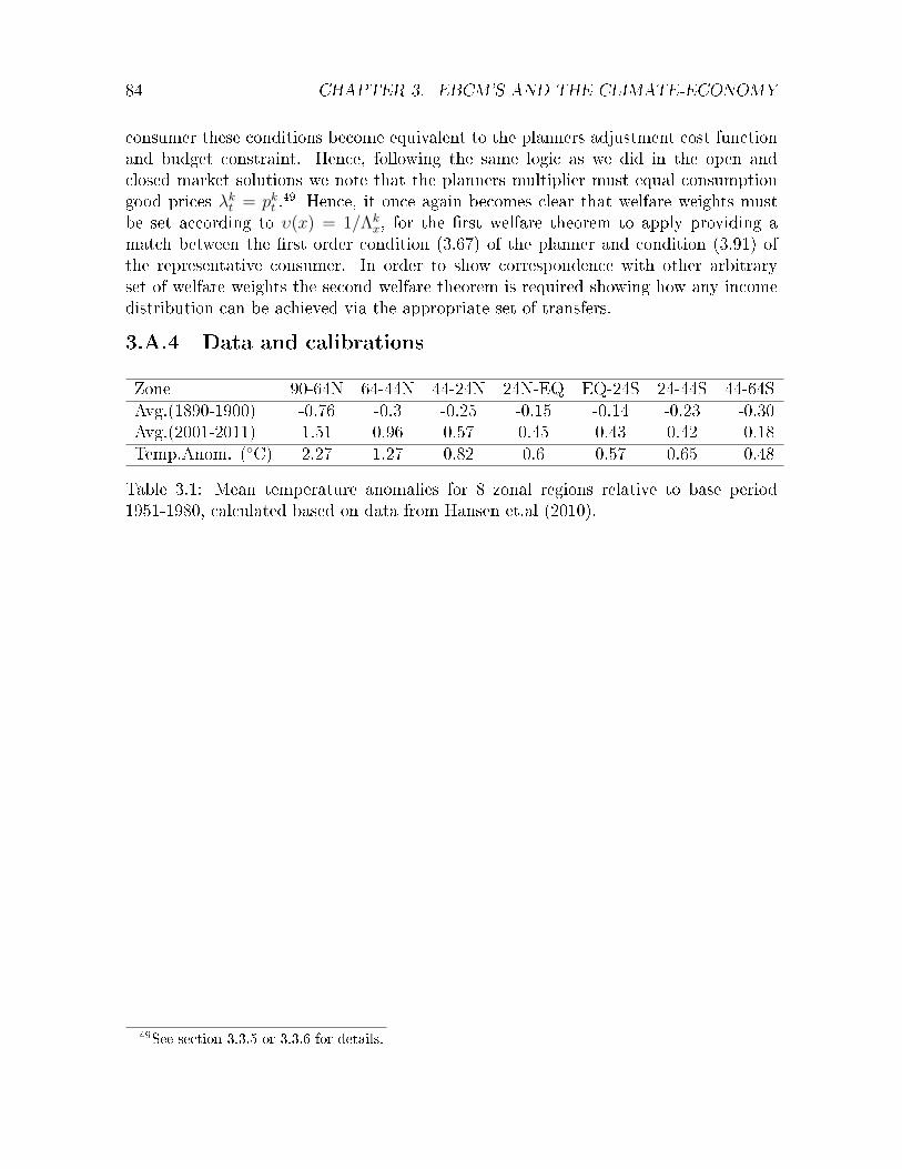
84 CHAPTER 3. EBCM'S AND THE CLIMATE-ECONOMY
consumer these conditions become equivalent to the planners adjustment cost functionand budget constraint. Hence, following the same logic as we did in the open andclosed market solutions we note that the planners multiplier must equal consumptiongood prices λkt = pkt .
49 Hence, it once again becomes clear that welfare weights mustbe set according to υ(x) = 1/Λk
x, for the rst welfare theorem to apply providing amatch between the rst order condition (3.67) of the planner and condition (3.91) ofthe representative consumer. In order to show correspondence with other arbitraryset of welfare weights the second welfare theorem is required showing how any incomedistribution can be achieved via the appropriate set of transfers.
3.A.4 Data and calibrations
Zone 90-64N 64-44N 44-24N 24N-EQ EQ-24S 24-44S 44-64SAvg.(1890-1900) -0.76 -0.3 -0.25 -0.15 -0.14 -0.23 -0.30Avg.(2001-2011) 1.51 0.96 0.57 0.45 0.43 0.42 0.18Temp.Anom. (C) 2.27 1.27 0.82 0.6 0.57 0.65 0.48
Table 3.1: Mean temperature anomalies for 8 zonal regions relative to base period1951-1980, calculated based on data from Hansen et.al (2010).
49See section 3.3.5 or 3.3.6 for details.

Chapter 4
Energy Balance Climate Models,
Damage Reservoirs and the Time
Prole of Climate Change Policy∗
4.1 Introduction
Energy balance climate models (EBCMs) have been extensively used to study Earth'sclimate (e.g. Budyko (1969), Sellers (1969), North (1975a), North (1975b) , Northet al. (1981)), and Wu and North (2007)). The basic components of these models areincoming solar radiation, outgoing infrared radiation, transportation of heat across theglobe and the presence of an endogenous ice line where latitudes north (south) of theice line are solid ice and latitudes south (north) of the ice line are ice free. The iceline has the important property of regulating the planets energy heat budget where thelocation of the ice line determines how much of the incoming solar radiation is reectedback out to space. Ice covered areas have a higher albedo implying that they absorbless of the incoming solar radiation thus contributing less to planetary warming.
In the economics literature, climate change is often studied in the framework of in-tegrated assessment models (IAMs) featuring carbon cycles and temperature dynamics(e.g. Nordhaus (1994), Tol (1997) Nordhaus and Boyer (2000), Hope (2006), Nordhaus(2007)). These models typically feature empirically calibrated, to the most part linear,climate modules capturing global average estimates of for example atmospheric tem-perature levels. This approach tends to ignore the complexities associated with heattransportation across latitudes and ice-albedo feedback eects which lie at the heart ofthe EBCM literature.1 The importance of ice-albedo feedback eects and latitudinalheat transportation in regulating the climate was recognized early in eorts to repre-sent the earths climate with EBCM's which uncovered the disconcerting possibilitythat a relatively small decrease in the solar input could lead to catastrophic global
∗This paper has been co-authored with William A. Brock and Anastasios Xepapadeas1In this context, the ice-albedo feedback refers to a process allowing the surface albedo to vary with
the climate state.
85
86 CHAPTER 4. ECONOMIC-EBCM'S AND DAMAGE RESERVOIRS
glaciation, the result of a runaway ice albedo feedback (North, 1984). Similarly it wasalso shown that the ice-albedo feedback eect could have an equally strong amplifyingeect on the climate when driven by increasing concentrations of atmospheric carbondioxide (Wang and Stone, 1980). This showed how something happening at one par-ticular latitude, the albedo changing due to ice line movements, could act to aect theglobal mean climate. Such feedback eects have also been associated with the notionof climate "tipping points" dened as points where a small forcing is enough to set of achain of interactions causing a major change in behavior of the system (Roe and Baker,2010). The potential threats associated with such tipping points has raised much con-cern within the climate science community in recent years (see e.g. Kerr (2008); Lentonet al. (2008); Smith et al. (2009)).
In the present paper we couple a latitude dependent EBCM with an endogenous iceline based on the model by North (1975a,b), with a simplied economic growth model.This allows us to investigate what new insights might be gained regarding the timeprole of mitigation policy and distribution of damages when accounting for increasedcomplexitity in terms of the ice-albedo feedback and latitudinal heat transport. Theexplicit presence of a spatial dimension and an ice line, whose latitude is determinedendogenously, also suggests a dierent damage prole for sources of damages connectedto the movement of the ice line. This does not appear in traditional IAMs. In partic-ular, we dierentiate between two types of damages from climate change, traditionalgradually increasing damages, and a damage reservoir type, where the later represents anite source of economic damage associated with the movement of the ice line. Damagereservoirs in the context of climate change can be regarded as sources of damage whicheventually will cease to exist when the source of the damage has been depleted. Weidentify, ice caps and permafrost as typical damage reservoirs, where the state of thereservoir is connected to the latitudinal position of the ice line.
Concerning the ice caps, the movement of the ice line closer to the poles is clearlyconnected to shrinking ice caps. We consider the implied damages caused by sea levelrise due to the release of water from melting glacial ice sheets. We might expectthat marginal damages from melting ice caps will increase slowly at rst, acceleratingto a peak but then eventually diminish as the ice line approaches the Poles. Whenthere is no ice left on the Poles this damage reservoir will have been exhausted. Theexact shape of an ice cap specic damage function is of course unknown, it might aswell be that damages are proportional to the size of the ice caps so that marginaldamages are initially high but diminish as more ice is melted.2 However, regardless
2Damages due to sea level rise also depend on the shape of the shoreline which will determine theamount of land to be covered by water due to melting ice caps (see e.g. the study by Li et al. (2009)).Further sea level rise can also be caused by thermal expansion of warming oceans, as a direct result ofa rising global temperature. Which of these eects dominate depends upon the time scale studied. Forexample, the Intergovernmental Panel on Climate Change's Fourth Assessment Report (IPCC (2007))concluded that thermal expansion can explain about 25 percent of observed sea-level rise for 1961-2003and 50 percent for 1993-2003, but with considerable uncertainty. There may of course also be otherdamages caused by the increasing loss of the ice caps and their role in regulating the climate.

4.1. INTRODUCTION 87
of the intermediate behavior, claiming that marginal damages due to ice melting musteventually be zero when all ice has melted is hardly controversial. Thus as humanactivities move the ice line towards the North Pole the ice area lost diminishes andmarginal damages diminish also. The presence of an endogenous ice line in the EBCMallows us to model this type of damages explicitly given the relevant information.3
Permafrost is also related to damage reservoirs. Permafrost or permafrost soil is soilat or below the freezing point of water ( 0 C or 32 F) for two or more years. Permafrostregions occupy approximately 22.79 million square kilometers (about 24 percent of theexposed land surface) of the Northern Hemisphere (Zhang et al. (2003)). Permafrostoccurs as far north as 84 N in northern Greenland, and as far south as 26 N in the Hi-malayas, but most permafrost in the Northern Hemisphere occurs between latitudes of60 N and 68 N. (North of 67 N, permafrost declines sharply, as the exposed land sur-face gives way to the Arctic Ocean.) Recent work investigating the permafrost carbonpool size estimates that 1400-1700 Gt of carbon is stored in permafrost soils worldwide.This large carbon pool represents more carbon than currently exists in all living thingsand twice as much carbon as exists in the atmosphere (Tarnocai et al. (2009)). Thethawing of permafrost as high latitudes become warmer can also be modeled in thiscontext. Thawing of permafrost is expected to bring widespread changes in ecosystems,increase erosion, harm subsistence livelihoods, and damage buildings, roads, and otherinfrastructure. Loss of permafrost will also cause release of greenhouse gases, methanein wetter areas and CO2 in dryer areas. Furthermore, permafrost damages are related todamage reservoirs since when permafrost is gone they will vanish provided appropriateadaptation has been implemented.4 Once again the exact shape of the damage functionin the intermediate is unknown, but it is clear that damages must eventually diminishonce all greenhouse gases trapped in the soil has been released. The permafrost feed-back also suggests that permafrost carbon emissions could aect long-term projectionsof future temperature change. An increase in Arctic temperatures could release a largefraction of the carbon stored in permafrost soils. Studies indicate that up to 22% ofpermafrost could be thawed already by 2100. Once unlocked under strong warming,thawing and decomposition of permafrost can release amounts of carbon until 2300
3Scientic evidence seems to support the argument that ice sheets might be seriously aected byrelatively low increases in temperature. Oppenheimer (2005) reports a number of results suggestingthat both the Greenland Ice Sheet (GIS) and the West Antarctic Ice Sheet (WAIS) could be highlyvulnerable to temperature rise within the range studied by the current IAMs. Oppenheimer and Alley(2004) report that a 2-4C global mean warming could be justied for WAIS. Carlson et al. (2008)conclude that geologic evidence for a rapid retreat of the Laurentide ice sheet, which is the mostrecent (early Holocene epoch) and best documented disappearance of a large ice sheet in the NorthernHemisphere, may describe a prehistoric precedent for mass balance changes of the Greenland Ice Sheetover the coming century. In a recent report from the European Energy Agency Agency (2010), itwas stated that one of the potential large-scale changes likely to aect Europe is the deglaciation ofthe WAIS and the GIS and that there is already evidence of accelerated melting of the GIS. Further,a sustained global warming in the range of 1-5C above 1990 temperatures, could generate tippingpoints leading to at least partial deglaciation of the GIS and WAIS, thus implying a signicant rise insea levels. See also Lindsay and Zhang (2005).
4For more details see for example Zhang et al. (2003), Zimov et al. (2006), Schaefer et al. (2011).

88 CHAPTER 4. ECONOMIC-EBCM'S AND DAMAGE RESERVOIRS
comparable to the historical anthropogenic emissions up to 2000 (approximately 440GtC) (von Deimling et al. (2011)).
To the best of our knowledge, we believe this to be the rst attempt at introducingan explicit spatial dimension to the climate module of a climate-economy model whichalso connects the spatial aspects to the temporal prole of climate damages. This helpsin understanding how latitude dependent damages might aect decision-making relatedto climate change. To be more precise, by allowing for damage reservoirs, as describedabove, we explicitly introduce two types of damage functions having dierent tempo-ral proles. These are the traditional damage function used in most IAMs, in whichdamages increase monotonically with temperature, and a damage function associatedwith damage reservoirs. The damage reservoir function is given a similar form as thetraditional damage function with the exception that there exist a point where marginaldamages will start to decline and eventually become zero implying that damages arebounded from above. This is related to the idea that once the ice caps are gone andthe thawed permafrost has released most of its carbon, then reservoir damages will beexhausted. Our results suggest that endogenous ice lines and damage reservoirs intro-duce non-convexities which induce multiple steady states and Skiba points. The policyimplication of these results is that when damage reservoirs are ignored we have a uniquesteady state and the policy ramp is monotonically increasing. That is, carbon taxesstart at low levels and increase with time, which is the `gradualist approach' to climatepolicy Nordhaus (2007), Nordhaus (2010), Nordhaus (2011). On the other hand theexistence of damage reservoirs and multiple steady states induced by endogenous icelines results in policy ramps which suggest increased mitigation now, the opposite ofwhat is advocated by the gradualist approach. Furthermore by incorporating damagereservoirs into a DICE type model, our simulations suggest a u-shaped policy rampwith high mitigation now.5
The rest of the paper is structured as follows. Since EBCMs are new in economicswe proceed in steps that we believe make this methodology accessible to economists.In section 4.2 we present a basic energy balance climate model6 which incorporateshuman impacts on climate which result from carbon dioxide emissions that eventuallyblock outgoing radiation. In developing the model we follow (North (1975a), North(1975b)) and use his notation. Section 4.3 couples the spatial EBCM with an economicgrowth model characterized by both traditional and reservoir damages. We show thatnonlinearities induced by endogenous ice lines and reservoir damages result in multiplesteady states and Skiba points. Section 4.4 derives similar results in a model moresimilar in structure to most IAM's. Finally, in section 4.5 we simulate the well known
5Multiple equilibria and high current mitigation are also suggested by models incorporating un-certain climate thresholds into DICE (Keller et al. (2004), Lempert et al. (2006)). See also Nævdal(2006) for an optimal control version featuring uncertain thresholds. More recently Judd and Lontzek(2011) have formulated a dynamic stochastic version of DICE which they call DSICE. They also extendtheir model to include stochastic tipping point possibilities. They show how this additional real worldcomplexity substantially aects the optimal policy results in comparison to DICE.
6For more on EBCMs, see for example Pierrehumbert (2011).

4.2. A SIMPLIFIED ONE-DIMENSIONAL EBCM 89
DICE model allowing for damage reservoirs and derive a u-shaped policy ramp. Thelast section concludes.
4.2 A Simplied One-dimensional Energy Balance Climate Model
In this section we present a simplied integrated model of economy and climate, withthe climate part motivated by the one-dimensional energy balance models described inthe introduction. The term one-dimensional means that there is an explicit spatialdimension in the model, measured in terms of latitudes. The important feature ofthese models is that they allow for heat diusion or transportation across latitudeswhich increases the relevance of the models in describing climate dynamics. Let T (x, t)denote the surface temperature at location (or latitude) x and time t measured in C.Climate dynamics in the context of the ECBM (e.g. North (1975a,b), North et al.(1981)) are dened as:
B∂T (x, t)
∂t= QS(x)α(x, xs)− [A+BT (x, t)− g(M(t))]
+D∂
∂x
[(1− x2)B
∂T (x, t)
∂x
](4.1)
Ts = T (xs(t), t) (4.2)
where x denotes the sine of the latitude x, where units of x are chosen so that x = 0denotes the Equator, x = 1 denotes the North Pole7 and to simplify we just refer tox as latitude. A and B are constants which are used to relate the outgoing longwave infrared radiation ux I(x, t) measured in W/m2 at latitude x at time t with thecorresponding surface temperature T (x, t) through the empirical formula,8
I(x, t) = A+BT (x, t) (4.3)
g(M(t) denotes forcing induced by the atmospheric CO2 concentration given by M(t).A common form for g(M(t) is a logarithmic form identifying the amount of globalwarming that can be induced from a doubling CO2 levels.9 For the qualitative exercisewe pursue in this paper we will however assume a simple linear form in order to keeptechnicalities to a minimum. More about this below. Q is the solar constant divided by4.10 As pointed out by North (1975b), in equilibrium at a given latitude the incoming
7Symmetry for the part x ∈ [−1, 0] is assumed. This assumption is common in EBCMs.8It is important to note that the original Budyko (1969) formulation cited by North parameterizes
A,B as functions of fraction cloud cover and other parameters of the climate system. North (1975b)points out that due to non-homogeneous cloudiness A and B should be functions of x. There isapparently a lot of uncertainty involving the impact of cloud dynamics (e.g. Trenberth et al. (2010)versus Lindzen and Choi (2009)). Hence robust control in which A,B are treated as uncertain maybe called for but this is left for further research. Example, of values used by North (1975a) areA = 201.4W/m2, B = 1.45W/m2.
9See for example table 6.2 of the IPCC (2001) report.10The solar constant includes all types of solar radiation, not just the visible light. It is measured
by satellite to be roughly 1.366 kilowatts per square meter (kW/m2).

90 CHAPTER 4. ECONOMIC-EBCM'S AND DAMAGE RESERVOIRS
absorbed radiant heat is not matched by the net outgoing radiation and the dierenceis made up by the meridional divergence of heat ux which is modeled by the termD ∂
∂x
[(1− x2)B ∂T (x,t)
∂x
]. Several forms are possible here, the seminal contributions by
Budyko (1969) and Sellers (1969) both dier in their parametrizations and structureof heat diusion. Our form follows that of North (1975a,b) featuring a single thermaldiusion coecient D which is a calibration parameter determining both heat diusionand temperature anomalies across latitudes.11 S(x, t) is the mean annual meridionaldistribution of solar radiation which is determined from astronomical calculations andban be uniformly approximated within 2% by
S(x) = 1 + S2P2(x) (4.4)
with S2 = −0.482 and where P2(x) = (3x2 − 1)/2 is the second Legendre polynomial(North, 1975a). Note that S(x) has been normalized so that its integral from 0 to 1 isunity which implies that the integral of incoming radiation reaching the earth is givenby Q. α(x, xs(t)) is the absorption coecient which equals one minus the albedo ofthe earth-atmosphere system, with xs(t) being the latitude of the ice line at time t. Inequation (4.5) below the ice line absorption drops discontinuously because the albedojumps discontinuously. North (1975b), page 2034, equation (3) species this co-albedofunction as:12
α(x, xs) =
b0 = 0.38 x > xs
α0 + α2P2(x)x < xs,
α0 = 0.697α2 = −0.0779.
(4.5)
where P2(x) = (3x2 − 1)/2 represents the second Legendre polynomial. In this set-upthe ice line is determined dynamically by the following condition from (Budyko (1969),North (1975a,b)):
T > −10oCno ice line presentT < −10oC ice present (4.6)
nally equation (4.2) determines the location of the ice line (xs(t)). Given the abovespecication the temperature (Ts) constitutes a break even temperature where tem-peratures below this level are assumed to be ice covered over the whole year and viceversa. Hence, by setting Ts = −10 as in Budyko and North we can solve the equationTs = T (xs(t), t) for xs(t) which is needed in order to determine the solution to (4.1)for given levels of atmospheric carbon dioxide M(t). Equation (4.1) thus states thatthe temperature at any given latitude is determined by the dierence in incoming so-lar radiation QS(x)α(x, xs) and outgoing radiation heat radiation I(x, t) adjusted forlatitudinal heat ux D ∂
∂x[. . .].
Although the introduction of heat diusion adds extra complexity, since it denedthrough the use of partial dierential equations, a more simplied approach is available
11As an example of the magnitude of D, North et al. (1981) pick a value of D = 0.649.12A smoothed version of a co-albedo function is equation (38) of North et al. (1981).

4.2. A ONE-DIMENSIONAL ECONOMIC-EBCM 91
through the use of Legendre approximation methods as introduced by (North (1975b)).The solution can then be approximated by
T (x, t) =∑nEven
Tn(t)Pn(x) (4.7)
where Tn(t) are solutions to appropriately dened ODEs and Pn(x) are even numberedLegendre polynomials. A satisfactory approximation of the solution for (4.1)-(4.2)within a few percent, can be obtained by the so called two mode solution where n =0, 2 (North, 1975b).13 The two-mode approximation is thus dened as T (x, t) =T0(t) + T2(t)P2(x) where T0(t), is the rst mode, and T2(t), the second mode. Hence,a two-mode approximation to the system (4.1)-(4.2) can be obtained from the solutionto the following system of dierential algebraic equations:
BdT0
dt= −(A+BT0(t)) +
∫ 1
0
QS(x)α(x, xs(t))dx+ g (M (t)) (4.8)
BdT2
dt= −(1 + 6D)BT2(t) + 5
∫ 1
0
QS(x)α(x, xs(t))P2(x)dx (4.9)
T (x, t) = T0(t) + T2(t)P2(x) (4.10)T (xs, t) = Ts (4.11)
where P2(x) = (3x2− 1)/2 is the second Legendre polynomial that provides the spatialdimension to the solution. Note, that the constant ice line temperature Ts = −10 isneeded in order to determine the position of the ice line xs and hence the co-albedoα(x, xs(t)) of (4.8) and (4.9).
From the two-mode approximation of the temperature, we obtain the global meantemperature T0(t), which is just the integral of T (x, t) over x from zero to one. Thevariance of the temperature can be dened as
VT =
∫ 1
0
[T (x, t)− T0(t)]2 dx =
∫ 1
0
(T2(t)P2(x))2dx =(T2(t))2
5(4.12)
Local temperature means at latitudes (x, x+ dx) and the mean temperature over aset of latitudes, Z = [a, b], are dened by
[T0(t) + T2(t)P2(x)] dx, m [a, b] =
∫ b
a
[T0(t) + T2(t)P2(x)] dx (4.13)
while the variance of temperature over the set of latitudes Z = [a, b] is
V [a, b] =
∫ b
a
[T0(t) + T2(t)P2(x)−m [a, b; t]]2 dx. (4.14)
13The complete derivation of the two-mode solution is provided in Appendix 4.A. For more detailsregarding the use of approximation methods see chapter 6 of Judd (1998).

92 CHAPTER 4. ECONOMIC-EBCM'S AND DAMAGE RESERVOIRS
When the area Z = [a, b] is introduced, it is plausible to assume that utility in eacharea [a, b] depends upon both the mean temperature and the variance of temperaturein that area. For example we may expect increases in mean temperature and varianceto have negative impacts on output in any area Z, if it is located in tropical latitudes.In contrast mean temperature increases in some areas Z (e.g. Siberia) may increaserather than decrease utility.14 Existing dynamic IAMs cannot deal with these kindsof spatial elements, such as impacts of changes in temperature variance, generated byclimate dynamics over an area Z.
In the climate modelM (t) is the stock of the atmospheric carbon dioxide. This stockaects the evolution of the temperature through the function g, and evolves throughtime under the forcing of human inputs in the form of emissions of green house gases(GHGs) h(x, t) emitted at latitude x and time t.
For the human input we assume that emissions h (x, t) relate to S (t) by the simpleequation
M (t) =
∫ 1
0
h(x, t)dx−mM (t) = h (t)−mM (t) (4.15)
where m is the carbon decay rate. To simplify the exposition we reduce the numberof state variables in the problem by assuming that M (t) has relaxed to a steady stateand it relates to h (t) through the simple linear relation M (t) = (1/m)h (t) . Thus weapproximate g (M (t)) by a simple linear relation γh (t).15In this model the latitudeof the ice line can move in time in response to changes in human input since the iceline solution depends on h(t). Moving of the ice line towards the poles generates thedamages related to damage reservoirs.
The climate model (4.8)-(4.11) that incorporates human input, which aects the evo-lution of temperature can be further simplied by following simplications proposed byWang and Stone (1980) which suggest that an approximation for the solution equa-tion T (x, t) = T0(t) + T2(t)P2(x) can be achieved by replacing T2(t) by an appropriateconstant. Then dT (x, t)/dt = dT0(t)/dt, where T0(t), is global mean surface (sea level)temperature. Writing T (t) = T0(t) the evolution of the global mean temperature canbe approximated by:
dT (t)
dt= −A
B− T (t) +
1
B
∫ 1
0
[QS(x)α(x, xs(t))] dx+ g (M(t)) . (4.16)
Thus the Wang and Stone (1980) approximation reduces the model to one whoseevolution is described by (4.16). Wang and Stone (1980) (equation 3) calibrate the
14Here, we are referring to variance across latitudes. In a stochastic generalization of our model, wecould introduce a stochastic process to represent weather, i.e. very high frequency uctuations relativeto the time scales we are modeling here. Here the local variance of high frequency phenomena likeweather may change with changes in lower frequency phenomena such as mean area Z temperatureand area Z temperature variance. See North et al. (1981) for an example of how stochastic forcing canbe modeled in an EBM framework. We leave this task to future research.
15More complicated and probably more realistic approximations will not aect our qualitative resultsregarding the multiplicity of steady states and the emergence of Skiba points.

4.3. DAMAGE RESERVOIRS AND MULTIPLE STEADY STATES 93
model to get a simple equation for the ice line
xs(t) = (aice + biceT (t))1/2, aice = 0.6035, bice = 0.02078. (4.17)
4.3 The Economic-Climate Model: Damage Reservoirs and Mul-
tiple Steady States
We introduce the two types of damages due to climate change mentioned earlier. Letus dene these damages by two functions D1(T (t)) and D2(xs(t)), where 1 denotes thetraditional damages due to temperature rise, and 2 denotes damages due to reservoirdamages from movement of the ice line towards the north and permafrost melting. Asimplied integrated EBCM can be developed along the following lines.
We consider a simplied economy with aggregate capital stock K. An amount K2
from this capital stock is diverted to alternative clean technologies. Output in theeconomy is produced by capital and emissions h according to a standard productionfunction F (K − K2, h + φK2), where φ is an eciency parameter for clean technolo-gies.16 The cost of using a unit of h is Ch(h),with Ch(0) = 0, C
′
h > 0, C′′
h > 0. Theuse of emissions can be reduced by employing clean technologies at an eective rateφK2. Denoting consumption by C, net capital formation in our simplied economy isdescribed by
dK
dt= F (K −K2, h+ φK2)− C − Ch(h)− δK (4.18)
where δ is the depreciation rate on the capital stock. Assuming a linear utility functionor U(C) = C, we consider the problem of a social planner that seeks to maximizediscounted life time consumption less damages from climate change subject to (4.16),(4.17), and (4.18).
In this set-up the problem of the social planner can be described, in terms of the
16See Xepapadeas (2005) for dierent ways in which emissions and environment can be modeled asproduction factors.
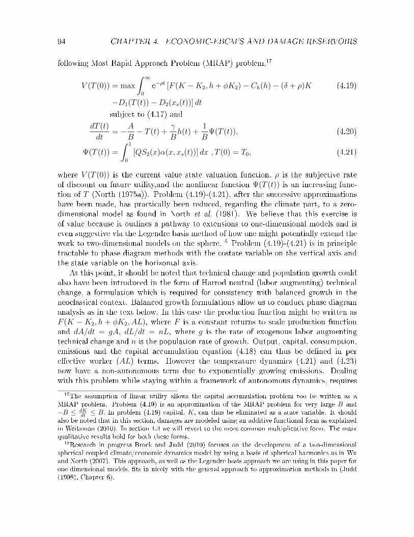
94 CHAPTER 4. ECONOMIC-EBCM'S AND DAMAGE RESERVOIRS
following Most Rapid Approach Problem (MRAP) problem,17
V (T (0)) = max
∫ ∞0
e−ρt [F (K −K2, h+ φK2)− Ch(h)− (δ + ρ)K (4.19)
−D1(T (t))−D2(xs(t))] dt
subject to (4.17) anddT (t)
dt= −A
B− T (t) +
γ
Bh(t) +
1
BΨ(T (t)), (4.20)
Ψ(T (t)) =
∫ 1
0
[QS2(x)α(x, xs(t))] dx , T (0) = T0, (4.21)
where V (T (0)) is the current value state valuation function, ρ is the subjective rateof discount on future utility,and the nonlinear function Ψ(T (t)) is an increasing func-tion of T (North (1975a)). Problem (4.19)-(4.21), after the successive approximationshave been made, has practically been reduced, regarding the climate part, to a zero-dimensional model as found in North et al. (1981). We believe that this exercise isof value because it outlines a pathway to extensions to one-dimensional models and iseven suggestive via the Legendre basis method of how one might potentially extend thework to two-dimensional models on the sphere.18 Problem (4.19)-(4.21) is in principletractable to phase diagram methods with the costate variable on the vertical axis andthe state variable on the horizontal axis.
At this point, it should be noted that technical change and population growth couldalso have been introduced in the form of Harrod neutral (labor augmenting) technicalchange, a formulation which is required for consistency with balanced growth in theneoclassical context. Balanced growth formulations allow us to conduct phase diagramanalysis as in the text below. In this case the production function might be written asF (K − K2, h + φK2, AL), where F is a constant returns to scale production functionand dA/dt = gA, dL/dt = nL, where g is the rate of exogenous labor augmentingtechnical change and n is the population rate of growth. Output, capital, consumption,emissions and the capital accumulation equation (4.18) can thus be dened in pereective worker (AL) terms. However the temperature dynamics (4.21) and (4.23)now have a non-autonomous term due to exponentially growing emissions. Dealingwith this problem while staying within a framework of autonomous dynamics, requires
17The assumption of linear utility allows the capital accumulation problem too be written as aMRAP problem. Problem (4.19) is an approximation of the MRAP problem for very large B and−B ≤ dK
dt ≤ B. In problem (4.19) capital, K, can thus be eliminated as a state variable. It shouldalso be noted that in this section, damages are modeled using an additive functional form as explainedin Weitzman (2010). In section 4.4 we will revert to the more common multiplicative form. The mainqualitative results hold for both these forms.
18Research in progress Brock and Judd (2010) focuses on the development of a two-dimensionalspherical coupled climate/economic dynamics model by using a basis of spherical harmonics as in Wuand North (2007). This approach, as well as the Legendre basis approach we are using in this paper forone-dimensional models, ts in nicely with the general approach to approximation methods in (Judd(1998), Chapter 6).

4.3. MULTIPLE STEADY STATES 95
introduction of emission reducing technological progress at an appropriate rate in orderto be able to transform the temperature dynamics into a stationary form so that phasediagram techniques of analysis of autonomous systems can still be applied. However,this is beyond the scope of the current paper. In the current paper we wish to show howspatial EBCMs can be integrated with capital accumulation models in economics whilepreserving analytical tractability. The time stationary analysis developed here indicatesthat a full analysis of more realistic non-stationary systems is potentially tractable nowthat we have pointed the way in this paper.
Returning to our time stationary framework, we feel that insights are gained morerapidly by analyzing the following qualitatively similar problem that is strongly moti-vated by the problem (4.19)-(4.21):
V (T (0)) = max
∫ ∞0
e−ρt [F (K −K2, h+ φK2)− Ch(h)− (δ + ρ)K (4.22)
−D1(T )−D2(T )] dt
s.t.dT
dt= aT − bTT + cTh , (aT , bT , cT ) > (0, 0, 0) (4.23)
where D′1(T ) = a1T, implying increasing marginal damages due to temperature in-
crease, while D′2(T ) is a function increasing at low T reaching a maximum and then
decreasing gradually to zero. The shape of D2(T ) is intended to capture initially in-creasing marginal damages associated with damage reservoirs which reach a maximumas temperature increases, and eventually vanish once the polar ice caps are gone.
The exposition of a number of issues related to damages functions is useful at thispoint. Assuming a quadratic or a higher degree power function for damages D1(T )due to temperature increase is consistent with damages related to falling crop yields orreduction to ecosystem services, and this has been the shape adopted in many IAMs.To consider a plausible shape for D2(T ) we have argued in the introduction that as theice line moves towards the north, marginal damages must eventually tend to zero whenthe ice cap disappears. Similar behavior is expected by permafrost. Once permafrost isgone further damages associated with permafrost thawing should vanish. A potentialdamage function invoking these properties is the s-shaped function used in Brock andStarrett (2003) to describe internal loading of phosphorous in a lake system. Thisfunctional form has similar qualitative properties as the traditional damage functionup to a certain point where marginal damages starts to decline eventually approachingzero. Furthermore, we argue that the combination of these two damage functions,D1(T ) and D2(T ), each one associated with climate change impacts having dierenttime proles and being disciplined by scientic evidence, provides a more comprehensivedescription of the problem.
To further analyze the economic part of the problem, dene
π(h) = maxK≥0,K2≥0
F (K −K2, h+ φK2)− (δ + ρ)K . (4.24)

96 CHAPTER 4. ECONOMIC-EBCM'S AND DAMAGE RESERVOIRS
Since we assume that F (·, ·) is concave increasing, π(h) is an increasing concave functionof h.19 We may now write down the current value Hamiltonian and the rst ordernecessary conditions for an optimum,
H(h, T, λT ) = π(h)− Ch(h)−D1(T )−D2(T ) + λT (aT − bTT + cTh) (4.25)
π′(h) = C ′h − λT cT ⇒ h = h∗(λT ) , h∗′(λT ) > 0, (4.26)
where it is understood in (4.26) that the inequality conditions of boundary solutionsare included, and
dT
dt= aT − bTT + cTh
∗(λT ) , T (0) = T0 (4.27)
dλTdt
= (ρ+ bT )λT + a1T +D′2(T ). (4.28)
We know that since λT (t) = ∂V (T (t))∂T (t)
:= V ′(T (t)) < 0, the costate variable can beinterpreted as the shadow cost of temperature. We also know that if a decentralizedrepresentative rm pays an emission tax, then the path of the optimal emission taxis −λT (t). We can study properties of steady states of the problem (4.19)-(4.21) byanalyzing the phase portrait implied by (4.27)-(4.28). The isocline dT/dt = 0 is easyto draw for (4.27). Along this isocline we have dλT
dT= bT
cT h∗′ > 0, by using (4.26), thus
along this isocline λT is increasing in T. There is a value λTc such that if λT (t) < λTcthen h∗ = 0 and aT/bT = T . If there are no ice line damages, the dλT/dt isocline isjust a linear decreasing function of T that is zero at T = 0, or λT = − a1
(ρ+bT )T, which
implies that λT < 0 for all T > 0. Now add the damages emerging from the damagereservoir to this function. The isocline is dened as
λT | dλTdt
=0= −a1T +D′2(T )
(ρ+ bT ),
dλTdT
= −a1 +D′′2 (T )
(ρ+ bT )
With an s-shaped function representation of D2(T ), D′′2 (T ) is positive and decreasing,
it becomes negative, reaches a minimum, increases and then approaches zero. Thisinduces a nonlinearity to the dλT/dt = 0 isocline. In general it is expected that thisisocline will have an inverted N-shape, which means that with an increasing dT/dt = 0isocline if a steady state (T , λT ) exists, there will be either one or three steady states.To study the stability properties of these steady states we form the Jacobian matrix of(4.27)-(4.28),
J(T , λT ) =
[−bT cTh
∗′(λT )a1 +D
′′2 (T ) bT + ρ
]. (4.29)
If at a steady state a1 + D′′2 (T ) > 0 so that the dλT/dt = 0 isocline is decreasing
then det J(T , λT ) < 0 and the steady state is a local saddle point. If a1 + D′′2 (T ) < 0
19Note that π′(0) <∞ if φ > 0 for the alternative clean technology.

4.3. MULTIPLE STEADY STATES 97
so that the dλT/dt = 0 isocline is increasing, the steady state is an unstable spiral.20
Thus when a unique steady state exists it will be a saddle point. The case of threecandidate optimal steady states T1 < T2 < T3 is of particular interest. In this case giventhe shapes of the two isoclines the smallest one and the largest one are saddles and themiddle one is an unstable spiral. Thus we have a problem much like the lake problemanalyzed by Brock and Starrett (2003), and following a similar argument, it can beshown (under modest regularity conditions so that the Hamiltonian is concave-convexin T ) that there are two value functions, call them, Vmitigate(T ) and Vadapt(T ), and aSkiba point Ts ∈ (T1, T3) such that Vmitigate(Ts) = Vadapt(Ts). For T0 < Ts, it is optimalto follow the costate/state equations associated with Vmitigate(T ) and converge to T1,while for T0 > Ts it is optimal to follow the costate/state equations associated withVadapt(T ) and converge to T3. In Figure 1 we present this situation for an appropriatechoice of functional forms and parameters.21 Besides the solution path the gure alsoplots the isoclines both with and without ice line damages. Without ice line damageswe have the case when the λT -isocline is a linear decreasing function of T, implyingthat we get a unique global saddle point at the crossing of the λT = 0, T = 0 isoclinesdenoted by Tn. For the case with ice line damages on the other hand, we get the invertedN-shaped λT , isocline giving us a Skiba point Ts lying just between the unstable spiralT2 and the local saddle point T3.Hence, for low initial T0 < T1, it will be optimal to levy a low initial carbon tax eventhough there is a polar ice cap threat and then gradually increasing the carbon tax alonga gradualist policy ramp. However, if T0 ∈ (T1, Ts), it is optimal to tax carbon higherat T0 and let the tax gradually fall. But if the initial temperature is large enough, theice caps are essentially already gone and damage reservoirs have been exhausted. Thenthe optimal thing to do is to tax carbon initially quite modestly but along an increasingschedule through time to deal with the rising marginal damages due to temperature rise.Figure 1 thus shows how the qualitative picture changes completely when a dierentshape for the ice line damage function is considered. In particular, the area T ∈ (T1, Ts)is of interest since, if ice line damages go unaccounted for, the optimal strategy will beto levy a low carbon tax which eventually will raise temperature to Tn, while in a modelwith ice line damages included the exact opposite will be true, implying a decrease intemperature to T1.
It is important to note that this stationary model is not rich enough to capturethe eventual rather sharp increase along the gradualist policy ramp of (Nordhaus(2007), Nordhaus (2010)) because in Nordhaus's case the Business as Usual (BAU)emissions path would be growing because of economic growth. Thus the damages fromtemperature rise alone, growing quadratically as the quantity of emissions grows, would
20The eigenvalues of J are: 12 (ρ±
√∆), where ∆ = ρ2 + 4
[(a1 +D
′′
2 (T ))cTh∗′ + bT (bT + ρ)
].When
a1 + D′′
2 (T ) > 0 then ∆ < 0 and we have two complex eigenvalues with positive real parts whichimplies an unstable spiral.
21The assumed functions, parameters and calculations used in gure 4.1 are provided in Appendix4.B.

98 CHAPTER 4. ECONOMIC-EBCM'S AND DAMAGE RESERVOIRS
0 0.5 1 1.5 2 2.5 3 3.5−0.34
−0.32
−0.3
−0.28
−0.26
−0.24
−0.22λ T
solution path (w. iceline dam.)
T -isocline (w. iceline dam.)
λT -isocline (w. iceline dam.)
λT -isocline (no iceline dam.)
T2 Ts T3 TnT1
Figure 4.1: Phase diagram for the system (4.27)-(4.28). See appendix for details on thenumerical procedure.
lead to the gradualist path of carbon taxes taking o in the future. However, thissimple stationary model does expose the new behavior of a higher initial carbon tax forT0 ∈ (T1, Ts).
4.4 Energy balance - integrated assessment models with dam-
age reservoirs
In this section we incorporate the framework of the simplied energy balance mod-els developed above into a framework similar to well established IAMs such as theDICE/RICE models proposed by Nordhaus. We use notation close to that of Nordhausfor the DICE/RICE part of the model. Consider the continuous time spatial analogof Nordhaus's equations (Nordhaus (2007) Appendix 1 or Nordhaus (2010), A.1-A.20)where we have made some changes to be consistent with our notation and have sup-pressed (x, t) arguments to ease typing, unless (x, t) is needed for clarity,
W =
∫ ∞0
e−ρt∫ 1
0
φ(x)U(C)dxdt, (4.30)

4.4. EBCM WITH DAMAGE RESERVOIRS 99
where U(C) is utility and C is aggregate consumption at (x, t), and φ(x) is a Negishiweight function.22 Furthermore,
Yn = C +dK
dt+ δK (4.31)
Yn = Ω(1− Λ)Y, Y = F (K) (4.32)
where, Yn(x, t) is output of goods and services at latitude x and time t, net of abatementand damages; Ω(T (x, t)) is the damage function (climate damages as fraction of output)as a function of temperature at (x, t); Λ(x, t) is the abatement cost function (abatementcosts as fraction of output)23 at (x, t); and F (K(x, t)) is a concave production functionof capital. δ is the usual depreciation rate of capital. As explained in the previoussection, technology and labor have been removed from the production function in orderto avoid problems of non-stationarity in the temperature equation.
Aggregate emissions at time t are dened as:
E(t) =
∫ 1
0
σ(1− µ(x, t))Y (x, t)dx (4.33)
where σ is ratio of industrial emissions to output (metric tons carbon per output at abase year prices), and µ(x, t) is the emissions-control rate at (x, t). Climate dynamicsin the context of the ECBM are given by (4.1) and (4.2). Notice that we have replacedNordhaus's climate equations Nordhaus (2010), equations A.14-A.20) with the spatialclimate dynamics, (4.1) and (4.2).
Maximization of objective (4.30) subject to the constraints above is a very compli-cated and dicult optimal control problem of the PDE (4.1) on an innite dimensionalspace x ∈ [0, 1]. We reduce this problem to a much simpler approximate problem of theoptimal control of a nite number of modes using the two-mode approach describedearlier.
For the two-mode approximation equations T (x, t) = T0(t) + T2(t)P2(x), (4.1) and(4.2) reduce to the pair of dierential algebraic
dT0
dt=
1
B
[−(A+BT0) +
∫ 1
0
QS(x)α(x, xs(t))dx+ γE (t)
](4.34)
dT2
dt=
1
B
[−(1 + 6D)BT2 + 5
∫ 1
0
QS(x)α(x, xs(t))P2(x)dx
](4.35)
T0(t) + T2(t)P2(xs(t)) = Ts, Ts = −10oC. (4.36)
22The maximization of objective (4.30) with the Negishi φ(x)weighting function is a way of com-puting a Pareto Optimum competitive equilibrium allocation across latitudes as in Nordhaus (2010)discrete time non-spatial formalization. For a presentation of the use of the Negishi weights in IAMs,see Stanton (2010).
23With our spatial approach abatement costs could be made site specic which would enable a morecomprehensive analysis of issues concerning, e.g., geoengineering. However this goes beyond the scopeof the current paper and is left for future research.

100 CHAPTER 4. ECONOMIC-EBCM'S AND DAMAGE RESERVOIRS
Once again we have assumed emissions aect temperature in a linear fashion which issucient for the qualitative exercise we are pursuing here. A more accurate representa-tion can be found in table 6.2 of the IPCC (2001) report. Further, since γ adds nothingqualitatively we set γ = 1 and interpret σ as the product of these two parameters inwhat follows.
Before continuing notice that North's two-mode approximation has reduced a prob-lem with a continuum of state variables indexed by x ∈ [0, 1] to a problem where theclimate part has only two state variables. We can make yet a further simplication byassuming, as in section 4.3, that the utility function is linear, i.e. U(C) = C . This willallow us to write (4.30) as the MRAP problem:
W =
∫ ∞0
e−ρt∫ 1
0
φCdxdt =
∫ ∞0
e−ρt∫ 1
0
φ [Ω(1− Λ)F − (ρ+ δ)K] dxdt. (4.37)
Note that for the two mode approximation, the damage function should be denedas:
Ω(T (x, t)) = Ω(T0(t) + T2(t)P2(x)). (4.38)
To ease notation we introduce the inner product notation 〈f, g〉 =∫ 1
0f(x)g(x)dx.
We may now write the current value Hamiltonian for the optimal control problem(4.37) and show how we have drastically simplied the problem by using a two-modeapproximation,24
H =
∫ 1
0
φ
[Ω(1− Λ)F − (ρ+ δ)K +
λ0
Bσ(1− µ)F
]dx (4.39)
λ0
B[〈QSα, 1〉 − A−BT0] +
λ2
B[5 〈QSα, P2〉 − (1 + 6D)BT2] .
For the simplied problem (4.37), the capital stock and the emissions control rateK∗(x, t), µ∗(x, t) are chosen to maximize H for each (x, t), which is a relatively simpleproblem. However there is one complication to be addressed. The absorption functionα(x, xs(t)) depends upon the ice line xs(t) where the ice line is given by a solution of(4.36), i.e.
xs(t) = P−1+
(Ts − T0(t)
T2(t)
)(4.40)
where the subscript + denotes the largest inverse function of the quadratic functionP2(x) = (1/2)(3x2−1). Notice that the inverse function is unique and is the largest oneon the set of latitudes [0, 1]. Equation (4.40) induces a nonlinear dependence of equa-tions (4.34) and (4.35) through the absorption function, but no new state variables are
24The important thing to note about this Hamiltonian compared to the Hamiltonian of the originalproblem (4.30) is this. The original problem would generate a Hamiltonian with a continuum of costatevariables, one for each x ∈ [0, 1]. The two-mode approximation approach developed could be quiteeasily extended to an n-mode approximation approach. Since however North argues that a two-modeapproximation is quite good, we continue with a two-mode approximation here.

4.4. EBCM WITH DAMAGE RESERVOIRS 101
introduced by this dependence. An additional dependence induced by equations (4.34)and (4.35) as well as equation (4.40) is on the damage function which we parameterizeas:
Ω = Ω(T0(t), T 22 (t)P 2
2 (x);xs(t), x) (4.41)
The rst term in (4.41) represents damages to output at latitude x as a functionof average planetary temperature as in (Nordhaus (2007), Nordhaus (2010)) and thesecond term is an attempt to capture extra damages due to climate variance. Note thatthe component P 2
2 (x) is larger at x = 0 and x = 1 than it is at the temperate latitudex = (1/3)1/2 where P 2
2 (x) = 0. This is an admittedly crude attempt to capture thecomponent of damages due to wetter places getting wetter and dryer places gettingdryer as well as damages to arctic latitudes compared to temperate latitudes. Butsome of this dependence can be captured also in the x term in the parameterization(4.41). Finally the impact on damages at latitude x due to shifts in the ice line iscaptured by inclusion of the ice line in (4.41). This is a fairly exible parameterizationof spatial eects (i.e. latitude specic eects) that are not captured in the traditionalnon-spatial formulations of integrated assessment models.
4.4.1 Optimal mitigation and location specic policy ramp
Let us rst illustrate optimal mitigation using our two-mode simplication of our orig-inal innite mode problem with linear utility by considering a version of the problemwhere the impact of policy µ(x, t) on the location of the ice line xs(t) is ignored.That is there is no ice line dependence of any functions of the problem including theabsorption function. In this simplied case the albedo function depends only uponx and thus the terms 〈QSα, 1〉 , 〈QSα, P2〉 do not depend upon T0(t), T2(t) in (4.34)and (4.35). We also start of by assuming that abatement costs are linear and given byΛ = ψµ, ψ > 0, implying that the solution is of the bang-bang type. In section 4.4.2 wewill consider a nonlinear version of abatement costs. Hence the two costate dierentialequations become
dλ0
dt= (ρ+ 1)λ0 −
∂H∂T0
= (ρ+ 1)λ0 −∫ 1
0
φ∂Ω
∂T0
(1− Λ)Fdx (4.42)
dλ2
dt= (ρ+ 1 + 6D)λ2 −
∂H∂T2
= (ρ+ 1 + 6D)λ2 −∫ 1
0
φ∂Ω
∂T2
(1− Λ)Fdx
Wang and Stone (1980) argue that one can even get a fairly good approximation ofT2 by exploiting how fast mode 2 converges relative to mode zero in equation (4.35) ascompared to (4.34). Hence we can further simplify the problem by assuming that T2
has already converged to:
T2 =5 〈QSα, P2〉(1 + 6D)B
(4.43)
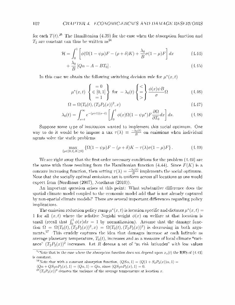
102 CHAPTER 4. ECONOMIC-EBCM'S AND DAMAGE RESERVOIRS
for each T (t).25 The Hamiltonian (4.39) for the case when the absorption function andT2 are constant can thus be written as26
H =
∫ 1
0
[φ(Ω(1− ψµ)F − (ρ+ δ)K) +
λ0
Bσ(1− µ)F
]dx (4.44)
+λ0
B[Qα− A−BT0] . (4.45)
In this case we obtain the following switching decision rule for µ∗(x, t)
µ∗(x, t)
= 0∈ [0, 1]
= 1
for − λ0(t)
<=>
φ(x)ψB
σΩ (4.46)
Ω = Ω(T0(t), (T2P2(x))2, x) (4.47)
λ0(t) =
∫ ∞s=t
e−(ρ+1)(s−t)[∫ 1
0
φ(x)Ω(1− ψµ∗)F ∂Ω
∂T0
dx
]ds. (4.48)
Suppose some type of institution wanted to implement this social optimum. Oneway to do it would be to impose a tax τ(λ) ≡ −λ0(t)
Bon emissions when individual
agents solve the static problems
maxµ∈[0,1],K≥0
Ω(1− ψµ)F − (ρ+ δ)K − τ(λ)σ(1− µ)F . (4.49)
We see right away that the rst order necessary conditions for the problem (4.49) arethe same with those resulting from the Hamiltonian function (4.44). Since F (K) is aconcave increasing function, then setting τ(λ) = −λ0(t)
Bimplements the social optimum.
Note that the socially optimal emissions tax is uniform across all locations as one wouldexpect from (Nordhaus (2007), Nordhaus (2010)).
An important question arises at this point: What substantive dierence does thespatial climate model coupled to the economic model add that is not already capturedby non-spatial climate models? There are several important dierences regarding policyimplications.
The emission reduction policy ramp µ∗(x, t) is location specic and dictates µ∗(x, t) =1 for all (x, t) where the relative Negishi weight φ(x) on welfare at that location issmall (recall that
∫ 1
0φ(x)dx = 1 by normalization). Assume that the damage func-
tion Ω = Ω(T0(t), (T2P2(x))2, x) = Ω(T0(t), (T2P2(x))2) is decreasing in both argu-ments.27 This crudely captures the idea that damages increase at each latitude asaverage planetary temperature, T0(t), increases and as a measure of local climate vari-ance (T2P2(x))2 increases. Let R denote a set of at risk latitudes with low values
25Note that in the case where the absorption function does not depend upon xs(t) the RHS of (4.43)is constant.
26Note that with a constant absorption function, 〈QSα, 1〉 = 〈Q(1 + S2P2(x))α, 1〉 =〈Qα+QS2αP2(x), 1〉 = 〈Qα, 1〉 = Qα, since 〈QS2αP2(x), 1〉 = 0.27(T2P2(x))2 denotes the variance of the average temperature at location x.

4.4. EBCM WITH DAMAGE RESERVOIRS 103
of Ω(T0(t), (T2P2(x))2), i.e. with high values of the arguments. The set R is a crudeattempt to capture latitudes that would be relatively most damaged by climate change.A plausible type of objective would be to solve the social problem above but withφ(x) > 0, x ∈ R, φ(x) ' 0, x /∈ R . We see right away that this social problem wouldrequire all xs not in R to reduce all emissions immediately. In general we have,
µ∗(x, t) = 1, for − λ0(t) >φ(x)ψB
σΩ (4.50)
and vice versa. This makes good economic sense. The marginal social burden onthe planet as a whole of a unit of emissions at date t, no matter from which x itemanates is, −λ0(t). Locations x where the Negishi weight on the location is small,where emissions per unit of output are relatively large (relatively large σ(x)), and thatare already relatively heavily damaged (Ω(T0(t), (T2P2(x))2, x) is high) are ordered tostop emitting. Thus our modeling allows plausible specications of the economic justiceargument stemming from geography to shape policy rules.
In the following section, we use this framework to extend our results in the presenceof an discontinuous absorption function that changes at the ice line. This is a morerealistic model which introduces ice line damages which we develop in the context of aDICE/RICE-type integrated assessment model.
4.4.2 Optimal mitigation in an IAM-type model with damage
reservoirs
We now introduce as the absorption function the version proposed in North (1975a)where
α(x, xs) = 1− α(x) =
α1 = 0.38x > xsα0 = 0.68x < xs
, (4.51)
where α(x) is the albedo. With this absorption function, the dynamics T0(t) in (4.34)and the T2 approximation in (4.43) become respectively
dT0
dt=
1
B
[−(A+BT0) +Q(α0 − α1)
∫ x=xs(t)
x=0
(1 + S2P2(x))dx+ E +Qα1
](4.52)
T2 =1
(1 + 6D)B
[5Q(α0 − α1)
∫ x=xs(t)
x=0
(1 + S2P2(x))P2(x)dx+Qα1S2
], (4.53)
where the equation for the ice line is, using (4.40),
xs(t) =
[2
3
Ts − T0(t)
T2
+1
3
] 12
. (4.54)
The objective (4.30) and the constraints (4.51)-(4.54) determine optimal mitigationover time and latitude. The discontinuous absorption function can create a strong non-linearity where a small change in T0 can cause a large change in damages at some lati-tudes. However this nonlinearity makes it dicult to proceed with analytical solutions.

104 CHAPTER 4. ECONOMIC-EBCM'S AND DAMAGE RESERVOIRS
To obtain a qualitative idea of the impact of the nonlinearity due to the absorptionfunction and the ice line, we use the climate parametrization used by North (1975a)(α0 = 0.68, α1 = 0.38, A = 201.4, B = 1.45, S2 = −0.483, Ts = −10, Q = 334.4). Theheat transport coecient D is found to be approximately 0.2214 by calibrating the iceline function to the current ice line estimate (xs = 0.95).28
The system (4.52)-(4.54) is highly nonlinear and can be simplied by deriving apolynomial approximation of xs as a function of T0(t). We proceed in the following way.If we substitute xs(t) from (4.54) into (4.53), then T2 is a xed point of (4.53). We solvenumerically the xed point problem (4.53) for values of T0 ∈
[−T0, T0
], obtaining the
solution T2(T0). Substituting this back into equation (4.54) gives us the xs(T2(T0), T0)which is then used to t a quadratic curve on (T0, xs) by using least squares. Thus xsis approximated by a convex curve xs = ζ0 + ζ1T0 + ζ2T
20 = ζ(T0), (ζ0, ζ1, ζ2) > 0.29
Making use of this approximation, the system (4.52)-(4.54) can thus be written as:
dT0
dt=
1
B[−(A+BT0) +Q(α0 − α1)θ(T0) + E +Qα1] (4.55)
where θ(T0) :=
[xs +
S2
2(x3
s − xs)]with xs := ζ0 + ζ1T0 + ζ2T
20
Assuming linear utility once again, the Hamiltonian can be written as:
H =
∫ 1
0
[φ[KβΩ(T0)(1− Λ)− (ρ+ δ)K] +
λ0
Bσ(1− µ)Kβ
]dx (4.56)
+λ0
B[−A−BT0 +Q(α0 − α1)θ(T0) +Qα1] .
We now assume that abatement costs are increasing in abatement activities, Λ = ψµ2.The optimal µ and K will thus be dened as:
µ∗(x, t) = − λ0σ
2BφψΩ(T0),∀x ∈ [0, 1] (4.57)
K∗(x, t) =
(ρ+ δ
β
) 1β−1[Ω(T0)(1− ψµ∗2)− λ0
φBσ(1− µ∗)
] −1β−1
. (4.58)
and the canonical system becomes:
dT0
dt=
[−A−BT0 +Q(α0 − α1)θ(T0) +
∫ 1
0
σ(1− µ∗)K∗βdx]
(4.59)
dλ0
dt= (ρ+ 1− Q
B(α0 − α1)θ′(T0))λ0 −
∫ 1
0
φ[K∗βΩ′(T0)(1− ψµ∗2)
]dx (4.60)
28The calibration procedure is explained in detail by North (1975b) (p.2035-2037).29The estimated quadratic function was
xs = 0.7126 + 0.0098T0 + 0.0003T 20 , R2 = 0.99.

4.4. EBCM WITH DAMAGE RESERVOIRS 105
which can be solved numerically given a specic shape of φ(x).To proceed further we need a more detailed specication for the damage function,
which as explained above should contain a temperature component denoted by D1(T0)and an ice line component, denoted by D2(T0). We specify the damage function inthe following way. Lost output from temperature induced damages is: Y − Y
1+D1(T0)=
Y D1(T0)1+D1(T0)
:= Y d1(T0). Lost output from ice line movement towards the poles written as a
function of T0 is: Y − Y1+D2(T0)
= Y D2(T0)1+D2(T0)
:= Y d2(T0). The sum of lost output from bothsources is: LostY = Y d1(T0) + Y d2(T0). Thus net output available for consumptionand mitigation is: Y − LostY = (1− d1(T0)− d2(T0))Y .
If we dene Ωi(T0) = 11+Di(T0)
, i = 1, 2, then the term (1 − d1(T0) − d2(T0)) can bewritten as the damage function Ω of the system (4.57)-(4.60) in the form
Ω(T0) = Ω1(T0) + Ω2(T0)− 1. (4.61)
As the global warming problem concerns damages resulting from temperature increasesrather than decreases, we restrict the state space to include only temperatures T0 >15C, i.e. in the vicinity of the present average global temperature level.30 In thespatial model used in this section, this temperature level is found by setting E = 0 andsolving (4.55), which gives us T0 ≈ 15.27. Hence, 15C can be viewed as a rough ballparkestimate of the preindustrial global temperature average. Damages are assumed to startat 15C and we thus write our normalized damage function as Ω(T0−15). Furthermore,we will use the same functional forms for the damage functions as used in section 4.3(see appendix 4.B).31
The EBCM that we presented in this section, resulting from the concepts developedin the earlier part of the paper, has many similarities to the traditional IAMs butalso two potentially important dierences. The rst is the discontinuous absorptionfunction and the second is an alternative shape for ice line damages as opposed to othertemperature related damages. Together they introduce complex nonlinearities into thetemperature dynamics. The question of whether these dierences imply signicantdeviations from the model's predictions, cannot be answered analytically due to thehigh complexity of the models. So we resort to numerical simulations.
Figure 4.2 shows the results for the spatial climate model presented in this section.As in section 4.2 this model also gives us 3 candidate optimal steady states, T01 <T02 < T03, where the largest and the smallest ones are saddles while the middle one isan unstable spiral.32 Between the unstable spiral T2 and the saddle T1 we have a Skiba
30During the development of many energy balance models in the 1960s and 1970s the main concernwas usually not that of global warming, but rather that of drastic global cooling that could resultdue to a slight decrease in the solar constant. This hypothesis was later coined Snowball earth byKirschvink (1992).
31The parameters estimates used in deriving gure 4.2 can be found in table 4.B in the appendix.32The corresponding eigenvalues are approximated numerically as e01 = [−0.7037, 0.7237], e02 =
[0.01± 0.3302i] and e03 = [−0.2355, 0.2555].

106 CHAPTER 4. ECONOMIC-EBCM'S AND DAMAGE RESERVOIRS
15 15.5 16 16.5 17 17.5 18 18.5 19−1
−0.9
−0.8
−0.7
−0.6
−0.5
−0.4
−0.3
−0.2
λ 0
solution path
T -isocline
λT -isocline
T02T01 T03 TnTs
Figure 4.2: Phase diagram for the system (4.59)-(4.60).
point Ts similar to that of section 4.2.33 Hence, dening the carbon tax as above i.e.τ = −λ0(t)/B, for low initial temperatures T00 < T1 a low but gradually increasingcarbon tax will be optimal, while for T1 < T00 < Ts the optimal carbon tax an invertedu-shape and is increasing close to Ts but starts decreasing as T1 is approached. In theregion Ts < T00 < T3 on the other hand optimal tax policy is u-shaped where initiallyin the vicinity of Ts it is optimal to levy a high carbon tax which then gradually willdecrease. Furthermore, gure 2 also depicts the case when ice line damages are omitted,Tn. In contrast to section 4.2, both of the isoclines are now aected and in order to keepthe gure from becoming too messy, we have chosen to plot only the single equilibriumat the crossing of these isoclines, which is denoted by the black dot at Tn in gure3. The qualitative behavior is however the same as in section 4.2, i.e. the damagereservoir - no ice line damage equilibrium is a saddle having a positive slope for theT -isocline and a negative slope for the λ-isocline.
33Greiner et al. (2009) nd multiple equilibria in a zero-dimensional EBCM, where albedo is modeledby a continuous s-shaped function of temperature. The derived multiple-equilibria and Skiba planeshowever, only apply for xed levels of abatement, i.e. there is just a single control variable (consump-tion). If, however, the social planner can control both consumption and abatement then there existsonly a single stable saddle. Our approach, apart from explicitly addressing the more appropriate one-dimensional model also diers in the sense that we obtain multiple equilibria and Skiba points whencontrolling both consumption and abatement.

4.5. THE DICE MODEL WITH DAMAGE RESERVOIRS 107
4.5 The DICE Model with Damage Reservoirs
Both the relatively simple model of section 4.2 and the more complex model of section4.4 strongly suggest that the explicit modeling of ice line damages shows the need forstrong mitigation now. In order to further demonstrate that this result is robust tothe choice of model, we now turn to the DICE model. The purpose of this exerciseis to show how the introduction of ice line damages into the damage function, alongthe lines suggested by the EBCMs, will aect the optimal emission policy impliedby DICE. The DICE model, probably the most well known of the IAMs, assumesthat all damages to the economy evolve according to the quadratic equation (A.5)in Nordhaus (2007). The calibrated version of this damage function is plotted onpage 51 of Nordhaus (2007). Based on this calibration we can see that a 4 degreewarming results in approximately a 5% loss of output. We proceed by calibrating ourdisaggregated damage function in the following way. First, in order to separate out theice line component from the total amount of damages, we follow the procedure shownin section 4.4.2. We thus replace (A.5) of Nordhaus (2007) with equation (4.61) fromsection 4.4.2. Hence, we have two separate damage components, D1(T ) and D2(T ),which can be calibrated independently. Next, we use the Nordhaus (2007) impactestimate of 5% loss of output for a 4 degree warming and make a rough assumptionthat exactly half of these damages should be attributed to the melting of ice sheetscausing sea level rises, ooding, changes in ocean currents, etc. Finally, using the sameshapes for the temperature and ice line specic components as in previous sections, i.e.D1(T ) = a1
2T 2 and D2(T ) = a2
T ξ
ϕ+T ξ, we proceed by calibrating the damage parameters
a1 and a2 so that D1(4) = D2(4) = 0.025. In this way our new damage functionproduces an amount of damage at a 4 degree warming which is equivalent to that ofthe original model but with diering damage estimates for other temperature levels.For D1(T ) this gives us an estimate of a1 = 0.0007813. In order to calibrate D2(T ) wehowever, also need to know the values of ξ and ϕ. The s-shaped function is usuallyused in models trying to capture thresholds or tipping points. Here, the parameters ξand ϕ will have an eect on the steepness and level at which temperature crosses such athreshold. We provide estimates for 3 dierent assumptions regarding these parametersin order to highlight how they impact on optimal trajectories.
Figure 4.3 plots the optimal emission control rate and carbon price resulting from theDICE-2007 model for three dierent sets of estimates for ξ and ϕ. First, for comparisonwe provide the trajectories for the original model without iceline damages i.e. a2 = 0,which are depicted as solid lines in both graphs. These trajectories are thus based onthe Nordhaus (2007) quadratic damage function calibrated as D(4) = 0.05 thus yieldinga 5% drop in output at a warming of 4 degrees. This provides a good benchmark forcomparison since both simulations with and without iceline specic damages in thisway yield the same damage estimate for a 4 degree rise in temperature.
As can be seen from this graph, the separation of dierent damage structures givesus u-shaped type policies where it is optimal to mitigate more initially as opposedto the normal gradualist policy ramp. Look rst at the dashed lines which depart
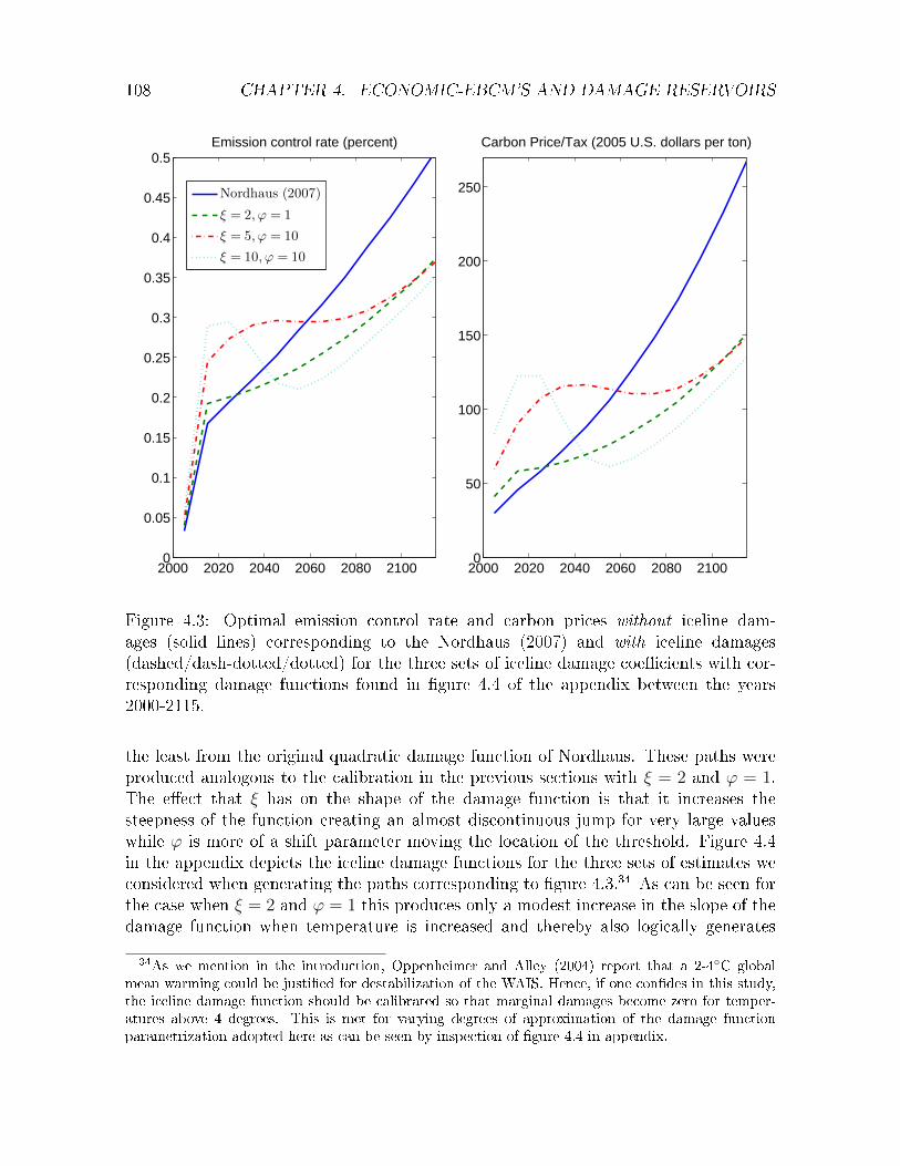
108 CHAPTER 4. ECONOMIC-EBCM'S AND DAMAGE RESERVOIRS
2000 2020 2040 2060 2080 21000
0.05
0.1
0.15
0.2
0.25
0.3
0.35
0.4
0.45
0.5Emission control rate (percent)
Nordhaus (2007)
ξ = 2, ϕ = 1
ξ = 5, ϕ = 10
ξ = 10, ϕ = 10
2000 2020 2040 2060 2080 21000
50
100
150
200
250
Carbon Price/Tax (2005 U.S. dollars per ton)
Figure 4.3: Optimal emission control rate and carbon prices without iceline dam-ages (solid lines) corresponding to the Nordhaus (2007) and with iceline damages(dashed/dash-dotted/dotted) for the three sets of iceline damage coecients with cor-responding damage functions found in gure 4.4 of the appendix between the years2000-2115.
the least from the original quadratic damage function of Nordhaus. These paths wereproduced analogous to the calibration in the previous sections with ξ = 2 and ϕ = 1.The eect that ξ has on the shape of the damage function is that it increases thesteepness of the function creating an almost discontinuous jump for very large valueswhile ϕ is more of a shift parameter moving the location of the threshold. Figure 4.4in the appendix depicts the iceline damage functions for the three sets of estimates weconsidered when generating the paths corresponding to gure 4.3.34 As can be seen forthe case when ξ = 2 and ϕ = 1 this produces only a modest increase in the slope of thedamage function when temperature is increased and thereby also logically generates
34As we mention in the introduction, Oppenheimer and Alley (2004) report that a 2-4C globalmean warming could be justied for destabilization of the WAIS. Hence, if one condes in this study,the iceline damage function should be calibrated so that marginal damages become zero for temper-atures above 4 degrees. This is met for varying degrees of approximation of the damage functionparametrization adopted here as can be seen by inspection of gure 4.4 in appendix.

4.6. SUMMARY, CONCLUSIONS, AND SUGGESTIONS FOR FUTURE RESEARCH109
paths similar to those of the original Nordhaus simulation. For higher values however,ξ = 5 and ϕ = 10, we begin to see an increasingly clear u-shape depicted by the dash-dotted lines in gure 4.3. The steepness of the iceline damage function thus seems to behave a large eect on the emission policy calling for more mitigation now. Finally, thedotted line depicts the most extreme case when ξ is raised to 10. As can be seen fromgure 4.4 in appendix this gives us a steep threshold type function for iceline damageswhere damages remain small up to a little over 1 degree and then increase rapidly. Thisproduces a clear u-shaped tax and emission policy as can be seen in gure 4.3.
The results above thus show o how a u-shaped policy might arise with heavy miti-gation now and less later when damages from climate change arrive in a more thresholdspecic manner as opposed to the more gradual increase, common in contemporarydamage functions. Although these results remain specic to our assumptions regardingthe shape of the damage function for the ice line as well as the temperature component,we still believe they are valuable since they show o the sensitivity of climate-economymodels to structural changes in the damage function.
4.6 Summary, Conclusions, and Suggestions for Future Research
In this paper we introduce the economics profession to spatial Energy Balance ClimateModels (EBCMs) and show how to couple them to economic models while derivinganalytical results of interest to economists and policy makers. While we believe thiscontribution is of importance in its own right, we also show how introduction of thespatial dimension incorporated into the EBCMs leads to new ways of looking at climatepolicy.
In particular, by accounting for an endogenous ice line and paying attention to theassociated damage reservoirs and albedo eects we show that due to nonlinearities evensimple economic-EBCMs generated multiple steady states and policy ramps which donot in general follow the gradualist predictions. These results carry over to morecomplex models where the economic module has an IAM structure. The interestingissue from the emergence of multiple steady states, is that when the endogenous ice lineand discontinuous albedo are ignored, as in traditional IAMs, the policy prescriptionof these models could be the opposite of the policy dictated by the economic-EBCMs.Furthermore the spatial aspect of the EBCMs allows arguments associated with thespatial structure of climate change damages to shape policy rules. When we appliedthe damage function implied by the EBCMs and calibrated appropriately simulationsin the DICE model gave results interpretable as a u-shaped policy ramp indicating animportant deviation from the gradualist policy ramp derived from the standard DICEmodel. Thus a rapid mitigation policy can be justied on the new insights obtained bycoupling the economy with the EBCMs.
Areas for further research could range from making the economics more sophisticatedby abandoning the simplifying assumption of linear utility; allowing for technical changeand knowledge spillovers across latitudes; or introducing strategic interactions amongregions and extensions of the EBCMs. It is thus also of importance to extend our Skiba

110 CHAPTER 4. ECONOMIC-EBCM'S AND DAMAGE RESERVOIRS
type analysis to include (exogenous) growth. This could give rise to a dynamic set ofSkiba points with a value function of both state and time, thus determining the optimalpolicy seperatly at each given point in time.35 Other extensions might also considerhow emissions arise more explicitly from the use of fossil fuels (see e.g. Golosov et al.(2011)). Future work also needs to be done regarding the extension of EBCMs to atwo-dimensional spherical EBCM, because Earth is a sphere, not a line. Brock andJudd (2010) are attempting to make a dent in this problem. They frame the problemas a recursive dynamic programming problem where the state vector includes a numberof spherical modes that are analogs of the modes in this paper as well as economicstate variables. Another possible extension could be the consideration of new policyinstruments. Emissions reduction acts on the outgoing radiation in the sense that byreducing emissions the outgoing radiation increases through the second term of theright hand side of (4.1). Another kind of policy could act on the rst term of the righthand side of (4.1) in the sense of reducing the incoming radiation. This type of policymight be associated with geoengineering options. Finally a policy which acts on thedamage function in the sense of reducing damages for any given level of temperatureand radiation balance might be associated with adaptations options. Unied economic-EBCMs might be a useful vehicle for analyzing the structure and the trade os amongthese dierent policy options.
35These extensions will undoubtedly increase the complexity and the computational needs for solvingthe economic-EBCMs.

References
Ackerman F., Stanton E.A., Decanio S.J., Goodstein E., Howarth R.B.,Norgaard R.B., Norman C.S. and Sheeran K.A., 2009, The Economics of350: The Benets and Costs of Climate Stabilization, Economics for Equity andEnvironment, pp. 150.
Agency E.E., 2010, The European environment - state and outlook 2010: synthesis,EEA, Copenhagen.
Brock W.A. and Judd K.L., 2010, Coupling Climate Models and Forward-LookingEconomic Models, in Abstract submitted to the Fall 2010 American Geophysical Unionmeeting in San Francisco (December 13-17) on "Climate Modeling in Support of Pol-icy Decision-making: Needs and Limitations, department of Economics, Universityof Wisconsin, Madison and Hoover Institution, Stanford University.
Brock W.A. and Starrett D., 2003, Managing Systems with Non-convex PositiveFeedback, Environmental and Resource Economics, vol. 26(4), pp. 575602.
Budyko M.I., 1969, The eect of solar radiation variations on the climate of the earth,Tellus, vol. 21, pp. 61119.
Carlson A.E., LeGrande A.N., Oppo D.W., Came R.E., Schmidt G.a.,Anslow F.S., Licciardi J.M. and Obbink E.a., 2008, Rapid early Holocenedeglaciation of the Laurentide ice sheet, Nature Geoscience, vol. 1(9), pp. 620624.
Golosov M., Hassler J., Krusell P. and Aleh T., 2011, Optimal taxes on fossilfuel in general equilibrium, Working Paper 17348, National Bureau of EconomicResearch.
Grass D., 2010, Numerical computation of the optimal vector eld in a shery model,Technical Report. ORCOS, Institute of Mathematical Methods in Economics, ViennaUniversity of Technology.
Grass D., Caulkins J.P., G. Feichtinger G., Gernot T. and Behrens D.A.,2008, Optimal Control of Nonlinear Processes: With Applications in Drugs, Corrup-tion, and Terror, Springer Verlag, Berlin.
Greiner A., Grüne L. and Semmler W., 2009, Growth and Climate Change:Threshold and Multiple Equilibria, SCEPA Working Paper 2009-7.
Hope C., 2006, The marginal impact of CO2 from PAGE2002: An integrated assess-ment model incorporating the IPCC's ve reasons for concern, Integrated AssessmentJournal, vol. 6(1), pp. 566577.
IPCC, 2001, Climate Change 2001: The Third Assessment Report of the Intergovern-mental Panel on Climate Change, Cambridge University Press, Cambridge.
111

112 CHAPTER 4. ECONOMIC-EBCM'S AND DAMAGE RESERVOIRS
IPCC, 2007, Climate Change 2007: The Fourth Assessment Report of the Intergovern-mental Panel on Climate Change, Cambridge University Press, Cambridge.
Judd K.L., 1998, Numerical Methods in Economics, vol. 2, MIT Press Books, TheMIT Press, 1 ed.
Judd K.L. and Lontzek T.S., 2011, Dynamic Stochastic General Equilibrium Analy-sis of Climate Change Policies, Conference presentation at INFORMS Annual Meet-ing - Austin, Texas.
Keller K., Bolker B.M. and Bradford D.F., 2004, Uncertain climate thresholdsand economic optimal growth, Journal of Environmental Economics and Manage-ment, vol. 48, pp. 723741.
Kerr R.A., 2008, Climate Tipping Points Come In From the Cold, Science, vol. 319,p. 153.
Kirschvink J., 1992, Late Proterozoic low-latitude global glaciation: the SnowballEarth, in W.J. Schopf and C. Klein, eds., The Proterozoic Biosphere: A Multidisci-plinary Study, chap. 2.3, Cambridge University Press.
Lempert R., Sanstad A. and Schlesinger M., 2006, Multiple equilibria in astochastic implementation of DICE with abrupt climate change, Energy Economics,vol. 28, p. 677689.
Lenton T.M., Held H., Kriegler E., Hall J.W., Lucht W., Rahmstorf S.and Schellnhuber H.J., 2008, Tipping elements in the Earth's climate system,Proceedings of the National Academy of Sciences of the United States of America,vol. 105, pp. 17861793.
Li X., Rowley R.J., Kostelnick J.C., Braaten D., Meisel J. and HulbuttaK., 2009, GIS Analysis of Global Impacts from Sea Level Rise, PhotogrammetricEngineering & Remote Sensing, vol. 75(7), pp. 80718.
Lindsay R.W. and Zhang J., 2005, The Thinning of Arctic Sea Ice, 1988−2003: HaveWe Passed a Tipping Point?, Journal of Climate, vol. 18, pp. 487994.
Lindzen R.S. and Choi Y.S., 2009, On the determination of climate feedbacks fromERBE data, Geophysical Research Letters, vol. 36(16), pp. 16.
Nævdal E., 2006, Dynamic optimisation in the presence of threshold eects when thelocation of the threshold is uncertain with an application to a possible disintegrationof the Western Antarctic Ice Sheet, Journal of Economic Dynamics and Control,vol. 30(7), pp. 113158.
Nordhaus W.D., 1994, Managing the Global Commons: the economics of the green-house eect, MIT Press, Cambridge, MA.

4.6. REFERENCES 113
Nordhaus W.D., 2007, A Question of Balance, Yale University Press, New Haven &London.
Nordhaus W.D., 2010, Economic aspects of global warming in a post-Copenhagenenvironment., Proceedings of the National Academy of Sciences of the United Statesof America, vol. 107(26), pp. 11721-26.
Nordhaus W.D., 2011, The architecture of climate economics: Designing a globalagreement on global warming, Bulletin of the Atomic Scientists, vol. 67(1), pp. 918.
Nordhaus W.D. and Boyer J., 2000, Warming the World: Economic Models ofGlobal Warming, MIT Press.
North G.R., 1975a, Analytical Solution to a Simple Climate Model with DiusiveHeat, Journal of Atmospheric Sciences, vol. 32, pp. 130107.
North G.R., 1975b, Theory of energy-balance climate models, Journal of AtmosphericSciences, vol. 32(11), pp. 203343.
North G.R., 1984, The small ice cap instability in diusive climate models, Journalof Atmospheric Sciences, vol. 41(23), pp. 339095.
North G.R., Cahalan R.F. and Coakley J.A., 1981, Energy Balance ClimateModels, Reviews of Geophysics and Space Physics, vol. 19(1), pp. 91121.
Oppenheimer M., 2005, Ice sheets, global warming, and Article 2 of the UNFCCC:An Editorial Essay, Climatic Change, vol. 68, pp. 25767.
Oppenheimer M. and Alley R.B., 2004, The West Antarctic Ice Sheet and LongTerm Climate Policy, Climatic Change, vol. 64(1/2), pp. 110.
Pierrehumbert R., 2011, Principles of planetary climate, Cambridge Univ Pr.
Roe G.H. and Baker M.B., 2010, Notes on a Catastrophe: A Feedback Analysis ofSnowball Earth, Journal of Climate, vol. 23(17), pp. 46944703.
Schaefer K., Zhang T., Bruhwiler L. and Barrett A., 2011, Amount andtiming of permafrost carbon release in response to climate warming, Tellus B.
Sellers W., 1969, A global climatic model based on the energy balance of the earth-atmosphere system, Journal of Applied Meteorology, vol. 8, pp. 392400.
Smith J.B., Schneider S.H., Oppenheimer M., Yohe G.W., Hare W., Mas-trandrea M.D., Patwardhan A., Burton I., Corfee-Morlot J., MagadzaC.H.D., Fussel H., Pittock a.B., Rahman A., Suarez A. and Van YperseleJ., 2009, Assessing dangerous climate change through an update of the Intergovern-mental Panel on Climate Change (IPCC) "reasons for concern", Proceedings of theNational Academy of Sciences, vol. 106, pp. 41334137.

114 CHAPTER 4. ECONOMIC-EBCM'S AND DAMAGE RESERVOIRS
Stanton E.A., 2010, Negishi welfare weights in integrated assessment models: themathematics of global inequality, Climatic Change, pp. 116.
Tarnocai C., Canadell J., Schuur E., Kuhry P., Mazhitova G. and ZimovS., 2009, Soil organic carbon pools in the northern circumpolar permafrost region,Global Biogeochemical Cycles, vol. 23(2), p. GB2023.
Tol R.S.J., 1997, On the optimal control of carbon dioxide emissions: an applicationof FUND, Environmental Modeling and Assessment, vol. 2, pp. 151163.
Trenberth K.E., Fasullo J.T., O'Dell C. andWong T., 2010, Relationships be-tween tropical sea surface temperature and top-of-atmosphere radiation, GeophysicalResearch Letters, vol. 37(3), pp. 15.
von Deimling T., Meinshausen M., Levermann A., Huber V., Frieler K.,Lawrence D. and Brovkin V., 2011, Estimating the permafrost-carbon feedbackon global warming, Biogeosciences Discussions, vol. 8.
Wang W.C. and Stone P.H., 1980, Eect of ice-albedo feedback on global sensitivityin a one-dimensional radiative-convective climate model, Journal of the AtmosphericSciences, vol. 37(5), pp. 54552.
Weitzman M.L., 2010, What Is The "Damages Function" For Global Warming? -and What Dierence Might It Make?, Climate Change Economics, pp. 5679.
Wu W. and North G.R., 2007, Thermal decay modes of a 2-D energy balance climatemodel, Tellus A, vol. 59(5), pp. 61826.
Xepapadeas A., 2005, Economic growth and the environment, in K.G. Mäler and J.R.Vincent, eds., Handbook of Environmental Economics, vol. 3, chap. 23, pp. 12191271,Elsevier.
Zhang T., Barry R., Knowles K., Ling F. and Armstrong R., 2003, Distri-bution of seasonally and perennially frozen ground in the northern hemisphere, inProceedings of the 8th International Conference on Permafrost, 21-25 July 2003,Zurich, Switzerland, pp. 12891294, AA Balkema, Lisse, the Netherlands.
Zimov S., Schuur E. and Chapin III F., 2006, Permafrost and the global carbonbudget, Science, vol. 312(5780), pp. 16121613.

4.A. APPENDIX 115
4.A Appendix: The two mode solution
In this appendix we show how to derive the two mode solution (4.8) - (4.11). We startwith the basic PDE
B∂T (x, t)
∂t= QS(x)α(x, xs)− [A+BT (x, t)− g(M(t))] (4.62)
+D∂
∂x
[(1− x2)B
∂T (x, t)
∂x
]The two mode solution is dened as:
T (x, t) = T0(t) + T2(t)P2(x), P2(x) =(3x2 − 1)
2(4.63)
then∂T (x, t)
∂t=dT0(t)
dt+dT2(t)
dtP2(x) (4.64)
∂T (x, t)
∂x= T2(t)
dP2(x)
dx= T2(t)3x (4.65)
Substitute the above derivatives into (4.62) to obtain:
BdT0(t)
dt+B
dT2(t)
dtP2(x) = QS(x)α(x, xs(t))−
[A+B(T0(t) + T2(t)P2(x))− g(M(t))] +D∂
∂x
[(1− x2)T2(t)3x
]or
BdT0(t)
dt+B
dT2(t)
dtP2(x) = QS(x)α(x, xs(t))− (4.66)
A−BT0(t)−BT2(t)P2(x)− g(M(t))− 6T2(t)P2(x)
Use: ∫ 1
0
Pn(x)Pm(x)dx = 〈Pn(x), Pm(x)〉 =δnm
2n+ 1(4.67)
δnm = 0 for n 6= m, δnm = 1 for n = 1
and note that P0(x) = 1, P2(x) = (3x2−1)2
Multiply (4.66) by P0(x) and integrate from 0 to 1 to obtain
BdT0(t)
dt= A−BT0(t) +
∫ 1
0
[QS(x)α(x, xs(t))] dx+ g(M(t)) (4.68)
Multiply (4.66) by P2(x) and integrate from 0 to 1 noting that∫ 1
0P2(x)dx = 0, and∫ 1
0P2(x)P2(x)dx = 1
5to obtain
BdT2(t)
dt= 5
∫ 1
0
[QS(x)α(x, xs(t))P2(x)] dx−BT2(t)− 6BDT2(t) (4.69)
where (4.68) and (4.69) are the ODEs of the two mode approximation given by (4.8) -(4.11).

116 CHAPTER 4. ECONOMIC-EBCM'S AND DAMAGE RESERVOIRS
4.B Appendix: analytics and calibration results for section 4.3
and 4.4
The production function in (4.24) is assumed to take the following form:
F (K −K2, h+ φK2) = (K −K2)β1(h+ φK2))β2 (4.70)
with β1 > 0, β2 > 0. The solution to problem (4.24) is derived from the rst orderconditions:
∂F
∂K= β1(K −K2)β1−1(h+ φK2))β2 − (δ + ρ) = 0 (4.71)
∂F
∂K2
= −β1(K −K2)β1−1(h+ φK2))β2 + β2φ(K −K2)β1(h+ φK2))β2−1 = 0 (4.72)
Solving the system (4.71) and (4.72) for K and K2 gives the solution to problem (4.24).
K∗2(h) =1
φ
((δ + ρ)
β1
(β1
φβ2
)1−β1) 1
β1−1+β2
− h
φ
K∗(h) =β1
φβ2
h+
(1 +
β1
β2
)K∗2(h)
Plugging these values back into (4.24) allows us to write π(h) as a linear function of h,i.e. π(h) = A+ Bh with
A :=
(β1
φβ2
)β1 ((δ + ρ)
β1
(β1
φβ2
)1−β1) β1+β2
β1−1+β2
− (δ + ρ)(1 + φ)
φ
((δ + ρ)
β1
(β1
φβ2
)1−β1) 1
β1−1+β2
B :=− (δ + ρ)
(β1
φβ2
− (1 + φ)
φ
)which is increasing in h given that β1/β2 < (1 +φ). Assuming also that D1(T ) = a1
2T 2,
D2(T ) = a2T ξ
ϕ+T ξand Ch(h) = chh
2. 36 Substituting this into (4.25), using the rstorder condition we can thus derive the function specic canonical system correspondingto (4.28)-(4.27) as:
dT
dt= aT − bTT + cT
B + λT cT2ch
, T (0) = T0 (4.73)
dλTdt
= (ρ+ bT )λT + a1T − 2a2e−2T (T − 1)T (4.74)
36The shape of D1(T ) has become fairly standard in the literature. Still, in a recent review byAckerman et al. (2009), they uncovered no rationale, whether empirical or theoretical, for adopting aquadratic form for the damage function. D2(T ) follows the s-shape found in e.g. Brock and Starrett(2003).
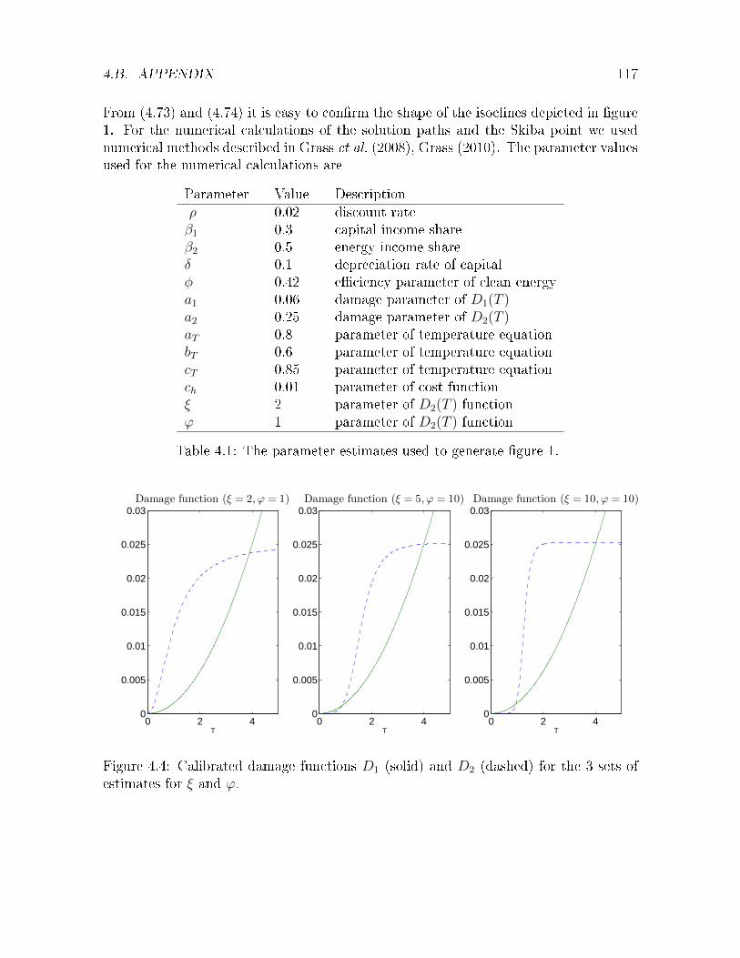
4.B. APPENDIX 117
From (4.73) and (4.74) it is easy to conrm the shape of the isoclines depicted in gure1. For the numerical calculations of the solution paths and the Skiba point we usednumerical methods described in Grass et al. (2008), Grass (2010). The parameter valuesused for the numerical calculations are
Parameter Value Descriptionρ 0.02 discount rateβ1 0.3 capital income shareβ2 0.5 energy income shareδ 0.1 depreciation rate of capitalφ 0.42 eciency parameter of clean energya1 0.06 damage parameter of D1(T )a2 0.25 damage parameter of D2(T )aT 0.8 parameter of temperature equationbT 0.6 parameter of temperature equationcT 0.85 parameter of temperature equationch 0.01 parameter of cost functionξ 2 parameter of D2(T ) functionϕ 1 parameter of D2(T ) function
Table 4.1: The parameter estimates used to generate gure 1.
0 2 40
0.005
0.01
0.015
0.02
0.025
0.03Damage function (ξ = 2, ϕ = 1)
T0 2 4
0
0.005
0.01
0.015
0.02
0.025
0.03Damage function (ξ = 5, ϕ = 10)
T0 2 4
0
0.005
0.01
0.015
0.02
0.025
0.03Damage function (ξ = 10, ϕ = 10)
T
Figure 4.4: Calibrated damage functions D1 (solid) and D2 (dashed) for the 3 sets ofestimates for ξ and ϕ.

118 CHAPTER 4. ECONOMIC-EBCM'S AND DAMAGE RESERVOIRS
Parameter Value Descriptionρ 0.02 discount rateA 201.4 capital income shareB 1.45 energy income shareα0 0.68 solar absorbation coecient for x < xsα1 0.38 solar absorbation coecient for x > xsζ1 0.7126 estimated coecient of iceline functionζ2 0.0098 estimated coecient of iceline functionζ3 0.0003 estimated coecient of iceline functionQ 334.4 incoming solar radiation divided by 4S2 -0.482 temperature distribution parameterσ 0.01 parameter of D2(T ) functionT0 15 parameter of D2(T ) functionδ 0.1 depreciation rate of capitalβ 0.5 capital income shareφ(x) 1 equal welfare weights for all xa1 0.002 damage function coecient functiona2 0.1 damage function coecient functionξ 2 parameter of D2(T ) functionϕ 1 parameter of D2(T ) function
Table 4.2: The parameter estimates used to generate gure 2.

Chapter 5
Assessing Sustainable Development in
a DICE World
5.1 Introduction
Integrated assessment models have become well used tools among researchers whentrying to estimate the costs associated with climate change (Cline, 1992; Nordhaus,1994; Manne et al., 1995; Hope, 2006). These general models describe the climate-economy inter linkages in terms of dynamic, global macroeconomic growth models thatare coupled with a climate model, describing the eects of increasing greenhouse gasconcentrations on temperature. The models typically assume rationality among eco-nomic agents and therefore take the normative approach of deriving optimal policiesfor the most ecient way of slowing climate change. This has resulted in varying rec-ommendations and much debate regarding the urgency for climate change mitigatione.g. ranging from postponing mitigation for several more decades (Nordhaus, 2007),to spending roughly 2% of GDP on mitigation eorts as proposed in the Stern Review(Stern, 2007). The debate surrounding these models have had large policy implications,one example being the worlds rst long term legally binding framework to tackle thedangers of climate change, known as the Climate Change Act 2008 1. As, these modelsare much referred to in the climate change debate it is troublesome that there is sucha divergence in modelling outcomes. The purpose of this paper is therefore to shedsome light on the matter by looking at what optimal consumption paths imply for thesocial-wellbeing of future generations and how these outcomes are aected by dierentpolicy regimes and the social-ethical assumptions undertaken. This is done by applyingthe concept of sustainable development to a neoclassical growth context.
Sustainable development is one of many ways in which we can compare social-wellbeing between dierent generations. The term became popular after a publicationby the World Commission on Environment and Development, which commonly became
1The Climate Change Act 2008 is a legislation forcing a 80% reduction in greenhouse gas emissionsin the UK by the year 2050. In the background documents several referrals are made to the Stern
Review. http://www.opsi.gov.uk/acts/acts2008/pdf/ukpga_20080027_en.pdf
119

120 CHAPTER 5. SUSTAINABLE DEVELOPMENT IN DICE
known as the Bruntland Commission Report. In this report sustainable developmentwas dened as "development that meets the needs of the present without compromisingthe ability of future generations to meet their own needs".2 Since then there have beenmany attempts to make this term operational in conventional theoretical models ofthe economy. Pezzey and Toman (2005) provide a good overview of some of thesedierent economic interpretations of sustainable development. In this paper I willdene sustainable development as non-declining social welfare. This denition relatesto the idea that each generation should leave behind at least as large a productive baseas they were given by their ancestors, meaning that each generation will have the samepossibility to generate welfare as the generation before them.3 The denition is mainlydue to Hamilton and Clemens (1999), Dasgupta and Mäler (2000) and Arrow et al.(2003) and is formulated in terms of the Ramsey-Koopmans social welfare functional,where a consumption path is denoted as sustainable if the time derivative of the socialwelfare functional is greater than or equal to zero.4 As emphasized in Arrow et al. (2003)the concept of optimality diers from sustainability. Even under an optimal policy planthe realized consumption path could be rendered unsustainable if for example the purerate of time preference, also commonly referred to as the utility discount rate, was settoo high.5 Therefore it is of interest to evaluate if the policy recommendations givenby the integrated assessment models also imply consumption paths that are consistentwith sustainable development i.e. that they do not exhaust the economy's productivebase. If this were the case, the policy recommendations given by the model would besteering us in a direction of impoverishment, without informing us that this was actuallyhappening.
This paper makes a rst pass at evaluating one of these integrated assessment modelin terms of sustainability, namely the DICE-2007 model (Nordhaus, 2007).6 The resultsshow that although the DICE-2007 model proves to be productive base sustainable, thisresult remains highly sensitive to the specic discounting assumptions employed withinthe model. When the discounting assumptions used in the DICE-2007 model are com-pared to the alternative discounting approach, of the DICE-(1994,1999) model, it isonly the former that manages to maintain a sustainable productive base. This ndingimplies that even though the parameters of the social welfare function are chosen con-sistently (i.e. to match historical rates of return on capital), with small implications forthe saving rate, the social cost of carbon or the optimal carbon tax, the relative choicesof these parameters still aect other aspects of the model. The robustness of these
2World Commission on Environment and Devolopement (1987)3The term productive base refers not only to all sorts of physical, human and natural capital, but
also to institutional arrangements and knowledge. Arrow et al. (2003) show that the maintenance ofa productive base implies and is implied by non-declining social welfare.
4The equivalent notion for the discrete time case, is that social welfare should be non-decliningbetween two periods of time.
5Arrow et al. (2003) also claim that it is possible to nd that along an optimum path social welfaredeclines for a period and then increases thereafter, in which case the optimum programme does notcorrespond to a sustainable path locally, but does so in the long run.
6DICE is an acronym for the "Dynamic Integrated model of Climate and the Economy".

5.1. INTRODUCTION 121
results are evaluated by introducing uncertainty regarding the most model sensitiveparameter values, which to a large extent shape the dynamic structure of the model.The conclusions from the uncertainty analysis is that the most important parameterestimates determining whether the model will turn out to be productive base sustainableor not, are the social welfare parameters (i.e. the utility discount rate and the elasticityof marginal utility) along with the total factor productivity (TFP) growth rate. Forexample, if the growth rate of TFP is set to zero, while leaving everything else un-changed, this would induce an unsustainable path in the DICE-2007 model. As arguedby Dasgupta et al. (1999) and recently shown in Vouvaki and Xepapadeas (2008b) thisassumption not implausible if natural capital is taken into account.
To my knowledge, this is the only study that has evaluated sustainability in terms ofchanging production possibilities within an integrated assessment model. Previous em-pirical analysis of productive base sustainability within theoretical frameworks includeVouvaki and Xepapadeas (2008a, 2009). Vouvaki and Xepapadeas (2008a) analyzethe behavior of the sustainability criterion by empirically parameterizing a standardSolow model subject to a ow pollutant (SO2) with estimates from the Greek econ-omy. In Vouvaki and Xepapadeas (2009) they instead evaluate sustainability in a globalmacroeconomic growth model subject to the inuence of a stock pollutant (CO2) for 44dierent countries. Their main empirical nding from the later paper is that a businessas usual increase in CO2 emissions will produce a negative measure of sustainability formost countries, while a constant level will yield a positive measure. Although, thereare many structural dierences between the model used in their analysis compared tothe DICE model, the results from this paper still indicates that the major dierencesin outcomes could be due to dierent assumptions regarding key parameter estimates.For example, when implementing the choices of social welfare parameters used by Vou-vaki and Xepapadeas (2009) in the DICE-2007 model, this produces an unsustainableproduction path.
The contribution of this paper is threefold. First, it shows how issues regarding sus-tainable development can be evaluated within an integrated assessment model frame-work. Second, it highlights which parameter estimates have the greatest eect on theevolution of the productive base. Third, it shows that model projections are sensitive tothe relative choices of social welfare parameters, regardless whether these are calibratedto match historical rates of return on capital.
The rest of this paper is structured as follows: Section 5.2 describes the basic struc-ture of the DICE-2007 model and how sustainable development can be evaluate withinthis framework. Section 5.3 presents result regarding sustainability for the dierentpolicy scenarios analyzed by Nordhaus (2007) and how these results are altered whenthe discounting assumptions of the DICE-(1994,1999) model are implemented. Section5.4 evaluates how uncertainty regarding key parameter estimates eect the results withrespect to sustainability. The nal section concludes.

122 CHAPTER 5. SUSTAINABLE DEVELOPMENT IN DICE
5.2 Sustainability Criterion in the DICE-model
The DICE model is one of the most accepted and widely known integrated assessmentmodels for analyzing links and feedbacks between economic and climatic system. TheDICE model was originally developed by Nordhaus (1994) and has since then beenupdated twice (Nordhaus and Boyer, 2000; Nordhaus, 2007); it is highly transparentand well documented with a freely available program code developed in the GAMSsoftware.7 The purpose of the model is to combine knowledge from economic andclimate sciences in order to derive insights into the costs and benets of alternativepolicies for slowing climate change.
5.2.1 DICE model structure
The model assumes that economic and climate policies should be constructed in a waythat maximizes the discounted population-weighted utility of per capita consumptionover a 600 year time period. This optimization problem is solved by choosing the levelof investment and emission control rate that maximizes the sum of discounted futureutility (see equation A.1 of appendix), subject to economic and climatic conditions(A.2-A.21).8 The model involves production of a single commodity, which can be usedfor either consumption or investment (A.7).
The aggregate output (A.3) of the model is produced using a Cobb-Douglas pro-duction function with an exogenous population growth (A.15) and Hicks-Neutral tech-nological change (A.16). The environmental damages and abatement costs (A.5-A.6)are assumed to be proportional to world output and the accumulation of capital (A.4),depends on investment decisions and the natural depreciation rate. The model in-corporates a simple carbon cycle system, where carbon ows between three adjacentreservoirs consisting of the atmosphere, upper and lower oceans. The accumulationof greenhouse gases in the atmosphere leads to a warming of the surface through anincrease in radiative forcing, which in turn leads to a rise in average global tempera-ture levels (A.9-A.14).9 The increase in global temperature levels results in physicaldamages that hinder future production possibilities e.g., through damages on agricul-ture, migration due to sea-level rise, adverse impacts on health, non-market damagesand potential catastrophic impacts. It is also assumed that damages from small andgradual temperature increases are low, but that damages rise in a non-linear fashion(A.5).
Output is produced using energy from either a carbon based or a non-carbon basedenergy source. Energy use produces an externality in form of CO2 emissions thattogether with the emissions from land use (A.19) change accumulates into the atmo-sphere (A.8-A.9) The amount of emissions originating from output depends on the level
7As of August, 2010, there also exist a newly updated beta version for Microsoft Excel. Due to lackof documentation for these models I have chosen to stick with the 2007 model.
8The level of investment Iτ and emission control rate µτ constitute the control variables of thisoptimization problem.
9Other greenhouse gases are also included in the model as exogenous trends in radiative forcing(A.21).

5.2. SUSTAINABILITY IN THE DICE-MODEL 123
of carbon-saving technological change, which is modelled as exogenous (A.17). Produc-tion decisions are also based on the size of the abatement costs, which depends on thecarbon-saving technology, the price of carbon-fuel replacements (backstop technology)(A.18) and the global participation rate in mitigation eorts (A.6).
The amount of available fossil fuels is limited, which implies that there is an upperbound on emission levels (A.20). This assumption generates hotelling or scarcity rentsfor carbon based energy sources that can be of use in describing the market path foremission reduction. This also implies that even in a laissez-faire economy there will besome amount of mitigation eort due to fossil fuel scarcity.
By modifying this general framework Nordhaus (2007) attempts to replicate andcompare alternative environmental policies for tackling climate change. In total, 16alternative policies are analyzed and compared with respect to the resulting economicand climatic outcomes that they produce.10
5.2.2 Sustainability
In order to evaluate whether the economic programmes analyzed within the DICE modelframework are consistent with sustainable development, I will use a similar criteria forassessing sustainable development as was adopted by Dasgupta and Mäler (2000).11 Asopposed to optimality, which focuses on achieving a maximum present value ow of con-sumption over time, the sustainability criterion instead aims at evaluating whether theproduction possibility set is growing or declining. The main advantage of this methodis that it can be incorporated into a general framework which is independent of whetherthe economies exhibit optimizing or non-optimizing behavior.12 In mathematical termsthe theory basically says that, a consumption path corresponds to a sustainable path attime t, if social welfare at time t+1 is not smaller than at time t, i.e. if V (t+1) ≥ V (t),where social welfare V (t) can be dened as in expression (A.1):13
V (t) =T∑τ=t
(1 + ρ)−(τ−t)U [c(τ)]L(τ) (5.1)
The value function V (t) reects social welfare as a function of a consumption andpopulation growth at each moment in time. Our consumption possibilities will furtherdepend on our production possibilities, which in turn is determined by our originalendowment of manufactured capital, human capital, natural capital and knowledge,and also by the institutions governing the economy. All these factors put together canbe said to constitute society's productive base (Dasgupta, 2001). If the institutional
10A brief description of these policies is given in section 3, for further details see Nordhaus (2007).11Dasgupta and Mäler (2000) developed their analysis in continuous time. Mäler (2001) provides a
translation of basic theory into a discrete time setting.12Dasgupta and Mäler (2000) dened a non-optimizing economy in the following way: a non-
optimizing economy is an economy where the government whether by design or incompetence doesnot choose policies that maximize intergenerational welfare.
13See also Dasgupta (2001).

124 CHAPTER 5. SUSTAINABLE DEVELOPMENT IN DICE
structure of the economy remains unchanged over time, the change in social welfarefrom one time period to the next, will be entirely determined by the changes in theproductive base. Under these circumstances sustainable development at time t can bedescribed as a pathway in which
V (Φ(t+ 1)) ≥ V (Φ(t)), at a given time t (5.2)
where Φ(t) denotes the state of the productive base at time t.14 As shown in Arrowet al. (2003), this implies that at each period in time t the change in social welfarewill equal genuine investment, which is dened as the accounting value of the rate ofchange in the productive assets of the economy. All assets which make up the economy'sproductive base will thus carry accounting prices, which are the weights determining, thedirection and magnitude, resulting from increases in specic productive assets, such asfor example manufactured capital, human capital, natural capital or technology. Thesustainability criterion will thus also be a measure of how the economy's wealth, interms of assets, are evolving.
5.2.3 Sustainability in the DICE model
Returning to the DICE model, a given set of parameter values, along with the emissioncontrol and saving rate associated with an optimal consumption path at time t and t+1,will imply that the value of the social welfare function V (t) will be entirely determinedby the state of its productive base. The productive base of the DICE model consistsof initial values for all variables that determine the state of the system at any givenmoment of time. The vector of elements included in the productive base of the DICE-model, are presented in Table 5.4 of the Appendix. These are the variables that, asopposed to the parameters and constants of the model, evolve over time and thereforeimplicitly determine the level of feasible consumption at each point in time. The DICEmodel runs over a time horizon of 600 years which is broken down into xed 10 yeartime intevals starting in 2005. Letting Φ(·) denote the vector of elements given in Table5.4, the sustainability criterion can thus be formulated as:
V (Φ(2015)) ≥ V (Φ(2005)) (5.3)
This means that sustainable development in the year 2005 is determined by the dif-ferences in the value of the sums of the maximized discounted future utility streamsevaluated in the years 2015 and 2005, respectively. This evaluation is done for twosets of estimates for the pure rate of time preference and elasticity of marginal utility,used in the DICE-2007 model (section 3) and the DICE-(1994,1999) model (section 4),respectively.
14It is also possible to formulate the much more demanding requirement for sustainable development,that this condition should be satised for all t.

5.3. SUSTAINABILITY OF POLICY SCENARIOS 125
5.3 Sustainability of policy scenarios and the role of the social
welfare parameters
One of the major novelties with the DICE-2007 model is that the social welfare functionhas been revised with updated values for the utility discount rate (ρ) and the elasticity ofmarginal utility (η). In the new model, the level of utility discounting has been revisedfrom an initial value of 3%, used in the DICE-(1994,1999) model to a lower value of1.5%, while simultaneously raising the value for the elasticity of marginal utility from 1(logarithmic) to a new value of 2. As explained in Nordhaus (2007): "this revision movesthe model closer to one that displays intergenerational neutrality while maintaining thecalibration of the models rate of return on capital with empirical estimates". Thisargument stems from the famous Ramsey Rule which states that along an ecient andoptimal economic programme the social rate of return on investment r will be given by:
r = ρ+ ηdc/dt
c(5.4)
With perfectly functioning capital markets, no taxes and lack of divergence betweenprivate and social benets, the social rate of return on investment will equal the privaterate, implying that the market interest rate (return on capital) can serve as an appro-priate proxy for social discounting.15 Hence, these two parameters work in dissimilarways; raising the value of η produces a more egalitarian outcome with increased inter-generational consumption smoothing while a lower value of ρ raises the value of futureconsumption streams. By recalibrating the model in this way Nordhaus nds a wayto lower the value for the pure rate of time preferences (thus pleasing his critics thathave pointed out the ethical dilemmas for high rates of utility discounting), while stillmaintaining the general model results.
5.3.1 General results
Table 1a presents sustainability measures based on criteria (5.3) for dierent policyscenarios and calibrations of the social welfare parameters ρ and η following the DICE-(1994,1999) and the DICE-2007 model where the policy scenarios are identical to theones analyzed by Nordhaus (2007). Table 1b shows the results of a separate run usingthe discounting assumptions following the Stern Review.16 The numbers in parenthesisare the exact sustainability measures dened in social welfare terms where a relativelyhigh (low) value is an indication of a higher (lower) level of sustainability. The num-bers proceeding these are index numbers indicating policy performance relative to thebusiness as usual (250-year delay) policy run. The rst column contains the socialwelfare parameters used in the 2007 model with a utility discount rate (ρ) of 1.5% anda elasticity of marginal utility (η) of 2. The second column contains the social welfareparameters used in the 1994 and 1999 versions of the model.
15See for example Arrow and Kurz (1970), Dasgupta and Heal (1979)16The dierences between this run and the last policy proposal in table 1a are explained in section
3.6.

126 CHAPTER 5. SUSTAINABLE DEVELOPMENT IN DICE
Table 1a: Sustainability criteria for alternative policy scenariosDiscounting assumptions DICE-2007 DICE-(1994,1999)
ρ = 1.5%, η = 2 ρ = 3%, η = 1Reference Scenarios250-year delay (BAU) 100 (21245) 100 (-107.14)50-year delay 100.22 (21292) 100.43 (-106.68Optimal 100.32 (21313) 100.66 (-106.43Kyoto ProtocolWith United States 100.11 (21269) 100.23 (-106.89)Without United States 100.02 (21249) 100.05 (-107.09)Strengthened 100.24 (21295) 100.21 (-106.92)Climatic constraintsConcentration limitsLimit to 1.5xCO2 92.06 (19559) 84.59 (-123.65)Limit to 2xCO2 100.23 (21294) 100.49 (-106.62)Limit to 2.5xCO2 100.32 (21313) 100.66 (-106.43)Temperature limitsLimit to 1.5C 97.23 (20656) 93.10 (-114.53)Limit to 2C 99.52 (21144) 98.77 (-108.46)Limit to 2.5C 100.14 (21275) 100.26 (-106.86)Limit to 3C 100.25 (21300) 100.59 (-106.51)
Ambitious proposalsGore Proposal 98.82 (20995) 94.81 (-112.7)Optimal (low-cost backstop) 101.92 (21653) 104.76 (-102.04)Stern Proposal (dual-discount)* 101.98 (21453) (98.92) -108.22
*See section 3.6 for details.
Table 1b: Sustainability criteria for the Stern Reviewρ = 0.1%, η = 1
Stern Review 1731
An immediate observation from table 1a is that all alternative policy scenarios ana-lyzed in the 2007 model (column 1) have large positive sustainability measures whilethe social welfare parameters associated with the 1994 and 1999 model (column 2) gen-erate negative sustainability measures. This is an interesting result which indicates thatthe choices of these two key parameter estimates are very important in determining themodel outcome with respect to sustainability and that a calibration approach whichonly focuses on maintaining a certain level of return on capital does not insure againstpossibly large impacts on the economy´s productive base. Further, as will be shownin the sensitivity analysis, the sustainability measure is more sensitive to the choice ofelasticity of marginal utility compared to the utility discount rate.
5.3.2 Reference scenarios
The rst policy run analyzed is one where governments take no policy measures tointernalize the costs of damages associated with greenhouse warming. In this policyrun the market path for allocating carbon fuels is followed for 250 years, after which

5.3. SUSTAINABILITY OF POLICY SCENARIOS 127
the world wakes up and optimizes its emission trajectory in light of climate damages.17
This run corresponds to the business as usual (BAU) scenario which is also referred toas the baseline or no controls case. The baseline scenario can be compared to the opti-mal policy scenario where an optimal path for emission reduction is followed in order tomaximize the value of net economic consumption. Comparing the sustainability mea-sures of these two we nd that the optimal policy scenario produces a more sustainableconsumption path in both columns. This is inline with what we would expect sincean optimal policy run corresponds to the case where the best possible policy path isfollowed with regards to the economic, technological and geophysical constraints for theentire time horizon. Logically this should improve on the case where the market pathis followed for 250 years with no consideration for damages inicted by climate change.The reason for this is that when the market path is followed, one of the control variables(the emission control rate) is xed, which leads to an inferior solution implying thatthe optimal run is more sustainable. The same is true to that of the 50-year delay runwhich is equivalent to the 250-year delay except that the world wakes up earlier, whichimplies that it lies closer to the projections of the optimal policy run.
5.3.3 Kyoto Protocol
Concerning the three versions of the Kyoto Protocol runs they all produce sustainableresults which supersede that of BAU. This is because the emission control rate chosen inthis run corresponds better to that of the optimal policy run. We can also see that theversion with the United States included generates a higher sustainability measure thanthe one without. This is a logical result indicating that a higher world participationrate in climate policies is more eective and hence increases sustainability. In thestrengthened version of the protocol more countries are added gradually; they beginwith a 10 percent emission reduction and reduce further with 10 percent every 25years, which generates a more sustainable path than the other versions of the protocol.However, as can be seen in column 2 the equivalent result does not hold for the socialwelfare parameters used in the DICE-(1994,199) model. It is dicult to assess the exactreasons for this, but the result in itself shows that the choice of time discounting andelasticity of marginal utility will matter when comparing dierent policy scenarios.
5.3.4 Climatic thresholds
The next two policy categories impose dierent concentration and temperature limitconstraints which comply to quantitative regulation forms such as quotas, targets orcommands. Computationally, these are similar to the optimal run but with an upperlimit climate constraint imposed. The rst is an upper atmospheric CO2-concentrationlevel constraint which is set in relation to preindustrial levels. The second is an upperlimit on global temperature increase compared to 1900 levels. The economic intuition
17The market path implies that the optimal consumption path is chosen without consideration forthe externalities associated with production. A more detailed description of the policy runs can befound in Nordhaus (2007), the time period 250 years is arbitrary and chosen for computational reasons,for example increasing the time span to 350 years has a very marginal eect.

128 CHAPTER 5. SUSTAINABLE DEVELOPMENT IN DICE
behind these upper limit constraints is to consider them as threshold levels after whichdamages become innitely large. For both of these constraints we see that as the limitsbecome increasingly generous, the sustainability increase in both columns. This patternmay at rst glance seem counterintuitive, but is simply a consequence of modellingassumptions. The likely reason for this behavior is that the production possibility setwill become increasingly limited as the emissions associated with production must beconstrained to correspond with stricter upper limit climate constraints. Hence, thecosts of the restrains on capital gains resulting from stricter climate constraints seem tooutweigh the benets associated with reduced damages from global warming. However,compared to the BAU scenario the upper limits of 2×CO2-concentration levels and 2.5-temperature rise produce more sustainable results for both columns. The restrictionsimposed are all binding in the optimization problem except in the case of 2.5 × CO2-concentration level which therefore takes on the same value as in the optimal policyrun.
5.3.5 Ambitious proposals
The last three policy runs constitute ambitious proposals which call for sharp emissionreductions.
The Gore proposal run implies a rise in the emission control rate from 15 percentin 2010 to 90 percent in 2050, further it is assumed that participation increases froman initial 50 percent to a 100 percent by 2050. This policy run does not improvesustainability compared to BAU regardless of the choice of social welfare parameters.The reason for this is that with these climatic constraint policies, a high emission controlrate reduces production possibilities to a greater extent than the benets received fromdamage reduction.
The Optimal (low-cost backstop) policy analyzes the implications of the developmentof a new energy source that could replace fossil fuels at a cost that is competitive withtoday's technologies. This scenario corresponds to the optimal run except that theprice for the backstop technology is reduced, which in turn lowers abatement costs.This means that more abatement can be done for the same amount of money; leadingto a higher sustainabilty measure.
5.3.6 The Stern Review
In order to assess the results of applying the discounting assumptions adopted in theStern Review Nordhaus uses, what he terms a dual-discounting approach. Here theemission control rates corresponding to the discounting assumptions used in the SternReview are set as constraints on the Optimal policy scenario using the discountingassumptions of the DICE-2007 model. The reason for carrying out this exercise is thata meaningful comparison of policy scenarios requires that social preference structuresare the same.
Even though compelling, I nd a certain awkwardness to this approach. In thesimulation run Nordhaus takes market preferences to be the correct proxy for socialpreferences. He then tries to assess the impacts of forcing emission standards corre-

5.4. SENSITIVITY ANALYSIS 129
sponding to governmental preferences upon this society. However, if a government,discounting in a Stern like fashion, were to adopt an optimal emission control rate theoptimal emission path would be optimal only conditional upon the corresponding opti-mal savings rate. This is also captured in the DICE model since governments choice ofemission control rate is intertwined with its choice of saving rate. In sum, the sustain-ability measure becomes dicult to interpret. However for sake of completeness theresult of this policy run is presented in the last row of table 1a.
The results of a policy scenario adopting the simple discounting assumptions of theStern Review is presented in table 1b. This policy run corresponds to the Optimal runin table 1a but with a utility discount rate of 0.1% and a elasticity of marginal utilityof 1. This results in a sustainability measure of approximately 1731 units of socialwelfare. As previously pointed out this measure is not directly comparable to that oftable 1a since dierent preference structures are applied. However, it can be notedthat a lower utility discount rate implies that future well-being is valued higher, whilea lower elasticity of marginal utility implies that present value of a marginal increasein consumption will rise compared to an equivalent marginal increase in the future.Therefore, as indicated by the relatively lower estimate of sustainability, the eect oflowering the elasticity of marginal utility seems to dominate the sustainability impactof a decrease in the utility discount rate.
5.4 Sensitivity analysis
As was shown in the previous section, the projections of sustainability within the DICE-model rely heavily upon the assumptions made regarding the estimates of social wel-fare parameters. The other parameter estimates are based on statistical analysis andscientic predictions regarding the evolution the relevant climatic and socioeconomicvariables. Usual problems of incomplete knowledge regarding for example measurementand structural issues generate uncertainty. In this section I will address uncertainty re-garding the estimated values for some of the key parameter estimates. I will restrictthe analysis to the business as usual policy scenario and optimal policy scenarios.18 Iwill further use the basic references regarding parameter uncertainty provided by Nord-haus (2007) with just a few exceptions. Nordhaus selected eight major parametersof uncertainty, including: the growth rate of total factor productivity, the rate of de-carbonization, temperature sensitivity with regard to a doubling of CO2-concentrationlevels, damage to output from greenhouse warming, the cost of a backstop technology,population growth, the atmospheric retention fraction of CO2, and the total availabilityof fossil fuels.19 To this list, which is presented in Table 5.1, I have also added uncer-tainty regarding the choice of utility discount rate and elasticity of marginal utility. Ihave chosen a normal distribution for both these model parameters, with an expected
18Uncertainty has also been addressed within other policy scenarios. These simulations have led tosimilar conclusions to that of the BAU scenario and are therefore left out.
19In Nordhaus (2007) a technical background is given regarding the estimation processes underlyingsome of the most model-sensitive parameters.

130 CHAPTER 5. SUSTAINABLE DEVELOPMENT IN DICE
value of 1.5% and a standard deviation of 0.4% for the utility discount rate and an ex-pected value of 2 and a standard deviation of 0.15 for the elasticity of marginal utility.20
This means that roughly 99.7% of all parameter draws fall in the range [0.3, 2.7] for theutility discount rate and in the range [1.55, 2.45] for the elasticity of marginal utility.21
Further, I assume that future utility is valued less than current utility and thereforediscard all negative values for the utility discount rate. Considering, asymptotic pop-ulation, this parameter is also drawn from the normal distribution. All values drawnabove or below four standard deviations from the mean are discarded. This impliesthat world population will never decline below 1850 year levels. All other estimateswith exception for the temperature sensitivity parameter are drawn from the normalprobability distributions with means and variances provided in Table 5.1.
Table 5.1: Uncertainty regarding specic parameter assumptions.Parameter Denition Mean S.D.ρ Pure rate of time preference (time discount rate) 0.015* 0.004η Elasticity of marginal utility 2.0* 0.15ga Growth rate of total factor productivity 0.092 0.04gσ Growth rate of CO2-emission to output ratio -0.073 0.02T2× CO2 Temperature sensitivity (°C) to CO2 doubling 3.06 1.01π2 Damage parameter 0.0028 0.0013Pback Cost of backstop technology ($) 1170 468PopAsym Asymptotic global population 8600 1892CarCyc Transfer coecient in carbon cycle 0.189 0.017Fosslim Total amount fossil fuels (Billion tons of carbon) 6000 1200
*The monte-carlo analysis of section 4.3 uses mean values of 3% and 1 respectively for the
simulations of the DICE-(1994,1999) model.
The eect on atmospheric temperature associated with a doubling of CO2 (T2 ×CO2) is set to 3 in the DICE-model, however many estimates from models and obser-vations yield broad and asymmetric probability distributions. Roe and Baker (2007)derive a theoretical probability distribution for temperature sensitivity which, in a satis-factory way manages to approximate, several other published probability distributionsusing a simple system of linear physical feedback processes. I model uncertainty re-garding temperature sensitivity using the theoretical probability distribution derivedin their article. Inline with an example from this article, I assume a normal feedbackdistribution with a mean and a standard deviation of 0.1 and leave out upper tail valuesexceeding three standard deviations in order to avoid catastrophic runaway feedbackeects. This means that 99.9% of the temperature sensitivity values will fall in the
20Expected values of 3% and 1 where used for the DICE-94 simulation in section 4.321The utility discount rate was set as large as possible without risking the possibility of drawing
negative values in the monte carlo simulation conducted in section 4.3. Concerning the elasticityof marginal utility the GAMS software had problems solving the model for values above 2.7 so thestandard deviation was set in order to not risk that values above 2.7 were drawn.
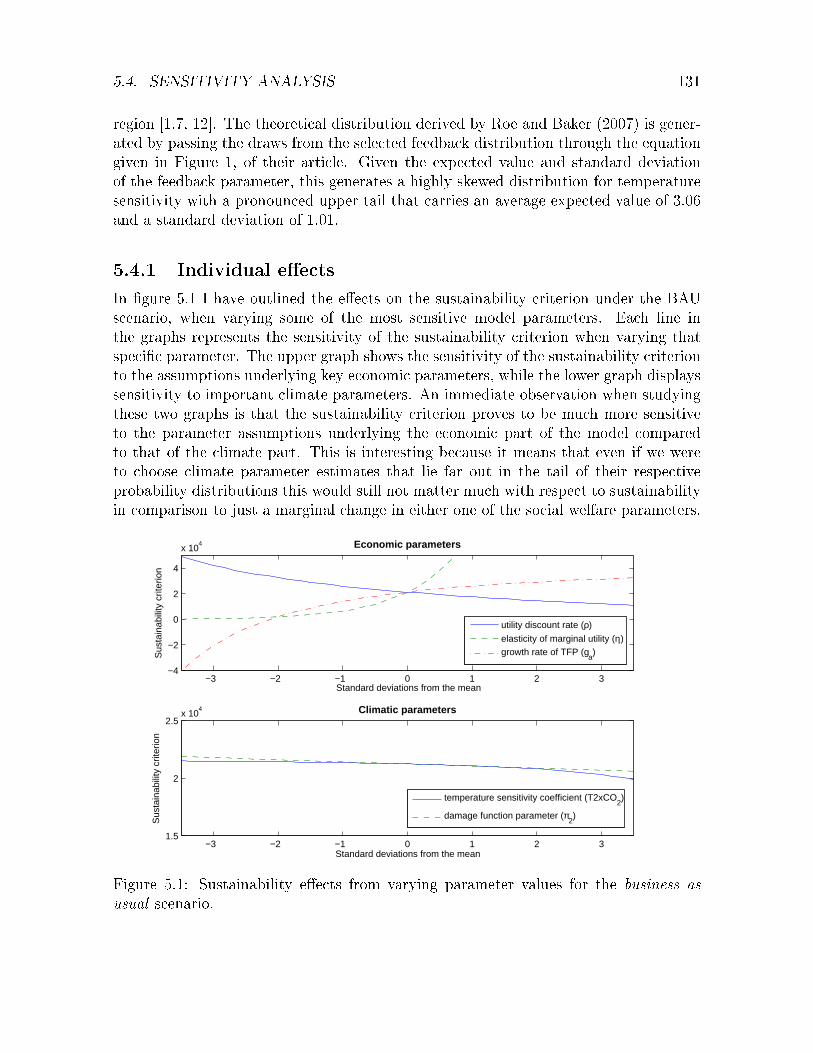
5.4. SENSITIVITY ANALYSIS 131
region [1.7, 12]. The theoretical distribution derived by Roe and Baker (2007) is gener-ated by passing the draws from the selected feedback distribution through the equationgiven in Figure 1, of their article. Given the expected value and standard deviationof the feedback parameter, this generates a highly skewed distribution for temperaturesensitivity with a pronounced upper tail that carries an average expected value of 3.06and a standard deviation of 1.01.
5.4.1 Individual eects
In gure 5.1 I have outlined the eects on the sustainability criterion under the BAUscenario, when varying some of the most sensitive model parameters. Each line inthe graphs represents the sensitivity of the sustainability criterion when varying thatspecic parameter. The upper graph shows the sensitivity of the sustainability criterionto the assumptions underlying key economic parameters, while the lower graph displayssensitivity to important climate parameters. An immediate observation when studyingthese two graphs is that the sustainability criterion proves to be much more sensitiveto the parameter assumptions underlying the economic part of the model comparedto that of the climate part. This is interesting because it means that even if we wereto choose climate parameter estimates that lie far out in the tail of their respectiveprobability distributions this would still not matter much with respect to sustainabilityin comparison to just a marginal change in either one of the social welfare parameters.
−3 −2 −1 0 1 2 3−4
−2
0
2
4
x 104
Standard deviations from the mean
Sus
tain
abili
ty c
riter
ion
Economic parameters
utility discount rate (ρ)
elasticity of marginal utility (η)growth rate of TFP (g
a)
−3 −2 −1 0 1 2 31.5
2
2.5x 10
4
Standard deviations from the mean
Sus
tain
abili
ty c
riter
ion
Climatic parameters
temperature sensitivity coefficient (T2xCO2)
damage function parameter (π2)
Figure 5.1: Sustainability eects from varying parameter values for the business asusual scenario.

132 CHAPTER 5. SUSTAINABLE DEVELOPMENT IN DICE
From the upper graph we can further see that the elasticity of marginal utility hasthe largest impact on sustainability in the sense that the variation in the sustainabilitycriterion is the largest for this variable.22 The sustainability criterion increases expo-nentially as this estimate increases in value. Although not shown in the gure, valuesbelow 0.9 for this parameter will generate negative values for the sustainability criterion.
As previously mentioned we cannot compare the sustainability measure for dierentvalues of η, in the sense of saying that one is more sustainable than the other. Thereason for this is that social welfare is being measured using a cardinal utility functionwhere preferences are assumed to be identical among all individuals. By denition thisutility function allows only for ranking of dierent consumption bundles conditionalon the assumed preference structure. For the exact same reason the denition of sus-tainability used in this paper, has to be conditioned on the assumed social preferencesand cannot be compared to other potential societies having dierent preferences. How-ever, the sensitivity analysis points out the importance of choosing the estimate of ηwith great care since the selection can greatly alter the model outcome with respect tosustainability.
The growth rate of total factor productivity is the second most model sensitiveparameter. Judging from the variation in this parameter, the model becomes unsus-tainable at about -2 standard deviations from the mean, i.e. the model has about a2.5% probability of becoming unsustainable, cetris paribus. The utility discount rate isthe third most model sensitive parameter. The sustainability criterion increases in anexponential fashion when the utility discount rate approaches zero and declines slowlywhen the discount rate increases. The model becomes unsustainable rst when theutility discount rate is roughly 6.2% i.e at about 12 standard deviations from the mean.This means that if the model predictions were to hold with certainty we could allowourself to discount at a rate as high as 6.2% before the productive base we leave behindis smaller than the one we started with.
5.4.2 Synergistic eects
Although the above analysis provides an indication of how each specic parametervalue eects the sustainability criterion, it does not capture the possibility of interact-ing eects amongst them. The histograms in gure 5.2 shows the empirical probabilitydistributions of the sustainability criterion, for the BAU scenario under the two dif-ferent discounting assumptions used in the DICE-(1994,1999) and DICE-2007 model.23
The results were generated in a Monte Carlo simulation based on 10000 draws using theuncertainty assumptions depicted in table 5.1. The model was thus optimized 10000times for each set of parameter estimates that were randomly drawn from their respec-tive probability distributions. By recording the sustainability criterion for each set ofparameter estimates the empirical probability distributions depicted in gure 5.2 were
22That is the dierence in sustainability values attained at 3.5 and -3.5 standard deviations fromthe mean.
23The mean values for ρ and η in table 5.1 were thus set to correspond to the DICE-(1994,1999)model.
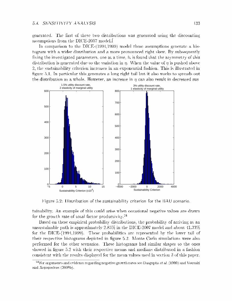
5.4. SENSITIVITY ANALYSIS 133
generated. The rst of these two distributions was generated using the discountingassumptions from the DICE-2007 model.¨
In comparison to the DICE-(1994,1999) model these assumptions generate a his-togram with a wider distribution and a more pronounced right skew. By subsequentlyxing the investigated parameters, one at a time, It is found that the asymmetry of thisdistribution is generated due to the variation in η. When the value of η is pushed above2, the sustainability criterion increases in an exponential fashion. This is illustrated ingure 5.1. In particular this generates a long right tail but it also works to spreads outthe distribution as a whole. However, an increase in η can also result in decreased sus-
−4000 −2000 0 2000 40000
100
200
300
400
500
600
700
800
3% utility discount rate, 1 elasticity of marginal utility
Sustainability Criterion−5 0 5 10 150
100
200
300
400
500
600
1.5% utility discount rate, 2 elasticity of marginal utility
Sustainability Criterion (x104)
Figure 5.2: Distribution of the sustainability criterion for the BAU scenario.
tainability. An example of this could arise when occasional negative values are drawnfor the growth rate of total factor productivity.24
Based on these empirical probability distributions, the probability of arriving at anunsustainable path is approximately 2.85% in the DICE-2007 model and about 41.33%for the DICE-(1994,1999). These probabilities are represented by the lower tail oftheir respective histograms depicted in gure 5.2. Monte Carlo simulations were alsoperformed for the other scenarios. These histograms had similar shapes to the onesshowed in gure 5.2 with their respective means and medians distributed in a fashionconsistent with the results displayed for the mean values used in section 3 of this paper.
24For arguments and evidence regarding negative growth rates see Dasgupta et al. (1999) and Vouvakiand Xepapadeas (2008b).
134 CHAPTER 5. SUSTAINABLE DEVELOPMENT IN DICE
5.5 Conclusions
This paper explores how sustainable development in terms of society's future produc-tion possibilities can be analyzed within an integrated assessment model of climatechange. The study shows that the DICE-2007 model is production base sustainable inits current form but that the degree of sustainability is highly dependent on the valuesof key parameter estimates. When revising the social welfare function using estimatesfor the utility discount rate and elasticity of marginal utility originally put forth in theDICE-(1994,1999) model, this results in an unsustainable productive base. This nd-ing implies when evaluating production base sustainability as dened in this article, theconclusions might dier vastly depending on how the parameters of the social welfarefunction are chosen. It is not enough to calibrate to an assumed rate of return oncapital since sustainability is aected dierently depending on the choice of elasticity ofmarginal utility and discount rate even when the dierent choices lead to the same rateof return on capital via the Ramsey rule. Instead it might be better to calibrate themindependently, considering each parameter estimates individual eect on social welfare.Further, when assessing uncertainty regarding parameter estimates it is found that totalfactor productivity growth along with the social welfare parameters are those that tothe greatest extent inuence whether or not the model will maintain a sustainable pro-ductive base. This analysis shows that the economic parameters completely dominateimportant climatic parameters such as the damage parameter or temperature sensitiv-ity coecient, in the sense that small incremental changes in the economic parametershave a much larger eect on sustainability than corresponding large changes in theclimatic parameters. Even when very extreme estimates are assumed for the climatechange parameters, this still does not eect the model outcome w.r.t. sustainabilityas much as a slight reduction in the utility discount rate would have. The sensitivityof the model with respect to the social welfare parameters calls for careful evaluationsof the projections and that before using it for policy recommendation purposes it isimportant to highlight these aspects to policy makers.

References
Arrow K., Dasgupta P. and Mäler K.G., 2003, Evaluating Projects and Assess-ing Sustainable Development in Imperfect Economies, Environmental and ResourceEconomics, vol. 26(4), pp. 647685.
Arrow K.J. and Kurz M., 1970, Public Investment, the Rate of Return and OptimalFiscal Policy, John Hopkins University Press, Baltimore.
Cline W., 1992, The Economics of Global Warming, Institute for International Eco-nomics, Washington, DC.
Dasgupta P., 2001, Human Well-Being and the Natural Environment, Oxford Uni-versity Press, Oxford.
Dasgupta P. and Heal G., 1979, Economic Theory and Exhaustible Resources, Cam-bridge Universdity Press, Cambridge, UK.
Dasgupta P. and Mäler K.G., 2000, Net national product, wealth, and social well-being, Environment and Development Economics, vol. 5(01), pp. 6993.
Dasgupta P., Mäler K.G. and Barrett S., 1999, Intergenerational Equity, SocialDiscount Rates, and Global Warming., in P. Portney and J. Weyant, eds., Discountingand Intergenerational Equity, pp. 5177, Resources for the Future., Washington, D.C.
Hamilton K. and Clemens M., 1999, Genuine savings rates in developing countries,World Bank Economic Review, vol. 13(2), pp. 33356.
Hope C., 2006, The social cost of carbon: What does it actually depend on?, ClimatePolicy, vol. 6(5), pp. 566577.
Mäler K.G., 2001, Wealth and Well-being in a Model With Discrete Time, DiscussionPaper Series No.146, The Beijer Institute of Ecological Economics.
Manne A.,Mendelsohn R. andRichels R., 1995, MERGE : A model for evaluatingregional and global eects of GHG reduction policies, Energy Policy, vol. 23(1), pp.1734.
Nordhaus W. and Boyer J., 2000, Warming the World: Economic Models of GlobalWarming, MIT Press.
Nordhaus W.D., 1994, Managing the Global Commons: the economics of the green-house eect, MIT Press, Cambridge, MA.
Nordhaus W.D., 2007, A Question of Balance: Weighing the Options on GlobalWarming Policies.
135

136 CHAPTER 5. SUSTAINABLE DEVELOPMENT IN DICE
Pezzey J.C. and Toman M.A., 2005, Sustainability and its economic interpretations,in M.T. R.D. Simpson and R. Ayres, eds., Scarcity and Growth: Natural Resourcesand the Environment in the New Millennium, pp. 121141, RFF Press, Washington,D.C.
Roe G.H. and Baker M.B., 2007, Why is climate sensitivity so unpredictable?, Sci-ence, pp. 629632.
Stern N., 2007, The economics of climate change: The stern review., cambridge Uni-versity Press, Cambridge.
Vouvaki D. and Xepapadeas A., 2008a, Changes in social welfare and sustainability:Theoretical issues and empirical evidence, Ecological Economics, vol. 67(3), pp. 473484.
Vouvaki D. and Xepapadeas A., 2008b, Total Factor Productivity Growth whenFactors of Production Generate Environmental Externalities, MPRA Paper 10237,University Library of Munich, Germany.
Vouvaki D. andXepapadeas A., 2009, Productive Base Sustainability under ClimateChange: Theoretical Results and Empirical Evidence, Economics: The Open-Access,Open-Assessment E-Journal, vol. 3(2009-11).
World Commission on Environment and Devolopement, 1987, Our commonfuture, oxford University Press, Oxford, ISBN 0-19-282080-X.

5.A. APPENDIX 137
5.A Appendix
Table 5.2: Endogenous relationships(A.1) V (t) =
∑Tτ=t(1 + ρ)−(τ−t)U [c(τ)]L(τ)
(A.2) U [c(τ)] = c(τ)(1−η)/(1− η), c(τ) = C(τ)/L(τ)(A.3) Q(τ) = Ω(τ)[1− Λ(τ)]A(τ)K(τ)γL(τ)(1−γ)
(A.4) K(τ + 1) = K(τ)(1− δ)10 + 10I(t)(A.5) Ω(τ) = 1/[1 + π1TAT (τ) + π2TAT (τ)2](A.6) Λ(τ) = π(τ)θ1(τ)µ(τ)θ2 , π(τ) = ϕ(τ)1−θ2
(A.7) Q(τ) = C(τ) + I(τ)(A.8) E(τ) = σ(τ)(1− µ(τ))A(τ)K(τ)γL(τ)(1−γ) + Eland(τ)(A.9) MAT (τ) = E(τ) + φ11MAT (τ − 1) + φ21MUP (τ − 1)(A.10) MUP (τ) = φ12MAT (τ − 1) + φ22MUP (τ − 1) + φ32MLO(τ − 1)(A.11) MLO(τ) = φ23MUP (τ − 1) + φ33MLO(τ − 1)(A.12) F (τ) = F2×co2log[MAT (τ)/MAT (1750)]+ Fex(τ)
(A.13) TAT (τ) = TAT (τ − 1) + ξ1F (τ)− F2×co2T2×co2
TAT (τ − 1)− ξ2[TAT (τ − 1)− TLO(τ − 1)](A.14) TLO(τ) = TLO(τ − 1) + ξ3[TAT (τ − 1)− TLO(τ − 1)]
Table 5.3: Exogenous relationships(A.15) L(τ) = L(t)[1− (en(τ−t) − 1)/en(τ−t)] + Lmax[(e
n(τ−t) − 1)/en(τ−t)](A.16) A(τ + 1) = A(τ)/(1− ga(τ)), ga(τ) = ga(t)e
−d(τ−t)
(A.17) σ(τ + 1) = σ(τ)/(1− gσ(τ)), gσ(τ) = gσ(t)e−dsig(τ−t)−dsig2(τ−t)
(A.18) θ1(τ) = Pback(t)σ(τ)[(ζ − 1 + e−gback(τ−t))/(ζϑ)](A.19) Eland(τ) = Eland(t) ∗ 0.9(τ−t)
(A.20) CCum(t) ≥∑T
τ=tE(τ)
(A.21) FEX(τ) =
FEX(t) + 0.1(FEX(t+ 10)− FEX(t))(τ − t), (τ − t) ≤ 11;FEX(t) + Υ(t), (τ − t) > 11;

138 CHAPTER 5. SUSTAINABLE DEVELOPMENT IN DICE
Table 5.4: Productive Base (Nordhaus, 2007)τ = 2005 τ = 2015
K(τ) 137 * U.S.D. trillionsL(τ) 6514 7130 World pop. millionsA(τ) 0.027 0.030 Initial level of total factor productivityσ(τ) 0.134 0.125 CO2-equivalent emissions-GNP ratio 2005MAT (τ) 808.9 * Concentration in atmosphere (GtC)MUP (τ) 1255 * Concentration in upper strata (GtC)MLO(τ) 18365 * Concentration in lower strata (GtC)TAT (τ) .0068 * 2000 atmospheric temp change (C)from 1900TLO(τ) .7307 * 2000 lower strat. temp change (C) from 1900Eland(τ) 11 9.9 Carbon emissions from land (GtC)FEX(τ) -0.060 -0.024 Exogenous forcing for other greenhouse gasesCCum(τ) 6000 5914 Maximum cumulative extraction fossil fuelsga(τ) 0.092 0.091 Growth rate for total factor productivitygσ(τ) -.0730 -0.071 Growth rate for sigmaθ1(τ) 0.056 * Adjusted cost for backstop technology
*
Values are dependent on the choice of policy scenario
Table 5.5: Endogenous variablesV (t) Social welfare at initial time tU(·) Utility functionc(τ) Per capita consumptionQ(τ) Output net damages and abatement (trillion 2005 U.S. dollars)K(τ) Capital stock (trillion 2005 U.S. dollars)E(τ) Total emission of tons CO2 (billion tons)F (τ) Total amount of radiative forcing (watts per square meter)I(τ) Investment (trillion 2005 U.S. dollars)C(τ) Consumption (trillion 2005 U.S. dollars)Ω(τ) Damage functionΛ(τ) Abatement-cost functionπ(τ) Participation cost markupµ(τ) Emission-control rateϕ(τ) Participation rateMAT (τ),MUP (τ),MLO(τ) CO2 in atmosphere, upper and lower oceans (billion tons)TAT (τ), TLO(τ) Atmospheric and lower ocean temp. (oc incr. from 1900)

5.A. APPENDIX 139
Table 5.6: Exogenous variables and parametersτ, t, T Variable, initial and nal time periods respectively (decades)L(τ) Population (millions)ρ Pure rate of social time preferenceη Elasticity of marginal utilityγ Elasticity of output w.r.t. capitalδ Depreciation rate of capitalA(τ) Total factor productivityπ1, π2 Parameters of damage functionθ1(τ) Adjusted cost for backstop technologyθ2 Parameter of abatement-cost functionσ(τ) Emission to output ratioEland(τ) Emission of carbon from land use (billion tons)φ11, φ12, φ21, φ22, φ23, φ32, φ33 Parameters of carbon cycle (ows per period)ξ1, ξ2, ξ3 Parameters of temperature equations (ows per period)F2×co2 Estimated forcings of equilibrium to a doubling of CO2 massT2×co2 Equilibrium temp. sensitivity to a doubling of CO2 massn Growth rate of population (decade)Lmax Asymptotic populationga Growth rate for total factor productivity (decade)gσ Growth rate for sigma (decade)ζ, gback, ϑ Parameters of the abatement-cost functionPback Price of backstop technologyCCum(τ) Maximum cumulative extraction fossil fuelsFEX(τ) Exogenous forcing of other greenhouse gases