
Essays on business cycles an stabilization policy in a ... · Universidad Carlos III de Madrid...
158
Universidad Carlos III de Madrid Tesis Doctoral Essays on Business Cycles and Stabilization Policy in a Small Commodity-Exporting Economy Autor: Valery Charnavoki Director: Juan Jose Dolado Codirector: Manuel Santos Departamento de Economia Getafe, Noviembre de 2011
-
Upload
truongphuc -
Category
Documents
-
view
215 -
download
0
Transcript of Essays on business cycles an stabilization policy in a ... · Universidad Carlos III de Madrid...
Universidad Carlos III de Madrid
Tesis Doctoral
Essays on Business Cycles and
Stabilization Policy in a Small
Commodity-Exporting Economy
Autor:
Valery Charnavoki
Director:
Juan Jose Dolado
Codirector:
Manuel Santos
Departamento de Economia
Getafe, Noviembre de 2011

TESIS DOCTORAL
Essays on Business Cycles and Stabilization Policy
in a Small Commodity-Exporting Economy
Autor: Valery Charnavoki
Director: Juan Jose Dolado
Codirector: Manuel Santos
Firma del Tribunal Calificador:
Firma
Presidente:
Vocal:
Vocal:
Vocal:
Secretario:
Calificacion:
Getafe, de Diciembre de 2011

Contents
1 A dynamic factor model for Canada 1
1.1 Introduction . . . . . . . . . . . . . . . . . . . . . . . . . . . . . . . . . . . 1
1.2 Structural Dynamic Factor Model . . . . . . . . . . . . . . . . . . . . . . . 4
1.2.1 The Empirical Model . . . . . . . . . . . . . . . . . . . . . . . . . . 5
1.2.2 Data . . . . . . . . . . . . . . . . . . . . . . . . . . . . . . . . . . . 6
1.2.3 Estimation . . . . . . . . . . . . . . . . . . . . . . . . . . . . . . . . 7
1.2.4 Identification of Structural Shocks . . . . . . . . . . . . . . . . . . . 7
1.3 Results . . . . . . . . . . . . . . . . . . . . . . . . . . . . . . . . . . . . . . 10
1.3.1 Global common factors and shocks . . . . . . . . . . . . . . . . . . 10
1.3.2 Transmission of international shocks to a small commodity-exporting
economy . . . . . . . . . . . . . . . . . . . . . . . . . . . . . . . . . 12
1.4 Conclusions . . . . . . . . . . . . . . . . . . . . . . . . . . . . . . . . . . . 19
A Appendices to Chapter 1 21
A.1 Estimation method . . . . . . . . . . . . . . . . . . . . . . . . . . . . . . . 21
A.2 Identification using sign and bound restrictions . . . . . . . . . . . . . . . 22
A.3 Description of data . . . . . . . . . . . . . . . . . . . . . . . . . . . . . . . 23
A.4 Figures . . . . . . . . . . . . . . . . . . . . . . . . . . . . . . . . . . . . . . 28
A.5 Tables . . . . . . . . . . . . . . . . . . . . . . . . . . . . . . . . . . . . . . 39
2 RBC in a small commodity-exporting economy 43
2.1 Introduction . . . . . . . . . . . . . . . . . . . . . . . . . . . . . . . . . . . 43
2.2 An empirical evidence . . . . . . . . . . . . . . . . . . . . . . . . . . . . . 46
2.3 The model . . . . . . . . . . . . . . . . . . . . . . . . . . . . . . . . . . . . 47
2.3.1 General description of the model . . . . . . . . . . . . . . . . . . . 48
2.3.2 Households . . . . . . . . . . . . . . . . . . . . . . . . . . . . . . . 48
2.3.3 Firms . . . . . . . . . . . . . . . . . . . . . . . . . . . . . . . . . . 49
2.3.4 Market clearing conditions . . . . . . . . . . . . . . . . . . . . . . . 51
2.3.5 Commodity and productivity shocks . . . . . . . . . . . . . . . . . 52
2.3.6 Model with complete assets markets . . . . . . . . . . . . . . . . . . 53
2.3.7 Model of financial autarky . . . . . . . . . . . . . . . . . . . . . . . 54
iii

iv CONTENTS
2.3.8 Model with portfolio adjustment costs . . . . . . . . . . . . . . . . 55
2.4 Calibration . . . . . . . . . . . . . . . . . . . . . . . . . . . . . . . . . . . 56
2.4.1 Preferences and technology . . . . . . . . . . . . . . . . . . . . . . . 57
2.4.2 Capital and portfolio adjustment costs . . . . . . . . . . . . . . . . 58
2.4.3 Algorithm . . . . . . . . . . . . . . . . . . . . . . . . . . . . . . . . 58
2.5 Results . . . . . . . . . . . . . . . . . . . . . . . . . . . . . . . . . . . . . . 59
2.5.1 Deterministic steady-state equilibrium . . . . . . . . . . . . . . . . 59
2.5.2 Business cycles statistics . . . . . . . . . . . . . . . . . . . . . . . . 60
2.5.3 Impulse responses . . . . . . . . . . . . . . . . . . . . . . . . . . . . 63
2.5.4 Sensitivity analysis . . . . . . . . . . . . . . . . . . . . . . . . . . . 66
2.6 Conclusions . . . . . . . . . . . . . . . . . . . . . . . . . . . . . . . . . . . 68
B Appendices to Chapter 2 69
B.1 The model with complete markets . . . . . . . . . . . . . . . . . . . . . . . 69
B.1.1 Foreign economy . . . . . . . . . . . . . . . . . . . . . . . . . . . . 69
B.1.2 Home economy . . . . . . . . . . . . . . . . . . . . . . . . . . . . . 70
B.1.3 International trade and prices . . . . . . . . . . . . . . . . . . . . . 72
B.2 The model of financial autarky . . . . . . . . . . . . . . . . . . . . . . . . 73
B.3 The model with portfolio adjustment costs . . . . . . . . . . . . . . . . . . 73
B.4 Figures . . . . . . . . . . . . . . . . . . . . . . . . . . . . . . . . . . . . . . 74
B.5 Tables . . . . . . . . . . . . . . . . . . . . . . . . . . . . . . . . . . . . . . 84
3 Risk sharing and optimal monetary policy 95
3.1 Introduction . . . . . . . . . . . . . . . . . . . . . . . . . . . . . . . . . . . 95
3.2 Model . . . . . . . . . . . . . . . . . . . . . . . . . . . . . . . . . . . . . . 100
3.2.1 General description of the model . . . . . . . . . . . . . . . . . . . 100
3.2.2 Households . . . . . . . . . . . . . . . . . . . . . . . . . . . . . . . 100
3.2.3 Firms and commodity endowments . . . . . . . . . . . . . . . . . . 102
3.2.4 Governments . . . . . . . . . . . . . . . . . . . . . . . . . . . . . . 104
3.2.5 Market clearing conditions . . . . . . . . . . . . . . . . . . . . . . . 104
3.2.6 Productivity and commodity shocks . . . . . . . . . . . . . . . . . . 105
3.2.7 Monetary policy . . . . . . . . . . . . . . . . . . . . . . . . . . . . . 105
3.3 Calibration . . . . . . . . . . . . . . . . . . . . . . . . . . . . . . . . . . . 107
3.4 Simulation results . . . . . . . . . . . . . . . . . . . . . . . . . . . . . . . . 108
3.4.1 Deterministic steady-state equilibrium . . . . . . . . . . . . . . . . 108
3.4.2 Impulse responses . . . . . . . . . . . . . . . . . . . . . . . . . . . . 109
3.4.3 Business cycles statistics . . . . . . . . . . . . . . . . . . . . . . . . 111
3.5 Welfare analysis . . . . . . . . . . . . . . . . . . . . . . . . . . . . . . . . . 112
3.5.1 Welfare metrics . . . . . . . . . . . . . . . . . . . . . . . . . . . . . 112
3.5.2 Welfare evaluations: the foreign commodity shock . . . . . . . . . . 113

CONTENTS v
3.5.3 Welfare evaluations: all shocks . . . . . . . . . . . . . . . . . . . . . 116
3.6 Conclusions . . . . . . . . . . . . . . . . . . . . . . . . . . . . . . . . . . . 116
C Appendices to Chapter 3 119
C.1 Equilibrium . . . . . . . . . . . . . . . . . . . . . . . . . . . . . . . . . . . 119
C.1.1 Foreign economy . . . . . . . . . . . . . . . . . . . . . . . . . . . . 119
C.1.2 Home economy . . . . . . . . . . . . . . . . . . . . . . . . . . . . . 120
C.2 Figures . . . . . . . . . . . . . . . . . . . . . . . . . . . . . . . . . . . . . . 124
C.3 Tables . . . . . . . . . . . . . . . . . . . . . . . . . . . . . . . . . . . . . . 133

vi CONTENTS

Acknowledgments
I am deeply grateful to my advisors Juanjo Dolado and Manuel Santos for their guidance
and help. This thesis has significantly benefited from their insightful comments and
discussions.
I received many helpful suggestions from the faculty members and graduate students
at the Department of Economics of the Universidad Carlos III de Madrid. In particular,
I want to thank Antonia Diaz, Loris Rubini and Ludo Visschers for their comments,
suggestions for improvements and ideas for further research.
The thesis has greatly benefited from many useful comments by participants of the
seminars and conferences in Madrid, Barcelona, Vigo and Valencia.
I am grateful to Directors of the PhD program Antonio Romero-Medina, Carlos Ve-
lasco, Nezih Guner, Klaus Desmet for their support during my stay at the Universidad
Carlos III de Madrid and thesis preparation. Also I thank Angelica Aparicio de la Faya
and Arancha Alonso for their efforts on organization of my thesis defense.
The research leading to this thesis received the financial support from the Department
of Economics of the Universidad Carlos III de Madrid.
Finally, I am most grateful to my family for their support and patience. I could not
have done it without their help.
vii

viii CONTENTS

Summary
It is well known that highly volatile and persistent commodity prices significantly affect
the global economic activity. Their effect is especially pronounced in small commodity-
exporting economies, where primary resources provide an important source of export
earnings. In these economies, commodity price changes entail very large effects on the
balance of payments, exchange rates, output, sectoral composition and public finance,
and, as a result, pose serious problems for the conduct of macroeconomic policy. The goal
of this dissertation is to identify and interpret the main stylized facts of business cycles
in a protypical small commodity-exporting economy in order to address the problem of
stabilization policy in this type of economy.
In the first chapter, I discuss five stylized facts regarding the effects of the world com-
modity prices on the business cycle properties of a small commodity-exporting economy.
These facts can be summarized as follows: i) real commodity prices are positively corre-
lated with external balances (external balances effect), ii) real exchange rates are highly
volatile and strongly correlated with the real commodity prices, so that an increase (de-
crease) in commodity prices results in appreciation (depreciation) of the real exchange
rate (commodity currency effect), iii) windfall income from commodity export is partially
spent inside the economy driving up domestic demand (spending effect); besides, relative
consumption with respect to main trade partners is negatively correlated with the real
exchange rate in contrast to predictions of international business cycle models assuming
perfect financial markets (Backus-Smith puzzle), iv) an increase in commodity export rev-
enues is associated with a decline in the non-commodity tradable sector (Dutch disease),
and v) there is positive effect of the real commodity price on investment (investment
effect).
To test for the existence of the previous set of stylized facts, I present a structural
dynamic factor model for Canada, which is a nice example of a small commodity-exporting
economy. Using a large panel of data on the global economy and Canada it quantifies
dynamic responses of a wide variety of variables to two global shocks, explaining most
of the volatility in the real commodity prices, namely to negative commodity-specific
shock and positive innovation in global demand. The main results may be summarized as
follows. First, this chapter confirm the results obtained by Kilian (2009) and Kilian and
Murphy (2010) about commodity prices being driven by a variety of global shocks rather
ix
x CONTENTS
than by any specific one. Secondly, both a positive global demand shock and negative
commodity-specific shock result in increasing commodity prices and generate a positive
effect on external balances, a commodity currency effect, a Backus-Smith anomaly and a
positive investment effect in Canada. However, the Dutch disease and spending effects are
only due to the negative commodity-specific shock. By contrast, a positive global demand
shock stimulates real output and real expenditures uniformly across industries and sectors
of the Canadian economy. Given that a global demand shock contributes significantly to
commodity price volatility, this fact may help explain why the Dutch disease effect is so
strikingly absent in the data.
In the second chapter, I develop a real business cycle model of a small commodity-
exporting economy to analyze the above-mentioned stylized facts. I show that a model
with complete markets, separable preferences and no financial frictions is unable to gen-
erate these facts. By contrast, once frictions in asset trade are allowed for, the model is
capable of reproducing the whole set of stylized facts. The main idea is that these frictions
generate a wedge between stochastic discount factors and marginal rates of substitution
in consumption which limit international risk sharing and lead to the above-mentioned
correlations and volatilities.
In the third chapter, I evaluate the welfare implications of alternative monetary policy
regimes in these economies. To do so, I develop a New Keynesian model of a small
commodity-exporting economy. In line with the existing literature, welfare analysis shows
that fixed nominal exchange rate regimes provide, in general, worse outcomes than flexible
exchange rate regimes. My main finding, however, is that the welfare costs of a nominal
peg depend crucially on the extent of international risk sharing. In a version of the model
with complete and frictionless asset markets, a commodity-exporting economy may insure
against world commodity price shocks, so that the real exchange rate volatility becomes
small and, as result, welfare losses from the nominal peg become negligible. Conversely,
under financial autarky, the fixed nominal exchange rate generates significant volatility
of inflation which leads to large welfare costs. This result underscores that it is key
for small commodity-exporting economies to implement some kind of cross-country risk-
sharing mechanisms. This mechanism would allow to stabilize real exchange rate and
reduce welfare costs of nominal peg regime or even promote successful participation in an
asymmetric currency union.

Resumen
Es bien conocido que los precios de las materias primas son muy volatiles y persistentes
afectando significativamente a la actividad economica mundial. Sin embargo, se conoce
bastante menos sobre su impacto en las pequenas economıas exportadoras de dichos inputs
intermedios, donde los ingresos derivados de la exportacion de los mismos constituyen una
importante fuente de recursos economicos. En estas economıas, los cambios en los precios
de las materias primas exportadas tienen efectos muy apreciables sobre el saldo de la
balanza comercial y por cuenta corriente, el tipo de cambio, la demanda interna y la
produccion, la composicion sectorial y las finanzas publicas. En consecuencia, plantean
serios problemas para el diseno y manejo de la polıtica macroeconomica. El objetivo de
esta tesis es el de identificar e interpretar los principales hechos estilizados de los ciclos
economicos en este tipo de economıas con el fin de abordar el problema del diseno optimo
de sus polıticas de estabilizacion.
A lo largo de la tesis se analizan cinco hechos estilizados sobre los efectos de los pre-
cios mundiales de los productos basicos en las propiedades de los ciclos economicos de las
economıas con las anteriores caracterısticas. Estos hechos pueden resumirse de la siguiente
manera: i) los precios en terminos reales de las materias primas estan correlacionados pos-
itivamente con los saldos de la balanza de pagos (efecto de los saldos externos), ii) el tipo
de cambio real es muy volatil y esta correlacionado negativamente con los precios reales
de dichos productos, de modo que un aumento (disminucion) de los precios se traduce en
apreciacion (depreciacion) del tipo de cambio real (efecto de la moneda mercancıa), iii) los
ingresos extraordinarios de la exportacion de materias primas se utilizan en buena parte
para aumentar la demanda interna (efecto del gasto) y, ademas, el consumo relativo con
respecto a los principales socios comerciales se encuentra correlacionado negativamente
con el tipo de cambio real, en contraste con las predicciones de los modelos del ciclo
economico internacional, bajo el supuesto de mercados financieros perfectos que predicen
el signo opuesto en dicha correlacion (paradoja de Backus-Smith), iv) un aumento en los
ingresos por exportaciones de materias primas se asocia con una disminucion de la pro-
duccion en el sector manufacturero (enfermedad holandesa), y, finalmente, v) existe un
efecto positivo de los precios reales de las materias primas sobre la inversion (efecto de
inversion).
Para analizar el origen de las perturbaciones que pueden dar lugar al anterior conjunto
xi

xii CONTENTS
de hechos estilizados, en el Capıtulo 1 de la tesis se presenta un modelo estructural
dinamico de factores comunes (SDFM) estimado con datos de Canada, una economıa que
constituye un buen ejemplo de una pequena economıa exportadora de materias primas.
El uso de un gran panel de datos tanto sobre la economıa canadiense como la global
permite cuantificar las respuestas dinamicas de las principales macro-magnitudes a una
amplia variedad de perturbaciones de demanda y oferta. Los resultados mas importantes
son los siguientes. La mayor parte de la volatilidad en los precios de las materias primas
exportadas se explica en terminos de los dos shocks globales: uno adverso de oferta
de materias primas a nivel mundial y otro favorable en la demanda mundial. De esta
manera se confirman los resultados obtenidos por Kilian (2009) y Kilian and Murphy
(2010) concernientes a que las variaciones en los precios de las materias primas se deben
a una variedad de perturbaciones a nivel mundial y no a cualquier otro shock especıfico
del paıs en cuestion. En segundo lugar, tanto un shock positivo en la demanda global
como un shock adverso de oferta de productos basicos da lugar a un aumento de los
precios de productos basicos, generando un efecto positivo en los saldos externos, una
apreciacion del tipo de cambio, una anomalıa del tipo Backus-Smith y un efecto positivo
de inversion en Canada. Por el contrario, los efectos de la enfermedad holandesa y del
gasto solo se deben a un shock negativo de oferta de materias primas de caracter especıfico.
Asimismo, un shock positivo de demanda global estimula la produccion real y el gasto
real de manera uniforme en todos los sectores de la economıa canadiense. Teniendo en
cuenta que un shock de demanda global contribuye significativamente a la volatilidad de
los precios de productos basicos, este hecho podrıa explicar por que frecuentemente resulta
tan complicado encontrar evidencia de la enfermedad holandesa en los datos analizados.
En el Capıtulo 2, se desarrolla un modelo de ciclo economico real de una pequena
economıa exportadora de materias primas para analizar la lista de hechos estilizados
mencionados anteriormente. Se demuestra que un modelo con mercados completos, pref-
erencias separables y ausencia de fricciones financieras es incapaz de generar estos hechos
conjuntamente. Por el contrario, una vez que se permite la existencia de fricciones en
el mercado de activos financieros, el modelo es capaz de reproducir todo el conjunto de
hechos estilizados. La idea principal es que estas fricciones generan una brecha entre los
factores de descuento estocasticos y las tasas marginales de sustitucion en el consumo
que limitan la distribucion internacional del riesgo, dando lugar a las correlaciones y
volatilidades mencionadas antes.
En el Capıtulo 3, se evaluan las consecuencias en terminos de bienestar de regımenes
alternativos de la polıtica monetaria en pequenas economıas exportadoras de materias
primas. Para ello, se desarrolla u nuevo modelo de corte neo-keynesiano para este tipo
de economıas. En lınea con la literatura existente, el analisis del bienestar muestra que
los regımenes de tipo de cambio fijo proporcionan, en general, peores resultados que los
regımenes cambiarios flexibles. Sin embargo, la conclusion principal de este capıtulo es que
CONTENTS xiii
los costes del bienestar de un tipo de cambio nominal dependeran fundamentalmente de
la extension de la distribucion del riesgo internacional. En una version del modelo con los
mercados de activos completos y sin fricciones, una economıa exportadora de productos
basicos puede asegurarse contra los shocks de los precios mundiales de dichas materias
primas, por lo que la volatilidad del tipo de cambio real se vuelve insignificante, de manera
que las perdidas de bienestar asociadas a un tipo de cambio fijo tienden a ser reducidas.
En cambio, si la economıa funciona como una autarquıa financiera el tipo de cambio
nominal fijo genera una gran volatilidad de la inflacion que induce unos costes de bienestar
muy elevados. Este resultado enfatiza que es clave para las economıas exportadoras de
productos basicos poner en practica algun tipo de mecanismo para facilitar distribucion
internacional de riesgos. Este mecanismo permitirıa estabilizar el tipo de cambio real
y con ello reducir los costes de bienestar de mantener la paridad nominal fija o incluso
promover la participacion exitosa en una union monetaria asimetrica.

xiv CONTENTS

Chapter 1
The transmission of international
shocks to a small
commodity-exporting economy: a
dynamic factor model for Canada
1.1 Introduction
It is well acknowledged that the economic and financial integration of the world economy
has significantly deepened during the last two decades. As a result, many economic
shocks originated in one particular region of the world are quickly transmitted to the rest
of the global economy, as it has been once more observed during the course of the recent
Great Recession. However, the effects of the global shocks and the mechanisms of their
international transmission are hardly uniform across countries.
One of the manifestations of this heterogeneity is the different effect that fluctuations in
world commodity prices have on the countries exporting and importing primary resources.
On the one hand, an unexpected increase in the world commodity price has a negative
effect on commodity-importing economies, worsening their terms of trade and increasing
production costs. On the other, this global shock improves terms of trade in commodity-
exporting economies, generates large windfall revenues from their commodity exports and
stimulates domestic demand and output.
Several stylized facts regarding the effects of fluctuations in commodity prices on
the business cycles in commodity-exporting economies are documented in the literature.
These facts can be summarized as follows. First, trade and current account balances in
these economies are usually positively correlated with the terms of trade and the world
prices of exported commodities. When commodity prices are high, the value of their
exports is higher than the value of imports, so these countries accumulate foreign assets
1

2 CHAPTER 1. A DYNAMIC FACTOR MODEL FOR CANADA
(or decrease foreign debt), whereas when these prices are low, their trade and current
account balances plummet. Moreover, this external balances effect is almost fully due
to changes in trade balance of primary commodities, as Kilian, Rebucci, and Spatafora
(2009) have illustrated for the specific case of the oil-exporting economies.
Secondly, real exchange rates in the resource-rich economies are highly volatile and
strongly correlated with the real commodity prices. So, an increase (decrease) in commod-
ity prices results in appreciation (depreciation) of the real exchange rate. This commodity
currency effect is documented, for example, by Cashin, Cespedes, and Sahay (2004) and
Chen and Rogoff (2003).
Thirdly, windfall income from commodity export is partially spent inside the economy
driving up domestic demand (spending effect). Further, relative consumption between
commodity-exporting economy and its trade partners is negatively correlated with its
relative price, i.e. the real exchange rate. Notice that this last feature is in contrast with
the predictions of many international real business cycle models which suggest, under
the assumption of perfect financial markets, that consumption should be higher in the
country where its price, converted into a common currency is lower. This collision is
known in the literature as the consumption-real exchange rate anomaly or Backus-Smith
puzzle (Backus and Smith, 1993).
Fourthly, there is an evidence of a positive relationship between commodity prices and
investment in commodity-exporting economies (Spatafora and Warner, 1999). Appreci-
ation of the real exchange rate, following the increase in commodity prices, leads to a
reduction in the relative price of investment goods, which are predominantly tradable. As
a result, investment demand raises, illustrating the so-called investment effect.
Finally, rising commodity prices, by appreciating the real exchange rate, lead to a fall
in competitiveness and thus to a decrease in the output of the domestic manufacturing
sector, whereas output increases in the nontradable and commodity sectors. That is the
essence of the so-called Dutch disease. Despite the fact that this effect has been widely
studied in the literature, there is a striking lack of agreement in the empirical evidence
supporting this phenomenon. For example, Spatafora and Warner (1999) fails to detect a
contraction in manufacturing sector after an oil price shock for a group of developing oil-
exporting countries. By contrast, using gravity trade model and international trade data,
Stijns (2003) found that a one percent increase in the world energy price is estimated to
decrease real manufacturing exports from an energy-exporting economy by almost half a
percent.
It is a fairly common approach in the literature, when studying above-mentioned
stylized facts, to assume that the world commodity price changes are exogenous while
other global variables in the analysis remain constant. However, this ceteris paribus
assumption may be misleading, as Kilian (2009) shows in application to oil prices. First,
there is a reverse causality from the global macroeconomic variables to commodity prices,

1.1. INTRODUCTION 3
so that cause and effect are not generally well defined when relating changes in the real
commodity prices to global macroeconomic outcomes. Secondly, commodity prices are
driven by different structural shocks, each of which may have direct effects on the global
economy as well as indirect effects through the commodity price.
In view of these shortcomings, the goal of this paper is to test for the existence of the
previous set of stylized facts in Canada during 1975q1-2010q4 since this country provides
a nice example of a small commodity-exporting economy with a fairly rich data set. In
particular, to circumvent some of the above-mentioned problems, we follow Kilian (2009)
and Kilian and Murphy (2010) in identifying international shocks driving up the world
commodity prices from a structural VAR model containing three global variables: global
economic activity, global inflation and real commodity price index.1 Two identification
schemes are considered: i) recursive identification and ii) sign identification combined
with bounds on some elements of the impact matrix (Kilian and Murphy, 2010). In this
fashion, we are able to identify three main global shocks during our sample period: (i) a
positive demand shock (GD hereafter), (ii) a negative non-commodity supply shock (GN),
and (iii) a negative commodity-specific shock (GC).
Once these three global shocks have been identified, the next step is to analyze their
effects on the small commodity-exporting economy (Canada). A natural empirical frame-
work for this exercise is provided by structural dynamic factor models (SDFM) (Stock and
Watson, 2005; Forni, Giannone, Lippi, and Reichlin, 2009) and factor-augmented VARs
(FAVAR) (Bernanke and Boivin, 2003; Bernanke, Boivin, and Eliasz, 2005; Mumtaz and
Surico, 2009; Boivin and Giannoni, 2007) since use of these models implies an efficient
and convenient way for analyzing the effect of a small number of structural shocks to a
large set of macroeconomic variables (with the number of variables often exceeding the
number of observations). As in (Mumtaz and Surico, 2009; Boivin and Giannoni, 2007),
we construct a SDFM model containing two blocks: (i) a first block corresponding to the
global economy, and (ii) a second block pertaining to the the Canadian economy.
The contribution of this paper is therefore twofold. First, using a SDFM, we are able
to quantify the dynamic responses of a wide variety of the aggregate and disaggregate
Canadian variables to the above-mentioned three global shocks. Secondly, by means of
these dynamic responses, we are able to test for the main stylized facts regarding the
effects of fluctuations in the real commodity prices on the business cycle in our small
commodity-exporting economy.
The main results of the paper may be summarized as follows. First, our findings
confirm the results obtained by Kilian (2009) and Kilian and Murphy (2010) about com-
modity prices being driven by a variety of global shocks rather than by any specific one.
1The set of variables in our model differs slightly from that in Kilian (2009) and Kilian and Murphy(2010). Our model includes global inflation but lacks global commodity supply, given that supply datafor many primary commodities are not so readily available as for the oil market.

4 CHAPTER 1. A DYNAMIC FACTOR MODEL FOR CANADA
In particular, all the three global shocks contribute to explain changes in the real com-
modity prices observed during 1975q1-2010q4, with the GD and GC shocks explaining
most of their volatility. Secondly, both a positive global GD shock and negative GC shock
result in increasing commodity prices and generate a positive effect on external balances,
a commodity currency effect, a Backus-Smith anomaly and a positive investment effect in
Canada. However, the Dutch disease and domestic spending effects are only due to the
negative GC shock. By contrast, a positive GD shock stimulates real output and real ex-
penditures uniformly across industries and sectors of the Canadian economy without any
indication of the Dutch disease or spending effect. Given that a GD shock contributes sig-
nificantly to commodity price volatility, this fact may help explain why the Dutch disease
effect is so strikingly absent in the data.
This rest of the paper is organized as follows. Section 2 presents the main features
of the SDFM for a small commodity-exporting economy, discusses identification of the
global shocks, data and estimation strategy. Section 3 reports the empirical results. In
particular, using dynamic responses of the global and Canadian economies to two (the
positive GD and the negative GC shocks, this section illustrates the channels through
which the main stylized facts regarding business cycles in a small commodity-exporting
economies take place. Section 3 concludes. Three appendices provide more details on the
data, estimation and identification methodology.
1.2 Econometric Framework: Structural Dynamic
Factor Model
This section presents an empirical framework to identify international shocks driving the
world commodity prices and to analyze transmission mechanism of these shocks to a small
commodity-exporting economy like Canada.
This framework combines two strands in the empirical literature. The first one is
related to the identification and analysis of the main determinants of the commodity
prices, mainly as regards to the oil market (Kilian, 2009; Lippi and Nobili, 2009; Kilian
and Murphy, 2010). An important finding in this literature is that the world commodity
prices are driven by many shocks and the effects of these shocks on global economy can be
very different. For example, both a global demand shock and an unanticipated disruption
of oil supply generate an increase in oil prices. However, while the first shock stimulates
global economic activity, the second one discourages it. In other words, it is incorrect to
consider the world commodity prices as exogenous when studying their impact on global
economy and formulating appropriate policy responses.
The second strand in the literature is based on the structural dynamic factor mod-
els (SDFM) (Stock and Watson, 2005; Forni et al., 2009) and factor-augmented VARs

1.2. STRUCTURAL DYNAMIC FACTOR MODEL 5
(FAVAR) (Bernanke and Boivin, 2003; Bernanke et al., 2005; Mumtaz and Surico, 2009;
Boivin and Giannoni, 2007). One of the main advantages of these models over the stan-
dard VARs is that they provide an efficient and convenient way of analyzing the effect
of small number of structural shocks on a large set of macroeconomic variables (with the
number of variables often exceeding the number of observations).
1.2.1 The Empirical Model
The model consists of two blocks as in Mumtaz and Surico (2009) and Boivin and Gian-
noni (2007). The first block corresponds to the global economy as a whole. The second
one summarizes information about the Canadian economy. The state of the economy in
these two regions is characterized by a small number K of unobserved factors, (F ∗′t , F′t),
where the vector with asterisks denotes global factors, F ∗t = (F ∗Y,t, F∗π,t, F
∗C,t)′. Following
Mumtaz and Surico (2009), it is assumed that global factors have an economic inter-
pretation. Specifically, the first factor, F ∗Y,t, summarizes information about the global
economic activity and is extracted from a panel of international series, X∗Y,t, characteriz-
ing global and regional output, industrial production and trade. The second factor, F ∗π,t
approximates global inflation and is estimated from the international data on consumer
and producer prices and GDP deflators, X∗π,t. Finally, the real world commodity price
index, F ∗C,t, is identified from the panel of price data on various primary commodities,
X∗C,t.2 The state of the commodity-exporting economy is measured in turn by a large
set of macroeconomic and financial series for Canada, Xt. However, the K − 3 domestic
factors, Ft, have no specific economic interpretation and are extracted from the full panel
of Canadian data.
To summarize, the factors and the observable data are related by the following obser-
vation equation:X∗Y,tX∗π,t
X∗C,tXt
=
Λ∗Y 0 0 0
0 Λ∗π 0 0
0 0 Λ∗C 0
ΛY Λπ ΛC ΛH
F ∗Y,tF ∗π,t
F ∗C,tFt
+
e∗Y,te∗π,t
e∗C,tet
(1.1)
where X∗t = (X∗′Y,t, X∗′π,t, X
∗′C,t)′ and Xt are data for global and domestic economies,
F ∗t = (F ∗Y,t, F∗π,t, F
∗C,t)′ and Ft denote corresponding unobservable factors, Λ∗i and Λj are
loading matrices respectively for global and domestic factors, e∗t = (e∗′Y,t, e∗′π,t, e
∗′C,t)′ and et
are zero mean measurement errors, that are uncorrelated with the corresponding common
2The real world commodity price index estimated in this paper is more closely correlated with themeasured export price index for primary commodities in Canada than the real oil price. It is not sur-prising, given that Canada is exporting not only energy resources, but also fertilizers, wood and timber,metals, wheat and grains. Using this measured export price index instead of the estimated one does notchange the results significantly.
6 CHAPTER 1. A DYNAMIC FACTOR MODEL FOR CANADA
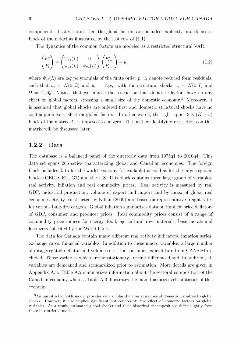
components. Lastly, notice that the global factors are included explicitly into domestic
block of the model as illustrated by the last row of (1.1).
The dynamics of the common factors are modeled as a restricted structural VAR:(F ∗t
Ft
)=
(Ψ11(L) 0
Ψ21(L) Ψ22(L)
)(F ∗t−1
Ft−1
)+ ut (1.2)
where Ψij(L) are lag polynomials of the finite order p, ut denote reduced form residuals,
such that ut ∼ N(0,Ω) and ut = A0et, with the structural shocks et ∼ N(0, I) and
Ω = A0A′0. Notice, that we impose the restriction that domestic factors have no any
effect on global factors, stressing a small size of the domestic economy.3 Moreover, it
is assumed that global shocks are ordered first and domestic structural shocks have no
contemporaneous effect on global factors. In other words, the right upper 3 × (K − 3)
block of the matrix A0 is imposed to be zero. The further identifying restrictions on this
matrix will be discussed later.
1.2.2 Data
The database is a balanced panel of the quarterly data from 1975q1 to 2010q4. This
data set spans 266 series characterizing global and Canadian economies. The foreign
block includes data for the world economy (if available) as well as for the large regional
blocks (OECD, EU, G7) and the U.S. This block contains three large group of variables:
real activity, inflation and real commodity prices. Real activity is measured by real
GDP, industrial production, volume of export and import and by index of global real
economic activity constructed by Kilian (2009) and based on representative freight rates
for various bulk-dry cargoes. Global inflation summarizes data on implicit price deflators
of GDP, consumer and producer prices. Real commodity prices consist of a range of
commodity price indices for energy, food, agricultural raw materials, base metals and
fertilizers collected by the World bank.
The data for Canada contain many different real activity indicators, inflation series,
exchange rates, financial variables. In addition to these macro variables, a large number
of disaggregated deflator and volume series for consumer expenditure from CANSIM in-
cluded. Those variables which are nonstationary are first differenced and, in addition, all
variables are demeaned and standardized prior to estimation. More details are given in
Appendix A.3. Table A.2 summarizes information about the sectoral composition of the
Canadian economy whereas Table A.3 illustrates the main business cycle statistics of this
economy.
3An unrestricted VAR model provides very similar dynamic responses of domestic variables to globalshocks. However, it also implies significant but counterintuitive effect of domestic factors on globalvariables. As a result, estimated global shocks and their historical decompositions differ slightly fromthose in restricted model.

1.2. STRUCTURAL DYNAMIC FACTOR MODEL 7
1.2.3 Estimation
Like in Bernanke et al. (2005), Mumtaz and Surico (2009) and Boivin and Giannoni
(2007), the model was estimated using a two-step principal component analysis (PCA).
In the first step, the PC were extracted from X∗Y,t, X∗π,t, X
∗C,t and Xt to obtain consistent
estimates of the common factors. In the second step, these factors were used for estimation
of the restricted VAR in (1.2).
Note that, in the first step, we impose the constraint that global factors are included
into the principal components for domestic block of the model. So, if these global factors
are really common components, they should be captured by the PC of Xt. To remove the
global factors from the space covered by the PC of Xt, the approach proposed by Boivin
and Giannoni (2007) is used. To do so, the following iterative procedure is adopted
in the first step of the estimation. Starting from the initial estimates of K − 3 principal
components Ft from the domestic block of variablesXt, denoted by F(0)t , iteration proceeds
through the following steps:
1. Regress Xt on F(0)t and estimates of the global factors F ∗Y,t, F
∗π,t and F ∗C,t, to obtain
Λ(0)Y , Λ
(0)π and Λ
(0)C
2. Compute X(0)t = Xt − Λ
(0)Y F ∗Y,t − Λ
(0)π F ∗π,t − Λ
(0)C F ∗C,t
3. Estimate F(1)t as the first K − 3 principal components of X
(0)t
4. Back to the Step 1.
The benchmark model includes 8 factors for Canada. In any case, the impulse re-
sponses do not change significantly if additional domestic factors are considered.4 This
choice implies that the second step in our estimation procedure involves the estimation
of a restricted VAR with 11 endogenous variables: 3 global and 8 domestic factors. Two
lags are included in the model in order to adequately capture its dynamics. This choice
implies a large number of free parameters in the VAR system to be estimated using 144
observations for each variable. Hence, Bayesian methods for estimation of this restricted
VAR are used. Details about the estimation procedure are given in Appendix A.1.
1.2.4 Identification of Structural Shocks
This section discusses the identification of the structural shocks. In particular, we are
interested in identifying three global shocks: i) an unanticipated expansion of global de-
mand (GD), ε∗D,t, ii) a global supply shock, unrelated to commodity markets (GN) , ε∗S,t,
4Bai and Ng (2002) provide several criteria to determine the number of factors present in the dataset, Xt. Their panel information criteria ICp1 and ICp2, for example, suggest the presence respectivelyof 6 and 4 factors in the panel for Canada. However, these criteria do not address directly the questionof how many factors should be included in the VAR.

8 CHAPTER 1. A DYNAMIC FACTOR MODEL FOR CANADA
and iii) a global commodity-specific shock (GC), ε∗C,t. The last shock is aimed to catch
unanticipated changes in the real commodity prices orthogonal to the first two innova-
tions. These changes may be explained by events leading to an unexpected contraction
of the global commodity supply as well as by commodity-specific demand shocks, such as
an increase in the precautionary demand on commodities as a result of expectations of
significant political events.5
Further, since the main goal of this study is to analyze the effect of global shocks on a
small commodity-exporting economy, we are not particularly interested in identifying the
domestic structural shocks. On the contrary, the foreign shocks are identified using two
schemes based on recursive ordering and a mixture of sign and impact matrix restrictions.
In both schemes the foreign factors are ordered first, implying that the rest of the world
does not react instantly to domestic conditions in Canada.
Recursive identification
In the recursive scheme, presented in Table 1.1, the impact matrix corresponding to the
foreign 3× 3 block is lower triangular. The global economic activity factor F ∗Y,t is ordered
first, following by the real commodity price index F ∗C,t and global inflation F ∗π,t respectively.
This ordering implies that the global supply shock has zero contemporaneous effect on
global economic activity and real commodity prices, whereas the commodity-specific shock
does not affect immediately the real activity.
Table 1.1: Recursive identification
Demand Shock, ε∗D,t Commodity Shock, ε∗C,t Supply Shock, ε∗S,tGlobal Economic Activity, u∗Y,t × 0 0
Real Commodity Price, u∗C,t × × 0
Global Inflation, u∗π,t × × ×
This recursive identification is not without limitations. First, it imposes zero restric-
tions on some elements of the impact matrix, in particular, on short-run elasticities of the
global economic activity and real commodity price, respectively, to global supply shock.
However, there is no specific reason for these exclusion restrictions to hold exactly.
Second, as noted by Kilian (2009) and illustrated once again in this paper, impulse
response function of the global economic activity to GC shock is mildly implausible. In
5In contrast to Kilian (2009) we did not identify explicitly commodity supply shocks, given that dataon production and supply of many primary commodities are not so readily available as for the crudeoil market. Moreover, in application to oil market Kilian (2009) and Kilian and Murphy (2010) foundthat relative contribution of the oil supply shock to fluctuations in real oil price is low. A substantialpart of the volatility in the real oil price during 1976-2008 in these papers can be attributed to shocksin global economic activity, with the remainder being largely explained by oil-market specific demandshocks (these speculative demand shocks are ultimately driven by expectations about the availability offuture oil supplies).
1.2. STRUCTURAL DYNAMIC FACTOR MODEL 9
principle, it is quite plausible that this shock implies large response of the real commod-
ity price on impact. Hence, it is reasonable to expect that this spike in the real price
will reduce real activity. Nevertheless, the VAR estimates show that this negative effect
becomes apparent only after one year, whereas small, but significantly positive, response
of the real activity is observed during the first year following the shock.
Thus, to verify the robustness of the results for the recursive scheme, an identification
using sign restrictions on the VAR impulse response function is also used.
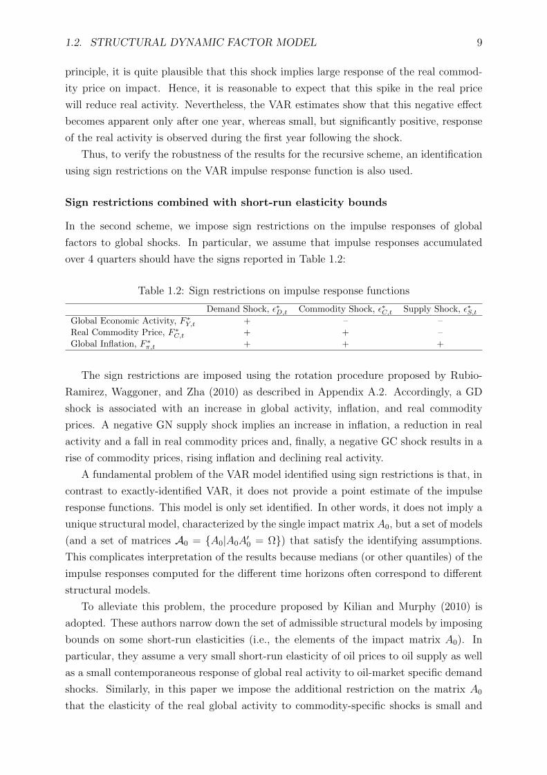
Sign restrictions combined with short-run elasticity bounds
In the second scheme, we impose sign restrictions on the impulse responses of global
factors to global shocks. In particular, we assume that impulse responses accumulated
over 4 quarters should have the signs reported in Table 1.2:
Table 1.2: Sign restrictions on impulse response functions
Demand Shock, ε∗D,t Commodity Shock, ε∗C,t Supply Shock, ε∗S,tGlobal Economic Activity, F ∗Y,t + – –
Real Commodity Price, F ∗C,t + + –
Global Inflation, F ∗π,t + + +
The sign restrictions are imposed using the rotation procedure proposed by Rubio-
Ramirez, Waggoner, and Zha (2010) as described in Appendix A.2. Accordingly, a GD
shock is associated with an increase in global activity, inflation, and real commodity
prices. A negative GN supply shock implies an increase in inflation, a reduction in real
activity and a fall in real commodity prices and, finally, a negative GC shock results in a
rise of commodity prices, rising inflation and declining real activity.
A fundamental problem of the VAR model identified using sign restrictions is that, in
contrast to exactly-identified VAR, it does not provide a point estimate of the impulse
response functions. This model is only set identified. In other words, it does not imply a
unique structural model, characterized by the single impact matrix A0, but a set of models
(and a set of matrices A0 = A0|A0A′0 = Ω) that satisfy the identifying assumptions.
This complicates interpretation of the results because medians (or other quantiles) of the
impulse responses computed for the different time horizons often correspond to different
structural models.
To alleviate this problem, the procedure proposed by Kilian and Murphy (2010) is
adopted. These authors narrow down the set of admissible structural models by imposing
bounds on some short-run elasticities (i.e., the elements of the impact matrix A0). In
particular, they assume a very small short-run elasticity of oil prices to oil supply as well
as a small contemporaneous response of global real activity to oil-market specific demand
shocks. Similarly, in this paper we impose the additional restriction on the matrix A0
that the elasticity of the real global activity to commodity-specific shocks is small and

10 CHAPTER 1. A DYNAMIC FACTOR MODEL FOR CANADA
has not to exceed 5% in abolute terms (|A0(1, 2)| ≤ 0, 05). This implies that only those
structural models satifying these sign and bound restrictions will be kept for the further
analysis.
1.3 Results
This section reports the empirical results of the SDFM presented in the previous section.
First, we discuss estimates of the global factors, namely global economic activity, global
inflation and real commodity price index, illustrate their dynamic response to global
shocks and present historical decompositions of these international factors based on two
alternative identification schemes. Second, using data for Canada, we illustrate the main
stylized facts regarding the effects of international shocks on business cycles in a small
commodity-exporting economy. In particular, we report the dynamic effects of positive
global demand (GD) shock and negative global commodity-specific (GC) shock on terms
of trade and external balances, exchange rates and relative prices, real GDP and its
industrial composition, personal consumption and private investment.
1.3.1 Global common factors and shocks
The global factors were estimated from the international block of the model using pro-
cedure discussed in Section 1.2.1. Figure A.1 plots the estimated principal components
for real activity, inflation and real commodity prices. These factors match closely an
empirical evidence about international business cycles, reported by Kose, Otrok, and
Whiteman (2003) and Mumtaz and Surico (2009), as well as developments in the world
commodity markets, summarized by Hamilton (2011) and Kilian (2006) (in application
to oil markets).
In particular, the global economic activity factor manifests apparently the main global
downturns between 1975q1 and 2010q4: double-dip recession at the beginning of 1980s,
falls in 1991-1993, the East Asian crisis in 1997-1998, slowdown of the early 2000s after
Dot-com bubble collapse and 9/11 attacks, and the Great Recession of the late 2000s.
The real commodity price factor in turn reflects the most important events in commodity
markets: turbulence of the 1978-1981 ignited by the Iranian revolution and outbreak of the
Iran-Iraq war, the oil glut of 1980s, falling commodity prices during the East Asian crisis
in 1997-1998, rising commodity demand in 2000s and downturn in commodity markets
in 2008-2009. The measure of global inflation encompasses stagflation of the 1970s-early
1980s, rising food and energy prices in 2000s as well as deflation of the late 2000s.
Figure A.2 plots the impulse responses of the international factors to global shocks
based on recursive identification (blue line together with 90% credible interval) and the
model with sign restrictions (shaded area covering 90% credible set). Two identification

1.3. RESULTS 11
schemes provide in general similar results. Positive global demand shock generates a
significant expansion in global economic activity, increases global inflation and pushes up
real commodity prices, with maximum effect reached within one year.
An unexpected disruption of global supply (or rising inflation expectations) causes a
decline in real activity, accelerates inflation and depresses real commodity prices. At the
same time, on impact our two identification schemes yield slightly different results for
this shock. Under recursive identification negative supply shock has no immediate effect
on global activity and real commodity prices. It is a consequence of the zero restrictions
imposed in this scheme. In contrast, the model with sign restrictions admits an immediate
negative impact (though not significant at 10% level) of the negative supply shock on real
activity and commodity prices.
Finally, negative commodity-specific shock causes temporary spike in global inflation
and very strong increase in real commodity prices. However, an adverse effect of this shock
on real activity is delayed for one year, and for the model with recursive identification
this negative effect is not very significant.6 Moreover, for the recursive scheme this shock
has small but significant positive effect on global economic activity during the first two-
three quarters. This controversial result is in the line with the findings in Kilian (2009).
The model with sign restrictions avoids this implausible behavior by imposing a negative
accumulated response of the real activity to commodity-specific shock after four quarters.
Figure A.3 plots historical decompositions of the global economic activity, global infla-
tion and real commodity prices based on two alternative structural models. It illustrates
contribution of each of the three global shocks to the dynamics of the international fac-
tors during the period from 1975q1 to 2010q4. The results are virtually invariant to the
method of identification. First, both models suggest that most of the volatility in global
real activity during this period was attributed to global demand shocks. However, positive
supply shocks play an increasing role in driving global economic activity starting from
the middle of 1990s, what may be explained by rising productivity in emerging economies
and trade liberalization. Commodity-specific shocks contributed to economic slowdown
in the beginning of 1980s as well as to revival of global economy after the Asian financial
crisis in 1997-1998.
Second, this figure shows that all three global shocks played an important role in
driving the global inflation. However, in the model with recursive identification an episode
of high inflation in the late 70s-early 80s is attributed in a large extent to the negative
supply shock, whereas the model with sign restrictions explains it mostly by positive
global demand and negative commodity-specific shocks.
And, finally, most of the volatility in the real commodity prices during this period is
6This delayed response of the real output to commodity shock conforms well to the results of Rotem-berg and Woodford (1996) for United States, which show that one percent increase in oil prices leads toa reduction in output of about 0.25 percent after five-seven quarters (with statistically significant declineonly from quarter 3 onwards).

12 CHAPTER 1. A DYNAMIC FACTOR MODEL FOR CANADA
attributed to commodity-specific shocks. This shock catches disruption of oil supply in
the late 70s-early 80s, oil glut of the mid of 80s, region-specific downturn in 1997-1998 and
speculative spike of commodity prices in the beginning of 2008.7 However, a substantial
part of commodity price dynamics is explained by global demand and supply shocks.
In particular, according to this model the Great Recession of the late 2000s was a main
reason of falling commodity prices in 2008-2009. On the other hand, positive global supply
shocks associated with a strong growth in China and India contributed significantly to
the surge in commodity prices in 2000s.
1.3.2 Transmission of international shocks to a small commodity-
exporting economy
This section will illustrate, using data for Canada, a dynamic effect of estimated global
shocks on business cycles in a small commodity-exporting economy. The most interesting
dynamics for this kind of economies is generated by changes in the world commodity prices.
Therefore, we concentrate here on two global shocks explaining most of their volatility,
namely a negative commodity-specific shock and a positive demand shock. These two
shocks induce an increase in commodity prices and, as a result, improve Canada’s terms of
trade, stimulate its external balances and appreciate its real exchange rate. However, their
overall effects on Canadian economy are different, what obscures important regularities
specific to commodity-exporting economies, such as Dutch disease or spending effect.
Terms of trade and external balances effects
We will start a discussion of the results by illustrating terms of trade and external balances
effects.
First, given that Canada is a net exporter of primary commodities, the rising com-
modity prices tend to improve its terms of trade, i.e. a ratio of export and import prices.
It is in contrast with commodity-importing economies, such as United States or Germany,
where commodity prices and terms of trade are negatively correlated. Second, when com-
modity prices are high the current account and trade balances in commodity-exporting
economies tend to rise, whereas at the time of low commodity prices their external bal-
ances plummet. In particular, Kilian et al. (2009) illustrate this positive external balances
effect in application to oil-exporting economies.
7The East Asian financial crisis of 1997-1998 did not generate strong global recession, so our measureof global economic activity fails to account its effect on commodity markets. Moreover, the impact of thiscrisis was different across commodity groups. Oil prices recovered very quickly, and by the end of 1999they were on the pre-crisis level. In contrast, prices of food, wood, base metals and fertilizers stagnateduntil the end of 2003. As a result, our measure of commodity-specific shocks differ slightly from themeasure of oil-market specific demand shocks computed by Kilian (2009), especially for the period after1998.

1.3. RESULTS 13
Figure A.4 plots the impulse responses of the terms of trade and external balances (as
% of GDP) to two global shocks: negative commodity-specific shock and positive global
demand shock. Both shocks significantly increase real commodity prices and improve
terms of trade in Canada. Their effects on external balances are slightly different. An
unanticipated negative commodity-specific shock significantly increases trade and current
account balances. Moreover, this positive effect is almost fully due to increase in trade
balance in primary commodities. In contrast, there is no any evident effect on trade
balance in goods excepting primary commodities. Besides, this shock has strong but
delayed negative effect on real export and no significant and unambiguous effect on real
import, illustrating one of the manifestations of Dutch disease.
Similarly, positive global demand shock increases trade balance in primary commodi-
ties with one-year delay and has no any effect on trade balance in non-commodity goods.
But its effect on total trade and current account balances (as % of GDP) is not so strong
as in the case of negative commodity-specific shock.8 Besides, this positive shock stimu-
lates global economic activity and international trade, so both real export and real import
in Canada significantly increase.
Commodity currency effect and relative prices
Another empirical regularity frequently observed in commodity-exporting economies is
a commodity currency effect. More specifically, real exchange rates in these economies
are usually very volatile and strongly correlated with prices of the exported commodities.
In particular, rising commodity prices result in appreciation of the real exchange rate,
whereas their decrease is associated with the real exchange rate depreciation. This effect
is well studied in the literature. Cashin et al. (2004), for example, analyzed a long-run
cointegrating relationship between the real exchange rates and real prices of exported
commodities for the sample of 58 commodity-exporting countries and found that for 19
of these countries this relationship is statistically significant. Similarly, Chen and Rogoff
(2003) revealed a long-run co-movement of the real exchange rates and real commodity
prices for three developed resource rich economies: Australia, Canada and New Zealand.
Figure A.5 illustrates a commodity currency effect for Canada. Both negative commodity-
specific shock and positive global demand shock result in appreciation of the Canada’s
real effective exchange rate as well as its bilateral real exchange rate with respect to
United States.9 Moreover, this real appreciation in Canada is almost due to appreciation
8Positive global demand shock not only improves Canada’s terms of trade but also significantly in-creases its real GDP. As a result both the nominator (external balances in real terms) and denominator(real GDP) rise, and overall effect of this shock on our measure of external balances (in terms of GDP)is not clear.
9The real exchange rate is defined here as a price of foreign consumption in terms of consumption inCanada, i.e. RERi,CAN,t =
NERi,CAN,tPi,tPCAN,t
, where NERi,CAN,t is a nominal exchange rate in terms of
Canadian dollar per unit of country i currency, Pi,t and PCAN,t are, respectively, foreign and Canadianconsumer price indices. So, an appreciation of the real (nominal) exchange rate in Canada means a

14 CHAPTER 1. A DYNAMIC FACTOR MODEL FOR CANADA
of the nominal exchange rate. At the same time, the ratio of U.S. and Canadian consumer
price indices,PUSA,tPCAN,t
, barely changes after global commodity-specific shocks and slightly
increases in response to global demand shock, reflecting a foreign inflation induced by
rising global demand.
Following Betts and Kehoe (2006, 2008), we decompose the bilateral real exchange
rate RERUS,CAN,t into two components:
RERUS,CAN,t =
(NERUS,CAN,tP
TUS,t
P TCAN,t
)(P TCAN,t
PCAN,t/P TUS,t
PUS,t
)(1.3)
The first component denotes the real exchange rate of traded goods, RERTUS,CAN,t. It
measures deviations from the law of one price for traded goods in Canada and United
States.10 To approximate prices of traded goods we used producer price index in manu-
facturing for these two countries. The second factor, denoted as RERNUS,CAN,t, captures
cross-country differences in internal relative prices. So, if the prices of traded goods satisfy
the law of one price exactly, NERUS,CAN,tPTUS,t = P T
CAN,t, and a composition of consumer
basket is the same across countries, all the dynamics of the real exchange rate will be
attributed to relative changes in prices of non-traded goods,NERUS,CAN,tP
NUS,t
PNCAN,t.
Figure A.5 plots the dynamic effect of global shocks to these two factors. Both shocks
significantly appreciate real exchange rate for traded goods, RERTUS,CAN,t, invalidating
the law of one price. It may be explained by the deficiency of my measure of price index
for traded goods (some goods covered by the PPI are actually non-traded), by cross-
country differences in composition of the baskets for this index, as well as by the fact that
manufacturing prices in two countries are sticky and set in different currencies (at least
for domestic markets).11 This last fact implies that the nominal exchange rate changes
have a strong short-run effect on the real exchange rate for traded goods.
This plot illustrates also a significant but not so strong appreciating effect of the global
commodity-specific shock on the second (relative price) component of the real exchange
rate in Canada, RERNUS,CAN,t. That is in line with the results in Betts and Kehoe (2006)
which observed positive correlation between bilateral U.S./Canada real exchange rate and
its relative price factor. In contrast, global demand shock yields only very week internal
appreciation on impact, whereas after one year this measure of the real exchange rate
tends to depreciate following rising global inflation.
Figure A.5 reports also the effect of global shocks on disaggregated prices, namely on
the implicit price deflators for disaggregated groups of personal consumption in Canada
(as in Boivin, Giannoni, and Mihov, 2009). There is strong evidence of heterogeneity
decrease in RERi,CAN,t (NERi,CAN,t).10Notice that this ratio is also affected by any differences in the compositions of the baskets of traded
goods across countries.11Notice, however, that 96% of Canadian export to United States are priced in U.S. dollars (Gopinath
and Rigobon, 2008).

1.3. RESULTS 15
in responses. Both shocks generate strong immediate positive effect on energy prices,
whereas the rest of prices manifest diverse dynamics. In the long run, however, there is
rising trend in prices of non-energy goods, reflecting increased costs of their production
in an environment of high commodity prices.
Spending effect and Backus-Smith puzzle
Soaring commodity prices significantly improve terms of trade in Canada and generate
windfall revenues from its commodity export, as shown in Section 1.3.2. Their overall
effect on economy depends crucially on the way this windfall income is spent. A positive
response of external balances in Canada to negative commodity-specific shock (and to a
lesser extent to positive global demand shock) signals that at least a part of commodity
revenues is saved abroad, leveling their effect on domestic economy. However, the rest of
this income is spent inside the country affecting its output and final expenditures.
Figure A.6 illustrates this spending effect for Canadian economy. Negative commodity-
specific shock has no any significant effect on real GDP in Canada. Total employment
and total industrial capacity utilization are barely affected too. That is in contrast to
its strong12 but delayed negative effect on global economic activity. Moreover, this shock
has positive and significant impact on final domestic expenditures in Canada. Most of
this growth is explained by increasing current expenditures of government, enjoying a
surge in tax revenues from commodity sector, and real private investments. Real personal
consumption expenditures also manifest a small positive response on impact, but this
effect disappears very quickly.
In contrast to negative commodity-specific shock, positive global demand shock stim-
ulates global economic activity and international trade. As a result, this shock has signifi-
cant and unambiguous positive effect on real GDP and real final domestic expenditures in
Canada, as well as on its total employment and industrial capacity utilization. This strong
growth is triggered mostly by higher foreign demand and obscures an immediate effect of
windfall income from commodity export. Besides, real current government expenditures
do not change whereas real government investment gradually decreases, signaling about
countercyclical character of fiscal policy.
Now we will look more closely at the effects of global shocks on personal consumption
in Canada. Figure A.7 illustrates impulse responses of the real expenditures on large
aggregated groups of goods, namely on durable and semi-durable goods, and services, as
well as on disaggregated series. Implications of the negative commodity-specific shock
for aggregated groups are very similar to that for total real consumption. However,
dynamic responses of disaggregated goods (except of energy and food) are mostly positive,
whereas disaggregated services illustrate no uniform dynamics, indicating that there is a
12at least for the model with sign restrictions

16 CHAPTER 1. A DYNAMIC FACTOR MODEL FOR CANADA
small (but insignificant) substitution effect.13 In contrast, a positive global demand shock
has an uniform and strong positive effect on all aggregated and disaggregated groups of
consumption.14
Another interesting fact is associated with relative consumption, i.e. ratio of real
personal consumption expenditures, between Canada and United States. An empiri-
cal evidence suggests that relative consumption across countries, does not move in any
systematic way with its relative price, i.e. real exchange rate. That is in contrast to pre-
dictions of many international business cycle models assuming perfect financial markets,
which suggest that consumption should be higher in the country where its price, con-
verted into a common currency is lower. This collision is known in an economic literature
as consumption-real exchange rate anomaly or Backus-Smith puzzle (Backus and Smith,
1993). Although this puzzle is observed not only for commodity-exporting economies, for
the last group it is especially pronounced. Negative, not predicted positive, correlation
of the relative consumption and real exchange rate is often reported for these countries.
Along with volatile and negatively correlated with commodity price real exchange rate it
may be considered as a signal of imperfections in international risk sharing.
Figure A.7 plots dynamic responses of the relative consumption between Canada and
United States to global shocks. As shown earlier, negative commodity-specific shock has
only a small and short-living positive effect on real personal consumption in Canada.
However, it implies a strong and permanent positive response of relative consumption
between Canada and United States. Given that real exchange rate appreciates after this
shock, this shock generates strong negative correlation between relative consumption and
its relative price, illustrating Backus-Smith puzzle and indicating about imperfections
in risk sharing between these two countries. In contrast, positive global demand shock
results in a strong growth of personal consumption in Canada but has no any significant
effect on its relative consumption with United States. This last fact, however, does not
say that global demand shocks are perfectly insured. A full risk sharing would imply
instead a decrease in personal consumption relative to United States, following its rising
relative price (appreciating real exchange rate).
13Recall, that negative commodity-specific shock results in an appreciation of the relative price com-ponent of the real exchange rate. Besides, there is some evidence (not reported in this paper) that afterthis shock the prices of durable consumer goods decrease relative to prices of services.
14Figure A.7 reports two counterintuitive negative responses of disaggregated series for services afterpositive global demand shock. However, it is simply an incidental result of demeaning and normalizationprocedure, essential for an extraction of principal components. These two series correspond to ’grossimputed rent’ and ’gross paid rent’ (in constant prices), which barely manifest any volatility exceptof long-run rising trend. Without normalization (by standard deviations) these responses were hardlydistinguishable from zero.

1.3. RESULTS 17
Investment effect
Section 1.3.2 illustrates that a substantial portion of the windfall revenues from com-
modity export in Canada is channeled into the real private investments in fixed capital.
However, in addition to this direct spending effect, there is another indirect propagation
mechanism of global shocks to private investment growth. More specifically, an apprecia-
tion of the real exchange rate, associated with an increase in commodity prices, results in
decreasing relative prices of investment goods, which are predominantly tradable. As a
result, investment demand increases. Much of this investment goes into the nontradable
and commodity-producing sectors of the economy (see Spatafora and Warner, 1999).
Figure A.8 plots impulse responses of the business gross fixed capital formation, as well
as its components and prices, to global shocks. As shown earlier, negative commodity-
specific shock generates a positive response of the total real investment in Canada. Be-
sides, its price deflator initially decreases following appreciation of the nominal exchange
rate. That is in contrast to consumer price index, which increases after a spike in com-
modity prices. Moreover, most of this deflation is explained by its tradable component,
namely ’machinery and equipment’, whereas price deflators of the investments in resi-
dential and non-residential structures (produced by non-tradable construction) tend to
increase. However, a main growth engine of the private investment after this global shock
is an investment in non-residential structures. Investment in machinery and equipment
increases too, but its growth is not so strong. Besides, residential investments are barely
affected by this shock.
Positive global demand shock has similar implications for the price deflators of private
investment in fixed capital. Price index of total investment slightly decreases on impact
with most of this decrease explained by investment in machinery and equipment. However,
in contrast to negative commodity-specific shock, this positive shock results in a strong
growth of all investment components, including residential investments.
Dutch disease
Dutch disease is perhaps the most famous phenomenon associated with commodity-
exporting economies. This economic concept explains a relationship between an increase
in export revenues from primary commodities and a decline in the non-commodity trad-
able sector, mainly manufacturing. The underlying mechanism is the following. An
increase in export of primary commodities will appreciate real exchange rate, making
non-commodity exports more expensive. As a result, the manufacturing sector becomes
less competitive and its output declines, whereas output of nontradable and commodity
sectors increases. Simultaneously, labor and capital move from manufacturing to booming
sectors of the economy (see Corden, 1984, for more details).
Dutch disease effect is well-studied in economic literature (see Stijns, 2003, for good re-

18 CHAPTER 1. A DYNAMIC FACTOR MODEL FOR CANADA
view). However, there is striking absence of unambiguous evidence for this phenomenon
from data. For example, Spatafora and Warner (1999) fails to detect a contraction in
manufacturing sector after oil price shock for a group of developing oil-exporting coun-
tries. In contrast, using gravity trade model and international trade data, Stijns (2003)
reports that a one percent increase in world energy price is estimated to decrease real
manufacturing exports from energy-exporting economy by almost half a percent. The
main reason of these disagreements is that it is very difficult to disentangle relative price
effects of commodity price fluctuations from their impact on the domestic and interna-
tional macroeconomic conditions. Besides, these commodity price changes themselves
may be results of changing global demand or supply.
An empirical model presented in this paper illustrates these difficulties. Figure A.9
plots impulse responses of the real GDP in the main sectors of Canadian economy, namely
in mining, manufacturing, services, utilities and construction, as well as for disaggre-
gated industries in manufacturing and services, to negative commodity-specific shock and
positive global demand shock. Strikingly, these two shocks imply completely different
structural dynamics in a small commodity-exporting economy.
As in Section 1.3.2, negative commodity-specific shock has no any evident effect on
the aggregate output. However, real GDP responses for the main sectors are very di-
verse, illustrating Dutch disease symptoms. First, this shock has significant positive
effect on commodity-producing tradable sector, mining, with a maximum increase after
3 quarters. Nontradable sectors reap the benefits too. Real GDP in services has statisti-
cally significant increase on impact, construction and utilities are booming. In contrast,
non-commodity tradable sector, manufacturing, unambiguously declines following van-
ishing foreign demand, with a maximum decrease in output after one year.15 Second,
impulse responses of disaggregated series for manufacturing and services illustrate the
same pattern. Manufacturing industries tend to decrease with the lapse of time, whereas
service-producing industries are slightly rising initially but their dynamics become dis-
perse afterwards.
Positive global demand shock also increases the real commodity prices and appreciates
the real exchange rate. But, in contrast to negative commodity-specific shock, its effect
on real GDP in industries is uniform: positive increase in output with the maximum effect
after 3-4 quarters. Taking into account that these two shocks explains a sizable part of
the volatility in commodity prices and domestic and global economic activity, it is not
surprise that Dutch disease is so often undetectable in data.
Figure A.10 supplements this story with dynamic responses of capacity utilization
and employment. Negative commodity-specific shock has no any significant effect on to-
tal industrial capacity utilization. However, this shock implies more intensive capacity
utilization in mining, more excess capacity in manufacturing and no any significant re-
15Recall from Section 1.3.2 that real export is declining too.

1.4. CONCLUSIONS 19
sponse in construction. In contrast, number of employed in industries hardly changes,
except of construction, where employment slightly increases after 2-3 quarters. Positive
global demand shock in turn has strong and uniform positive effect on capacity utilization
and employment across industries.
Monetary policy and financial variables
To finish the discussion, we report here dynamic responses of the selected monetary and
financial indicators in Canada. Both negative commodity-specific shock and positive
global demand shock imply strong growth in the S&P/TSX Composite Index. It is not
very surprising taking into account that more mining and oil&gas companies are listed
on Toronto Stock Exchange than on any other exchange in the world.
Another interesting question is how monetary authority in Canada responds to global
shocks. Several observations are worth mentioning. First, total foreign exchange reserves
are hardly changes after these two shocks indicating that Canadian dollar floats freely
and the Bank of Canada does not intervene systematically in foreign exchange markets in
response to changing international macroeconomic conditions. Second, there is a weak in-
dication that Bank of Canada responds to negative commodity-specific shock by lowering
interest rates. However, the model with sign restrictions says that this effect is insignif-
icant. In contrast, Bank of Canada unambiguously rises its interest rates in response to
positive global demand shocks, fighting excessive foreign demand and inflation.
And, finally, both shocks result in an endogenous expansion of banking credit and
broad money, though for the negative commodity-specific shock this effect is not very
strong.
1.4 Conclusions
This paper studied the effect of international shocks on a small commodity-exporting econ-
omy. Using structural factor model we quantified the dynamic effects of a wide variety of
Canadian variables to two global shocks, explaining the most of the volatility in real com-
modity prices, namely to negative commodity-specific shock and to positive innovation in
global demand. Then we illustrated the main stylized facts regarding the effects of fluc-
tuations in the real commodity prices on business cycles in a small commodity-exporting
economy.
This paper supports the viewpoint that commodity prices are driven by several global
shocks. In particular, global demand shock, commodity-specific shock and global non-
commodity supply shock contributed significantly to changes in the real commodity prices
during observed period, with the first two shocks explaining most of their volatility. More-
over, both positive global demand shock and negative commodity-specific shocks result

20 CHAPTER 1. A DYNAMIC FACTOR MODEL FOR CANADA
in increasing commodity prices and generate positive effect on external balances, com-
modity currency effect, Backus-Smith anomaly and positive investment effect in Canada.
However, Dutch disease and spending effect are clearly illustrated only by the negative
commodity-specific shock. In contrast, positive innovation in global demand stimulates
real output and real expenditures uniformly across industries and sectors of the Cana-
dian economy without any indication of the Dutch disease or spending effect. Given that
global demand shock contributes significantly to commodity price volatility, this fact can
explain why Dutch disease effect is so strikingly absent in the data.

Appendix A
Appendices to Chapter 1
A.1 Estimation method
The restricted VAR has a different set of explanatory variables in each equation and may be estimated
as a system of seemingly unrelated regressions (SUR). In particular, we can write this system as
yt = Xtβ + εt (A.1)
where yt =(y1t y2t . . . yKt
)′, β =
(β′1 β′2 . . . β′K
)′, Xt is a block-diagonal matrix with blocks
x′kt containing the t-th observation of the vector of explanatory variables relevant for the k-th variable
and εt =(ε1t ε2t . . . εKt
)′with εt ∼ N(0,Σ).
A Bayesian estimator of the restricted VAR was employed in this paper (see Koop, Poirier, and
Tobias, 2007). A commonly used prior for this model is an independent normal-Wishart prior:
p(β,Σ−1) ∝ φ(β|β, V )fW (Σ−1|H, v)
with φ(·) and fW (·) denoting respectively Normal and Wishart probability density functions.
The conditional posterior distribution of the VAR coefficients is given then by:
β|y,Σ−1 ∼ N(β, V ) (A.2)
where V =(V −1 +
∑Tt=1X
′tΣ−1Xt
)−1and β = V
(V −1β +
∑Tt=1X
′tΣ−1yt
).
The posterior for Σ−1 conditional on β is computed as:
Σ−1|y, β ∼W (H, v) (A.3)
where H =(H−1 +
∑Tt=1(yt −Xtβ)(yt −Xtβ)′
)−1and v = T + v.
In this paper we assume an uninformative prior: V −1 = 0, v = 0 and H−1 = 0. To approximate
the posterior distribution in the model we use a Gibbs sampler that sequentially draws from the normal
φ(β|y,Σ−1) and the Wishart fW (Σ−1|y, β).
21

22 APPENDIX A. APPENDICES TO CHAPTER 1
A.2 Identification using sign and bound restrictions
The sign restrictions are imposed using procedure based on Rubio-Ramirez et al. (2010). Let B0 be
a structural impact matrix computed using the Cholesky decomposition of the reduced form variance-
covariance matrix Ω with the global factors ordered first, i.e. Ω = B0B′0. Let Q be identity matrix with
the foreign (upper-left) block substituted by any (rotational) orthogonal 3×3 matrix, such that QQ′ = I.
Then, multiplying the impact matrix B0 by Q yields a new structural impact matrix B0 = B0Q (with
the global factors ordered first again). Notice, that B0B′0 = Ω. Drawing repeatedly from the set of
orthogonal rotational matrices one can generate a wide range of possible choices for the structural model.
The algorithm consists of the following steps:
1. Compute the Cholesky decomposition Bk0 of the posterior draw k of the reduced form variance-
covariance matrix Ωk with the global factors ordered first.
2. Draw an independent standard normal 3× 3 matrix X and let X = QR be the QR decomposition
of X with the diagonal of R normalized to be positive. Then Q is a rotational orthogonal matrix
and has the uniform (or Haar) distribution. Substitute the upper-left diagonal block of the identity
matrix Q by Q.
3. Compute Ak0 = Bk0 Q. If this model satisfies the sign and bound restrictions, keep it. Otherwise,
move to the next Gibbs iteration.

A.3. DESCRIPTION OF DATA 23
A.3 Description of data
Data span the period from the first quarter of 1975 to the forth quarter of 2010. The format contains:
i) series code, ii) description, iii) source of data, iv) transformation code and v) variance explained by
its common components. The transformation codes are: 1 – no transformation; 2 – first difference;
4 – logarithm; 5 – first difference of logarithm. The data set contains 266 quarterly series with no
missing observations. The main sources of data are OECD EO, World bank GEM, CANSIM and FRED2
databases.
Global Economic Activity Series
Series ID Title Source Code R2
1 GDP-OECD Real gross domestic product, OECD, SA OECD 5 0,88
2 GDP-G7 Real gross domestic product, G7, SA OECD 5 0,80
3 GDP-EU15 Real gross domestic product, EU15, SA OECD 5 0,67
4 GDP-US Real gross domestic product, USA, SA OECD 5 0,50
5 IND-G7 Industrial production index, G7, SA OECD 5 0,91
6 IND-EU Industrial production index, OECD Europa, SA OECD 5 0,78
7 IND-US Industrial production index, USA, SA OECD 5 0,69
8 EXP-WORLD Export (volume), World, SA OECD 5 0,81
9 EXP-OECD Export (volume), OECD, SA OECD 5 0,84
10 IMP-WORLD Import (volume), World, SA OECD 5 0,82
11 IMP-OECD Import (volume), OECD, SA OECD 5 0,85
12 DCBFR Index of Dry Cargo Bulk Freight Rates Kilian (2009) 2 0,09
Global Inflation Series
Series ID Title Source Code R2
1 DGDP-OECD Deflator of gross domestic product, OECD, SA OECD 5 0,88
2 DGDP-G7 Deflator of gross domestic product, G7, SA OECD 5 0,88
3 DGDP-EU Deflator of gross domestic product, OECD Europa, SA OECD 5 0,83
4 DGDP-EU15 Deflator of gross domestic product, EU15, SA OECD 5 0,84
5 DGDP-US Deflator of gross domestic product, USA, SA OECD 5 0,88
6 CPI-OECD Consumer price index, all items, OECD, SA OECD 5 0,82
7 CPI-G7 Consumer price index, all items, G7, SA OECD 5 0,92
8 CPI-EU Consumer price index, all items, OECD Europa, SA OECD 5 0,70
9 CPI-US Consumer price index, all items, USA, SA OECD 5 0,80
10 CPINEF-OECD Consumer price index, all items, non-food, non-energy, OECD, SA OECD 5 0,68
11 CPINEF-G7 Consumer price index, all items, non-food, non-energy, G7, SA OECD 5 0,85
12 CPINEF-EU Consumer price index, all items, non-food, non-energy, OECD Europa, SA OECD 5 0,64
13 CPINEF-US Consumer price index, all items, non-food, non-energy, USA, SA OECD 5 0,82
14 PPIM-US Total producer prices, manufacturing, USA, SA OECD 5 0,43
15 PPIFG-US Total producer prices, finished goods, USA, SA OECD 5 0,49
Real Commodity Prices Series
Series ID Title Source Code R2
1 RCP-ENERGY Commodity price index, constant 2000 US$, Energy, SA WB - GEM 5 0,54
2 RCP-FOOD Commodity price index, constant 2000 US$, Agr., Food, SA WB - GEM 5 0,48
3 RCP-RAW Commodity price index, constant 2000 US$, Agr., Raw Materials, SA WB - GEM 5 0,59
4 RCP-METALS Commodity price index, constant 2000 US$, Base Metals, SA WB - GEM 5 0,61
5 RCP-FERT Commodity price index, constant 2000 US$, Fertilizers, SA WB - GEM 5 0,25
Canadian Economy Series
Gross domestic product, expenditure-based, constant 2002 prices
Series ID Title Source Code R2
1 GDP-CAN Gross domestic product at market prices, SA CANSIM 5 0,75
2 PC-CAN Personal expenditure on consumer goods and services, SA CANSIM 5 0,88
3 PCG-CAN Personal expenditure on consumer goods, SA CANSIM 5 0,75
4 PCDUR-CAN Personal expenditure on durable goods, SA CANSIM 5 0,63
5 PCSDUR-CAN Personal expenditure on semi-durable goods, SA CANSIM 5 0,78
6 PCNDUR-CAN Personal expenditure on non-durable goods, SA CANSIM 5 0,42
7 PCSER-CAN Personal expenditure on services, SA CANSIM 5 0,54
8 GC-CAN Government current expenditure on goods and services, SA CANSIM 5 0,09
9 GGFC-CAN Government gross fixed capital formation, SA CANSIM 5 0,23
10 GINV-CAN Government investment in inventories, SA CANSIM 1 0,29
11 BGFC-CAN Business gross fixed capital formation, SA CANSIM 5 0,76
12 RES-CAN Residential structures, SA CANSIM 5 0,56
13 NRESEQ-CAN Non-residential structures and equipment, SA CANSIM 5 0,69
14 NRES-CAN Non-residential structures, SA CANSIM 5 0,51
15 EQ-CAN Machinery and equipment, SA CANSIM 5 0,57
16 BINV-CAN Business investment in inventories, SA CANSIM 1 0,60
17 BNFINV-CAN Business investment in non-farm inventories, SA CANSIM 1 0,60
18 BFINV-CAN Business investment in farm inventories, SA CANSIM 1 0,06
19 EXP-CAN Exports of goods and services, SA CANSIM 5 0,69

24 APPENDIX A. APPENDICES TO CHAPTER 1
20 EXPG-CAN Exports of goods, SA CANSIM 5 0,66
21 EXPS-CAN Exports of services, SA CANSIM 5 0,24
22 IMP-CAN Imports of goods and services, SA CANSIM 5 0,69
23 IMPG-CAN Imports of goods, SA CANSIM 5 0,65
24 IMPS-CAN Imports of services, SA CANSIM 5 0,45
25 FDD-CAN Final domestic demand, SA CANSIM 5 0,85
Gross domestic product, expenditure-based, implicit price deflator
Series ID Title Source Code R2
26 PGDP-CAN Gross domestic product, SA CANSIM 5 0,81
27 PPC-CAN Personal expenditure on consumer goods and services, SA CANSIM 5 0,93
28 PPCG-CAN Personal expenditure on consumer goods, SA CANSIM 5 0,86
29 PPCDUR-CAN Personal expenditure on durable goods, SA CANSIM 5 0,65
30 PPCSDUR-CAN Personal expenditure on semi-durable goods, SA CANSIM 5 0,79
31 PPCNDUR-CAN Personal expenditure on non-durable goods, SA CANSIM 5 0,77
32 PPCSER-CAN Personal expenditure on services, SA CANSIM 5 0,86
33 PGC-CAN Government current expenditure on goods and services, SA CANSIM 5 0,56
34 PGGFC-CAN Government gross fixed capital formation, SA CANSIM 5 0,61
35 PBGFC-CAN Business gross fixed capital formation, SA CANSIM 5 0,64
36 PRES-CAN Residential structures, SA CANSIM 5 0,37
37 PNRESEQ-CAN Non-residential structures and equipment, SA CANSIM 5 0,75
38 PNRES-CAN Non-residential structures, SA CANSIM 5 0,54
39 PEQ-CAN Machinery and equipment, SA CANSIM 5 0,77
40 PEXP-CAN Exports of goods and services, SA CANSIM 5 0,69
41 PEXPG-CAN Exports of goods, SA CANSIM 5 0,68
42 PEXPS-CAN Exports of services, SA CANSIM 5 0,70
43 PIMP-CAN Imports of goods and services, SA CANSIM 5 0,89
44 PIMPG-CAN Imports of goods, SA CANSIM 5 0,86
45 PIMPS-CAN Imports of services, SA CANSIM 5 0,86
46 PFDD-CAN Final domestic demand, SA CANSIM 5 0,94
Exchange rates and external balances
Series ID Title Source Code R2
47 NEER-CAN Nominal Effective Exchange Rate BIS 5 0,79
48 NERUS-CAN Bilateral Nominal Exchange Rate, CAD/USD CANSIM 5 0,87
49 REER-CAN Real Effective Exchange Rate BIS 5 0,79
50 RERUS-CAN Bilateral Real Exchange Rate, Canada vs. USA CANSIM 5 0,88
51 RERT-CAN Real Exchange Rate, traded goods (PPI) CANSIM 5 0,78
52 RERN-CAN Real Exchange Rate, internal relative prices (PPI/CPI) CANSIM 5 0,56
53 CA-CAN Current account balance, % of GDP, SA CANSIM 1 0,72
54 TB-CAN Trade balance (goods and services), % of GDP, SA CANSIM 1 0,70
55 TBG-CAN Trade balance (goods, all types), % of GDP, SA CANSIM 1 0,69
56 TBC-CAN Trade balance (goods, primary commodities), % of GDP, SA CANSIM 1 0,66
57 TBNC-CAN Trade balance (goods, except of primary commodities), % of GDP, SA CANSIM 1 0,63
Personal expenditures, constant 2000 prices
Series ID Title Source Code R2
58 PCDIF-CAN-US Personal consumption differential in Canada and USA, logs, SA CANSIM, FRED2 2 0,53
59 PCFNAB-CAN Food and non-alcoholic beverages, SA CANSIM 5 0,19
60 PCAB-CAN Alcoholic beverages bought in stores, SA CANSIM 5 0,21
61 PCTOB-CAN Tobacco products, SA CANSIM 5 0,16
62 PCMBC-CAN Men’s and boys’ clothing, SA CANSIM 5 0,55
63 PCWGC-CAN Women’s, girl’s and children’s clothing, SA CANSIM 5 0,51
64 PCFW-CAN Footwear, SA CANSIM 5 0,44
65 PCGIR-CAN Gross imputed rent, SA CANSIM 5 0,39
66 PCGPR-CAN Gross paid rent, SA CANSIM 5 0,29
67 PCOS-CAN Other shelter expenses, SA CANSIM 5 0,29
68 PCEL-CAN Electricity, SA CANSIM 5 0,17
69 PCNG-CAN Natural gas, SA CANSIM 5 0,36
70 PCOF-CAN Other fuels, SA CANSIM 5 0,31
71 PCFC-CAN Furniture, carpets and other floor coverings, SA CANSIM 5 0,57
72 PCHA-CAN Household appliances, SA CANSIM 5 0,67
73 PCSDF-CAN Semi-durable household furnishings, SA CANSIM 5 0,64
74 PCNHS-CAN Non-durable household supplies, SA CANSIM 5 0,32
75 PCDCC-CAN Domestic and child care services, SA CANSIM 5 0,15
76 PCOHS-CAN Other household services, SA CANSIM 5 0,18
77 PCMC-CAN Medical care, SA CANSIM 5 0,18
78 PCHC-CAN Hospital care and the like, SA CANSIM 5 0,44
79 PCOMC-CAN Other medical care expenses, SA CANSIM 5 0,15
80 PCDPH-CAN Drugs and pharmaceutical products, SA CANSIM 5 0,16
81 PCNUMV-CAN New and used (net) motor vehicles, SA CANSIM 5 0,44
82 PCMVRP-CAN Motor vehicle repairs and parts, SA CANSIM 5 0,19
83 PCMFL-CAN Motor fuels and lubricants, SA CANSIM 5 0,29
84 PCOAR-CAN Other auto related services, SA CANSIM 5 0,21
85 PCPT-CAN Purchased transportation, SA CANSIM 5 0,26
86 PCCOM-CAN Communications, SA CANSIM 5 0,27
87 PCRSC-CAN Recreational, sporting and camping equipment, SA CANSIM 5 0,66

A.3. DESCRIPTION OF DATA 25
88 PCRES-CAN Reading and entertainment supplies, SA CANSIM 5 0,47
89 PCRS-CAN Recreational services, SA CANSIM 5 0,26
90 PCECS-CAN Education and cultural services, SA CANSIM 5 0,05
91 PCPE-CAN Personal effects not elsewhere classified, SA CANSIM 5 0,31
92 PCPC-CAN Personal care, SA CANSIM 5 0,27
93 PCRAS-CAN Restaurants and accommodation services, SA CANSIM 5 0,46
94 PCFLS-CAN Financial and legal services, SA CANSIM 5 0,12
95 PCNPO-CAN Operating expenses of non-profit organizations, SA CANSIM 5 0,11
Personal expenditures, implicit price deflator
Series ID Title Source Code R2
96 PPCFNAB-CAN Food and non-alcoholic beverages, SA CANSIM 5 0,45
97 PPCAB-CAN Alcoholic beverages bought in stores, SA CANSIM 5 0,55
98 PPCTOB-CAN Tobacco products, SA CANSIM 5 0,28
99 PPCMBC-CAN Men’s and boys’ clothing, SA CANSIM 5 0,60
100 PPCWGC-CAN Women’s, girl’s and children’s clothing, SA CANSIM 5 0,55
101 PPCFW-CAN Footwear, SA CANSIM 5 0,58
102 PPCGIR-CAN Gross imputed rent, SA CANSIM 5 0,78
103 PPCGPR-CAN Gross paid rent, SA CANSIM 5 0,81
104 PPCOS-CAN Other shelter expenses, SA CANSIM 5 0,15
105 PPCEL-CAN Electricity, SA CANSIM 5 0,38
106 PPCNG-CAN Natural gas, SA CANSIM 5 0,23
107 PPCOF-CAN Other fuels, SA CANSIM 5 0,56
108 PPCFC-CAN Furniture, carpets and other floor coverings, SA CANSIM 5 0,47
109 PPCHA-CAN Household appliances, SA CANSIM 5 0,65
110 PPCSDF-CAN Semi-durable household furnishings, SA CANSIM 5 0,72
111 PPCNHS-CAN Non-durable household supplies, SA CANSIM 5 0,67
112 PPCDCC-CAN Domestic and child care services, SA CANSIM 5 0,37
113 PPCOHS-CAN Other household services, SA CANSIM 5 0,18
114 PPCMC-CAN Medical care, SA CANSIM 5 0,73
115 PPCHC-CAN Hospital care and the like, SA CANSIM 5 0,42
116 PPCOMC-CAN Other medical care expenses, SA CANSIM 5 0,19
117 PPCDPH-CAN Drugs and pharmaceutical products, SA CANSIM 5 0,71
118 PPCNUMV-CAN New and used (net) motor vehicles, SA CANSIM 5 0,53
119 PPCMVRP-CAN Motor vehicle repairs and parts, SA CANSIM 5 0,68
120 PPCMFL-CAN Motor fuels and lubricants, SA CANSIM 5 0,58
121 PPCOAR-CAN Other auto related services, SA CANSIM 5 0,19
122 PPCPT-CAN Purchased transportation, SA CANSIM 5 0,38
123 PPCCOM-CAN Communications, SA CANSIM 5 0,22
124 PPCRSC-CAN Recreational, sporting and camping equipment, SA CANSIM 5 0,60
125 PPCRES-CAN Reading and entertainment supplies, SA CANSIM 5 0,52
126 PPCRS-CAN Recreational services, SA CANSIM 5 0,45
127 PPCECS-CAN Education and cultural services, SA CANSIM 5 0,49
128 PPCPE-CAN Personal effects not elsewhere classified, SA CANSIM 5 0,33
129 PPCPC-CAN Personal care, SA CANSIM 5 0,72
130 PPCRAS-CAN Restaurants and accommodation services, SA CANSIM 5 0,74
131 PPCFLS-CAN Financial and legal services, SA CANSIM 5 0,19
132 PPCNPO-CAN Operating expenses of non-profit organizations, SA CANSIM 5 0,66
Gross domestic product, by industry, constant 2000 prices
Series ID Title Source Code R2
133 GDPBS-CAN Business sector, goods, SA CANSIM 5 0,90
134 GDPBSS-CAN Business sector, services, SA CANSIM 5 0,70
135 GDPGI-CAN Goods producing industries, SA CANSIM 5 0,90
136 GDPSI-CAN Services producing industries, SA CANSIM 5 0,68
137 GDPIP-CAN Industrial production, SA CANSIM 5 0,92
138 GDPAGR-CAN Agriculture, forestry, fishing and hunting, SA CANSIM 5 0,13
139 GDPMIN-CAN Mining and oil and gas extraction, SA CANSIM 5 0,29
140 GDPUT-CAN Utilities, SA CANSIM 5 0,46
141 GDPCON-CAN Construction, SA CANSIM 5 0,45
142 GDPMAN-CAN Manufacturing, SA CANSIM 5 0,92
143 GDPFOOF-CAN Food manufacturing, SA CANSIM 5 0,19
144 GDPBEV-CAN Beverage and tobacco product manufacturing, SA CANSIM 5 0,27
145 GDPTEX-CAN Textile and textile product mills, SA CANSIM 5 0,54
146 GDPCLO-CAN Clothing manufacturing, SA CANSIM 5 0,34
147 GDPLET-CAN Leather and allied product manufacturing, SA CANSIM 5 0,27
148 GDPWOOD-CAN Wood product manufacturing, SA CANSIM 5 0,48
149 GDPPAP-CAN Paper manufacturing, SA CANSIM 5 0,34
150 GDPPRI-CAN Printing and related support activities, SA CANSIM 5 0,35
151 GDPPET-CAN Petroleum and coal products manufacturing, SA CANSIM 5 0,31
152 GDPCHE-CAN Chemical manufacturing, SA CANSIM 5 0,54
153 GDPPL-CAN Plastics and rubber products manufacturing, SA CANSIM 5 0,69
154 GDPNMM-CAN Non-metallic mineral product manufacturing, SA CANSIM 5 0,62
155 GDPPRM-CAN Primary metal manufacturing, SA CANSIM 5 0,58
156 GDPFM-CAN Fabricated metal product manufacturing, SA CANSIM 5 0,67
157 GDPMACH-CAN Machinery manufacturing, SA CANSIM 5 0,57
158 GDPCEL-CAN Computer and electronic product manufacturing, etc., SA CANSIM 5 0,42
159 GDPTREQ-CAN Transportation equipment manufacturing, SA CANSIM 5 0,51

26 APPENDIX A. APPENDICES TO CHAPTER 1
160 GDPFUN-CAN Furniture and related product manufacturing, SA CANSIM 5 0,57
161 GDPMISC-CAN Miscellaneous manufacturing, SA CANSIM 5 0,23
162 GDPWHT-CAN Wholesale trade, SA CANSIM 5 0,55
163 GDPRET-CAN Retail trade, SA CANSIM 5 0,44
164 GDPTRAN-CAN Transportation and warehousing, SA CANSIM 5 0,51
165 GDPINF-CAN Information and cultural industries, SA CANSIM 5 0,36
166 GDPFIN-CAN Finance, insurance, real estate, etc., SA CANSIM 5 0,16
167 GDPPR-CAN Professional, scientific and technical services, SA CANSIM 5 0,27
168 GDPEDUC-CAN Educational services, SA CANSIM 5 0,15
169 GDPHEA-CAN Health care and social assistance, SA CANSIM 5 0,35
170 GDPACC-CAN Accommodation and food services, SA CANSIM 5 0,46
171 GDPOTHS-CAN Other services (except public administration), SA CANSIM 5 0,39
172 GDPPA-CAN Public administration, SA CANSIM 5 0,14
Capacity Utilization
Series ID Title Source Code R2
173 CUIND-CAN Total industrial, SA CANSIM 5 0,87
174 CUFOR-CAN Forestry and logging, SA CANSIM 5 0,12
175 CUMOG-CAN Mining and oil and gas extraction, SA CANSIM 5 0,33
176 CUEPG-CAN Electric power generation, transmission and distribution, SA CANSIM 5 0,37
177 CUCON-CAN Construction, SA CANSIM 5 0,41
178 CUMAN-CAN Manufacturing, SA CANSIM 5 0,88
179 CUFOOD-CAN Food manufacturing, SA CANSIM 5 0,20
180 CUBEV-CAN Beverage manufacturing, SA CANSIM 5 0,18
181 CUTOB-CAN Tobacco manufacturing, SA CANSIM 5 0,11
182 CUTEX-CAN Textiles, SA CANSIM 5 0,51
183 CUCLO-CAN Clothing manufacturing, SA CANSIM 5 0,28
184 CULET-CAN Leather and allied product manufacturing, SA CANSIM 5 0,19
185 CUWOOD-CAN Wood product manufacturing, SA CANSIM 5 0,49
186 CUPAP-CAN Paper manufacturing, SA CANSIM 5 0,28
187 CUPRI-CAN Printing and related support activities, SA CANSIM 5 0,24
188 CUPET-CAN Petroleum and coal products manufacturing, SA CANSIM 5 0,33
189 CUCHE-CAN Chemical manufacturing, SA CANSIM 5 0,42
190 CUPLA-CAN Plastic products manufacturing, SA CANSIM 5 0,52
191 CURUB-CAN Rubber products manufacturing, SA CANSIM 5 0,41
192 CUNMET-CAN Non-metallic mineral product manufacturing, SA CANSIM 5 0,56
193 CUPMET-CAN Primary metal manufacturing, SA CANSIM 5 0,56
194 CUFMET-CAN Fabricated metal product manufacturing, SA CANSIM 5 0,62
195 CUMAC-CAN Machinery manufacturing, SA CANSIM 5 0,53
196 CUCOMP-CAN Computer, electronic product, etc., SA CANSIM 5 0,38
197 CUTRAN-CAN Transportation equipment manufacturing, SA CANSIM 5 0,49
198 CUFUN-CAN Furniture and related product manufacturing, SA CANSIM 5 0,42
Consumer and producer prices
Series ID Title Source Code R2
199 CPI-CAN Consumer Price Index, all items, SA CANSIM 5 0,87
200 CPIG-CAN Consumer Price Index, goods, SA CANSIM 5 0,76
201 CPIS-CAN Consumer Price Index, services, SA CANSIM 5 0,81
202 CPINFE-CAN Consumer Price Index, all items excluding food and energy, SA CANSIM 5 0,86
203 CPIF-CAN Consumer Price Index, food , SA CANSIM 5 0,38
204 CPIE-CAN Consumer Price Index, energy, SA CANSIM 5 0,64
205 PPIM-CAN Producer Price Index, manufacturing, SA CANSIM 5 0,75
Employment and labour costs
Series ID Title Source Code R2
206 UNEM-CAN Unemployment rate, SA OECD 1 0,65
207 EMPMIN-CAN Employment, Total, SA CANSIM 5 0,75
208 EMPMIN-CAN Employment, Agriculture, SA CANSIM 5 0,12
209 EMPMIN-CAN Employment, Fishing , Forestry, Mining, SA CANSIM 5 0,36
210 EMPMAN-CAN Employment, Manufacturing, SA CANSIM 5 0,63
211 EMPCON-CAN Employment, Construction, SA CANSIM 5 0,51
212 EMPSER-CAN Employment, Services, SA CANSIM 5 0,50
213 WAG-CAN Hourly earnings, SA IMF 5 0,41
214 ULC-CAN Unit labour cost, Total economy (2005=100), SA OECD 5 0,75
215 ULC-CAN Unit labour cost, Industry (2005=100), SA OECD 5 0,67
216 ULC-CAN Unit labour cost, Manufacturing (2005=100), SA OECD 5 0,69
217 ULC-CAN Unit labour cost, Construction (2005=100), SA OECD 5 0,22
218 ULC-CAN Unit labour cost, Business services (2005=100), SA OECD 5 0,60
Monetary and financial indcators
Series ID Title Source Code R2
219 MB-CAN Monetary base, SA IMF 5 0,22
220 M1-CAN Monetary aggregate M1++ (gross), SA IMF 5 0,28
221 M2-CAN Monetary aggregate M2+ (gross), SA IMF 5 0,61
222 M3-CAN Monetary aggregate M3 (gross), SA IMF 5 0,59
223 HCRED-CAN Total household credit, SA IMF 5 0,62

A.3. DESCRIPTION OF DATA 27
224 BCRED-CAN Total business credit, SA IMF 5 0,74
225 TFR-CAN Total foreign exchange reserves, SA CANSIM 5 0,18
226 IRBR-CAN Bank rate CANSIM 1 0,79
227 IRPL-CAN Chartered bank’s rate on prime loans CANSIM 1 0,78
228 IRCPR3-CAN Prime corporate paper rate: 3 months CANSIM 1 0,79
229 IRTB3-CAN Treasury Bill rate, average yield: 3 months CANSIM 1 0,78
230 IRGCB13-CAN Government of Canada marketable bonds, av. yield: 1-3 years CANSIM 1 0,79
231 IRGCB35-CAN Government of Canada marketable bonds, av. yield: 3-5 years CANSIM 1 0,80
232 IRGCB510-CAN Government of Canada marketable bonds, av. yield: 5-10 years CANSIM 1 0,81
233 IRGCB10-CAN Government of Canada marketable bonds, av. yield: over 10 years CANSIM 1 0,81
234 SPTSX-CAN S&P/TSX Composite Index CANSIM 5 0,42

28 APPENDIX A. APPENDICES TO CHAPTER 1
A.4 Figures
Figure A.1: Principal component estimates of international factors
1980 1985 1990 1995 2000 2005 2010−6
−4
−2
0
2Global Factor 1: Global Economic Activity
1980 1985 1990 1995 2000 2005 2010−4
−2
0
2
4Global Factor 2: Global Inflation
1980 1985 1990 1995 2000 2005 2010−15
−10
−5
0
5Global Factor 3: Real Commodity Price Index (accumulated)

A.4. FIGURES 29
Fig
ure
A.2
:Im
puls
ere
spon
ses
ofin
tern
atio
nal
fact
ors
togl
obal
shock
s
48
1216
200123
Glo
bal D
eman
d S
hock
(po
sitiv
e)Global Economic Activity
(accumulated)
48
1216
20−
2
−101
Glo
bal S
uppl
y S
hock
(ne
gativ
e)
48
1216
20−
1.5
−1
−0.
50
0.5
Glo
bal C
omm
odity
Sho
ck (
nega
tive)
48
1216
200
0.1
0.2
0.3
0.4
Global Inflation
48
1216
20−
0.20
0.2
0.4
0.6
48
1216
20−
0.20
0.2
0.4
0.6
48
1216
20−
0.50
0.51
Global Commodity Prices(accumulated)
48
1216
20−
1.5
−1
−0.
50
0.5
48
1216
20−
0.50
0.51
recu
rsiv
eid
enti
fica
tion
-so
lid
lin
eto
geth
erw
ith
90%
cred
ible
inte
rval
;id
enti
fica
tion
by
sign
rest
rict
ion
s-
shad
edar
eaco
veri
ng
90%
cred
ible
set

30 APPENDIX A. APPENDICES TO CHAPTER 1
Figu
reA
.3:H
istoricaldecom
position
sof
the
global
factors:1975q
1-2010q4
19801985
19901995
20002005
2010−
10
−5 0 5 10
Global D
emand S
hock
Global Economic Activity(accumulated)
19801985
19901995
20002005
2010−
10
−5 0 5 10
Global S
upply Shock
19801985
19901995
20002005
2010−
10
−5 0 5 10
Global C
omm
odity Shock
19801985
19901995
20002005
2010−
2
−1 0 1 2
Global Infla ion
19801985
19901995
20002005
2010−
2
−1 0 1 2
19801985
19901995
20002005
2010−
2
−1 0 1 2
19801985
19901995
20002005
2010
−5 0 5
Global Commodity Prices(accumulated)
19801985
19901995
20002005
2010
−5 0 5
19801985
19901995
20002005
2010
−5 0 5
Sign restrictions
Recursive iden
ification

A.4. FIGURES 31
Fig
ure
A.4
:Im
puls
ere
spon
ses:
term
s-of
-tra
de
and
exte
rnal
bal
ance
seff
ects
48
1216
20−
1012R
eal c
omm
odity
pric
eCommodity Shock
(negative)
48
1216
20−
1012T
erm
s of
trad
e
48
1216
20−
0.50
0.5
Cur
rent
acc
ount
bal
ance
48
1216
20−
0.50
0.5
Tra
de b
alan
ce (
good
s an
d se
rvic
es)
48
1216
20−
0.50
0.5
Tra
de b
alan
ce (
prim
ary
com
mod
ities
)
Commodity Shock(negative)
48
1216
20−
0.50
0.5
Tra
de b
alan
ce (
good
s, e
xcep
t of c
omm
oditi
es)
48
1216
20−
2
−101
Exp
ort o
f goo
ds (
volu
me)
48
1216
20−
2
−101
Impo
rt o
f goo
ds (
volu
me)
48
1216
20−
1012R
eal c
omm
odity
pric
e
Demand Shock(positive)
48
1216
20−
1012T
erm
s of
trad
e
48
1216
20−
0.50
0.5
Cur
rent
acc
ount
bal
ance
48
1216
20−
0.50
0.5
Tra
de b
alan
ce (
good
s an
d se
rvic
es)
48
1216
20−
0.50
0.5
Tra
de b
alan
ce (
prim
ary
com
mod
ities
)
Demand Shock(positive)
48
1216
20−
0.50
0.5
Tra
de b
alan
ce (
good
s, e
xcep
t of c
omm
oditi
es)
48
1216
200123
Exp
ort o
f goo
ds (
volu
me)
48
1216
200123
Impo
rt o
f goo
ds (
volu
me)
recu
rsiv
eid
enti
fica
tion
-so
lid
lin
eto
geth
erw
ith
90%
cred
ible
inte
rval
;id
enti
fica
tion
by
sign
rest
rict
ion
s-
shad
edar
eaco
veri
ng
90%
cred
ible
set

32 APPENDIX A. APPENDICES TO CHAPTER 1
Figu
reA
.5:Im
pulse
respon
ses:com
modity
curren
cyeff
ectan
drelative
prices
48
1216
20
−1 0 1
Real E
ffective Exchange R
ateCommodity Shock
(negative)
48
1216
20
−1 0 1
Nom
inal Effective E
xchange Rate
48
1216
20
−1 0 1 R
eal Exchange R
ate, US
A vs. C
anada
48
1216
20
−1 0 1
Nom
inal Exchange R
ate, CA
D/U
SD
48
1216
20−
1 0 1R
elative CP
I, US
A vs. C
anada
Commodity Shock(negative)
48
1216
20
−1 0 1
Real E
xchange Rate, R
ER
T
48
1216
20
−1 0 1
Real E
xchange Rate, R
ER
N
48
1216
20−
0.5 0
0.5 1
1.5 Personal cons. deflators, disaggregated
48
1216
20
−1 0 1
Real E
ffective Exchange R
ate
Demand Shock(positive)
48
1216
20
−1 0 1
Nom
inal Effective E
xchange Rate
48
1216
20
−1 0 1 R
eal Exchange R
ate, US
A vs. C
anada
48
1216
20
−1 0 1
Nom
inal Exchange R
ate, CA
D/U
SD
48
1216
20−
1 0 1R
elative CP
I, US
A vs. C
anada
Demand Shock(positive)
48
1216
20
−1 0 1
Real E
xchange Rate, R
ER
T
48
1216
20
−1 0 1
Real E
xchange Rate, R
ER
N
48
1216
20−
0.5 0
0.5 1
1.5 Personal cons. deflators, disaggregated
recursiv e
iden
tification
-solid
line
together
with
90%cred
ible
interval;
iden
tification
by
signrestriction
s-
shad
edarea
covering
90%cred
ible
set

A.4. FIGURES 33
Fig
ure
A.6
:Im
puls
ere
spon
ses:
outp
ut
and
spen
din
geff
ect
48
1216
20−
2
−101
Rea
l GD
PCommodity Shock
(negative)
48
1216
20−
1012R
eal F
inal
Dom
estic
Dem
and
48
1216
20−
2
−101
Rea
l Per
sona
l Con
sum
ptio
n
48
1216
20−
1012R
eal P
rivat
e In
vest
men
t
48
1216
20−
1012R
eal G
over
nmen
t Con
sum
ptio
n
Commodity Shock(negative)
48
1216
20−
101R
eal G
over
nmen
t Inv
estm
ent
48
1216
20−
2
−101
Em
ploy
men
t, T
otal
48
1216
20−
1
−0.
50
0.5
Cap
acity
Util
izat
ion,
Tot
al
48
1216
20−
2024R
eal G
DP
Demand Shock(positive)
48
1216
20−
2024R
eal F
inal
Dom
estic
Dem
and
48
1216
20−
1012R
eal P
erso
nal C
onsu
mpt
ion
48
1216
20−
2024R
eal P
rivat
e In
vest
men
t
48
1216
20−
1012R
eal G
over
nmen
t Con
sum
ptio
n
Demand Shock(positive)
48
1216
20−
2
−101
Rea
l Gov
ernm
ent I
nves
tmen
t
48
1216
20−
2024E
mpl
oym
ent,
Tot
al
48
1216
20012
Cap
acity
Util
izat
ion,
Tot
al
recu
rsiv
eid
enti
fica
tion
-so
lid
lin
eto
geth
erw
ith
90%
cred
ible
inte
rval
;id
enti
fica
tion
by
sign
rest
rict
ion
s-
shad
edar
eaco
veri
ng
90%
cred
ible
set

34 APPENDIX A. APPENDICES TO CHAPTER 1
Figu
reA
.7:Im
pulse
respon
ses:p
ersonal
consu
mption
and
itscom
pon
ents
48
1216
20−
2
−1 0 1
Personal consum
ption, allCommodity Shock
(negative)
48
1216
20−
1 0 1 2 Relative consum
ption, Canada vs. U
SA
48
1216
20−
2
−1 0 1
Personal consum
ption, goods
48
1216
20−
2
−1 0 1
Personal consum
ption, services
48
1216
20−
2
−1 0 1 P
ersonal consumption, durable goods
Commodity Shock(negative)
48
1216
20−
2
−1 0 1
Personal consum
ption, semi−
durable goods
48
1216
20−
0.5 0
0.5 Disaggregated goods ex. food and en.
48
1216
20−
0.5 0
0.5D
isaggregated services
48
1216
20−
1 0 1 2P
ersonal consumption, all
Demand Shock(positive)
48
1216
20−
2
−1 0 1 R
elative consumption, C
anada vs. US
A
48
1216
20−
1 0 1 2P
ersonal consumption, goods
48
1216
20−
1 0 1 2P
ersonal consumption, services
48
1216
20−
1 0 1 2 Personal consum
ption, durable goods
Demand Shock(positive)
48
1216
20−
1 0 1 2P
ersonal consumption, sem
i−durable goods
48
1216
20−
1 0 1 Disaggregated goods ex. food and en.
48
1216
20−
1 0 1D
isaggregated services
recursiv e
iden
tification
-solid
line
together
with
90%cred
ible
interval;
iden
tification
by
signrestriction
s-
shad
edarea
covering
90%cred
ible
set

A.4. FIGURES 35
Fig
ure
A.8
:Im
puls
ere
spon
ses:
inve
stm
ent
effec
t
48
1216
20−
1012Bus
ines
s gr
oss
fixed
cap
ital f
orm
atio
nCommodity Shock
(negative)
48
1216
20−
1
−0.
50
0.5
Res
iden
tial s
truc
ture
s
48
1216
20−
1012N
on−
resi
dent
ial s
truc
ture
s
48
1216
20−
101M
achi
nery
and
equ
ipm
ent
48
1216
20−
1012Bus
ines
s gr
oss
fixed
cap
. for
m.,
defla
tor
Commodity Shock(negative)
48
1216
20−
1012R
esid
entia
l str
uctu
res,
def
lato
r
48
1216
20−
2024N
on−
resi
dent
ial s
truc
ture
s, d
efla
tor
48
1216
20−
1012M
achi
nery
and
equ
ipm
ent,
defla
tor
48
1216
20−
2024Bus
ines
s gr
oss
fixed
cap
ital f
orm
atio
n
Demand Shock(positive)
48
1216
20−
101R
esid
entia
l str
uctu
res
48
1216
20−
2024N
on−
resi
dent
ial s
truc
ture
s
48
1216
20−
2024M
achi
nery
and
equ
ipm
ent
48
1216
20−
2024Bus
ines
s gr
oss
fixed
cap
. for
m.,
defla
tor
Demand Shock(positive)
48
1216
20−
2024R
esid
entia
l str
uctu
res,
def
lato
r
48
1216
20−
2024N
on−
resi
dent
ial s
truc
ture
s, d
efla
tor
48
1216
20−
1012M
achi
nery
and
equ
ipm
ent,
defla
tor
recu
rsiv
eid
enti
fica
tion
-so
lid
lin
eto
geth
erw
ith
90%
cred
ible
inte
rval
;id
enti
fica
tion
by
sign
rest
rict
ion
s-
shad
edar
eaco
veri
ng
90%
cred
ible
set

36 APPENDIX A. APPENDICES TO CHAPTER 1
Figu
reA
.9:Im
pulse
respon
ses:G
DP
inin
dustries
and
Dutch
disease
48
1216
20−
1 0 1G
DP
, goodsCommodity Shock
(negative)
48
1216
20−
1 0 1G
DP
, mining
48
1216
20−
1.5
−1
−0.5 0
0.5G
DP
, manufacturing
48
1216
20−
1 0 1G
DP
, services
48
1216
20−
1 0 1G
DP
, utilities
Commodity Shock(negative)
48
1216
20−
0.5 0
0.5 1
1.5G
DP
, construction
48
1216
20−
1
−0.5 0
0.5G
DP
, industries, manufacturing
48
1216
20−
0.5 0
0.5 1G
DP
, industries, services
48
1216
20−
1 0 1 2 3G
DP
, goods
Demand Shock(positive)
48
1216
20−
1 0 1 2 3G
DP
, mining
48
1216
20−
1 0 1 2 3G
DP
, manufacturing
48
1216
20−
1 0 1 2 3G
DP
, services
48
1216
20−
1 0 1 2 3G
DP
, utilities
Demand Shock(positive)
48
1216
20−
1 0 1 2 3G
DP
, construction
48
1216
20−
1 0 1 2G
DP
, industries, manufacturing
48
1216
20−
1 0 1 2G
DP
, industries, services
recursiv e
iden
tification
-solid
line
together
with
90%cred
ible
interval;
iden
tification
by
signrestriction
s-
shad
edarea
covering
90%cred
ible
set
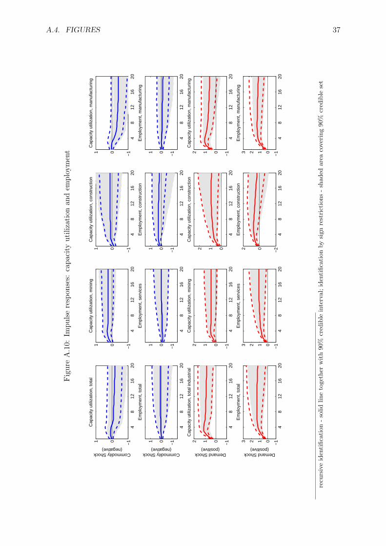
A.4. FIGURES 37
Fig
ure
A.1
0:Im
puls
ere
spon
ses:
capac
ity
uti
liza
tion
and
emplo
ym
ent
48
1216
20−
101C
apac
ity u
tiliz
atio
n, to
tal
Commodity Shock(negative)
48
1216
20−
101C
apac
ity u
tiliz
atio
n, m
inin
g
48
1216
20−
101C
apac
ity u
tiliz
atio
n, c
onst
ruct
ion
48
1216
20−
101C
apac
ity u
tiliz
atio
n, m
anuf
actu
ring
48
1216
20
−101
Em
ploy
men
t, to
tal
Commodity Shock(negative)
48
1216
20
−101
Em
ploy
men
t, se
rvic
es
48
1216
20
−101
Em
ploy
men
t, co
nstr
uctio
n
48
1216
20
−101
Em
ploy
men
t, m
anuf
actu
ring
48
1216
20−
1012C
apac
ity u
tiliz
atio
n, to
tal i
ndus
tria
l
Demand Shock(positive)
48
1216
20−
1012C
apac
ity u
tiliz
atio
n, m
inin
g
48
1216
20
012
Cap
acity
util
izat
ion,
con
stru
ctio
n
48
1216
20−
1012C
apac
ity u
tiliz
atio
n, m
anuf
actu
ring
48
1216
20−
10123E
mpl
oym
ent,
tota
l
Demand Shock(positive)
48
1216
20−
10123E
mpl
oym
ent,
serv
ices
48
1216
20−
202E
mpl
oym
ent,
cons
truc
tion
48
1216
20−
10123E
mpl
oym
ent,
man
ufac
turin
g
recu
rsiv
eid
enti
fica
tion
-so
lid
lin
eto
geth
erw
ith
90%
cred
ible
inte
rval
;id
enti
fica
tion
by
sign
rest
rict
ion
s-
shad
edar
eaco
veri
ng
90%
cred
ible
set

38 APPENDIX A. APPENDICES TO CHAPTER 1
Figu
reA
.11:Im
pulse
respon
ses:m
onetary
and
finan
cialin
dicators
48
1216
20−
0.5 0
0.5 1
1.5S
&P
/TS
X C
omposite Index
Commodity Shock(negative)
48
1216
20
−0.2 0
0.2
Bank rate
48
1216
20
−0.2 0
0.2
Treasury B
ill rate, 3 months
48
1216
20
−0.2 0
0.2 Governm
ent bonds rate, over 10 years
48
1216
20−
1 0 1 2M
onetary base
Commodity Shock(negative)
48
1216
20−
1 0 1 2 3M
onetary aggregate M3
48
1216
20−
1 0 1 2 3T
otal business credit
48
1216
20−
1 0 1T
otal foreign exchange reserves
48
1216
20−
0.5 0
0.5 1
1.5S
&P
/TS
X C
omposite Index
Demand Shock(positive)
48
1216
20
0
0.2
0.4B
ank rate
48
1216
20
0
0.2
0.4T
reasury Bill rate, 3 m
onths
48
1216
20
0
0.2
0.4 Governm
ent bonds rate, over 10 years
48
1216
20−
1 0 1 2M
onetary base
Demand Shock(positive)
48
1216
20
0 2 4M
onetary aggregate M3
48
1216
20
0 2 4T
otal business credit
48
1216
20−
1 0 1T
otal foreign exchange reserves
recursiv e
iden
tification
-solid
line
together
with
90%cred
ible
interval;
iden
tification
by
signrestriction
s-
shad
edarea
covering
90%cred
ible
set

A.5. TABLES 39
A.5 Tables

40 APPENDIX A. APPENDICES TO CHAPTER 1
Tab
leA
.2:Sectoral
comp
ositionof
the
Can
adian
econom
y:
averagesh
aresover
1985-2007
Gross
Valu
eA
dded
Em
ploy
men
tE
xp
ort(%
ofth
eN
etex
port
(%of
totalG
DP
)(%
oftotal
employ
men
t)in
dustry
pro
duction
)(%
oftotal
GD
P)
Prim
aryC
omm
odityS
ector7.7
4.836.1
2.8A
gricultu
re,forestry
and
fish
ing
2.63.7
23.00.6
Min
ing
and
quarry
ing
5.11.1
45.92.2
Tradable
Sector
17.514.6
46.9-0.7
Man
ufactu
ring
17.514.6
46.9-0.7
Non
-tradableS
ector74.7
80.54.3
-1.0U
tilities3.0
0.85.1
0.1C
onstru
ction5.8
6.1-
-Serv
ices65.9
73.74.8
-1.1
Data
:O
EC
DS
TA
Nd
atabase,
CA
NS
IMC
anad
a,av
erageover
1985-2007
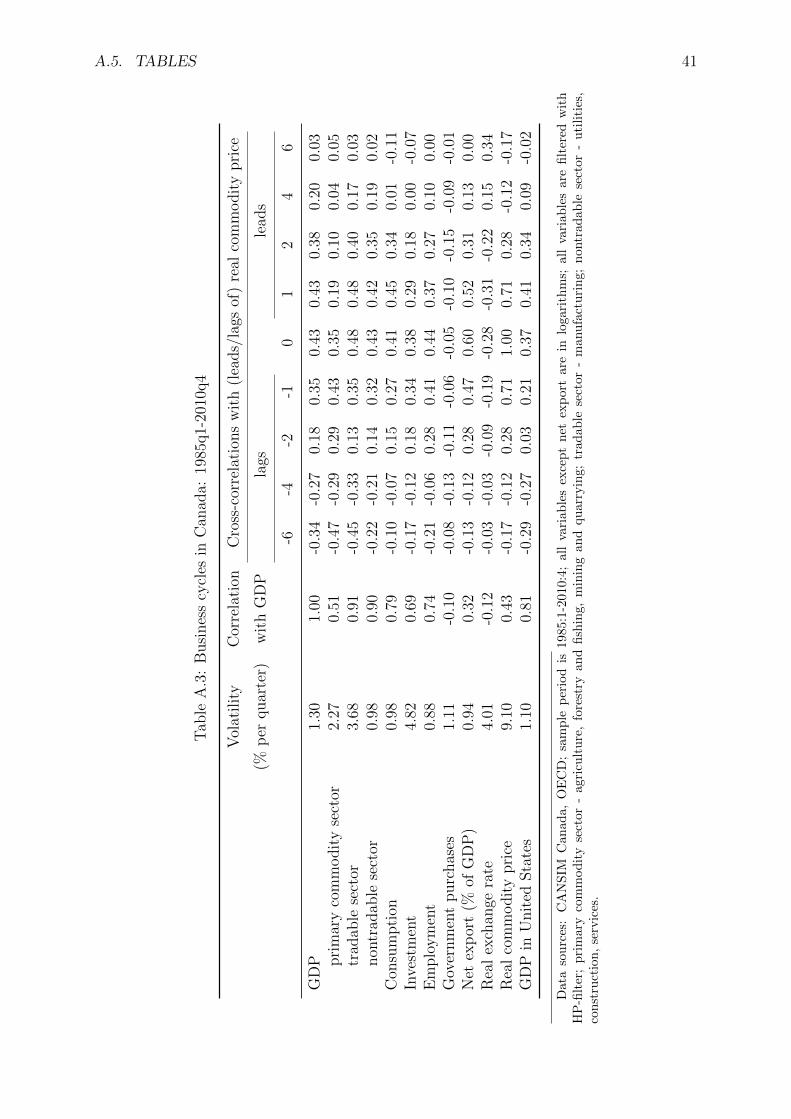
A.5. TABLES 41
Tab
leA
.3:
Busi
nes
scy
cles
inC
anad
a:19
85q1-
2010
q4
Vol
atilit
yC
orre
lati
onC
ross
-cor
rela
tion
sw
ith
(lea
ds/
lags
of)
real
com
modit
ypri
ce
(%p
erquar
ter)
wit
hG
DP
lags
lead
s
-6-4
-2-1
01
24
6
GD
P1.
301.
00-0
.34
-0.2
70.
180.
350.
430.
430.
380.
200.
03pri
mar
yco
mm
odit
yse
ctor
2.27
0.51
-0.4
7-0
.29
0.29
0.43
0.35
0.19
0.10
0.04
0.05
trad
able
sect
or3.
680.
91-0
.45
-0.3
30.
130.
350.
480.
480.
400.
170.
03non
trad
able
sect
or0.
980.
90-0
.22
-0.2
10.
140.
320.
430.
420.
350.
190.
02C
onsu
mpti
on0.
980.
79-0
.10
-0.0
70.
150.
270.
410.
450.
340.
01-0
.11
Inve
stm
ent
4.82
0.69
-0.1
7-0
.12
0.18
0.34
0.38
0.29
0.18
0.00
-0.0
7E
mplo
ym
ent
0.88
0.74
-0.2
1-0
.06
0.28
0.41
0.44
0.37
0.27
0.10
0.00
Gov
ernm
ent
purc
has
es1.
11-0
.10
-0.0
8-0
.13
-0.1
1-0
.06
-0.0
5-0
.10
-0.1
5-0
.09
-0.0
1N
etex
por
t(%
ofG
DP
)0.
940.
32-0
.13
-0.1
20.
280.
470.
600.
520.
310.
130.
00R
eal
exch
ange
rate
4.01
-0.1
2-0
.03
-0.0
3-0
.09
-0.1
9-0
.28
-0.3
1-0
.22
0.15
0.34
Rea
lco
mm
odit
ypri
ce9.
100.
43-0
.17
-0.1
20.
280.
711.
000.
710.
28-0
.12
-0.1
7G
DP
inU
nit
edSta
tes
1.10
0.81
-0.2
9-0
.27
0.03
0.21
0.37
0.41
0.34
0.09
-0.0
2
Dat
aso
urc
es:
CA
NS
IMC
anad
a,O
EC
D;
sam
ple
per
iod
is19
85:1
-201
0:4;
all
vari
able
sex
cep
tn
etex
por
tar
ein
loga
rith
ms;
all
vari
able
sar
efi
lter
edw
ith
HP
-filt
er;
pri
mar
yco
mm
od
ity
sect
or
-ag
ricu
ltu
re,
fore
stry
and
fish
ing,
min
ing
and
qu
arry
ing;
trad
able
sect
or-
man
ufa
ctu
rin
g;n
ontr
adab
lese
ctor
-u
tili
ties
,co
nst
ruct
ion
,se
rvic
es.

42 APPENDIX A. APPENDICES TO CHAPTER 1
Chapter 2
Commodity price shocks and real
business cycles in a small
commodity-exporting economy
2.1 Introduction
The share of primary commodities in world output and trade has declined over the last
century. Nevertheless, fluctuations in commodity prices still significantly affect economic
activity, especially in countries, where primary commodities remain a main source of
export earnings. In these countries commodity price movements have enormous impacts
on real output, exchange rates, balance of payments and public finance, and, as a result,
pose serious problems for the conduct of macroeconomic policy.
The economic literature emphasizes several important stylized facts regarding the ef-
fects of commodity price changes on business cycles in commodity-exporting economies.
These facts have been described in detail in Chapter 1 and can be summarized here as fol-
lows. First, real commodity prices are positively correlated with trade and current account
balances (external balances effect). Second, real exchange rates are highly volatile and
exhibit a negative correlation with the real commodity price, so that increasing commod-
ity price results in an appreciation of the real exchange rate (commodity currency effect).
Third, relative consumption between commodity-exporting economy and its trade part-
ners is negatively correlated with the real exchange rate, invalidating predictions of the
many international business cycles models with perfect financial markets (Backus-Smith
puzzle). Fourth, an increase in commodity export revenues is associated with a decline
in the non-commodity tradable sector (Dutch disease). And, finally, there is a positive
effect of the real commodity price on investment (investment effect).
A range of the models have been proposed in the economic literature to explain the
effects of the world commodity price (and/or terms-of-trade) shocks on business cycles
43

44 CHAPTER 2. RBC IN A SMALL COMMODITY-EXPORTING ECONOMY
in a small commodity-exporting economy, starting from the early deterministic analysis
of Dutch disease in Corden and Neary (1982) and Bruno and Sachs (1982). So, for
example, Mendoza (1995) analyses the quantitative importance of terms of trade shocks
in driving business cycles using a dynamic stochastic small open economy model. Kose
(2002) extends Mendoza’s work by developing a richer production structure that captures
several empirically relevant features of developing economies. Sosunov and Zamulin (2007)
and Dib (2008) study monetary policy in resource rich economies, in application to Russia
and Canada respectively. These recent models are constructed in the line with new open
economy macroeconomics paradigm and feature a small open economy structure, multiply
goods, exogenous world commodity price shocks and one non-risky internationally traded
asset. However, they have several drawbacks.
First, the world economy is often not modeled explicitly. The foreign variables, such
as real commodity price, terms of trade, world interest rate and world output, are usu-
ally introduced as exogenous stochastic shocks. Interrelations between these extraneous
variables are either imposed using the variance-covariance matrix or not specified at all.
However, this approach may be misleading, given that the world prices and interest rates
are not shocks per se. These variables reflect endogenous responses of the world economy
to many distinct supply and demand shocks. As it has been shown in Chapter 1, despite
some of these world-wide shocks increase commodity prices, their overall effects on a small
commodity-exporting economy may be completely different.
Second, in these models there is usually only one non-risky internationally traded as-
set. However, an assumption of incomplete markets in a stochastic small open economy
model results in steady-state equilibrium that depends on initial conditions and equilib-
rium dynamics that possess a random walk component. To induce a stationarity standard
models usually assume non-separable preferences or some form of frictions in assets trade
(Schmitt-Grohe and Uribe, 2003). But these additional elements, without an assump-
tion of incomplete markets itself, may be responsible for generating many stylized facts
in aforementioned models. Indeed, as Chari, Kehoe, and McGrattan (2002) show, the
models with incomplete markets and without other frictions fail to solve Backus-Smith
and exchange rate volatility puzzles. Besides, their dynamics is close to those generated
by the models with complete markets.1 So, an assumption of incomplete markets is not
very crucial and working with complete markets may be more convenient.
In this chapter I propose a new real business cycles model of a small commodity-
exporting economy explaining simultaneously the five stylized facts regarding this econ-
omy. In contrast to the existing literature, the foreign (world) economy is modeled ex-
1Benigno and Thoenissen (2007) show that a model with incomplete markets and nontradable inter-mediate goods can solve Backus-Smith puzzle, though it fails to generate volatile real exchange rate.Therefore, in this chapter I report also impulse responses for the model with incomplete markets. Sim-ulations show that dynamics of this model are very close to those in the model with complete markets.That is in the line with results of Chari et al. (2002).

2.1. INTRODUCTION 45
plicitly, so all the world prices are determined endogenously in response to the global
productivity and commodity endowment shocks. That allows also to control explicitly
cross-country risk-sharing. The only key difference between home and foreign economies
is in different productivity levels in tradable, nontradable and commodity sectors, such
that home economy appears to be relatively abundant in primary commodities.
In the initial version of the model I assume complete assets markets and no frictions
in intertemporal trade. This model generates a positive correlation between commodity
price and trade balance, but cannot reproduce volatile and negatively correlated with
the real commodity price real exchange rate. Moreover, relative consumption moves in
lockstep with the real exchange rate, illustrating Backus-Smith puzzle. In this model
international risk sharing is working well and frictions in intratemporal trade are not high
enough to induce significant volatility in the real exchange rate. Besides, in this model
there is no manifestation of Dutch disease and investment effect.
Next, the opposite case will be considered, when home country has no access to finan-
cial markets but intratemporal trade is allowed (financial autarky). Because international
risk sharing via trade in financial assets is not possible, commodity price shocks induce
very volatile real exchange rate, which is negatively correlated with commodity prices
and relative consumption. This model also predicts Dutch disease and investment effect.
Nevertheless, assumption of financial autarky is too strict and contradicts observable
fluctuations in trade balances.
To increase a volatility of the real exchange rate and to damp risk sharing in the
model with complete markets I need to break link between marginal rate of substitution
in consumption across countries and real exchange rate. There are several ways to do it.
The first approach is to introduce occasionally binding borrowing constraints. These
constraints may be exogenous, given, for example, by the rule which prevents country
to borrow or save beyond some limits. It is possible also to model these constraints
endogenously, assuming a limited enforcement of international contracts, as in Alvarez
and Jermann (2000), Kehoe and Perri (2002) and Bodenstein (2008).2
The second strategy is to assume some kind of frictions in assets trade. For example,
agents may face convex costs of holding assets in quantities different from some long-run
level as in (Schmitt-Grohe and Uribe, 2003).3
2In the model of a small open economy two-sided limited commitment is not possible, because thevalue of autarky for foreign economy coincides with the value of intertemporal trade. The case of one-sided limited commitment is not very interesting, since small economy can effectively achieve risk sharingunder full commitment by accumulating assets, which would be seized in the case of default (see Itskhoki,2007).
3An alternative way to break link between relative consumption and real exchange rate and to in-crease volatility of the real exchange rate without introduction of frictions in assets trade is to relax anassumption of additive separable preferences. Nonseparable preferences create wedge between relativeconsumption and cross-country marginal rate of substitution of consumption, though the latter is stillequal to the real exchange rate. For example, Verdelhan (2010) discusses this effect using habit-basedpreferences.

46 CHAPTER 2. RBC IN A SMALL COMMODITY-EXPORTING ECONOMY
The last strategy is applied in this chapter. To adjust the value of portfolio of interna-
tional assets, the home households have to bear transaction costs. This model succeeded
to replicate all aforementioned stylized facts about commodity-exporting economies.
The rest of the chapter is organized as follows. Section 2 provides an empirical evidence
regarding the effects of the real commodity price changes on business cycles in selected
commodity-exporting countries. Section 3 presents the model of a small commodity-
exporting economy. Section 4 discusses calibration and computational algorithm. Section
5 reports the main results. Section 6 concludes.
2.2 An empirical evidence
In this section, I briefly discuss an empirical evidence about business cycles in selected
commodity-exporting countries. I focus here on four developed resource rich countries,
data of which are abundant: Australia, Canada, Norway and New Zealand.4
Figures B.1-B.2 illustrate some stylized facts regarding business cycles in these coun-
tries. The upper part of these figures shows a relationship between the effective real
exchange rate and relative consumption.5 The middle part illustrates dynamics of the
real commodity price6 and the effective real exchange rate. And finally, the lowest part
shows the trade balance (as share of GDP) and the real commodity price index. Table B.1
summarizes the second moments of data for these countries, computed both for the levels
and for the HP-filtered series. Data are presented both for the period of 1970-2008 and
for the less turbulent sub-period of 1985-2008. In what follows, I will discuss the results
for the HP-filtered series.
As the table shows, the real commodity price index is very volatile. Its standard devi-
ation varies from 7.95% in New Zealand to 14.16% in Norway. The effective real exchange
rates are also highly volatile and negatively correlated with the real commodity prices,
illustrating the commodity currency effect. This negative correlation is more apparent for
the recent period of 1985-2008 and is more pronounced for Australia and New Zealand.
These countries also manifest the highest standard deviations of the real exchange rate.
The real commodity prices are positively correlated with trade balance (at least for
the period of 1985-2008) and investment (except of Norway). The data illustrate appar-
4According to the UN COMTRADE database, top three exported primary commodities (two-digits)in 2007 for these countries were as follows (a share in total export is reported). Canada: petroleum,petroleum products and related materials - 12.5%, gas, natural and manufactured - 7%, non-ferrousmetals - 5.4%. Australia: metalliferous ores and metal scrap - 20.5%, coal, coke and briquettes - 12.4%,non-ferrous metals - 8.1%. Norway: petroleum, petroleum products and related materials - 44.6%, gas,natural and manufactured - 19.3%, non-ferrous metals - 7.7%. New Zealand: dairy products and birds’eggs - 20.6%, meat and meat preparations - 12.1%, vegetables and fruit - 5.3%.
5Relative consumption is computed against the country or block of countries with the highest shareof mutual trade: Canada vs. US, Australia vs. OECD, Norway vs. EU and New Zealand vs. Australia.
6The real commodity price is computed as a price index of exported primary commodities (in USdollars) deflated by the consumer price index in the United States.

2.3. THE MODEL 47
ently the Backus-Smith puzzle. Moreover, for Canada, Australia and New Zealand the
correlation between the real exchange rate and relative consumption is negative for the
recent data.
The most interesting pattern is shown by the Norway’s data. Though the real com-
modity price index in this country is the most volatile in my sample, its effective real
exchange rate has the lowest standard deviation.7 Besides, a negative correlation between
the real exchange rate and commodity prices is not very strong, -0.14, comparing to -0.41
in Australia. Investment in Norway is negatively correlated with the real commodity price
index, which is in contrast to other developed commodity-exporting countries where this
correlation is positive. Trade balance is closely linked with the real commodity price.
Consumption differential with the EU is not correlated with the real exchange rate. In
addition, for the most recent data this correlation is positive, that is closer to unitary
value predicted by the international business cycle models with perfect financial mar-
kets. As this chapter shows, all these facts may indicate about the better functioning
of international risk sharing in Norway comparing to other countries considered in this
section.
2.3 The model
This section presents a real business cycle model of a small commodity-exporting economy.
The model is introduced in three steps. First, I discuss a general theoretical framework
for modeling the world economy as a continuum of small open economies. Then, specific
assumptions about productivities and commodity endowments will be made to reduce this
general model to the more tractable two-country model, where the first region corresponds
to a small commodity-exporting economy whereas the second one to the global economy
as a whole. And, finally, I will discuss three alternative variants of this simplified model
under the different assumptions about the extent of risk-sharing between these two regions,
namely i) the model with complete markets, ii) the model of financial autarky and iii) the
model with financial transaction costs.
Notation is as follows. Variables with an i subscript refer to economy i, one among
the continuum of economies making up the world economy. Variables without an i-index
denote a small commodity-exporting economy being modelled. Finally, variables with a
star superscript correspond to the world economy as a whole (typical foreign economy).
7Norway exports mainly energy resources, prices of which are the most volatile among the primarycommodities.

48 CHAPTER 2. RBC IN A SMALL COMMODITY-EXPORTING ECONOMY
2.3.1 General description of the model
The world economy is modeled as a continuum of small open economies represented by
unit interval, as in Gali and Monacelli (2005). All economies have the same preferences,
technology and market structure. Assets markets are complete.
A typical small economy produces three types of good: differentiated tradable good,
differentiated nontradable good and homogeneous primary commodity. Tradable goods
can be used for consumption and investment either in domestic economy or abroad,
whereas nontradable goods can be invested or consumed only in domestic country. Com-
modity can be consumed, exported or used along with labor and capital as an input in
production of tradable and nontradable goods. The firms producing tradable and non-
tradable goods and commodity endowments are owned by the domestic households.
The world economy is affected by the productivity shocks in tradable and nontradable
sectors as well as by the commodity endowments shocks.
2.3.2 Households
A typical small economy i is inhabited by representative household, which maximizes
expected life-time utility:
maxct,lt,at+1
E0
∞∑t=0
βtU (ct(i), 1− lt(i)) (2.1)
subject to a sequence of budget constraints expressed in units of domestic consumption
good:
ct(i) +
∫st+1
qt,t+1(st+1, i)at+1(st+1, i)dst+1 ≤ at(i) + wt(i)lt(i) + Πt(i) (2.2)
where ct is a composite consumption good, lt denotes hours worked, wt is a real wage,
at+1 are holdings of the Arrow-Debreu securities, priced at qt,t+1, Πt denotes profits from
the domestic firms and commodity endowment. All prices are given in terms of domestic
consumption and can be converted into prices in terms of consumption in country j trough
division by bilateral real exchange rate et(i, j) (the price of consumption good in j in terms
of consumption in country i).8 The problem is supplemented with a natural borrowing
constraint to avoid Ponzi schemes.
The composite consumption good ct is a CES basket of the tradable cT,t, nontradable
8So, an increase in bilateral real exchange rate et(i, j) reflects depreciation of the real exchange ratein country i and respectively its appreciation in country j. No arbitrage implies that et(i, j) = et(j, i)
−1
and et(i, j)et(j, k) = et(i, k).

2.3. THE MODEL 49
cN,t goods and commodity cX,t:
ct(i) =(α
1εCT c
ε−1ε
T,t (i) + α1εCNc
ε−1ε
N,t (i) + (1− αCT − αCN)1ε c
ε−1ε
X,t (i)) εε−1
(2.3)
where ε denotes an elasticity of substitution between tradable and nontradable goods
(with ε < 1) and αCT and αCN reflect the weights of tradable and nontradable goods in
composite index.
The index of tradable goods cT,t is in turn a CES basket of the home cH,t and foreign
cF,t tradable goods:
cT,t(i) =(α
1θCHc
θ−1θ
H,t (i) + (1− αCH)1θ c
θ−1θ
F,t (i)) θθ−1
(2.4)
where θ is an elasticity of substitution between home and foreign tradable goods (with
ε < θ) and αCH reflects the home bias in consumption of tradable goods.
Foreign tradable good cF,t is an aggregate of all imported tradable goods:
cF,t(i) =
(∫ 1
0
cθ−1θ
F,t (i, j)dj
) θθ−1
(2.5)
Households allocate their consumption by solving expenditure minimization problem
(taking prices of goods as given).
2.3.3 Firms
The markets for all goods in the model are perfectly competitive. All the firms and
commodity endowments are assumed to be owned by domestic households. Technology
in tradable and nontradable sectors is symmetric across the world.
A typical firm producing nontradable good has the following production function:
yN,t(i) =
((1− φN)
1ξ
(AN,t(i)k
βNKN,t (i)l1−βNKN,t (i)
) ξ−1ξ
+ φ1ξ
Nxξ−1ξ
N,t (i)
) ξξ−1
(2.6)
where AN,t is a productivity in the nontradable sector, kN,t, lN,t and xN,t are capital, labor
and commodity inputs, ξ is elasticity of substitution between value added and commodity
input and φN denotes share of commodity input in the total costs of nontradable firm.
This firm maximizes the expected discounted value of profits:
maxkN,t+1,lN,t,xN,t,i
dN,t
E0
∞∑t=0
βtUc (ct(i), 1− lt(i))Uc (c0(i), 1− l0(i))
ΠN,t(i) (2.7)

50 CHAPTER 2. RBC IN A SMALL COMMODITY-EXPORTING ECONOMY
with profits ΠN,t determined as:
ΠN,t(i) = pN,t(i)yN,t(i)− pI,t(i)idN,t(i)− wt(i)lN,t(i)− pX,t(i)xN,t(i) (2.8)
where pN,t, pI,t and pX,t denote prices of nontradable good, investment and commodity
respectively.
Maximization is subject to constraints imposed by the production function (2.6) and
by the following capital transition equation:
kN,t+1(i) = (1− δ)kN,t(i) + kN,t(i)Ψk
(idN,t(i)
kN,t(i)
)(2.9)
where δ is depreciation rate and idN,t denotes new investment into nontradable sector
with installation costs determined by function Ψk (·).9 The capital adjustment costs are
introduced into this model to avoid excessive equilibrium volatility of investment. An
initial capital stock in nontradable sector kN,0(i) is given.
A typical firm in tradable sector solves a similar problem. It maximizes the expected
discounted value of lifetime profits:
maxkT,t+1,lT,t,xT,t,i
dT,t
E0
∞∑t=0
βtUc (ct(i), 1− lt(i))Uc (c0(i), 1− l0(i))
ΠT,t(i) (2.10)
with profits ΠT,t determined as:
ΠT,t(i) = pH,t(i)yT,t(i)− pI,t(i)idT,t(i)− wt(i)lT,t(i)− pX,t(i)xT,t(i) (2.11)
where kT,t, lT,t and xT,t are capital, labor and commodity inputs and pH,t is price of
domestic tradable good.
Maximization is constrained by the production function and capital transition equa-
tion:
yT,t(i) =
((1− φT )
1ξ
(AT,t(i)k
βTKT,t (i)l1−βTKT,t (i)
) ξ−1ξ
+ φ1ξ
Txξ−1ξ
T,t (i)
) ξξ−1
(2.12)
kT,t+1(i) = (1− δ)kT,t(i) + kT,t(i)Ψk
(idT,t(i)
kT,t(i)
)(2.13)
where AT,t is a productivity in the tradable sector, φT is share of commodity input in
total costs of tradable firm, δ is depreciation rate and idT,t denotes new investment into
tradable sector with installation costs Ψk (·). An initial capital stock in tradable sector
kT,0(i) is given.
9Capital adjustment costs function Ψk (·) has to satisfy the following properties in the steady state:Ψk (δ) = δ, Ψ′k (δ) = 1 and Ψ′′k (δ) = d < 0.

2.3. THE MODEL 51
Investment good it is a CES basket of the tradable iT,t and non-tradable iN,t goods:
it(i) =(α
1εIT i
ε−1ε
T,t (i) + (1− αIT )1ε i
ε−1ε
N,t (i)) εε−1
(2.14)
where αIT reflects the weight of tradable goods in composite investment index. It is as-
sumed that the share of tradable goods in investment is higher comparing to consumption,
so αITαCT
> αINαCN
with αIN = 1− αIT .
Investment expenditure on tradable goods iT,t is a CES basket of the home iH,t and
foreign iF,t tradable goods:
iT,t(i) =(α
1θIHi
θ−1θ
H,t (i) + (1− αIH)1θ i
θ−1θ
F,t (i)) θθ−1
(2.15)
where
iF,t(i) =
(∫ 1
0
iθ−1θ
F,t (i, j)dj
) θθ−1
(2.16)
Firms allocate their investment demand by solving expenditure minimization problem
(taking prices of goods as given).
Production in commodity sector is exogenously determined and does not incur any
costs. Therefore, the profits of this sector are product of commodity endowment Xt and
its price pX,t:
ΠX,t(i) = pX,t(i)Xt(i) (2.17)
Total profits from the nontradable, tradable and commodity sectors are distributed across
domestic households, so:
Πt(i) = ΠN,t(i) + ΠT,t(i) + ΠX,t(i) (2.18)
2.3.4 Market clearing conditions
All goods, factors and assets markets clear at any time and any contingency.
Markets of tradable and nontradable goods:
yN,t(i) = cN,t(i) + iN,t(i),∀i, t (2.19)
yT,t(i) = cH,t(i) +
∫ 1
0
cF,t(j, i)dj + iH,t(i) +
∫ 1
0
iF,t(j, i)dj, ∀i, t (2.20)
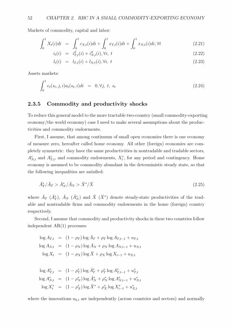
52 CHAPTER 2. RBC IN A SMALL COMMODITY-EXPORTING ECONOMY
Markets of commodity, capital and labor:∫ 1
0
Xt(i)di =
∫ 1
0
cX,t(i)di+
∫ 1
0
xT,t(i)di+
∫ 1
0
xN,t(i)di, ∀t (2.21)
it(i) = idT,t(i) + idN,t(i),∀i, t (2.22)
lt(i) = lT,t(i) + lN,t(i),∀i, t (2.23)
Assets markets:∫ 1
0
et(st, j, i)at(st, i)di = 0, ∀j, t, st (2.24)
2.3.5 Commodity and productivity shocks
To reduce this general model to the more tractable two-country (small commodity-exporting
economy/the world economy) case I need to make several assumptions about the produc-
tivities and commodity endowments.
First, I assume, that among continuum of small open economies there is one economy
of measure zero, hereafter called home economy. All other (foreign) economies are com-
pletely symmetric: they have the same productivities in nontradable and tradable sectors,
A∗N,t and A∗T,t, and commodity endowments, X∗t , for any period and contingency. Home
economy is assumed to be commodity abundant in the deterministic steady state, so that
the following inequalities are satisfied:
A∗T/AT > A∗N/AN > X∗/X (2.25)
where AT (A∗T ), AN (A∗N) and X (X∗) denote steady-state productivities of the trad-
able and nontradable firms and commodity endowments in the home (foreign) country
respectively.
Second, I assume that commodity and productivity shocks in these two countries follow
independent AR(1) processes:
logAT,t = (1− ρT ) log AT + ρT logAT,t−1 + uT,t
logAN,t = (1− ρN) log AN + ρN logAN,t−1 + uN,t
logXt = (1− ρX) log X + ρX logXt−1 + uX,t
logA∗T,t = (1− ρ∗T ) log A∗T + ρ∗T logA∗T,t−1 + u∗T,t
logA∗N,t = (1− ρ∗N) log A∗N + ρ∗N logA∗N,t−1 + u∗N,t
logX∗t = (1− ρ∗X) log X∗ + ρ∗X logX∗t−1 + u∗X,t
where the innovations uk,t are independently (across countries and sectors) and normally

2.3. THE MODEL 53
distributed.
Since the home economy has measure zero it does not affect an equilibrium in the
foreign economies. A symmetry across the last ones implies in turn a symmetry of their
equilibrium allocations and prices.10 So, I can treat a typical foreign economy as the
world economy at whole.
To compute an equilibrium of this model I will proceed in two steps. Initially, I com-
pute an equilibrium of the world economy (representative foreign economy). It provides
us with the world prices of commodity p∗X,t, foreign tradable good p∗T,t and Arrow-Debreu
securities q∗t,t+1 as well as with the foreign demands on tradable consumption c∗T,t and trad-
able investment i∗T,t. These prices and allocations are contingent on foreign productivity
and commodity shocks A∗T,t, A∗N,t and X∗t . An equilibrium in the home economy is com-
puted in the second stage, taking the world demand and prices as given. All equilibrium
conditions of the model are given in Appendix B.
2.3.6 Model with complete assets markets
Under the assumptions of complete markets and frictionless assets trade, the first-order
optimal conditions for the home and foreign representative households imply that:
et+1
et
Uc (ct+1, 1− lt+1)
Uc (ct, 1− lt)=Uc(c∗t+1, 1− l∗t+1
)Uc (c∗t , 1− l∗t )
(2.26)
Therefore,
etUc (ct, 1− lt) = ϑ0Uc (c∗t , 1− l∗t ) (2.27)
where ϑ0 is constant for all periods and contingencies and reflects an initial wealth position
of the home economy comparing to the foreign one.
It means, that given the correction for wealth differences, a marginal rate of substi-
tution between home and foreign consumption has to be equal to their relative price, i.e.
the real exchange rate. In other words, other things being equal, consumption is higher
in the country where its price, converted into a common currency, is lower.11 It is in
contrast to empirical evidence, which suggests that there are no any systematic comove-
ment between relative consumption and real exchange rate. This collusion is well known
10In particular, symmetric equilibrium in the world economy implies that cF,t(i) = cF,t(i, j) = c∗F,t,iF,t(i) = iF,t(i, j) = i∗F,t, pT,t(i) = pH,t(i) = pF,t(i) = p∗T,t and, consequently, cT,t(i) = cH,t(i) + cF,t(i) =c∗T,t and iT,t(i) = iH,t(i) + iF,t(i) = i∗T,t for all foreign economies i and j. So, in the equilibriumdifferentiated foreign tradable goods can be treated as one homogeneous foreign tradable good. Besides,equilibrium financial asset holdings of the foreign economy are null for any period and contingency:at(i) = 0.
11Non-separability of consumption and leisure in utility implies that correlation between relative con-sumption and real exchange rate is not perfect in contrast to correlation between cross-country marginalrate of substitution and real exchange rate. Nevertheless, the simulation results show that this effect isnegligible.
54 CHAPTER 2. RBC IN A SMALL COMMODITY-EXPORTING ECONOMY
in the economic literature and is called a consumption-real exchange rate anomaly or a
Backus-Smith puzzle (Backus and Smith, 1993).
It should be emphasized, that condition (2.27) does not imply in general a perfect
international risk-sharing, understood as a lock-step comovement of consumption across
countries in response to productivity and commodity shocks. As Brandt, Cochrane, and
Santa-Clara (2006) stress, a risk sharing requires also frictionless goods markets. They
argue:
Suppose that Earth trades assets with Mars by radio, in complete and fric-
tionless capital markets. If Mars enjoys a positive shock, Earth-based owners
of Martian assets rejoice in anticipation of their payoffs. But trade with Mars
is still impossible, so the real exchange rate between Mars and Earth must
adjust exactly to offset any net payoff. In the end, Earth marginal utility
growth must reflect Earth resources, and the same for Mars. Risk sharing is
impossible. If the underlying shocks are uncorrelated, the exchange rate vari-
ance is the sum of the variances of Earth and Mars marginal utility growth,
and I measure a zero risk sharing index despite perfect capital markets... At
the other extreme, if there is costless trade between the two planets (teletrans-
portation), and the real exchange rate is therefore constant, marginal utilities
can move in lockstep. With constant exchange rates, I measure a perfect risk
sharing index of one.
In my model there are nontradable goods. Besides, consumption of tradable goods,
which are not perfect substitutes across countries, is home-biased. So, the productivity
shocks in tradable and nontradable sectors cannot be perfectly insured and result in
volatile real exchange rate. Non-separability of consumption and leisure in utility together
with nontradable labor imply some degree of real exchange rate volatility too.
2.3.7 Model of financial autarky
In the model with complete markets, an international risk sharing is not too bad despite
the presence of frictions in international trade. In other words, these frictions are not
sufficient to induce an observed high volatility of the real exchange rate in commodity-
exporting economies. International capital markets are prefect and provide enough insur-
ance against productivity and commodity shocks.
Now, in contrast, I assume that international financial markets disappeared and the
home economy has no access to international borrowing and saving, but is allowed to
trade intratemporally. This is the case of financial autarky, which, to some extent, is
opposite to the model with complete markets.
The home representative household in this model maximizes its expected life-time

2.3. THE MODEL 55
utility subject to a new sequence of budget constraints:
ct ≤ wtlt + Πt (2.28)
where ct is a composite consumption good, lt denotes hours worked, wt is a real wage and
Πt denotes profits from the home firms and endowment.
The foreign representative household’s problem, problems of the firms and market
clearing conditions (except of the absent assets markets) are analogous to the previous
case. As in the model with complete markets, the world prices are completely determined
in the equilibrium for the world economy. The equilibrium conditions for this model are
reported in Appendix B.
The law of one price for financial assets and consequently condition (2.27) are not
satisfied in the model of financial autarky. Instead, an equilibrium in the home economy
is determined by the balanced trade condition:
tbt = pH,t(c∗H,t + i∗H,t) + pX,t(X − cX,t − xT,t − xN,t)− pF,t(cF,t + iF,t) = 0 (2.29)
where pH,t(c∗H,t + i∗H,t) and pX,t(X − cX,t − xT,t − xN,t) are exports respectively of home
tradable goods and commodity, whereas pF,t(cF,t + iF,t) is import of foreign tradables.
To compare this model with the complete markets case it would be useful to compute
the time and state-varying variable ϑt reflecting the wedge between the cross-country
marginal rate of substitution of consumption and the real exchange rate:
etUc (ct, 1− lt) = ϑtUc (c∗t , 1− l∗t ) (2.30)
This wedge induces an additional volatility in the real exchange rate and solves the
Backus-Smith puzzle, breaking the link between relative consumption and real exchange
rate. Nevertheless, financial autarky is a too restrictive assumption. So, it would be
interesting to consider an intermediate case, where the home country can borrow and
save abroad but there are frictions in financial assets trade.
2.3.8 Model with portfolio adjustment costs
Now I assume, that when adjusting the portfolio of international assets the agents bear
transaction costs. Home representative household in this model maximizes expected life-
time utility subject to a modified sequence of budget constraints:
ct +
∫st+1
qt,t+1(st+1, i)at+1(st+1, i)dst+1+
+ pN,tΨa
(∫st+1
qt,t+1(st+1, i)at+1(st+1, i)dst+1 − at)≤ at + wtlt + Πt
(2.31)

56 CHAPTER 2. RBC IN A SMALL COMMODITY-EXPORTING ECONOMY
where ct is a composite consumption good, lt denotes hours worked, wt is a real wage,
at+1 denotes portfolio of Arrow-Debreu securities priced at qt,t+1, Ψa(·) are portfolio ad-
justment costs and Πt are profits. I assume that all portfolio adjustment costs are paid
in nontradable goods and Ψa(·) is a convex function satisfying the following properties:
Ψa(z) ≥ 0 and Ψa(z) = 0 if and only if z = 0, zΨ′a(z) ≥ 0 and Ψ′′a(z) > 0.12
The foreign representative household’s problem, problems for the firms and market
clearing conditions are the same as in the complete markets model.13
The first order intertemporal optimal condition for the representative household is
given by:
qt,t+1 = βUc (ct+1, 1− lt+1)
Uc (ct, 1− lt)1 + pN,t+1Ψ
′a,t+1
1 + pN,tΨ′a,t(2.32)
where Ψ′a,t = Ψ′a (tbt).
This condition implies that:
etUc (ct, 1− lt) = ϑtUc (c∗t , 1− l∗t ) (2.33)
where
ϑt =ϑ0
1 + pN,tΨ′a(tbt)(2.34)
So, in this model there is a wedge between cross-country marginal rate of substitution
and the real exchange rate. This wedge implies a negative correlation between the real
exchange rate and the world commodity prices. Indeed, negative commodity shock in
the foreign economy results in commodity price growth and trade balance surplus. Since
ϑt is a decreasing function of the trade balance, the real exchange rate have to decrease
(appreciate).
Besides, this model generates an additional volatility in the real exchange rate and
solves the Backus-Smith puzzle. But, in contrast to the financial autarky, it allows inter-
national borrowings and savings.
2.4 Calibration
The model was calibrated to the Canadian economy, whereas the parameters of the world
economy were approximated using US data. The calibrated parameters are summarized
in Table B.2.
12These convex portfolio adjustment costs are somewhat ad hoc. However, the main aim of this chapteris not to explain a source of financial frictions, but to illustrate the effects of these frictions on businesscycles in a small commodity-exporting economy.
13Given that portfolio adjustment costs are paid in home nontradable good, the market clearing con-
dition for this good is now: yN,t = cN,t + iN,t + Ψa
(∫st+1
qt,t+1(st+1, i)at+1(st+1, i)dst+1 − at)
.

2.4. CALIBRATION 57
Table B.3 presents the breakdown of industries into commodity, tradable and non-
tradable sectors according to the International Standard Industrial Classification (ISIC,
Rev. 3). The commodity sector includes agriculture, mining and selected manufacturing
industries producing semi-processed raw materials (wood and pulp, metals, chemicals,
petroleum and coal products, etc.). The tradable sector consists of the rest of manufac-
turing (food and tobacco, textile, machinery and equipment manufacturing, etc.) and
internationally traded services (transport, financial intermediation, computer and other
business services). The nontradable sector includes the rest of services, public utilities
and construction.
2.4.1 Preferences and technology
The following functional form for the utility function is assumed in this chapter:
U (c, 1− l) =
(cγ (1− l)1−γ
)1−σ1− σ
This functional form implies that consumption and leisure are non-separable in utility.
The discount factor β is set to 0.99 to match 4% annual real rate in steady state. The
risk aversion parameter σ is equal to 2. The labor share γ is set to 0.38, so the fraction
of working time in steady state is 30%.
The elasticity of substitution in consumption between commodity, tradable and non-
tradable goods ε is set to 0.74 following Mendoza (1995). I assume that elasticity of substi-
tution between home and foreign tradable goods θ is equal to 1.5 as in Backus, Kehoe, and
Kydland (1992). The shares of tradable (aCT = 0.23) and nontradable (aCN = 0.73) goods
in consumption basket were computed using input-output data for Canada.14 The weight
of home tradable good in tradable consumption aCH is set to 0.68. The corresponding
shares for investment are aIT = 0.38 and aIH = 0.31. So, the weight of tradable goods in
investment is higher than in consumption. Besides, consumption of tradables in Canada
is home-biased, whereas investment expenditure on tradable goods goes predominantly
to import.
The shares of capital in the value added, bTK and bNK , are computed using input-
output data for Canada, found to be approximately the same across sectors and equal to
0.34. The weights of commodity input in total costs for tradable φT and nontradable φN
sectors are set to 20% and 10% respectively. So, the tradable sector uses commodity more
intensively than the nontradable one, what makes it more vulnerable to the commodity
price hikes. The elasticity of substitution between value added and commodity input ξ
is set to 0.69 for both sectors. That is in the line with the estimate of Rotemberg and
Woodford (1996). I assume also that the capital stocks in both sectors depreciate at the
14OECD Input-Output Database, 2006 edition.

58 CHAPTER 2. RBC IN A SMALL COMMODITY-EXPORTING ECONOMY
same rate of 2.5% per quarter.
The steady-state productivity levels in the foreign tradable A∗T and nontradable A∗Nsectors were computed, assuming that in the steady state all prices of foreign goods (in
terms of the foreign consumption) are equal to 1 and normalizing the steady-state foreign
commodity endowment X∗ to 1. Both values are found to be equal to 3.13. To compute
the productivity levels in tradable AT and nontradable AN sectors in the home country I
use the estimates of multi-factor productivity gap between US and Canada for different
industries, reported by Rao, Tang, and Wang (2004). According to these estimates the
productivity levels in Canada constitute 79% and 92% of those in US for tradable and
nontradable sectors respectively. Implied values of AT and AN are equal to 2.47 and 2.88.
It is assumed also that the home economy is commodity abundant, so in the steady state
X = 1.41.
Finally, we need to calibrate the stochastic processes describing productivity and com-
modity endowments shocks. The serial correlation coefficients are assumed to be sym-
metric across sectors and countries and equal to ρ = 0.8. The standard deviations of
innovations in tradable and nontradable sectors are set to satisfy proportion two to one
in both countries. The shocks to commodity endowments are assumed to be twice more
volatile than productivity shocks in tradable sector for the home economy and three times
more volatile for the foreign economy. These proportions correspond roughly to those
computed from the OECD data on labor productivity (see Table C.1 in Chapter 3).15
2.4.2 Capital and portfolio adjustment costs
The capital adjustment costs are symmetric across sectors and countries. The following
functional form is assumed in this chapter: Ψk(z) = ψ0+ψ1zψ2 . The parameters are set to
guarantee, that in the steady-state equilibrium Ψk(δ) = δ, Ψ′k(δ) = 1 and Ψ′′k(δ) = d < 0.
The value of d is chosen so as to ensure that a volatility of investment is three times higher
than that of GDP.
The portfolio adjustment costs function is Ψa(z) = ψz2. The parameter ψ is set so to
guarantee that a standard deviation of trade balance to GDP ratio is equal to 0.9, as in
the data for Canada.
2.4.3 Algorithm
The equilibrium conditions of the model are log-linearized around the deterministic steady
state. A corresponding system of linear expectational difference equations is solved by
generalized Schur decomposition (QZ) algorithm (see Klein, 2000; Sims, 2002) realized in
15Notice that (HP-filtered) labor productivity in the Canada’s commodity sector was less volatile in1980-2008 comparing to the OECD average and United States.

2.5. RESULTS 59
Dynare16 package.
2.5 Results
This section reports the steady-state solution and simulation results for the different
variants of the model of a small commodity-exporting economy.
2.5.1 Deterministic steady-state equilibrium
Given the cross-country asymmetries in the model, it would be interesting to consider its
deterministic steady-state equilibrium. It is assumed that both economies have balanced
trade in the steady state, so the corresponding equilibria are the same for all variants of
the model. The steady-state solution is presented in Table B.4. Several observations are
worth noting.
First, international trade flows fit well with the predictions of the comparative ad-
vantage theory. The home economy exports primary commodities whereas its import of
foreign tradable goods exceeds the export of home tradables. Moreover, the relative price
of domestic tradables to commodity in the home country is higher than abroad.
Second, production in the home economy is skewed to the commodity and nontrad-
able sectors. Besides, home nontradable firms use relatively more labor, capital and raw
materials comparing to tradable firms. The relative resource abundance of the home
country implies also that both its non-commodity sectors use primary commodities more
intensively than their foreign counterparts.
And finally, the steady-state real exchange rate in the home economy is less than
unity (it is equal to 0.78), so the international price level in this economy is higher than
abroad.17 That means that prices of nontradable and domestic tradable goods are higher
in the home country when expressed in the same currency.
It should be mentioned that this last result is far from general when applying to
commodity-exporting economies. Figure B.3 illustrates dynamics of the international
price levels in the four developed resource rich countries: Australia, Canada, Norway
and New Zealand. Though the prices in Norway are significantly higher than in the
United States (the average for the period from 1970 to 2008 is close to 130% of the U.S.
level), in Canada and Autralia they are close to parity (the averages are 100% and 97%
of the U.S. level respectively) whereas in New Zealand the international price level is
lower than in the United States (86% of the U.S. level). Besides, it is well-known that
all developing countries have low international price levels despite the fact that many of
16http://www.cepremap.cnrs.fr/dynare/17Notice, that the real exchange rate is defined in this chapter as a price of foreign consumption in
terms of home consumption. So, the international price level is an inverse of the real exchange rate.

60 CHAPTER 2. RBC IN A SMALL COMMODITY-EXPORTING ECONOMY
them are commodity-exporting countries.18
It is not so difficult to explain these discrepancies. According to the well-known
Harrod-Balassa-Samuelson hypothesis, the countries with a higher relative productivity
in tradable sector compared to the nontradable one usually have higher price levels. In
my model, the tradable sector consists of the primary commodity and non-commodity
tradable goods industries. Though the commodity-exporting countries are very productive
in commodity sector they may be significantly less productive in the rest of the tradable
sector. If the second factor dominates the first one, the international price levels in these
countries will be lower than abroad.
Besides, an important role in my model is played by the degree of substitutability
in consumption between home and foreign non-commodity tradable goods. In the case
of low elasticity of substitution, the prices of these goods may significantly deviate from
the law of one price without any strong effects on demand.19 Therefore, the relatively
higher prices of the home tradable goods may compensate for relatively low productivity
in tradable sector dumping Harrod-Balassa-Samuelson effect. In contrast, if the home
and foreign tradable goods were perfect substitutes, the law of one price between these
goods would be satisfied precisely and international price level in the home country would
be lower. So, for example, increasing the elasticity of substitution θ from 1.5 to 15 results
in decreasing the steady-state international price level in the home country from 128%
(inverse of 0.78) to 100% of the foreign level (which is close to Canada’s average).20
2.5.2 Business cycles statistics
This section presents the second moments generated by different variants of the model of
a small commodity-exporting economy and compares these moments with those found in
the data. To compute these statistics I simulated the model 100 times. After that I took
logs of all variables21 and detrended them with HP-filter. The adjusted series were used
for computation of standard deviations and correlations between variables. I calculated
means and standard errors of these statistics along simulations. The quarterly series for
Canada in 1985-2008 were used to compute the second moments of the data.22 Table B.5
summarizes the basic results.
The simulated standard deviations conform well with the data. The volatility of GDP
in home country varies between 1.55 and 1.71 across models, that is close to the observed
18According to the World bank’s International Comparison Program (ICP) in 2005, even the rich OPECcountries have lower than the United States price levels: 73% in Kuwait, 75% in Qatar and 64% in SaudiArabia.
19Recall that the law of one price is one of the assumptions in the Harrod-Balassa-Samuelson theory.20Notice, that these long-run deviations from PPP may be explained also by cross-country differences
in consumption composition as well as by differences in taxation and trade policy.21except of the net export, which is reported as a share of GDP.22I used data of the OECD Economic Outlook provided by EcoWin database.

2.5. RESULTS 61
value of 1.78 in Canada.23 The highest volatility of GDP is generated by the model of
financial autarky. Standard deviation is equal to 1.71 in this model, comparing with
1.55 in the complete markets case. It can be explained by the asymmetric effect of the
world commodity price changes on commodity and non-commodity sectors of the home
economy under the complete markets assumption. In this model, the negative effect of
commodity shock on the foreign economy is transmitted to the home economy, where
output of tradable and non-tradable goods decreases. At the same time, the value of
commodity endowment in the home country increases as a result of higher commodity
price. In contrast, in the model of financial autarky international risk sharing does not
work, so the first effect is negligible and increase of GDP in commodity sector is not
compensated by decrease of production in other sectors. As a result, home GDP is more
volatile in this model.
Furthermore, consumption and employment are less volatile whereas investment is
more volatile than GDP in all variants of the model. That conforms well to standard
results in the business cycles literature. In the model with portfolio adjustment costs
standard deviations of consumption and investment are close to data, 0.99 and 4.13 versus
0.91 and 4.12 respectively.
The calibrated stochastic process for commodity endowment in the foreign economy
generates the volatility of the real world commodity price equal to 9.51, which is close
to 9.26 in the data. The resultant standard deviation of trade balance in the complete
markets model is too high, 1.90 vs. 0.91 in data, whereas the volatility of the real exchange
rate is too small, 1.39 against 3.47. That indicates an excessive international risk sharing
implied by the model with complete markets. The model of financial autarky represents
an opposite extreme with the standard deviations of trade balance and real exchange rate
equal to 0 and 5.56 respectively. By calibrating the portfolio adjustment parameter ψ I
set the volatility of trade balance to 0.90 in the intermediate model. Induced volatility of
the real exchange rate is equal to 3.18, what is close to the observable value of 3.47.
The correlations of GDP, consumption, investment and employment between foreign
and home economies are positive in the data. Besides, consumption and employment are
more correlated across countries than GDP and investment, reflecting a high degree of
international risk sharing. The complete markets model and the model with portfolio
adjustment costs succeed in general to replicate these facts. The only problem is related
to the correlation between foreign and home GDP, which is close to zero in the model but
positive in the data. In the first chapter to this thesis I show that global demand shocks
may account for significant part of this cross-country correlation in GDP. In this chapter,
however, I abstract from the demand shocks. Besides, the productivity and commodity
shocks in home and foreign economies are assumed to be independent. That implies a
23Notice, that real GDP is computed in this chapter by dividing the nominal GDP by consumptionprice deflator.

62 CHAPTER 2. RBC IN A SMALL COMMODITY-EXPORTING ECONOMY
low correlation between home and foreign GDP.
Another discrepancy between data and model is a low simulated correlation between
the real commodity price and home GDP. The model of financial autarky is the closest
to the data in this respect. The corresponding correlation is equal to 0.17 against 0.58
in the data. There are two reasons for this discrepancy. On the one hand, this problem
is related to the delayed effect of commodity prices on the global economic activity. It is
known from the Chapter 1 that commodity-specific shocks affect the global output (and
consequently the home GDP) only with one year delay. The model, in contrast, generates
an immediate negative effect of the foreign commodity endowment shock to foreign GDP,
which is transmitted through international risk sharing to the home economy. As a result,
this negative effect dominates a positive effect of commodity prices on the value of home
commodity output in the models with high degree of international risk sharing. On the
other hand, a positive correlation of the real GDP and real commodity prices in the data
may be explained partially by the fact, that global demand shocks have strong positive
effect both on the real commodity prices as well as on the economic activity in home
country.
The models with complete markets and with portfolio adjustment costs illustrate
clearly the external balances effect. Trade balance in these models is positively corre-
lated with the real commodity price. Correlation coefficient is 0.84 in both models. That
conforms well with data for Canada, where the corresponding correlation is positive and
equal to 0.43.
The most interesting simulation results are related to correlation between real com-
modity price and real exchange rate on the one hand and to correlation between real
exchange rate and relative consumption on the other. The model with complete markets
fails to generate a significant commodity currency effect. Correlation of the real exchange
rate with the real commodity price is equal to -0.07 in this model versus -0.43 in data.
It is also prone to the Backus-Smith anomaly, given the unitary correlation between the
real exchange rate and relative consumption. The model of financial autarky is free from
these problems. Commodity price-real exchange rate correlation for this model is equal
to -0.81 and relative consumption is negatively correlated with its relative price (-0.45 vs.
-0.31 in the data). The model with portfolio adjustment costs also provides reasonable
results: corresponding correlations are -0.76 and 0.04.
Another important result of the model is a manifestation of the Dutch disease. Volatil-
ity of output in the tradable sector is higher for financial autarky comparing with the
complete markets model (4.4 versus 3.47) whereas output in nontradable sector is less
volatile (1.54 for financial autarky and 1.91 for complete markets). Besides, output of the
tradable sector in the financial autarky case is more correlated with the real commodity
prices and real exchange rate.
Tables B.6-B.8 report the business cycles statistics generated by only one type of

2.5. RESULTS 63
shock, respectively by shocks in the foreign commodity, tradable and nontradable sectors.
The foreign commodity shocks induce the highest volatility of the real commodity price,
9.39 versus 0.93 for tradable and 1.44 for nontradable shocks. They also imply the highest
standard deviation of trade balance.
The complete markets model fails to generate significant volatility of the real exchange
rate after commodity shocks, but for the nontradable and tradable shocks corresponding
standard deviations are quite large, 0.94 and 0.25 respectively. As it was explained ear-
lier, this volatility is related to the frictions in international trade, presence of nontradable
goods and home bias in consumption of tradable goods. Nevertheless, this induced volatil-
ity of the real exchange rate is still much lower than volatility implied by the frictions in
assets trade.
2.5.3 Impulse responses
To provide some intuition about the mechanics of business cycles in commodity-exporting
country I report here the dynamic responses of selected macroeconomic variables to foreign
commodity and productivity shocks. Further to the three aforementioned models I present
also the results for the incomplete markets case, i.e. the model where only non-risky bond
is traded. Since the impulse responses for this model are very close to those of the model
with complete markets, I will not discuss them hereinafter.
Figures B.4-B.8 plot the impulse responses to a negative commodity shock in the for-
eign economy. This shock results in a significant increase of the real commodity price,
whereas its effect on the foreign economy is unambiguously negative. All foreign allocation
variables, such as output, consumption, employment, investment, capital, etc., decrease.
Foreign wages and capital returns fall too, whereas foreign real rate of interest increases
after the negative transitory commodity shock. Since the tradable sector uses primary
commodities more intensively, an effect of the commodity shock is more pronounced for
it. Indeed, the price ratio between foreign nontradable and tradable goods decreases.
As a result, consumption and investment demand on foreign tradable goods reduces re-
spectively by 1% and 5%, comparing to 0.5% and 4% for nontradables. Production of
tradables declines by 2% vs. 1% in the nontradable sector.
The effect of the negative foreign commodity shock on the home economy is ambigu-
ous and depends on the model. In the model with complete markets this shock is almost
perfectly insured24, so all home variables, except of GDP, behave similarly to the foreign
ones. In response to the higher world commodity price home economy increases com-
modity export, decreasing its supply for own purposes. That continues until the relative
prices, as well as the marginal utilities of consumption, in the home and foreign economies
will not be equalized. As a result, trade balance expands, but the real exchange rate does
24Non-separability of consumption and leisure in the utility prevents perfect insurance.

64 CHAPTER 2. RBC IN A SMALL COMMODITY-EXPORTING ECONOMY
not change significantly. Dynamics of GDP in the home country depend on two opposite
effects. Output in the tradable and nontradable sectors falls in response to higher com-
modity price, but the value of commodity endowment in terms of consumption increases.
Hence, total GDP may increase or decrease depending on which effect dominates. Given
our benchmark parameters, GDP in the home economy falls under complete markets, but
not so significantly as home consumption and foreign GDP.
In the model of financial autarky the foreign commodity shock has more complicated
effect on the home economy. On the one hand, higher commodity price negatively affects
the home economy, increasing costs of production. This result is similar to the one
described in the complete markets case. On the other hand, there is a positive spending
effect due to the improved terms of trade and the absence of cross-country insurance.
The overall effect may depend on the parameters of the model, so it is easier to describe
the impulse responses of the model of financial autarky with a reference to those in the
complete markets case.
The rising commodity prices tend to increase trade balance at home. But under the
assumption of missing assets markets it is not possible. The real exchange rate has to
appreciate to equalize export and import. That means that prices of home tradable
goods increase comparing to the prices of foreign tradables. As a result, foreign consump-
tion and investment demand on home tradable goods falls and home demand on foreign
tradable goods rises, so the trade balance do not change. According to Figure B.5, the
corresponding initial appreciation of the real exchange rate is equal to 4%.
In contrast to the complete markets model, the price ratio between nontradable and
tradable goods increases, shifting the consumption to tradable goods. That increase
falls mainly on the relatively cheap foreign tradables, whereas the consumption demand
on home tradables shrinks. Nontradable consumption decreases under our benchmark
calibration, but not so strongly as in the complete markets model, reflecting the spending
effect.25
The model of financial autarky manifests also the investment effect. This effect is
twofold. First, home tradable and nontradable firms increase their investment demand
substituting expensive labor for cheap capital. Second, since the share of tradable goods
in the basket of aggregate investment is higher than for aggregate consumption, the lower
relative price of tradables results in lower relative price of investment. The home firms
expect that after an initial fall the investment price will rise to its steady-state level.
That increases the returns on investment in new capital in the tradable and nontradable
sectors. In other words, investment is too cheap today comparing to tomorrow, so it is
profitable to install new capital. Therefore, capital stock in the both sectors will rise until
the positive effect of low investment prices will not be compensated by the diminishing
25The higher steady-state commodity endowment in the home economy may lead even to an initialgrowth of the nontradable consumption.

2.5. RESULTS 65
marginal return to capital. Besides, investment demand on the tradable goods increases
more strongly than investment demand on nontradables, reflecting their low relative price.
The impulse responses in the model of financial autarky illustrate also the effect of
Dutch disease. Given the declining price competitiveness in the home tradable sector
comparing to the foreign one, its output decreases more significantly than under the
complete markets assumption.26 At the same time, output in the nontradable sector
slightly grows. Labor shifts from the home tradable sector to production of nontradables.
Meanwhile, home tradable firms substitute expensive labor for cheap capital, increasing
their capital stock despite the reduction in output. Total GDP in the home economy
increases as a result of higher value of commodity endowment and the higher production
of nontradable goods.
The model with portfolio adjustment costs generate intermediate results. On the one
hand, this model allows some degree of international risk sharing despite the frictions in
assets trade. So, trade balance in the home country will rise in response to the negative
foreign commodity shock, but not so strongly as in the complete markets case. On the
other hand, since the home savings abroad are not enough to fully insure against the
commodity shocks, this model will generate an appreciation of the real exchange rate and
a positive spending effect, as in the case of financial autarky. Its overall effect depends on
how high the portfolio adjustment costs are and may vary between these two extremes.
Though the main contribution to volatility in the world commodity prices is provided
by the foreign commodity endowment shocks, the productivity shocks in the foreign trad-
able and nontradable sectors also affect commodity prices. Therefore, it would be inter-
esting to consider the dynamic responses generated by these shocks.
Figure B.9 plots the impulse responses to the positive productivity shock in the foreign
nontradable sector. An one percent increase in the productivity results in approximately
the same increase in the real commodity price. Consumption and investment in the foreign
economy rise due to this positive shock, though demand shifts to the cheaper nontradable
goods. Production of the foreign tradables also increases, as this sector starts to use more
labor, capital and commodity input. As a result, total foreign output grows.
Since the foreign nontradable goods cannot be consumed or invested in the home
economy, the productivity shocks in the foreign nontradable sector are not insurable,
even in the complete markets model. Home households are not able to increase their
consumption as the foreign ones and the real exchange rate has to appreciate.27 Besides,
the relative price of primary commodities to foreign tradable goods increases, so the terms
of trade in the home country improves and trade balance expands. Appreciation of the
real exchange rate mitigates this terms-of-trade effect but fails to counteract it.
26So, the output volatility in the home tradable sector rises comparing to the foreign economy, makingit more vulnerable to the world commodity price shocks.
27Recall, the story of Brandt et al. (2006) about the trade between the Earth and Mars.

66 CHAPTER 2. RBC IN A SMALL COMMODITY-EXPORTING ECONOMY
In the model of financial autarky the real exchange rate appreciates even more to
balance the trade between home and foreign countries. This model manifests a spending
effect similar to that described earlier for commodity shocks. As a result, home output
and consumption increases relative to complete markets benchmark. The model with
portfolio adjustment costs again provides intermediate results.
Figure B.10 summarizes the effect of the positive productivity shock in the foreign
tradable sector. Though the productivity in the tradable sector is more volatile than in
the nontradable one, the effect on the real commodity price is very weak. The foreign
nontradable sector absorbs commodity input released from the more productive tradable
sector but uses it less intensively, so the commodity price increase is not too strong. Con-
sumption and investment in the foreign economy rise due to positive shock, but demand
shifts to the tradable goods. Production of the foreign tradable and nontradable goods
as well as total foreign output increase.
In contrast to the nontradable productivity shock, the home economy can reap from
the positive productivity shocks in the foreign tradable sector. In the complete markets
model, the home households and firms increase their import of cheap foreign tradable
goods, simultaneously augmenting their borrowing from abroad (given a very low foreign
real rate of interest). As a result, home trade balance falls despite an increase in the terms
of trade. However, since the foreign and home tradable goods are not perfect substitutes
and there is home bias in the consumption of tradables, the home households cannot
increase their consumption as much as the foreign ones. So, the real exchange rate has to
appreciate a little.
In the model of financial autarky balancing the trade means decreasing the import of
foreign tradable goods. So, the real exchange rate appreciates less than in the complete
markets model. Nevertheless, this effect is negligible and does not change significantly
the home consumption and output.
2.5.4 Sensitivity analysis
This section presents a sensitivity analysis of the model of a small commodity-exporting
economy with respect to its three key parameters: i) size of the home commodity sector,
X, ii) elasticity of substitution between home and foreign tradable goods, θ, and iii)
volatility of the commodity shocks in the foreign country, std(u∗X). Table B.9 summarizes
the results for the model with portfolio adjustment costs.
In the first sensitivity experiment I consider the effect of changing the size of the home
commodity sector on the business cycles properties of the model. The model was simulated
under three scenarios: the benchmark scenario with X = 1.41, a small commodity sector
with X = 128 and a large commodity sector X = 3. Increasing X results in higher
28Though the size of the commodity sector under this scenario is the same in both the home and foreign

2.5. RESULTS 67
volatility of home GDP and investment, whereas these variables become more correlated
with the world commodity prices and less correlated with their foreign counterparts.
Standard deviation of the real exchange rate increases too despite slightly rising volatility
of the trade balance. Negative correlation between the real exchange rate and commodity
prices becomes more apparent, as well as negative relation of the real exchange rate with
the cross-country consumption differential.
The second experiment deals with the changes in the elasticity of substitution between
home and foreign tradable goods. Together with the benchmark value of θ = 1.5, I
consider here two other alternatives: θ = 0.74 and θ = 15. As in the previous scenario, an
increase in the elasticity of substitution between home and foreign tradable goods leads
to rising volatility of home GDP and investment, whereas these variables become more
correlated with the world commodity prices and less correlated with the foreign GDP
and investment. It may be explained by the fact, that under very high substitutability
of home and foreign tradable goods, small changes in the real exchange rate result in
significant changes of the demand on home tradable goods, as well as in large reallocations
of resources between home tradable and nontradable sectors. In the extreme case of
perfect substitutability, home output of the tradable goods may be completely ousted by
the foreign import. So, the Dutch disease becomes more acute and the home economy is
more sensitive to the world commodity price changes.
Finally, I provide a sensitivity analysis of the changes in volatility of the foreign com-
modity shocks. In the benchmark calibration exercise, the foreign commodity endowment
shocks have standard deviation equal to 6.9. That is one and half times higher than in
the home economy. I also consider two alternative scenarios. The first one assumes the
same volatility in the commodity sector for both countries, std(u∗X) = 4.6. In the sec-
ond scenario, the foreign commodity endowment is twice more volatile than in the home
country. The simulations show, that increasing the volatility of the foreign commodity
endowment leads to a significant growth of the commodity price volatility. And as a
result, the home trade balance and real exchange rate become more correlated with the
real commodity price, whereas their standard deviations increase. Since the model with
portfolio adjustment costs allows some degree of cross-country risk sharing, the rising
volatility of the foreign consumption and employment is transmitted to the rising volatil-
ity of these variables in the home country. Besides, consumption and employment become
more correlated across countries.
economies, the foreign economy is more productive in the tradable sector. Therefore, the home countryhas a comparative advantage in production of the primary commodities and is a net commodity-exporterin the steady-state equilibrium.

68 CHAPTER 2. RBC IN A SMALL COMMODITY-EXPORTING ECONOMY
2.6 Conclusions
In this chapter I presented the model successfully generating the main stylized facts about
business cycles in a small commodity-exporting economy. These facts include procyclical
effects of the world commodity price changes on investment and trade balance, volatile
and negatively correlated with the real commodity price real exchange rate, absence of
correlation between the real exchange rate and relative consumption and Dutch disease.
This model demonstrates a high degree of international risk sharing, reflected in the
positive cross-country correlations of consumption and employment. Nevertheless, it is
free from anomalies, related to perfect functioning of the international assets markets,
such as Backus-Smith puzzle and a low volatility of the real exchange rate.
This analysis has several implications. First, to ease the problems related to high
volatility of the real exchange rate and Dutch disease, the financial markets have to
function well. Since in many countries windfall revenues from commodity export are
heavily taxed, stabilization funds are crucial for smoothing the government spending over
the business cycles. The importance of this mechanism rises for the countries with a very
large commodity sector. Second, the burden of Dutch disease for the home tradable sector
is not too strong if the home and foreign tradable goods are weak substitutes. In this case,
the fluctuations in prices of the home tradable goods do not affect significantly demand
on them and do not result in large cross-sectoral reallocations of labor and capital.

Appendix B
Appendices to Chapter 2
B.1 The model with complete markets
B.1.1 Foreign economy
An equilibrium of the world economy (typical foreign economy) is given here. This equilibrium is not
affected by the allocations and prices in the home economy since the latter has zero measure.
The first-order equilibrium conditions for the representative household’s problem in the foreign econ-
omy are:
q∗t,t+1Uc (c∗t , 1− l∗t ) = βUc(c∗t+1, 1− l∗t+1
)(B.1.1)
w∗tUc (c∗t , 1− l∗t ) = Ul (c∗t , 1− l∗t ) (B.1.2)
Foreign demand on aggregate consumption good and its components:
c∗t =(α
1ε
CT c∗T,t
ε−1ε + α
1ε
CNc∗N,t
ε−1ε + (1− αCT − αCN )
1ε c∗X,t
ε−1ε
) εε−1
(B.1.3)
c∗T,t = αCT p∗T,t−εc∗t , c∗N,t = αCNp
∗N,t−εc∗t , c∗X,t = (1− αCT − αCN )p∗X,t
−εc∗t (B.1.4)
Value added and total output of the foreign tradable and nontradable firms and real GDP in terms of
the foreign consumption good:
v∗N,t = A∗N,tk∗βNKN,t l∗1−βNKN,t , v∗T,t = A∗T,tk
∗βTKT,t l∗1−βTKT,t (B.1.5)
y∗N,t =
((1− φN )
1ξ v∗ ξ−1
ξ
N,t + φ1ξ
Nx∗ ξ−1
ξ
N,t
) ξξ−1
(B.1.6)
y∗T,t =
((1− φT )
1ξ v∗ ξ−1
ξ
T,t + φ1ξ
Tx∗ ξ−1
ξ
T,t
) ξξ−1
(B.1.7)
y∗t = p∗T,ty∗T,t + p∗N,ty
∗N,t + p∗X,t(X
∗t − x∗T,t − x∗N,t) (B.1.8)
Capital in the foreign economy:
k∗N,t+1 = (1− δ)k∗N,t + k∗N,tΨk
(id∗N,tk∗N,t
)(B.1.9)
k∗T,t+1 = (1− δ)k∗T,t + k∗T,tΨk
(id∗T,tk∗T,t
)(B.1.10)
69
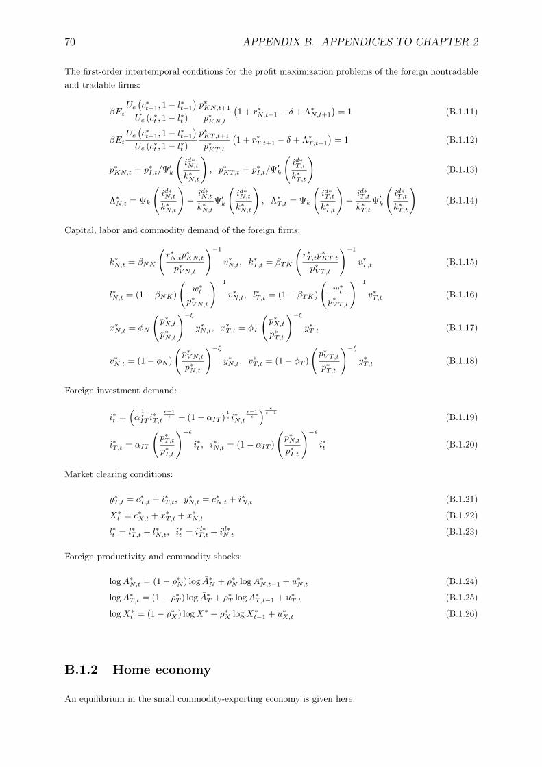
70 APPENDIX B. APPENDICES TO CHAPTER 2
The first-order intertemporal conditions for the profit maximization problems of the foreign nontradable
and tradable firms:
βEtUc(c∗t+1, 1− l∗t+1
)Uc (c∗t , 1− l∗t )
p∗KN,t+1
p∗KN,t
(1 + r∗N,t+1 − δ + Λ∗N,t+1
)= 1 (B.1.11)
βEtUc(c∗t+1, 1− l∗t+1
)Uc (c∗t , 1− l∗t )
p∗KT,t+1
p∗KT,t
(1 + r∗T,t+1 − δ + Λ∗T,t+1
)= 1 (B.1.12)
p∗KN,t = p∗I,t/Ψ′k
(id∗N,tk∗N,t
), p∗KT,t = p∗I,t/Ψ
′k
(id∗T,tk∗T,t
)(B.1.13)
Λ∗N,t = Ψk
(id∗N,tk∗N,t
)−id∗N,tk∗N,t
Ψ′k
(id∗N,tk∗N,t
), Λ∗T,t = Ψk
(id∗T,tk∗T,t
)−id∗T,tk∗T,t
Ψ′k
(id∗T,tk∗T,t
)(B.1.14)
Capital, labor and commodity demand of the foreign firms:
k∗N,t = βNK
(r∗N,tp
∗KN,t
p∗V N,t
)−1v∗N,t, k∗T,t = βTK
(r∗T,tp
∗KT,t
p∗V T,t
)−1v∗T,t (B.1.15)
l∗N,t = (1− βNK)
(w∗tp∗V N,t
)−1v∗N,t, l∗T,t = (1− βTK)
(w∗tp∗V T,t
)−1v∗T,t (B.1.16)
x∗N,t = φN
(p∗X,tp∗N,t
)−ξy∗N,t, x∗T,t = φT
(p∗X,tp∗T,t
)−ξy∗T,t (B.1.17)
v∗N,t = (1− φN )
(p∗V N,tp∗N,t
)−ξy∗N,t, v∗T,t = (1− φT )
(p∗V T,tp∗T,t
)−ξy∗T,t (B.1.18)
Foreign investment demand:
i∗t =(α
1ε
IT i∗T,t
ε−1ε + (1− αIT )
1ε i∗N,t
ε−1ε
) εε−1
(B.1.19)
i∗T,t = αIT
(p∗T,tp∗I,t
)−εi∗t , i∗N,t = (1− αIT )
(p∗N,tp∗I,t
)−εi∗t (B.1.20)
Market clearing conditions:
y∗T,t = c∗T,t + i∗T,t, y∗N,t = c∗N,t + i∗N,t (B.1.21)
X∗t = c∗X,t + x∗T,t + x∗N,t (B.1.22)
l∗t = l∗T,t + l∗N,t, i∗t = id∗T,t + id∗N,t (B.1.23)
Foreign productivity and commodity shocks:
logA∗N,t = (1− ρ∗N ) log A∗N + ρ∗N logA∗N,t−1 + u∗N,t (B.1.24)
logA∗T,t = (1− ρ∗T ) log A∗T + ρ∗T logA∗T,t−1 + u∗T,t (B.1.25)
logX∗t = (1− ρ∗X) log X∗ + ρ∗X logX∗t−1 + u∗X,t (B.1.26)
B.1.2 Home economy
An equilibrium in the small commodity-exporting economy is given here.

B.1. THE MODEL WITH COMPLETE MARKETS 71
The first-order conditions for the home representative household’s problem are:
qt,t+1Uc (ct, 1− lt) = βUc (ct+1, 1− lt+1) (B.1.27)
wtUc (ct, 1− lt) = Ul (ct, 1− lt) (B.1.28)
Home demand on aggregate consumption good and its components:
ct =(α
1ε
CT cε−1ε
T,t + α1ε
CNcε−1ε
N,t + (1− αCT − αCN )1ε c
ε−1ε
X,t
) εε−1
(B.1.29)
cT,t = αCT p−εT,tct, cN,t = αCNp
−εN,tct, cX,t = (1− αCT − αCN )p−εX,tct (B.1.30)
cT,t =(α
1θ
CHcθ−1θ
H,t + (1− αCH)1θ c
θ−1θ
F,t
) θθ−1
(B.1.31)
cH,t = αCH
(pH,tpT,t
)−θcT,t, cF,t = (1− αCH)
(pF,tpT,t
)−θcT,t (B.1.32)
Value added and output of the home tradable and nontradable firms and real GDP in terms of the home
consumption good:
vN,t = AN,tkβNKN,t l
1−βNKN,t , vT,t = AT,tk
βTKT,t l
1−βTKT,t (B.1.33)
yN,t =
((1− φN )
1ξ v
ξ−1ξ
N,t + φ1ξ
Nxξ−1ξ
N,t
) ξξ−1
(B.1.34)
yT,t =
((1− φT )
1ξ v
ξ−1ξ
T,t + φ1ξ
Txξ−1ξ
T,t
) ξξ−1
(B.1.35)
yt = pH,tyT,t + pN,tyN,t + pX,t(Xt − xT,t − xN,t) (B.1.36)
Capital in the home economy:
kN,t+1 = (1− δ)kN,t + kN,tΨk
(idN,tkN,t
)(B.1.37)
kT,t+1 = (1− δ)kT,t + kT,tΨk
(idT,tkT,t
)(B.1.38)
The first-order intertemporal conditions for the profit maximization problems of the home nontradable
and tradable firms:
βEtUc (ct+1, 1− lt+1)
Uc (ct, 1− lt)pKN,t+1
pKN,t(1 + rN,t+1 − δ + ΛN,t+1) = 1 (B.1.39)
βEtUc (ct+1, 1− lt+1)
Uc (ct, 1− lt)pKT,t+1
pKT,t(1 + rT,t+1 − δ + ΛT,t+1) = 1 (B.1.40)
pKN,t = pI,t/Ψ′k
(idN,tkN,t
), pKT,t = pI,t/Ψ
′k
(idT,tkT,t
)(B.1.41)
ΛN,t = Ψk
(idN,tkN,t
)−idN,tkN,t
Ψ′k
(idN,tkN,t
), ΛT,t = Ψk
(idT,tkT,t
)−idT,tkT,t
Ψ′k
(idT,tkT,t
)(B.1.42)

72 APPENDIX B. APPENDICES TO CHAPTER 2
Capital, labor and commodity demand of the home firms:
kN,t = βNK
(rN,tpKN,tpV N,t
)−1vN,t, kT,t = βTK
(rT,tpKT,tpV T,t
)−1vT,t (B.1.43)
lN,t = (1− βNK)
(wt
pV N,t
)−1vN,t, lT,t = (1− βTK)
(wtpV T,t
)−1vT,t (B.1.44)
xN,t = φN
(pX,tpN,t
)−ξyN,t, xT,t = φT
(pX,tpH,t
)−ξyT,t (B.1.45)
vN,t = (1− φN )
(pV N,tpN,t
)−ξyN,t, vT,t = (1− φT )
(pV T,tpH,t
)−ξyT,t (B.1.46)
Home investment demand:
it =(α
1ε
IT iε−1ε
T,t + (1− αIT )1ε i
ε−1ε
N,t
) εε−1
(B.1.47)
iT,t = αIT
(pIT,tpI,t
)−εit, iN,t = (1− αIT )
(pN,tpI,t
)−εit (B.1.48)
iT,t =(α
1θ
IHiθ−1θ
H,t + (1− αIH)1θ i
θ−1θ
F,t
) θθ−1
(B.1.49)
iH,t = αIH
(pH,tpIT,t
)−θiT,t, iF,t = (1− αIH)
(pF,tpIT,t
)−θiT,t (B.1.50)
Market clearing conditions:
yT,t = cH,t + c∗H,t + iH,t + i∗H,t, yN,t = cN,t + iN,t (B.1.51)
lt = lT,t + lN,t, it = idT,t + idN,t (B.1.52)
Home productivity and commodity shocks:
logAN,t = (1− ρN ) log AN + ρN logAN,t−1 + uN,t (B.1.53)
logAT,t = (1− ρT ) log AT + ρT logAT,t−1 + uT,t (B.1.54)
logXt = (1− ρX) log X + ρX logXt−1 + uX,t (B.1.55)
B.1.3 International trade and prices
Foreign demand on home tradable good:
c∗H,t = (1− αH)
(pH,tpF,t
)−θc∗T,t (B.1.56)
i∗H,t = (1− αH)
(pH,tpF,t
)−θi∗T,t (B.1.57)
Trade balance of the home economy:
tbt = pH,t(c∗H,t + i∗H,t) + pX,t(Xt − cX,t − xT,t − xN,t)− pF,t(cF,t + iF,t) (B.1.58)
The law of one price:
pX,t = etp∗X,t, pF,t = etp
∗T,t, qt,t+1 =
etet+1
q∗t,t+1 (B.1.59)

B.2. THE MODEL OF FINANCIAL AUTARKY 73
The law of one price for Arrow-Debreu securities and the first-order intertemporal conditions for the
households’ problems imply that:
etUc (ct, 1− lt) = ϑ0Uc (c∗t , 1− l∗t ) (B.1.60)
where ϑ0 is constant for all times and contingencies.
B.2 The model of financial autarky
The equilibrium conditions are the same as in the model with complete markets except of the law of one
price for financial assets and the intertemporal first-order conditions for the representative household’s
problems which are not satisfied in this model.
The only additional equilibrium condition is a balanced trade equation:
tbt = pH,t(c∗H,t + i∗H,t) + pX,t(Xt − cX,t − xT,t − xN,t)− pF,t(cF,t + iF,t) = 0 (B.2.1)
This model implies state and time-varying wedge ϑt between the cross-country marginal rate of substi-
tution of consumption and the real exchange rate:
etUc (ct, 1− lt) = ϑtUc (c∗t , 1− l∗t ) (B.2.2)
B.3 The model with portfolio adjustment costs
The equilibrium conditions are the same as in the model with complete markets except of the intertem-
poral first-order condition for the household problem, which in this model is given by the following
equation:
qt,t+1 = βUc (ct+1, 1− lt+1)
Uc (ct, 1− lt)1 + pN,t+1Ψ′a (Et+1qt+1,t+2at+2 − at+1)
1 + pN,tΨ′a (Etqt,t+1at+1 − at)(B.3.1)
This condition implies imperfect international risk sharing:
etUc (ct, 1− lt) = ϑtUc (c∗t , 1− l∗t ) (B.3.2)
where
ϑt =ϑ0
1 + pN,tΨ′a (Etqt,t+1at+1 − at)(B.3.3)
Given the presence of portfolio adjustment costs, market clearing condition for the home nontradable
goods is:
yN,t = cN,t + iN,t + Ψa (Etqt,t+1at+1 − at) (B.3.4)

74 APPENDIX B. APPENDICES TO CHAPTER 2
B.4 Figures
Figure B.1: Real commodity price, real exchange rate and consumption differential:Canada and Norway
-.20
-.15
-.10
-.05
.00
.05
.10
-.3
-.2
-.1
.0
.1
.2
.3
75 80 85 90 95 00 05 10
Relative Consumption: CAN vs. USAREER: CAN
-.1
.0
.1
.2
-.16
-.12
-.08
-.04
.00
.04
75 80 85 90 95 00 05 10
Relative Consumption: NOR vs. EUREER: NOR
-1.2
-0.8
-0.4
0.0
0.4
-.3
-.2
-.1
.0
.1
.2
.3
75 80 85 90 95 00 05 10
Real Commodity Price: CANREER: CAN
-2.0
-1.5
-1.0
-0.5
0.0
0.5
-.16
-.12
-.08
-.04
.00
.04
75 80 85 90 95 00 05 10
Real Commodity Price: NORREER: NOR
-1.2
-0.8
-0.4
0.0
0.4
-.04
.00
.04
.08
75 80 85 90 95 00 05 10
Real Commodity Price: CANTrade Balance (% of GDP): CAN
-1.5
-1.0
-0.5
0.0
0.5
-.1
.0
.1
.2
75 80 85 90 95 00 05 10
Real Commodity Price: NORTrade Balance (% of GDP): NOR

B.4. FIGURES 75
Figure B.2: Real commodity price, real exchange rate and consumption differential: Aus-tralia and New Zealand
-.08
-.04
.00
.04
.08
.12
-.2
.0
.2
.4
75 80 85 90 95 00 05 10
Relative Consumption: AUS vs. USAREER: AUS
-.3
-.2
-.1
.0
.1
.2
-.2
-.1
.0
.1
.2
.3
75 80 85 90 95 00 05 10
Relative Consumption: NZ vs. AUSREER: NZ
-1.2
-0.8
-0.4
0.0
0.4
-.4
-.2
.0
.2
.4
75 80 85 90 95 00 05 10
Real Commodity Price: AUSREER: AUS
-.8
-.4
.0
-.2
-.1
.0
.1
.2
.3
75 80 85 90 95 00 05 10
Real Commodity Price: NZREER: NZ
-1.2
-0.8
-0.4
0.0
0.4
-.04
-.02
.00
.02
75 80 85 90 95 00 05 10
Real Commodity Price: AUSTrade Balance (% of GDP): AUS
-.8
-.4
.0
-.15
-.10
-.05
.00
.05
75 80 85 90 95 00 05 10
Real Commodity Price: NZTrade Balance (% of GDP): NZ

76 APPENDIX B. APPENDICES TO CHAPTER 2
Figure B.3: International price levels in selected commodity exporting countries (% ofUSA)
0.4
0.6
0.8
1.0
1.2
1.4
1.6
1.8
0.4
0.6
0.8
1.0
1.2
1.4
1.6
1.8
1970 1975 1980 1985 1990 1995 2000 2005
AUS CAN NOR NZ

B.4. FIGURES 77
Figure B.4: Impulse responses to the foreign commodity shock
0 20 40−10
−5
0
% d
ev. f
rom
SS
X*
0 20 40−5
0
5
10
pX*
0 20 40−2
−1
0
% d
ev. f
rom
SS
y*
0 20 40−0.5
0
0.5y
0 20 40−3
−2
−1
0
% d
ev. f
rom
SS
yT*
0 20 40−4
−2
0
2
yT
0 20 40−1.5
−1
−0.5
0
% d
ev. f
rom
SS
yN*
0 20 40−2
−1
0
1
yN
CM
FA
PAC
ICM
Note. CM is the model with complete markets, FA is the model of financial autarky, PAC is themodel with portfolio adjustment costs, ICM is the model with incomplete markets.X∗ is a foreign commodity endowment, p∗X is a real commodity price, y (y∗) denotes real GDP in thehome (foreign) economy, yT (y∗T ) is an output of tradable goods in the home (foreign) economy and yN(y∗N ) denotes output of nontradable goods in the home (foreign) economy.

78 APPENDIX B. APPENDICES TO CHAPTER 2
Figure B.5: Impulse responses to the foreign commodity shock
0 20 40−1
−0.5
0
% d
ev. f
rom
SS
c*
0 20 40−1
−0.5
0
0.5c
0 20 40−1.5
−1
−0.5
0
% d
ev. f
rom
SS
cT*
0 20 40−2
−1
0
1
cT
0 20 40−1
−0.5
0
% d
ev. f
rom
SS
cN*
0 20 40−1
−0.5
0
0.5
cN
0 20 40−1
−0.5
0
0.5
% d
ev. f
rom
SS
l*
0 20 40−1
−0.5
0
0.5l
CM
FA
PAC
ICM
Note. CM is the model with complete markets, FA is the model of financial autarky, PAC is themodel with portfolio adjustment costs, ICM is the model with incomplete markets.c (c∗) denotes aggregate consumption in the home (foreign) economy, cT (c∗T ) is a consumption oftradable goods, cN (c∗N ) is a consumption of nontradable goods and l (l∗) denotes hours worked in thehome (foreign) economy.

B.4. FIGURES 79
Figure B.6: Impulse responses to the foreign commodity shock
0 20 40−4
−2
0
2
% d
ev. f
rom
SS
i*
0 20 40−5
0
5i
0 20 40−5
0
5
% d
ev. f
rom
SS
iT*
0 20 40−5
0
5
iT
0 20 40−4
−2
0
2
% d
ev. f
rom
SS
iN*
0 20 40−4
−2
0
2
iN
0 20 40−10
−5
0
5
% d
ev. f
rom
SS
cH*
0 20 40−10
−5
0
5
iH*
CM
FA
PAC
ICM
Note. CM is the model with complete markets, FA is the model of financial autarky, PAC is themodel with portfolio adjustment costs, ICM is the model with incomplete markets.i (i∗) denotes aggregate investment in the home (foreign) economy, iT (i∗T ) is investment expenditure ontradable goods, iN (i∗N ) is investment expenditure on nontradable goods, c∗H and i∗H denote respectivelyforeign consumer and investment demands on the home tradable goods.
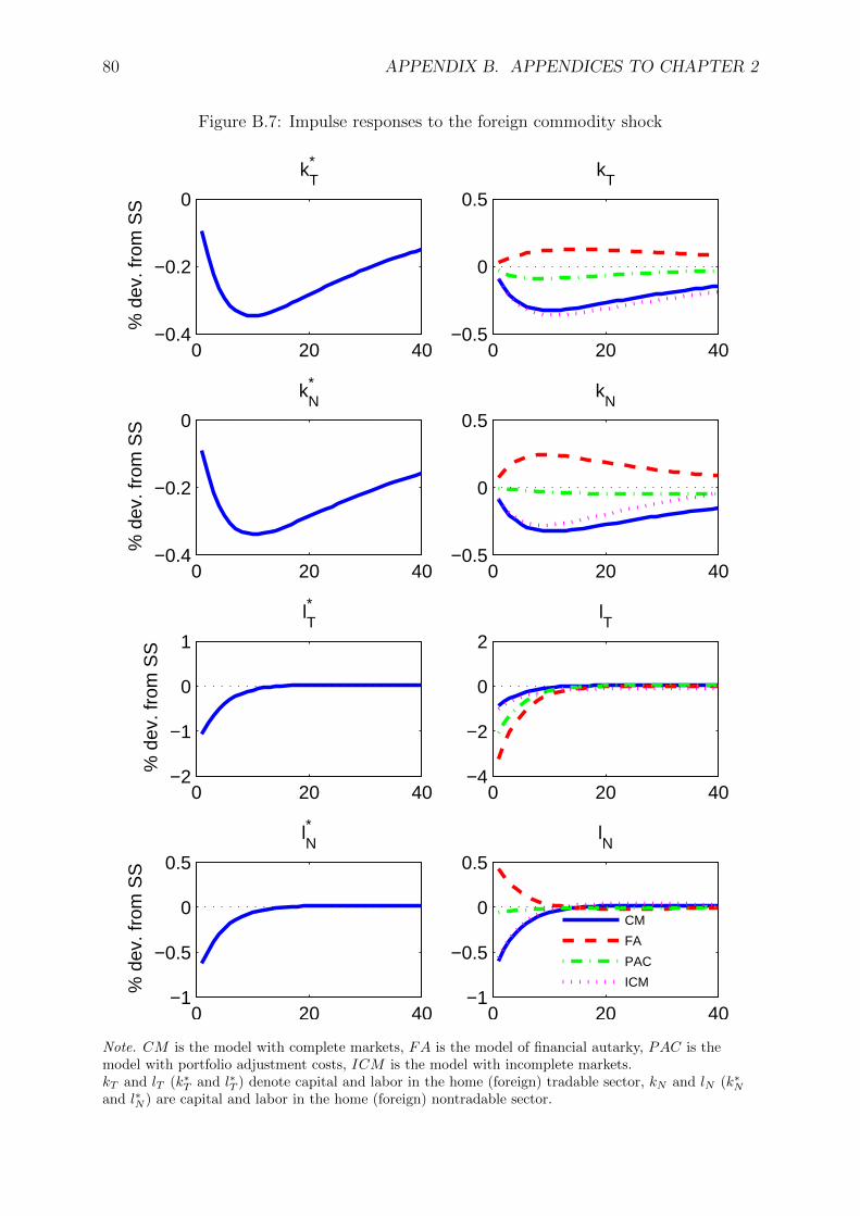
80 APPENDIX B. APPENDICES TO CHAPTER 2
Figure B.7: Impulse responses to the foreign commodity shock
0 20 40−0.4
−0.2
0
% d
ev. f
rom
SS
kT*
0 20 40−0.5
0
0.5
kT
0 20 40−0.4
−0.2
0
% d
ev. f
rom
SS
kN*
0 20 40−0.5
0
0.5
kN
0 20 40−2
−1
0
1
% d
ev. f
rom
SS
lT*
0 20 40−4
−2
0
2
lT
0 20 40−1
−0.5
0
0.5
% d
ev. f
rom
SS
lN*
0 20 40−1
−0.5
0
0.5
lN
CM
FA
PAC
ICM
Note. CM is the model with complete markets, FA is the model of financial autarky, PAC is themodel with portfolio adjustment costs, ICM is the model with incomplete markets.kT and lT (k∗T and l∗T ) denote capital and labor in the home (foreign) tradable sector, kN and lN (k∗Nand l∗N ) are capital and labor in the home (foreign) nontradable sector.

B.4. FIGURES 81
Figure B.8: Impulse responses to the foreign commodity shock
0 20 40−1
0
1
2
% o
f GD
Ptb
0 20 40−4
−2
0
2
% d
ev. f
rom
SS
e
0 20 40−1
−0.5
0
0.5
% d
ev. f
rom
SS
pN* /p
T*
0 20 40−1
0
1
2
pN
/pT
0 20 40−2
0
2
4
% d
ev. f
rom
SS
pH
/pF
0 20 40−1
−0.5
0
0.5
pI
0 20 40−1.5
−1
−0.5
0
% d
ev. f
rom
SS
w*
0 20 40−2
−1
0
1w
CM
FA
PAC
ICM
Note. CM is the model with complete markets, FA is the model of financial autarky, PAC is themodel with portfolio adjustment costs, ICM is the model with incomplete markets.
tb denotes trade balance (as a share of GDP) in the home economy, e is a real exchange rate, pNpT (p∗Np∗T
) is
a relative price of the nontradable and tradable goods in the home (foreign) economy, pHpF is a relative
price of the home and foreign tradable goods, pI denotes real investment price, w (w∗) is a real wage inthe home (foreign) economy.

82 APPENDIX B. APPENDICES TO CHAPTER 2
Figure B.9: Impulse responses to the foreign productivity shock in nontradable sector
0 20 400
0.5
1
1.5
% d
ev. f
rom
SS
AN*
0 20 400
0.5
1
1.5
pX*
0 20 400
0.5
1
% d
ev. f
rom
SS
y*
0 20 40−0.05
0
0.05y
0 20 40−0.2
0
0.2
% o
f GD
P
tb
0 20 40−1.5
−1
−0.5
0
% d
ev. f
rom
SS
e
0 20 40−1.5
−1
−0.5
0
% d
ev. f
rom
SS
pN* /p
T*
0 20 40−0.2
0
0.2
pN
/pT
CMFAPACICM
Note. CM is the model with complete markets, FA is the model of financial autarky, PAC is themodel with portfolio adjustment costs, ICM is the model with incomplete markets.A∗N is a productivity in the foreign nontradable sector, p∗X is a real commodity price, y (y∗) denotes realGDP in the home (foreign) economy, tb denotes trade balance (as a share of GDP) in the home
economy, e is a real exchange rate, pNpT (p∗Np∗T
) is a relative price of the nontradable and tradable goods in
the home (foreign) economy.

B.4. FIGURES 83
Figure B.10: Impulse responses to the foreign productivity shock in tradable sector
0 20 400
1
2
3
% d
ev. f
rom
SS
AT*
0 20 400
0.5
1
pX*
0 20 400
0.5
1
% d
ev. f
rom
SS
y*
0 20 400
0.2
0.4y
0 20 40−0.05
0
0.05
% o
f GD
P
tb
0 20 40−0.5
0
0.5
% d
ev. f
rom
SS
e
0 20 40−1
0
1
2
% d
ev. f
rom
SS
pN* /p
T*
0 20 40−0.5
0
0.5
1
pN
/pT
CM
FA
PAC
ICM
Note. CM is the model with complete markets, FA is the model of financial autarky, PAC is themodel with portfolio adjustment costs, ICM is the model with incomplete markets.A∗T is a productivity in the foreign tradable sector, p∗X is a real commodity price, y (y∗) denotes realGDP in the home (foreign) economy, tb denotes trade balance (as a share of GDP) in the home
economy, e is a real exchange rate, pNpT (p∗Np∗T
) is a relative price of the nontradable and tradable goods in
the home (foreign) economy.

84 APPENDIX B. APPENDICES TO CHAPTER 2
B.5 Tables

B.5. TABLES 85
Table B.1: Business cycles statistics for some commodity-exporting countries
1970Q1-2008Q1 1985Q1-2008Q1Levels HP-filtered Levels HP-filtered
std(pX)Australia 29.72 8.82 22.64 8.83Canada 27.96 9.08 22.39 9.26Norway 39.41 14.16 34.42 15.48New Zealand 27.35 7.95 14.45 7.32
std(e)Australia 16.62 5.68 9.98 6.06Canada 13.69 3.52 11.31 3.47Norway 4.45 2.69 4.22 2.60New Zealand 9.65 5.90 10.75 6.47
corr(c− c∗, e)Australia -0.117 -0.345 -0.284 -0.309Canada -0.699 -0.040 -0.746 -0.310Norway -0.073 0.038 -0.181 0.232New Zealand -0.229 -0.264 -0.283 -0.522
corr(pX , i)Australia 0.252 0.289Canada 0.326 0.272Norway -0.209 -0.238New Zealand 0.310 0.418
corr(pX , e)Australia -0.865 -0.412 -0.786 -0.561Canada -0.681 -0.193 -0.617 -0.412Norway -0.478 -0.135 -0.525 -0.249New Zealand -0.175 -0.351 -0.578 -0.457
corr(pX , tb)Australia 0.091 0.132Canada 0.276 0.430Norway 0.670 0.785New Zealand 0.005 0.200
Note. All the variables except trade balance are in logarithms. pX is real world price index of exportedcommodities, y is GDP in terms of consumption good, i is investment, c− c∗ is consumption differentialwith main trade partner, e is effective real exchange rate and tb is trade balance in % of GDP.Data. OECD EO, EcoWin

86 APPENDIX B. APPENDICES TO CHAPTER 2
Table B.2: Calibration
Parameters Value
Preferences β 0.99γ 0.38σ 2
Aggregates ε 0.74θ 1.5aCT 0.23aCN 0.73aCH 0.68aIT 0.38aIH 0.31
Technology δ 0.025ξ 0.69bTK 0.34bNK 0.34φT 0.20φN 0.10A∗T 3.13A∗N 3.13X∗ 1.00AT 2.47AN 2.88X 1.41
Shocks ρX , ρ∗X 0.80
std(uX), std(u∗X) 4.60, 6.90ρT , ρ
∗T 0.80
std(uT ), std(u∗T ) 2.30, 2.30ρN , ρ
∗N 0.80
std(uN), std(u∗N) 1.15, 1.15
Adjustment costs ψ 0.6d -0.005

B.5. TABLES 87T
able
B.3
:B
reak
dow
nof
indust
ries
into
com
modit
y,tr
adab
lean
dnon
trad
able
sect
ors:
Can
ada,
2000
ISIC
Industry
Valueadded
Tra
detu
rnover
Netexport
MFP
code
(%of
GD
P)
(%of
Gro
ssou
tpu
t)(%
ofG
ross
outp
ut)
(%of
US
)Primary
commodityindustries
16.3
70.0
16.4
98
A,B
Agr
icu
ltu
re,
hu
nti
ng,
fore
stry
and
fish
ing
2.2
29.8
7.4
65C
Min
ing
and
qu
arry
ing
6.1
75.8
31.6
102
D20
Wood
and
pro
du
cts
ofw
ood
an
dco
rk1.
364
.949
.110
0D
21-2
2P
ulp
,p
aper
,p
rinti
ng
and
pub
lish
ing
2.5
65.0
26.4
114
D23
Cok
e,re
fin
edp
etro
leu
mp
rod
uct
san
dnu
clea
rfu
el0.
231
.08.
767
D24
Ch
emic
als
and
chem
ical
pro
du
cts
1.4
116.
1-2
3.2
97D
25R
ub
ber
and
pla
stic
sp
rod
uct
s0.
999
.814
.473
D26
Oth
ern
on-m
etal
lic
min
eral
pro
du
cts
0.5
64.7
-11.
610
6D
27B
asic
met
als
1.2
91.7
10.4
123
Tra
dable
good
industries
28.6
81.5
-2.5
79
D15
-16
Food
pro
du
cts,
bev
erag
esan
dto
bac
co2.
143
.83.
410
2D
17-2
0T
exti
les,
texti
lep
rod
uct
s,le
ath
eran
dfo
otw
ear
0.8
141.
4-4
1.1
80D
28F
abri
cate
dm
etal
pro
du
cts
1.4
83.3
-4.2
69D
29M
ach
iner
yan
deq
uip
men
t,n
.e.c
1.3
206.
0-6
2.1
99D
30O
ffice
,ac
counti
ng
and
com
pu
tin
gm
ach
iner
y0.
138
7.3
-126
.978
D31
Ele
ctri
cal
mac
hin
ery
and
app
aratu
s,n
.e.c
.0.
723
3.0
-72.
883
D32
Rad
io,
tele
vis
ion
and
com
mu
nic
atio
neq
uip
men
t0.
516
5.9
21.0
83D
33M
edic
al,
pre
cisi
onan
dop
tica
lin
stru
men
ts0.
323
0.9
-87.
183
D34
Mot
orve
hic
les,
trail
ers
an
dse
mi-
trai
lers
2.5
152.
39.
212
8D
35O
ther
tran
spor
teq
uip
men
t0.
914
4.0
18.9
128
D36
-37
Fu
rnit
ure
,m
anu
fact
uri
ng
n.e
.c.,
recy
clin
g0.
711
4.6
18.0
73I6
0-63
Tra
nsp
ort
4.0
28.2
21.2
88J
Fin
ance
and
insu
rance
6.2
16.5
-6.1
66K
72C
omp
ute
ran
dre
late
dact
ivit
ies
1.3
27.1
16.0
66K
74O
ther
bu
sin
ess
acti
vit
ies
5.8
23.8
-3.2
59Nontradable
good
industries
55.1
5.9
2.8
92
EE
lect
rici
ty,
gas
and
wat
ersu
pp
ly2.
613
.19.
560
FC
onst
ruct
ion
5.0
0.0
0.0
135
GW
hol
esal
ean
dre
tail
trad
e,re
pai
rs13
.39.
86.
091
HH
otel
san
dre
stau
rants
2.3
21.7
10.4
93I6
4P
ost
and
tele
com
mu
nic
atio
ns
2.5
11.7
0.6
68K
70-7
1,73
Rea
les
tate
,re
nti
ng,
rese
arch
an
dd
evel
opm
ent
11.9
1.5
0.0
66L
Pu
bli
cad
min
.an
dd
efen
se,
com
p.
soci
alse
curi
ty7.
21.
11.
099
ME
du
cati
on4.
71.
51.
211
8N
Hea
lth
and
soci
alw
ork
2.4
1.4
-1.3
118
OO
ther
com
mu
nit
y,so
cial
and
per
son
alse
rvic
es3.
113
.34.
164
P,Q
Pri
vate
hou
seh
old
sw
ith
emp
loye
dp
erso
ns
0.2
0.0
0.0
118

88 APPENDIX B. APPENDICES TO CHAPTER 2
Table B.4: Steady state equilibrium
Variable Foreign Home
OutputGDP y 6.46 6.23production of tradables yT 1.69 1.19production of nontradables yN 4.57 4.37production of commodity X 1.00 1.41
Consumptiontotal c 5.14 4.99
tradables cT 1.18 1.16home tradables cH 0.66foreign tradables cF 0.53
nontradables cN 3.75 3.60commodity cX 0.21 0.24
Investmenttotal i 1.32 1.30
tradables iH 0.50 0.53home tradables iF 0.11foreign tradables iH 0.43
nontradables iF 0.82 0.77Capital
total k 52.93 51.82in tradable sector kT 13.06 11.08in nontradable sector kN 39.87 40.74
Employmenttotal l 0.30 0.29
in tradable sector lT 0.07 0.06in nontradable sector lN 0.23 0.23
Commodity inputin tradable sector xT 0.34 0.31in nontradable sector xN 0.46 0.52
Exporthome tradables 0.43
for consumption c∗H 0.22for investment i∗H 0.20
commodity 0.34Import
foreign tradables 0.95
Price of tradables pT 1.00 0.99of home tradables pH 1.12of foreign tradables pF 0.78
Price of nontradables pN 1.00 1.02Price of capital goods pK 1.00 0.96Commodity price pX 1.00 0.78Wage w 11.99 11.53Capital return r 0.04 0.04Real exchange rate e 0.78

B.5. TABLES 89T
able
B.5
:B
usi
nes
scy
cles
stat
isti
cs
Sta
tist
ics
Dat
aM
odel
Can
ada
For
eign
Hom
e
1985
Q1-
2008
Q1
Com
ple
teF
inan
cial
Adju
stm
ent
Mar
kets
Auta
rky
Cos
ts
Sta
nda
rdD
ev.
GD
P1.
782.
24(.
06)
1.55
(.03
)1.
71(.
04)
1.62
(.04
)O
utp
ut
oftr
adab
les
4.19
13.
31(.
08)
3.47
(.08
)4.
40(.
12)
3.92
(.09
)O
utp
ut
ofnon
trad
able
s1.
691
1.86
(.05
)1.
91(.
05)
1.54
(.04
)1.
56(.
04)
Con
sum
pti
on0.
911.
32(.
04)
1.31
(.03
)0.
92(.
02)
0.99
(.03
)In
vest
men
t4.
125.
75(.
15)
5.70
(.14
)6.
09(.
16)
4.13
(.11
)E
mplo
ym
ent
1.12
0.95
(.03
)0.
86(.
02)
0.56
(.01
)0.
68(.
02)
Tra
de
bal
ance
(%of
GD
P)
0.91
1.90
(.05
)0.
00(.
)0.
90(.
02)
Rea
lco
mm
odit
ypri
ce9.
269.
51(.
25)
Rea
lex
chan
gera
te3.
471.
39(.
04)
5.56
(.15
)3.
18(.
08)
Cro
ss-c
orre
lati
ons
Bet
wee
nre
alco
mm
odit
ypri
cean
dG
DP
0.58
-0.7
1(.
02)
-0.0
6(.
03)
0.17
(.03
)0.
06(.
03)
Outp
ut
oftr
adab
les
-0.0
81-0
.64
(.02
)-0
.61
(.02
)-0
.77
(.02
)-0
.71
(.02
)O
utp
ut
ofnon
trad
able
s0.
021
-0.5
6(.
02)
-0.6
2(.
02)
0.03
(.04
)-0
.35
(.03
)In
vest
men
t0.
27-0
.65
(.02
)-0
.72
(.02
)0.
50(.
03)
-0.0
8(.
04)
Rea
lex
chan
gera
te-0
.41
-0.0
7(.
04)
-0.8
1(.
01)
-0.7
6(.
02)
Tra
de
bal
ance
0.43
0.84
(.01
)0.
00(.
)0.
84(.
01)
Bet
wee
nre
alex
chan
gera
tean
dR
elat
ive
consu
mpti
on-0
.31
1.00
(.)
-0.4
5(.
03)
0.04
(.03
)B
etw
een
fore
ign
and
hom
eG
DP
0.62
0.12
(.04
)-0
.07
(.03
)0.
01(.
03)
Con
sum
pti
on0.
630.
66(.
02)
0.15
(.04
)0.
50(.
02)
Inve
stm
ent
0.49
0.70
(.02
)-0
.23
(.03
)0.
26(.
03)
Em
plo
ym
ent
0.70
0.88
(.01
)0.
74(.
02)
0.85
(.01
)
aan
nu
ald
ata

90 APPENDIX B. APPENDICES TO CHAPTER 2
Tab
leB
.6:B
usin
esscy
clesstatistics:
foreigncom
modity
shock
s
Statistics
Model
Foreign
Hom
e
Com
plete
Fin
ancial
Adju
stmen
tM
arketsA
utark
yC
osts
Stan
dar dD
ev.G
DP
1.86(.05)
0.14(.)
0.26(.01)
0.08(.)
Trad
ebalan
ce(%
ofG
DP
)1.61
(.04)0.00
(.)0.77
(.02)R
ealcom
modity
price
9.39(.26)
Real
exch
ange
rate0.07
(.)4.38
(.12)2.26
(.06)C
ross-correlations
Betw
eenreal
comm
odity
price
and
GD
P-0.85
(.01)0.98
(.)0.99
(.)R
ealex
chan
gerate
0.99(.)
-1.00(.)
-1.00(.)
Trad
ebalan
ce1.00
(.)0.00
(.)1.00
(.)B
etween
realex
chan
gerate
and
Relative
consu
mption
1.00(.)
-0.98(.)
-0.98(.)

B.5. TABLES 91
Tab
leB
.7:
Busi
nes
scy
cles
stat
isti
cs:
fore
ign
pro
duct
ivit
ysh
ock
sin
trad
able
sect
or
Sta
tist
ics
Model
For
eign
Hom
e
Com
ple
teF
inan
cial
Adju
stm
ent
Mar
kets
Auta
rky
Cos
ts
Sta
nda
rdD
ev.
GD
P0.
66(.
02)
0.24
(.01
)0.
23(.
01)
0.24
(.01
)T
rade
bal
ance
(%of
GD
P)
0.06
(.)
0.00
(.)
0.03
(.)
Rea
lco
mm
odit
ypri
ce0.
93(.
03)
Rea
lex
chan
gera
te0.
25(.
01)
0.10
(.)
0.17
(.)
Cro
ss-c
orre
lati
ons
Bet
wee
nre
alco
mm
odit
ypri
cean
dG
DP
1.00
(.)
1.00
(.)
1.00
(.)
Rea
lex
chan
gera
te-1
.00
(.)
-0.9
9(.
)-1
.00
(.)
Tra
de
bal
ance
-1.0
0(.
)0.
00(.
)-1
.00
(.)
Bet
wee
nre
alex
chan
gera
tean
dR
elat
ive
consu
mpti
on1.
00(.
)1.
00(.
)1.
00(.
)

92 APPENDIX B. APPENDICES TO CHAPTER 2
Tab
leB
.8:B
usin
esscy
clesstatistics:
foreignpro
ductiv
itysh
ock
sin
non
tradab
lesector
Statistics
Model
Foreign
Hom
e
Com
plete
Fin
ancial
Adju
stmen
tM
arketsA
utark
yC
osts
Stan
dar dD
ev.G
DP
1.07(.03)
0.00(.)
0.05(.)
0.03(.)
Trad
ebalan
ce(%
ofG
DP
)0.18
(.)0.00
(.)0.09
(.)R
ealcom
modity
price
1.44(.04)
Real
exch
ange
rate0.94
(.03)1.43
(.04)1.20
(.03)C
ross-correlations
Betw
eenreal
comm
odity
price
and
GD
P0.59
(.02)0.99
(.)0.99
(.)R
ealex
chan
gerate
-1.00(.)
-1.00(.)
-1.00(.)
Trad
ebalan
ce0.99
(.)0.00
(.)0.99
(.)B
etween
realex
chan
gerate
and
Relative
consu
mption
1.00(.)
1.00(.)
1.00(.)

B.5. TABLES 93
Tab
leB
.9:
Sen
siti
vit
yan
alysi
s
Sta
tist
ics
Xθ
std(u∗ X
)
11.
413
0.74
1.5
154.
66.
99.
2
Sta
nda
rdD
ev.
GD
P1.
561.
621.
851.
551.
621.
961.
621.
621.
62O
utp
ut
oftr
adab
les
3.97
3.92
3.70
2.95
3.92
9.31
3.31
3.92
4.61
Outp
ut
ofnon
trad
able
s1.
601.
561.
531.
571.
561.
521.
501.
561.
63C
onsu
mpti
on1.
060.
990.
891.
010.
990.
940.
890.
991.
12In
vest
men
t4.
094.
134.
674.
024.
134.
704.
114.
134.
16E
mplo
ym
ent
0.80
0.68
0.47
0.64
0.68
1.16
0.52
0.68
0.86
Tra
de
bal
ance
(%of
GD
P)
0.82
0.90
0.98
0.85
0.90
1.17
0.71
0.90
1.13
Rea
lco
mm
odit
ypri
ce9.
519.
519.
519.
559.
519.
556.
479.
5112
.61
Rea
lex
chan
gera
te2.
743.
184.
243.
393.
183.
082.
713.
183.
76C
ross
-cor
rela
tion
sB
etw
een
real
com
modit
ypri
cean
dG
DP
-0.1
60.
060.
37-0
.04
0.06
0.33
0.05
0.06
0.08
Inve
stm
ent
-0.2
8-0
.08
0.28
-0.1
7-0
.08
0.15
-0.0
3-0
.08
-0.1
2R
eal
exch
ange
rate
-0.7
1-0
.76
-0.8
1-0
.72
-0.7
6-0
.74
-0.6
4-0
.76
-0.8
4T
rade
bal
ance
0.83
0.84
0.86
0.83
0.84
0.82
0.72
0.84
0.90
Bet
wee
nre
alex
chan
gera
tean
dR
elat
ive
consu
mpti
on0.
230.
04-0
.25
0.16
0.04
-0.1
90.
270.
04-0
.17
Bet
wee
nfo
reig
nan
dhom
eG
DP
0.19
0.01
-0.2
40.
130.
01-0
.24
0.04
0.01
-0.0
2C
onsu
mpti
on0.
560.
500.
320.
520.
500.
380.
300.
500.
63In
vest
men
t0.
400.
26-0
.04
0.34
0.26
0.06
0.25
0.26
0.27
Em
plo
ym
ent
0.88
0.85
0.60
0.86
0.85
0.68
0.72
0.85
0.90

94 APPENDIX B. APPENDICES TO CHAPTER 2

Chapter 3
International risk sharing and
optimal monetary policy in a small
commodity-exporting economy
3.1 Introduction
It is commonly acknowledged that high volatility in commodity prices has important
effects on global economic activity. However, less attention has been paid to analyze the
effect of this volatility on small commodity-exporting economies, where primary resources
constitute an essential source of export revenues. In these countries, commodity-price
movements have enormous impacts on a wide range of macroeconomic variables, including
balance of payments, exchange rates, output and public finance. As a result, these effects
pose serious problems for the conduct of macroeconomic policy in such economies.
In particular, it has been stressed in the literature (Chen and Rogoff, 2003; Cashin
et al., 2004) that real exchange rates in commodity-exporting economies exhibit two salient
regularities: (i) they are very volatile and (ii) they are negatively correlated with world
commodity prices. Hence, price hikes of basic commodities are usually associated with a
real exchange rate appreciation and, conversely, price drops are linked to a real deprecia-
tion. This empirical regularity is known in economic literature as the commodity currency
effect, a phenomenon which is illustrated in Figure C.1 for four developed commodity-
exporting countries: Canada, Norway, Australia and New Zealand.1
Moreover, commodity currency effect poses a problem for the conduct of monetary
policy in such economies since fluctuations of the real exchange rate induced by commodity
price changes render impossible the joint achievement of stable prices and stable nominal
1Standard deviations of the real commodity price index, real effective exchange rate and their cross-correlations (for HP-filtered series) for the period 1985q1-2008q1 are respectively: 9.3, 3.5 and -0.41 forCanada, 15.5, 2.6 and -0.25 for Norway, 8.8, 6.1 and -0.56 for Australia, 7.3, 6.5 and -0.46 for NewZealand.
95

96 CHAPTER 3. RISK SHARING AND OPTIMAL MONETARY POLICY
exchange rate.2 Accordingly, there is a trade-off between these two basic goals of monetary
policy and the choice of the nominal exchange rate regime (flexible vs. fixed) has nontrivial
welfare implications. Given that inflation is very costly in an environment with sticky
consumer prices, a common suggestion in the open-economy literature is to allow the
nominal exchange rate to float freely in these economies, absorbing in this way the volatile
terms-of-trade shocks (e.g., this type of policy recommendation has been made for Canada
and Russia in Dib (2008) and Sosunov and Zamulin (2007), respectively).
In line with this prescription, many central banks in commodity-exporting economies
have adopted a goal of low and stable inflation. For instance, all developed commodity-
exporting economies (Australia, Canada, Norway, New Zealand and Iceland) and many
fast-growing emerging economies (Chile, Brazil, South Africa) pursue an explicit core
inflation target while the nominal exchange rate is allowed to float freely in order to
act as a shock absorber. There are, however, exceptions to this rule like many Gulf
oil producers which peg their currencies to US dollar or Russia and Kazakhstan which
manage the nominal exchange rate fluctuations using interventions (partially sterilized)
in the foreign exchange markets. The monetary policy authorities in these countries
often claim that the main rationale for these operations is to reduce volatility of the real
exchange rate and to alleviate the danger of a Dutch disease.3 Nonetheless, it is often
the case that this policy succeeds in smoothing real exchange rate fluctuations, but at the
cost of a high (often two-digit) and unstable inflation.
In view of these different monetary policy experiences, the goal of this chapter is to
analyze under which conditions the adoption of a fixed nominal exchange rate might not be
such a bad policy per se for small commodity-exporting economies. In particular, I argue
that the volatility of the real exchange rate and, as a result, the welfare costs of the fixed
regime depend crucially on the extent of risk sharing between the commodity-exporting
economy and the rest of the world. One can think of two alternative setups. On the one
hand, under the assumption of complete and frictionless asset markets, such an economy
may be perfectly insured against foreign commodity shocks, rendering no significant effects
on the real exchange rate so that welfare losses from the fixed nominal exchange rate
become negligible. On the other hand, the existence of frictions in international assets
trade renders too costly a complete insurance against foreign commodity shocks. In such
a case, the windfall income gains from commodity exports are spent partially at home
2Note, that the rate of change of the real exchange rate is given (in logs) by ∆qt = ∆et + π∗t − πt,where ∆et is the rate of change of the nominal exchange rate, and πt and π∗t denote domestic andforeign inflation respectively. So, under an assumption of stable foreign prices, fluctuations in the realexchange rate have to be accommodated either by changes in the nominal exchange rate, or by domesticinflation/deflation.
3Dutch disease is an economic concept that explains the relationship between the increase in exportrevenues from basic commodities and a decline in the non-commodity tradable sector (mainly manufac-turing). The underlying mechanism is the following. An increase in export of primary commodities willappreciate real exchange rate, making non-commodity exports more expensive. As a result, the manu-facturing sector becomes less competitive and its output declines (see Corden, 1984, for more details).
3.1. INTRODUCTION 97
and this puts pressure on the real exchange rate so that welfare costs of the fixed nominal
exchange rate regime might be large.
Specifically, to analyze quantitatively the welfare effects of the world commodity price
shocks under alternative regimes of the monetary policy, I propose a multi-sector New
Keynesian model of small commodity-exporting economy which can be calibrated to es-
timate the welfare costs in each situation. This model features three production sectors:
primary commodity, non-commodity tradable and nontradable sectors. The world econ-
omy is modeled explicitly as in Gali and Monacelli (2005) and Charnavoki (2009). There-
fore in contrast to the existing literature for small commodity-exporting economies (for
example Dib, 2008; Sosunov and Zamulin, 2007), the world commodity price fluctuations
in this model (as well as the other world prices and demands) are not treated as shocks
per se, but are rather considered to be endogenously determined outcomes. This allows us
to control directly the extent of international risk sharing. The representative households
trade a complete set of financial assets, but portfolio pay-offs bear transaction costs. By
varying the degree of financial transaction costs, it is possible to cover a full spectrum of
model economies ranging from perfect international risk sharing to financial autarky.4
The formulation of the proposed model takes into consideration several stylized fea-
tures of primary commodities which have been highlighted in this strand of the literature.
First, primary commodities are assumed to be a homogeneous good in the sense that many
firms supply goods with similar characteristics and qualities that are traded in organized
exchanges or have a reference price (Rauch, 1999). By contrast, tradable and nontradable
goods are produced in varieties, differentiated both across and within countries.
Secondly, while prices of primary commodities are very flexible (Bils and Klenow, 2004;
Gopinath and Rigobon, 2008), there is significant heterogeneity in the frequencies of price
changes for manufactured goods and services.5 Therefore, nominal prices of primary
4Our model is related to the existing theoretical literature studying international risk-sharing, namelyBackus-Smith and real exchange rate volatility puzzles, in the context of two-country models. A numberof papers explain these puzzles using models with incomplete asset markets. So, for example, Benignoand Thoenissen (2007) study a model with nontradable and tradable goods sectors. To obtain a negativecorrelation between relative consumption and the real exchange rate they assume that productivity shocksto the tradable sector are more persistent and more volatile than those in the nontradable one. Corsetti,Dedola, and Leduc (2008) argue that the implied elasticity of substitution between tradable goods islow since nontradable goods are used in the distribution of tradables. This feature allows them to solveBackus-Smith and real exchange rate volatility puzzles in the model with single traded asset. However,an assumption of incomplete asset markets in stochastic framework of small open economy model resultsin non-stationary equilibrium dynamics. To induce stationarity standard models usually assume non-separable preferences or some form of frictions in assets trade (Schmitt-Grohe and Uribe, 2003). Yet,these additional elements might resolve the aforementioned puzzles in the framework with completemarkets too. For example, Bodenstein (2008) develops a two-country model with complete asset marketsand limited enforcement for international financial contracts that provides a possible explanation of thesetwo puzzles. At the same time, Verdelhan (2010) uses habit preferences to explain excess volatility of thereal exchange rate.
5Bils and Klenow (2004) report that in US 54.3% prices of raw goods are changed every monthcomparing to 20.5% prices of processed goods and 20.7% prices of services. Gopinath and Rigobon (2008)use US export/import data and estimate monthly frequencies of price changes 83%(73%) and 30%(27%)

98 CHAPTER 3. RISK SHARING AND OPTIMAL MONETARY POLICY
commodities in the model are asummed to be flexible, whereas price rigidities in the non-
commodity tradable and nontradable sectors are modelled using conventional Calvo-Yun
contracts. It is also assumed that a fraction of prices of exported non-commodity goods
is quoted in foreign currency (local currency pricing) while the rest is quoted in domestic
currency (producer-currency pricing).
Lastly, output and labor productivity of industries producing primary commodities
(agriculture, fishing, mining, etc.) are significantly more volatile than in manufacturing,
services or construction (see global sector-specific shocks in Koren and Tenreyro, 2007).
This can be observed in Table C.1 which presents, for a sample of OECD countries, the
standard deviations of labor productivity in commodity-production sectors (agriculture,
fishing, mining, etc.), as well as in tradable (manufacturing) and nontradable (services,
utilities and construction) sectors. Labor productivity in the commodity sector is on
average twice and four times more volatile than in the tradable and nontradable sectors,
respectively. Together with an inelastic demand on commodities, this fact could explain
an excess volatility of the commodity prices.
While monetary policy in the rest of the world is supposed to be conducted in an
optimal way, four monetary policy regimes are considered for small commodity-exporting
economy: credible peg of the nominal exchange rate, targeting core consumer inflation,6
targeting domestic non-commodity output inflation and optimal policy with commitment.
For the welfare computations, we use a second-order approximations to the welfare and
policy functions around the deterministic steady state following the approach advocated
by Schmitt-Grohe and Uribe (2004).7
The welfare comparisons of the alternative monetary policy regimes are related to the
existing distortions. In this respect, I abstract from the monopolistic distortion that in-
duces an inefficient level of output by introducing offsetting subsidy, and instead focus on
other two sources of inefficiency to trade off in our model of small commodity-exporting
economy. First, in response to asymmetric disturbances, nominal rigidities create an inef-
ficient dispersion of prices within tradable and nontradable sectors as well as an inefficient
path of the domestic and international (terms of trade, real exchange rates) relative prices.
Second, financial frictions generate a wedge between the marginal utility differential in the
home and world economies and real exchange rate, resulting in demand disequilibria (in
terminology of Corsetti, Dedola, and Leduc, 2010). Further, in the case of local currency
pricing, there are deviations from the law of one price, resulting in inefficiency in the
supply of tradable goods due to price dispersion in domestic and foreign markets. Finally,
for import(export) goods traded on organized exchanges and having reference price respectively comparingto 7%(7%) for differentiated import(export) goods.
6Core CPI does not include primary commodity component.7A standard welfare analysis of the model of open economy using second-order approximation to the
welfare function but linear approximation to policy function may provide spurious results (see Kim andKim, 2003).

3.1. INTRODUCTION 99
as stressed by many authors (see in particular Corsetti and Pesenti (2001) and Benigno
and Benigno (2003)), there is strategic element in open-economy monetary policy since
monetary authorities may affect terms of trade in a beneficial for home economy way.
The main findings are the following. In accordance with the existing literature, the
welfare comparisons show that a fixed nominal exchange rate regime is, in general, domi-
nated by a flexible regime. However, the welfare costs of the fixed regime vary significantly
with the extent of international risk sharing and with the size of home commodity sector.
As discussed earlier, under assumption of complete and frictionless asset markets, welfare
losses from the nominal peg are small. Alternatively, if the commodity sector is too small,
the home economy cannot generate significant windfall income from commodity exports
so that, even under financial autarky, the fixed regime is not very costly. In sum, it is
only in the case of a large commodity sector and imperfect financial markets that a fixed
regime implies high welfare costs.
This result underscores the practical importance for small commodity-exporting economies
of adopting some kind of cross-country risk-sharing mechanisms, which would allow them
to stabilize their real exchange rates while reducing the welfare costs of keeping the nom-
inal exchange rate pegged. In practice this may be implemented by either hedging in
commodity futures markets,8 or creating some form of the stabilization fund,9 or even
participating in a full-fledged fiscal union (see Frankel, 2010, for a good review).
Another relevant implication of our analysis is related to the welfare properties of the
flexible nominal exchange rate regimes. We show that core consumer inflation targeting
and non-commodity domestic inflation targeting turn out to be not optimal in general,
though their welfare costs are small comparing to fixed regime. Further, the welfare
ranking of these two regimes may depend on the currency in which tradable goods are
priced (producer currency pricing vs. local currency pricing). Under producer currency
pricing domestic inflation targeting is preferable to core consumer inflation targeting while
the opposite holds under local currency pricing.
This rest of the chapter is organized as follows. Section 2 presents the main features
of the model for a small commodity-exporting economy. Section 3 discusses calibration
of the parameters and shocks. Section 4 reports and discusses simulations results: de-
terministic steady-state, impulse responses to unitary innovations in foreign commodity
shocks and the main business cycle statistics. Section 5 measures and discusses the welfare
implications of the alternative monetary policy regimes. Section 6 concludes.
8Believing oil prices would eventually fall, Mexico hedged in 2008 almost all of next’s year oil exportsat prices ranging from $70 to $100 at a cost of about $1.5bn through derivatives contracts. Accordingto Financial Times, this move paid off handsomely, resulting in over $5bn in profit when the price of oilcollapsed in 2009.
9At present time, many resource-abundant countries and regions accumulate a fraction of their com-modity revenues in sovereign wealth funds. We can recall here, for instance, Government Pension Fundof Norway, Reserve Fund of Russia, Alaska Permanent Fund, Permanent Wyoming Mineral Trust Fundor Alberta Heritage Fund.

100 CHAPTER 3. RISK SHARING AND OPTIMAL MONETARY POLICY
3.2 Model
This section starts by presenting a model of the world economy in its more general format.
Next, specific assumptions about productivities, commodity endowments and monetary
policies are made to reduce this model to the small commodity-exporting economy/the
world economy case.
Notation is as follows. Variables with an i subscript refer to economy i, one among
the continuum of economies making up the world economy. Variables without an i-index
denote a small commodity-exporting economy being modelled. Finally, variables with a
star superscript correspond to the world economy as a whole (typical foreign economy).
3.2.1 General description of the model
The world economy is modeled as a continuum of small open economies represented by a
unit interval, as in Gali and Monacelli (2005). Since each economy is of measure zero, its
domestic policy decisions do not have any impact on the rest of the world. We abstract
here from the monetary frictions and interpret this model as cashless limiting case (see
Woodford, 2003). Assets markets therefore are complete.
A typical small economy produces three types of goods: differentiated tradable good,
differentiated nontradable good and homogeneous tradable primary commodity. Tradable
goods and commodity can be used for consumption either in the domestic economy or
abroad, whereas nontradable goods are consumed only in the home country. Firms pro-
ducing tradable and nontradable goods, as well as commodity endowments, are owned by
domestic households.
The world economy is affected by productivity shocks in tradable and nontradable
sectors as well as by shocks to commodity endowments.
3.2.2 Households
A typical small economy i is inhabited by a representative household who owns domestic
tradable and nontradable firms and supplies labor to them. This household maximizes
expected life-time utility:
maxCt(i),LN,t(i),LT,t(i),Dt+1(i,st+1)
E0
∞∑t=0
βt
(C1−σt (i)
1− σ− χ−νN (i)
L1+νN,t (i)
1 + ν− χ−νT (i)
L1+νT,t (i)
1 + ν
)(3.2.1)

3.2. MODEL 101
subject to a sequence of budget constraints expressed in terms of domestic currency:
Pt(i)Ct(i) +
∫Qt,t+1(i, st+1)Dt+1(i, st+1)dst+1 + PN,t(i)Ψ
(Dt(i)
Pt(i)
)≤
≤ Dt(i) +WN,t(i)LN,t(i) +WT,t(i)LT,t(i) + Πt(i)− Tt(i)(3.2.2)
where Ct(i) is a consumption, Lk,t(i) denotes hours worked in sector k ∈ N, T, Dt+1(i, st+1)
are the holdings of state-contingent claims, priced at Qt,t+1(i, st+1), paying off one unit
of domestic currency in the realized state of the world st+1, Pt(i) denotes a consumption
price index, Wk,t(i) is nominal wage in sector k, Πt(i) denotes profits from the domestic
firms and commodity endowment and Tt(i) are lump-sum taxes/transfers.10
Note, that labor is imperfectly mobile between domestic tradable and nontradable
firms. We assign the weights χT (i) and χN(i) in such a way, that wages in both sectors
would be equalized in a deterministic steady-state equilibrium.
Given the assumption of the complete assets markets, the currency composition of
financial assets can be ignored. So, to simplify notation, only the nominal pay-offs de-
nominated in domestic currency are posted here. Prices of the state-contingent claims
paying off in currency i and j are linked in the following way:
Qt,t+1(i) = Qt,t+1(j)Et(i, j)Et+1(i, j)
(3.2.3)
where Et(i, j) is bilateral nominal exchange rate (price of currency j in terms of currency
i).
The convex function Ψ(s) reflects the financial intermediation costs and satisfies the
following assumptions: Ψ(s) ≥ 0, Ψ(0) = Ψ′(0) = 0 and Ψ′′(0) = ψ > 0. In particular,
I assume quadratic costs: Ψ(s) = ψ s2
2. These transaction costs allow us to control risk
sharing between domestic and foreign economies. In the limit, when ψ → ∞, economy
i becomes an financial autarky. Another extreme case: ψ = 0, corresponds to perfect
international risk sharing.11 Without loss of generality, we assume also that these financial
intermediation costs are paid in terms of nontradable goods.
The composite consumption good Ct is a CES basket of the tradable CT,t, nontradable
CN,t goods and commodity CX,t:
Ct(i) =(α
1εTC
ε−1ε
T,t (i) + α1εNC
ε−1ε
N,t (i) + (1− αT − αN)1εC
ε−1ε
X,t (i)) εε−1
(3.2.4)
10Note that money does not appear in the budget constraint. We assume here that central bank candirectly control nominal short-run interest rate paid on risk-free assets. Hence, money plays here onlythe role of unit of account.
11The model of small open economy with incomplete markets and null transaction costs (ψ = 0) ischaracterized by nonstationary equilibrium dynamics (in contrast to complete markets case). Non-zerofinancial intermediation costs may be used to make price of the debt sensitive to its size and thereforeto avoid nonstationarity issue. See Schmitt-Grohe and Uribe (2003) for alternative ways to deal withnonstationarity in the model of small open economy.

102 CHAPTER 3. RISK SHARING AND OPTIMAL MONETARY POLICY
where ε denotes an elasticity of substitution between tradable goods, nontradable goods
and commodity (gross complementarity is assumed: ε < 1) and αT and αN reflect the
weights of tradable and nontradable goods in composite index.
The index of tradable goods CT,t is in turn a CES basket of the home CH,t and foreign
CF,t tradable goods:
CT,t(i) =(α
1θHC
θ−1θ
H,t (i) + (1− αH)1θC
θ−1θ
F,t (i)) θθ−1
(3.2.5)
where θ is the elasticity of substitution between home and foreign tradable goods (with
ε < θ) and αH reflects a home bias in consumption of tradable goods.
Nontradable, home tradable and foreign tradable indexes, CN,t, CH,t and CF,t respec-
tively, are aggregates of varieties:
CN,t(i) =
(∫ 1
0
CηN−1
ηNN,t (i, n)dn
) ηNηN−1
, CH,t(i) =
(∫ 1
0
CηT−1
ηTT,t (i, i, h)dh
) ηTηT−1
CF,t(i) =
(∫ 1
0,j 6=i
∫ 1
0
CηT−1
ηTT,t (i, j, h)dhdj
) ηTηT−1
(3.2.6)
where CN,t(i, n) is country i consumption of nontradable variety n, CT,t(i, j, h) is country
i consumption of tradable variety h produced in country j, ηN and ηT are the elasticities
of substitution among varieties in nontradable and tradable sectors respectively.
Households allocate their consumption by solving expenditure minimization problem
(taking prices of goods as given).
3.2.3 Firms and commodity endowments
The markets for tradable and nontradable goods in the model are characterized by mo-
nopolistic competition. It is assumed that the only variable factor of production is labor.
Typical firms producing nontradable and tradable goods have the following production
functions:
YN,t(i, n) = AN,t(i)LN,t(i, n), YT,t(i, h) = AT,t(i)LT,t(i, h) (3.2.7)
where AN,t(i) and AT,t(i) are productivity levels, respectively, in nontradable and tradable
sectors in the country i, LN,t and LT,t are labor inputs.
Staggered pricing a-la Calvo-Yun in nontradable and tradable sectors are assumed
(Calvo, 1983). In particular, a fraction 0 < ωN < 1 of nontradable goods prices remains
unchanged each period, whereas new prices are optimally chosen for the other fraction
1− ωN of nontradable goods.
Since the firms are owned by domestic households, the present value of future profits

3.2. MODEL 103
is discounted according to the household’s intertemporal marginal rate of substitution in
consumption:
Ft,τ (i) = βτ−t(Cτ (i)
Ct(i)
)−σPt(i)
Pτ (i)(3.2.8)
A firm that changes its price in period t chooses PN,t(i) to maximize the expected dis-
counted stream of profits:
maxPN,t(i)
Et
∞∑τ=t
ωτ−tN Ft,τ (i)(PN,t(i)− (1− sN)
WN,τ (i)
AN,τ (i)
)(PN,t(i)PN,τ (i)
)−ηNYN,τ (i) (3.2.9)
where YN,τ (i) = CN,τ (i) + 12ψ(Dτ (i)Pτ (i)
)2is aggregate demand on nontradable goods.
To induce an efficient level of output government subsidizes the firms with rate sN
and finances this subsidy by lump-sum taxes on domestic households.
The price index of nontradable goods PN,t(i) is then determined as:
PN,t(i) =(ωNP
1−ηNN,t−1(i) + (1− ωN)P1−ηN
N,t (i)) 1
1−ηN (3.2.10)
Pricing decisions of the tradable firms are more complicated, given that these firms can
set their prices either in home or in foreign currency. It is assumed here that a share γ of
all domestic firms in that sector use producer currency pricing (PCP). These firms solve
the following problem:
maxPPT,t(i)
Et
∞∑τ=t
ωτ−tT Ft,τ (i)(PPT,t(i)− (1− sT )
WT,τ (i)
AT,τ (i)
)×
×
((PPT,t(i)PH,τ (i)
)−ηTCH,τ (i) +
∫ 1
0,j 6=i
(PPT,t(i)
Eτ (i, j)PF,τ (j)
)−ηTCF,τ (j)dj
) (3.2.11)
where sT is an offsetting subsidy to tradable firms.
The remaining fraction 1 − γ of domestic tradable firms set their prices using local
currency pricing (LCP):
maxPLT,t(i,j)j
Et
∞∑τ=t
ωτ−tT Ft,τ (i)
(PLT,t(i, i)− (1− sT )
Wτ (i)
AT,τ (i)
)(PLT,t(i, i)PH,τ (i)
)−ηTCH,τ (i)+
+
∫ 1
0,j 6=i
(Eτ (i, j)PLT,t(i, j)− (1− sT )
Wτ (i)
AT,τ (i)
)(PLT,t(i, j)PF,τ (j)
)−ηTCF,τ (j)dj
(3.2.12)
where PLT,t(i, j) are the optimal prices chosen by tradable firms of country i using LCP

104 CHAPTER 3. RISK SHARING AND OPTIMAL MONETARY POLICY
for their export to country j.
The indices of home and foreign tradable goods are then determined as:
P 1−ηTH,t (i) = ωTP
1−ηTH,t−1(i) + (1− ωT )γPP1−ηT
T,t (i) + (1− ωT )(1− γ)PL1−ηTT,t (i, i)
P 1−ηTF,t (i) = ωTP
1−ηTF,t−1(i) + (1− ωT )γ
∫ 1
0,j 6=i
(Et(i, j)PPT,t(j)
)1−ηT dj++ (1− ωT )(1− γ)
∫ 1
0,j 6=iPL1−ηTT,t (j, i)dj
(3.2.13)
where PPT,t(i) and PLT,t(i, j) are optimal prices chosen by tradable firms of country i in
period t using, respectively, producer currency and local currency pricing.
Output in commodity sector is exogenously determined and does not incur costs.
Therefore, the profits of this sector are just the commodity endowment Xt times its price
PX,t:
ΠX,t(i) = PX,t(i)Xt(i) (3.2.14)
3.2.4 Governments
The budget constraint of the government in country i is given by the following equation:
Tt(i) = sNWN,t(i)LN,t(i) + sTWT,t(i)LT,t(i) (3.2.15)
where Tt(i) are lump-sum taxes levied on domestic households to finance offsetting sub-
sidies skWk,t(i)Lk,t(i) to firms in sector k ∈ T,N.
3.2.5 Market clearing conditions
All goods, factors and assets markets clear at any time and any contingency.
Market clearing for the tradable, nontradable goods and commodity requires:
YN,t(i, n) = CN,t(i, n) +
(PN,t(i, n)
PN,t(i)
)−ηN ψ2
(Dt(i)
Pt(i)
)2
,∀i, n, t
YT,t(i, h) =
∫ 1
0
CT,t(j, i, h)dj, ∀i, h, t,∫ 1
0
Xt(i)di =
∫ 1
0
CX,t(i)di,∀t(3.2.16)
The aggregate supply of the labor has to be equal to the aggregate demand of labor in
both nontradable and tradable sectors:
LN,t(i) =
∫ 1
0
LN,t(i, n)dn,∀i, t, LT,t(i) =
∫ 1
0
LT,t(i, h)dh,∀i, t (3.2.17)
Finally, the total supply of assets in the world economy is zero at any time and any
3.2. MODEL 105
contingency:∫ 1
0
Dt(i, st)Et(j, i)di = 0,∀j, t, st (3.2.18)
3.2.6 Productivity and commodity shocks
So far we have presented a very general model of the world economy. To specify this model
for the small commodity-exporting economy/the world economy case we need to introduce
several assumptions about productivities, commodity endowments and monetary policy.
First of all, among the continuum of small open economies we choose one economy
of measure zero labeled as home economy. All other (foreign) economies are completely
symmetric: they are driven by the same productivities in nontradable and tradable sectors,
A∗N,t and A∗T,t, and commodity endowments, X∗t . Besides, they share a common currency.
As a result, a typical foreign economy represents the world economy as whole.
The home economy is assumed to be commodity abundant:
AN = A∗N , AT = A∗T , X > X∗ (3.2.19)
where AT (A∗T ), AN(A∗N), and X(X∗) denote steady-state productivity of tradable and
nontradable firms and commodity endowments in home (foreign) country respectively.
The commodity and productivity shocks in home and world economies are assumed
to follow independent AR(1) processes:
logAk,t = (1− ρk)Ak + ρk logAk,t−1 + uk,t, k ∈ N, T
logXt = (1− ρX)X + ρX logXt−1 + uX,t
logA∗k,t = (1− ρk)A∗k + ρk logA∗k,t−1 + u∗k,t, k ∈ N, T
logX∗t = (1− ρX)X∗ + ρX logX∗t−1 + u∗X,t
(3.2.20)
where the disturbance terms uk,t are normally distributed.
3.2.7 Monetary policy
To close the model we need to specify monetary policy at both the home and the world
economies. We assume that all (symmetric) foreign economies share common currency
and that monetary policy in this currency union is conducted in an optimal way with
commitment. Since the home economy is of measure zero, its policy decisions have no
effect on the world economy. The world economy is closed and, given that wages and
commodity prices are flexible, targeting the weighted index of tradable and nontradable
prices render optimal policy in this economy (see Chapter 6, Section 4.3 in Woodford,
2003; Aoki, 2001). Under assumption that frequencies of price changes and elasticities

106 CHAPTER 3. RISK SHARING AND OPTIMAL MONETARY POLICY
in tradable and nontradable sectors are equal, ωN = ωT and ηN = ηT , this weighted
index coincides with the core consumer price index, i.e. consumer price index without
commodity component.
I consider four alternative monetary policy regimes for small commodity-exporting
economy. The first is credible fixed nominal exchange rate regime (FER):
∆et = log
(EtEt−1
)= 0,∀t (3.2.21)
where Et is the nominal exchange rate of the home currency.
The second regime is strict core CPI inflation targeting (CIT):
πB,t = log
(PB,tPB,t−1
)= 0,∀t (3.2.22)
where PB,t =(
αNαN+αT
P 1−εN,t + αT
αN+αTP 1−εT,t
) 11−ε
is core consumer price index.
The third regime is strict non-commodity domestic output inflation targeting (DIT):
πD,t = log
(PD,tPD,t−1
)= 0,∀t (3.2.23)
where πD,t =Y nD,tYD,t
is the GDP deflator in tradable and nontradable sectors with Y nD,t and
YD,t denoting, respectively, nominal and real GDP in these sectors.
Lastly, to characterize an optimal monetary policy with commitment (OP) for home
economy we need to formulate an infinite-horizon Lagrangian problem where central bank
maximizes conditional expected social welfare function:
Wt0 = Et0
∞∑t=t0
βt
(C1−σt
1− σ− χ−νN
L1+νN,t
1 + ν− χ−νT
L1+νT,t
1 + ν
)(3.2.24)
subject to the full set of equilibrium conditions for home and foreign economies for all
t ≥ t0 (implementability constraints) and precommitment constraints for forward-looking
variables at t = t0.12 Note, that optimal policy is conducted in non-cooperative way.
Hence, monetary authority, having monopolistic power over domestic terms of trade, may
affect them in a beneficial way for the home economy (see in particular Corsetti and
Pesenti, 2001; Benigno and Benigno, 2003).
Appendix C.1 summarizes equilibrium conditions for the previous model of small
commodity-exporting economy/the world economy. Below, basic simulation results and
welfare evaluations under the four above-mentioned monetary policy regimes are provided
for a calibrated version of the model. Yet, before moving to the results, a brief discussion
12We consider here optimal policy from the timeless perspective, as e.g. in Woodford (2010) or Levin,Onatski, Williams, and Williams (2006).

3.3. CALIBRATION 107
of the model calibration strategy is in order.
3.3 Calibration
This section presents a calibration of the parameters and stochastic shocks for the pro-
posed model of a small commodity-exporting economy. The model is calibrated to quar-
terly data. Most parameters are standard and their values are taken from the literature.
The benchmark calibration is summarized in Table C.2.
We set the quarterly discount factor β equal to 0.99, which implies an annual steady-
state real interest rate of about 4%. The inverse of the intertemporal elasticity of substi-
tution, σ, is fixed at 2 as in most of the literature.13 The parameter ν plays dual role in
our model: on the one hand, its inverse determines the Frisch elasticity of labor supply
and, on the other, the elasticity of substitution of labor supply across tradable and non-
tradable firms. The value of the Frish elasticity is ambiguous, as stressed by Christiano,
Eichenbaum, and Evans (1997). In most of the microeconomic studies its estimate is very
small, often close to 0. By contrast, the real business cycles literature typically work with
labor supply elasticities of much higher magnitude, sometimes in excess of 5. Given this
wide the range, following Christiano et al. (1997), I use a benchmark value for ν, equal
to 1, which also corresponds to an estimate of cross-sectoral elasticity of substitution of
labor given by Horvath (2000) and Kim and Kim (2006).
The elasticity of substitution between tradables, nontradables and commodity, ε, is
set to 0.74 as in Mendoza (1991). There is some controversy about the value of trade
elasticity θ (see for example Ruhl (2004) for a good review). The elasticities considered in
the international real business cycles literature range from 0.5 to 2.0.14 I use value 1.5 as
in Backus et al. (1992). The elasticities of substitution between varieties in tradable and
nontradable sectors, ηT and ηN , are set to 11, what corresponds to price markups equal
to 10%. Parameters ωN and ωT are set equal to 0.75, a value consistent with an average
period of one year between price adjustments (as in Gali and Monacelli, 2005).
The consumption weights of tradable and nontradable goods, αT and αN , are set to
0.4 and 0.5 respectively, what corresponds roughly to non-energy goods and services in
the consumer price index for Canada. The home weight in consumption of tradable goods,
αH , is equal to 0.5 (according to input-output data for Canada).
The steady-state productivity levels in tradable and nontradable sectors are assumed
to be the same for home and foreign economies: AN = A∗N = AT = A∗T = 1. Commodity
endowment in the world economy, X∗, is set at 1 too. At the same time, three alternative
specifications for the home commodity sector are assumed. The first case, X = 1, corre-
sponds to ex-ante symmetric home economy. In this case there are no international trade
13See for example Backus et al. (1992)14The trade literature works with much higher elasticities in range from 10 to 15.

108 CHAPTER 3. RISK SHARING AND OPTIMAL MONETARY POLICY
in primary commodities in deterministic steady state. The second alternative, X = 4,
correspond to the chosen benchmark parametrization of a small commodity-exporting
economy. Finally, a model with large home commodity sector: X = 10 is considered.
To study the effect of financial frictions and international risk sharing, three variants
of the model are reported: (i) frictionless asset markets, ψ = 0; (ii) an intermediate
(benchmark) case with ψ = 1, and (iii) financial autarky with ψ → ∞. I also consider
two alternative pricing regime for home and foreign tradable firms: producer currency
pricing, γ = 1, and local currency pricing, γ = 0.
Finally, regarding the parameterization of the exogenous stochastic processes, the
persistence parameter, ρk, is set equal to 0.8 for all productivity and commodity shocks.
At the same time, volatilities of nontradable, tradable and commodity shocks are set to
0.01, 0.02 and 0.04 respectively (both for home and foreign economies). This corresponds
roughly to ratio for OECD countries (see Table C.1). Productivity and commodity shocks
are assumed to be uncorrelated across countries and sectors.
3.4 Simulation results
3.4.1 Deterministic steady-state equilibrium
It is convenient to start the discussion of the simulation results with a brief look at the
deterministic steady-state equilibrium. Given the cross-country asymmetry of the model,
this equilibrium allows us to identify long-run structural differences between the home
and world economies. It is assumed that, in steady state, both economies have balanced
trade and zero inflation.15 As a result, the corresponding equilibrium depends neither on
financial transaction costs ψ, nor on monetary policy regime nor on currency of pricing
for tradable goods γ.
A steady-state solution of the model is presented in Table C.3 under the three alter-
native assumptions about the steady-state home commodity endowment X. First, we
consider a symmetric case, X = 1, where home economy is identical to typical foreign
economy. Then we introduce two variants of the commodity-abundant home economy:
X = 4 and X = 10.
As expected, deterministic steady-state allocations and prices in home and foreign
economies coincide in a symmetric case. There is no international trade in commodity,
whereas home export and import are driven by intra-industry trade in (non-commodity)
tradable goods. Besides, the steady-state real exchange rate (i.e., the inverse of the
international price level) is equal to one.
15An optimal steady state exists in which the inflation rate is zero in our model with optimal monetarypolicy. We checked it by conjecturing that the solution involves zero inflation, and then determining thataugmented matrix of the system of N equations for N − 1 Lagrange multipliers has rank equal to N − 1.

3.4. SIMULATION RESULTS 109
In contrast, the model with commodity-abundant home economy generates important
asymmetries in the steady state. First, higher commodity endowment makes the home
economy wealthier than the foreign one. Households in the home economy enjoy higher
welfare, consume more nontradable, tradable and commodity goods (both in aggregate
terms and separately in each type of good), and also work less.
Second, international trade flows fit well with a law of comparative advantages: the
home country exports primary commodity whereas its imports of foreign tradable goods
exceed the exports of home tradables. Notice that this steady-state trade pattern captures
an important source of business cycle fluctuations for the small commodity-exporting
economy, since world commodity price changes may induce significant windfall incomes
(or losses) from commodity export.
Third, higher demand in home economy pushes up wages and prices of nontradable and
home tradable goods. At the same time, relative domestic prices of foreign tradable goods
and commodity fall. As a result, home consumption of foreign tradable goods increases,
whereas foreign consumption of home tradable goods falls. However, income and substi-
tution effects work in opposite direction for home demand on home tradable goods. In the
case of X = 4, the income effect dominates in steady state, so that home consumption of
its own tradables increases relative to the symmetric variant of the model. Conversely, the
substitution effect dominates in the case of large commodity sector, X = 10. Neverthe-
less, total demand (home and foreign) on home tradable goods unambiguously decreases.
Thus, output and labor in the home economy shifts from tradable to nontradable sector,
reproducing the main feature of the so-called Dutch disease.
Lastly, high relative prices of home nontradable and tradable goods result in a higher
international price level for the home economy relative to the foreign one (i.e, the steady-
state real exchange rate is now lower than 1).
3.4.2 Impulse responses
In this section, I illustrate the dynamic effects of the foreign commodity shocks on a
number of home macroeconomic variables. I focus here on the benchmark model with
intermediate financial transaction costs, ψ = 1, and average size of the home commodity
sector, X = 4.16 Figures C.2-C.7 display impulse responses to negative unitary innovation
in the foreign commodity endowment under the four monetary policy regimes.
A decrease in the foreign commodity endowment results in higher world real commod-
ity price. Besides, the size of the price increase exceeds the size of initial commodity shock,
since the demand for commodity is inelastic (elasticity of substitution between commod-
ity and non-commodity goods ε in our model is less than 1. Both foreign output and
consumption fall due to the immediate decrease in commodity supply and to the induced
16The model is solved in Dynare package for MATLAB. The first-order necessary conditions for optimalpolicy are computed using Andrew T. Levin’s code (Levin et al., 2006).

110 CHAPTER 3. RISK SHARING AND OPTIMAL MONETARY POLICY
reduction in the demand on nontradable and tradable goods. Since the foreign central
bank targets non-commodity consumer price inflation, core inflation does not change. At
the same time headline inflation rises following the rise in the price of its commodity
component.
Given that home economy is a net exporter of commodity in the deterministic steady
state, the rise of the world commodity price leads to increase in home trade balance.
Non-zero financial transaction costs hinder international risk sharing between home and
foreign households, so that windfall income from commodity exports is partly spent inside
of home economy. As a result, the real exchange rate appreciates whereas demand shifts
from commodity and home tradable goods to foreign tradable and home nontradable
goods, and labor switches from home tradable to nontradable firms.
Since the prices of tradable and nontradable goods are sticky in the short run, mone-
tary policy can manipulate real exchange rate (and therefore home and foreign demands)
to some extent. Under the producer currency pricing (PCP) regime, the nominal exchange
rate changes imply a full pass-through to import prices and therefore play a expenditure-
switching role. A central bank that targets core consumer inflation allows the nominal
exchange rate to float freely, absorbing the change in the real exchange rate. Domestic
non-commodity output inflation targeting and optimal policy have similar effects.17 By
contrast, in the case of fixed nominal exchange rate (and stable foreign consumer prices),
the real exchange rate may appreciate only slowly through consumer inflation in the home
economy. Hence, the real exchange rate appreciation is restrained but at the cost of higher
inflation. In other words, monetary policy is too loose in this case, and so consumption
and output in the home economy are higher than under flexible exchange rate regimes.
Under the local currency pricing (LCP) regime, the dynamic effects of an increase in
commodity prices on the home economy is similar. But, since in this case the nominal
exchange rate pass-through is zero, the expenditure-switching effect of the nominal ex-
change rate is hindered. Since an adjustment of the trade balance through changes in
relative prices is sluggish, the nominal exchange rate has to appreciate even more than
under PCP to comply with the international risk-sharing condition C.1.14. Given that
home tradable firms set their prices in local currency, the nominal appreciation results in
higher prices of home tradable goods for the domestic market than for the foreign market.
Thus, in contrast to PCP case, the law of one price for these goods fails. At the same
time, the relative price of nontradable vs. tradable consumption goods and the relative
price of home vs. foreign tradable consumption goods raise less strongly than in the PCP
case, due to the home currency pricing of the import goods.
17Since consumer price index includes imported consumer goods and under PCP their prices are cor-related with nominal exchange rate, core consumer inflation targeting places higher weight on stabilizingnominal exchange rate than other flexible regimes.

3.4. SIMULATION RESULTS 111
3.4.3 Business cycles statistics
This section is devoted to a brief discussion of the business-cycle properties of some
relevant macroeconomic variables under the four monetary policy regimes. I focus on
two business cycles moments: standard deviations and contemporary correlations with
the real foreign commodity price. These statistics are reported for models with different
values of the financial transaction costs parameter, ranging from perfect international risk
sharing, ψ = 0, to financial autarky, ψ → ∞.18 Table C.4 and Figure C.8 display these
business-cycle statistics generated by foreign commodity shocks only, whereas Table C.5
and Figure C.9 illustrate the results for all productivity and commodity shocks.
In the case of perfect international risk sharing, ψ = 0, the foreign commodity shocks
can be perfectly insured. Hence, volatility of the real exchange rate induced by these
shocks is close to zero and, as result, standard deviations of the core consumer inflation,
non-commodity domestic inflation and rate of change of the nominal exchange rate are
always small independently of monetary policy regime under consideration. The headline
consumer inflation volatility is determined exclusively by the growth rate of the price of
its commodity component.
Introduction of the financial frictions results in reduced volatility of the trade balance,
increased volatility of the real exchange rate and a negative correlation of the latter with
the real commodity price (commodity currency effect). Under a flexible nominal exchange
rate regime, obviously it translates into higher volatility of the nominal exchange rate.
By contrast, a currency peg implies higher volatility of inflation as well as its positive
correlation with the real commodity price. At the same time, the real exchange rate is
not surprisingly smoother under a fixed regime, reflecting short-run price stickiness. This
effect increases with rising financial costs.
Core consumer inflation targeting regime implies lower volatility of the nominal ex-
change rate relative to domestic inflation targeting and optimal monetary policy. This
result can be explained by the inclusion of import prices in the CPI, and a full pass-
through of the nominal exchange rate changes into those prices under PCP pricing.
Introduction of the other shocks does not alter the results significantly. The only
important difference is the non-zero volatility of the real exchange rate in the case of null
financial transaction costs, reflecting the impossibility of getting insurance against shocks
in the nontradable sector as well as the home bias in consumption of tradable goods.
Nevertheless, rising financial transaction costs increase real exchange rate volatility and
its negative correlation with real commodity price: as in the previous case this implies a
trade-off between stability of nominal exchange rate and inflation.
18For brevity, only the case of PCP pricing is presented here.

112 CHAPTER 3. RISK SHARING AND OPTIMAL MONETARY POLICY
3.5 Welfare analysis
This section reports the main results of the chapter. We evaluate welfare implications
of the fixed and flexible exchange rate regimes under alternative specifications of the
model of small commodity-exporting economy. This welfare analysis focusess on three
key parameters.
First, I compare welfare costs of the exchange rate regimes under three different as-
sumptions about the extent of international risk sharing (perfect international risk sharing,
ψ = 0, financial autarky, ψ → ∞, and an intermediate case, ψ = 1). Second, I analyze
the welfare implications of the different size of the home commodity sector. The first
case is the one where home and foreign economies are completely symmetric ex ante:
X = X∗ = 1. Then, I consider two variants of the commodity abundant small home
economy: X = 4 and X = 10. Finally, I report the results for two variants of the pricing
regime of the tradable firms: producer currency pricing, γ = 1, and local currency pricing,
γ = 0.
As before, the above-mentioned four monetary policy regimes are considered (credible
peg of the nominal exchange rate, targeting the core consumer inflation, targeting the
domestic output inflation and optimal policy with commitment). Results are reported
under two scenarios. The first one assumes that the only shock affecting the model
economy is a foreign commodity shock. Under the second scenario, the model is affected
by the full set of home and foreign productivity and commodity shocks.
To evaluate the welfare costs of the alternative monetary policy regimes, second-order
approximations of the welfare and policy functions are used (see Schmitt-Grohe and Uribe,
2004). Notice that a standard welfare analysis of the model of open economy using
second-order approximation to the welfare function but just a linear approximation to
policy function may provide spurious results. For example, Kim and Kim (2003) show
that in a simple two-agent economy, this standard method may yield higher welfare under
financial autarky than under perfect risk sharing. The problem is that some key second-
order terms of the equilibrium welfare function are omitted. Consequently, the resulting
criterion becomes inaccurate to order two.
3.5.1 Welfare metrics
I now describe the welfare metric used to evaluate exchange rate regimes. I adopt a
procedure proposed by Lucas (1991). More specifically, the unconditional welfare loss is
measured in terms of the fraction, ξ, of additional deterministic steady-state consumption
needed to equate the unconditional expected utility under uncertainty with the utility
obtained under the deterministic steady state:
U((1 + ξ)C, LN , LT ) = EU(Ct, LN,t, LT,t)
(3.5.1)

3.5. WELFARE ANALYSIS 113
After taking a second-order approximation of the welfare function, expected utility can
be rewritten as:
EU(Ct, LN,t, LT,t)
≈ U(C, LN , LT ) + C1−σECt+
1− σ2
C1−σV arCt−
− χ−νN L1+νN ELN,t − χ−νN
1 + ν
2L1+νN V arLN,t−
− χ−νT L1+νT ELT,t − χ−νT
1 + ν
2L1+νT V arLT,t
(3.5.2)
where Ct, LN,t and LT,t denote (log)deviations of the variables from the deterministic
steady state.
Then, the welfare metric, ξ, is computed as:
ξ =
((1 + ξm)1−σ + (1 + ξv)1−σ − 1
) 11−σ
−1 (3.5.3)
where ξv and ξm denote the parts of welfare costs respectively due to the variance of
uncertain consumption and leisure, as well as to the effect of uncertainty on the means of
these variables (see Kollmann, 2002). These parameters are determined as:
ξm =
(1 + (1− σ)ECt − (1− σ)
χ−νN L1+νN
C1−σ ELN,t − (1− σ)χ−νT L1+ν
T
C1−σ ELT,t) 1
1−σ−1
ξv =
(1 +
(1− σ)2
2V arCt −
(1− σ)(1 + ν)
2
χ−νN L1+νN
C1−σ V arLN,t−
− (1− σ)(1 + ν)
2
χ−νT L1+νT
C1−σ V arLT,t) 1
1−σ−1
We compute the welfare losses ξ for alternative monetary policy regimes as well as for
a natural equilibrium of the model, ξ. This natural equilibrium assumes that prices
are flexible in the home economy whereas they are sticky in the foreign economy. Thus,
equilibrium of the world economy is the same both in the sticky and flexible variants of the
model. In what follows, I report welfare losses in terms of the steady-state consumption
comparing to the natural equilibrium: ξ − ξ.
3.5.2 Welfare evaluations: the foreign commodity shock
Table C.6 summarizes our welfare evaluations under an assumption that the only shock
in the model is the foreign commodity shock. This variant of the model deserves a
special consideration, given that foreign commodity shocks are the key determinant of
the commodity price volatility in our model.19
19Since deterministic steady-state equilibrium changes with the size of home commodity sector, welfarelosses are not directly comparable for models with different values of X. So, for example, one percent lossfor the model with X = 4 is smaller in absolute terms than one percent loss for the model with X = 10.

114 CHAPTER 3. RISK SHARING AND OPTIMAL MONETARY POLICY
I start discussing the symmetric case: X = X∗ = 1. The simulations show that
welfare losses in this variant of the model are negligible irrespectively of the monetary
policy regime, the extent of international risk-sharing or the currency of pricing. The
commodity price hike after negative foreign commodity shock in this case does not induce
significant windfall income from commodity export; so, even in financial autarky, the real
exchange rate appreciates very slightly. As a result, there is no need to change significantly
neither the rigid nominal prices nor the flexible nominal exchange rate regime. In other
words, the choice of the monetary policy regime does not matter in this variant of the
model.
The picture, however, changes significantly for a commodity-abundant small economy.
In this case, windfall income from commodity exports is not trivial, and the way in
which this income is spent has significant implications on the real exchange rate volatility.
Under an assumption of frictionless asset markets, ψ = 0, the foreign commodity shock is
perfectly shared between the home and foreign economies without any effect on home real
exchange rate. Hence, as in a symmetric case, there is no difference in terms of welfare
about which monetary policy regime to apply. On the other hand, introduction of financial
intermediation costs makes suboptimal to insure completely against foreign commodity
shocks and so windfall income from commodity exports is spent partly inside of home
economy leading to an appreciation of the real exchange rate. In this case, a choice of the
monetary policy regime has important welfare implications. Given that nominal prices
are rigid and inflation is very costly, the flexible exchange rate regimes are preferable to
nominal peg. For example, in the case of intermediate size of home commodity sector,
X = 4, and producer currency pricing regime, γ = 1, the model of financial autarky
generates welfare loss of 0,21% of the steady-state consumption under nominal exchange
rate peg compared to a loss of 0,03% under consumer inflation targeting and 0,02% under
domestic inflation targeting or optimal policy.
A larger size of home commodity sector may significantly increase the welfare costs
associated to the fixed nominal exchange rate regime. So, under an assumption that X =
10 the model of financial autarky generates loss 2,94% of the steady-state consumption for
the fixed nominal exchange rate comparied to 0,57% funder CPI targeting, 0,07% under
domestic inflation targeting and 0,02% under optimal monetary policy.20 These high
welfare costs reflect the increased volatility of the real exchange rate, and as a result a
larger volatility of inflation under the fixed nominal exchange rate regime. The model with
intermediate financial costs, ψ = 1, generates a welfare loss of 1,2% for the nominal peg
against 0,16% under CPI targeting and 0,01% under either domestic inflation targeting
or optimal policy. However, for the model with perfect capital markets, ψ = 0, welfare
20Given that deterministic steady-state consumption in the model with X = 10 is higher than in themodel with X = 4, relatively higher welfare losses in the first case correspond to even higher losses inabsolute terms.

3.5. WELFARE ANALYSIS 115
costs are negligible irrespectively of the chosen monetary policy regime and the size of the
home commodity sector.
The model with local currency pricing, γ = 0, does not change the welfare rankings for
the fixed nominal exchange rate regime. As before, frictionless financial markets ensure
low volatility of the real exchange rate and very small welfare costs of the nominal peg.
In contrast, the model with financial frictions and large home commodity sector yields
high welfare losses for this regime. In fact, for a credible fixed exchange rate regime, the
currency of pricing does not matter and the only difference between these two pricing
regimes is that under LCP home and foreign markets are segmented, whereas under PCP
the price is the same for both markets.21
However, a choice of the currency of pricing has nontrivial implications for flexible
nominal exchange rate regimes. First, local currency pricing contains an additional source
of inefficiency due to the deviations from the law of one price for prices set to domestic and
foreign markets, which lead to distortions in the supply of tradable goods. The volatile
nominal exchange rate reveals this inefficiency by generating higher welfare costs of the
optimal policy compared to the model with PCP. For example, the model of financial
autarky with X = 10 yields welfare loss of 0,27% for optimal policy under LCP versus
loss of 0,02% under PCP.
Second, a choice of the currency of pricing may even change a welfare ranking of the
two other flexible nominal exchange rate regimes ( targeting core consumer inflation and
targeting non-commodity domestic inflation). So, for example, in the model of financial
autarky with X = 10, core CPI targeting and domestic inflation targeting regimes have
respectively welfare losses 0,57% and 0,07% under PCP, and 0,27% and 0,33% under LCP.
Regarding this last result, it is interesting to highlight that targeting core consumer
inflation yields smaller welfare costs under LCP despite an additional source of inefficiency
in this model. To explain this fact, it is convenient to recall that core CPI index in our
model includes nontradable goods, a fraction of home tradable goods and foreign tradable
goods. In the model of financial autarky, a negative foreign commodity shock results in
real exchange rate appreciation and, under core consumer inflation targeting, in nominal
exchange rate appreciation. The nominal exchange rate fluctuations exhibit full pass-
trough into import prices under the PCP regime. Therefore, since prices of imported goods
fall significantly, the monetary authority targeting core CPI inflation needs to tolerate an
increase in prices of home tradable and nontradable goods. As a result, domestic inflation
has a distortionary effect on output and generates high welfare losses for this regime of
monetary policy. By contrast, under LCP, the nominal exchange rate pass-through is
zero. Therefore, the import prices do not fall significantly after nominal appreciation and
there is no need to tolerate higher domestic inflation.
21The pricing to market has only second-order effect on price decisions.

116 CHAPTER 3. RISK SHARING AND OPTIMAL MONETARY POLICY
3.5.3 Welfare evaluations: all shocks
I now consider welfare evaluations for the model affected by the full set of home and
foreign productivity and endowment shocks. Table C.7 reports the main results. Though
welfare costs in this scenario are higher, the main conclusions are virtually the same as
before.
First, the extent of international risk sharing and the size of home commodity sector
are key factors determining the welfare costs of the fixed nominal exchange rate regime.
Though the nominal peg yields higher welfare losses compared to flexible exchange rate
regimes for all combination of parameters, these costs are small under frictionless asset
markets, ψ = 0, or for the model with small commodity sector, X = 1. In contrast, the
model of financial autarky with X = 10 generates huge welfare loss of 4,8% in terms of
the steady-state consumption.
Second, the choice of the currency of pricing has no significant welfare effects for the
fixed regime of the nominal exchange rate. Further, targeting core consumer inflation
is performs worse than targeting non-commodity domestic inflation under PCP, but the
ranking of these two regimes changes under LCP.
3.6 Conclusions
In this chapter, I have investigated the welfare implications of the fixed and flexible ex-
change rate regimes in a model of a small commodity-exporting economy. I explicitly
model the world economy, which allows us to control directly for the extent of interna-
tional risk-sharing. The model is solved numerically using a second-order approximation
to welfare and policy functions in order to correctly uncover the relationship between un-
certainty and welfare. The results confirm that, in general, flexible exchange rate regimes
have better welfare properties than the nominal peg. However, the welfare costs of the
fixed nominal exchange rate vary significantly with the extent of international risk sharing
and size of the home commodity endowment.
I also study alternative flexible nominal exchange rate regimes and compare their
welfare properties to those under an optimal monetary policy under commitment. In
particular, I find that the currency of pricing for imported goods may have important
welfare consequences for two targeting regimes: the core consumer inflation targeting
and non-commodity domestic inflation targeting. Under the chosen parameterization,
the second regime is preferable to the first one in the case of producer currency pricing,
whereas the ranking switches under local currency pricing.
In line with the available literature on this topic, our results emphasize the importance
of adopting some kind of cross-country risk sharing mechanisms for a small commodity-
exporting economy. In the absence of this type of mechanisms, the welfare costs of

3.6. CONCLUSIONS 117
uninsured commodity price shocks may be very large for this kind of economies. In
practice, cross-country risk sharing may be achieved by hedging in commodity futures
markets, creating some form of stabilization fund or even participating in a full-fledged
fiscal union.

118 CHAPTER 3. RISK SHARING AND OPTIMAL MONETARY POLICY

Appendix C
Appendices to Chapter 3
C.1 Equilibrium
In this appendix we discuss an equilibrium of the model of a small commodity-exporting economy.
C.1.1 Foreign economy
An equilibrium of the typical foreign economy (world economy) is given here. This equilibrium is not
affected by the allocations, prices and policies in the home economy since the latter has zero measure.
An optimal choice of the foreign households as well as their null assets holdings imply that the
stochastic discount factors are equal to the intertemporal marginal rates of substitution in consumption:
Q∗t,t+1 = F∗t,t+1 = β
(C∗t+1
C∗t
)−σP ∗tP ∗t+1
(C.1.1)
The foreign nominal risk-free interest rate is determined then by:
1
1 + i∗t= EtQ∗t,t+1 = βEt
(C∗t+1
C∗t
)−σP ∗tP ∗t+1
(C.1.2)
The consumption-labor choice of the foreign households implies:
W ∗N,tP ∗t
= C∗σt
(L∗N,tχ∗N
)ν,W ∗T,tP ∗t
= C∗σt
(L∗T,tχ∗T
)ν(C.1.3)
The consumer demand on nontradable, tradable goods and commodity is given by:
C∗N,t = αN
(P ∗N,tP ∗t
)−εC∗t , C∗T,t = αT
(P ∗T,tP ∗t
)−εC∗t , C∗X,t = αX
(P ∗X,tP ∗t
)−εC∗t (C.1.4)
The foreign headline (including commodity goods) and core (without commodity goods) consumer price
indices are determined by:
P ∗1−εt = αNP∗1−εN,t + αTP
∗1−εT,t + αXP
∗1−εX,t , P ∗1−εB,t =
αNαN + αT
P ∗1−εN,t +αT
αN + αTP ∗1−εT,t (C.1.5)
119

120 APPENDIX C. APPENDICES TO CHAPTER 3
Aggregation of the production functions in nontradable and tradable sectors results in:
R∗N,tY ∗N,t = A∗N,tL∗N,t, R∗T,tY ∗T,t = A∗T,tL
∗T,t (C.1.6)
whereR∗N,t andR∗T,t are inefficiency terms reflecting distortions in allocation of labor caused by variations
in sector prices. These terms satisfy for j ∈ N,T:
R∗j,t = (1− ωj)
(P∗j,tP ∗j,t
)−ηj+ ωj
(P ∗j,t−1P ∗j,t
)−ηjR∗j,t−1 (C.1.7)
Pricing decisions of the foreign firms j ∈ N,T imply:
P∗1−ηjj,t = ωjP
∗1−ηjj,t−1 + (1− ωj)P
∗1−ηjj,t , P∗j,tA∗j,t = B∗j,t
A∗j,t =Y ∗j,t
P∗−ηjj,t
+ ωjEtF∗t,t+1A∗j,t+1, B∗j,t = (1− sj)ηj
ηj − 1
Y ∗j,t
P∗−ηjj,t
W ∗j,tA∗j,t
+ ωjEtF∗t,t+1B∗j,t+1
(C.1.8)
Market clearing conditions:
C∗N,t = Y ∗N,t, C∗T,t = Y ∗T,t, C∗X,t = X∗t (C.1.9)
Finally, foreign monetary policy is determined by the core inflation targeting:
π∗B,t = log
(P ∗B,tP ∗B,t−1
)= 0 (C.1.10)
This monetary policy rule is optimal for closed world economy given that frequencies of price changes
in tradable and nontradable sectors are equal ωN = ωT and nominal price of commodity is flexible (see
Chapter 6, Section 4.3 in Woodford (2003) and Aoki (2001)).
C.1.2 Home economy
An equilibrium in small home economy is given here.
Financial transaction costs create a wedge between the nominal stochastic discount factors and the
intertemporal marginal rates of substitution in consumption of home households:
Qt,t+1
1− PN,t+1
Pt+1ψDt+1
Pt+1
= Ft,t+1 = β
(Ct+1
Ct
)−σPtPt+1
(C.1.11)
The home nominal risk-free interest rate (gross of transaction costs) is then determined by:
1
1 + it= EtQt,t+1 = βEt
(Ct+1
Ct
)−σPtPt+1
(1− PN,t+1
Pt+1ψDt+1
Pt+1
)(C.1.12)
The stochastic discount factors for the pay-offs in home and foreign currencies are linked as follows:
Qt,t+1 = Q∗t,t+1
EtEt+1
(C.1.13)
As a result of the above relationship, international risk-sharing condition is determined as:
(Ct+1
Ct
)−σ (1− PN,t+1
Pt+1ψDt+1
Pt+1
)=
(C∗t+1
C∗t
)−σ P∗t EtPt
P∗t+1Et+1
Pt+1
(C.1.14)

C.1. EQUILIBRIUM 121
The consumption-labor choice of the home households implies:
WN,t
Pt= Cσt
(LN,tχN
)ν,WT,t
Pt= Cσt
(LT,tχT
)ν(C.1.15)
The consumer demand on nontradable goods, tradable goods and commodity is:
CN,t = αN
(PN,tPt
)−εCt, CT,t = αT
(PT,tPt
)−εCt, CX,t = αX
(PX,tPt
)−εCt (C.1.16)
Headline and core consumer price indices are determined by:
P 1−εt = αNP
1−εN,t + αTP
1−εT,t + αXP
1−εX,t , P 1−ε
B,t =αN
αN + αTP 1−εN,t +
αTαN + αT
P 1−εT,t (C.1.17)
The consumer demand on home and foreign tradable goods as well as price index of tradable goods are
given by the following equations:
CH,t = αH
(PH,tPT,t
)−θCT,t, CF,t = (1− αH)
(PF,tPT,t
)−θCT,t (C.1.18)
P 1−θT,t = αHP
1−θH,t + (1− αH)P 1−θ
F,t (C.1.19)
Aggregate production functions in nontradable and tradable sectors:
RN,tYN,t = AN,tLN,t, RH,tYH,t +(γRP∗H,t + (1− γ)RL∗H,t
)Y ∗H,t = AT,tLT,t (C.1.20)
where RN,t, RH,t, RP∗H,t and RL∗H,t are inefficiency terms reflecting distortions in allocation of labor caused
by variations in sector prices.
These terms satisfy:
RN,t = (1− ωN )
(PN,tPN,t
)−ηN+ ωN
(PN,t−1PN,t
)−ηNRN,t−1
RH,t = (1− ωT )γ
(PPH,tPH,t
)−ηT+ (1− ωT )(1− γ)
(PLH,tPH,t
)−ηT+ ωT
(PH,t−1PH,t
)−ηTRH,t−1
RP∗H,t = (1− ωT )
(PPH,tEtP ∗H,t
)−ηT+ ωT
(Et−1P ∗H,t−1EtP ∗H,t
)−ηTRP∗H,t−1
RL∗H,t = (1− ωT )
(PL∗H,tP ∗H,t
)−ηT+ ωT
(P ∗H,t−1P ∗H,t
)−ηTRL∗H,t−1
(C.1.21)
Pricing decisions of the firms in home nontaradble sector are given by:
P 1−ηNN,t = ωNP
1−ηNN,t−1 + (1− ωN )P1−ηN
N,t , PN,tAN,t = BN,t
AN,t =YN,t
P−ηNN,t
+ ωNEtFt,t+1AN,t+1, BN,t = (1− sN )ηN
ηN − 1
YN,t
P−ηNN,t
WN,t
AN,t+ ωNEtFt,t+1BN,t+1
(C.1.22)

122 APPENDIX C. APPENDICES TO CHAPTER 3
Pricing decisions of the home tradable firms setting prices in producer currency (PCP):
PP1−ηTH,t = ωTP
P1−ηTH,t−1 + (1− ωT )PP1−ηT
H,t , PPH,tAPH,t = BPH,t
APH,t =YH,t
P−ηTH,t
+Y ∗H,t(
EtP ∗H,t)−ηT + ωTEtFt,t+1APH,t+1
BPH,t = (1− sT )ηT
ηT − 1
YH,t
P−ηTH,t
+Y ∗H,t(
EtP ∗H,t)−ηT
WT,t
AT,t+ ωTEtFt,t+1BPH,t+1
(C.1.23)
Pricing decisions of the home tradable firms setting prices in local currency (LCP) for home market:
PL1−ηTH,t = ωTPL1−ηTH,t−1 + (1− ωT )PL1−ηTH,t , PLH,tALH,t = BLH,t
ALH,t =YH,t
P−ηTH,t
+ ωTEtFt,t+1ALH,t+1, BLH,t = (1− sT )ηT
ηT − 1
YH,t
P−ηTH,t
WT,t
AT,t+ ωTEtFt,t+1BLH,t+1
(C.1.24)
Pricing decisions of the home tradable firms setting prices in local currency (LCP) for foreign market:
PL∗1−ηTH,t = ωTPL∗1−ηTH,t−1 + (1− ωT )PL∗1−ηTH,t , PL∗H,tAL∗H,t = BL∗H,t
AL∗H,t =Y ∗H,t
P ∗−ηTH,t
+ ωTEtFt,t+1AL∗H,t+1, BL∗H,t = (1− sT )ηT
ηT − 1
Y ∗H,t
P ∗−ηTH,t
WT,t
EtAT,t+ ωTEtFt,t+1BL∗H,t+1
(C.1.25)
Pricing decisions of the foreign tradable firms setting prices in local currency (LCP) for home market:
PL1−ηTF,t = ωTPL1−ηTF,t−1 + (1− ωT )PL1−ηTF,t , PLF,tALF,t = BLF,t
ALF,t =CF,t
P−ηTF,t
+ ωTEtF∗t,t+1ALF,t+1, BLF,t = (1− sT )ηT
ηT − 1
CF,t
P−ηTF,t
EtW ∗T,tA∗T,t
+ ωTEtF∗t,t+1BLF,t+1
(C.1.26)
Price indices of home PH,t and foreign P ∗H,t consumption of home tradable goods and home consumption
of foreign tradable goods PF,t are computed then as:
P 1−ηTH,t = γPP1−ηT
H,t + (1− γ)PL1−ηTH,t
P ∗1−ηTH,t = γ
(PPH,tEt
)1−ηT
+ (1− γ)PL∗1−ηTH,t
P 1−ηTF,t = γ
(EtP ∗T,t
)1−ηT+ (1− γ)PL1−ηTF,t
(C.1.27)
The law of one price for commodity:
PX,t = EtP ∗X,t (C.1.28)
Market clearing conditions:
CN,t +ψ
2
(Dt
Pt
)2
= YN,t, CH,t = YH,t, C∗H,t = Y ∗H,t (C.1.29)
Foreign demand on home tradable goods is given by:
C∗H,t = (1− αH)
(P ∗H,tP ∗T,t
)−ηTC∗T,t (C.1.30)

C.1. EQUILIBRIUM 123
Trade balance of the home economy:
TBt = EtP ∗H,tC∗H,t + PX,t(Xt − CX,t)− PF,tCF,tTBt = EtQt,t+1Dt+1 −Dt
(C.1.31)
Indices of the nominal home output and nominal home output of non-commodity goods are defined as:
Y nt = PN,tYN,t + PH,tYH,t + EtP ∗H,tY ∗H,t + PX,tXt
Y nD,t = PN,tYN,t + PH,tYH,t + EtP ∗H,tY ∗H,t(C.1.32)
Indices of the real home output and real home output of non-commodity goods are:
Yt = PNYN,t + PHYH,t + EP ∗HY ∗H,t + PXXt
YD,t = PNYN,t + PHYH,t + EP ∗HY ∗H,t(C.1.33)
where output is measured in deterministic steady-state prices.
Then, implicit price deflators of the total home output and home output of non-commodity goods
are given by:
PY,t =Y ntYt, PD,t =
Y nD,tYD,t
(C.1.34)
Four monetary policy rules are considered.
fixed exchange rate regime (FER):
∆et = log
(EtEt−1
)= 0 (C.1.35)
core CPI inflation targeting (CIT):
πB,t = log
(PB,tPB,t−1
)= 0 (C.1.36)
domestic non-commodity output inflation targeting (DIT):
πD,t = log
(PD,tPD,t−1
)= 0 (C.1.37)
Finally, to compute an optimal monetary policy with commitment (OP) for home economy, we need to
formulate an infinite-horizon Lagrangian problem where central bank maximizes conditional expected
social welfare function:
Wt0 = Et0
∞∑t=t0
βt
(C1−σt
1− σ− χ−νN
L1+νN,t
1 + ν− χ−νT
L1+νT,t
1 + ν
)(C.1.38)
subject to full set of equilibrium conditions for home and foreign economies (C.1.1)-(C.1.31) (see for
details Woodford, 2010; Levin et al., 2006).

124 APPENDIX C. APPENDICES TO CHAPTER 3
C.2 Figures
Figure C.1: Commodity currency effect in Canada, Norway, Australia and New Zealand
-1.6
-1.2
-0.8
-0.4
0.0
0.4
-.2
.0
.2
.4
1980 1985 1990 1995 2000 2005
Real Commodity Price: CAN (left)ERER: CAN (right)
-1.6
-1.2
-0.8
-0.4
0.0
0.4
-.2
.0
.2
.4
1980 1985 1990 1995 2000 2005
Real Commodity Price: NOR (left)ERER: NOR (right)
-1.6
-1.2
-0.8
-0.4
0.0
0.4
-.2
.0
.2
.4
1980 1985 1990 1995 2000 2005
Real Commodity Price: AUS (left)ERER: AUS (right)
-1.6
-1.2
-0.8
-0.4
0.0
0.4
-.2
.0
.2
.4
1980 1985 1990 1995 2000 2005
Real Commodity Price: NZ (left)ERER: NZ (right)
Sources: OECD EO (export price index of primary commodities in US dollars, CPI in United States),BIS (effective real exchange rates)
Notes: quarterly data in logs for 1980:Q1-2008:Q1, normalized to 1980:Q1

C.2. FIGURES 125
Fig
ure
C.2
:Im
puls
ere
spon
ses
tofo
reig
nco
mm
odit
ysh
ock
:fo
reig
nec
onom
yan
dhom
etr
ade
bal
ance
010
20−
6
−4
−20
Foreign economy
X*
010
200246
p X*
010
20−
0.2
−0.
15
−0.
1
−0.
050y*
010
20−
0.20
0.2
0.4
0.6
Home economy: PCP
tb
010
20−
0.50
0.5
Foreign economy
π*
010
20−
0.50
0.5
π B*
010
20−
0.2
−0.
15
−0.
1
−0.
050c*
010
20−
0.20
0.2
0.4
0.6
Home economy: LCP
tb
F
ER
CIT
DIT
OP
FE
R-
fixed
exch
an
gera
te,
CIT
-co
reC
PI
infl
atio
nta
rget
ing,
DIT
-d
omes
tic
infl
atio
nta
rget
ing,
OP
-op
tim
alm
onet
ary
pol
icy.
X∗
-fo
reig
nco
mm
odit
yen
dow
men
t,p∗ X
-re
alfo
reig
nco
mm
od
ity
pri
ce,y∗
andc∗
-fo
reig
nou
tpu
tan
dco
nsu
mp
tion
,π∗
andπ∗ B
-fo
reig
nh
ead
lin
ean
dco
reC
PI
infl
ati
on,tb
-h
ome
trad
eb
alan
ce(%
ofh
ome
stea
dy-s
tate
outp
ut)
.

126 APPENDIX C. APPENDICES TO CHAPTER 3
Figu
reC
.3:Im
pulse
respon
sesto
foreigncom
modity
shock
:hom
erelative
prices
010
20−
1
−0.5 0
Home economy: PCP
q
010
200
0.5 1
pN /p
T
010
200
0.5 1
pH /p
F
010
200
0.5 1
pH /ep
H *
010
20−
1
−0.5 0
Home economy: LCP
q
010
200
0.5 1
pN /p
T
010
200
0.5 1
pH /p
F
010
200
0.5 1
pH /ep
H *
F
ER
CIT
DIT
OP
q-
real
exch
ange
rate,pN/pT
-p
riceratio
ofn
ontrad
able
and
tradab
lecon
sum
ption
good
s,pH/pF
-price
ratioof
hom
ean
dforeign
con
sum
ption
good
s,pH/ep∗H
-p
riceratio
ofh
ome
tradab
lego
od
ssu
pp
liedto
hom
ean
dforeign
markets.

C.2. FIGURES 127
Fig
ure
C.4
:Im
puls
ere
spon
ses
tofo
reig
nco
mm
odit
ysh
ock
:hom
ein
flat
ion
and
nom
inal
exch
ange
rate
010
20−
0.50
0.5
Home economy: PCP
π
010
20−
0.50
0.5
π B
010
20−
0.50
0.5
π D
010
20−
1
−0.
50
0.5
∆ e
010
20−
0.50
0.5
Home economy: LCP
π
010
20−
0.50
0.5
π B
010
20−
0.50
0.5
π D
010
20−
1
−0.
50
0.5
∆ e
FE
R
CIT
DIT
OP
π-
hea
dli
ne
CP
Iin
flati
on,πB
-co
reC
PI
infl
atio
n,πD
-d
omes
tic
non
-com
mod
ity
outp
ut
infl
atio
n,
∆e
-ra
teof
chan
geof
the
nom
inal
exch
ange
rate
.

128 APPENDIX C. APPENDICES TO CHAPTER 3
Figu
reC
.5:Im
pulse
respon
sesto
foreigncom
modity
shock
:hom
ein
flation
010
20−
0.5 0
0.5
Home economy: PCP
πN
010
20−
0.5 0
0.5
πT
010
20−
0.5 0
0.5
πH
010
20−
0.5 0
0.5
πH *
010
20−
0.5 0
0.5
Home economy: LCP
πN
010
20−
0.5 0
0.5
πT
010
20−
0.5 0
0.5
πH
010
20−
0.5 0
0.5
πH *
F
ER
CIT
DIT
OP
πN
-n
ontrad
able
good
sin
flation
,πT
-trad
able
good
sin
flation
,πH
andπ∗H
-in
flation
ofh
ome
tradab
lego
od
ssu
pp
liedto
hom
ean
dforeign
markets.

C.2. FIGURES 129
Fig
ure
C.6
:Im
puls
ere
spon
ses
tofo
reig
nco
mm
odit
ysh
ock
:hom
eou
tput
and
consu
mpti
on
010
20−
0.4
−0.
20
0.2
Home economy: PCP
y
010
20−
0.20
0.2
0.4
0.6
c
010
20−
0.20
0.2
0.4
0.6
c N
010
200
0.51
c T
010
20−
0.4
−0.
20
0.2
Home economy: LCP
y
010
20−
0.20
0.2
0.4
0.6
c
010
20−
0.20
0.2
0.4
0.6
c N
010
200
0.51
c T
F
ER
CIT
DIT
OP
y-
hom
eou
tpu
t,c
-h
ome
con
sum
pti
on
,c N
andc T
-h
ome
con
sum
pti
onof
non
trad
able
and
trad
able
good
s.

130 APPENDIX C. APPENDICES TO CHAPTER 3
Figu
reC
.7:Im
pulse
respon
sesto
foreigncom
modity
shock
:hom
elab
oran
dw
ages
010
20−
0.2 0
0.2
0.4
0.6
Home economy: PCP
lN
010
20−
1.5
−1
−0.5 0
lT
010
20−
1 0 1 2
wN
010
20−
1 0 1 2
wT
010
20−
0.2 0
0.2
0.4
0.6
Home economy: LCP
lN
010
20−
1.5
−1
−0.5 0
lT
010
20−
1 0 1 2
wN
010
20−
1 0 1 2
wT
F
ER
CIT
DIT
OP
lNan
dlT
-lab
orin
hom
en
ontrad
able
and
tradab
lesectors,
wN
andwT
-w
agesin
hom
en
ontrad
ab
lean
dtrad
able
sectors.

C.2. FIGURES 131
Fig
ure
C.8
:B
usi
nes
scy
cles
stat
isti
cs:
fore
ign
com
modit
ysh
ock
only
05
0
0.00
5
0.01
0.01
5
Standard deviations
tb ψ0
50
0.00
5
0.01
0.01
5q ψ
05
02468x
10−
3
ψπ
05
02468x
10−
3π B ψ
05
02468x
10−
3π D ψ
05
0
0.00
5
0.01
0.01
5∆
e ψ
05
0
0.51
Correlations with pX*
tb ψ0
5−
1
−0.
50
0.51
q ψ0
5−
1
−0.
50
0.51
π ψ0
5−
1
−0.
50
0.51
π B ψ0
5−
1
−0.
50
0.51
π D ψ0
5−
1
−0.
50
0.51
∆ e ψ
F
ER
CIT
DIT
OP
p∗ X
-re
alfo
reig
nco
mm
od
ity
pri
ce,tb
-tr
ade
bala
nce
(%of
hom
est
ead
y-s
tate
outp
ut)
,q
-re
alex
chan
gera
te,π
-h
ead
lin
eC
PI
infl
atio
n,πB
-co
reC
PI
infl
atio
n,πD
-d
omes
tic
non
-com
mod
ity
outp
ut
infl
atio
n,
∆e
-ra
teof
chan
geof
the
nom
inal
exch
ange
rate
.

132 APPENDIX C. APPENDICES TO CHAPTER 3
Figu
reC
.9:B
usin
esscy
clesstatistics:
allsh
ock
s
05
0
0.01
0.02
0.03
Standard deviations
tbψ0
50
0.01
0.02
0.03qψ
05
0 2 4 6 8x 10
−3
ψ π
05
0 2 4 6 8x 10
−3
πBψ
05
0 2 4 6 8x 10
−3
πDψ
05
0
0.005
0.01
0.015∆
eψ
05
0
0.2
0.4
0.6
0.8
Correlations with pX*
tbψ0
5−
0.8
−0.6
−0.4
−0.2 0
qψ0
5−
1
−0.5 0
0.5 1πψ
05
−1
−0.5 0
0.5 1
πBψ
05
−1
−0.5 0
0.5 1
πDψ
05
−1
−0.5 0
0.5 1∆
eψ
F
ER
CIT
DIT
OP
p∗X
-rea
lforeign
comm
od
ityp
rice,tb
-trad
eb
alance
(%of
hom
estead
y-state
outp
ut),
q-
realex
chan
gera
te,π
-h
ead
line
CP
Iin
flatio
n,πB
-co
reC
PI
infl
ation
,πD
-d
omestic
non
-comm
od
ityou
tpu
tin
flation
,∆e
-rate
ofch
ange
ofth
en
omin
alex
chan
gera
te.

C.3. TABLES 133
C.3 Tables
Table C.1: Standard deviations of the labor productivities in some OECD countries
Country Commodity Tradable Nontradablesector sector sector
Germany 0.045 0.020 0.007United Kingdom 0.066 0.022 0.013France 0.040 0.014 0.006Italy 0.029 0.024 0.011Spain 0.045 0.013 0.013Portugal 0.061 0.022 0.017Netherlands 0.036 0.022 0.008Belgium 0.045 0.024 0.008Austria 0.029 0.017 0.007Finland 0.049 0.029 0.012Denmark 0.055 0.029 0.010Norway 0.058 0.029 0.011United States 0.053 0.020 0.007Canada 0.034 0.028 0.008Japan 0.044 0.029 0.016Korea 0.043 0.033 0.016
Average 0.046 0.023 0.010
Source: OECD STAN, 1980-2008Notes: data in logs, HP-filteredCommodity sector - Agriculture, forestry and fishing, Mining and quarrying;Tradable sector - Manufacturing;Nontradable sector - Utilities, Construction, Services.

134 APPENDIX C. APPENDICES TO CHAPTER 3
Tab
leC
.2:C
alibration
Para
meter
Descrip
tion
Valu
e
βd
iscou
nt
facto
r0.99
σin
tertemp
ora
lelasticity
ofsu
bstitu
tion(in
verse)
2ν
Frisch
elasticity
oflab
orsu
pp
ly(in
verse)
1ε
elasticity
of
sub
stitution
betw
eenn
ontrad
able,
tradab
lego
od
san
dcom
mod
ity0.74
θela
sticityof
sub
stitution
betw
eenh
ome
and
foreigntrad
able
good
s1.5
ηN
elasticity
of
sub
stitution
betw
eenn
ontrad
able
varieties11
ηT
elasticity
of
sub
stitution
betw
eentrad
able
varieties11
ωN
share
of
nontra
dab
lefi
rms
with
sticky
prices
0.75ωT
share
of
trad
ab
lefi
rms
with
sticky
prices
0.75γ
share
of
trad
ab
lefi
rms
with
sticky
prices
usin
gP
CP
0,1αN
weig
ht
of
nontrad
able
good
sin
consu
mp
tionb
asket0.5
αT
weig
ht
of
trad
ab
lego
od
sin
consu
mp
tionb
asket0.4
αH
weig
ht
of
hom
etrad
able
good
sin
consu
mp
tionof
tradab
les0.5
A∗N
pro
du
ctivity
levelin
foreignn
ontrad
able
sector1
A∗N
pro
du
ctivity
levelin
foreigntrad
able
sector1
X∗
foreig
nco
mm
od
ityen
dow
men
t1
AN
pro
du
ctivity
levelin
hom
en
ontrad
able
sector1
AT
pro
du
ctivity
levelin
hom
etrad
able
sector1
Xh
om
eco
mm
od
ityen
dow
men
t1,
4,10
ψfi
nan
cial
interm
ediation
costs0,
1,∞
ρN,ρ∗N
persisten
ceof
pro
du
ctivity
shock
sin
non
tradab
lesector
0.8ρT,ρ∗T
persisten
ceof
pro
du
ctivity
shock
sin
tradab
lesector
0.8ρX,ρ∗X
persisten
ceof
comm
od
itysh
ock
s0.8
std(uN
),std
(u∗N
)vo
latility
of
pro
ductiv
itysh
ock
sin
non
tradab
lesector
0.01std
(uT
),std
(u∗T
)vola
tilityof
pro
du
ctivity
shock
sin
tradab
lesector
0.02std
(uX
),std
(u∗X
)vo
latility
of
com
mod
itysh
ock
s0.04

C.3. TABLES 135
Table C.3: Deterministic steady-state equilibrium
World Home
X = 1 X = 4 X = 10
Welfare -125,5 -125,5 -113,6 -96,9Output
total y 1,176 1,176 1,247 1,407nontradables yN 0,500 0,500 0,523 0,542tradables yT 0,400 0,400 0,294 0,178commodity X 1,000 1,000 4,000 10,000
Consumptiontotal c 1,176 1,176 1,247 1,407
nontradables cN 0,500 0,500 0,523 0,542tradables cT 0,400 0,400 0,429 0,528
home cH 0,200 0,203 0,177foreign cF 0,200 0,226 0,377
commodity cX 1,000 1,000 1,102 1,573Labor
total lt 0,900 0,900 0,817 0,719nontradables lN 0,500 0,500 0,523 0,542tradables lT 0,400 0,400 0,294 0,178
Exporttotal (value) pHc
∗H + pX(X − cX) 0,249 0,267 0,324
tradables (volume) c∗H 0,200 0,091 0,001commodity (volume) X − cX 0,000 2,898 8,427
Importtotal (value) pF cF 0,249 0,267 0,324
tradables (volume) cF 0,200 0,226 0,377Prices
nontradables pN 1,245 1,245 1,269 1,424tradables pT 1,245 1,245 1,224 1,090
home pH 1,245 1,269 1,424foreign pF 1,245 1,181 0,860
commodity pX 0,055 0,055 0,053 0,038Wages
nontradables wN 1,245 1,245 1,269 1,424tradables wT 1,245 1,245 1,269 1,424
Real exchange rate q 1,000 0,948 0,691

136 APPENDIX C. APPENDICES TO CHAPTER 3
Tab
leC
.4:B
usin
esscy
clesstatistics:
foreigncom
modity
shock
only
Sta
tisticsH
ome
econom
y
ψ=
0ψ
=1
ψ→∞
FE
RC
ITD
ITO
PF
ER
CIT
DIT
OP
FE
RC
ITD
ITO
P
Sta
ndard
Dev.
GD
P0,0
60,06
0,060,06
0,390,49
0,600,58
0,950,58
0,770,75
Con
sum
ptio
n0,2
50,25
0,250,25
0,740,42
0,320,33
1,740,84
0,440,45
Tra
de
bala
nce
(%of
GD
P)
1,4
11,41
1,411,41
0,590,50
0,410,44
0,000,00
0,000,00
Rea
lex
chan
ge
rate
0,0
10,01
0,010,01
1,001,10
1,141,13
1,151,27
1,321,32
Nom
inal
exch
an
ge
rate
(%of
chan
ge)
0,0
00,00
0,000,00
0,000,36
0,520,49
0,000,58
0,840,83
Hea
dlin
eC
PI
infl
atio
n0,2
70,27
0,270,27
0,480,26
0,170,19
0,660,24
0,070,08
Core
CP
Iin
flatio
n0,0
00,00
0,000,00
0,280,00
0,100,08
0,440,00
0,170,16
Dom
esticin
flatio
n0,0
00,00
0,000,00
0,350,08
0,000,01
0,540,14
0,000,01
Cro
ss-correla
tion
sw
ithrea
lco
mm
odity
price
GD
P1,0
01,00
1,001,00
-0,01-0,82
-0,97-0,94
0,34-0,77
-1,00-1,00
Con
sum
ptio
n-1
,00
-1,00-1,00
-1,000,96
0,970,90
0,930,86
0,901,00
1,00T
rad
eb
ala
nce
(%of
GD
P)
1,0
01,00
1,001,00
0,750,73
0,750,74
––
––
Rea
lex
chan
ge
rate
0,9
70,97
0,970,97
-0,85-0,90
-0,93-0,92
-0,93-0,97
-0,98-0,98
Nom
inal
exch
an
ge
rate
(%of
chan
ge)
––
––
–-0,57
-0,52-0,54
–-0,45
-0,40-0,40
Hea
dlin
eC
PI
infl
atio
n0,3
20,32
0,320,32
0,530,29
0,150,15
0,450,30
0,150,15
Core
CP
Iin
flatio
n–
––
–0,63
–-0,49
-0,550,52
–-0,36
-0,37D
om
esticin
flatio
n–
––
–0,63
0,54–
0,210,51
0,40–
0,13

C.3. TABLES 137
Tab
leC
.5:
Busi
nes
scy
cles
stat
isti
cs:
all
shock
s
Sta
tist
ics
Hom
eec
on
om
y
ψ=
0ψ
=1
ψ→∞
FE
RC
ITD
ITO
PF
ER
CIT
DIT
OP
FE
RC
ITD
ITO
P
Sta
ndard
Dev
.G
DP
1,76
1,92
2,24
2,19
1,64
1,41
1,5
11,5
32,1
41,4
01,3
71,3
8C
onsu
mp
tion
1,01
0,98
0,91
0,94
1,46
1,15
1,0
71,1
02,5
91,5
51,2
21,2
4T
rad
eb
alan
ce(%
ofG
DP
)2,
222,
312,
502,
460,
810,
720,7
30,7
50,0
00,0
00,0
00,0
0R
eal
exch
ange
rate
0,91
1,20
1,41
1,33
1,73
1,90
1,9
61,9
51,9
32,0
92,1
42,1
4N
omin
alex
chan
gera
te(%
ofch
ange
)0,
000,
501,
100,
940,
000,
620,9
80,9
10,0
00,8
51,1
61,1
5H
ead
lin
eC
PI
infl
atio
n0,
390,
270,
370,
350,
610,
260,2
40,2
50,8
10,2
50,1
80,1
8C
ore
CP
Iin
flat
ion
0,28
0,00
0,26
0,22
0,48
0,00
0,2
00,1
80,6
60,0
00,2
30,2
2D
omes
tic
infl
atio
n0,
350,
160,
000,
090,
550,
140,0
00,0
50,7
70,1
90,0
00,0
1
Cro
ss-c
orr
elati
on
sw
ith
real
com
mod
ity
pri
ceG
DP
0,02
-0,0
1-0
,04
-0,0
3-0
,01
-0,3
0-0
,42
-0,3
80,1
4-0
,32
-0,5
7-0
,56
Con
sum
pti
on-0
,09
-0,1
1-0
,14
-0,1
20,
530,
410,3
10,3
20,5
80,5
00,3
70,3
8T
rad
eb
alan
ce(%
ofG
DP
)0,
570,
530,
480,
490,
510,
460,3
60,3
7–
––
–R
eal
exch
ange
rate
-0,0
8-0
,09
-0,1
0-0
,10
-0,4
7-0
,51
-0,5
3-0
,53
-0,5
3-0
,56
-0,5
8-0
,58
Nom
inal
exch
ange
rate
(%of
chan
ge)
–-0
,05
-0,0
4-0
,04
–-0
,33
-0,2
8-0
,29
–-0
,29
-0,2
8-0
,28
Hea
dli
ne
CP
Iin
flat
ion
0,26
0,31
0,19
0,22
0,41
0,29
0,0
90,1
00,3
60,3
00,0
50,0
6C
ore
CP
Iin
flat
ion
0,06
–-0
,05
-0,0
40,
36–
-0,2
7-0
,27
0,3
3–
-0,2
8-0
,29
Dom
esti
cin
flat
ion
0,07
0,06
–0,
030,
390,
35–
0,0
70,3
50,3
1–
0,0
6

138 APPENDIX C. APPENDICES TO CHAPTER 3
Tab
leC
.6:W
elfareevalu
ations:
foreigncom
modity
shock
only
Welfare
lossesH
ome
econom
y
ψ=
0ψ
=1
ψ→∞
FE
RC
ITD
ITO
PF
ER
CIT
DIT
OP
FE
RC
ITD
ITO
P
PC
P(γ
=1)
X=
10,00
0,000,00
0,000,00
0,000,00
0,000,00
0,000,00
0,00X
=4
0,000,00
0,000,00
-0,08-0,02
-0,01-0,01
-0,21-0,03
-0,02-0,02
X=
100,00
0,00-0,01
0,00-1,20
-0,16-0,01
-0,01-2,94
-0,57-0,07
-0,02
LC
P(γ
=0)
X=
10,00
0,000,00
0,000,00
0,000,00
0,000,00
0,000,00
0,00X
=4
0,000,00
0,000,00
-0,08-0,02
-0,02-0,02
-0,21-0,03
-0,04-0,03
X=
100,00
0,000,00
0,00-1,20
-0,15-0,19
-0,15-2,95
-0,27-0,33
-0,27
Tab
leC
.7:W
elfareevalu
ations:
allsh
ock
s
Welfare
lossesH
ome
econom
y
ψ=
0ψ
=1
ψ→∞
FE
RC
ITD
ITO
PF
ER
CIT
DIT
OP
FE
RC
ITD
ITO
P
PC
P(γ
=1)
X=
1-0,11
-0,07-0,06
-0,06-0,14
-0,06-0,06
-0,06-0,18
-0,07-0,07
-0,07X
=4
-0,13-0,07
-0,06-0,06
-0,26-0,09
-0,08-0,08
-0,48-0,12
-0,09-0,09
X=
10-0,24
-0,12-0,10
-0,07-2,09
-0,37-0,11
-0,09-4,80
-1,01-0,19
-0,10
LC
P(γ
=0)
X=
1-0,11
-0,06-0,07
-0,06-0,14
-0,05-0,06
-0,04-0,18
-0,04-0,06
-0,04X
=4
-0,13-0,07
-0,08-0,07
-0,26-0,08
-0,08-0,08
-0,49-0,10
-0,12-0,09
X=
10-0,23
-0,13-0,16
-0,12-2,09
-0,35-0,44
-0,35-4,81
-0,54-0,66
-0,53

Bibliography
Alvarez, F. and U. J. Jermann (2000): “Efficiency, Equilibrium, and Asset Pricing
with Risk of Default,” Econometrica, 68, 775–797.
Aoki, K. (2001): “Optimal Monetary Policy Responses to Relative-Price Changes,”
Journal of Monetary Economics, 48, 55 – 80.
Backus, D. K., P. J. Kehoe, and F. E. Kydland (1992): “International Real
Business Cycles,” The Journal of Political Economy, 100, 745–775.
Backus, D. K. and G. W. Smith (1993): “Consumption and real exchange rates in
dynamic economies with non-traded goods,” Journal of International Economics, 35,
297–316.
Bai, J. and S. Ng (2002): “Determining the Number of Factors in Approximate Factor
Models,” Econometrica, 70, 191–221.
Benigno, G. and P. Benigno (2003): “Price Stability in Open Economies,” Review
of Economic Studies, 70, 743–764.
Benigno, G. and C. Thoenissen (2007): “Consumption and Real Exchange Rates
with Incomplete Markets and Non-traded Goods,” Journal of International Money and
Finance.
Bernanke, B., J. Boivin, and P. S. Eliasz (2005): “Measuring the Effects of Mon-
etary Policy: A Factor-augmented Vector Autoregressive (FAVAR) Approach,” The
Quarterly Journal of Economics, 120, 387–422.
Bernanke, B. S. and J. Boivin (2003): “Monetary Policy in a Data-Rich Environ-
ment,” Journal of Monetary Economics, 50, 525–546.
Betts, C. M. and T. J. Kehoe (2006): “U.S. Real Exchange Rate Fluctuations and
Relative Price Fluctuations,” Journal of Monetary Economics, 53, 1297–1326.
——— (2008): “Real Exchange Rate Movements and the Relative Price of Non-traded
Goods,” NBER Working Papers 14437, National Bureau of Economic Research, Inc.
139

140 BIBLIOGRAPHY
Bils, M. and P. J. Klenow (2004): “Some Evidence on the Importance of Sticky
Prices,” Journal of Political Economy, 112, 947–985.
Bodenstein, M. (2008): “International Asset Markets and Real Exchange Rate Volatil-
ity,” Review of Economic Dynamics, 11, 688–705.
Boivin, J. and M. P. Giannoni (2007): “Global Forces and Monetary Policy Effective-
ness,” in International Dimensions of Monetary Policy, National Bureau of Economic
Research, Inc, NBER Chapters, 429–478.
Boivin, J., M. P. Giannoni, and I. Mihov (2009): “Sticky Prices and Monetary
Policy: Evidence from Disaggregated US Data,” American Economic Review, 99, 350–
84.
Brandt, M. W., J. H. Cochrane, and P. Santa-Clara (2006): “International
Risk Sharing is Better than You Think, or Exchange Rates are Too Smooth,” Journal
of Monetary Economics, 53, 671–698.
Bruno, M. and J. Sachs (1982): “Energy and Resource Allocation: A Dynamic Model
of the ”Dutch Disease”,” The Review of Economic Studies, 49, 845–859.
Calvo, G. A. (1983): “Staggered Pricing in a Utility Maximizing Framework,” Journal
of Monetary Economics, 12, 383–398.
Cashin, P., L. F. Cespedes, and R. Sahay (2004): “Commodity Currencies and the
Real Exchange Rate,” Journal of Development Economics, 75, 239–268.
Chari, V. V., P. J. Kehoe, and E. R. McGrattan (2002): “Can Sticky Price
Models Generate Volatile and Persistent Real Exchange Rates?” Review of Economic
Studies, 69, 533–63.
Charnavoki, V. (2009): “Commodity Price Shocks and Real Business Cycles in a Small
Commodity-Exporting Economy,” mimeo.
Chen, Y. and K. Rogoff (2003): “Commodity Currencies,” Journal of International
Economics, 60, 133–160.
Christiano, L. J., M. Eichenbaum, and C. L. Evans (1997): “Sticky Price and
Limited Participation Models of Money: A Comparison,” European Economic Review,
41, 1201–1249.
Corden, W. M. (1984): “Booming Sector and Dutch Disease Economics: Survey and
Consolidation,” Oxford Economic Papers, 36, pp. 359–380.

BIBLIOGRAPHY 141
Corden, W. M. and J. P. Neary (1982): “Booming Sector and De-Industrialisation
in a Small Open Economy,” Economic Journal, 92, 825–48.
Corsetti, G., L. Dedola, and S. Leduc (2008): “International Risk Sharing and
the Transmission of Productivity Shocks,” Review of Economic Studies, 75, 443–473.
——— (2010): “Optimal Monetary Policy in Open Economies,” Working papers, Federal
Reserve Bank of San Francisco.
Corsetti, G. and P. Pesenti (2001): “Welfare And Macroeconomic Interdepen-
dence,” The Quarterly Journal of Economics, 116, 421–445.
Dib, A. (2008): “Welfare Effects of Commodity Price and Exchange Rate Volatilities in
a Multi-Sector Small Open Economy Model,” Working papers, Bank of Canada.
Forni, M., D. Giannone, M. Lippi, and L. Reichlin (2009): “Opening The Black
Box: Structural Factor Models With Large Cross Sections,” Econometric Theory, 25,
1319–1347.
Frankel, J. A. (2010): “The Natural Resource Curse: A Survey,” Working Paper
15836, National Bureau of Economic Research.
Gali, J. and T. Monacelli (2005): “Monetary Policy and Exchange Rate Volatility
in a Small Open Economy,” Review of Economic Studies, 72, 707–734.
Gopinath, G. and R. Rigobon (2008): “Sticky Borders,” The Quarterly Journal of
Economics, 123, 531–575.
Hamilton, J. D. (2011): “Historical Oil Shocks,” Working Paper 16790, National Bu-
reau of Economic Research.
Horvath, M. (2000): “Sectoral Shocks and Aggregate Fluctuations,” Journal of Mone-
tary Economics, 45, 69 – 106.
Itskhoki, O. (2007): “How Expensive is Commitment?” Working paper, Harvard Uni-
versity.
Kehoe, P. J. and F. Perri (2002): “International Business Cycles with Endogenous
Incomplete Markets,” Econometrica, 70, 907–928.
Kilian, L. (2006): “Exogenous Oil Supply Shocks: How Big Are They and How Much Do
They Matter for the U.S. Economy?” Review of Economics and Statistics, 90, 216–240.
——— (2009): “Not All Oil Price Shocks Are Alike: Disentangling Demand and Supply
Shocks in the Crude Oil Market,” American Economic Review, 99, 1053–69.

142 BIBLIOGRAPHY
Kilian, L. and D. Murphy (2010): “Why Agnostic Sign Restrictions Are Not Enough:
Understanding the Dynamics of Oil Market VAR Models,” Working paper.
Kilian, L., A. Rebucci, and N. Spatafora (2009): “Oil Shocks and External Bal-
ances,” Journal of International Economics, 77, 181–194.
Kim, J. and S. H. Kim (2003): “Spurious Welfare Reversals in International Business
Cycle Models,” Journal of International Economics, 60, 471–500.
Kim, K. and Y. S. Kim (2006): “How Important is the Intermediate Input Channel
in Explaining Sectoral Employment Comovement over the Business Cycle?” Review of
Economic Dynamics, 9, 659–682.
Klein, P. (2000): “Using the generalized Schur form to solve a multivariate linear ratio-
nal expectations model,” Journal of Economic Dynamics and Control, 24, 1405–1423.
Kollmann, R. (2002): “Monetary Policy Rules in the Open Economy: Effects on Wel-
fare and Business Cycles,” Journal of Monetary Economics, 49, 989–1015.
Koop, G., D. J. Poirier, and J. L. Tobias (2007): Bayesian Econometric Methods,
Cambridge University Press.
Koren, M. and S. Tenreyro (2007): “Volatility and Development,” The Quarterly
Journal of Economics, 122, 243–287.
Kose, M. A. (2002): “Explaining Business Cycles in Small Open Economies: ’How Much
Do World Prices Matter?’,” Journal of International Economics, 56, 299–327.
Kose, M. A., C. Otrok, and C. H. Whiteman (2003): “International Business
Cycles: World, Region, and Country-Specific Factors,” American Economic Review,
93, 1216–1239.
Levin, A. T., A. Onatski, J. Williams, and N. M. Williams (2006): “Mone-
tary Policy Under Uncertainty in Micro-Founded Macroeconometric Models,” in NBER
Macroeconomics Annual 2005, Volume 20, National Bureau of Economic Research, Inc,
NBER Chapters, 229–312.
Lippi, F. and A. Nobili (2009): “Oil and the Macroeconomy: a Quantitative Structural
Analysis,” Temi di discussione (Economic working papers) 704, Bank of Italy, Economic
Research Department.
Lucas, R. E. (1991): Models of Business Cycles, Wiley-Blackwell.
Mendoza, E. (1991): “Real Business Cycles in a Small Open Economy,” The American
Economic Review, 81, 797–818.

BIBLIOGRAPHY 143
Mendoza, E. G. (1995): “The Terms of Trade, the Real Exchange Rate, and Economic
Fluctuations,” International Economic Review, 36, 101–137.
Mumtaz, H. and P. Surico (2009): “The Transmission of International Shocks: A
Factor-Augmented VAR Approach,” Journal of Money, Credit and Banking, 41, 71–
100.
Rao, S., J. Tang, and W. Wang (2004): “Measuring the Canada-U.S. Productivity
Gap: Industry Dimensions,” International Productivity Monitor, 9, 3–14.
Rauch, J. E. (1999): “Networks versus Markets in International Trade,” Journal of
International Economics, 48, 7–35.
Rotemberg, J. J. and M. Woodford (1996): “Imperfect Competition and the Ef-
fects of Energy Price Increases on Economic Activity,” Journal of Money, Credit and
Banking, 28, 549–577.
Rubio-Ramirez, J. F., D. F. Waggoner, and T. Zha (2010): “Structural Vector
Autoregressions: Theory of Identification and Algorithms for Inference,” Review of
Economic Studies, 77, 665–696.
Ruhl, K. J. (2004): “The International Elasticity Puzzle,” Working papers, NYU Stern
School of Business.
Schmitt-Grohe, S. and M. Uribe (2003): “Closing small open economy models,”
Journal of International Economics, 61, 163–185.
——— (2004): “Solving Dynamic General Equilibrium Models Using a Second-Order
Approximation to the Policy Function,” Journal of Economic Dynamics and Control,
28, 755–775.
Sims, C. A. (2002): “Solving Linear Rational Expectations Models,” Computational
Economics, 20, 1–20.
Sosunov, K. and O. Zamulin (2007): “Monetary Policy in an Economy Sick with
Dutch Disease,” Tech. Rep. 101.
Spatafora, N. and A. M. Warner (1999): “Macroeconomic and Sectoral Effects of
Terms-of-Trade Shocks - The Experience of the Oil-Exporting Developing Countries,”
IMF Working Papers 99/134, International Monetary Fund.
Stijns, J.-P. (2003): “An Empirical Test of the Dutch Disease Hypothesis using a
Gravity Model of Trade,” .

144 BIBLIOGRAPHY
Stock, J. H. and M. W. Watson (2005): “Implications of Dynamic Factor Models
for VAR Analysis,” Working Paper 11467, National Bureau of Economic Research.
Verdelhan, A. (2010): “A Habit-Based Explanation of the Exchange Rate Risk Pre-
mium,” Journal of Finance, 65, 123–146.
Woodford, M. (2003): Interest and Prices: Foundations of a Theory of Monetary
Policy, Princeton University Press.
——— (2010): “Optimal Monetary Stabilization Policy,” Working Paper 16095, National
Bureau of Economic Research.