Essays in Real Estate Finance and Behavioral …...1 Abstract Essays in Real Estate Finance and...
116
Essays in Real Estate Finance and Behavioral Economics by David Felipe Echeverry P´ erez A dissertation submitted in partial satisfaction of the requirements for the degree of Doctor of Philosophy in Business Administration in the Graduate Division of the University of California, Berkeley Committee in charge: Professor Nancy Wallace, Chair Professor Amir Kermani Professor Christopher Palmer Professor Shachar Kariv Fall 2017
Transcript of Essays in Real Estate Finance and Behavioral …...1 Abstract Essays in Real Estate Finance and...

Essays in Real Estate Finance and Behavioral Economics
by
David Felipe Echeverry Perez
A dissertation submitted in partial satisfaction of the
requirements for the degree of
Doctor of Philosophy
in
Business Administration
in the
Graduate Division
of the
University of California, Berkeley
Committee in charge:
Professor Nancy Wallace, ChairProfessor Amir Kermani
Professor Christopher PalmerProfessor Shachar Kariv
Fall 2017

Essays in Real Estate Finance and Behavioral Economics
Copyright 2017by
David Felipe Echeverry Perez

1
Abstract
Essays in Real Estate Finance and Behavioral Economics
by
David Felipe Echeverry Perez
Doctor of Philosophy in Business Administration
University of California, Berkeley
Professor Nancy Wallace, Chair
This dissertation consists of two chapters. The first one deals with the information con-tent of bond prices in private label securitization markets. The performance of a securitybacked by a pool of loans is affected by default correlation, and not only the probability ofdefault. I imply default correlation from the market price of collateralized mortgage obli-gations. Implied correlations are informative about subsequent bond downgrades, but thisinformation content depends on the quality of documentation on the underlying loans. Cor-relations implied from junior tranches are no more informative than those of AAA tranchesfor “low-doc deals, and the latter no less informative than the former for “full-doc deals.Errors in computing default correlations were not exclusive to AAA investors.
The second chapter in this dissertation deals with the structural estimations of utility-based models in a setting of economic decision-making. Dropping the assumption that allindividuals are all self-regarding we develop a model of utility maximization under socialpreferences. We use data from a common pool resource (CPR) game run in the field (1,095subjects) to estimate a structural model including preferences for selfishness, altruism, reci-procity and equity, identifying preference types using a latent class logit model. Exogenousdeterminants of type are examined such as socio-economic characteristics, perceptions onthe CPR, perceived interest in cooperation among the community, whether the participantdoes volunteer work and whether the CPR is the household main economic activity of thehousehold. A competing explanation of deviations from Nash equilibrium is the existence ofa cognitive factor: the construction of a best reply might make rational expectations aboutother players mistakes (e.g. quantal response equilibrium). We do not find evidence forcognitive heterogeneity. Choice prediction based on types is robust out of sample.

i
To Mary, Marıa Cristina and Sandra

ii
Contents
Contents ii
List of Figures iii
List of Tables vi
1 Information Frictions in Securitization Markets: Investor Sophisticationor Asset Opacity? 11.1 Literature . . . . . . . . . . . . . . . . . . . . . . . . . . . . . . . . . . . . . 41.2 Data . . . . . . . . . . . . . . . . . . . . . . . . . . . . . . . . . . . . . . . . 51.3 Modelling approach . . . . . . . . . . . . . . . . . . . . . . . . . . . . . . . . 101.4 Implied default correlations from CMO data . . . . . . . . . . . . . . . . . . 221.5 The information content of implied correlations . . . . . . . . . . . . . . . . 241.6 Conclusion . . . . . . . . . . . . . . . . . . . . . . . . . . . . . . . . . . . . . 27
Appendices 30
2 Identification of Other-regarding Preferences: Evidence from a CommonPool Resource Game in the Field 592.1 Introduction . . . . . . . . . . . . . . . . . . . . . . . . . . . . . . . . . . . . 592.2 Common Pool Resource framework . . . . . . . . . . . . . . . . . . . . . . . 622.3 Static quantal response equilibrium . . . . . . . . . . . . . . . . . . . . . . . 652.4 A structural model of other-regarding preferences . . . . . . . . . . . . . . . 672.5 Type identification using a latent class model . . . . . . . . . . . . . . . . . 712.6 Conclusion . . . . . . . . . . . . . . . . . . . . . . . . . . . . . . . . . . . . . 77
Appendices 79
Bibliography 89

iii
List of Figures
1.0.1 Diagram: from loans to RMBS CMO, from CMO to CDO, from CDO toCDO2. Details are reported on the total number of loans recorded by AB-SNet, the universe of securities issued and the average subordination per-centage by Standard & Poor’s rating, as explained in Section 1.2 . . . . . . 2
1.2.1 Number of tranches and amount issued by vintage year for private labelcollateralized mortgage obligations. Source: ABSNet bond data. The countsin our estimation sample (early vintages, prior to June 2005) are recorded inblue, while the numbers for late vintage tranches are illustrated in light grey. 6
1.2.2 Average price by initial rating. Source: Thomson Reuters. For all the pricesobserved within a given month we use the closest to month end. The figurepresents average price over trading time (for early vintages, prior to June2005) controlling for initial rating. . . . . . . . . . . . . . . . . . . . . . . . 7
1.2.3 Average coupon by initial rating. Source: ABSNet bond data.The figurepresents average coupon rate over trading time (for early vintages, prior toJune 2005) controlling for initial rating. . . . . . . . . . . . . . . . . . . . . 8
1.2.4 Deal structure. Source: ABSNet bond data. For our sample of early vin-tage deals, we look at the difference in subordination between tranches withconsecutive S&P ratings. We then average the outcome by rating and assettype, aggregating at coarse grade level (see mapping in Table 1..20). Thisaverage difference is represented here, stacked by asset type. . . . . . . . . . 9
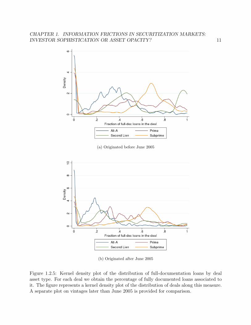
1.2.5 Kernel density plot of the distribution of full-documentation loans by dealasset type. For each deal we obtain the percentage of fully documented loansassociated to it. The figure represents a kernel density plot of the distributionof deals along this measure. A separate plot on vintages later than June 2005is provided for comparison. . . . . . . . . . . . . . . . . . . . . . . . . . . . 11
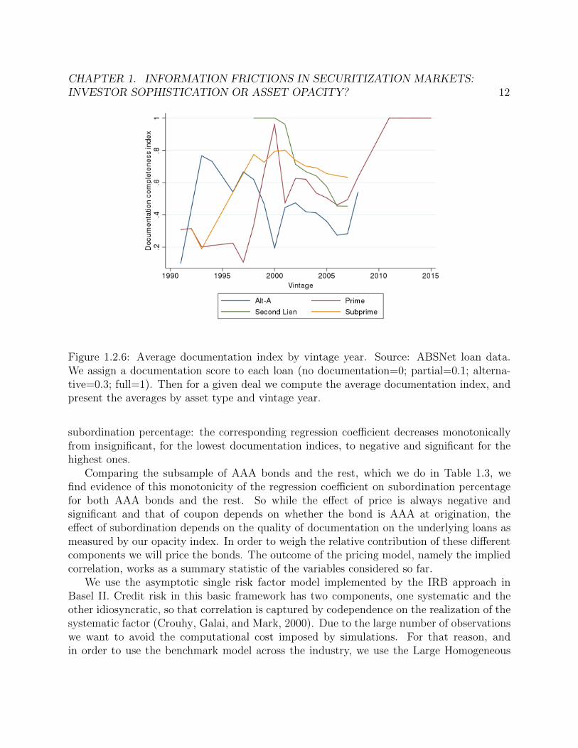
1.2.6 Average documentation index by vintage year. Source: ABSNet loan data.We assign a documentation score to each loan (no documentation=0; par-tial=0.1; alternative=0.3; full=1). Then for a given deal we compute theaverage documentation index, and present the averages by asset type andvintage year. . . . . . . . . . . . . . . . . . . . . . . . . . . . . . . . . . . . 12

iv
1.3.1 Sensitivity of a simulated CMO structure to default correlations. We plotthe expected payoff within a given tranche, for each value of the underlyingcorrelation ρ (parameters are PD=5% and LGD=50% as in Coval, Jurek,and Stafford, 2009a). The results are normalized by baseline estimate, basedon the same parameters and a correlation ρ = 20%. No prepayments areincorporated (i.e. SMM=0%) for comparability of outcomes. . . . . . . . . . 16
1.3.2 Marginal and cumulative prepayment rates implied from the model (1.11), assummarized in Table 1..12. Using loan covariates at origination, prepaymenthazard rates are computed at the loan level. Averages are computed by assettype and month after origination, and plotted here. . . . . . . . . . . . . . . 20
1.3.3 Probability of default implied from the complementary log-log model, es-timates of which are in Table 1..12. Using loan covariates at origination,default probabilities are computed at the loan level. Averages are computedby asset type and month after origination, and plotted here. . . . . . . . . . 21
1.4.1 Average correlation plotted against tranche subordination percentage, on twogiven dates. We use the sample of early vintage bonds (originated prior toJune 2005). Subordinations are assigned to 10 equally spaced bins. Withineach subordination bin we plot the average correlation, along with verticalwhiskers representing the standard error of the average. . . . . . . . . . . . 24
1.4.2 Performance of early vintage tranches: average implied correlation and av-erage rating for bonds originated before June 2005. For a given we computethe implied correlation, at each point in time. The average is taken by trans-action period, by coarse rating at origination (AAA=1,..., BBB=4,..., D=8). 25
1..1 Number of tranches and amount issued by vintage year for private labelcollateralized mortgage obligations. Source: ABSNet bond data. For oursample of early vintages (prior to June 2005) we provide the distribution by(coarse, see Table 1..20) initial rating. . . . . . . . . . . . . . . . . . . . . . 31
1..2 Average tranche price by age of the bond in months. For our sample of bondsoriginated in 2004 and 2005 we compute the average price by the time elapsed(in months) since the bond issue. Vertical whiskers show the standard errors. 36
1..3 Average subordination difference between AAA and BBB bonds. Source:ABSNet bond data.The figure presents the difference between the averageAAA and average BBB subordination over trading time (for early vintages,prior to June 2005) using the rating at the given trading time. The differenceis computed by asset type. . . . . . . . . . . . . . . . . . . . . . . . . . . . 38
1..4 Probability of default by vintage year. We compute the default rate for eachof the deals that compose our population, and then average by vintage yearand asset type. The results are presented here along with standard errorbands around the average. . . . . . . . . . . . . . . . . . . . . . . . . . . . . 39
1..5 Percentage loss given default by vintage year. The aggregate loss given de-fault is computed from the sample of loans associated to the deals that com-pose our population of CMOs. . . . . . . . . . . . . . . . . . . . . . . . . . 40

v
1..6 Average class balance factor by asset class over tranche age. Alongside theaverages, we compute the balance factor that results from a 150% paymentschedule alone (excluding planned amortization). . . . . . . . . . . . . . . . 41
1..7 Standard Prepayment Model of The Bond Market Association. Prepaymentpercentage for each month in the life of the underlying mortgages, expressedon an annualized basis. . . . . . . . . . . . . . . . . . . . . . . . . . . . . . 41
1..8 Plot of average class factor against tranche age by tranche initial rating. . . 421..9 Average realized and weighted average life by coarse rating and asset type.
The second panel includes observations where we found a matching WAL inBloomberg. . . . . . . . . . . . . . . . . . . . . . . . . . . . . . . . . . . . . 43
1..10 Proportion of ARM loans by vintage and asset type. . . . . . . . . . . . . . 441..11 Number of deals originated by asset type and vintage year. . . . . . . . . . 441..12 Histogram plotting all outcomes from the pricing model. . . . . . . . . . . . 451..13 Average correlation plotted against tranche subordination percentage, on two
given dates. We use the sample of early vintage bonds (originated prior toJune 2005). Subordinations are assigned to 10 equally spaced bins. Withineach subordination bin we plot the average correlation, along with verticalwhiskers representing the standard error of the average. . . . . . . . . . . . 46
1..14 Average correlation plotted against tranche subordination percentage, on twogiven dates. Subordination values are assigned to 10 equally spaced bins.Within each subordination bin we plot the average correlation, along withvertical whiskers representing the standard error of the average. . . . . . . . 47
1..15 Distribution of covariates over time (vintage year). . . . . . . . . . . . . . . 481..16 Distribution of covariates over time (vintage year). . . . . . . . . . . . . . . 481..17 Average correlation plotted against tranche subordination percentage, on two
given dates. We use the sample of early vintage bonds (originated prior toJune 2005). Subordinations are assigned to 10 equally spaced bins. Withineach subordination bin we plot the average correlation, along with verticalwhiskers representing the standard error of the average. . . . . . . . . . . . 54
1..18 Tranche balance and number of bonds outstanding by transaction year andmonth. . . . . . . . . . . . . . . . . . . . . . . . . . . . . . . . . . . . . . . 55
2.2.1 Frequency of participants extracting 8 units (Full extraction) and 1 units(Full cooperation) of the CPR during the baseline rounds. . . . . . . . . . . 64
2.2.2 Average individual extraction over time . . . . . . . . . . . . . . . . . . . . 642.3.1 log(MSE) as a function of λ. . . . . . . . . . . . . . . . . . . . . . . . . . . 662.3.2 Observed distribution of choice outcomes and QRE distribution . . . . . . . 66

vi
2.5.1 Heterogeneity of real level extraction of the CPR in the game all CPR usersvs. students (N = 1095). The solid line shows the % time that the Self-regarding NE
was chosen in the game by the Students sample. The round-dot line shows the case with
individuals who use 0% of the real CPR. The square-dot line shows the average level of
extraction in the game by individuals who use 50% of the real CPR. The long-dashed line
the average level of extraction in the game by individuals who use 100% of the real CPR.
The difference in means in the last round is significant at 10%. . . . . . . . . . . . . 762..1 Timeline of the CPR game . . . . . . . . . . . . . . . . . . . . . . . . . . . 822..2 Baseline: behavior over rounds for Pure Self-regarding and Pure cooperator 83
List of Tables
1.1 Regression results from running logit regression 1.1 by maximum likelihood,controlling for vintage year, for vintages up to June 2005. The dependentvariable is a dummy indicator for whether there was a downgrade by Decem-ber 2009. Independent variables include price, subordination, coupon andcoarse rating dummy indicator at the time of the first transaction. The de-pendent variable is the downgrade indicator. Column (1) includes all issues;columns (2) and (3) split the sample between bonds rated AAA at originationand the rest, respectively. Errors are clustered at deal level. . . . . . . . . . 13
1.2 Regression results from running logit specification 1.12 by maximum likeli-hood, controlling for vintage year, for vintages up to June 2005. The depen-dent variable is a dummy indicator for whether there was a downgrade byDecember 2009. Independent variables include price, subordination, couponand coarse rating dummy indicator at the time of the first transaction. Thedependent variable is the downgrade indicator. Each column presents theresults on a subset of the data corresponding to the average documentationindex corresponding to the given deal. Errors are clustered at deal level. . . 14
1.3 Regression results from running logit specification 1.12 by maximum likeli-hood, controlling for vintage year, for vintages up to June 2005. The depen-dent variable is a dummy indicator for whether there was a downgrade byDecember 2009. Independent variables include price, subordination, couponand coarse rating dummy indicator at the time of the first transaction. Thedependent variable is the downgrade indicator. Each column presents theresults on a subset of the data corresponding to the average documentationindex corresponding to the given deal. Errors are clustered at deal level. . . 15

vii
1.4 Regression results from running logit regression 1.12 by maximum likelihood,controlling for vintage year (vintages up to June 2005) and model-impliedprobability of default, as estimated in subsection 1.3. The dependent variableis a dummy indicator for whether there was a downgrade by December 2009.Independent variables include correlation and coarse rating dummy indicatorat the time of the first transaction. The dependent variable is the downgradeindicator. Column (1) includes all issues; columns (2) and (3) split the samplebetween bonds rated AAA at origination and the rest, respectively. Errorsare clustered at deal level. . . . . . . . . . . . . . . . . . . . . . . . . . . . . 27
1.5 Regression results from running logit specification 1.12 by maximum likeli-hood, controlling for vintage year (vintages up to June 2005) and model-implied probability of default as estimated in subsection 1.3. The dependentvariable is a dummy indicator for whether there was a downgrade by De-cember 2009. Independent variables include implied correlation and coarserating dummy indicator at the time of the first transaction. The dependentvariable is the downgrade indicator. Each column presents the results on asubset of the data corresponding to the value of the documentation indexcorresponding to the given deal. Errors are clustered at deal level. . . . . . 28
1.6 Regression results from running logit specification 1.12 by maximum likeli-hood, controlling for vintage year (vintages up to June 2005) and model-implied probability of default as estimated in subsection 1.3. The dependentvariable is a dummy indicator for whether there was a downgrade by De-cember 2009. Independent variables include implied correlation and coarserating dummy indicator at the time of the first transaction. The dependentvariable is the downgrade indicator. Each column presents the results on asubset of the data corresponding to the value of the documentation indexcorresponding to the given deal. Errors are clustered at deal level. . . . . . 29
1..7 Issued amounts and counts by asset type. . . . . . . . . . . . . . . . . . . . 311..8 Subordination percentage by tranche rating - comparison. The figures com-
puted using ABSNet data are derived by aggregating the subordination per-centages at orgination as given in Table 1.2.4. Our sample contains only earlyvintages (prior to June 2005) while Cordell, Huang, and Williams, 2012 uselate vintages as well. . . . . . . . . . . . . . . . . . . . . . . . . . . . . . . . 32
1..9 Origination amounts and counts at origination, by vintage year, comparedto the sample in Adelino, 2009. . . . . . . . . . . . . . . . . . . . . . . . . . 32
1..10 Liquidation rates from the loan sample. Column (1) calculates the percentageof loans linked to early vintage deals (before June 2005) that are liquidated.Column (2) calculates the same ratio for late vintage loans. . . . . . . . . . 32

viii
1..11 This table shows estimates using the maximum likelihood estimation of thecomplementary log-log specification in (1.11), using a nonparametric base-line hazard, on the loan level data available from ABSNet for private labelloans (purchases only). The model treats competing risks independently, in-dicating 1 for failure and 0 for censoring. Each coefficient is the effect of thecorresponding variable on the log hazard rate for either the default or pre-payment of a mortgage. The conditional hazard is captured by performancemonth dummies, where performance is tracked over the first 60 months ofthe sample. The sample is truncated at December 2004 for columns (1) and(2), and at June 2007 for columns (3) and (4). Errors are clustered at CBSAlevel. . . . . . . . . . . . . . . . . . . . . . . . . . . . . . . . . . . . . . . . 33
1..12 This table shows estimates using the maximum likelihood estimation of acomplementary log-log specification, using a hazard specification for prepay-ments and a dummy indicator for default, on the loan level data availablefrom ABSNet for private label loans (purchases only). The hazard modeltreats default risk as censored. Each coefficient is the effect of the correspond-ing variable on the log hazard rate for prepayment or the log probability ofdefault of a mortgage. The conditional hazard is captured by performancemonth dummies, where performance is tracked over the first 60 months ofthe sample. The sample is truncated at December 2004. . . . . . . . . . . . 34
1..13 This table shows estimates using the maximum likelihood estimation of acomplementary log-log specification, using a dummy indicator for default, onthe loan level data available from ABSNet for private label loans (purchasesonly). For each year, variables are taken at the measurement point (eitherdefault time, if defaulted, or observation time, which is the end of the givenyear). . . . . . . . . . . . . . . . . . . . . . . . . . . . . . . . . . . . . . . . 35
1..14 Regression results from running a linear regression at deal level of AAAorigination (as share of total) on the deal opacity index. Controls includemodel-implied PD, vintage year (we include vintages up to June 2005) andasset type. . . . . . . . . . . . . . . . . . . . . . . . . . . . . . . . . . . . . 36
1..15 Regression results from running logit regression 1.12 by maximum likelihood,controlling for vintage year (vintages up to June 2005) and model-impliedprobability of default, as estimated in subsection 1.3. The dependent variableis a dummy indicator for whether there was a downgrade by December 2009.Column (1) includes all issues; columns (2) and (3) split the sample betweenbonds rated AAA at origination and the rest, respectively. Independentvariables include deal level average correlation (column 1), AAA averagecorrelation (column 2), sub-AAA average correlation (column 3) and coarserating dummy indicator at the time of the first transaction. The dependentvariable is the downgrade indicator. Errors are clustered at deal level. . . . 37

ix
1..16 Regression results from running logit specification 1.12 by maximum likeli-hood, controlling for vintage year (vintages up to June 2005) and model-implied probability of default as estimated in subsection 1.3. The dependentvariable is a dummy indicator for whether there was a downgrade by Decem-ber 2009. Independent variables include deal level average implied correlationand coarse rating dummy indicator at the time of the first transaction. Thedependent variable is the downgrade indicator. Each column presents the re-sults on a subset of the data corresponding to the value of the documentationindex corresponding to the given deal. Errors are clustered at deal level. . . 49
1..17 Regression results from running logit specification 1.12 by maximum likeli-hood, controlling for vintage year (vintages up to June 2005) and model-implied probability of default as estimated in subsection 1.3. The dependentvariable is a dummy indicator for whether there was a downgrade by De-cember 2009. Independent variables include AAA average correlation (upperpanel), sub-AAA average correlation (lower panel) and coarse rating dummyindicator at the time of the first transaction. The dependent variable is thedowngrade indicator. Each column presents the results on a subset of thedata corresponding to the value of the documentation index correspondingto the given deal. Errors are clustered at deal level. . . . . . . . . . . . . . . 50
1..18 Regression results from running a linear regression at deal level of AAAorigination (as share of total) on the deal opacity index. Controls includemodel-implied PD, vintage year (we include vintages up to June 2005) andasset type. . . . . . . . . . . . . . . . . . . . . . . . . . . . . . . . . . . . . 51
1..19 Data cleaning stages with number of tranches outstanding at the end of eachstep. . . . . . . . . . . . . . . . . . . . . . . . . . . . . . . . . . . . . . . . . 51
1..20 Mapping of ratings - fine and coarse level (with numbering code) . . . . . . 521..21 Liquidation rates from the loan sample, and PD used for baseline estimation.
Column (1) calculates the percentage of loans linked to early vintage deals(before June 2005) that are liquidated. Column (2) calculates the same ratiofor late vintage loans. Column (3) shows the PD parameters used for thepricing model, calculated as the average of the deal level liquidation rates forboth early and late deals. . . . . . . . . . . . . . . . . . . . . . . . . . . . . 52
1..22 Regression results from running logit regression 1.12 by maximum likelihood,controlling for vintage year, for vintages up to June 2005. The dependentvariable is a dummy indicator for whether there was a downgrade by De-cember 2009. Independent variables include correlation and coarse ratingdummy indicator at the time of the first transaction. The dependent vari-able is the downgrade indicator. Column (1) includes all issues; columns (2)and (3) split the sample between bonds rated AAA at origination and therest, respectively. Errors are clustered at deal level. . . . . . . . . . . . . . . 53

x
1..23 Regression results from running logit specification 1.12 by maximum likeli-hood, controlling for vintage year, for vintages up to June 2005. The depen-dent variable is a dummy indicator for whether there was a downgrade byDecember 2009. Independent variables include implied correlation and coarserating dummy indicator at the time of the first transaction. The dependentvariable is the downgrade indicator. Each column presents the results on asubset of the data corresponding to a given asset type. Errors are clusteredat deal level. . . . . . . . . . . . . . . . . . . . . . . . . . . . . . . . . . . . 53
1..24 Regression results from running logit specification 1.12 by maximum likeli-hood, controlling for vintage year, for vintages up to June 2005. The de-pendent variable is a dummy indicator for whether there was a downgradeby December 2009. Independent variables include implied correlation andcoarse rating dummy indicator at the time of the first transaction. Thedependent variable is the downgrade indicator. Each column presents theresults on a subset of the data corresponding to the average documentationindex corresponding to the given deal. Errors are clustered at deal level. . . 55
1..25 Regression results from running logit specification 1.12 by maximum likeli-hood, controlling for vintage year, for vintages up to June 2005. The de-pendent variable is a dummy indicator for whether there was a downgradeby December 2009. Independent variables include implied correlation andcoarse rating dummy indicator at the time of the first transaction. Thedependent variable is the downgrade indicator. Each column presents theresults on a subset of the data corresponding to the average documentationindex corresponding to the given deal. Errors are clustered at deal level. . . 56
1..26 Regression results from running the panel regression 1.13, by GLS withtranche random effects. The first line gives the coefficient for the changeover 1 month (lagged 1 month) of the correlation coefficient, and the sec-ond one the coefficient for the change over 1 month (lagged 1 month) of thechange in rating (in notches). Errors are clustered at deal level. . . . . . . . 57
1..27 Regression results from running the panel regression 1.13, by GLS withtranche random effects. The first line gives the coefficient for the changeover 1 month (lagged 1 month) of the correlation coefficient, and the sec-ond one the coefficient for the change over 1 month (lagged 1 month) of thechange in rating (in notches). Errors are clustered at deal level. . . . . . . . 58
2.1 Comparison of model performance by number of types - CPR users sample 732.2 Comparison of model performance by number of types - Student sample . . 732.3 Type classification and structural parameters - CPR users and students . . 742.4 Class-conditional probability of choice . . . . . . . . . . . . . . . . . . . . . 752.5 Drivers of class share - real CPR user sample . . . . . . . . . . . . . . . . . 762..1 Labs in the field . . . . . . . . . . . . . . . . . . . . . . . . . . . . . . . . . 802..2 Table points of the CPR game. . . . . . . . . . . . . . . . . . . . . . . . . . 81

xi
2..3 Real Users’ Socio-economic Characteristics . . . . . . . . . . . . . . . . . . 822..4 Class share determinants (student sample) without the restrictions coming
from the real CPR users’ model . . . . . . . . . . . . . . . . . . . . . . . . . 832..5 Class share determinants (student sample) without any restrictions . . . . . 832..6 Class share determinants (real CPR user sample) without any restrictions . 84

xii
Acknowledgments
I gratefully acknowledge the contribution each of my committee members, Shachar Kariv,Amir Kermani, Christopher Palmer and Nancy Wallace, have brought to this dissertation:In particular I thank Nancy Wallace, for the time she spent teaching me and discussing myprojects. I thank Shachar Kariv for showing me the four essential tradeoffs faced by eco-nomic agents. I thank Christopher Palmer for being a role model. I am grateful to NicolaeGarleanu and Panos Patatoukas for their teachings and their support.
God and my family have been my strength and source of support. My eternal gratitudeto my wife and coauthor, Sandra, without whom I would not have made it. My daughtersCristina and Teresa are my joy and my purpose. To my father, German, my gratitude forhis example not only as a father but also as an entrepreneur, ready to face with an openheart the risks and the costs of innovation.
I thank my colleagues and friends for their contribution to making the PhD a happy time,especially my journey companions Carlos Avenancio, Al Hu and Sheisha Kulkarni. A specialmention to my friends Andy Chen, Connie Fontanoza, Irfan Hafeez, Haoyang Liu, Fr. JesseMontes, An Nguyen, Sean Roche, Ivan Villasenor and Dayin Zhang.
I am grateful to the members of the Haas community who have helped me along the way.I thank Tom Chappelear, Kim Guilfoyle, Melissa Hacker, Paulo Issler and Charles Montague.
Financial assistance from Haas School of Business, the Fisher Center for Real Estate andUrban Economics and the Xlab is gratefully acknowledged.

1
Chapter 1
Information Frictions in SecuritizationMarkets: Investor Sophistication orAsset Opacity?
Because the central premise of securitization is diversification through pooling, default cor-relations are crucial to bondholders. Hence prices of structured products that are subjectto default risk reveal investors’ beliefs about correlations. Higher correlations imply morevolatility of the portfolio cashflows, which is valuable to subordinate bondholders but detri-mental to senior ones (Duffie and Garleanu, 2001). Yet there is still a lack of attention todefault correlations -which Duffie, 2008 deems the “weak link” in the pricing of collateralizeddebt obligations (CDO)- relative to the attention given to default probabilities.
Coval, Jurek, and Stafford, 2009a1 show that bond prices are sensitive to underlyingdefault correlations, and that this sensitivity compounds along the structured finance chain.As (Cordell, Huang, and Williams, 2012) show (see Figure 1.0.1) the underlying collateralof cash CDOs is predominantly mezzanine tranches of collateralized mortgage obligations(CMO). This means that in practice CDOs behave -with respect to the underlying loans- theway CDO2 behave in Coval, Jurek, and Stafford, 2009a. Thus Coval, Jurek, and Stafford,2009a highlight the importance of CMO default correlations, while leaving the question openas to which investors are miscalculating them.
To calculate impleid correlations I use the pricing model that Hull and White, 2006 call“the standard market model for valuing collateralized debt obligations and similar instru-ments”, namely a single factor Gaussian copula (Li, 2000).2 I estimate the probability ofdefault (PD) and loss given default (LGD) from loan performance data, following common
1Our estimate of default correlation uses the same method as they do. Using their parameters I replicatetheir results (see Figure 1.3.1).
2See also Brunne, 2006; D’Amato and Gyntelberg, 2005; Duffie and Singleton, 2012; Elizalde, 2005;Hull and White, 2004; Hull and White, 2006; Hull and White, 2008; McGinty et al., 2004; Tzani andPolychronakos, 2008.

CHAPTER 1. INFORMATION FRICTIONS IN SECURITIZATION MARKETS:INVESTOR SOPHISTICATION OR ASSET OPACITY? 2
Figure 1.0.1: Diagram: from loans to RMBS CMO, from CMO to CDO, from CDO toCDO2. Details are reported on the total number of loans recorded by ABSNet, the universeof securities issued and the average subordination percentage by Standard & Poor’s rating,as explained in Section 1.2
practice in CDO pricing models that PD and LGD on the underlying asset are taken asgiven, and correlations are directly implied from market prices of the bonds.
In order to understand which investors were informed I look at the information contentrevealed by market prices. I say that implied correlations are informative to the extentthat they predict subsequent bond downgrades, controlling for agency rating at the time oftransaction. I find that early prices of CMOs (i.e. prior to the pre-crisis mortgage boomthat took place after June 2005) are informative, results which are in line with those ofAshcraft et al., 2011. Adelino, 2009 argues that this information content is absent from AAAtranches, implying the existence of an information differential between the unsophisticatedsenior investor and the sophisticated junior one (Boot and Thakor, 1993). In Gorton andPennacchi, 1990, the former seeks information-insensitive tranches (in particular the AAArated) while the latter can handle the information-sensitive ones (the junior tranches).3
I show that the presence of this information differential is essentially conditioned by thequality of the documentation on the underlying loans. More specifically, correlations implied
3The efficiency of this arrangement is discussed by Dang, Gorton, and Holmstrom, 2013. In particular,when information is costly this helps the market liquidity (Gorton and Ordonez, 2013).

CHAPTER 1. INFORMATION FRICTIONS IN SECURITIZATION MARKETS:INVESTOR SOPHISTICATION OR ASSET OPACITY? 3
from junior tranches are no more informative than those of AAA tranches for “low-doc deals,where the value of the asset is opaque. Conversely, AAA correlations are no less informativethan junior ones within “full-doc deals, which are not opaque. Thus errors in computingdefault correlations in the running to the crisis were not the problem of AAA investors,but rather a problem of “low-doc” investors. Information deficiencies were thus essentiallydriven by the opacity of the underlying assets, which I capture through the completeness ofdocumentation.
Some evidence remains that differential information exists in deals with intermediatelevels of documentation. This shows that the agency problem between senior and juniorinvestors remains, and that sophistication matters for intermediate opacity degrees. Ashcraftand Schuermann, 2008 argue there are two key information frictions between the investorand the originator of the securities. The first one, lack of investor sophistication, gives rise todifferential information and eventually a principal-agent problem. This has been the mainfocus of the literature, as discussed so far. The second information friction, lack of duediligence about the quality of the assets, entails an incomplete information problem thatconstitutes the focus of this paper. The main contribution of this paper is to show howthe two frictions highlighted by Ashcraft and Schuermann, 2008 interact, arguing that assetopacity has precedence over investor sophistication.
The results suggest that regulation interventions focusing on the agency problem, such asrisk retention in the form of skin in the game, can be complemented by market transparencyinitiatives -achieving better documentation on the underlying loans-. To the extent thatthe incomplete information problem is easier to solve than differential information one, suchtransparency initiatives can be an effective instrument.
As explained in IOSCO, 2008 the key step in the rating process of a structured productis to determine the amount of subordination that will ensure a given rating, in particular aStandard & Poor’s AAA. This makes the subordination structure an essential aspect of thebondholder’s risk assessment, which yields alone do not reflect. Implied correlation aggre-gates yield and subordination percentage, taking into account the subordination structuretogether with the default and prepayment risk of the underlying loans.
Between yield and subordination, the latter seems to be the one whose informationcontent is most sensitive to asset opacity. Whereas the informativeness of bond price does notvary much as a function of documentation completeness, that of the tranche subordinationdoes. A fall in price is uniformly predictive of a downgrade, even controlling for rating.Instead, subordination is only predictive of downgrades for well documented deals. In linewith this I find evidence that, controlling for probability of default, the amount of AAAissuance is decreasing in documentation completeness. The result is consistent with Skretaand Veldkamp, 2009, whose theory predicts that ratings are more likely to be inflated whenassets are opaque.
The paper proceeds as follows. Section 1.1 relates this paper to the literature. Section 1.2presents our data. Section 2.4 explains the copula model we use to infer default correlations.Section 1.4 presents the model estimates on our panel data. Section 1.5 lays out regressionsto analyze the relative information content of ratings and prices. Section 1.6 concludes.

CHAPTER 1. INFORMATION FRICTIONS IN SECURITIZATION MARKETS:INVESTOR SOPHISTICATION OR ASSET OPACITY? 4
1.1 Literature
Low documentation loans give rise to opaque deals. From the loan level data on documen-tation completeness I construct an index of deal opacity. A number of papers have studiedopacity in mortgage markets. JEC, 2007 documents a relative decline in the number of fulldocumentation subprime loans in the running to the crisis. Keys et al., 2010 argue that the“low-doc” loans underperformed (in terms of defaults) relative to otherwise similar but bet-ter documented loans. This underperformance of low-doc loans is confirmed by the results ofKau et al., 2011. Moreover,Ashcraft, Goldsmith-Pinkham, and Vickery, 2010 use a loan-levelmeasure of documentation completeness (similar to the one we use) to document the under-performance of “low-doc” deals. While our results are consistent with theirs in the sense ofunderperformance of low-doc deals, the performance we emphasize is on the information con-tent reflected in market transactions. Finally, AdelinoGerardiHartmanGlaser:16 findthat investors deal with opacity by skimming the underlying loans; they look at the time tosale of loans in the secondary market, while we consider the channel of bond prices.
The collapse of CDO ratings after the crisis was arguably linked to subjective ratings(Griffin and Tang, 2012) and rating inflation (Benmelech and Dlugosz, 2010). Skreta andVeldkamp, 2009 argue that rating inflation worsens when assets are opaque, or “complex” touse their term (complexity being defined as the level of uncertainty about the true securityvalue). We empirically corroborate their prediction that, controlling for risk attributes,low-doc deals see relatively more AAA issuance.
Disagreement is the starting point for differential information in market prices. By takingdefault probabilities as fixed and estimating default correlations, the implicit assumption inthe Gaussian copula approach is that the main source of disagreement among investors in agiven deal is the default correlation. The literature has examined the role of disagreementabout other risk attributes such as prepayment speed (Carlin, Longstaff, and Matoba, 2014;Diep, Eisfeldt, and Richardson, 2016) or the probability of a crisis (Simsek, 2013). Theprominence of Gaussian copulas in the CDO literature suggests that the primary source ofdisagreement across bonds in such a structure is the default correlation.
Default correlations can be inferred from default experience instead of from asset values.This is the approach followed by Cowan and Cowan, 2004; Servigny and Renault, 2002;Geidosh, 2014; Gordy, 2000; Nagpal and Bahar, 2001. By construction these estimatorsare more tightly linked to realized defaults than even the updated value of price-impliedcorrelations. Though default-based measures are not directly comparable to ours (Frye,2008), one study based on default experience worth noting here is Griffin and Nickerson,2016. They infer rating agency beliefs about corporate default correlations by studyingcollateralized loan obligation (CLO). Their results suggest such beliefs were revised upwardsafter the crisis, but not sufficiently so when benchmarked against a default experience-basedestimator accounting for unobserved frailty in the default generating process (Duffie et al.,2009). For our part we document that agency ratings adapted more slowly to the crisis thanmarket prices.

CHAPTER 1. INFORMATION FRICTIONS IN SECURITIZATION MARKETS:INVESTOR SOPHISTICATION OR ASSET OPACITY? 5
The literature has historically attributed default clustering to joint dependence on a sys-tematic shock (Bisias et al., 2012; Chan-Lau et al., 2009; Bullard, Neely, and Wheelock,2009; Khandani, Lo, and Merton, 2013). We have followed this approach, using a Gaussiancopula. Recent literature distinguishes two additional sources of default clustering: unob-served frailty (Duffie et al., 2009; Kau, Keenan, and Li, 2011; Griffin and Nickerson, 2016)and contagion (see appendix 1.6).4 In particular Azizpour, Giesecke, and Schwenkler, 2016;Gupta, 2016 and Sirignano, Sadhwani, and Giesecke, 2016 suggest the contagion channel isimportant. In light of this literature, this paper is the first of several steps to understandwhich sources of default clustering are priced in mortgage markets.
1.2 Data
ABSNet collects monthly information about private label securitization deals, providingsnapshots of all tranches inside a given deal between the time of origination and the endof 2016. For each month it provides updated information on rating, subordination, bondmaturity and coupon. We collect all the snapshots available from each deal in their website.The tranches in their data are organized in a matrix format by increasing attachment point.From there we derive the detachment point for each tranche, and thus the waterfall of lossesfor the given deal.5
Between early cohorts (i.e. originated before June 2005) and late ones, we observe 71,915tranches (linked to 5,790 deals, roughly 14 tranches per deal on average) for a total $4,380.3bnof originated securities.6 Alt-A and subprime deals are the largest classes (see Table 1..7)which mostly built up in the running to the crisis (Gorton, 2009). Our estimation sample,composed of the 35,692 tranches issued before June 2005, is also composed mostly of suprimeand Alt-A bonds, though the proportion is smaller than it is among late vintages.
CMOs are traded over the counter. Our price data comes from Thomson Reuters, whichrecords the bid price and the mid from January 2004 onwards.7 It only covers the series ofprices for CMOs originated before and up to June 2005. Starting July 2009, our ABSNet alsorecords transaction prices over time. Matching the two sources on CUSIP, year and month(keeping the nearest transaction to the rating observation date8) we check the consistencybetween the ABSNet price and the mid price in Thomson Reuters. We find a median absolutedifference is $0.06 and a 99th percentile of $1.51, the difference being consistent with timedifferences in the date of the observation across sources. Between the two sources we have
4For a review of recent literature on contagion see Bai et al., 2015.5Some deals have more than one structure inside, each structure giving rise to its own subordination
waterfall. We source each structure separately, and treat different structures as we would different deals.6Adelino, 2009, uses 67,412 securities from JP Morgan’s MBS database, for a total issue of $4,204.8bn
(ours also includes post-crisis issuance). See Table 1..9. We follow his data cleaning procedures such asremoving Interest Only, Principal Only, Inverse Floater and Fixed to Variable bonds from the sample.
7There is little variation in the spread (measured as the difference between the mid and the bid). Theaverage is $0.17 on a par price of $100. The median is $0.06, same as the 25th and 75th percentiles.
8The average distance in days is 1.83, the median is 0 and the 99th percentile 53 days

CHAPTER 1. INFORMATION FRICTIONS IN SECURITIZATION MARKETS:INVESTOR SOPHISTICATION OR ASSET OPACITY? 6
(a) Number of tranches (b) Total issue
Figure 1.2.1: Number of tranches and amount issued by vintage year for private label col-lateralized mortgage obligations. Source: ABSNet bond data. The counts in our estimationsample (early vintages, prior to June 2005) are recorded in blue, while the numbers for latevintage tranches are illustrated in light grey.
a data gap, whereby for late (post 2005) cohorts we only have post crisis prices (after July2009). For early cohorts, instead, we can track prices over time (the data provides as frequentas daily trading prices). Hence we will conduct the main analyses on the early cohorts.
The majority of issues in our sample are rated AAA, especially in terms of amount (seeFigure 1..1). As Figure 1..2 shows, the bonds were mostly priced at par, or even slightpremium, at the moment of origination, which we observe for the tranches originated in2004 and 2005. This applies in particular to BBB bonds, which Deng, Gabriel, and Sanders,2011 link to demand pressures from the surge of CDO markets. Within two months of issueprices have dropped and the variation in prices increased. Bonds then remain priced at adiscount over subsequent trades. As Figure 1.2.2 shows, discounts are higher in the runningto the crisis for AAA bonds, and within AAA they are higher for prime and Alt-A bonds.Over 2007 we see prices fall, but BBB bonds see a sharp fall compared to the relativelymild fluctuation in AAA prices. In comparison, AAA and BBB bond coupons have a similarpattern over time as shown by Figure 1.2.3. Aside from the wider fluctuations for BBBsubprime and second lien bonds compared to the corresponding AAA ones, the differenceover time across seniorities is less over prices than over coupons.
We now look at the deal subordination structure in our data. ABSNet provides theStandard & Poor’s (S&P) rating, which is the main ordinal variable we use to capture thecash flow sequence among the bonds in a given deal. When the security has no S&P ratingwe use the one issued by Fitch, which uses the same grading scale. Figure 1.2.4 shows theaverage subordination percentage by rating at origination. Tranching becomes steeper as therating increases, and Second Lien/Subprime deals in general require more subordination at

CHAPTER 1. INFORMATION FRICTIONS IN SECURITIZATION MARKETS:INVESTOR SOPHISTICATION OR ASSET OPACITY? 7
(a) Tranches rated AAA at origination
(b) Tranches rated BBB at origination
Figure 1.2.2: Average price by initial rating. Source: Thomson Reuters. For all the pricesobserved within a given month we use the closest to month end. The figure presents averageprice over trading time (for early vintages, prior to June 2005) controlling for initial rating.

CHAPTER 1. INFORMATION FRICTIONS IN SECURITIZATION MARKETS:INVESTOR SOPHISTICATION OR ASSET OPACITY? 8
(a) Tranches rated AAA at origination
(b) Tranches rated BBB at origination
Figure 1.2.3: Average coupon by initial rating. Source: ABSNet bond data.The figurepresents average coupon rate over trading time (for early vintages, prior to June 2005)controlling for initial rating.

CHAPTER 1. INFORMATION FRICTIONS IN SECURITIZATION MARKETS:INVESTOR SOPHISTICATION OR ASSET OPACITY? 9
each rating grade. The average tranching structure lines up in general with the one Cordell,Huang, and Williams, 2012 obtain from Intex data (see Table 1..8 for a comparison), apartfrom relatively thicker AAA tranches in our sample. Intex contains data on so-called 144Adeals,9 which are not in our sample, aside from late vintage issues which are also excludedfrom our sample.
Figure 1.2.4: Deal structure. Source: ABSNet bond data. For our sample of early vintagedeals, we look at the difference in subordination between tranches with consecutive S&Pratings. We then average the outcome by rating and asset type, aggregating at coarse gradelevel (see mapping in Table 1..20). This average difference is represented here, stacked byasset type.
Changes in subordination percentage take place over the cycle, though mostly for sub-prime deals. This is shown in Figure 1..3, which depicts the point-in-time difference inaverage subordination between AAA and BBB tranches. While the difference remains closeto constant for Alt-A and prime deals, the difference rises for subprime deals in the runningto the crisis, with a slight downward trend over time afterwards. In summary, among thetranche-level variables we use for the pricing model, i.e. price, coupon and subordinationstructure, the first two show exhibit more cyclical variation than the latter.
Besides the bond level data, we have loan origination and performance data on theunderlying loans as recorded by ABSNet. Loans are linked to their respective deals. Westart with a sample of 6,453,799 loans of which 3,509,785 are originated in 2005 or later.We have loan and borrower characteristics such as FICO score, owner occupancy, original
9Rule 144A of the Securities Act of 1933 allows private companies to sell unregistered securities toqualified institutional buyers.

CHAPTER 1. INFORMATION FRICTIONS IN SECURITIZATION MARKETS:INVESTOR SOPHISTICATION OR ASSET OPACITY? 10
loan amount and original LTV, which we will use in Section 1.3 to estimate default andprepayment hazard models.
The loan data also provides a documentation completeness indicator for each loan. Doc-umentation completeness for a given loan is categorized as full, limited, alternative or nodocumentation. Figure 1.2.5 shows a distribution of the share (at the deal level) of loanswith full documentation in our sample of vintages prior to June 2005. It suggests subprimeloans were relatively better documented than Alt-A deals, with densities peaking around 0.7and 0.35 approximately. Prime deals show a higher dispersion in terms of documentationcompleteness. In comparison, density plots on post-June 2005 issues suggest that documen-tation completeness deteriorated more among Alt-A, second lien and prime deals relative tosubprime ones in the running to the crisis.
Including cases of partial and alternative documentation, we assign a documentation scoreto each loan (no documentation=0; partial=0.1; alternative=0.3; full=1). In comparisonKeys et al., 2010 use percentage of completeness, which is equivalent to our index excludingthe intermediate values. Linking loans to deals we average documentation scores into adeal level opacity index. Figure 1.2.6 presents the averages by asset type and vintage year.Note that Alt-A markets can only be characterized by low documentation levels -relative toother types- from year 2000 onwards. The downward slope in Figure 1.2.6 is in line reflectsthe decline in lending standards in the running to the crisis observed on subprime loans byDell’Ariccia, Igan, and Laeven, 2012 and Keys et al., 2010.
Other data include dynamic covariates such as CBSA level home price indices from FHFAand interest rate data; we use the difference between the loan original interest rate -fromABSNet- and the original ten year Treasury rate -from FRED-. Using Treasury rates wealso compute coupon gap (the difference between the ten year rate at origination and thecurrent ten year rate). From Bloomberg we extract bond contractual maturities and weightedaverage life.
1.3 Modelling approach
We start by assessing the information content of different bond attributes considered so far(price, coupon and subordination) by estimating regressions of the form
downgradei,2009 = f(α + βXi0 + ηratingi0 + εi) (1.1)
where Xi0 is a vector of bond attributes at origination such as price, subordination andcoupon, controlling for deal vintage and tranche rating at origination.
Table 1.1 presents regression results for specification (1.1). A higher bond price is pre-dictive of a lower probability of downgrade, and a higher percentage subordination has thesame effect. Both are significant predictors of downgrades. A higher coupon significantlypredicts lower downgrades, though this only holds for below-AAA bonds. Now we splitthe sample by value of the opacity index derived in Section 1.2, using four buckets of size0.25. Table 1.2 shows that the effect most clearly driven by documentation quality is that of
CHAPTER 1. INFORMATION FRICTIONS IN SECURITIZATION MARKETS:INVESTOR SOPHISTICATION OR ASSET OPACITY? 11
(a) Originated before June 2005
(b) Originated after June 2005
Figure 1.2.5: Kernel density plot of the distribution of full-documentation loans by dealasset type. For each deal we obtain the percentage of fully documented loans associated toit. The figure represents a kernel density plot of the distribution of deals along this measure.A separate plot on vintages later than June 2005 is provided for comparison.
CHAPTER 1. INFORMATION FRICTIONS IN SECURITIZATION MARKETS:INVESTOR SOPHISTICATION OR ASSET OPACITY? 12
Figure 1.2.6: Average documentation index by vintage year. Source: ABSNet loan data.We assign a documentation score to each loan (no documentation=0; partial=0.1; alterna-tive=0.3; full=1). Then for a given deal we compute the average documentation index, andpresent the averages by asset type and vintage year.
subordination percentage: the corresponding regression coefficient decreases monotonicallyfrom insignificant, for the lowest documentation indices, to negative and significant for thehighest ones.
Comparing the subsample of AAA bonds and the rest, which we do in Table 1.3, wefind evidence of this monotonicity of the regression coefficient on subordination percentagefor both AAA bonds and the rest. So while the effect of price is always negative andsignificant and that of coupon depends on whether the bond is AAA at origination, theeffect of subordination depends on the quality of documentation on the underlying loans asmeasured by our opacity index. In order to weigh the relative contribution of these differentcomponents we will price the bonds. The outcome of the pricing model, namely the impliedcorrelation, works as a summary statistic of the variables considered so far.
We use the asymptotic single risk factor model implemented by the IRB approach inBasel II. Credit risk in this basic framework has two components, one systematic and theother idiosyncratic, so that correlation is captured by codependence on the realization of thesystematic factor (Crouhy, Galai, and Mark, 2000). Due to the large number of observationswe want to avoid the computational cost imposed by simulations. For that reason, andin order to use the benchmark model across the industry, we use the Large Homogeneous

CHAPTER 1. INFORMATION FRICTIONS IN SECURITIZATION MARKETS:INVESTOR SOPHISTICATION OR ASSET OPACITY? 13
downgrade(1) (2) (3)All AAA only Non-AAA only
Price -0.0187∗∗∗ -0.0457∗∗∗ -0.00932∗∗∗
(0.00151) (0.00299) (0.00149)Coupon -0.123∗∗∗ -0.0365 -0.184∗∗∗
(0.0178) (0.0245) (0.0240)Subordination -3.130∗∗∗ -3.944∗∗∗ -3.978∗∗∗
(0.268) (0.565) (0.310)
Observations 26,242 14,034 12,206Rating at first transaction Y N YVintage year Y Y Y
Standard errors in parentheses∗ p < 0.1, ∗∗ p < 0.05, ∗∗∗ p < 0.01
Table 1.1: Regression results from running logit regression 1.1 by maximum likelihood,controlling for vintage year, for vintages up to June 2005. The dependent variable is a dummyindicator for whether there was a downgrade by December 2009. Independent variablesinclude price, subordination, coupon and coarse rating dummy indicator at the time of thefirst transaction. The dependent variable is the downgrade indicator. Column (1) includesall issues; columns (2) and (3) split the sample between bonds rated AAA at origination andthe rest, respectively. Errors are clustered at deal level.
Gaussian Copula (LHGC) model (Brunne, 2006; D’Amato and Gyntelberg, 2005; Duffie andSingleton, 2012; Elizalde, 2005; McGinty et al., 2004; Tzani and Polychronakos, 2008).10
In the LHGC setup two assumptions apply: all loans in a given pool have the same(known) probability of default PD, and all have the same recovery rate RR. The homogene-ity allows us to abstract from individual loan sizes, which we normalize to one. Consider apool of N mortgages. Default times τ = τ1, . . . , τN are correlated random variables. Cor-relation is captured by the loading on one -exogenous- systematic factor S, which in oursetting follows a standard normal distribution. In the one-factor Gaussian copula case theindividual default probability is given by
p(s, T ) := Pr(τ ≤ T |S = s) = Φ
(Φ−1(PD)−√ρs√
1− ρ
)(1.2)
10Following Li, 2000 the Gaussian copula offered a conceptually simple framework for pricing structuredsecurities,11 which allegedly contributed to investor overconfidence and eventually set the stage for thefinancial crisis in 2007.12

CHAPTER 1. INFORMATION FRICTIONS IN SECURITIZATION MARKETS:INVESTOR SOPHISTICATION OR ASSET OPACITY? 14
(1) (2) (3) (4)[0, 0.25) [0.25, 0.5) [0.5, 0.75) [0.75, 1]
Downgrade indicator
Price -0.0159∗∗∗ -0.0200∗∗∗ -0.0110∗∗∗ -0.0169∗∗∗
(0.00606) (0.00333) (0.00267) (0.00354)Coupon -0.142∗∗ -0.0380 -0.117∗∗∗ -0.0780∗
(0.0640) (0.0304) (0.0441) (0.0466)Subordination 0.00163 -1.857∗∗∗ -4.016∗∗∗ -5.722∗∗∗
(0.864) (0.657) (0.489) (0.943)
Observations 2,489 5,513 7,073 5,049Rating at first transaction Y Y Y YVintage year Y Y Y YAsset type Y Y Y Y
Standard errors in parentheses∗ p < 0.10, ∗∗ p < 0.05, ∗∗∗ p < 0.01
Table 1.2: Regression results from running logit specification 1.12 by maximum likelihood,controlling for vintage year, for vintages up to June 2005. The dependent variable is a dummyindicator for whether there was a downgrade by December 2009. Independent variablesinclude price, subordination, coupon and coarse rating dummy indicator at the time ofthe first transaction. The dependent variable is the downgrade indicator. Each columnpresents the results on a subset of the data corresponding to the average documentationindex corresponding to the given deal. Errors are clustered at deal level.
where PD is the unconditional default probability. Defaults are independent conditional onthe realization of the systematic factor S, i.e.
Pr(τ1 ≤ t, . . . , τN ≤ t|S = s) =N∏k=1
Pr(τk ≤ t|S = s)
which simplifies computations.Total losses from the pool accumulate over time to l(t) = 1
N
∑Nk=1(1 − RR)1(τk≤t). The
losses are distributed along the tranches from the deal. A given tranche’s position in thewaterfall is characterized by its lower and upper attachment points a and b where 0 ≤ a <b ≤ 1. Its notional is a proportion b − a of the total pool notional N . The losses borne bythis tranche are given by
l[a,b](t) =[l(t)− a]+ − [l(t)− b]−
b− a.
This exposure to risk affects the expected payoff of the CMO tranche. Using the recoveryrate, equation (1.2) yields the following estimate of expected losses within the [a, b] tranche

CHAPTER 1. INFORMATION FRICTIONS IN SECURITIZATION MARKETS:INVESTOR SOPHISTICATION OR ASSET OPACITY? 15
(1) (2) (3) (4)
[0, 0.25) [0.25, 0.5) [0.5, 0.75) [0.75, 1]Downgrade indicator - AAA only
Price -0.0352∗∗∗ -0.0360∗∗∗ -0.0347∗∗∗ -0.0539∗∗∗
(0.00900) (0.00529) (0.00632) (0.0127)Coupon 0.0508∗∗∗ 0.0546 0.0919 0.118∗
(0.0161) (0.0451) (0.0575) (0.0625)Subordination -0.0174 -2.774∗∗ -2.014 -9.907∗∗∗
(1.622) (1.229) (1.881) (3.612)Observations 1,325 3,073 3,272 2,926Rating at first transaction Y Y Y YVintage year Y Y Y YAsset type Y Y Y Y
Downgrade indicator - not AAA
Price -0.0163∗∗ -0.0129∗∗∗ -0.00786∗∗∗ -0.0113∗∗∗
(0.00714) (0.00371) (0.00250) (0.00358)Coupon -0.367∗∗∗ -0.167∗∗∗ -0.201∗∗∗ -0.156∗∗∗
(0.102) (0.0475) (0.0529) (0.0603)Subordination -0.309 -2.648∗∗∗ -4.501∗∗∗ -4.193∗∗∗
(1.881) (0.880) (0.538) (0.784)Observations 1,038 2,248 3,757 2,111Rating at first transaction Y Y Y YVintage year Y Y Y YAsset type Y Y Y Y
Standard errors in parentheses∗ p < 0.10, ∗∗ p < 0.05, ∗∗∗ p < 0.01
Table 1.3: Regression results from running logit specification 1.12 by maximum likelihood,controlling for vintage year, for vintages up to June 2005. The dependent variable is a dummyindicator for whether there was a downgrade by December 2009. Independent variablesinclude price, subordination, coupon and coarse rating dummy indicator at the time ofthe first transaction. The dependent variable is the downgrade indicator. Each columnpresents the results on a subset of the data corresponding to the average documentationindex corresponding to the given deal. Errors are clustered at deal level.

CHAPTER 1. INFORMATION FRICTIONS IN SECURITIZATION MARKETS:INVESTOR SOPHISTICATION OR ASSET OPACITY? 16
by payment date Ti:
E[l[a,b](Ti)] =1
b− a
∫ ∞−∞
e−s2/2
√2π
([(1−RR)p(s, Ti)− a]+ − [(1−RR)p(s, Ti)− b]+
)ds (1.3)
Duffie and Garleanu, 2001 and Coval, Jurek, and Stafford, 2009a look at the sensitivityof expected recovery to default correlation. Figure 1.3.1 replicates the exercise in Coval,Jurek, and Stafford, 2009a by plotting expected recovery for each value of ρ, normalized bythe value corresponding to ρ = 20%.
Figure 1.3.1: Sensitivity of a simulated CMO structure to default correlations. We plotthe expected payoff within a given tranche, for each value of the underlying correlation ρ(parameters are PD=5% and LGD=50% as in Coval, Jurek, and Stafford, 2009a). Theresults are normalized by baseline estimate, based on the same parameters and a correlationρ = 20%. No prepayments are incorporated (i.e. SMM=0%) for comparability of outcomes.
Using payment dates 0 < T1 < · · · < Tm = T (where T is the maturity of the security),write the pricing equation of the security
V[a,b]
N(b− a)=c
m∑i=1
B(0, Ti)∆(Ti−1, Ti)(1− l[a,b](Ti)). (1.4)
Formula (1.4) equates current price to the sum (in expectation) of two terms: the dis-counted cashflows from coupon payments and the residual value (after accounting for de-faults) of principal outstanding. Here B(t1, t2) discounts a payoff at t2 to t1, c denotesthe tranche coupon and ∆(Ti−1, Ti) is the time difference between two payment dates (formortgage bonds we use ∆(Ti−1, Ti) ≡ 1/12).

CHAPTER 1. INFORMATION FRICTIONS IN SECURITIZATION MARKETS:INVESTOR SOPHISTICATION OR ASSET OPACITY? 17
The pricing equation is then pN(b − a) = E[V[a,b]]. Writing e[a,b]i = E[1 − l[a,b](Ti)] the
following holds at origination:13
p0 =cm∑i=1
B(0, Ti)∆(Ti−1, Ti)e[a,b]i (1.5)
The pool is exposed to prepayment risk.14 As prepayments happen, the coupon rate isapplied to the balance outstanding, while the prepaid amount is allocated across tranchesaccording to the order specified in the prospectus. In the absence of data about the orderof the cashflows for each deal, we make the simplifying assumption that prepayments areuniformly distributed across tranches.15 We obtain
pt =m∑
i=t+1
B(t, Ti)e[a,b]i
i−1∏k=t+1
(1− SMMk)
c∆(Ti−1, Ti)(1− SMMi)︸ ︷︷ ︸coupon payment
+ SMMi︸ ︷︷ ︸prepaid principal
(1.6)
where SMMk is the single month mortality rate at time k, and is given by the PSA. Given theunconditional default probability PD, the recovery rate RR and prepayment rate SMMk,pricing equation (1.6) pins down a value of ρ, the market estimate of default correlation forthe given pool of loans. Note that expression (1.2) is only defined for ρ ∈ [0, 1) and thus theexistence of a solution to equation (1.6) is not guaranteed for an arbitrary choice of p and c.So instead of solving the equation, we solve
minρ∈[0,1)
∣∣∣∣∣pt −m∑
i=t+1
B(t, Ti)e[a,b]i
i−1∏k=t+1
(1− SMMk) (c∆(Ti−1, Ti)(1− SMMi) + SMMi)
∣∣∣∣∣(1.7)
Note that expected losses are monotonically increasing in default correlation ρ for thesenior tranche, and monotonically decreasing for the junior tranche (see Figure 1.3.1). Themezzanine tranche behaves like a senior tranche for low correlations and like a junior tranchefor high ones (Ashcraft and Schuermann, 2008; Duffie, 2008).16 This gives the marketestimate of default correlations which we now compute on our panel of security prices.
13Note that formula (1.6) implies that default occurs immediately after the following period payment.14The Standard Prepayment Model of The Bond Market Association specifies a prepayment percentage
for each month in the life of the underlying mortgages, expressed on an annualized basis. In Section 1.6 wewill use the common assumption that prepayment speed is given by 150% PSA (see Figure 1..7).
15As an example, Duffie and Singleton, 2012 discuss two prioritization schemes (uniform and fast). Bothimply prepayment cash flows are sequential over seniorities. We do not have deal-level information aboutthe allocation of cash flows, and so we prepayments in a way that is neutral across deals.
16For those cases two minima could arise in principle (as would also be the case if solving for equation (1.6)instead of (1.7)).

CHAPTER 1. INFORMATION FRICTIONS IN SECURITIZATION MARKETS:INVESTOR SOPHISTICATION OR ASSET OPACITY? 18
Model parameters: default and prepayment
Probability of default and recovery rate
Our analysis is focused on expected losses (EL). Equation 1.3 uses the identity EL = PD×LGD, which requires both default and recovery to be based on the same event. Recoveriesin our data are based on liquidated values, hence the use of liquidation as the default event.
Figure 1..4 shows an increase in liquidation rates in the running to the crisis, thoughthe trend is only upward sloping from 2005 vintages onward. Using securitization data fromABSNet and default experience from CoreLogics, Ashcraft et al., 2011 study MBS ratingsand default rates in the running to the crisis. We look at the cumulative rate of liquidation,whereas they consider 90+ delinquency rates over 12 months. Alt-A default rates wereroughly half those of subprime deals until early 2005, when both rates soared in the runningto the crisis. By 2008, securitization issuance had dropped to the extent that errors bandsin our sample overlap. One difference is that while the 90+ delinquency rate they reportremains lower for Alt-A deals, we find that their cumulative liquidation rate, initially similarto that of prime deals, caught up with that of subprime in the running to the crisis.
From loss event data we can compute LGDs at deal level (see Figure 1..11 for a count ofobservations by vintage and asset type). Figure 1..5 shows that LGD was nearly monotoni-cally increasing from 1990 onwards (except for a peak in 1996) in the running to 2007, so thatthe possibility that investors were adjusting their expectations of LGD over the cycle mustbe taken into account. However, for LGDs to be computed the full post-workout must beobserved, which usually takes a substantial observation time after default. Recent advancesin modeling LGDs with incomplete workouts (see Rapisarda and Echeverry, 2013) have beenfar from the norm in the industry, especially in the running to the crisis. We will apply thecommon assumption of constant LGD, using the long run (weighted) average on our sampleof 59.87%, virtually the same as the 60% typically assumed in the literature (Altman, 2006;Brunne, 2006; Coval, Jurek, and Stafford, 2009b; Hull and White, 2004; Hull and White,2008).
Investors’ beliefs about default rates are elicited with a regression model establishingthe likelihood of default as a function of loan covariates and estimated on default history.Similarly we use a proportional hazard model on a prepayment indicator to assess investors’beliefs about prepayment speeds. The model is estimated as a separable hazard model,treating observations representing default as censored as in Palmer, 2015 and Liu, 2016.Default and prepayment are termination reasons happening at a random time τ term, whoseintensity (for termination cause term ∈ {default, prepayment}) is given by equation (1.8).
λtermi (t) = limε→0
Pri(t− ε < τ term ≤ t | t− ε < τ term, X)
ε. (1.8)
Here i denotes loan, and t denotes time after origination. The density function in equa-tion 1.8 is modeled as
CHAPTER 1. INFORMATION FRICTIONS IN SECURITIZATION MARKETS:INVESTOR SOPHISTICATION OR ASSET OPACITY? 19
λtermi (t)
λterm0 (t)= exp(X ′itβ
term) (1.9)
whereλterm0 (t)is the baseline hazard function that depends only on the time since orig-ination t. Covariates in Xit include loan attributes (loan amount, coupon gap relative to10 year constant maturity Treasury, LTV, prepayment penalty indicator), agent character-istics (FICO score, owner occupancy) and variables at the CBSA level such as home priceappreciation and unemployment rate. The exponential model specified in equation 1.8 hasa continuous time specification. To estimate it on discrete time data we accumulate theintensity process λ over time intervals per equation (1.10).
Pri(t < τ term | t− 1 < τ term) = exp
(−∫ t
t−1
λtermi (u)du
)(1.10)
This leads to the complementary log-log specification in equation (1.11):
Pri(t < τ term | t− 1 < τ term) = exp(− exp(X ′itβterm)λterm0 (t)) (1.11)
We estimate specification (1.11) on data up to the end of 2004, with month since origi-nation fixed effects to obtain the hazard functions over the first 60 months of the loan. Wedocument the results in Table 1..11 and plot the resulting prepayment rates on Figure 1.3.2.We find that adjustable rate mortgages are both more likely to default and prepay than fixedrate types. Subprime loans are the asset type most likely to default. In terms of prepaymenthazard, there is no significant difference across asset types other than prime loans being lesssubject to prepayment than other types.
We now compare our results with the ones obtained by Liu, 2016 who uses the samemodel to estimate default and prepayment hazard rates on loans backed by the government-sponsored entities (Fannie Mae and Freddie Mac).17 On one hand, we find the same signfor the effect of FICO score, the difference between the original loan interest rate and theoriginal 10 year rate and the unemployment rate. Moreover, in terms of default hazard wefind similar effects of LTV and home price appreciation.
17Adding late originations (up to 2007) we find a number of similarities. The main difference that arisesis that now subprime loans can be seen to be prepaying significantly more than other types, and significantlymore than early vintages. This suggests that the link between subprime origination and home prices throughprepayments was specific to the pre-crisis boom rather than a constitutive characteristic of subprime loansfrom their inception. Macroeconomic factors such as home price appreciation and unemployment exhibit asimilar effect on defaults and prepayments when adding late vintages. Instead, for coupon gap there is achange compared to the early sample. The coupon gap, i.e. the change in 10 year rates between originationand present, reflects stronger incentives to refinance. The expectation is that this leads to a higher probabilityof prepayment and a lower probability of default, which we see once we add late cohorts but not in the earlysample.

CHAPTER 1. INFORMATION FRICTIONS IN SECURITIZATION MARKETS:INVESTOR SOPHISTICATION OR ASSET OPACITY? 20
(a) Prepayment hazard (b) Cumulative prepayment rate
Figure 1.3.2: Marginal and cumulative prepayment rates implied from the model (1.11), assummarized in Table 1..12. Using loan covariates at origination, prepayment hazard ratesare computed at the loan level. Averages are computed by asset type and month afterorigination, and plotted here.
On the other hand we find a few differences, mostly about the link between home pricesand prepayment rates. Liu, 2016 finds that home price appreciation increases prepaymenthazard while we find the opposite. Similarly, he finds that higher LTV reduces prepaymenthazard while we find no clear link. As discussed by Gorton, 2009, while the prepaymentoption is always valuable for prime, 30-year fixed rate mortgages (i.e. if house prices riseborrowers build up equity), for subprime loans lenders hold an implicit option to benefitfrom house price changes. Table 1..11 shows prepayment penalties, this being the way inwhich the lender exercises its option, are a strong deterrent against this termination type.
The break-even probabilities of a crisis computed by Beltran, Cordell, and Thomas,2017 from CDO prices show a decrease from early cohorts (pre 2006 per their definition)to late ones, which suggests a relatively high risk premium was charged in early cohorts.Though there are no studies on risk premia in mortgage markets, we can benchmark ourparameters against the corporate market. (Berndt et al., 2005) imply actual and risk-neutralprobabilities from CDS market quotes. They find that the corresponding coverage factors(ratio of risk neutral probability to real probability) oscillate between 1.5 and 3.5 over time,between 2002 and 2003. We use a coverage ratio of 3.18
18Heynderickx et al., 2016 quantify coverage factors from CDS quotes of European corporates and findthat they range between 1.27 for Caa (Moody’s) ratings to 13.51 for Aaa ones on pre-crisis data. LikeHeynderickx et al., 2016, Denzler et al., 2006 argue that risk spreads exhibit a scaling law, whereby riskpremia are decreasing in the probability of default. The results in Table 1..21 imply coverage ratios between2.03 for subprime deals and 3.27 for Alt-A ones, in line with the literature.

CHAPTER 1. INFORMATION FRICTIONS IN SECURITIZATION MARKETS:INVESTOR SOPHISTICATION OR ASSET OPACITY? 21
(a) Probability of default
Figure 1.3.3: Probability of default implied from the complementary log-log model, estimatesof which are in Table 1..12. Using loan covariates at origination, default probabilities arecomputed at the loan level. Averages are computed by asset type and month after origination,and plotted here.
Using the model in Table 1..12 we predict prepayment hazards and default probabilitiesat the loan level, and average them at the deal level. Both the default probability and thehazard rate are estimated deal by deal (in Section 1.6 we use a constant PD and prepaymentspeed, as a robustness check). As for the prepayment hazard, we will use the full schedule inorder to estimate the average prepayment speed for the given deal over the first 60 months.As Figure 1.3.2 illustrates, subprime loans have the highest prepayment rates, followed byAlt-A loans. They also have the highest default probabilities, as shown in Figure 1.3.3. Weuse the model-implied PDs from Table 1..12 (see Figure 1.3.3) and include them as controlsin our regressions.
Prepayments are contractually allocated across classes per the deal prospectus. Althoughwe don’t have information at deal-tranche level, a proxy we can look into is the rating atfirst transaction. We split prepayment rates by tranche rating, assuming that prepaymentbehavior is driven by this attribute. Although we do see mezzanine tranches dropping fasterthan senior ones, the ordering is not monotonically increasing as BBB tranches are prepayingfaster than AA ones (see Figure 1..8). For that reason we do not assume prepayments aresequential from AAA to D tranches.

CHAPTER 1. INFORMATION FRICTIONS IN SECURITIZATION MARKETS:INVESTOR SOPHISTICATION OR ASSET OPACITY? 22
Another model input is the residual maturity of the contract at the time of pricing. Wesource contractual maturity from Bloomberg, which for most bonds is close to 30 years.These figures are high (16.27 years difference on average, on a sample of 5,507 tranches)compared with realized maturity (defined as the first observation where the tranche balanceis zero). Figure 1..6 also suggests that bonds do not live that long on average. Adelino,2009 uses weighted average life (WAL) instead of contract maturity, which is closer to therealized maturity. We also source WAL for a sample of our loans where we could find it, butfound that WALs are low compared to realized maturities in the data (the average differenceis 6.77 years on a sample of 16,894 tranches, see Figure 1..9 for a further breakdown of thedifference). We will use contractual maturity, relying on the assumption of 150% PSA toachieve an accurate reduction of tranche balance over time.
The model in Table 1..12 incorporates all observations over time, applying them bothprospectively and retrospectively to price bonds over time. In reality, agents’ expectationsabout default evolve over time, especially as the business cycle unfolds. As an example takehome prices, which fluctuate over the cycle. As Table 1..13 shows, home price appreciationis the variable whose effect on defaults changes the most over the cycle. In particular, thenegative relationship between price appreciation and defaults documented in Table 1..12 isan average between the positive effect recorded in the early years of the sample (up to 2002)and the negative effect in subsequent years. We expect that the effect this has on the pricingmodel is small, given that over the times of the prices we are interested in (mostly 2004 and2005) the coefficients in Table 1..13 tend to be close to those in Table 1..12.
Loan performance data gives a basis for consensus about probability of default, lossgiven default and prepayment speed. Default correlation is instead a parameter marketparticipants are more likely to disagree about19. Seeing these disagreements as the startingpoint for differential information, we will use the pricing model from Section 2.4 to generatea summary statistic that acts as a signal of future downgrades, and study how asset opacitydrives the informativeness of the signal.
1.4 Implied default correlations from CMO data
For a given bond we compute its compound correlation ρ given the coupon rate c, marketprice p, attachment and detachment points a ≥ 0 and a < b ≤ 1. The probability of defaultand prepayment speed are estimated per Section 1.3. The recovery rate is RR = 60%. Weuse the discount rate r = 4.27%, the average 10-year constant maturity treasury (annual)rate between 1995 and 2015. The numerical computations of loss probability are evaluatedusing a trapezoidal rule, which Brunne, 2006 deems faster than Gauss-Legendre and Gauss-Hermite methods. Figure 1..13 provides a summary of observations.
The distribution of individual outcomes is bimodal (see Figure 1..12). The extreme pricessuggest there is a role for market incompleteness as in Andreoli, Ballestra, and Pacelli,
19“Currently, the weakest link in the risk measurement and pricing of CDOs is the modeling of defaultcorrelation.” citeDuffie:08

CHAPTER 1. INFORMATION FRICTIONS IN SECURITIZATION MARKETS:INVESTOR SOPHISTICATION OR ASSET OPACITY? 23
2016 and Stanton and Wallace, 2011. Tzani and Polychronakos, 2008 find that in CDSmarkets model correlations would often have had to exceed 100% in order to price superseniortranches, which is suggested by Figure 1..17. Figure 1..13 also shows evidence of a correlationsmile in prices both before and after the crisis.20
Using a one factor Gaussian copula model, Buzkova and Teply, 2012 analyze prices ofthe 5-year, North American investment grade CDX (V3) index between September 2007and February 2009. They report that for synthetic CDOs, implied correlations show a largeincrease, from 0.15 to 0.55 on average over that time period. In comparison, we observe asignificant increase over the same period, though of smaller magnitude (from 0.89 to 0.93).Breaking the change by asset type we see an increase for Alt-A tranches (from 0.81 to 0.97,significant at 99%) and for subprime deals (from 0.85 to 0.89, significant at 99%) and nochange for prime ones (0.93). The upward adjustment was thus the largest for Alt-A issues(see Figure 1..14). In terms of seniorities, the difference observed by Buzkova and Teply, 2012over the crisis is mainly driven by mezzanine tranches (7%-10% and 10%-15%). Figure 1..13also suggests the increase in correlations is larger among intermediate seniorities.
We now consider the trend over time (see Figure 1.4.2). Ratings were mostly stagnantahead of the crisis, especially for AAA tranches, in comparison with default correlations.BBB tranches even see an improvement in ratings before the crisis while correlations areincreasing (except for subprime deals, which see both downwards and upwards changes).The sharpness of rating downgrades suggests this is a concern for BBB tranches. Griffin andTang, 2012 argue that AAA ratings were inflated in CDO securities, with optimistic ratingsapplied to a large share of bonds issued. Because CDOs are mainly composed of CMOtranches, a potential channel for rating inflation in AAA CDO tranches is rating inflation inthe underlying BBB tranches, which were on average being upgraded. This gives a possiblechannel for ratings inflation that differs boom time originations.
The graphic evidence presented so far suggests there is an adjustment of correlationsover time, and that ratings do not lead correlations at either maturity. Whether this meansinvestors learn faster than ratings agencies will be revealed by the informativeness of defaultcorrelations relative to that of agency ratings. Using our panel data on prices and ratings,
20The correlation smile is an artifact from the compound correlation method (O’Kane and Livesey, 2004).A method that is used to derive increasing correlations is the base correlation, which is computed as follows:let the attachment points in the full waterfall be given by (b1, . . . , bn), where bn = 1. First, solve 1.6 for the
tranche [0, bk], k = 1 . . . n. This gives an estimate of e[0,bk]i . Using the identity
(b− a)e[a,b]i = be
[0,b]i − ae[0,a]
i ,
the expected losses in tranche [a, b] can be sequentially computed along the waterfall: once the [bk−1, bk]tranche has been priced, the following one can be priced using
(bk+1 − bk)e[bk,bk+1]i = bk+1e
[0,bk+1]i − bke[0,bk]
i .
Base correlations price all tranches in a deal simultaneously, and thus do not use base correlations becausewe are pricing tranches that trade separately over time.

CHAPTER 1. INFORMATION FRICTIONS IN SECURITIZATION MARKETS:INVESTOR SOPHISTICATION OR ASSET OPACITY? 24
Figure 1.4.1: Average correlation plotted against tranche subordination percentage, on twogiven dates. We use the sample of early vintage bonds (originated prior to June 2005).Subordinations are assigned to 10 equally spaced bins. Within each subordination bin weplot the average correlation, along with vertical whiskers representing the standard error ofthe average.
the next section will study the information content of market prices, as captured by impliedcorrelations, about posterior bond outcomes.
1.5 The information content of implied correlations
This section will focus on whether correlations implied from early prices are informative ofsubsequent downgrades. We start with the sample of early vintages -prior to June 2005-for which we have price data prior to the crisis. Using this data we replicate the findingsby Ashcraft et al., 2011 that market prices contain information about bond performancewhich is not captured by the agency ratings. Then we replicate the result in Adelino, 2009that the information content is a priori less significant for AAA tranches than for non-AAAtranches. The dependent variable is whether bond i was downgraded by December 2009.We start with a logit specification similar to that in Adelino, 2009, where bond downgrade
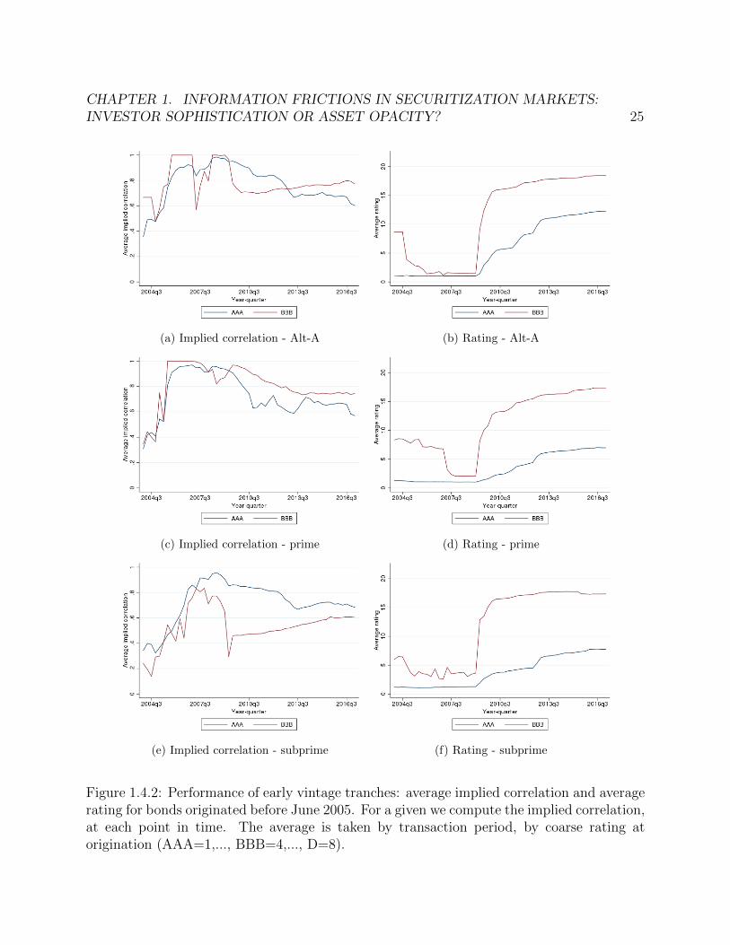
CHAPTER 1. INFORMATION FRICTIONS IN SECURITIZATION MARKETS:INVESTOR SOPHISTICATION OR ASSET OPACITY? 25
(a) Implied correlation - Alt-A (b) Rating - Alt-A
(c) Implied correlation - prime (d) Rating - prime
(e) Implied correlation - subprime (f) Rating - subprime
Figure 1.4.2: Performance of early vintage tranches: average implied correlation and averagerating for bonds originated before June 2005. For a given we compute the implied correlation,at each point in time. The average is taken by transaction period, by coarse rating atorigination (AAA=1,..., BBB=4,..., D=8).

CHAPTER 1. INFORMATION FRICTIONS IN SECURITIZATION MARKETS:INVESTOR SOPHISTICATION OR ASSET OPACITY? 26
is the dependent variable. More specifically we write
downgradei,2009 = f(α + βρi0 + ηratingi0 + γXi0 + εi). (1.12)
The independent variable of interest is the implied correlation at first transaction ρi0. Highcorrelations are detrimental to senior bondholders but beneficial to subordinate ones (Duffieand Garleanu, 2001). In line with this we expect that (except for bonds with zero subordina-tion percentage, which we do not often observe) a higher implied correlation should predicta more likely downgrade. We control for rating at origination using dummy indicators andfor vintage year. Also we cluster standard errors in all tests at the deal level, to control forthe fact that several classes in the same deal are often (down)graded at the same time.
The results in Table 1.4 replicate the findings by Ashcraft et al., 2011 that, thoughstatistically significant, ratings at origination are not sufficient for implied correlations (intheir case, coupon premium) in predicting subsequent bond downgrades. Their proxy for thebond price is the coupon premium to treasury, the hypothesis being that higher premium isreflective of more risk and thus of more downgrades. Our implied correlation measure givesa similar result. We find a positive, significant coefficient, so that higher implied correlationincreases the likelihood of downgrades. Table 1.4 breaks down this result between bondsinitially rated AAA and the rest. While the coefficient for correlation at first transactionremains significant for grades below AAA, implied correlations seem to have no predictivepower in terms of bond downgrades, similar to the findings in Adelino, 2009.
We use our opacity index to break down the sample by increments of 0.25, and presentthe results in Table 1.5. We find a ranking along the index similar to the one discussed inSection 2.4, whereby the coefficient on implied correlations is monotonically increasing inthe value of the opacity index, from insignificant at 10% for tranches below 0.25 to positiveand significant at 1% for tranches above 0.75.
Breaking down the results between AAA tranches and others shows a similar pattern.Moreover, for tranches where the documentation index is above 0.5 we have that implied cor-relation is predictive of bond downgrades. Seen together, the results suggest that uninformedinvestors are not so much those in AAA tranches as those subject to poorly documentedloans.
As a robustness check, we run the same set of regressions as before, using the deal levelaverage correlation (clustering errors at deal level) instead of the tranche implied correlation.We control for initial prices, coupons and subordinations. The results, shown in Table 1..15,suggest that correlation loses its predictive power when averaged across the deal. The av-erage at rating level, instead, retains some predictive power about subsequent downgrades.Breaking the results down by opacity index in Table 1..16, we find the same monotonicityin predictiveness of implied correlations, though the coefficient becomes significant only forthe highest values of the documentation index. However, once we break down the resultsbetween AAA and sub-AAA tranches in Table 1..17, only AAA tranche implied correlationsare predictive (still, only in the highest documentation index values). In all these tables, themonotonicity property observed before is best represented by the subordination percentage.

CHAPTER 1. INFORMATION FRICTIONS IN SECURITIZATION MARKETS:INVESTOR SOPHISTICATION OR ASSET OPACITY? 27
downgrade(1) (2) (3)All AAA only Non-AAA only
Correlation at first transaction 0.414∗∗∗ 0.299 0.268∗∗∗
(0.0629) (0.201) (0.0644)Model-implied PD 2.294∗∗ 4.308 1.503
(0.922) (3.648) (1.023)
Observations 28,991 16,618 12,371Rating at first transaction Y N YVintage year Y Y YAsset type Y Y Y
Standard errors in parentheses∗ p < 0.1, ∗∗ p < 0.05, ∗∗∗ p < 0.01
Table 1.4: Regression results from running logit regression 1.12 by maximum likelihood,controlling for vintage year (vintages up to June 2005) and model-implied probability ofdefault, as estimated in subsection 1.3. The dependent variable is a dummy indicator forwhether there was a downgrade by December 2009. Independent variables include correlationand coarse rating dummy indicator at the time of the first transaction. The dependentvariable is the downgrade indicator. Column (1) includes all issues; columns (2) and (3)split the sample between bonds rated AAA at origination and the rest, respectively. Errorsare clustered at deal level.
Low-doc assets should in principle require a form of compensation: all else constant, asophisticated investor requires more subordination when the underlying assets are opaque.Instead, Skreta and Veldkamp, 2009 predict that rating inflation is worse when assessingthe true value of the asset is difficult (making ratings noisier and more varied). For theirresult to hold, investors must be unable to infer the rating selection bias. Similarly in ourcase, investors who are unaware of the deficiency in documentation are more likely to besubjected to inflated ratings. Table 1..18 provides evidence that AAA share at originationis decreasing in our opacity index (controlling for the model-implied probability of default).This suggests that unsophisticated investors select into low-doc deals, where rating inflationis more likely to occur.
1.6 Conclusion
Two key frictions take place in securitization markets between the investor and the secu-ritizer. Though there is a role for a proxy of investor unsophistication, namely whetherthe bond is AAA-rated at origination, there is an important role of asset opacity, which wecapture using a deal-level index of documentation completeness. We observe less of a dif-

CHAPTER 1. INFORMATION FRICTIONS IN SECURITIZATION MARKETS:INVESTOR SOPHISTICATION OR ASSET OPACITY? 28
(1) (2) (3) (4)[0, 0.25) [0.25, 0.5) [0.5, 0.75) [0.75, 1]
Downgrade indicator
Correlation at first transaction 0.243 0.605∗∗∗ 0.476∗∗∗ 0.569∗∗∗
(0.250) (0.200) (0.102) (0.135)Model-implied PD 0.381 13.60 4.331 4.225∗
(1.675) (10.51) (3.000) (2.521)
Observations 2,723 6,285 7,808 5,565Rating at first transaction Y Y Y YVintage year Y Y Y YAsset type Y Y Y Y
Standard errors in parentheses∗ p < 0.10, ∗∗ p < 0.05, ∗∗∗ p < 0.01
Table 1.5: Regression results from running logit specification 1.12 by maximum likelihood,controlling for vintage year (vintages up to June 2005) and model-implied probability ofdefault as estimated in subsection 1.3. The dependent variable is a dummy indicator forwhether there was a downgrade by December 2009. Independent variables include impliedcorrelation and coarse rating dummy indicator at the time of the first transaction. Thedependent variable is the downgrade indicator. Each column presents the results on a subsetof the data corresponding to the value of the documentation index corresponding to thegiven deal. Errors are clustered at deal level.
ferential in information content across seniorities than across low-doc assets and “full-doc”ones. We show that the latter exhibit better information content across the rating spectrum.In particular, AAA implied correlations are no less predictive than the rest when the bondcomes from a deal with a high standard of documentation.
We link the information content of bond trades to the opacity on the underlying collateral,saying that more opaque loans convey less market information. The results suggest thatunsophisticated transactions select into low-doc deals. In line with this, we provide evidencethat more opaque deals tend to issue a higher proportion of AAA bonds, controlling for riskattributes of the deal. The results are consistent with ratings inflation.
Implied correlations are large in subprime deals compared to other asset classes, whichreflects a design feature of subprime loans that made them jointly dependent on houseprices. We capture this within a systematic factor framework. However, investors could beunderestimating aspects of default clustering different from systematic risk. Following Griffinand Nickerson, 2016, who argue rating agencies underestimate frailty risk, the question ofwhether contagion risk (see Appendix 1.6) is priced remains open.

CHAPTER 1. INFORMATION FRICTIONS IN SECURITIZATION MARKETS:INVESTOR SOPHISTICATION OR ASSET OPACITY? 29
(1) (2) (3) (4)
[0, 0.25) [0.25, 0.5) [0.5, 0.75) [0.75, 1]Downgrade indicator - AAA only
Correlation at first transaction 1.018 0.430 1.647∗∗∗ 0.842∗∗∗
(0.703) (0.599) (0.627) (0.321)Model-implied PD 47.95 -13.93 12.91∗∗∗ 3.301
(48.60) (45.34) (4.648) (2.970)Observations 1,529 3,765 3,975 3,429Rating at first transaction N N N NVintage year Y Y Y YAsset type Y Y Y Y
Downgrade indicator - not AAA
Correlation at first transaction 0.0485 0.370∗∗ 0.314∗∗∗ 0.353∗∗
(0.283) (0.155) (0.109) (0.158)Model-implied PD -2.323 26.14∗∗ 1.906 5.083
(2.661) (10.85) (2.607) (3.180)Observations 1,045 2,289 3,787 2,124Rating at first transaction Y Y Y YVintage year Y Y Y YAsset type Y Y Y Y
Standard errors in parentheses∗ p < 0.10, ∗∗ p < 0.05, ∗∗∗ p < 0.01
Table 1.6: Regression results from running logit specification 1.12 by maximum likelihood,controlling for vintage year (vintages up to June 2005) and model-implied probability ofdefault as estimated in subsection 1.3. The dependent variable is a dummy indicator forwhether there was a downgrade by December 2009. Independent variables include impliedcorrelation and coarse rating dummy indicator at the time of the first transaction. Thedependent variable is the downgrade indicator. Each column presents the results on a subsetof the data corresponding to the value of the documentation index corresponding to thegiven deal. Errors are clustered at deal level.

30
Appendix

CHAPTER 1. INFORMATION FRICTIONS IN SECURITIZATION MARKETS:INVESTOR SOPHISTICATION OR ASSET OPACITY? 31
Supplemental graphs and tables
Asset typeAfter Jun-05 Before Jun-05
Origination ($bn) Count Origination ($bn) CountAlt-A 1,179.0 16,837 557.7 11,000Prime 621.7 9,097 557.9 14,759Second Lien 64.7 478 19.0 408Subprime 660.0 9,811 720.2 9,525Total 2,525.4 36,223 1,854.8 35,692
Table 1..7: Issued amounts and counts by asset type.
(a) Number of tranches (b) Total issue
Figure 1..1: Number of tranches and amount issued by vintage year for private label collat-eralized mortgage obligations. Source: ABSNet bond data. For our sample of early vintages(prior to June 2005) we provide the distribution by (coarse, see Table 1..20) initial rating.
Data cleaning
Bond data
We start with 16,397,826 panel observations, corresponding to 127,963 tranches. I removedata entry errors such as subordination percentages larger than one. In those cases allobservations for the month (all tranches linked to the deal involved) are removed so as toensure computations of the tranching structure are correct.21 We follow Adelino, 2009 in
21I manually computed subordination percentages on a random sample of deals to check the calculationsby ABSNet.

CHAPTER 1. INFORMATION FRICTIONS IN SECURITIZATION MARKETS:INVESTOR SOPHISTICATION OR ASSET OPACITY? 32
Our sample Cordell, Huang, and Williams, 2012rating Prime/Alt-A Second Lien/Subprime Prime/Alt-A Second Lien/SubprimeAAA 10.8% 25.7% 6% 23%AA 3.4% 14.3% 3% 13%A 3.0% 5.9% 2% 8%BBB 2.9% 4.0% 1% 4%
Table 1..8: Subordination percentage by tranche rating - comparison. The figures computedusing ABSNet data are derived by aggregating the subordination percentages at orginationas given in Table 1.2.4. Our sample contains only early vintages (prior to June 2005) whileCordell, Huang, and Williams, 2012 use late vintages as well.
YearABSNet sample Adelino, 2009
Origination ($bn) Count Origination ($bn) Count≤2002 319.3 5,438
2003 470.5 10,120 496.5 8,5742004 677.4 12,519 767.3 11,4602005 904.5 16,684 1,058.5 17,1352006 1,038.0 15,022 1,080.4 18,2062007 939.4 11,716 802.1 12,037≥2008 31.2 177Total 4,380.3 71,676 4,204.8 67,412
Table 1..9: Origination amounts and counts at origination, by vintage year, compared to thesample in Adelino, 2009.
(1) (2)
Asset type Early vintages Late vintages
Alt-A 7.5% 19.5%
Prime 2.3% 6.6%
Second Lien 7.2% 25.8%
Subprime 14.8% 30.5%
Observations 4,060,698 631,793
Table 1..10: Liquidation rates from the loan sample. Column (1) calculates the percentageof loans linked to early vintage deals (before June 2005) that are liquidated. Column (2)calculates the same ratio for late vintage loans.
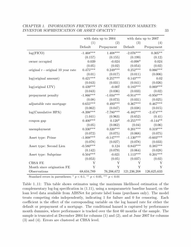
CHAPTER 1. INFORMATION FRICTIONS IN SECURITIZATION MARKETS:INVESTOR SOPHISTICATION OR ASSET OPACITY? 33
with data up to 2004 with data up to 2007(1) (2) (3) (4)
Default Prepayment Default Prepayment
log(FICO) -1.468*** 1.408*** -2.076*** 0.305**(0.157) (0.155) (0.199) (0.12)
owner occupied 0.039 -0.024 -0.098* 0.024(0.05) (0.02) (0.054) (0.02)
original r - original 10 year rate 0.475*** 0.249*** 0.252*** 0.066***(0.01) (0.017) (0.011) (0.006)
log(original amount) 0.421*** 0.257*** 0.143*** 0.02(0.043) (0.031) (0.041) (0.026)
log(original LTV) 0.439*** -0.007 0.183*** 0.069***(0.043) (0.036) (0.033) (0.02)
prepayment penalty -1.866*** -1.034*** -0.914*** -0.950***(0.08) (0.073) (0.031) (0.025)
adjustable rate mortgage 0.655*** 0.493*** 0.367*** 0.467***(0.062) (0.047) (0.038) (0.015)
log(Cumulative HPA) -8.398*** -7.780*** -6.482*** -2.474***(1.041) (0.963) (0.652) (0.41)
coupon gap 0.400*** 0.120* -0.255*** -0.144**(0.05) (0.062) (0.04) (0.06)
unemployment 0.330*** 0.320*** 0.201*** 0.319***(0.072) (0.075) (0.068) (0.075)
Asset type: Prime -1.008*** -0.147*** -1.130*** -0.603***(0.078) (0.027) (0.078) (0.033)
Asset type: Second Lien -0.580*** 0.124 0.843*** 0.385***(0.142) (0.079) (0.064) (0.028)
Asset type: Subprime 0.504*** -0.021 1.113*** 0.201***(0.053) (0.05) (0.037) (0.02)
CBSA FE Y Y Y YMonth since origination FE Y Y Y YObservations 68,634,789 76,206,672 121,236,208 126,625,633
Standard errors in parentheses; ∗ p < 0.1, ∗∗ p < 0.05, ∗∗∗ p < 0.01
Table 1..11: This table shows estimates using the maximum likelihood estimation of thecomplementary log-log specification in (1.11), using a nonparametric baseline hazard, on theloan level data available from ABSNet for private label loans (purchases only). The modeltreats competing risks independently, indicating 1 for failure and 0 for censoring. Eachcoefficient is the effect of the corresponding variable on the log hazard rate for either thedefault or prepayment of a mortgage. The conditional hazard is captured by performancemonth dummies, where performance is tracked over the first 60 months of the sample. Thesample is truncated at December 2004 for columns (1) and (2), and at June 2007 for columns(3) and (4). Errors are clustered at CBSA level.

CHAPTER 1. INFORMATION FRICTIONS IN SECURITIZATION MARKETS:INVESTOR SOPHISTICATION OR ASSET OPACITY? 34
(1) (2)default prepayment
log(FICO) -2.481*** 0.448***(0.064) (0.018)
owner occupied 0.025* 0.372***(0.014) (0.005)
original r - original 10 year rate 0.429*** -0.011***(0.004) (0.001)
log(original amount) 0.137*** 0.324***(0.01) (0.003)
log(original LTV) 0.572*** 0.183***(0.012) (0.005)
adjustable rate mortgage 0.487*** 0.579***(0.016) (0.004)
log(Cumulative HPA) -1.826*** -1.581***(0.051) (0.011)
coupon gap 0.848*** -0.261***(0.007) (0.002)
unemployment 0.080*** 0.001(0.004) (0.001)
Asset type: Prime -0.808*** -2.719***(0.044) (0.014)
Asset type: Second Lien -0.794*** 0.298***(0.038) (0.011)
Asset type: Subprime 0.402*** 1.079***(0.025) (0.005)
CBSA FE N NMonth since origination FE N YObservations 2,630,290 76,374,400
Standard errors in parentheses; ∗ p < 0.1, ∗∗ p < 0.05, ∗∗∗ p < 0.01
Table 1..12: This table shows estimates using the maximum likelihood estimation of a com-plementary log-log specification, using a hazard specification for prepayments and a dummyindicator for default, on the loan level data available from ABSNet for private label loans(purchases only). The hazard model treats default risk as censored. Each coefficient is theeffect of the corresponding variable on the log hazard rate for prepayment or the log prob-ability of default of a mortgage. The conditional hazard is captured by performance monthdummies, where performance is tracked over the first 60 months of the sample. The sampleis truncated at December 2004.

CHAPTER 1. INFORMATION FRICTIONS IN SECURITIZATION MARKETS:INVESTOR SOPHISTICATION OR ASSET OPACITY? 35
default
indicator(bytheen
dofthegiven
year)
2000
2001
2002
2003
2004
2005
2006
2007
2008
2009
log(F
ICO)
-2.485***
-3.599***
-4.816***
-2.583***
-3.141***
-3.682***
-4.561***
-4.160***
-3.029***
-2.059***
(0.494)
(0.257)
(0.151)
(0.101)
(0.071)
(0.052)
(0.038)
(0.027)
(0.018)
(0.014)
owner
occupied
-0.318**
0.037
0.263***
0.133***
-0.214***
-0.329***
-0.333***
-0.247***
-0.097***
-0.148***
(0.139)
(0.069)
(0.041)
(0.024)
(0.016)
(0.011)
(0.008)
(0.006)
(0.004)
(0.003)
originalr-original
-0.052
0.277***
0.199***
0.431***
0.459***
0.343***
0.164***
0.178***
0.158***
0.102***
10yearrate
(0.038)
(0.018)
(0.011)
(0.006)
(0.004)
(0.003)
(0.002)
(0.001)
(0.001)
(0.001)
log(originalamount)
-0.053
-0.038
-0.235***
0.125***
0.150***
-0.026***
-0.297***
-0.126***
-0.029***
-0.013***
(0.084)
(0.043)
(0.025)
(0.016)
(0.011)
(0.007)
(0.005)
(0.003)
(0.002)
(0.002)
log(originalLTV)
0.828***
0.698***
0.585***
0.772***
0.682***
0.548***
0.445***
0.178***
0.124***
0.078***
(0.266)
(0.099)
(0.030)
(0.019)
(0.014)
(0.010)
(0.007)
(0.004)
(0.003)
(0.002)
adjustable
rate
-0.707***
0.145**
0.305***
0.335***
0.261***
0.269***
0.291***
-0.045***
-0.130***
0.001
mortgage
(0.104)
(0.058)
(0.035)
(0.023)
(0.016)
(0.011)
(0.008)
(0.006)
(0.004)
(0.003)
log(cumulativeHPA)
1.921***
2.981***
4.548***
-3.303***
-1.878***
-0.877***
0.412***
-1.998***
-5.796***
-4.319***
(0.676)
(0.248)
(0.122)
(0.103)
(0.054)
(0.030)
(0.018)
(0.017)
(0.011)
(0.007)
coupongap
-1.930***
0.216***
-0.591***
1.234***
0.998***
0.832***
0.170***
-1.057***
-0.810***
0.889***
(0.062)
(0.037)
(0.019)
(0.013)
(0.009)
(0.006)
(0.005)
(0.004)
(0.002)
(0.002)
unem
ploymen
t0.137***
-1.052***
-0.342***
-0.080***
0.011**
0.126***
0.176***
0.004***
-0.183***
-0.309***
(0.037)
(0.026)
(0.014)
(0.009)
(0.006)
(0.003)
(0.002)
(0.002)
(0.001)
(0.001)
Asset
type:
Prime
0.000
-1.048***
-0.805***
-0.748***
-0.621***
-0.299***
-0.248***
-0.669***
-1.456***
-1.640***
(.)
(0.245)
(0.100)
(0.068)
(0.049)
(0.035)
(0.028)
(0.024)
(0.018)
(0.011)
Asset
type:
SecondLien
0.000
-3.509***
-5.936***
-4.410***
-1.984***
-0.213***
0.471***
0.877***
0.639***
0.616***
(.)
(1.012)
(1.002)
(0.271)
(0.062)
(0.027)
(0.018)
(0.012)
(0.007)
(0.005)
Asset
type:
Subprime
2.872***
0.939***
0.213***
0.147***
0.274***
0.438***
0.742***
1.027***
0.777***
0.710***
(0.311)
(0.128)
(0.062)
(0.040)
(0.028)
(0.019)
(0.014)
(0.010)
(0.005)
(0.004)
Obs
230,631
516,866
865,545
1,435,035
2,630,290
4,307,739
5,766,680
6,014,866
6,014,866
6,014,866
Sta
nd
ard
erro
rsin
par
enth
eses
∗p<
0.1
,∗∗p<
0.0
5,∗∗∗p<
0.01
Tab
le1.
.13:
This
table
show
ses
tim
ates
usi
ng
the
max
imum
like
lihood
esti
mat
ion
ofa
com
ple
men
tary
log-
log
spec
-ifi
cati
on,
usi
ng
adum
my
indic
ator
for
def
ault
,on
the
loan
leve
ldat
aav
aila
ble
from
AB
SN
etfo
rpri
vate
lab
ello
ans
(purc
has
eson
ly).
For
each
year
,va
riab
les
are
take
nat
the
mea
sure
men
tp
oint
(eit
her
def
ault
tim
e,if
def
ault
ed,
orob
serv
atio
nti
me,
whic
his
the
end
ofth
egi
ven
year
).
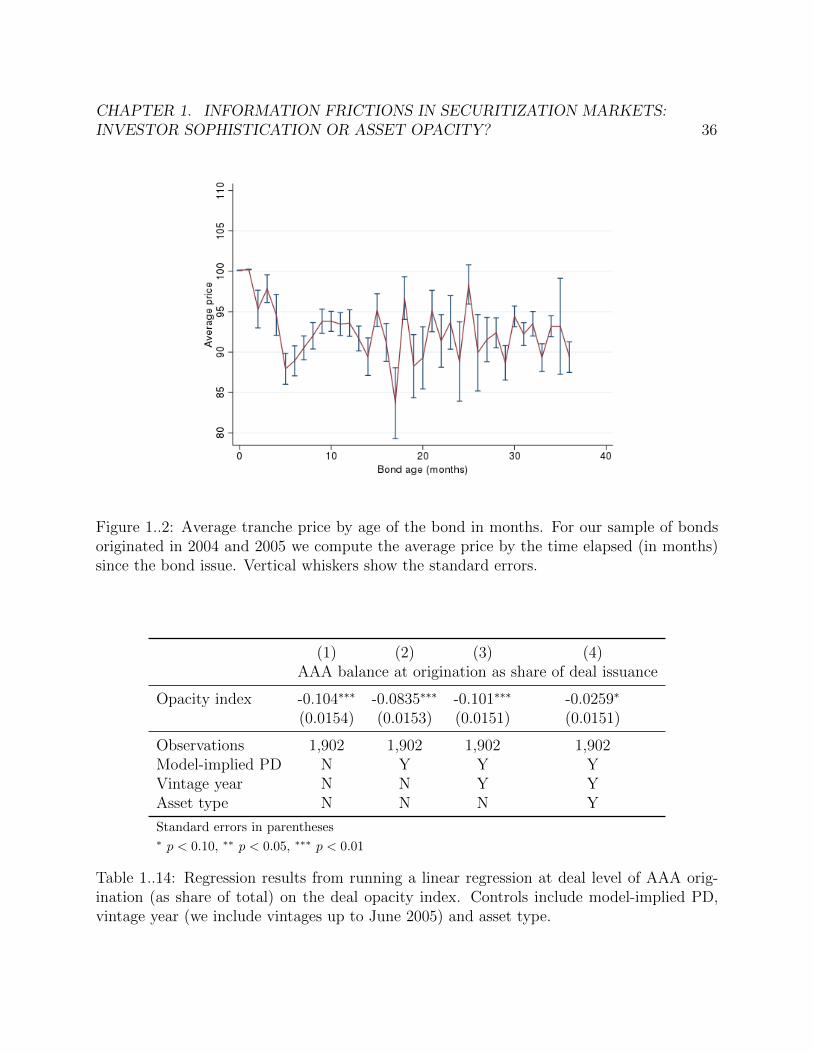
CHAPTER 1. INFORMATION FRICTIONS IN SECURITIZATION MARKETS:INVESTOR SOPHISTICATION OR ASSET OPACITY? 36
Figure 1..2: Average tranche price by age of the bond in months. For our sample of bondsoriginated in 2004 and 2005 we compute the average price by the time elapsed (in months)since the bond issue. Vertical whiskers show the standard errors.
(1) (2) (3) (4)AAA balance at origination as share of deal issuance
Opacity index -0.104∗∗∗ -0.0835∗∗∗ -0.101∗∗∗ -0.0259∗
(0.0154) (0.0153) (0.0151) (0.0151)
Observations 1,902 1,902 1,902 1,902Model-implied PD N Y Y YVintage year N N Y YAsset type N N N Y
Standard errors in parentheses∗ p < 0.10, ∗∗ p < 0.05, ∗∗∗ p < 0.01
Table 1..14: Regression results from running a linear regression at deal level of AAA orig-ination (as share of total) on the deal opacity index. Controls include model-implied PD,vintage year (we include vintages up to June 2005) and asset type.

CHAPTER 1. INFORMATION FRICTIONS IN SECURITIZATION MARKETS:INVESTOR SOPHISTICATION OR ASSET OPACITY? 37
downgrade(1) (2) (3)All AAA only Non-AAA only
Deal average correlation 0.211(0.189)
Average correlation within rating bucket 0.721∗ 0.369∗
(0.427) (0.217)Price -0.0185∗∗∗ -0.0446∗∗∗ -0.00937∗∗∗
(0.00152) (0.00305) (0.00150)Coupon -0.123∗∗∗ -0.0402 -0.183∗∗∗
(0.0178) (0.0245) (0.0240)Subordination -3.168∗∗∗ -4.144∗∗∗ -4.113∗∗∗
(0.271) (0.601) (0.316)
Observations 26,242 14,034 12,206Rating at first transaction Y N YVintage year Y Y YAsset type Y Y Y
Standard errors in parentheses∗ p < 0.1, ∗∗ p < 0.05, ∗∗∗ p < 0.01
Table 1..15: Regression results from running logit regression 1.12 by maximum likelihood,controlling for vintage year (vintages up to June 2005) and model-implied probability ofdefault, as estimated in subsection 1.3. The dependent variable is a dummy indicator forwhether there was a downgrade by December 2009. Column (1) includes all issues; columns(2) and (3) split the sample between bonds rated AAA at origination and the rest, respec-tively. Independent variables include deal level average correlation (column 1), AAA averagecorrelation (column 2), sub-AAA average correlation (column 3) and coarse rating dummyindicator at the time of the first transaction. The dependent variable is the downgradeindicator. Errors are clustered at deal level.

CHAPTER 1. INFORMATION FRICTIONS IN SECURITIZATION MARKETS:INVESTOR SOPHISTICATION OR ASSET OPACITY? 38
Figure 1..3: Average subordination difference between AAA and BBB bonds. Source: AB-SNet bond data.The figure presents the difference between the average AAA and averageBBB subordination over trading time (for early vintages, prior to June 2005) using the ratingat the given trading time. The difference is computed by asset type.
removing Interest Only, Principal Only, Inverse Floater and Fixed to Variable bonds fromthe sample.
Notice that the most aggressive cleaning step is the removal of observations where priceis missing. As dicussed in subsection 1.2, this is due to the data gap that covers late (2005and more recent) vintages.
Loan level data
We start with a set of 22,008,610 loan originations. Of our originations set, 21,759,836 mapto one of our deal IDs. Below is a summary of deal level averages of certain covariates (FICOscore, LTV, private mortgage insurance coverage percentage) are computed.22
Historic data are contained in monthly reports. From the input 21,996,382 facilities wehave at least one observation for 17,350,072 of them. We recover a total 792,664,139 loan-month observations from payment history (on average 45.7 obs per loan). From there wecan compute default rates at deal level. We have loss event data for 3,986,974 observations,linked to 5,965 deal IDs. From there we can compute LGDs at deal level or vintage level.
22Simple averages were preferred over weighted averages (weighted by e.g. the initial securitized balance)as this reduces the number of missing observations.

CHAPTER 1. INFORMATION FRICTIONS IN SECURITIZATION MARKETS:INVESTOR SOPHISTICATION OR ASSET OPACITY? 39
Figure 1..4: Probability of default by vintage year. We compute the default rate for eachof the deals that compose our population, and then average by vintage year and asset type.The results are presented here along with standard error bands around the average.
At the loan level, we keep only loans having purchase as purpose. This reduces the sampleto 8,862,561 loans. Aside minor cleaning (originations before 1980, errors in time stamps)we arrive to 7,145,251. From these we discard asset types other than Alt-A, Prime, SecondLien or Subprime to arrive at the initial sample composed of early and late vintages.
Variations on the baseline model
Pricing results with constant default probability and prepayment speed
In this section we use a constant PD, by asset type, given as theAfter the collapse of private label securitization in 2007, most securitization conduits are
insured against default risk by the Government-Sponsored Entities (Fannie Mae and Fred-die Mac), making prepayment risk the most significant one in the literature. Schwartz andTorous, 1989 and Stanton, 1995 measure the value of prepayment option in default-free secu-rities (guaranteed by the Government-Sponsored Entities). Downing, Stanton, and Wallace,2005 propose a two-factor valuation model that distinguishes the separate, competing riskscarried by the default and the prepayment options. Sugimura, 2004 develops an intensitymodel to price RMBS (pass-through) bonds not insured against default risk, and thus ex-posed to both prepayment and default risk (but credit events in his approach are assumed

CHAPTER 1. INFORMATION FRICTIONS IN SECURITIZATION MARKETS:INVESTOR SOPHISTICATION OR ASSET OPACITY? 40
Figure 1..5: Percentage loss given default by vintage year. The aggregate loss given defaultis computed from the sample of loans associated to the deals that compose our populationof CMOs.
to be uncorrelated). We seek an accurate measure of prepayment while keeping the focus ondefault risk, hence the choice of the PSA schedule (see Figure 1..7).
In order to chose the PSA factor we look at the class balance. Class balance factor, whichmeasures balance over time relative to the tranche initial balance, reflects both losses andprepayments, thus is an upper bound for prepayments. The results in Figure 1..6 suggest that150% is an appropriate upper bound. Gorton, 2009 states that subprime deals were mostlylinked to ARMs (see Figure 1..10), those being a priori subject to higher prepayment rates.23
The evolution of class factor over time does not suggest a radically different prepayment ratefor subprime deals in our sample. In this section we will apply the PSA schedule, with afactor of 150%, to all tranches within the same deal.
Cornaggia, Cornaggia, and Hund, 2017 find that ratings are not comparable across broadasset types (corporate, CDO, ABS and RMBS). Within RMBS we emphasize the differenceacross asset types (prime, subprime and Alt-A), and in this section document a differencein information across asset types, namely between Alt-A and other types.
Breaking the change by asset type we see an increase for Alt-A tranches (from 0.36 to0.40), no change for prime ones (0.30) and a decrease for subprime deals (from 0.59 to 0.49,
23He finds that the shift to subprime deals happened for the later cohorts. Similarly, we find that latercohorts see faster reductions in balance.

CHAPTER 1. INFORMATION FRICTIONS IN SECURITIZATION MARKETS:INVESTOR SOPHISTICATION OR ASSET OPACITY? 41
Figure 1..6: Average class balance factor by asset class over tranche age. Alongside theaverages, we compute the balance factor that results from a 150% payment schedule alone(excluding planned amortization).
Figure 1..7: Standard Prepayment Model of The Bond Market Association. Prepaymentpercentage for each month in the life of the underlying mortgages, expressed on an annualizedbasis.

CHAPTER 1. INFORMATION FRICTIONS IN SECURITIZATION MARKETS:INVESTOR SOPHISTICATION OR ASSET OPACITY? 42
Figure 1..8: Plot of average class factor against tranche age by tranche initial rating.
significant at 99%) so that the upward adjustment during seems to have mainly affectedAlt-A issues.
In terms of seniorities, the difference observed by Buzkova and Teply, 2012 over the crisisis mainly driven by mezzanine tranches (7%-10% and 10%-15%). Figure 1..17 also suggeststhe increase in correlations is larger among intermediate seniorities, though not as large asthe one they observe on the CDX tranches.
The regression results on price informativeness are similar to those obtained in Section 1.4:implied default correlations are informative when they are linked to well-documented deals,which happens both for AAA and non-AAA tranches. First, the results in Table 1..22 confirmthose of Table 1.4 in that implied correlations are informative about bond downgrades, exceptfor AAA tranches. Second, the split by opacity index (see Table 1..24) yields a similar resultsto that in Table 1.5. Finally, the further split by rating in Table 1..24 yields results that areconsistent with those in Table 1.5.
The information content of news in prices
Using the partial observations we recover from the ABSNet data (namely, observations postJune 2009) we study the effect of news in prices across the cycle. A number of cleaningstages (see Table 1..19 in the appendix) are applied to attain the final sample, which contains
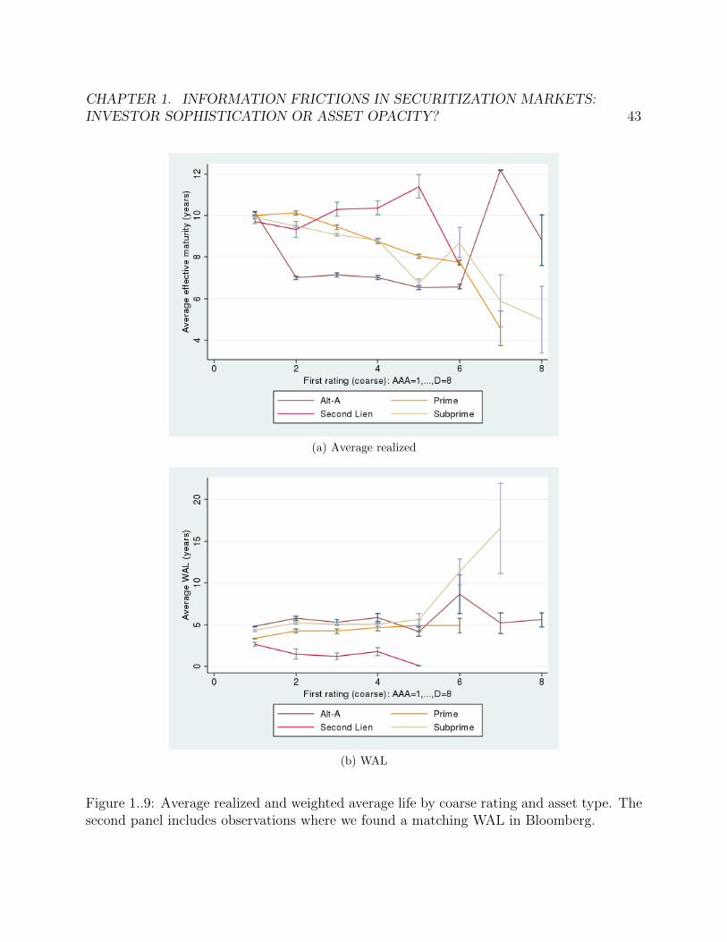
CHAPTER 1. INFORMATION FRICTIONS IN SECURITIZATION MARKETS:INVESTOR SOPHISTICATION OR ASSET OPACITY? 43
(a) Average realized
(b) WAL
Figure 1..9: Average realized and weighted average life by coarse rating and asset type. Thesecond panel includes observations where we found a matching WAL in Bloomberg.

CHAPTER 1. INFORMATION FRICTIONS IN SECURITIZATION MARKETS:INVESTOR SOPHISTICATION OR ASSET OPACITY? 44
Figure 1..10: Proportion of ARM loans by vintage and asset type.
Figure 1..11: Number of deals originated by asset type and vintage year.

CHAPTER 1. INFORMATION FRICTIONS IN SECURITIZATION MARKETS:INVESTOR SOPHISTICATION OR ASSET OPACITY? 45
Figure 1..12: Histogram plotting all outcomes from the pricing model.
6,322,690 panel observations -close to 64 transactions per tranche-. We illustrate the overallnumbers in Figure 1..18.
The results up to now suggest implied correlation at origination is predictive of down-grades to the extent that the loans have full documentation. Having seen the role of initialsignals, our next question is about the role of price news both from rating agencies and themarket. While initial ratings rely on an a priori assessment, its evolution over time reflectsprogressively more of the bond performance, implying that updated rating values should inprinciple absorb the information that was initially private. We estimate panel 1.13 usinga linear model, with random effects in order to control for tranche-invariants such as firstrating and first implied correlation. The advantage of the panel specification 1.13 is that wecan incorporate the partial information coming from the late vintages (after June 2005).
outcomeit = αit + β0ρi,0 + η0ratingi0 + β1ρi,t−1 + η1ratingi,t−1 + γXi,t + εit. (1.13)
In equation 1.13 outcomeit is the month-on-month rating change in notches. Table 1..26shows that updates in signals contain information about future bond performance, but thesignal is not statistically sufficient for prices. This suggests that investors retain privateinformation over the life of the bond, besides the information given by agency ratings. Thesecond finding is that Alt-A investors do not learn over the life of the bond, so that news inratings remain statistically sufficient for news in correlation in terms of bond performance.
To see the effect of the crisis on the information content of prices, we will use interactionswith an indicator dummy for post-2007 transaction to split estimates between before and
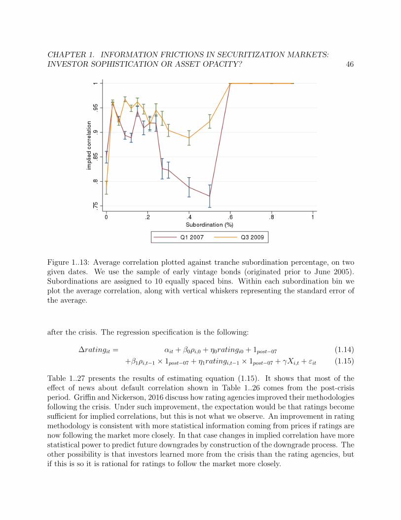
CHAPTER 1. INFORMATION FRICTIONS IN SECURITIZATION MARKETS:INVESTOR SOPHISTICATION OR ASSET OPACITY? 46
Figure 1..13: Average correlation plotted against tranche subordination percentage, on twogiven dates. We use the sample of early vintage bonds (originated prior to June 2005).Subordinations are assigned to 10 equally spaced bins. Within each subordination bin weplot the average correlation, along with vertical whiskers representing the standard error ofthe average.
after the crisis. The regression specification is the following:
∆ratingit = αit + β0ρi,0 + η0ratingi0 + 1post−07 (1.14)
+β1ρi,t−1 × 1post−07 + η1ratingi,t−1 × 1post−07 + γXi,t + εit (1.15)
Table 1..27 presents the results of estimating equation (1.15). It shows that most of theeffect of news about default correlation shown in Table 1..26 comes from the post-crisisperiod. Griffin and Nickerson, 2016 discuss how rating agencies improved their methodologiesfollowing the crisis. Under such improvement, the expectation would be that ratings becomesufficient for implied correlations, but this is not what we observe. An improvement in ratingmethodology is consistent with more statistical information coming from prices if ratings arenow following the market more closely. In that case changes in implied correlation have morestatistical power to predict future downgrades by construction of the downgrade process. Theother possibility is that investors learned more from the crisis than the rating agencies, butif this is so it is rational for ratings to follow the market more closely.

CHAPTER 1. INFORMATION FRICTIONS IN SECURITIZATION MARKETS:INVESTOR SOPHISTICATION OR ASSET OPACITY? 47
(a) Alt-A (b) Prime
(c) Subprime
Figure 1..14: Average correlation plotted against tranche subordination percentage, on twogiven dates. Subordination values are assigned to 10 equally spaced bins. Within eachsubordination bin we plot the average correlation, along with vertical whiskers representingthe standard error of the average.
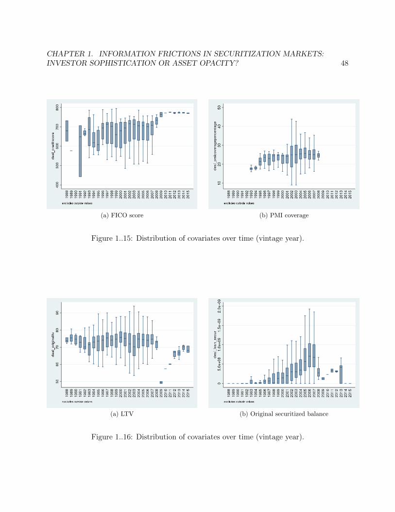
CHAPTER 1. INFORMATION FRICTIONS IN SECURITIZATION MARKETS:INVESTOR SOPHISTICATION OR ASSET OPACITY? 48
(a) FICO score (b) PMI coverage
Figure 1..15: Distribution of covariates over time (vintage year).
(a) LTV (b) Original securitized balance
Figure 1..16: Distribution of covariates over time (vintage year).

CHAPTER 1. INFORMATION FRICTIONS IN SECURITIZATION MARKETS:INVESTOR SOPHISTICATION OR ASSET OPACITY? 49
(1) (2) (3) (4)[0, 0.25) [0.25, 0.5) [0.5, 0.75) [0.75, 1]
Downgrade indicator
Deal average correlation -0.581 -0.155 -0.0162 0.901∗∗
(0.750) (0.522) (0.367) (0.395)Price -0.0165∗∗∗ -0.0202∗∗∗ -0.0110∗∗∗ -0.0167∗∗∗
(0.00631) (0.00343) (0.00269) (0.00356)Coupon -0.134∗∗ -0.0369 -0.117∗∗∗ -0.0749
(0.0649) (0.0310) (0.0442) (0.0465)Subordination -0.0512 -1.869∗∗∗ -4.013∗∗∗ -5.858∗∗∗
(0.852) (0.653) (0.489) (0.959)
Observations 2,489 5,513 7,073 5,049Rating at first transaction Y Y Y YVintage year Y Y Y YAsset type Y Y Y Y
Standard errors in parentheses∗ p < 0.10, ∗∗ p < 0.05, ∗∗∗ p < 0.01
Table 1..16: Regression results from running logit specification 1.12 by maximum likelihood,controlling for vintage year (vintages up to June 2005) and model-implied probability ofdefault as estimated in subsection 1.3. The dependent variable is a dummy indicator forwhether there was a downgrade by December 2009. Independent variables include deallevel average implied correlation and coarse rating dummy indicator at the time of the firsttransaction. The dependent variable is the downgrade indicator. Each column presentsthe results on a subset of the data corresponding to the value of the documentation indexcorresponding to the given deal. Errors are clustered at deal level.
In DeMarzo, 2005, two factors drive the benefits and drawbacks of securitization: privateinformation by the issuer, on one hand, and asset correlation, on the other. Like CDOs,CMOs are a priori affected by it.24 Our measure of beliefs about default correlation reflectsin part adverse selection concerns on the part of the investors. Because we can’t disentanglethese two components empirically, our implied correlation measure is a proxy for marketconservatism vis-a-vis information asymmetry. In line with this, Alt-A deals being morereliant on ratings (not only for the first transaction, but also for subsequent ones) potentiallyreflects a concern for asymmetric information as in Adelino, Gerardi, and Hartman-Glaser,2016.
24Beltran, Cordell, and Thomas, 2017 show that, under asymmetric information, even a modest percentageof bad securities can push security prices far below fundamentals -even to a market meltdown-.

CHAPTER 1. INFORMATION FRICTIONS IN SECURITIZATION MARKETS:INVESTOR SOPHISTICATION OR ASSET OPACITY? 50
(1) (2) (3) (4)
[0, 0.25) [0.25, 0.5) [0.5, 0.75) [0.75, 1]Downgrade indicator - AAA only
AAA average correlation 5.310 0.701 1.074 3.019∗∗∗
(3.508) (1.594) (0.962) (0.857)Price -0.0309∗∗∗ -0.0351∗∗∗ -0.0328∗∗∗ -0.0535∗∗∗
(0.00991) (0.00542) (0.00655) (0.0118)Coupon 0.0452∗∗∗ 0.0544 0.0898 0.149∗∗
(0.0173) (0.0453) (0.0580) (0.0726)Subordination 0.610 -2.791∗∗ -2.283 -11.79∗∗∗
(1.530) (1.260) (1.851) (4.377)Observations 1,325 3,073 3,272 2,926Rating at first transaction N N N NVintage year Y Y Y YAsset type Y Y Y Y
Downgrade indicator - not AAA
Below-AAA average correlation -1.266 0.527 -0.0727 0.195(0.886) (0.548) (0.431) (0.574)
Price -0.0154∗∗ -0.0127∗∗∗ -0.00783∗∗∗ -0.0115∗∗∗
(0.00704) (0.00370) (0.00249) (0.00362)Coupon -0.357∗∗∗ -0.174∗∗∗ -0.201∗∗∗ -0.155∗∗∗
(0.103) (0.0496) (0.0529) (0.0599)Subordination 0.133 -2.715∗∗∗ -4.482∗∗∗ -4.278∗∗∗
(1.905) (0.878) (0.541) (0.852)Observations 1,038 2,248 3,757 2,111Rating at first transaction Y Y Y YVintage year Y Y Y YAsset type Y Y Y Y
Standard errors in parentheses∗ p < 0.10, ∗∗ p < 0.05, ∗∗∗ p < 0.01
Table 1..17: Regression results from running logit specification 1.12 by maximum likelihood,controlling for vintage year (vintages up to June 2005) and model-implied probability ofdefault as estimated in subsection 1.3. The dependent variable is a dummy indicator forwhether there was a downgrade by December 2009. Independent variables include AAAaverage correlation (upper panel), sub-AAA average correlation (lower panel) and coarserating dummy indicator at the time of the first transaction. The dependent variable is thedowngrade indicator. Each column presents the results on a subset of the data correspondingto the value of the documentation index corresponding to the given deal. Errors are clusteredat deal level.

CHAPTER 1. INFORMATION FRICTIONS IN SECURITIZATION MARKETS:INVESTOR SOPHISTICATION OR ASSET OPACITY? 51
(1) (2) (3) (4)AAA balance at origination as share of deal issuance
Opacity index -0.104∗∗∗ -0.0835∗∗∗ -0.101∗∗∗ -0.0259∗
(0.0154) (0.0153) (0.0151) (0.0151)
Observations 1,902 1,902 1,902 1,902Model-implied PD N Y Y YVintage year N N Y YAsset type N N N Y
Standard errors in parentheses∗ p < 0.10, ∗∗ p < 0.05, ∗∗∗ p < 0.01
Table 1..18: Regression results from running a linear regression at deal level of AAA orig-ination (as share of total) on the deal opacity index. Controls include model-implied PD,vintage year (we include vintages up to June 2005) and asset type.
Stage Tranches leftRemove deals that are entirely made of mixed asset types 119,215Remove deals where one tranche has subordination >1 119,215Remove observations with missing price 74,307Remove mixed-type asset pools 74,253Remove PO, IO, IF and FtV 71,950
Table 1..19: Data cleaning stages with number of tranches outstanding at the end of eachstep.
Additional causes of default clustering: frailty and contagion
Following Azizpour, Giesecke, and Schwenkler, 2016, defaults are driven by three factors:systemic risk25 as captured by macroeconomic variables (Bullard, Neely, and Wheelock,2009; Khandani, Lo, and Merton, 2013)26, an unobserved frailty factor (Duffie et al., 2009;
25Bisias et al. (2012) provides a survey of systemic risk measures. See also Chan-Lau et al. (2009).Other approaches include macro measures (costly asset-price boom/bust cycles, property-price, equity-price,credit-gap indicators), forward-looking measures (e.g. absorption rate as in Kritzman et al. (2010)), cross-subsectional measures (CoVaR, Co-Risk, marginal and systemic expected shortfall, see Acharya et al. (2012)),stress tests (e.g. Duffie (2011)), illiquidity and insolvency (e.g. Brunnermeier, Gorton, and Krishnamurthy(2011)). Giglio et al. (2013) use predictive quantile regression to provide an empirical assessment of 17of them. Their main finding is that, overall, the compendium of systemic risk measures contains usefulpredictive information. Instead individual measures tend to fail in capturing systematic risk.
26The characterization of systemic risk as deterioration of macroeconomic indicators leaves aside thewidely discussed view that the pre-crisis mortgage system was systemically vulnerable (Hellwig, 2009; Poitrasand Zanotti, 2016).

CHAPTER 1. INFORMATION FRICTIONS IN SECURITIZATION MARKETS:INVESTOR SOPHISTICATION OR ASSET OPACITY? 52
S&P rating Code Coarse rating CodeAAA 1 AAA 1AA+ 2 AA 2AA 3 AA 2AA- 4 AA 2A+ 5 A 3A 6 A 3A- 7 A 3BBB+ 8 BBB 4BBB 9 BBB 4BBB- 10 BBB 4BB+ 11 BB 5BB 12 BB 5BB- 13 BB 5B+ 14 B 6B 15 B 6B- 16 B 6CCC 17 C 7CCC- 18 C 7CC 19 C 7C 20 C 7D 21 D 8NR - NR -
Table 1..20: Mapping of ratings - fine and coarse level (with numbering code)
(1) (2) (3)
Asset type Early vintages Late vintages Model PD
Alt-A 7.5% 19.5% 24.5%
Prime 2.3% 6.6% 6.4%
Second Lien 7.2% 25.8% 21.1%
Subprime 14.8% 30.5% 30%
Observations 4,060,698 631,793 2,112
Table 1..21: Liquidation rates from the loan sample, and PD used for baseline estimation.Column (1) calculates the percentage of loans linked to early vintage deals (before June 2005)that are liquidated. Column (2) calculates the same ratio for late vintage loans. Column (3)shows the PD parameters used for the pricing model, calculated as the average of the deallevel liquidation rates for both early and late deals.

CHAPTER 1. INFORMATION FRICTIONS IN SECURITIZATION MARKETS:INVESTOR SOPHISTICATION OR ASSET OPACITY? 53
downgrade(1) (2) (3)All AAA only Non-AAA only
Correlation at first transaction 0.248∗∗∗ 0.0378 0.138∗∗
(0.0531) (0.114) (0.0561)
Observations 29,938 17,234 12,702Rating at first transaction Y N YVintage year Y Y Y
Standard errors in parentheses∗ p < 0.1, ∗∗ p < 0.05, ∗∗∗ p < 0.01
Table 1..22: Regression results from running logit regression 1.12 by maximum likelihood,controlling for vintage year, for vintages up to June 2005. The dependent variable is a dummyindicator for whether there was a downgrade by December 2009. Independent variables in-clude correlation and coarse rating dummy indicator at the time of the first transaction. Thedependent variable is the downgrade indicator. Column (1) includes all issues; columns (2)and (3) split the sample between bonds rated AAA at origination and the rest, respectively.Errors are clustered at deal level.
(1) (2) (3) (4)Alt-A Prime Second Lien Subprime
Downgrade indicator
Correlation at first transaction 0.198∗ 0.293∗∗ -0.907 0.266∗∗∗
(0.101) (0.130) (0.910) (0.0693)
Observations 8,766 11,862 60 8,620Rating at first transaction Y Y Y YVintage year Y Y Y Y
Standard errors in parentheses∗ p < 0.10, ∗∗ p < 0.05, ∗∗∗ p < 0.01
Table 1..23: Regression results from running logit specification 1.12 by maximum likelihood,controlling for vintage year, for vintages up to June 2005. The dependent variable is adummy indicator for whether there was a downgrade by December 2009. Independent vari-ables include implied correlation and coarse rating dummy indicator at the time of the firsttransaction. The dependent variable is the downgrade indicator. Each column presents theresults on a subset of the data corresponding to a given asset type. Errors are clustered atdeal level.

CHAPTER 1. INFORMATION FRICTIONS IN SECURITIZATION MARKETS:INVESTOR SOPHISTICATION OR ASSET OPACITY? 54
Figure 1..17: Average correlation plotted against tranche subordination percentage, on twogiven dates. We use the sample of early vintage bonds (originated prior to June 2005).Subordinations are assigned to 10 equally spaced bins. Within each subordination bin weplot the average correlation, along with vertical whiskers representing the standard error ofthe average.
Kau, Keenan, and Li, 2011) and a contagion factor, which captures the extent to which moredefaults increase the conditional intensity of default arrival.
A given loan n has a default time Tn. Defaults have a conditional mean of arrival λ givenby
λt = exp
(a0 +
d∑i=1
aiXi,t
)+ Yt + Zt
where X represents a vector of macroeconomic variables. Unobservable frailty Zt follows theCIR process
dZt = k(z − Zt)dt+ σ√ZtdWt
Z0 ∼ Γ
(2kz
σ2,σ2
2k
)

CHAPTER 1. INFORMATION FRICTIONS IN SECURITIZATION MARKETS:INVESTOR SOPHISTICATION OR ASSET OPACITY? 55
(1) (2) (3) (4)[0, 0.25) [0.25, 0.5) [0.5, 0.75) [0.75, 1]
Downgrade indicator
Correlation at first transaction -0.142 0.237∗∗ 0.357∗∗∗ 0.281∗∗
(0.203) (0.105) (0.0871) (0.130)
Observations 3,149 7,274 8,824 7,096Rating at first transaction Y Y Y YVintage year Y Y Y YAsset type Y Y Y Y
Standard errors in parentheses∗ p < 0.10, ∗∗ p < 0.05, ∗∗∗ p < 0.01
Table 1..24: Regression results from running logit specification 1.12 by maximum likelihood,controlling for vintage year, for vintages up to June 2005. The dependent variable is adummy indicator for whether there was a downgrade by December 2009. Independent vari-ables include implied correlation and coarse rating dummy indicator at the time of the firsttransaction. The dependent variable is the downgrade indicator. Each column presents theresults on a subset of the data corresponding to the average documentation index corre-sponding to the given deal. Errors are clustered at deal level.
Figure 1..18: Tranche balance and number of bonds outstanding by transaction year andmonth.

CHAPTER 1. INFORMATION FRICTIONS IN SECURITIZATION MARKETS:INVESTOR SOPHISTICATION OR ASSET OPACITY? 56
(1) (2) (3) (4)
[0, 0.25) [0.25, 0.5) [0.5, 0.75) [0.75, 1]Downgrade indicator - AAA only
Correlation at first transaction -0.539 -0.0777 0.378∗ 0.595∗∗
(0.356) (0.168) (0.210) (0.297)Observations 1,760 4,544 4,538 4,369Rating at first transaction Y Y Y YVintage year Y Y Y YAsset type Y Y Y Y
Downgrade indicator - not AAA
Correlation at first transaction -0.147 0.106 0.221∗∗ 0.0974(0.271) (0.126) (0.0908) (0.138)
Observations 1,204 2,704 4,222 2,701Rating at first transaction Y Y Y YVintage year Y Y Y YAsset type Y Y Y Y
Standard errors in parentheses∗ p < 0.10, ∗∗ p < 0.05, ∗∗∗ p < 0.01
Table 1..25: Regression results from running logit specification 1.12 by maximum likelihood,controlling for vintage year, for vintages up to June 2005. The dependent variable is adummy indicator for whether there was a downgrade by December 2009. Independent vari-ables include implied correlation and coarse rating dummy indicator at the time of the firsttransaction. The dependent variable is the downgrade indicator. Each column presents theresults on a subset of the data corresponding to the average documentation index corre-sponding to the given deal. Errors are clustered at deal level.
Defaults are self-exciting, in the sense that the mass of defaults at a given time increases therate of arrival. This is captured by means of a contagion factor Y such that
Yt = b∑n:Tn≤t
e−κ(t−Tn)Un
Un = max(0, log un)
where un is the sum of defaulted debt at time Tn. This implies that larger defaults arefollowed by more defaults.
The estimation of θ = (a, k, z, σ, b, κ) is a filtered likelihood problem (the likelihood is aposterior mean of the complete-data likelihood), and can be solved following Giesecke andSchwenkler, 2016. The likelihood is written as a product of two terms, one that dependson event data (defaults) and one that depends on factor data. The decomposition is based

CHAPTER 1. INFORMATION FRICTIONS IN SECURITIZATION MARKETS:INVESTOR SOPHISTICATION OR ASSET OPACITY? 57
(1) (2) (3) (4)Alt-A Prime Second Lien Subprime
One-month change in rating (notches)
Lagged correlation (1 month) 0.004 0.007∗∗ -0.025∗∗∗ -0.007∗∗∗
(0.004) (0.003) (0.008) (0.003)Lagged rating (1 month) -0.026∗∗∗ -0.012∗∗∗ -0.026∗∗∗ -0.038∗∗∗
(0.001) (0.001) (0.003) (0.001)Correlation at first transaction 0.003 0.027∗∗∗ -0.004 0.008∗∗∗
(0.005) (0.003) (0.008) (0.003)Rating at first transaction 0.017∗∗∗ 0.017∗∗∗ 0.001 0.010∗∗∗
(0.001) (0.001) (0.005) (0.001)Subordination 0.084∗∗∗ 0.090∗∗∗ -0.119∗∗∗ -0.148∗∗∗
(0.022) (0.019) (0.019) (0.008)
Observations 2,032,055 1,773,020 55,293 1,452,760Vintage Y Y Y YYear-quarter Y Y Y Y
Marginal effects; Standard errors in parentheses
(d) for discrete change of dummy variable from 0 to 1∗ p < 0.10, ∗∗ p < 0.05, ∗∗∗ p < 0.01
Table 1..26: Regression results from running the panel regression 1.13, by GLS with trancherandom effects. The first line gives the coefficient for the change over 1 month (lagged 1month) of the correlation coefficient, and the second one the coefficient for the change over1 month (lagged 1 month) of the change in rating (in notches). Errors are clustered at deallevel.
on a change of measure, which resolves the interaction between the point process and thefactors of λ.27 One of the terms is a point process filter, which makes the computationdifficult. Giesecke and Schwenkler, 2016 propose an approximation based on a quadraturemethod, from which the posterior mean can be computed. They write an algorithm andderive conditions for convergence.
27An alternative is to apply the expectation maximization (EM) algorithm. Giesecke and Schwenkler,2016 compare the two approaches.

CHAPTER 1. INFORMATION FRICTIONS IN SECURITIZATION MARKETS:INVESTOR SOPHISTICATION OR ASSET OPACITY? 58
(1) (2) (3) (4)Alt-A Prime Second Lien Subprime
Size of downgrade (notches)
Lagged correlation -0.001 -0.018∗∗∗ 0.002 0.005(0.005) (0.004) (0.017) (0.003)
Lagged correlation × post-07=1 0.005 0.027∗∗∗ -0.028 -0.013∗∗∗
(0.006) (0.004) (0.018) (0.004)Lagged rating -0.055∗∗∗ -0.095∗∗∗ -0.082∗∗∗ -0.026∗∗∗
(0.016) (0.009) (0.014) (0.008)Lagged rating × post-07=1 0.029∗ 0.083∗∗∗ 0.056∗∗∗ -0.012
(0.016) (0.009) (0.014) (0.008)post-07=1 0.016 -0.076∗∗∗ -0.013 0.130∗∗∗
(0.019) (0.010) (0.034) (0.011)Correlation at first transaction 0.003 0.028∗∗∗ -0.001 0.008∗∗∗
(0.005) (0.003) (0.008) (0.003)Rating at first transaction 0.017∗∗∗ 0.017∗∗∗ 0.003 0.009∗∗∗
(0.001) (0.001) (0.005) (0.001)Subordination 0.084∗∗∗ 0.089∗∗∗ -0.120∗∗∗ -0.148∗∗∗
(0.022) (0.019) (0.019) (0.008)
Observations 2,032,055 1,773,020 55,293 1,452,760Vintage Y Y Y YYear-quarter Y Y Y Y
Marginal effects; Standard errors in parentheses∗ p < 0.10, ∗∗ p < 0.05, ∗∗∗ p < 0.01
Table 1..27: Regression results from running the panel regression 1.13, by GLS with trancherandom effects. The first line gives the coefficient for the change over 1 month (lagged 1month) of the correlation coefficient, and the second one the coefficient for the change over1 month (lagged 1 month) of the change in rating (in notches). Errors are clustered at deallevel.

59
Chapter 2
Identification of Other-regardingPreferences: Evidence from aCommon Pool Resource Game in theField
2.1 Introduction
Common pool resources (CPR) are held by a collective of individuals. Each of them canextract from the CPR in order to derive an individual payoff. At the heart of a CPR problemlies the danger that individual profit-maximizing behavior leads to depletion of the commonpool resource, and hence to a loss of utility for all the agents. The social dilemma thatarises from the wedge between the Nash equilibrium (NE) and the social optimum is a keyconcern for the governance of the commons. The corresponding (positive) question of howagents respond to social dilemmas in real life is key to make inference about the motives ofindividual behavior.
Consistent deviations from the self-regarding NE have been documented in the empiri-cal literature (Rassenti et al., 2000). The existence of pro-social behavior has been widelydocumented, suggesting that other-regarding preferences are important influences on eco-nomic behavior (Fehr, Gachter, and Kirchsteiger, 1997; Bewley, 1999; Fehr and Schmidt,1999; Fehr and Gachter, 2000; Sobel, 2005). An individual behaves pro-socially in order tohelp others -including himself- to achieve a common good. Other-regarding preferences arethose concerns for the well-being of others and desires to uphold ethical norms. They reducesocial inefficiency in the absence of complete contracts (Arrow, 1971; Becker, 1976; Akerlof,1984) and thus are key to solve social dilemmas (Ostrom, 1990), in which the uncoordinatedactions of individuals result in an outcome that is Pareto inefficient.
Different types of social preferences exist. “Understanding Social Preferences with SimpleTests” find empirical evidence about preferences for altruism (social welfare in their setting),

CHAPTER 2. IDENTIFICATION OF OTHER-REGARDING PREFERENCES:EVIDENCE FROM A COMMON POOL RESOURCE GAME IN THE FIELD 60
for reciprocity and to a lesser extent for equity. Similarly, Bolton and Ockenfels, 2000 arguefor other-regarding preferences in the sense of concern for total welfare. Fehr and Schmidt,1999 stress inequity aversion as an important type. Since then, structural models of pro-social behavior Falk and Heckman, 2009; Manski, 2011; Andreozzi, Ploner, and Soraperra,2013 have been used to assess the prevalence of a given type of other-regarding preference.
Other-regarding preferences have been largely studied in the context of public goodsgames (Isaac and Walker, 1988). Common Pool Resource data have been studied by assuminghomogeneous preferences, either with only students (Fischbacher, Gachter, and Fehr, 2001;Kurzban and Houser, 2001; Carpenter et al., 2009; Falk, Fehr, and Fischbacher, 2002)based on Walker, Gardner, and Ostrom, 1990 or only real users (see evidence in forestmanagement by Rustagi, Engel, and Kosfeld, 2010 or Margreiter, Sutter, and Dittrich, 2005;Velez, Stranlund, and Murphy, 2009). In our dataset, users deviate more from the self-regarding outcome than students (Cardenas 2004; 2011) which is in line with other empiricalfindings (Carpenter and Seki, 2010; Molina, 2010; Cardenas, Mantilla, and Sethi, 2015).Several of these papers explain their findings with the existence of other-regarding preferencesbut do not explore the role of heterogeneity.
Yet heterogeneity of other-regarding preferences is both a prevalent and a relevant phe-nomenon (“Understanding Social Preferences with Simple Tests”; Leider et al., 2009; Manskiand Neri, 2013; Kurzban and Houser, 2005; Goeree, Holt, and Laury, 2002; Burlando andGuala, 2005). Using a random coefficient model, Polania-Reyes, 2015 identifies altruism, con-ditional reciprocity and self-regarding types of preferences. Similarly, Velez, Stranlund, andMurphy, 2009 use a random effects specification to assess the prevalence of other-regardingpreferences, finding evidence of preferences for conformity. Rodriguez-Sickert, Guzman, andCardenas, 2008 use a model similar in spirit to derive preferences for self-regarding, altruismand cooperation. They focus on the effect of incentives rather than on type identification,as we do here. Compared to these studies, our contribution lies on type identification, whichremains largely unexplored among the empirical literature, and less so within a structuralmodel.
This paper uses a structural approach to examine which types of other-regarding pref-erences individuals exhibit in a common pool resource environment, in which the CPR iscollectively owned or shared (e.g. natural resources, land, software) and foregoing the over-exploitation of the jointly used resource leads to a Pareto superior outcome. Understandingheterogeneity of individual preferences in this environment is the first step to the design ofPareto efficient incentives: we estimate simultaneously the distribution of types proposed byeconomic theory and the parameters of each type in our sample. Then, we examine determi-nants of other-regarding preferences as suggested by the empirical literature (Almas et al.,2010).
One recent development towards a structural model with heterogeneous preferences hasbeen the simultaneous estimation of preference parameters and type composition in thesample by means of random coefficients models (Polania-Reyes, 2015) and finite mixturemodels (Cappelen et al., 2007; Cappelen, Sørensen, and Tungodden, 2010). Finite mixturemodels have been applied to estimate structural models of fairness (Cappelen et al., 2011;

CHAPTER 2. IDENTIFICATION OF OTHER-REGARDING PREFERENCES:EVIDENCE FROM A COMMON POOL RESOURCE GAME IN THE FIELD 61
Cappelen et al., 2013b). To our knowledge this is the first model to identify behavioral types(i.e. we are able to assign to each individual her type) with their preference parametersunder heterogeneous other-regarding preferences. To do so we use the latent class modeldescribed in Pacifico, 2012, estimated using an expectation maximization (EM) algorithm.
A refinement of finite mixture models, latent class models (Train, 2009) have been usedto identify other-regarding preferences (Breffle, Morey, and Thacher, 2011; Morey, Thacher,and Breffle, 2006) has already proven fruitful in Ecological Economics. Varela, Jacobsen,and Solino, 2014 study the heterogeneity of other-regarding preferences for fire preventionin Europe; they argue for the existence of four types: typical, yea-saying, burnt-worried andagainst.
We use an experimental design and data collected and analyzed in Cardenas, 2011. Hissample is composed of both students and real users of the CPR and has different CPRenvironments (water, firewood and fish). First, this allows us to compare cognitive aspectsof decision-making across the two populations (see section 2.3), which is a contribution to theaforementioned, lab-based studies. Second, the socioeconomic survey data on the (real CPRuser) population allow us to find exogenous type drivers in our structural estimate1, whichprovides a source of external validity to our type classification. Eventually, the existence ofa rich set of (economic and non economic) incentive schemes will allow us to undertand theeffect of different incentives on the behavior of different types.
An alternative to individuals deviating from the self-regarding NE out of concern forothers’ outcomes or behavior is the incorporation of (foreseeable) errors into the best replyfunction. This is the principle of QRE - Quantal Response Equilibrium (McKelvey andPalfrey, 1995; Goeree, Holt, and Palfrey, 2016). Close to the concept of QRE, anotherpossible explanation of the consistent deviation from Nash behavior comes from the dynamicaspect of learning. Using the same data we use for the present study, Cardenas, Mantilla,and Sethi, 2015 argue that students’ behavior likely follows a payoff sampling equilibrium(PSE). It is a satisfactory explanation for several features of the distribution of outcomes.
Though QRE has been suggested as a competing explanation to other-regarding prefer-ences, the fact is that they look at different (potentially complementary) mechanisms (Ari-fovic and Ledyard, 2012): the cognitive one for QRE, and what we call the behavioral one,for other-regarding preferences In particular, it has been shown that QRE cannot account forother-regarding preferences (Ioannou, Qi, and Rustichini, 2012; Hoppe and Schmitz, 2013).Largely due to the fact that it only uses one parameter, it cannot explain the large cross-sectional variation in the data. We compare the predictions from our model to a baselineQRE in order to highlight the trade off between parsimony and goodness of fit across thetwo specifications.
Burlando and Guala, 2005 discuss the learning process in repeated games and concludethat the ’decay of overcontribution’ over time depends critically on the group composition.
1Survey data covering sociodemographic (idiosyncratic) factors was gathered for real CPR users but notfor students. For this reason types are conditional on individual characteristics only for the real CPR usersample.

CHAPTER 2. IDENTIFICATION OF OTHER-REGARDING PREFERENCES:EVIDENCE FROM A COMMON POOL RESOURCE GAME IN THE FIELD 62
Group composition is indeed an important factor, which lends credence to the QRE approach.Empirical findings suggest a negative relationship between group heterogeneity and publicgoods provision (e.g. Alesina, Baqir, and Easterly, 1999; Miguel and Gugerty, 2005; Vigdor,2004; Lucas, Oliveira, and Banuri, 2014; Fischbacher and Gachter, 2010; Gachter and Thoni,2005. In that sense, Arifovic and Ledyard, 2012 combine other-regarding preferences andlearning. Subjects have a utility function determined by their own payoff, the average grouppayoff (altruism, or welfare) and the level of disparity between their own payoff and thegroup average (envy). We use a similar specification2.
One main difference between our model and theirs is that in their model, agents only haveother-regarding preferences over outcomes and not over intentions, which implies reciprocityarises as an equilibrium behavior and not as a type.3 Because our empirical estimates allowto identify individual types, our study can assess the empirical soundness of introducing a’cooperator’ type.
Compared to Arifovic and Ledyard, 2012 beliefs in our model are cut off: agents inour model only take into account immediately preceding experience, whereas their modelfeatures evolutionary learning. In such setting, the variables are a finite set of rememberedstrategies for each agent and a corresponding probability distribution; learning happens byexperimentation, replication and learning. Now, just as preferences can be heterogeneousso can approaches to learning be. Because our focus is on heterogeneity and we cannotjointly identify heterogeneous other-regarding preferences and (independent) heterogeneouscognitive types, we shut down the learning channel to pin down the preferences one.
The paper is organized as follows. In section 2.2 we introduce the CPR framework forthis study. In section 2.4 we introduce the different utility functions of other-regardingpreferences and derive the structural equations to be estimated. Section 2.3 lays out ourevidence in support of not distinguishing cognitive types. Section 2.5 estimates the latentclass model and provides the results. Section 2.6 summarizes and concludes.
2.2 Common Pool Resource framework
Description of the CPR game
The experimental setting is well explained in Cardenas, 2004, (2011).Individual i can extract xi ∈ {1, . . . , 8} units from the CPR. The individual payoff
function is common knowledge and is given by
πi = π(xi, x−i) = axi −1
2bx2
i + ϕ(8n− (xi + x−i)) (2.1)
2Our specification follows Fehr and Schmidt, 1999 rather than Arifovic and Ledyard, 2012, who never-theless establish the equivalence between the two formulations.
3The model in Velez, Stranlund, and Murphy, 2009 highlights the difference between playing reciprocallyand being a reciprocator type. In their model, reciprocal behavior arises from preferences for conforming towhat others are expected to do.

CHAPTER 2. IDENTIFICATION OF OTHER-REGARDING PREFERENCES:EVIDENCE FROM A COMMON POOL RESOURCE GAME IN THE FIELD 63
The payoff features direct benefits from extraction 60xi− 52x2i , reflecting benefits of extraction
and a convex cost of effort. In our setting a = 60 and b = 5, which locates the cost-rewardtipping point above our xi ≤ 8 limit. The economic tradeoff stems from the indirect costsof depletion ϕ(40− (xi + x−i)) following from i’s as well as others’ extraction level. ϕ = 20makes the depletion externality salient. The Pareto efficient outcome -or social optimum(SO)- maximizes the aggregate payoff of the group
(xSO1 , . . . , xSO5 ) = argmax(x1,...,x5)∈{1,...,8}5
5∑i=1
πi (2.2)
The socially optimal extraction xSOi = 1 corresponds to the minimum level possible. Insteadthe Unique Nash Equilibrium (NE) is given by
xNEi = argmaxxiπi ∀ i (2.3)
which gives xNEi = e = 8. The wedge between the Pareto optimum and the Nash equilibriumgives rise to the social dilemma.
Participants play a finitely repeated (T = 10)4 partner matching game. At the beginningof period t individuals decide simultaneously (xit, x−it). At the end of period t, the exper-imenter announces aggregate extraction (xit + x−it) and players are informed about otherplayers’ aggregate behavior. That is, i does not know individual extraction by −i. She only
knows the average extraction by −i: x−it =∑n−1
j 6=i xjt
n−1. The lack of detail about individual
extractions favors the simplification of learning aspects in order to focus on the identificationof preferences.
The composition of the group remains the same during the following T rounds t =11, . . . , 20. At the beginning of round 11 the experimenter announces (and implements)an incentive. The incentive could be monetary (fine or subsidy) or non-monetary (e.g.communication, affecting reputation or other considerations rather than payoffs).
The subgame perfect Nash equilibrium of the repeated game is the same for all the roundsand is equal to the Nash equilibrium, i.e. the self-regarding outcome. 5
Game outcome in the field
The final sample is composed of 230 students and 705 real CPR users.6 The first result tomotivate this study is that individuals who consistently play the NE strategy are a small
4Individuals did not know how many rounds they would play. There were 2 example rounds and 1 practiceround and the game started once the experimenter assured the participants understood the procedure.
5Individuals might behave pro-socially in the presence of reputation effects (Kreps et al., 1982; Bohnetand Huck, 2004; Mailath and Samuelson, 2006) (see figure 2..2 in the appendix). However, our settingprecludes such a reputation channel.
6Though the full sample contains 865 real CPR users, some of them ended up participating more thanonce. Polania-Reyes, 2015 analyses individual behavior of those who played twice.

CHAPTER 2. IDENTIFICATION OF OTHER-REGARDING PREFERENCES:EVIDENCE FROM A COMMON POOL RESOURCE GAME IN THE FIELD 64
proportion of the sample. Figure 2.2.1 presents how consistently (between 1 and 10 times)individuals extracted 8 units and 1 unit.
Figure 2.2.1: Frequency of participants extracting 8 units (Full extraction) and 1 units (Fullcooperation) of the CPR during the baseline rounds.
Besides the natural differences between students and CPR users, we observe a non-uniform distribution of choosing 8 or 1 units. Overall, 33% of the players never playedthe NE strategy, a quarter of the players chose the NE strategy only once among the tenrounds and 4 of 935 individuals (0.4%)played the NE consistently. In addition, 45% of theplayer never played the social optimum and only 5 people played such strategy consistently.Figure 2.2.2 shows the path of average extraction.
Figure 2.2.2: Average individual extraction over time
Students extract consistently more than real CPR users (and the difference is significantat 1% in each round). Also students seem more prone to the last-round effect: between

CHAPTER 2. IDENTIFICATION OF OTHER-REGARDING PREFERENCES:EVIDENCE FROM A COMMON POOL RESOURCE GAME IN THE FIELD 65
rounds 9 and 10 the proportion of the sample extracting 8 units goes from 18% to 28%among students while in the real CPR user sample it remains at 16%.7 This raises thequestion of whether students and real CPR users have differing levels of rationality. FollowingCardenas, Mantilla, and Sethi, 2015 we estimate a QRE model and compare the outcomefor both samples.
2.3 Static quantal response equilibrium
We estimate a logit QRE specification following Cardenas, Mantilla, and Sethi, 20158 andGoeree, Holt, and Palfrey, 2016 and extend it to the sample of real CPR users. Supposeplayers make mistakes in choosing their effort decision from {1, . . . , e} but the distributionof those mistakes P (x = k), k ∈ {1, . . . , e} is common knowledge. If π(xi, x−i) is the payofffor xi given others’ pure strategy x−i, let π(xi, P ) be the expected payoff of xi given others’are mixing strategies according to P (.). Then the logistic QRE9 associated to the mistakeparameter λ ∈ [0,∞)10 is a stable outcome of a belief and choice formation process given by
P (xi = k) =exp(λπ(k, P ))∑8j=1 exp(λπ(j, P ))
∀k ∈ {1, . . . , 8} (2.4)
λ is chosen to match the QRE distribution, which derived from the payoff function alone,to the observed distribution. Like Cardenas, Mantilla, and Sethi, 2015 we choose λ in orderto minimize mean squared error (MSE). Figure 2.3.1 shows the outcome:
7If looking at the last-round effect in terms of the cooperative strategy (extract 1 unit) we see a slightreduction for students (8% to 7%) and an increase for real CPR users (12% to 14%), which speaks to thestylized finding that CPR users have the habit of not finishing everything on the table. See Figure A1 in theappendix
8Cardenas, Mantilla, and Sethi, 2015 point out that QRE outperforms payoff sampling equilibrium undercorner solutions. Given that both the social optimum and Nash equilibrium are corner solutions, this favorsthe use of QRE within our setting.
9Logit is the most common specification for a QRE. Assuming a symmetric equilibrium, errors εik ofindividual i adopting strategy k are independent and identically distributed according to a type I extremevalue distribution.
10λ indicates the degree of rationality: when λ → ∞ (the error rate tends to zero) subjects are rationaland when λ = 0 subjects are acting randomly according to a uniform probability function.

CHAPTER 2. IDENTIFICATION OF OTHER-REGARDING PREFERENCES:EVIDENCE FROM A COMMON POOL RESOURCE GAME IN THE FIELD 66
Figure 2.3.1: log(MSE) as a function of λ.
The value of λ minimizing MSE is very close across the samples: 0.03 for students andslightly lower for real CPR users at 0.02. Though this suggests a somewhat higher level ofrationality among the student sample, the order of magnitude is the same. We take thisas indicative evidence that using a constant λ across the population and across types is anadequate assumption (we normalize λ to 1).
Figure 2.3.2 compares the predicted and realized distributions. As Cardenas, Man-tilla, and Sethi, 2015 point out, a slightly better fit is achieved within the student sample(MSE = 0.053%) than that of real CPR users (MSE = 0.065%). In particular, the higher(respectively lower) incidence of payoff-maximizing (resp. socially efficient) behavior amongstudents seem better matched by the QRE. However, and in spite of the overall constanttrend over time (see figure 2.2.2) a lot of cross-sectional variation remains that cannot be ex-plained using symmetric strategies. We now turn to a model of other-regarding preferences.
Figure 2.3.2: Observed distribution of choice outcomes and QRE distribution

CHAPTER 2. IDENTIFICATION OF OTHER-REGARDING PREFERENCES:EVIDENCE FROM A COMMON POOL RESOURCE GAME IN THE FIELD 67
2.4 A structural model of other-regarding preferences
We introduce a structural model to estimate preferences for altruism, self-regard, reciprocityand inequity aversion.
Type q is characterized by the utility function U q where Θ = {ρ, µ, β} is a vector ofindividual parameters for the individual utility function. We will consider the most populartypes of individuals in the behavioral economics literature: i) self-regarding, ii) altruist, iii)reciprocator and iv) inequity averse. All these other-regarding preferences are defined overpayoffs: they incorporate concerns over outcomes (as captured by the payoffs). Additionally,reciprocators exhibit preferences over behaviors.
As discussed in section 2.1, a general specification of preferences takes into accountown payoff, others’ payoff and others’ behavior. Consequently, at each point in time eachindividual chooses a level of extraction in order to solve11
maxxit
U i(πit, Et−1[π−it], Et−1[x−it]; Θ) (2.5)
where Eit−1[π−it] denotes individual expectations about others’ strategy, π−i =
∑j 6=i πj
n−1, given
their information at hand (and similarly for x−it). Our previously discussed simpliyingassumption about beliefs reads as
Eit−1[π−it] = π−i,t−1 and Ei
t−1[x−it] = x−i,t−1 (2.6)
Baseline: self-regarding preferences
Individuals that exhibit self-regarding preferences care only about their own monetary costand benefits and are usually called in the literature as free-riders, self-regarding or defectors.A self-regarding individual i has a utility function given by US = πi. Note that the (self-regarding) best reply is the maximum extraction level xSi = 8 and the Self-regarding Nashequilibrium is given by the maximum individual level of extraction or xNEi = 8 units in ourCPR framework ∀i.12
Altruistic preferences
We adapt our CPR framework to the models proposed by Levine, 1998 and Casari and Plott,2003. Individuals that exhibit these preferences are those who care about others’ utility -i.e. altruists in Andreoni and Miller, 2002; Carpenter et al., 2009, unconditional cooperatorsin Fischbacher, Gachter, and Fehr, 2001 or pure cooperators in Rabin, 1993.
11For simplicity, we will be assuming linear individual utility functions, which translates expected payoffsinto expected utilities. However, neutrality is an important matter measuring other-regarding preferences.The analysis becomes more complicated with other functional forms of the utility function.
12By construction the Nash equilibrium of the game is the stable strategic outcome from a game betweenself-regarding players.

CHAPTER 2. IDENTIFICATION OF OTHER-REGARDING PREFERENCES:EVIDENCE FROM A COMMON POOL RESOURCE GAME IN THE FIELD 68
An altruist has a utility given by
UA = πi + ρπ−i with ρ ∈ (0, 4]∀i (2.7)
where ρ is the parameter of altruism, the positive weight an altruist puts on others payoff.
Reciprocity
Our reciprocators are individuals that cooperate only if others cooperate and present similarbehavior to conformism (Rabin, 1993; Bowles, 2004; Levine, 1998). When individuals donot have complete information about others behavior, they use the current social normswhich stem from beliefs about others behavior. A social norm is a pattern of behavior suchthat individuals prefer to conform to it on the condition that they believe that most peoplein their reference network i) conform to it (i.e. empirical expectations) and ii) think theyought conform to the norm (i.e. normative expectations) (Bichieri2014; Bicchieri, 2005). Given that decisions are private and individual in the CPR game, the game is able tocapture empirical expectations the first time they play (i.e. the practice rounds). Empiricalexpectations are key for social norms to evolve and they are mostly based on observations ofwhat individuals in the reference group have done in the past (Bicchieri, 2014). In addition,in repeated encounters, people have an opportunity to learn from each other’s behavior, andto secure a pattern of reciprocity that minimizes the likelihood of misperception (Bicchieriand Muldoon, 2014). We then define x∗i is an ethical prescription governing actions towardsothers, a social norm determined by culture, reference points or the context of individualbehavior. In order to examine reciprocity, we use as social norm x∗i = x0 = 4.89∀i 13, theaverage number of extracted units in the last practice round among CPR users in the firstvisit since at that stage subjects had not formed their expectations on which types they wereinteracting with in their group.
A nonaltruistic Reciprocator individual i (exhibits neither good will nor spite uncondi-tionally but conditions her behavior on the goodness or spitefulness of others) has a utilitygiven by
URi = πi + µ(x∗i − x−i)π−i ∀ i (2.8)
where x∗i is a norm based on which i rates extractions from others, deriving more utility ifothers’ extraction is below the norm and less otherwise. A positive value of µ would indicatea desire to uphold the social norm.
Polania-Reyes, 2015 estimate the structural parameters ρ and µ by means of a randomcoefficients model, which assumes idiosyncratic coefficients for each individual. Selfish be-havior is identified as the opposite of selfless behavior as given by the value of ρ (ρi in herspecification).
13We use x∗i = x0 = 4.51 for students

CHAPTER 2. IDENTIFICATION OF OTHER-REGARDING PREFERENCES:EVIDENCE FROM A COMMON POOL RESOURCE GAME IN THE FIELD 69
Fairness and inequity aversion
This model is based on Fehr and Schmidt, 1999; Bolton and Ockenfels, 2000. We use theadaptation to a CPR model by Falk, Fehr, and Fischbacher, 2002. An inequity averseindividual i has a utility given by
U Ii = πi + αmax(π−i − πi, 0) + βmax(πi − π−i, 0) ∀ i (2.9)
The second term in equation 2.9 measures the utility loss from disadvantageous inequality,and the third term measures the loss from advantageous inequality. It is assumed that theutility gain from i’s payoff is higher than her utility loss for advantageous inequality and herutility loss from disadvantageous inequality is larger than the utility loss if player i is betteroff than other players, β ≤ 0. In addition, i is loss averse in social comparisons: i suffersmore from inequality that is to his disadvantage (Loewenstein, Thompson, and Bazerman,1989): αi > βi.
Disadvantageous inequality can only be identified under interior solutions (Fehr andSchmidt, 1999; Falk, Fehr, and Fischbacher, 2002; Velez, Stranlund, and Murphy, 2009).Because our CPR setting yields boundary solutions for both the Nash equilibrium and socialoptimum, our regression specification only incorporates advantageous inequality. The signon β will identify preferences for inequity, if positive, and for equity otherwise.
Beliefs
The formulation of beliefs is as important as that of preferences. One of the basic insights be-hind QRE is that if agents make errors, they expect others to make the same mistakes. Theformulation of beliefs raises an identification challenge. Expectations are closely linked tolearning. Arifovic and Ledyard, 2012 provide a model that incorporates both other-regardingpreferences (altruism, self-regarding and inequity aversion) and learning (through an Indi-vidual Evolutionary Model, IEM). An IEM is characterized by experimentation, replicationand learning (each of these adding one free parameter to the model).
We assume agents only take into account other players’ immediately preceding action.This simplification, which allows us to focus on the classification of behavioral types, iswarranted by the fact that agents only learn previous round average extraction. A moredetailed model of belief formation such as Arifovic and Ledyard, 2012 might add precisionto the model, in return for more free parameters to be estimated, but it wouldn’t help theidentification procedure itself because of its reliance on symmetric cognitive profiles acrossplayers.
Summary: a mixture model without type identification
We suppose the population comprises 4 homogeneous (unobservable) types. On each roundt ∈ {1, . . . , T}, individual i makes her extraction decision xit in order to maximize theirutility, given the other 4 player’s previous behavior in the group, x−it−1. We then define

CHAPTER 2. IDENTIFICATION OF OTHER-REGARDING PREFERENCES:EVIDENCE FROM A COMMON POOL RESOURCE GAME IN THE FIELD 70
the structure of the error term as we introduce errors in decisions for each type and use arandom utility specification in this choice environment. The expected utility takes the linearform for an individual type q, being self-regarding, inequity averse, reciprocator or altruist,q ∈ {S, I, R,A}. At time t, agent i chooses an action j ∈ {1, . . . , J} to derive utility
U q(xijt; θq, x−it−1) = U q(xijt; θq, x−it−1) + εqijt ∀ j ∈ {1, . . . , J} (2.10)
The choice probability, conditional on type q, is then determined by the logit function
fq(xijt; θq, λq, x−it−1) =exp[λqU
q(xijt; θq, x−it−1)]J∑
m=1
exp(λqU q(ximt; θq, x−it−1))
(2.11)
This logit function is reminiscent of the QRE specification of section 2.3. As we arguedback then, we will drop λq, q ∈ {S, I, R,A} from the problem assuming a constant parameterapplies throughout.
The individual contribution to the total likelihood function is the sum of the componentdensities fq(xi; θq, x−i) weighted by the probabilities pq that individual i belongs to type qsuch that q ∈ Q = {S, I, R,A}:
f(xi; Θ) =∑q∈Q
pq
T∏t=1
J∏j=1
(fq(xi; θq, x−i))dijt (2.12)
where dijt is a dummy for whether action j was indeed chosen at time t. This leads to thelikelihood function
lnL(Ψ;x) =N∑i=1
ln f(xi; Ψ) =N∑i=1
ln∑q∈Q
pqfq(xi; θq, x−i) (2.13)
Assuming U q(xijt; θq, x−it−1) = U(xijt; θq, x−it−1) where θq = θ ∼ F (.) allows us to esti-mate p = {pS, pI , pA}, Θ = {θq} = {ρ, β, µ} by direct maximization of
lnL(Ψ;x) =N∑i=1
ln f(xi; Ψ) =N∑i=1
ln∑q∈Q
pq
∫ ∞−∞
(f(xi; θq, x−i)) dF (θ) (2.14)
Among the structural preference models that take into account agent heterogeneity, thiscontinuous mixture model is the most commonly used ((Cappelen et al., 2007; Cappelen,Sørensen, and Tungodden, 2010; Cappelen et al., 2011; Cappelen et al., 2013b), (Cappelen etal., 2013a), all of which assume a lognormal distribution for the parameters). In addition tothe need for a predefined functional form for the continuous mixture, the finite mixture modeldoes not allow the estimation of separate parameters for the different preference functions,i.e. U q(xijt; θq, x−it−1) 6= U ′q(xijt; θq, x−it−1). Because this is precisely what we intend to do,we refine the formulation of pq following a latent class model.

CHAPTER 2. IDENTIFICATION OF OTHER-REGARDING PREFERENCES:EVIDENCE FROM A COMMON POOL RESOURCE GAME IN THE FIELD 71
2.5 Type identification using a latent class model
In order to identify individual types, we use a latent class estimated using the Expecta-tion Maximization (EM) algorithm (Dempster, Laird, and Rubin, 1977; Train, 2008). Morespecifically we follow an implementation of (Train, 2008) by Pacifico, 201214 using the spec-ification in section 2.4.15
The simultaneous estimation of types and parameters relies on an iteration of two steps:one where likelihood conditional on types is maximized (the M-step) and one where idiosyn-cratic type distribution is updated.
The E-step
During the E-step, we take the conditional expectation of the complete-data log likelihood,lnLc(Ψ) given the observed extraction profiles x, using the current fit for Ψ. Let Ψ(0) be thevalue specified initially for Ψ. Then on the first iteration of the EM algorithm, the E-steprequires the computation of the conditional expectation of lnLc(Ψ) given x, using Ψ(0) forΨ:
G(Ψ,Ψ(0)) = EΨ(0) [lnLc(Ψ)|X = x] (2.15)
On the (k + 1)th iteration the E-step requires the calculation of G(Ψ,Ψ(k)) where Ψ(k) isthe value of Ψ after the kth EM iteration. Since lnLc(Ψ) is linear in the unobservable
υiq, it requires that EΨ(k)(Viq|X = x) = τ(k+1)iq (x; Ψ(k)) 16, where Viq is the random variable
corresponding to υiq and17
τ(k+1)iq (x; Ψ(k)) =
p(k)q fq(xi; θ
(k)q , x−i)∑
q∈Q p(k)q fq(xi; θ
(k)q , x−i)
(2.16)
are the a posteriori probabilities that the ith member of the sample with observed value xibelongs to the qth component of the mixture, computed according to Bayes law given theactual fit to the data, Ψ(k). Then
G(Ψ,Ψ(k)) =N∑i=1
∑q∈Q
τ(k+1)iq (xi; Ψ(k), x−i)[ln p
(k)q + ln fq(xi; θ
(k)q , x−i)] (2.17)
14We use the Stata module developed by Pacifico, 2012 called lclogit15The model specification is time-invariant, which implies that υqt = υq. Kasahara and Shimotsu, 2009
study type identification in finite mixture models with panel data.16EΨ(k)(Viq|X = x) = PrΨ(k) [Viq = 1|X = x] is the current conditional expectation Viq of given the
observed data X = x17f(xi; Ψ(k), x−i) =
∑q∈Q p
(k)q fq(xi; θ
(k)q , x−i)

CHAPTER 2. IDENTIFICATION OF OTHER-REGARDING PREFERENCES:EVIDENCE FROM A COMMON POOL RESOURCE GAME IN THE FIELD 72
The M-step
The M-step on the (k + 1)th iteration, the complete-data log likelihood function 2.17 ismaximized with respect to Ψ(k) to provide the updated estimate Ψ(k+1).18
As the E-step involves replacing each υiq with its current expectation τ(k+1)iq (x; Ψ(k)) in
the complete-data log likelihood, the updated estimate of pq is giving by replacing each υiqin (23):
pq(k+1) =
N∑i=1
τ(k+1)iq (xi; Ψ(k), x−i)
N(2.18)
Dempster, Laird, and Rubin, 1977 show that the sequence of likelihood values {L(Ψ(k+1))} isbounded and non-decreasing from one iteration to the next, so the EM algorithm convergesmonotonically to its maximum. The E- and M-steps are thus alternated repeatedly until thedifference L(Ψ(k+1))− L(Ψ(k)) changes by a -previously fixed- arbitrarily small amount.
Note that these posterior probabilities of individual group membership are not only usedin the M-step, but they also provide a tool for assigning each individual in the sample to oneof the Q types. Thus, finite mixture models may serve as statistically well grounded toolsfor endogenous individual classification (Bruhin, Fehr-Duda, and Epper, 2010).
Testing for the number of types
An important aspect of the contribution by (Arifovic and Ledyard, 2012) is that reciprocityarises not as a type but as an equilibrium behavior. This raises the empirical question ofwhether reciprocity can be thought of as an attribute. We provide some empirical informationto this question by testing for the optimal number of types using a latent class model to fitthe data.
Table 2.1 summarizes the performance of a different number of factors for the sample ofreal CPR users along the dimensions of information (as measured by the Consistent AkaikeInformation Criterion and Bayesian Information Criterion) and of likelihood (as measuredby the likelihood ratio).
Table 2.1 also provides evidence that the optimal model to describe the data is eitherone with 4 classes, the information criteria such as the CAIC or the BIC being less prone tooverparametrization than the likelihood criterion. Table 2.2 presents similar results for thestudent sample.
18For the FMM the updated estimates p(k+1)q are calculated independently of the update estimate ξ(k+1)
of the parameter vector containing the unknown parameters in the component densities. See (Cappelen et al.,2007; Cappelen, Sørensen, and Tungodden, 2010; Cappelen et al., 2011; Cappelen et al., 2013b; Cappelenet al., 2013a)

CHAPTER 2. IDENTIFICATION OF OTHER-REGARDING PREFERENCES:EVIDENCE FROM A COMMON POOL RESOURCE GAME IN THE FIELD 73
Table 2.1: Comparison of model performance by number of types - CPR users sample
No. classes LL No. parameters BIC CAIC
2 -6992.937 21 14144.6 14123.63 -6887.851 38 14062.91 14024.914 -6821.428 55 14058.56 14003.565 -6783.39 72 14110.97 14038.976 -6761.148 89 14194.98 14105.98
The picture arising from the student sample (table 2.2) is not exactly the same as fromthat of real CPR users, as it seems to suggest the use of a fifth class. In the absence oftheoretical support for the additional class, our observation is that the results found acrossthe two populations are in broad agreement.
The results so far support the use of four types, which according to our theoretic modelare the self-regarding, altruistic, inequity averse and reciprocators.
Table 2.2: Comparison of model performance by number of types - Student sample
No. classes LL No. parameters BIC CAIC
2 -4045.653 9 8149.25 8140.253 -3999.159 14 8088.451 8074.4514 -3981.109 19 8084.542 8065.5425 -3956.442 24 8067.399 8043.3996 -3948.002 29 8082.708 8053.708
Latent class model results
Utility parameters: coefficients and labels
Table 2.3 provides the results for the class share determinants model estimated with the realCPR user sample. In order to understand the type classification above, we now examine thedrivers for the probability of belonging to each type. Across specifications the compositionis similar. Inequity aversion occupies a large share within the real CPR user sample: mostreal CPR users are affected negatively by advantageous inequality in their payoffs. Pure self-regarding and pure altruists make up a smaller share of the sample, very close to the randomcoefficients model outcome in Polania-Reyes, 2015 using a (10% altruists, 7% self-regarding).

CHAPTER 2. IDENTIFICATION OF OTHER-REGARDING PREFERENCES:EVIDENCE FROM A COMMON POOL RESOURCE GAME IN THE FIELD 74
Table 2.3: Type classification and structural parameters - CPR users and students
CPR users sample Students
Specification I II III IV VType composition
pS 0.15 0.14 0.11 0.12 0.02pR 0.08 0.09 0.11 0.11 0.13pI 0.72 0.70 0.73 0.71 0.74pA 0.06 0.07 0.05 0.06 0.11
Theoretical parametersρ 1.09 1.02 1.06 1.08 1.31
(0.02) (0.02) (0.02) (0.02) (0.02)β -1.27 -1.24 -1.10 -1.13 -1.06
(0.01) (0.01) (0.01) (0.01) (0.01)µ -0.10 -0.09 -0.12 -0.12 0.03
(0.00) (0.00) (0.00) (0.00) (0.00)conditional on
Socioeconomic characteristics No Yes Yes Yes -CPR use No No Yes Yes -
Social capital No No No Yes -
Standard errors in parenthesis
As discussed before, the negative sign on the weight to own payoff is at first sight un-settling, but highlights the nature of the social dilemma. In making a distinction betweenaltruism and concern for efficiency, the presence of a negative coefficient argues for altruismin the present case.
Only a small percentage in our sample are reciprocators (to the point of Arifovic andLedyard, 2012). Here we are far from the results in Polania-Reyes, 2015 where a highincidence of reciprocating behavior is found. We note that her random coefficient modelcannot accommodate inequity aversion and has a high share of unidentified types (32%).This limits the interpretability and comparability of results across the two studies. Thenegative sign on the concern for the norm is counterintuitive and suggests a specificationissue in our function, possibly in how the social norm itself is defined.
In order to compare estimates across populations, we constrain the coefficients on thestudent sample so that the weight on own payoff matches the one from the real CPR usersample.19 The results are recorded in table 2.3.
Again we observe a large number of inequity averse individuals (with a similar magnitudefor the utility parameter), similar to the results from the real CPR user sample. In starkcontrast, when trying to match altruistic behavior we end up with a negative coefficient.
19See alternative specifications in appendix 2.6

CHAPTER 2. IDENTIFICATION OF OTHER-REGARDING PREFERENCES:EVIDENCE FROM A COMMON POOL RESOURCE GAME IN THE FIELD 75
Interpreted directly this coefficient points to spiteful behavior, whereby agents are affectednegatively by both their outcomes and those of others. Polania-Reyes, 2015 does not providea point of comparison on the student sample.
Our latent class estimate allows to make choice prediction. In order to understand therelative performance of each model, we document the choice prediction outcome below. Sofar we haven’t taken advantage of the data from rounds 11 to 20. We do so now by comparingthe model performance in-sample (rounds 1 to 10) and out-of-sample (rounds 11 to 20).
A naive model (e.g. our static QRE) can only attain a 1/8 choice probability, which isimproved within all classes except that of reciprocators, in line with the concern expressedpreviously about this category. The out-of-sample performance is comparable (sometimesslightly higher) than in-sample, something we take as an important sign of internal validity.In terms of relative performance, the altruistic-spiteful category performs better than therest, and better still than the self-regarding category. This is a surprising finding, giventhat the Nash strategy is expected to be more stable (hence a priori more predictable) thanothers.
Table 2.4: Class-conditional probability of choice
Class Villagers Students
In-sample Out-of-sample In-sample Out-of-sampleSelf-regarding 0.173 0.166 0.205 0.189Altruistic / Spiteful 0.314 0.437 0.336 0.341Inequity averse 0.164 0.210 0.173 0.217Reciprocator 0.136 0.064 - -
Class share determinants
A key feature of heterogeneity is the role of individual background. For example, the use ofCPR in real life by the participants. Figure 2.5.1 shows the fraction of players that extract8 units according to their dependence to the CPR. Those users whose income depends 100%on the CPR extract significantly less whereas those users whose income depends 0% on theCPR extract significantly more. Those who in real life depend more on the common poolresource have a lower probability of being allocated to the self-regarding type.

CHAPTER 2. IDENTIFICATION OF OTHER-REGARDING PREFERENCES:EVIDENCE FROM A COMMON POOL RESOURCE GAME IN THE FIELD 76
Figure 2.5.1: Heterogeneity of real level extraction of the CPR in the game all CPR usersvs. students (N = 1095). The solid line shows the % time that the Self-regarding NE was chosen in the
game by the Students sample. The round-dot line shows the case with individuals who use 0% of the real
CPR. The square-dot line shows the average level of extraction in the game by individuals who use 50% of
the real CPR. The long-dashed line the average level of extraction in the game by individuals who use 100%
of the real CPR. The difference in means in the last round is significant at 10%.
80
individuals disappeared with the use of non-monetary incentives. Only the low fine, medium
fine and high fine, 25%, 20%, 50% of those who were classified as self-regarding, kept their
title, respectively. Individuals who were classified as counters migrated to other types, mainly
altruist and unidentified. In the case of the Low subsidy, those who were categorized as
Counter in the baseline, 50% became altruist in treatment phase, 7 % became reciprocator,
29% was unidentified and 14% remained as counter. We observe a change of preferences to
altruist. In most treatments, those were classified as Altruist kept their title, although we
observe that under communication one shot and the very high fine some who were altruist
change their type to reciprocators.
7. Determinants of social preference type
A key feature of heterogeneity is the role of individual socio-economic background and it
is relevant to complement the analysis with a comparison between behavior inside and
outside the lab, for example, the use of CPR in real life by the participants. Figure 4 shows
the fraction of players that extract 8 units according to their economic dependence to the
CPR. Those CPR users whose income depends 100% on the CPR extract significantly less
whereas those users whose income depends 0% on the CPR extract significantly more29.
Figure 4. Heterogeneity of real level extraction of the CPR in the game all CPR users vs. students
(N=1095). The solid line shows the % time that the Self-regarding NE was chosen in the game by the Students
sample. The round-dot line shows the case with individuals who use 0% of the real CPR. The square-dot line
shows the average level of extraction in the game by individuals who use 50% of the real CPR. The long-dashed
line the average level of extraction in the game by individuals who use 100% of the real CPR. The difference in
means in the last round is significant at 10%.
We define 𝜃𝑧𝑞 = Θ(𝑍𝜙), the vector of conditional preference parameters as a function of
some exogenous socio-economic characteristics Z vector30 and analyze the determinants of
being type 𝑞 in our sample of CPR users in the first visit. In table 10 and 11 we show the role
of individual socio-economic characteristics and group composition on the probability of
being altruist, self-regarding, reciprocator, and counter, after controlling for a variety of
observable variables and using the sample of first visit CPR users only. In Table 10, all eight
columns show results obtained from a probit regression with the Index of CPR extraction as
29 This table shows a similar pattern to Molina (2011) with 665 CPR users. 30 The vector of unconditional preference parameters is simply 𝜃𝑞.
0
5
10
15
20
25
30
1 2 3 4 5 6 7 8 9 10
% t
imes
i e
xtr
act
ed 8
un
its
Round
0%
50%
100%
Student
Table 2.5: Drivers of class share - real CPR user sample
Specification II III IV
S R I S R I S R IAge 0.0 0.0 0.0 0.0 0.0 0.0 0.0 0.0 0.0Education level -0.1 0.0 -0.1 -0.1 0.0 -0.1 -0.3 0.0 -0.1Kitch elect -1.4 -1.0 -1.2 -1.5 -0.4 -1.1 -0.5 -0.7 -1.Kitch gas -0.5 0.6 -0.4 -1.5 0.2 -1.4 -1.2 0.8 -1.2Land owner 0.3 -0.2 0.4 0.4 0.4 0.8 0.3 0.3 0.6HH size -0.2 -0.1 -0.1 -0.3 -0.2 -0.2 -0.3 -0.2 -0.2Sex -0.1 -0.3 -0.1 -0.4 -0.3 -0.3 0.0 -0.1 0.1Voluntary work -0.2 -0.4 -0.8 -0.3 -0.3 -0.7Perceived good Governance -0.3 0.1 0.1 -0.1 0.4 0.3Perceived common interest 0.1 0.2 -0.1 -0.2 0.0 -0.3CPR still perceived -0.5 -1.3 -0.6HH income CPR -0.7 1.1 0.6
S: Self-regarding, R: Reciprocator, I: Inequity averse. Altruists are the benchmark group
Those users whose income depends 100% on the CPR are more likely altruistic or inequityaverse than those whose income doesn’t. The belief that the community has no need of an

CHAPTER 2. IDENTIFICATION OF OTHER-REGARDING PREFERENCES:EVIDENCE FROM A COMMON POOL RESOURCE GAME IN THE FIELD 77
external authority to rule them increases the likelihood of altruistic or inequity averse classi-fication, and decreases that of the self-regarding one. The perception that the resource willremain still greatly decreases the likelihood of being altruistic as opposed to self-regarding.Voluntary participation, instead, shows a counterintuitive role, leading to a lower probabilityof being inequity averse and instead a higher probability of being self-regarding.
2.6 Conclusion
This is a study on type classification for other-regarding preferences from a CPR game. Webring a novel method to identify types in a unique sample including real CPR users andstudents. We examine the most popular types of other-regarding preferences in the theoryliterature, testing for the optimal number of types. Our structural estimation relies on fourtypes, which the data supports. The most salient feature is the prevalence of aversion toinequity across both samples. There is evidence both of pure altruistic behavior in the realCPR users’ sample and of spiteful behavior among students. The lack of empirical evidencefor reciprocal types sheds doubt on our specification, but also gives an indirect signal thatreciprocity arises not as a type but as an equilibrium behavior across types.
Using an RCM classification, (Polania-Reyes, 2015) finds that non-monetary incentivesare more effective in groups where other-regarding preferences are prevalent and only thesubsidy is effective in promoting behavior among self-regarding individuals. While we leaveaside the treatment of incentives, we note that types are likely to be state dependent. Ourfinding that in-sample and out-of-sample model outcomes are comparable provide internalvalidity to our findings. This is particularly important in the latent class literature where,as previously discussed, labels are commonly found to be driven by data rather than theory.
We acknowledge the importance of beliefs in the decision making progress. Facing thepossibility of heterogeneous preferences as well as that of heterogeneous learning, we shutdown the latter to focus on the former. We assume an overly simplistic system of beliefs,namely that agents only take into account what others did in the previous round. While anIEM type model would take into account the likely higher complexity of the thought process(at the cost of parsimony), an identification challenge remains in terms of the two typesof heterogeneity (cognitive and behavioral). The development of heterogeneous QRE undercognitive hierarchies proposed by Rogers, Palfrey, and Camerer, 2009 might be helpful inthat sense. Our conjecture is that cognition and other-regarding preferences are correlated,suggesting the importance of identifying such correlations.
Testing and identification remain a challenge, both for a model of other-regarding pref-erences or for a pure model of bounded rationality such as QRE (McCubbins, Turner, andWeller, 2013). On one hand, classical competive behavior might obtain in an economy sub-ject to other-regarding preferences (Dufwenberg et al., 2011). On the other hand, there isevidence that other-regarding preferences are subject to framing effects (Dariel, 2013; Acker-mann, Fleiß, and Murphy, 2014) or the institutional setting (Cassar, d’Adda, and Grosjean,2013).

CHAPTER 2. IDENTIFICATION OF OTHER-REGARDING PREFERENCES:EVIDENCE FROM A COMMON POOL RESOURCE GAME IN THE FIELD 78
Group composition is indeed a key feature. While we restrict ourselves to variablesat the individual level, Polania-Reyes, 2015 performs a regression analysis with a probitmodel where the probability of being type q depends on socioeconomic characteristics atthe individual and village level. She finds community level drivers are important, and inparticular that types are somewhat correlated. If types are robust over time (as the evidencediscussed here suggests) yet at the same time context- or group-dependent, an evolutionaryapproach might be fitting not only for the learning but also the behavioral aspect of choicein CPR settings as well as similar collective action problems.

79
Appendix

CHAPTER 2. IDENTIFICATION OF OTHER-REGARDING PREFERENCES:EVIDENCE FROM A COMMON POOL RESOURCE GAME IN THE FIELD 80
Tables
Table 2..1: Labs in the field
Villages CPR
Providencia Coral reefsCoastal fisheriesCrab gatherers
Gaira Coastal fisheriesSanquianga Clams
FisheriesShrimpMangroves
Barichara Andean ForestsChaina FirewoodTabio Andean Forests
Water
La Vega WaterNeusa Dam reservoir
Trout fishingNote: the red squares are the villages.

CHAPTER 2. IDENTIFICATION OF OTHER-REGARDING PREFERENCES:EVIDENCE FROM A COMMON POOL RESOURCE GAME IN THE FIELD 81
Table 2..2: Table points of the CPR game.
Others My Level of Extraction from the Resource Others
Total 1 2 3 4 5 6 7 8 Average
Tot
alL
evel
ofth
eex
trac
tion
by
oth
ers
4 758 790 818 840 858 870 878 880 15 738 770 798 820 838 850 858 860 16 718 750 778 800 818 830 838 840 27 698 730 758 780 798 810 818 820 28 678 710 738 760 778 790 798 800 29 658 690 718 740 758 770 778 780 210 638 670 698 720 738 750 758 760 311 618 650 678 700 718 730 738 740 312 598 630 658 680 698 710 718 720 313 578 610 638 660 678 690 698 700 314 558 590 618 640 658 670 678 680 415 538 570 598 620 638 650 658 660 416 518 550 578 600 618 630 638 640 417 498 530 558 580 598 610 618 620 418 478 510 538 560 578 590 598 600 519 458 490 518 540 558 570 578 580 520 438 470 498 520 538 550 558 560 521 418 450 478 500 518 530 538 540 522 398 430 458 480 498 510 518 520 623 378 410 438 460 478 490 498 500 624 358 390 418 440 458 470 478 480 625 338 370 398 420 438 450 458 460 626 318 350 378 400 418 430 438 440 727 298 330 358 380 398 410 418 420 728 278 310 338 360 378 390 398 400 729 258 290 318 340 358 370 378 380 730 238 270 298 320 338 350 358 360 831 218 250 278 300 318 330 338 340 832 198 230 258 280 298 310 318 320 8
Note: The Self-regarding Nash Equilibrium produces an individual payoff of 320MU
whereas the social optimum leads to an individual payoff of 758 MU.

CHAPTER 2. IDENTIFICATION OF OTHER-REGARDING PREFERENCES:EVIDENCE FROM A COMMON POOL RESOURCE GAME IN THE FIELD 82
Table 2..3: Real Users’ Socio-economic Characteristics
Variable Mean Median Min. Max SD %N
HH Size 5.59 5 1 51 3.1 87Age average 34.0 32 7 85 13.9 88Woman(==1) 46.9 0 49.9 88Years of education (av-erage)
6.0 5 0 18 3.7 81
Landowners % 75.0 1 43.3 87Membership % 46.3 0 0.5 95Meetings Attendance % 11.3 1 0 2080 89.9 77Perception cooperation%
46.5 50 0 75 28.0 82
Perception interest inCPR
% 62.5 30 37.6 76
Community should con-trol
% 59.7 50 -1 1 42.6 85
Fraction of players with 100% 22.0Extraction of the CPRas
50% 65.2 88
main economic activity 0% 12.8
Figures
Figure 2..1: Timeline of the CPR game

CHAPTER 2. IDENTIFICATION OF OTHER-REGARDING PREFERENCES:EVIDENCE FROM A COMMON POOL RESOURCE GAME IN THE FIELD 83
Table 2..4: Class share determinants (student sample) without the restrictions comingfrom the real CPR users’ model
Variable Self-regarding Spiteful Inequity averse Reciprocators Std. errorπi -0.017 -0.049 0.026 0.043 0.002π−i 0a -0.064 0a 0a 0.000
max(πi − π−i, 0) 0a 0a -0.029 0a 0.001π−i(x
i∗ − x−i) 0a 0a 0a 0.001 0.000Class Share 0.240 0.107 0.740 0.130 -
a Constrained to 0 in estimation
Table 2..5: Class share determinants (student sample) withoutany restrictions
Variable Class 1 Class 2 Class 3 Class 4 Std. errorπi -0.017 0.058 -0.042 0.010 0.002π−i -0.039 0.014 -0.123 -0.053 0.002
max(πi − π−i, 0) -0.044 -0.054 -0.056 -0.048 0.000π−i(x
i∗ − x−i) -0.006 -0.018 -0.014 -0.015 0.000Class Share 0.216 0.137 0.193 0.453 -
a Constrained to 0 in estimation
Figure 2..2: Baseline: behavior over rounds for Pure Self-regarding and Pure cooperator

CHAPTER 2. IDENTIFICATION OF OTHER-REGARDING PREFERENCES:EVIDENCE FROM A COMMON POOL RESOURCE GAME IN THE FIELD 84
Table 2..6: Class share determinants (real CPR user sample) with-out any restrictions
Variable Class 1 Class 2 Class 3 Class 4 Std. errorπi -0.005 -0.018 -0.203 0.030 0.001π−i -0.045 -0.028 -0.196 -0.104 0.001
max(πi − π−i, 0) -0.037 -0.043 -0.071 -0.073 0.000π−i(x
i∗ − x−i) -0.011 -0.012 -0.026 -0.019 0.000Class Share 0.631 0.243 0.027 0.098 -
a Constrained to 0 in estimation
Results of the latent class model under alternative specifications
Experimental protocol
Labs in the field Data
The experiments were conducted in 8 Colombian villages (see Figure 1) during 2001 and 2002and a university in Bogota. A total of 1095 participants attended the sessions, 230 undergraduatestudents and 865 real users of a CPR. Every village may depend on a different CPR (see Table2..1).
All data were collected using standard procedures in experimental economics in the labora-tory: no deception, no field referents, fully salient choices. We collected information on individualcharacteristics of the real CPR users only.
Experimental stages
The following stages were conducted for each of the sessions. This is cited by Cardenas, 2011.Pre-game Stage (Instructions and Practice Rounds)
Each session of an experiment began with the welcoming and reading of the instructions to thegroup of five players, as well as the handing out of the following forms (available from author): theGAME CARDS, where participants wrote their choice for every round, that is, their extractionlevel; the DECISIONS RECORDS SHEET, where participants kept records of their choices andearnings; and the PAYOFF TABLE (see Table 2..2). Once all questions from participants wereclarified, the experimenter continued by conducting one or two practice rounds as examples (seeFigure 2..1). After resolving all outstanding questions, stage 1 began.
Stage 1 (Rounds 1 to 10)In Stage 1 of the experiment, each of the players had to decide privately their individual level ofextraction from the commons. The decision was written down on one yellow slip (game card); thesame information was also recorded on the blue records sheet. The monitor collected the five slips,added the total extraction for the group, which he wrote on the monitor’s record sheet, and thenannounced publicly the total. Each player had to write down the group’s total; by subtracting hisor her individual extraction, the player was able to calculate his or her payoff for that round usingthe payoffs table. The player then wrote his or her total gains for the round and the experiment

CHAPTER 2. IDENTIFICATION OF OTHER-REGARDING PREFERENCES:EVIDENCE FROM A COMMON POOL RESOURCE GAME IN THE FIELD 85
proceeded to the next round with the filling of a new slip. Under such rounds, it was commoninformation that round 10 was the final round. Once they had finished calculating their earningsfor round 10, players were told that the rules of the exercise were going to change for Stage 2 ofthe game. Additionally, they were never told in advance what the rules for Stage 2 were.
Stage 2 (New Rules, Rounds 11 to 20)The second stage began with the announcement that they would be playing another 10 roundsunder a new set of rules. For this stage, the previous record sheets were collected and new oneswere distributed among the five players. For the case of face-to-face communication, we began Stage2 by indicating to the participants that in every round, and prior to their making their decisions,they would be allowed to have a 3 to 5 min discussion on anything they wanted concerning thedevelopments of the game, though no arrangements would be allowed for redistributing earningsonce the experiment had ended. However, they were told that decisions would remain private andconfidential. For the groups under the regulation treatments, Stage 2 began with an explanationfrom the experimenter in the following terms.The experimenter reminded the group that they had probably noticed that the group could earnthe maximum of points if every player chose a level of extraction equal to one unit (this informationwas not given to the communication groups however). They were also told that for achieving sucha goal, the monitor would choose one player randomly for every round, and would verify his or hercompliance with the stated rule. The probability of such inspection was of 0.2, and was conductedby drawing a ball with a number from 5 balls in a bag. If a player was inspected and had chosena higher level of extraction, his or her earnings were reduced by $50 ($175 for the high penaltytreatment) times the units of extraction above 1. In the case where there was no fine, the monitorannounced publicly the extraction level of the randomly chosen player, and proceeded to the nextround. We also had control groups under a baseline treatment, with no change in the rules forStage 220.The text of the rule is the following: ”You may have noticed that if each player in the group choosesa level of extraction of 1 unit the group makes the maximum possible of points. With this rule wewill try that the group earns the maximum possible. We will try with this rule that each player inyour group chooses a LEVEL OF EXTRACTION of 1 unit.”
The Exit Stage (Calculating Earnings, Filling Out the Survey)Following all of the rounds from Stage 2, the monitors calculated the total earnings for each playerby adding the column of round earnings and subtracting the cases where a fine was imposed. Whilethe monitors made the calculations, the players responded to the exit survey, anonymously and inprivate. Upon returning the filled survey, payments were made in cash to each player and in private.
Experimental instructions from Cardenas, 2005:268-265
These instructions were originally written in Spanish and translated from the final version usedin the field work. The instructions were read to the participants from the script below by the
20The reason for announcing this was to make sure that the players had a benchmark with which tocompare when facing a penalty if chosen for inspection; also to ensure that the external policy was commonknowledge. For many sessions, it was very clear that, by round 10 of the first stage, this was the socialoptimum solution for many of the players. On no single occasion was such a solution questioned, althoughparticipants were not allowed to formulate questions prior to stage 2.

CHAPTER 2. IDENTIFICATION OF OTHER-REGARDING PREFERENCES:EVIDENCE FROM A COMMON POOL RESOURCE GAME IN THE FIELD 86
same person during all sessions. The participants could interrupt and ask questions at any time.Whenever the following type of text and font e.g. [...MONITOR: distribute PAYOFFS TABLEto participants...] is found below, it refers to specific instructions to the monitor at that specificpoint; when in italics, these are notes added to clarify issues to the reader. Neither of these wereread to participants. Where the word poster appears, it refers to a set of posters we printed in verylarge format with the payoffs table, forms, and the three examples described in the instructions.These posters were hung on a wall near the participants desks where the eight people could seethem easily.
COMMUNITY RESOURCES GAME (Instructions)Greetings...We want to thank everyone here for attending the call, and specially thank the field practitionerXX (name of the contact person in that community), and XX (local organization that helped inthe logistics) who made this possible. We will spend about two hours between explaining theexercise, playing it and finishing with a short survey at the exit. So, let us get started. Thefollowing exercise is a different and entertaining way of participating actively in a project aboutthe economic decisions of individuals. Besides participating in the exercise, and being able to earnsome prizes and some cash, you will participate in a community workshop in two days to discussthe exercise and other matters about natural resources. During the day of the workshop we willgive you what you earn during the game. The funds to cover these expenditures have been donatedby various international organizations and the University.
IntroductionThis exercise attempts to recreate a situation where a group of families must make decisions abouthow to use the resources of, for instance, a forest, a water source, a mangrove, a fishery, or anyother case where communities use a natural resource. In the case of this community XX (name ofthe specific village), an example would be the use of firewood or logging in the XX (name of anactual local commons area in that village) zone. You have been selected to participate in a groupof five people among those that signed up for playing. The game in which you will participate nowis different from the ones others have already played in this community, thus, the comments thatyou may have heard from others do not apply necessarily to this game. You will play for severalrounds equivalent, for instance, to years or harvest seasons. At the end of the game you will beable to earn some prizes in kind and cash. The cash prizes will depend on the quantity of pointsthat you accumulate after several rounds.
The PAYOFFS TABLETo be able to play you will receive a PAYOFFS TABLE equal to the one shown in the poster. [...MONITOR: show PAYOFFS TABLE in poster and distribute PAYOFFS TABLE to participants...]This table contains all the information that you need to make your decision in each round of thegame. The numbers that are inside the table correspond to points (or pesos) that you would earnin each round. The only thing that each of you has to decide in each round is the LEVEL OFEXTRACTION that you want to allocate extracting resources (in the columns from 1 to 8).To play in each round you must write your decision number between 1 and 8 in a yellow GAMECARD like the one I am about to show you. [...MONITOR: show yellow GAME CARDS andshow in the poster...] It is very important that we keep in mind that the decisions are absolutelyindividual, that is, that the numbers we write in the game card are private and that we do not haveto show them to the rest of members of the group if we do not want to. The monitor will collect

CHAPTER 2. IDENTIFICATION OF OTHER-REGARDING PREFERENCES:EVIDENCE FROM A COMMON POOL RESOURCE GAME IN THE FIELD 87
the 5 cards from all participants, and will add the total units of extraction that the group decidedto allocate. When the monitor announces the group total, each of you will be able to calculate thepoints that you earned in the round. Let us explain this with an example. In this game we assumethat each player extract as maximum of 8 units of a resource like firewood or logs. In reality thisnumber could be larger or smaller but for purposes of our game we will assume 8 as maximum.In the PAYOFFS TABLE this corresponds to the columns from 1 to 8. Each of you must decidefrom 1 to 8 in each round. But to be able to know how many points you earned, you need to knowthe decisions that the rest in the group made. That is why the monitor will announce the total forthe group in each round. For instance, if you decide to extract 2 units and the rest of the grouptogether, add to 20 units, you would gain XX points. Let us look at two other examples in theposter.[...MONITOR: show poster with the THREE EXAMPLES...] Let us look how the gameworks in each round.
The DECISIONS FORMTo play each participant will receive one green DECISIONS FORM like the one shown in the posterin the wall. We will explain how to use this sheet. [...MONITOR: show the DECISIONS FORMin the poster and distribute the DECISIONS FORMS...] With the same examples, let us see howto use this DECISIONS FORM. Suppose that you decided to play 5 units in this round. In theyellow GAME CARD you should write 5. Also you must write this number in the first columnA of the decisions form. The monitor will collect the 5 yellow cards and will add the total of thegroup. Suppose that the total added 26 units. Thus, we write 26 in the column B of the decisionsform. [...MONITOR: In the poster, write the same example numbers in the respective cells...] Tocalculate the third column (C), we subtract from the group total, MY DECISION and then weobtain THEIR LEVEL OF EXTRACTION which we write in column C. In our example, 265 = 21.If we look at the PAYOFFS TABLE, when MY EXTRACTION are 5 and THEIR EXTRACTIONare 21, I earn XX points. I write then this number in the column D of the DECISIONS FORM. Itis very important to clarify that nobody, except for the monitor, will be able to know the numberthat each of you decides in each round. The only thing announced in public is the group total,without knowing how each participant in your group played. Let us repeat the steps with a newexample. [...MONITOR: Repeat with the other two examples, writing the numbers in the postershanging in the wall...] It is important to repeat that your game decisions and earnings informationare private. Nobody in your group or outside of it will be able to know how many points youearned or your decisions during rounds. We hope these examples help you understand how thegame works, and how to make your decisions to allocate your UNITS OF EXTRACTION in eachround of the game. If at this moment you have any question about how to earn points in the game,please raise your hand and let us know. [...MONITOR: pause to resolve questions...] It is veryimportant that while we explain the rules of the game you do not engage in conversations withother people in your group. If there are no further questions about the game, then we will assignthe numbers for the players and the rest of forms needed to play.Preparing for playingNow write down your player number in the green DECISIONS FORM. Write also the place XX andthe current date and time XX. In the following poster we summarize for you the steps to follow toplay in each round. Please raise your hand if you have a question. [MONITOR: Read the steps tothem from the poster] Before we start, and once all players have understood the game completely,the monitor will announce one additional rule for this group. To start the first round of the game

CHAPTER 2. IDENTIFICATION OF OTHER-REGARDING PREFERENCES:EVIDENCE FROM A COMMON POOL RESOURCE GAME IN THE FIELD 88
we will organize the seats and desks in a circle where each of you face outwards. The monitor willcollect your yellow game cards in each round. Finally, to get ready to play the game, please let usknow if you have difficulties reading or writing numbers. If so, one of the monitors will sit nextto you and assist you with these. Also, please keep in mind that from now on there should be noconversation nor should statements be made by you during the game, unless you are allowed to.We will first have a few rounds of practice that will NOT count toward your real earnings, they arejust for practicing the game.

89
Bibliography
[1] Viral V. Acharya et al. “Measuring Systemic Risk”. In: (2012). url: http://ideas.repec.org/p/cpr/ceprdp/8824.html.
[2] Kurt A. Ackermann, Jurgen Fleiß, and Ryan O. Murphy. “Reciprocity as an Individ-ual Difference”. In: (2014). doi: 10.1177/0022002714541854.
[3] Manuel Adelino. “Do investors rely only on ratings? The case of mortgage-backedsecurities”. In: (2009).
[4] Manuel Adelino, Kristopher Gerardi, and Barney Hartman-Glaser. “Are Lemons SoldFirst? Dynamic Signaling in the Mortgage Market”. In: (2016).
[5] George A. Akerlof. An Economic Theorist’s Book of Tales. Cambridge, UK: Cam-bridge University Press, 1984.
[6] Alberto Alesina, Reza Baqir, and William Easterly. “Public Goods and Ethnic Di-visions”. In: The Quarterly Journal of Economics 114.4 (1999), pp. 1243–1284. doi:10.1162/003355399556269. eprint: http://qje.oxfordjournals.org/content/114/4/1243.full.pdf+html. url: http://qje.oxfordjournals.org/content/114/4/1243.abstract.
[7] Ingvild Almas et al. “Fairness and the Development of Inequality Acceptance”. In:Science 328.5982 (2010), pp. 1176–1178. doi: 10.1126/science.1187300. eprint:http://www.sciencemag.org/content/328/5982/1176.full.pdf. url: http://www.sciencemag.org/content/328/5982/1176.abstract.
[8] Edward I Altman. “Default recovery rates and LGD in credit risk modeling andpractice: an updated review of the literature and empirical evidence”. In: New YorkUniversity, Stern School of Business (2006).
[9] Alessandro Andreoli, Luca Vincenzo Ballestra, and Graziella Pacelli. “From insurancerisk to credit portfolio management: a new approach to pricing CDOs”. In: Quanti-tative Finance 16.10 (2016), pp. 1495–1510.
[10] J. Andreoni and J. Miller. “Giving according to GARP: An experimental test of theconsistency of preferences for altruism”. In: Econometrica 70.2 (2002), pp. 737–753.

BIBLIOGRAPHY 90
[11] Luciano Andreozzi, Matteo Ploner, and Ivan Soraperra. Justice among strangers. Onaltruism, inequality aversion and fairness. CEEL Working Papers 1304. Cognitiveand Experimental Economics Laboratory, University of Trento, 2013. url: http:
//ideas.repec.org/p/trn/utwpce/1304.html.
[12] Jasmina Arifovic and John Ledyard. Individual Evolutionary Learning, Other-regardingPreferences, and the Voluntary Contributions Mechanism. Discussion Papers wp12-01. Department of Economics, Simon Fraser University, June 2012. url: http://ideas.repec.org/p/sfu/sfudps/wp12-01.html.
[13] Kenneth J. Arrow. “Political and Economic Evaluation of Social Effects and External-ities”. In: Frontiers of Quantitative Economics. Ed. by M. D. Intriligator. Amsterdam:North Holland, 1971, pp. 3–23.
[14] Adam Ashcraft, Paul Goldsmith-Pinkham, and James Vickery. “MBS ratings and themortgage credit boom”. In: (2010).
[15] Adam Ashcraft et al. “Credit ratings and security prices in the subprime MBS mar-ket”. In: The American Economic Review 101.3 (2011), pp. 115–119.
[16] Adam B Ashcraft and Til Schuermann. “Understanding the securitization of subprimemortgage credit”. In: Foundations and Trends R© in Finance 2.3 (2008), pp. 191–309.
[17] Shahriar Azizpour, Kay Giesecke, and Gustavo Schwenkler. “Exploring the sourcesof default clustering”. In: (2016).
[18] Jennie Bai et al. “On Bounding Credit-Event Risk Premia”. In: The Review of Finan-cial Studies 28.9 (2015), p. 2608. doi: 10.1093/rfs/hhv022. eprint: /oup/backfile/Content_public/Journal/rfs/28/9/10.1093/rfs/hhv022/3/hhv022.pdf. url:+http://dx.doi.org/10.1093/rfs/hhv022.
[19] Gary Becker. “Altruism, Egoism, and Genetic Fitness: Economics and Sociobiology”.In: Journal of Economic Literature 14.3 (1976), pp. 817–826.
[20] Daniel O. Beltran, Larry Cordell, and Charles P. Thomas. “Asymmetric informationand the death of ABS CDOs”. In: Journal of Banking & Finance 76 (2017), pp. 1 –14.issn: 0378-4266. doi: https://doi.org/10.1016/j.jbankfin.2016.11.008. url:http://www.sciencedirect.com/science/article/pii/S0378426616302011.
[21] Efraim Benmelech and Jennifer Dlugosz. “The credit rating crisis”. In: NBER Macroe-conomics Annual 24.1 (2010), pp. 161–208.
[22] Antje Berndt et al. “Measuring default risk premia from default swap rates andEDFs”. In: (2005).
[23] T.F. Bewley. Why wages don’t fall during a recession. Harvard Univ Press, 1999.
[24] Cristina Bicchieri. “Norms, Conventions, and the Power of Expectations”. In: Philos-ophy of Social Science: A New Introduction (2014), p. 208.
[25] Cristina Bicchieri. The grammar of society: The nature and dynamics of social norms.Cambridge University Press, 2005.

BIBLIOGRAPHY 91
[26] Cristina Bicchieri and Ryan Muldoon. “Social Norms”. In: The Stanford Encyclopediaof Philosophy. Ed. by Edward N. Zalta. Spring 2014. 2014.
[27] Dimitrios Bisias et al. “A Survey of Systemic Risk Analytics”. In: Annual Reviewof Financial Economics 4.1 (2012), pp. 255–296. url: http://EconPapers.repec.org/RePEc:anr:refeco:v:4:y:2012:p:255-296.
[28] I. Bohnet and S. Huck. “Repetition and reputation: Implications for trust and trust-worthiness when institutions change”. In: The American Economic Review 94.2 (2004),pp. 362–366.
[29] Gary E. Bolton and Axel Ockenfels. “ERC: A Theory of Equity, Reciprocity, andCompetition”. In: The American Economic Review 90.1 (2000), pp. 166–193.
[30] Arnoud WA Boot and Anjan V Thakor. “Security design”. In: The Journal of Finance48.4 (1993), pp. 1349–1378.
[31] Samuel Bowles. Microeconomics: Behavior, Institutions, and Evolution. microbook.Princeton: Princeton University Press, 2004, p. 584.
[32] William S. Breffle, Edward R. Morey, and Jennifer A. Thacher. “A Joint Latent-ClassModel: Combining Likert-Scale Preference Statements With Choice Data to HarvestPreference Heterogeneity”. English. In: Environmental and Resource Economics 50.1(2011), pp. 83–110. issn: 0924-6460. doi: 10.1007/s10640- 011- 9463- 0. url:http://dx.doi.org/10.1007/s10640-011-9463-0.
[33] Adrian Bruhin, Helga Fehr-Duda, and Thomas Epper. “Risk and Rationality: Un-covering Heterogeneity in Probability Distortion”. In: Econometrica 78.4 (2010),pp. 1375–1412.
[34] Tim Brunne. “Implied Correlation of synthetic CDOs with liquid markets”. In: (2006).
[35] Markus K. Brunnermeier, Gary Gorton, and Arvind Krishnamurthy. “Risk Topog-raphy”. In: National Bureau of Economic Research, Inc, 2011, pp. 149–176. url:http://ideas.repec.org/h/nbr/nberch/12412.html.
[36] James Bullard, Christopher J Neely, David C Wheelock, et al. “Systemic risk and thefinancial crisis: a primer”. In: Federal Reserve Bank of St. Louis Review 91.5 Part 1(2009), pp. 403–18.
[37] R.M. Burlando and F. Guala. “Heterogeneous agents in public goods experiments”.In: Experimental Economics 8.1 (2005), pp. 35–54.
[38] Petra Buzkova and Petr Teply. “Collateralized Debt Obligations Valuation Usingthe One Factor Gaussian Copula Model”. In: Prague Economic Papers 21.1 (2012),pp. 30–49.
[39] Alexander W Cappelen, Erik Ø Sørensen, and Bertil Tungodden. “Responsibility forwhat? Fairness and individual responsibility”. In: European Economic Review 54.3(2010), pp. 429–441.

BIBLIOGRAPHY 92
[40] Alexander W Cappelen et al. “Just luck: An experimental study of risk-taking andfairness”. In: The American Economic Review 103.4 (2013), pp. 1398–1413.
[41] Alexander W. Cappelen et al. “Needs Versus Entitlements - An International FairnessExperiment”. In: Journal of the European Economic Association 11.3 (2013), pp. 574–598. url: http://ideas.repec.org/a/bla/jeurec/v11y2013i3p574-598.html.
[42] Alexander W Cappelen et al. “The importance of moral reflection and self-reporteddata in a dictator game with production”. In: Social Choice and Welfare 36.1 (2011),pp. 105–120.
[43] Alexander W. Cappelen et al. “The Pluralism of Fairness Ideals: An ExperimentalApproach”. In: American Economic Review 97.3 (2007), pp. 818–827. doi: 10.1257/aer.97.3.818. url: http://www.aeaweb.org/articles.php?doi=10.1257/aer.97.3.818.
[44] Juan Camilo Cardenas. “Groups, Commons and Regulations: Experiments with Vil-lagers and Students in Colombia”. In: Psychology, Rationality and Economic Be-haviour: Challenging Standard Assumptions. Ed. by Bina Agarwal and AlessandroVercelli. International Economics Association, 2005.
[45] Juan Camilo Cardenas. “Norms from outside and inside: an experimental analysison the governance of local ecosystems”. In: Forest Policy and Economics 6 (2004),pp. 229–241.
[46] Juan Camilo Cardenas. “Social Norms and Behavior in the Local Commons as SeenThrough the Lens of Field Experiments”. In: Environmental and Resource Economics48.3 (2011), pp. 451–485.
[47] Juan Camilo Cardenas, Cesar Mantilla, and Rajiv Sethi. “Stable Sampling Equilib-rium in Common Pool Resource Games”. In: Games 6.3 (2015), p. 299. issn: 2073-4336. doi: 10.3390/g6030299. url: http://www.mdpi.com/2073-4336/6/3/299.
[48] Bruce I. Carlin, Francis A. Longstaff, and Kyle Matoba. “Disagreement and assetprices”. In: Journal of Financial Economics 114.2 (2014), pp. 226 –238. issn: 0304-405X. doi: https://doi.org/10.1016/j.jfineco.2014.06.007. url: http://www.sciencedirect.com/science/article/pii/S0304405X14001342.
[49] Jeffrey Carpenter et al. “Strong reciprocity and team production: Theory and evi-dence”. In: Journal of Economic Behavior & Organization 71.2 (2009). doi: DOI:10.1016/j.jebo.2009.03.011, pp. 221–232.
[50] Jeffrey P. Carpenter and Erika Seki. “Do social preferences increase productivity?Field experimental evidence from fishermen in Toyama Bay”. In: Economic Inquiryin press (2010).
[51] M. Casari and C.R. Plott. “Decentralized management of common property resources:experiments with a centuries-old institution”. In: Journal of Economic Behavior &Organization 51.2 (2003), pp. 217–247.

BIBLIOGRAPHY 93
[52] Alessandra Cassar, Giovanna d’Adda, and Pauline Grosjean. Institutional Quality,Culture, and Norms of Cooperation: Evidence from a Behavioral Field Experiment.Discussion Papers 2013-10. School of Economics, The University of New South Wales,Oct. 2013. url: http://ideas.repec.org/p/swe/wpaper/2013-10.html.
[53] Jorge A. Chan-Lau et al. “Assessing the Systemic Implications of Financial Link-ages”. In: IMF Global Financial Stability Report 2 (2009). url: http://ssrn.com/abstract=1417920.
[54] Gary Charness and Matthew Rabin. “Understanding Social Preferences with SimpleTests”. In: Quarterly Journal of Economics 117.3 (), pp. 817–869.
[55] Larry Cordell, Yilin Huang, and Meredith Williams. “Collateral Damage: Sizing andAssessing the Subprime CDO Crisis”. In: (2012).
[56] Jess N. Cornaggia, Kimberly J. Cornaggia, and John E. Hund. “Credit RatingsAcross Asset Classes: A Long-Term Perspective*”. In: Review of Finance 21.2 (2017),pp. 465–509. doi: 10.1093/rof/rfx002. eprint: /oup/backfile/content_public/journal/rof/21/2/10.1093_rof_rfx002/1/rfx002.pdf. url: +http://dx.doi.org/10.1093/rof/rfx002.
[57] Joshua Coval, Jakub Jurek, and Erik Stafford. “The economics of structured finance”.In: The Journal of Economic Perspectives 23.1 (2009), pp. 3–25.
[58] Joshua D Coval, Jakub W Jurek, and Erik Stafford. “Economic catastrophe bonds”.In: The American Economic Review 99.3 (2009), pp. 628–666.
[59] Adrian M Cowan and Charles D Cowan. “Default correlation: An empirical inves-tigation of a subprime lender”. In: Journal of Banking & Finance 28.4 (2004). Re-tail Credit Risk Management and Measurement, pp. 753 –771. issn: 0378-4266. doi:http://dx.doi.org/10.1016/j.jbankfin.2003.10.005. url: http://www.sciencedirect.com/science/article/pii/S0378426603001985.
[60] Michel Crouhy, Dan Galai, and Robert Mark. “A comparative analysis of currentcredit risk models”. In: Journal of Banking & Finance 24.1 (2000), pp. 59–117.
[61] Jeffery D’Amato and Jacob Gyntelberg. “CDS index tranches and the pricing ofcredit risk correlations”. In: BIS Quarterly Review (2005). url: http://EconPapers.repec.org/RePEc:bis:bisqtr:0503g.
[62] Tri Vi Dang, Gary Gorton, and Bengt Holmstrom. “The information sensitivity of asecurity”. In: Unpublished working paper, Yale University (2013).
[63] Aurelie Dariel. Cooperation preferences and framing effects. Diskussionsschriften dp1302.Universitaet Bern, Departement Volkswirtschaft, Feb. 2013. url: http://ideas.repec.org/p/ube/dpvwib/dp1302.html.

BIBLIOGRAPHY 94
[64] Giovanni Dell’Ariccia, Deniz Igan, and Luc Laeven. “Credit Booms and LendingStandards: Evidence from the Subprime Mortgage Market”. In: Journal of Money,Credit and Banking 44 (Mar. 2012), pp. 367–384. doi: j.1538-4616.2011.00491.x.url: https://ideas.repec.org/a/mcb/jmoncb/v44y2012ip367-384.html.
[65] Peter M DeMarzo. “The pooling and tranching of securities: A model of informedintermediation”. In: Review of Financial Studies 18.1 (2005), pp. 1–35.
[66] A.P. Dempster, N.M. Laird, and D.B. Rubin. “Maximum likelihood from incompletedata via the EM algorithm”. In: Journal of the Royal Statistical Society. Series B(Methodological) (1977), pp. 1–38.
[67] Yongheng Deng, Stuart A. Gabriel, and Anthony B. Sanders. “CDO market implo-sion and the pricing of subprime mortgage-backed securities”. In: Journal of HousingEconomics 20.2 (2011). Special Issue: Housing and the Credit Crunch, pp. 68 –80.issn: 1051-1377. doi: https://doi.org/10.1016/j.jhe.2010.10.001. url:http://www.sciencedirect.com/science/article/pii/S105113771000046X.
[68] Stefan M Denzler et al. “From default probabilities to credit spreads: Credit riskmodels do explain market prices”. In: Finance Research Letters 3.2 (2006), pp. 79–95.
[69] Peter Diep, Andrea L Eisfeldt, and Scott A Richardson. “Prepayment Risk and Ex-pected MBS Returns”. In: (2016).
[70] Chris Downing, Richard Stanton, and Nancy Wallace. “An Empirical Test of a Two-Factor Mortgage Valuation Model: How Much Do House Prices Matter?” In: RealEstate Economics 33.4 (2005), pp. 681–710. issn: 1540-6229. doi: 10.1111/j.1540-6229.2005.00135.x. url: http://dx.doi.org/10.1111/j.1540-6229.2005.00135.x.
[71] Darrell Duffie. “Innovations in Credit Risk Transfer: Implications for Financial Stabil-ity”. In: BIS Working Paper 255 (2008). url: http://ssrn.com/abstract=1165484.
[72] Darrell Duffie. “Systemic Risk Exposures: A 10-by-10-by-10 Approach”. In: NationalBureau of Economic Research Working Paper Series No. 17281 (2011). url: http://www.nber.org/papers/w17281;http://www.nber.org/papers/w17281.pdf.
[73] Darrell Duffie and Nicolae Garleanu. “Risk and valuation of collateralized debt obli-gations”. In: Financial Analysts Journal 57.1 (2001), pp. 41–59.
[74] Darrell Duffie and Kenneth J Singleton. Credit risk: pricing, measurement, and man-agement. Princeton University Press, 2012.
[75] Darrell Duffie et al. “Frailty correlated default”. In: The Journal of Finance 64.5(2009), pp. 2089–2123.
[76] M. Dufwenberg et al. “Other-regarding preferences in general equilibrium”. In: TheReview of Economic Studies 78.2 (2011), p. 613.

BIBLIOGRAPHY 95
[77] Abel Elizalde. “Credit risk models IV: Understanding and pricing CDOs”. In: CEMFIand Universidad Publica de Navarro, download: www. cemfi. es/ elizalde (2005).
[78] Armin Falk, Ernst Fehr, and Urs Fischbacher. “Appropriating the Commons: A The-oretical Explanation”. In: The drama of the commons. Ed. by Elinor Ostrom et al.National Academy Press, 2002.
[79] Armin Falk and James J. Heckman. “Lab Experiments Are a Major Source of Knowl-edge in the Social Sciences”. In: Science 326.5952 (2009), pp. 535–538.
[80] Ernst Fehr and Simon Gachter. “Cooperation and Punishment in Public GoodsGames”. In: American Economic Review 90.4 (2000), pp. 980–994.
[81] Ernst Fehr, Simon Gachter, and Georg Kirchsteiger. “Reciprocity as a Contract En-forcement Device: Experimental Evidence”. In: Econometrica 65.4 (1997), pp. 833–860.
[82] Ernst Fehr and Klaus M. Schmidt. “A Theory of Fairness, Competition, and Coop-eration”. In: Quarterly Journal of Economics 114.3 (1999), pp. 817–868.
[83] Urs Fischbacher and Simon Gachter. “Social Preferences, Beliefs, and the Dynamicsof Free Riding in Public Goods Experiments”. In: American Economic Review 100.1(2010), pp. 541–56. doi: 10.1257/aer.100.1.541. url: http://www.aeaweb.org/articles?id=10.1257/aer.100.1.541.
[84] Urs Fischbacher, Simon Gachter, and Ernst Fehr. “Are people conditionally coopera-tive? Evidence from a public goods experiment”. In: Economics Letters 71.3 (2001).doi: DOI: 10.1016/S0165-1765(01)00394-9, pp. 397–404.
[85] Jon Frye. “Correlation and asset correlation in the structural portfolio model”. In:The Journal of Credit Risk 4.2 (2008), pp. 75–96.
[86] Simon Gachter and Christian Thoni. “SOCIAL LEARNING AND VOLUNTARYCOOPERATION AMONG LIKE-MINDED PEOPLE”. In: Journal of the EuropeanEconomic Association 3.2-3 (2005), pp. 303–314. issn: 1542-4774. doi: 10.1162/
jeea.2005.3.2-3.303. url: http://dx.doi.org/10.1162/jeea.2005.3.2-3.303.
[87] Marco Geidosh. “Asset correlation in residential mortgage-backed security referenceportfolios”. In: Journal of Credit Risk 10.2 (June 2014), pp. 71–95. url: http :
/ / www . risk . net / journal - of - credit - risk / technical - paper / 2349562 /
asset-correlation-in-residential-mortgage-backed-security-reference-
portfolios.
[88] Kay Giesecke and Gustavo Schwenkler. “Filtered likelihood for point processes”. In:(2016).
[89] Stefano Giglio et al. “Systemic risk and the macroeconomy: An empirical evaluation”.In: Chicago Booth Research Paper 12-49 (2013).

BIBLIOGRAPHY 96
[90] Jacob K Goeree, Charles A Holt, and Susan K Laury. “Private costs and publicbenefits: unraveling the effects of altruism and noisy behavior”. In: Journal of PublicEconomics 83.2 (2002), pp. 255–276.
[91] Jacob K Goeree, Charles A Holt, and Thomas R Palfrey. Quantal Response Equilib-rium: A Stochastic Theory of Games. Princeton University Press, 2016.
[92] Michael B Gordy. “A comparative anatomy of credit risk models”. In: Journal ofBanking & Finance 24.1 (2000), pp. 119–149.
[93] Gary Gorton. “The Subprime Panic*”. In: European Financial Management 15.1(2009), pp. 10–46. issn: 1468-036X. doi: 10.1111/j.1468-036X.2008.00473.x.url: http://dx.doi.org/10.1111/j.1468-036X.2008.00473.x.
[94] Gary Gorton and George Pennacchi. “Financial intermediaries and liquidity creation”.In: The Journal of Finance 45.1 (1990), pp. 49–71.
[95] Gary B Gorton and Guillermo Ordonez. The supply and demand for safe assets. Tech.rep. National Bureau of Economic Research, 2013.
[96] John M Griffin and Jordan Nickerson. “Debt Correlations in the Wake of the Finan-cial Crisis: What are Appropriate Default Correlations for Structured Products?” In:(2016). url: http://dx.doi.org/10.2139/ssrn.2528180.
[97] John M. Griffin and Dragon Yongjun Tang. “Did Subjectivity Play a Role in CDOCredit Ratings?” In: The Journal of Finance 67.4 (2012), pp. 1293–1328. issn: 1540-6261. doi: 10.1111/j.1540-6261.2012.01748.x. url: http://dx.doi.org/10.1111/j.1540-6261.2012.01748.x.
[98] Arpit Gupta. Foreclosure Contagion and the Neighborhood Spillover Effects of Mort-gage Defaults. Tech. rep. Working Paper, 2016.
[99] Martin F Hellwig. “Systemic risk in the financial sector: An analysis of the subprime-mortgage financial crisis”. In: De Economist 157.2 (2009), pp. 129–207.
[100] W. Heynderickx et al. “The relationship between risk-neutral and actual default prob-abilities: the credit risk premium”. In: Applied Economics 48.42 (2016), pp. 4066–4081. doi: 10.1080/00036846.2016.1150953. eprint: http://dx.doi.org/10.1080/00036846.2016.1150953. url: http://dx.doi.org/10.1080/00036846.2016.1150953.
[101] Eva I. Hoppe and Patrick W. Schmitz. “Contracting under Incomplete Informationand Social Preferences: An Experimental Study”. In: The Review of Economic Studies(2013). doi: 10.1093/restud/rdt010. eprint: http://restud.oxfordjournals.org/content/early/2013/03/04/restud.rdt010.full.pdf+html. url: http://restud.oxfordjournals.org/content/early/2013/03/04/restud.rdt010.
abstract.
[102] John Hull and Alan White. “DYNAMIC MODELS OF PORTFOLIO CREDIT RISK:A SIMPLIFIED APPROACH”. In: Journal of Derivatives 15.4 (2008), pp. 9–28.

BIBLIOGRAPHY 97
[103] John C Hull and Alan D White. “Valuation of a CDO and an n-th to default CDSwithout Monte Carlo simulation”. In: The Journal of Derivatives 12.2 (2004), pp. 8–23.
[104] John C Hull and Alan D White. “Valuing credit derivatives using an implied copulaapproach”. In: The Journal of Derivatives 14.2 (2006), pp. 8–28.
[105] Christos A Ioannou, Shi Qi, and Aldo Rustichini. A Test Of Social Preferences Theory.Tech. rep. University of Southampton, Economics Division, School of Social Sciences,2012.
[106] IOSCO. The role of credit rating agencies in structured finance markets. Tech. rep. In-ternational Organization of Securities Commissions, 2008. url: http://www.iosco.org/library/pubdocs/pdf/IOSCOPD263.pdf.
[107] R Mark Isaac and James M Walker. “Group size effects in public goods provision:The voluntary contributions mechanism”. In: The Quarterly Journal of Economics(1988), pp. 179–199.
[108] Robert A Jarrow. “Risk management models: construction, testing, usage”. In: TheJournal of Derivatives 18.4 (2011), pp. 89–98.
[109] JEC. “The subprime lending crisis: The economic impact on wealth, property valuesand tax revenues, and how we got here”. In: World Wide Web page¡ http://www.jec. senate. gov/Documents/Reports/10.25. 07OctoberSubprimeReport. pdf¿(accessedJanuary 15, 2008) (2007).
[110] H. Kasahara and K. Shimotsu. “Nonparametric identification of finite mixture modelsof dynamic discrete choices”. In: Econometrica 77.1 (2009), pp. 135–175.
[111] James B Kau, Donald C Keenan, and Xiaowei Li. “An analysis of mortgage termina-tion risks: a shared frailty approach with MSA-level random effects”. In: The Journalof Real Estate Finance and Economics 42.1 (2011), pp. 51–67.
[112] James B Kau et al. “Subprime mortgage default”. In: Journal of Urban Economics70.2 (2011), pp. 75–87.
[113] Benjamin J Keys et al. “Did securitization lead to lax screening? Evidence fromsubprime loans”. In: The Quarterly journal of economics 125.1 (2010), pp. 307–362.
[114] Amir E Khandani, Andrew W Lo, and Robert C Merton. “Systemic risk and therefinancing ratchet effect”. In: Journal of Financial Economics 108.1 (2013), pp. 29–45.
[115] David M. Kreps et al. “Rational Cooperation in the Finitely Repeated Prisoner’sDilemma”. In: Journal of Economic Theory 27.2 (1982), pp. 245–252.
[116] Mark Kritzman et al. “Principal Components as a Measure of Systemic Risk”. 2010.url: http://dx.doi.org/10.2139/ssrn.1582687.

BIBLIOGRAPHY 98
[117] Robert Kurzban and Daniel Houser. “Experiments investigating cooperative typesin humans: A complement to evolutionary theory and simulations”. In: Proceedingsof the National Academy of Sciences of the United States of America 102.5 (2005),pp. 1803–1807.
[118] Robert Kurzban and Daniel Houser. “Individual differences in cooperation in a cir-cular public goods game”. In: European Journal of Personality 15.S1 (2001), S37–S52.
[119] Stephen Leider et al. “Directed Altruism and Enforced Reciprocity in Social Net-works”. In: The Quarterly Journal of Economics 124.4 (2009), pp. 1815–1851.
[120] David K. Levine. “Modeling Altruism and Spitefulness in Experiments”. In: Reviewof Economic Dynamics 1.3 (1998). Department of Economics, UCLA, pp. 593–622.
[121] David X Li. “On default correlation: A copula function approach”. In: The Journalof Fixed Income 9.4 (2000), pp. 43–54.
[122] Haoyang Liu. “Do Government Guarantees Inhibit Risk Management? Evidence fromFannie Mae and Freddie Mac”. In: (2016). url: http : / / liuhy . weebly . com /
uploads/9/3/3/4/93343790/draft_hl.pdf.
[123] George F. Loewenstein, Leigh Thompson, and Max H. Bazerman. “Social Utility andDecision Making in Interpersonal Contexts”. In: Journal of Personality and SocialPsychology 57.3 (1989), pp. 426–441.
[124] Pablo Lucas, Angela C.M. de Oliveira, and Sheheryar Banuri. “The Effects of GroupComposition and Social Preference Heterogeneity in a Public Goods Game: An Agent-Based Simulation”. In: Journal of Artificial Societies and Social Simulation 17.3(2014), p. 5. issn: 1460-7425. doi: 10.18564/jasss.2522. url: http://jasss.soc.surrey.ac.uk/17/3/5.html.
[125] G.J. Mailath and L. Samuelson. Repeated games and reputations: long-run relation-ships. Oxford University Press, USA, 2006.
[126] C.F. Manski. “Policy Analysis with Incredible Certitude*”. In: The Economic Journal121.554 (2011), F261–F289.
[127] Charles F. Manski and Claudia Neri. “First- and second-order subjective expecta-tions in strategic decision-making: Experimental evidence”. In: Games and EconomicBehavior 81.0 (2013), pp. 232 –254. issn: 0899-8256. doi: http://dx.doi.org/10.1016/j.geb.2013.06.001. url: http://www.sciencedirect.com/science/article/pii/S0899825613000833.
[128] Magdalena Margreiter, Matthias Sutter, and Dennis Dittrich. “Individual and Col-lective Choice and Voting in Common Pool Resource Problem with HeterogeneousActors”. In: Environmental and Resource Economics 32.2 (2005), pp. 241–271.

BIBLIOGRAPHY 99
[129] Mathew D McCubbins, Mark Turner, and Nicholas Weller. “Testing the foundationsof quantal response equilibrium”. In: Social Computing, Behavioral-Cultural Modelingand Prediction. Springer, 2013, pp. 144–153.
[130] L. McGinty et al. Credit correlation: A guide. Tech. rep. 2004.
[131] Richard D McKelvey and Thomas R Palfrey. “Quantal response equilibria for normalform games”. In: Games and economic behavior 10.1 (1995), pp. 6–38.
[132] Edward Miguel and Mary Kay Gugerty. “Ethnic diversity, social sanctions, and publicgoods in Kenya”. In: Journal of public Economics 89.11 (2005), pp. 2325–2368.
[133] Adriana Molina. “Teachings from the field to the lab: the role of real common poolresources dependance on experimental behavior”. PhD thesis. 2010.
[134] Edward Morey, Jennifer Thacher, and William Breffle. “Using Angler Characteristicsand Attitudinal Data to Identify Environmental Preference Classes: A Latent-ClassModel”. In: Environmental & Resource Economics 34.1 (2006), pp. 91–115. url:http://EconPapers.repec.org/RePEc:kap:enreec:v:34:y:2006:i:1:p:91-115.
[135] Krishan Nagpal and Reza Bahar. “Measuring default correlation”. In: Risk 14.3(2001), pp. 129–132.
[136] Dominic O’Kane and Matthew Livesey. “Base correlation explained”. In: LehmanBrothers, Fixed Income Quantitative Credit Research (2004).
[137] Elinor Ostrom. Governing the Commons: The Evolution of Institutions for CollectiveAction. Cambridge, UK: Cambridge University Press, 1990.
[138] Daniele Pacifico. “Estimating nonparametric mixed logit models via EM algorithm”.In: The Stata Journal Forthcoming.5 (2012), pp. 1281–1302.
[139] Christopher Palmer. “Why did so many subprime borrowers default during the crisis:Loose credit or plummeting prices?” 2015.
[140] Geoffrey Poitras and Giovanna Zanotti. “Mortgage contract design and systemic riskimmunization”. In: International Review of Financial Analysis 45 (2016), pp. 320–331.
[141] Sandra Polania-Reyes. “Pro-social behavior, Heterogeneity and Incentives: Experi-mental evidence from the local commons in Colombia”. PhD thesis. 2015.
[142] Matthew Rabin. “Incorporating Fairness into Game Theory and Economics”. In:American Economic Review 83.5 (1993), pp. 1281–1302.
[143] Grazia Rapisarda and David Echeverry. “A nonparametric approach to incorporatingincomplete workouts into loss given default estimates”. In: The Journal of Credit Risk9.2 (2013), p. 47.

BIBLIOGRAPHY 100
[144] Stephen Rassenti et al. “Adaptation and convergence of behavior in repeated ex-perimental Cournot games”. In: Journal of Economic Behavior & Organization 41.2(2000), pp. 117 –146. issn: 0167-2681. doi: http://dx.doi.org/10.1016/S0167-2681(99)00090-6. url: http://www.sciencedirect.com/science/article/pii/S0167268199000906.
[145] Carlos Rodriguez-Sickert, Ricardo Andres Guzman, and Juan Camilo Cardenas. “In-stitutions influence preferences: Evidence from a common pool resource experiment”.In: Journal of Economic Behavior & Organization 67.1 (2008), pp. 215–227.
[146] Brian W Rogers, Thomas R Palfrey, and Colin F Camerer. “Heterogeneous quan-tal response equilibrium and cognitive hierarchies”. In: Journal of Economic Theory144.4 (2009), pp. 1440–1467.
[147] Devesh Rustagi, Stefanie Engel, and Michael Kosfeld. “Conditional Cooperation andCostly Monitoring Explain Success in Forest Commons Management”. In: Science330.6006 (2010), pp. 961–965.
[148] Eduardo S Schwartz and Walter N Torous. “Prepayment and the Valuation of Mortgage-Backed Securities”. In: The Journal of Finance 44.2 (1989), pp. 375–392.
[149] Arnaud de Servigny and Olivier Renault. “Default correlation: empirical evidence”.In: Standard and Poor’s (2002).
[150] Alp Simsek. “Belief disagreements and collateral constraints”. In: Econometrica 81.1(2013), pp. 1–53.
[151] Justin Sirignano, Apaar Sadhwani, and Kay Giesecke. “Deep learning for mortgagerisk”. In: (2016).
[152] Vasiliki Skreta and Laura Veldkamp. “Ratings shopping and asset complexity: Atheory of ratings inflation”. In: Journal of Monetary Economics 56.5 (2009), pp. 678–695.
[153] Joel Sobel. “Interdependent Preferences and Reciprocity”. In: Journal of EconomicLiterature 43.2 (2005), pp. 392–436.
[154] Richard Stanton. “Rational Prepayment and the Valuation of Mortgage-Backed Se-curities”. In: The Review of Financial Studies 8.3 (1995), p. 677. doi: 10.1093/rfs/8.3.677. eprint: /oup/backfile/content_public/journal/rfs/8/3/10.1093/rfs/8.3.677/3/080677.pdf. url: +http://dx.doi.org/10.1093/rfs/8.3.677.
[155] Richard Stanton and Nancy Wallace. “The Bear’s Lair: Index Credit Default Swapsand the Subprime Mortgage Crisis”. In: Review of Financial Studies 24.10 (2011),pp. 3250–3280. doi: 10.1093/rfs/hhr073. eprint: http://rfs.oxfordjournals.org/content/24/10/3250.full.pdf+html. url: http://rfs.oxfordjournals.org/content/24/10/3250.abstract.

BIBLIOGRAPHY 101
[156] Toru Sugimura. “Valuation of Residential Mortgage-Backed Securities with DefaultRisk Using an Intensity-Based Approach”. In: Asia-Pacific Financial Markets 11.2(2004), pp. 185–214. issn: 1573-6946. doi: 10.1007/s10690- 006- 9009- 6. url:http://dx.doi.org/10.1007/s10690-006-9009-6.
[157] Kenneth E Train. Discrete choice methods with simulation. Cambridge universitypress, 2009.
[158] Kenneth E Train. “EM algorithms for nonparametric estimation of mixing distribu-tions”. In: Journal of Choice Modelling 1.1 (2008), pp. 40–69.
[159] Rodanthy Tzani and Alexios Polychronakos. “Correlation breakdown, copula creditdefault models and arbitrage”. In: Global Association of Risk Professionals Magazine(Dec. 2008).
[160] Elsa Varela, Jette Bredahl Jacobsen, and Mario Solino. “Understanding the hetero-geneity of social preferences for fire prevention management”. In: Ecological Eco-nomics 106.C (2014), pp. 91–104. url: http://ideas.repec.org/a/eee/ecolec/v106y2014icp91-104.html.
[161] Marıa Alejandra Velez, John K. Stranlund, and James J. Murphy. “What motivatescommon pool resource users? Experimental evidence from the field”. In: Journal ofEconomic Behavior and Organization 70.3 (2009), pp. 485–497.
[162] Jacob L Vigdor. “Community composition and collective action: Analyzing initialmail response to the 2000 census”. In: Review of Economics and Statistics 86.1 (2004),pp. 303–312.
[163] James M. Walker, Roy Gardner, and Elinor Ostrom. “Rent dissipation in a limited-access common-pool resource: Experimental evidence”. In: Journal of EnvironmentalEconomics and Management 19.3 (1990). doi: DOI: 10.1016/0095-0696(90)90069-B,pp. 203–211.