ESMA Working Paper No. 2, 2015 · ESMA Working Paper No. 2, 2015 4 I. Introduction Hedge funds are...
40
ESMA Working Paper No. 2, 2015 Monitoring systemic risk in the hedge fund sector Frank Hespeler, Giuseppe Loiacono October 2015| ESMA/2015/ WP-2015-2
Transcript of ESMA Working Paper No. 2, 2015 · ESMA Working Paper No. 2, 2015 4 I. Introduction Hedge funds are...

ESMA Working Paper No. 2, 2015
Monitoring systemic risk in the hedge fund sector Frank Hespeler, Giuseppe Loiacono
October 2015| ESMA/2015/ WP-2015-2
ESMA Working Paper No. 2, 2015 2
ESMA Working Paper, No. 2, 2015 Authors: Frank Hespeler, Giuseppe Loiacono Authorisation: This Working Paper has been approved for publication by the Selection Committee and reviewed by the Scientific Committee of ESMA.
© European Securities and Markets Authority, Paris, 2015. All rights reserved. Brief excerpts may be reproduced or translated provided the source is cited adequately. Legal reference of this Report: Regulation (EU) No 1095/2010 of the European Parliament and of the Council of 24 November 2010 establishing a European Supervisory Authority (European Securities and Markets Authority), amending Decision No 716/2009/EC and repealing Commission Decision 2009/77/EC, Article 32 “Assessment of market developments”, 1. “The Authority shall monitor and assess market developments in the area of its competence and, where necessary, inform the European Supervisory Authority (European Banking Authority), and the European Supervisory Authority (European Insurance and Occupational Pensions Authority), the ESRB and the European Parliament, the Council and the Commission about the relevant micro-prudential trends, potential risks and vulnerabilities. The Authority shall include in its assessments an economic analysis of the markets in which financial market participants operate, and an assessment of the impact of potential market developments on such financial market participants.” The charts and analyses in this report are, fully or in parts, based on data not proprietary to ESMA, including from commercial data providers and public authorities. ESMA uses these data in good faith and does not take responsibility for their accuracy or completeness. ESMA is committed to constantly improving its data sources and reserves the right to alter data sources at any time. European Securities and Markets Authority (ESMA) Risk Analysis and Economics 103, Rue de Grenelle FR–75007 Paris [email protected]
ESMA Working Paper No. 2, 2015 3
Monitoring systemic risk in the hedge fund sector
1
Frank Hespeler2, Giuseppe Loiacono3
October 2015
Abstract
We propose new measures for systemic risk generated through intra-sectorial interdependencies in the hedge fund sector. These measures are based on variations in the average cross-effects of funds showing significant interdependency between their individual returns and the moments of the sector’s return distribution. The proposed measures display a high ability to identify periods of financial distress, are robust to modifications in the underlying econometric model and are consistent with intuitive interpretation of the results. As so far no proxies for intra-sectorial generation of systemic risks within the hedge fund industry have been proposed, our measures deliver an innovation in the monitoring of systemic risks in the fund industry.
JEL Classifications: C50, G01, G23
Keywords: Hedge funds, systemic risk, vector autoregressive model, risk monitoring
1 The views expressed are those of the authors and do not necessarily reflect the views of the European Securities and
Markets Authority. Any error or omissions are the responsibility of the authors. The authors would like to thank Thierry Roncalli, Christian Witt, Massimo Ferrari and Steffen Kern for their valuable comments.
2 European Securities and Markets Authority (ESMA), 103 rue de Grenelle, 75007 Paris Cedex, France.
3 European Securities and Markets Authority (ESMA), 103 rue de Grenelle, 75007 Paris Cedex, France.

ESMA Working Paper No. 2, 2015 4
I. Introduction
Hedge funds are important components of the financial system and the fund industry. Their investment strategies typically include the use of derivatives and debt, both of which contribute to leverage levels. In addition, hedge funds are exposed to potential herding behaviour concerning their investment strategies. Both properties render the hedge fund sector to be frequently perceived as a carrier of substantial risks, including systemic ones. Past materialisations of systemic risk, such as e.g. the events around the demise of the fund Long Term Capital Management,4 reconfirmed the relevance of these perceptions.
Systemic risk in financial markets often takes the form of externalities not reflected in the pricing of financial products and/or risks. Measurement tools for those effects, which would internalise them completely, are in most cases not available, as private utility or costs functions are hard to quantify empirically. Alternatively, the very same effects can be proxied by observable contagion effects, exposures or similar measures. In the hedge fund universe, however, available data on entities is in most cases currently limited to their return rates, restricting the choice of appropriate measures even further. Nonetheless, using return rates, cross-effects between funds can still be employed as measures for contagion or spill-over effects.
To implement this basic idea, this paper evaluates a set of simple multivariate VAR models regressing individual fund performance and different moments or quantiles characterising the sector-wide distribution of the rates of return on the lags of those variables and possible control variables. This approach yields coefficient estimates for: 1) the effects of individual funds on the sector, and 2) the effects of the hedge fund sector on individual funds. Testing the associated two types of coefficients for their significance allows classifying funds as 1) sectorially relevant funds, and 2) sectorially vulnerable funds. The signs of significant coefficients obtained provide means to differentiate between interdependencies destabilising the hedge fund sector by driving the sector further away from a hypothetical equilibrium, and those pushing the sector’s performance back to a more stable situation. Obviously, these properties become especially relevant in periods of asset over- or undervaluation, as reinforcement or moderation of existent dislocations in valuation feeds back into the sustainability of contemporaneous asset prices.
The results obtained from individual regressions can be aggregated across all funds by computing the fractions of funds belonging to the described groups as well as average coefficients for each of the groups. Multiplication of the two measures within each identified subgroup generates a set of aggregate proxies for systemic risks transmitted within the hedge fund sector. Dynamic profiling of these proxies through time provides insights in the evolution of systemic risks within the industry by monitoring two effects: 1) transmission of systemic risks through sectorially relevant funds, and 2) absorbance of systemic risks by sectorially vulnerable funds.
Based on the analysis outlined above our main result is a proposal for two complementary indicators for the monitoring of systemic risk or stress in the hedge fund sector: the fraction of funds with a significant positive coefficient for the effect on next period’s mean return of the hedge fund sector weighted by the average size of their coefficients and the equivalent measure for funds with a significant negative coefficient. Both measures display temporary amplitudes shortly before and during almost all those periods in our sample, which are commonly identified as periods of stressed financial markets. Thus, the two measures seem to perform well as measures of systemic risk or stress.
4
Edwards (1999) provides details for the LTCM incident in which the Federal Reserve Bank of New York resolved the fund’s pending insolvency by organising a credit consortium which was willing to put in additional equity of USD 3.6bn in exchange for 90% of the fund’s existing capital. The Federal Reserve Bank cited that “the systemic risk posed by LTCM going into default was very real” as a reason for its intervention. Edwards (1999), p. 200.

ESMA Working Paper No. 2, 2015 5
In addition to this main result, the paper provides some evidence that during the financial crisis of 2007 speculative and hedged strategies of hedge funds were both of particular relevance. Moreover, funds exposed to sector trends, be it due to market-directional strategies, high leverage ratios, the use of implicit sector benchmarks or similar quantitative investment models or other reasons, are quite vulnerable and contribute therefore to the persistence of sector trends over time. On the other hand, we find strong evidence that around 10 percent of hedge funds which hedged against market trends, have benefited from off-loading hidden risks in the years before the financial crisis of 2007. We also find that for both the mean level as well as the cross-sectional variance of hedge fund returns episodes of positive serial correlation can be isolated. Unusual strong performance persistence, however, seems to be rather short-lived and fades out after a couple of months.
Finally, our results are tested for their robustness using a battery of test statistics, general statistics for model reliability and aggregate measures for the in-sample performance of forecasts based on individual regression models. The main results are supported by those tests and turn out to be quite robust in terms of changes in model specifications, i.e. choice of endogenous variables, lag lengths, the length of the rolling windows used for the construction of the indicators and the maximal number of missing observations accepted. Even for changes in the underlying fund universe, our main results remain stable.
The indicators we propose fill a gap within the literature of systemic risk in the hedge fund industry by providing measures for the internal transmission and preservation of systemic risk within this sector. Thereby, we complement other contributions concentrated on the transmission of systemic risk from the hedge fund sector to the wider financial system.5 As our measures are based on fund-specific cross-sectorial effects, they provide micro-founded information valuable for risk-monitoring as well as for the prudential regulation and supervision of the sector.6 Finally, our findings create valuable insights against the backdrop of wider regulatory discussions regarding the role of funds and asset managers in the financial system at large7.
The paper proceeds as follows: Section 2 provides a concise literature review on hedge funds, their performance patterns and related risks. Section 3 presents the data and methodology used in the analysis. In section 4 the choice for the model specification and the evidence from robustness test are detailed. In section 5 the results are presented and discussed. Section 6 summarizes and concludes. The appendixes provide additional econometric results and the details of the outcomes of robustness tests.
II. Literature review: Hedge funds, performance and risks
The rapid growth of the hedge fund sector has incentivized researchers and practitioners to produce a rich literature on this sector. Due to limited availability of data on hedge funds most of these empirical studies used the return rates of funds as data input.
A number of empirical studies have investigated the persistence of hedge fund returns. For example, Getmansky et al. (2004) developed an econometric model based on serial correlation of returns to assess hedge fund illiquidity. Agarwal and Naik (2000), by examining the series of wins and losses for consecutive periods, find that performance persistence is highest at quarterly horizon and decreases when moving to the yearly horizon. They report also that performance persistence is unrelated to the type of hedge fund strategy. Joenväärä et al. (2012) document that sector-wide performance persistence is driven by smaller and younger funds. This result relates also to the finding by Dichev and Yu (2011) that internal
5 Billio et al. (2012), Bisias et al. (2012), Chanet al. (2006). 6 ESMA (2015).
7 FSB-IOSCO (2015).

ESMA Working Paper No. 2, 2015 6
discounting rates might be a more appropriate measure for returns received by hedge fund investors than performance rates.
Typically, as for example in Khandani and Lo (2011), the persistence of the performance-based measure for hedge fund illiquidity is interpreted as the result of the attempt to gain an illiquidity premium on markets. Naturally, this attempt invokes the acceptance of liquidity risks. Sadka (2010) provides a motivation by illustrating that, in the hedge fund sector, liquidity is able to predict future economic performance. Teo (2011) reconfirms this finding for funds providing high investor liquidity. Closely related, Sun et al. (2012) demonstrate the predictive power of a fund’s strategic distinctiveness, measured as the rolling window correlation of its return with the mean return of its peer group, for its future performance. Ammann et al. (2013) reconfirm the dominant relevance of this distinctiveness as a determinant for fund performance alongside fund characteristics such as fund size, age, fees, closedness, flows, liquidity features and management participation. In addition, Teo (2011) establishes that fund excess performance is positively driven by fund inflows, while the left-hand skewness of this relation with respect to the level of general market liquidity renders it in particular relevant for the explanation of fire-sale spirals.
Particularly, as discussed in Brunnermeier and Pedersen (2009), liquidity risks appear as funding risks and market risks, both of them being intricately intertwined. In line with this argument, Aragon and Martin (2009) report that 1) hedge funds dependent on liquidity provided by Lehman suffered in terms of higher failure risk in the wake the Lehman bankruptcy, and 2) the prices of assets they were holding, were stronger impacted by this event than prices of assets held by other funds. Akay et al. (2012) provide evidence that hedge fund returns show commonality, most likely transmitted through stress in funding, as in Boyson et al. (2010) and Dudley and Nimalendran (2011), and market liquidity. Both effects are not only limited to times of market distress, but also present at other times. Bali et al. (2012) complement the explanatory power of serial correlation through risk factors by identifying the individual loading of systematic, i.e. market, risk as the strongest of the sector-wide shared drivers for the performance of individual hedge funds, with some variations across hedge fund strategies. Lately, Bussiere et al. (2014) remind us of the potential of systemic vulnerabilities generated by commonalities in the performance of individual hedge funds, by illustrating the particular high exposure of funds being characterized by extraordinarily strong performance commonalities to similar risk factors.
We pick up on these notions of fund performance persistence and commonalities as measures of (liquidity) risk, while allowing for full acknowledgement of intra-sectorial interdependencies. In particular, we identify funds with atypical performance patterns as sectorially relevant or vulnerable funds, depending on the direction of the intra-sectorial interaction found for them, while controlling for serial correlation and for factors driving the exposure of fund performance to market factors and risks.
Leverage is often discussed as another characteristic risk feature of the hedge fund industry (e.g. FCA (2014) among others). In this context Ang et al. (2011) illustrate that hedge funds started to deleverage on average after 2008, even if their leverage was, with an average of 2.1 in between 2005-2009, always relatively low compared to investment banks and brokers/dealers. Even the lower equity volumes of investment banks and brokers/dealers do not suffice to explain this difference: Total exposures of hedge funds are below the ones for the latter two entities. McGuire and Tsatsaronis (2008) quantify hedge fund leverage on the base of estimating accumulated sensitivities of excess returns of strategy indexes on the excess returns of market determinants for a sample between 1998 and 2007. They find that leverage is 1) extremely volatile, 2) heterogeneous across strategies and 3) substantial, around 2 – 6 times the average fund’s Asset under Management, for the strategies identified as the most exposed ones, i.e. fund of funds, event driven and managed futures. Dudley and Nimalendran (2012) present evidence for risks stemming from leverage: funds with higher leverage and holding less liquid assets experience a higher sensitivity of fund outflows to their past performance. Hence they are more exposed to the risk of fire-sale mechanisms.
ESMA Working Paper No. 2, 2015 7
The authors report an average self-reported leverage of 1.7 for January 2007 which decreased to 1.4 in November 2009.8 While our contribution does not explicitly reflect on leverage and related risks, we factor the exposure of funds to various market risks into our model and take account of the negative externalities in between funds caused by the potential for fire-sales mechanisms within our interdependencies between the entire hedge fund industry and the individual hedge fund under consideration.
Systemic risk in the hedge fund sector has been addressed for the first time by Chan et al. (2005). Employing different measures (illiquidity risk exposure, non-linear factor models for hedge fund and banking sector performance indexes, logistic regression analysis of hedge fund liquidation probabilities) they find that systemic risk in the hedge fund sector was rising in 2005, leading to spill-over effects to the banking sector. We build on their ideas, but extend their framework not only employing autocorrelation as measure for illiquidity, but also allowing for cross-individual effects. In addition, we avoid the highly unstable character of correlations by building our systemic measure on the frequency with which significant serial correlations are found, instead of using such volatile measures exclusively themselves.
King and Mayer (2009) identified the conditions under which the hedge fund sector can pose a threat to financial stability by inducing systemic risk. The authors identified two channels through which systemic risks are propagated: a direct channel occurs when a collapse of hedge fund leads to forced liquidations of its positions at fire sales price; an indirect channel occurs when forced hedge fund liquidations exacerbate market volatility and reduce liquidity in other financial markets, leading to spill-over effects. Ben-David et al. (2012) present evidence from US equity markets for the presence of the fire-sale mechanism during financial crises. The results of Aragon and Martin (2009) discussed above provide an example of hedge funds’ indirect effects back into asset markets. Cao et al. (2013) complement the argument of the indirect channel with preliminary evidence for hedge funds’ ability to time market liquidity in the sense of profiting from portfolio adjustments to contemporaneous market liquidity conditions. In particular this holds in periods of low liquidity, a result which is taken up in Hespeler and Witt (2014) who use it to detect disintermediation tendencies in funding chains between hedge funds, prime brokers and repo markets in periods of market distress. On the other hand Reca et al. (2012) cannot find any particular strong herding effects in the hedge fund industry neither in terms of demand mimicking, momentum trading, portfolio overlaps nor asset price destabilization. Similarly, Dixon et al. (2011) pointed out that hedge funds did not contribute to systemic risk in the recent financial crises. These mixed findings do imply some caution with respect to the notion that hedge funds generate systemic risk.
Systemic risk in the hedge fund sector has also been addressed by analysing co-movements of hedge fund returns in periods of stress. Billio et al. (2010) provide evidence for reactions of hedge fund returns to latent factors in crisis times, which are most likely related to “margin spirals, runs on hedge funds, massive redemptions, credit freezes, market-wide panic, and interconnectedness between financial institutions”.9 Hespeler and Witt (2014) provide related evidence, but connect the phenomenon to collateral hoarding by big hedge funds and associated reductions in the refinancing of those funds through prime brokers. More generally, Billio et al. (2012) look at correlations to capture the interconnectedness of financial institutions, contagion and spill-over effects. Our model implicitly picks up on the Granger causality analysis of Billio et al. (2012) and applies it to the hedge fund sector itself, while avoiding any information loss obtained by aggregation in indexes. The presence of substantial volatility in our results delivers some indirect support for Aiken et al. (2012), who emphasize that while being small during normal times, spill-over effects due to equivalent
8 This corresponds well with the October 2014 leverage figure of 1.36 for European hedge funds reported in ESMA’s Report
on Trends, Risks and Vulnerabilities No. 1 2015.
9
Cf. Billio et al. (2010), p.33.
ESMA Working Paper No. 2, 2015 8
shocks are considerable in volatile market periods. Boyson et al. (2010) search for contagion effects between hedge funds following different strategies and find strong evidence for contagion across poorly performing hedge fund indices in a sample ranging from 1990 to 2008. Adrian (2007) relies on hedge fund return correlation to proxy the degree of similarities of hedge fund strategy. By nesting serial correlation and co-movements into one model, we embrace these approaches on the level of individual funds.
A related, but more general strand of literature provides models to measure systemic risks. Adrian and Brunnermeier (2009) propose the CoVar for quantifying the extent, to which the financial institutions’ characteristics such as leverage, size and maturity mismatch predict systemic risk contribution. An institution’s CoVaR relative to the system is defined as the Value-at-Risk of the whole financial sector conditional on the institution under analysis to be in distress. Huang et al. (2010) propose a systemic risk indicator based on the price of insurance against systemic financial distress, using credit default swap prices. Acharya et al. (2010) focus on high-frequency marginal expected shortfall as a systemic risk measure, providing a cross sectional comparison. Brownlees and Engle (2011) follow this approach to develop their SRISK indicator10 as an indicator measuring the expected capital shortfall of an institution and its contribution to the economy-wide capital shortfall, which builds on individual (or aggregated) balance sheet data. Bisias et al. (2012) provide an overview about the analytics designed to capture systemic risks currently discussed in regulatory and supervisory communities. In particular, they emphasize the potential of serial correlations as forward-looking indicators, thus providing a rationale for using VAR models as tool for systemic risk monitoring.11 Similarly, the relevance of stationary data and models and the capability of rolling window analytics to capture some non-stationarities are emphasized.
Finally Roncalli and Weisang (2015) reflect on issues around the identification of non-bank non-insurance systemically important financial institutions for the asset-management industry in general and for hedge fund in particular.
Reflecting back on the literature discussed above it appears clearly that so far most efforts have been dedicated to assess the systemic risk of the hedge fund sector by using aggregated data. We complement this literature by providing micro-founded systemic risk indicators for the aggregate hedge fund industry. In addition we contribute to the literature on systemic risk in the hedge fund sector by providing an econometric model capable of separating funds which apparently drive sector trends and can be therefore understood as transmitters of systemic risks from those which are affected by sector trends. Thus we offer the tools to study the internal generation and distribution of systemic risk within the hedge fund sector. In so far, our research is complementary to existing work on identifying the system risk contribution of the aggregate hedge fund sector to the rest of the economy. In particular we deliver a part of the monitoring tools implicitly requested by Bussiere et al. (2014), when emphasizing the need to monitor commonalities as a driver for potential threats to the stability of the entire financial system.
10 Cf. http://vlab.stern.nyu.edu/.
11 Nevertheless the authors would explicitly like to caution about the capability of any analytic measure to forecast systemic risk. Rather we understand the analytic measures, on which this paper reports, as devices appropriate for raising attention to certain contemporaneous conditions which might warrant additional efforts in the generation of information used in the task to discover future risks ahead.
ESMA Working Paper No. 2, 2015 9
III. Data and methodology
Our data on hedge fund returns comes from four different databases: HFR, TASS, Eurekahedge and Barclay Hedge. While hedge funds frequently choose to provide such information to one or several particular private data providers, they do neither report necessarily to all nor to any of those. Thus each of these databases potentially covers only a portion of the entire hedge fund universe. Hence, there is a need to merge data from different sources and, at the same time, to spot and delete any duplicates. This deduplication process is performed by a complex algorithm, using a combination of qualitative and quantitative data comparisons in order to identify potential duplicates and evaluating statistical criteria to test for their identity.12 Having established a unified database, we extracted monthly returns for 21985 different funds ranging from M12 1956 to M12 2013. From this universe we chose all returns available for any sub-period in between M1 1990 and M12 2013 as the base sample for our analysis. For each of these periods moments of the respective cross-sectional distribution were computed to be subsequently used as representatives for the hedge fund sector.
Our econometric strategy follows the idea to detect interdependencies between an individual hedge fund and the entire sector. To obtain an industry-wide perspective, we aggregate those individual interdependencies to aggregate measures of interdependencies within the hedge fund industry. As we are aware of the concern that seemingly interdependencies within the sector might in fact be driven by external factors such as prices of assets held by the sector and other drivers, we include aggregate measures for several stylized financial market facts into the analysis. A detailed motivation for the exact choice of these control variables is provided in Hespeler and Witt (2014). However, it should be mentioned here explicitly that our choice of control variables based on US data reflects the fact that the global hedge fund industry is still strongly driven by US asset markets as well as positive correlations of asset markets across different jurisdictions, as e.g. documented for equities in Christoffersen et al. (2014).
In this spirit the data on funds returns is complemented by aggregate data on financial markets. Performance of equity markets is represented by monthly returns of the Dow Jones index. Equity volatility is measured by a proxy for the volatility in equity prices which will be presented in detail below. We gauge liquidity risk as the difference between the three-month LIBOR and the three-month T-bill rate. Interest rate risk is proxied by the change in the three-month T-bill rate. Term structure risk is constituted by the change in the slope of the yield curve, i.e. the yield spread between the 10-year bond rate and the 3-month T-bill rate. Default risk is replaced by the credit spread between the 10-year BAA corporate bonds and the 10-year T-bond rate. Finally, real estate returns are proxied by the S&P Case-Shiller home price index.
This choice however implies multi-collinearity between our control variables, as liquidity, term structure, interest rate and credit risks as well as equity and real estate prices, and their volatilities, may be driven by the same factors. To solve this issue, we first start with the computation of an equity volatility proxy. This is generated as the residual of a GARCH (1, 1) model in equity prices.13 Combining this proxy, by construction orthogonal to equity prices themselves, with the other control variables the remaining multi-collinearity is removed by applying a Principal Component Analysis (Abdi and Williams (2010)) to the set of control
12 The merging of the databases was implemented by using the dedicated software FDM provided by an external provider.
In spirit the merging methodology is close to Joenväärä et al. (2012).
13 A GARCH(1,1) model represents the variance of a process as a ARMA(1,1) process implying that the variance is governed by its past estimates and realisations. In our case this essentially boils down to assuming that the variance of equity prices is an outcome of a kind of adaptive learning process of market participants, putting more weight on recent expectational errors in variance estimation than on more distant past ones. However, as the model is only used as a filtering device and allows accounting for time-varying variances while obtaining efficient regressions in a relatively sparse model, it seems to be a fair representation of past data. Technical details are available in Bollerslev (1986).
ESMA Working Paper No. 2, 2015 10
variables and using the resulting orthogonal components as exogenous regressors in our econometric model.
In detecting interdependencies between individual funds and the entire hedge fund industry, which might also have the connotation of risks, we built essentially on the work of Chan et al. (2005) and their multiple predecessors in two different ways: Firstly we use the serial correlation structure of returns in order to gauge risks and secondly we include a similar set of exogenous variables, including also exogenous risk factors, which we already discussed above. Introducing these economic ideas into an econometric model, we formulate our base model as a vector autoregressive model of the following form:14
(𝐼𝐹𝑅𝑡𝑆𝑀𝑡
) =∑ (𝑏11𝑡−𝑗 𝑏12𝑡−𝑗𝑏21𝑡−𝑗 𝑏22𝑡−𝑗
)
𝑛
𝑗=1
(𝐼𝐹𝑅𝑡−𝑗𝑆𝑀𝑡−𝑗
) + 𝐴𝑋𝑡 + (𝑒1𝑡𝑒2𝑡) (1)
In here IFR denotes the variable individual fund return, SM is the vector of sector moments (Cf. Appendix A), i.e. the vector including returns moments for the entire hedge fund sector, X is the vector of exogenous control variables as explained above, and ei are scalars and vectors of independent and identically distributed (iid) shocks of appropriate dimensions. Concerning the coefficients we denote by bij appropriately dimensioned coefficient matrices/scalars, while A is the coefficient matrix for the vector of control variables. Finally n denotes the length of our flexible lag structure.
Concerning potential issues with non-stationarity we follow a somewhat untraditional methodology. We run unit root tests across our entire time horizon for two static groups of variables: the moments of the hedge fund returns distribution SM and the group of exogenous regressors X. Using different test methodologies available, including unit root models with intercept and trend, with intercept and without exogenous terms, as well as checking different test statistics,15 we are able to reject the null hypothesis of (a) unit root(s) in all cases (cf. Appendix B). Hence we conclude that non-stationarity does not matter for the coefficients, which we will employ for the construction of our indicators below. Nonetheless, we acknowledge that individual fund returns IFR might very well be integrated in some form, especially at a 36-month horizon. However, such local non-stationarities would either distort the respective estimator b11 or end up in the residual e1. In terms of unsolicited consequences for other estimators, at worst their efficiency could be distorted. Implicitly, we correct for such an effect by requiring a 1% significance level for estimators below.
Using the VAR model structure presented above, we employ the following econometric strategy to construct aggregated measures for intra-sectorial interdependencies. We estimate the model in (1) using least square estimation for each individual fund for which maximally k observations are missing within the preceding m months over a sample of t-m to t, where t denotes the current month. Subsequently, we construct for t several aggregate measures:
1. We compute fractions of regressions for which we found positive (negative) estimators, which are significant on a level of SIG%, for all elements of the vector b12.
2. We compute the same fractions for the first two elements of the vector b21. 3. We compute the average strength across all significant estimators b12 found in 1). 4. We replicate this analysis for all significant estimators b21 found in 2). 5. We compute products of the measures found in 1) and 3) and found in 2) and 4). 6. Finally we repeat this entire procedure by rolling our samples used for the
regressions over a period from t = 1M 1995 to 12M 2013.
14 We acknowledge that the elements of the coefficient matrix for endogenous variables comprise matrices, vectors and
scalars. However, as we vary the set of endogenous variables, we prefer the dense notation presented over a more detailed scalar notation.
15 We employ Breitung, Fisher ADF, Fisher PP, Im-Pesaran and Levin test statistics alternatively. In addition, we use the Hadri test to test directly for stationarity.
ESMA Working Paper No. 2, 2015 11
This method produces, for each of the respective elements of the coefficient matrix b, six different time series. The first two represent the fraction of regressions for which positive or negative significant estimators returns have been identified. The next two series report the average strength of the significant estimators detected for the respective fractions identified. And finally, the last two series report the products between fraction of regressions with significant estimators and the average strength of the latter for the respective group of regressions. Hence the results depict the dynamics of these measures over time.
To provide opportunities for ample robustness testing, we keep the model structure open and run estimations for different model specifications which are described in detail in Appendix A. This methodology allows for parameterisation using n, i.e. the length of the VAR model, m, i.e. the length of the rolling window, SIG, i.e. the level of significance and finally the model structure itself, to have an essentially flexible methodology for our research question at hand. The model 4MOM using the set of endogenous sector variables comprising mean, standard deviation, skewness and kurtosis of fund returns along with the individual fund returns will serve as our five-dimensional baseline model. Concerning data usage, this procedure builds on data starting from M1 1995 – m months running to M12 2013. In this time window the regressions pick up minimally 357 funds, at the beginning, and maximally 9848, close to the end, hedge funds.
In order to achieve a reliable assessment of the results we provide a couple of test statistics including: 1) times series reporting the maximal (minimal) R2, and complementary adjusted R2, found across the set of endogenous variables averaged across the entire fund universe at a given point in time; 2) three series containing the ratios of funds which failed the tests for no serial correlation, homoscedasticity and normality of the residuals; 3) three series reporting the average values across all funds for those three statistical tests16; and 4) two time series reporting the average lag length chosen by the Lagrange Multiplier test or, alternatively, the average of an equally weighted mix of the lag lengths chosen by the log likelihood, the Lagrange multiplier, the forecast error and the Akaike, Schwartz and Hannan-Quinn versions of the information criterion.17
Although we compute the aggregated estimation results for all the elements of the vector bij, we provide economic intuition only for the first 2 elements that, in the baseline model (36 months, 1 lag, 99% significance level, maximally 10 observations missing), comprise the mean and standard deviation of hedge funds’ returns. In light of that, by analysing the inter-temporal relationships between individual hedge fund returns and sectorial average returns (first elements of the respective coefficient vectors) two specific hypotheses are tested:
H1: The fund under consideration is, at time t, a sectorially relevant fund whose performance affects the hedge fund sector trend (measured by the average return), implying a non-zero first element in the coefficient vector b21.
H2: The fund under consideration is, at time t, a sectorially vulnerable fund whose performance is affected by the hedge fund sector trend (measured by the average return), implying a non-zero first element in the coefficient vector b12.
However, the used t-test does not only provide information on the level of an estimator’s significance, but also on its sign. This allows us to separate funds, for which the respective null-hypothesis can be rejected, into those tending to smooth the respective contemporaneous variable (negative first element of associated coefficient vector) and those reinforcing the respective contemporaneous variable (positive element of associated coefficient vector). Turning to the first elements in the respective coefficient vectors, we are essentially looking at the mean return of the hedge fund sector. Hence, concerning
16 For this test we employ the Lagrange multiplier test, the White test without cross-covariance terms and the Jarque-Bera
test.
17 Cf. Appendix D.
ESMA Working Paper No. 2, 2015 12
hypothesis H1, sectorially relevant funds with a significantly negative coefficient (first element of b21 < 0) can be characterised as reverting the sector trend, while funds with a significantly positive coefficient (first element of b21 > 0) would tend to have a destabilising effect on the sector, by driving mean returns further away from an hypothetical equilibrium. Similarly, funds with significantly negative first elements of the estimator b12 are characterised as hedged vulnerable funds and funds with significantly positive first elements of the estimator b12 as exposed vulnerable funds. In this way, we are able to assess the evolution of systemic risks within the hedge fund industry by monitoring two effects: 1) transmission of systemic risks by sectorially relevant funds, 2) absorbance of systemic risks by sectorially vulnerable funds. For the sake of clarity it should be emphasized that the reinforcing/reverting effect of a fund on the sector trend is contingent on the respective point in time. Hence, a fund that is depicted as having a reinforcing/reverting effect at time t can have the opposite effect in t+s.
Similarly, we give an economic intuition for the interdependencies between individual fund returns and the sectorial standard deviation of returns (second element of the vectors b21 and b12) as well as the persistence pattern of the latter. To this purpose, we are applying the same pattern as for the case of average sector return and test the following two additional hypotheses:
H3: The performance of the fund under consideration is, at time t, affecting the hedge fund sector’s standard deviation of returns. Hence the second element in b21 is non-zero.
H4: The fund under consideration is, at time t, a risk sensitive fund whose performance is affected by the hedge fund sector’s standard deviation of returns, as indicated by a non-zero second element in b12.
By differentiating the sign of the respective coefficients we again identify for each hypothesis tested two subsets of funds. Dispersion amplifying funds are reflecting to some degree the tails of the distributions: those funds have performances positively proportional (second element of b21 > 0; null of H3 rejected) to the intra-sectorial dispersion of returns. Hence those funds either outperform in a peer group of highly performing funds or underperform in a peer group of weakly performing funds. Dispersion mitigating funds tend to reduce sector volatility by impacting the sector’s return dispersion negatively (second element of b21 < 0; null of H3 rejected). Hence, those funds either outperform in a peer group of underperformers or underperform in a peer group of funds with high performances. Funds, whose performances are positively affected by the hedge fund sector’s return dispersion (second element of b12 > 0; null of H4 rejected), are termed as speculating funds. They manage to achieve higher performances in periods with highly dispersed returns throughout the hedge fund sector. Successful arbitrage strategies could be drivers for the returns of this group. Conversely, risk hedging funds are those whose performances are negatively affected (second element of b12 < 0; null of H4 rejected) by sector volatility of returns. An intuition behind this group could be increasing costs of hedging, if the intra-sectorial return dispersion increases.
We would like to point out that our methodology may be prone to potential reversals of causality, the possible existence of third factors driving the correlations found in form of coefficient estimators and similar issues. However, the temporal structure of our model indicates that reversed causality is quite unlikely, if one does not propose the existence of complex feed-back mechanisms of expectations into contemporaneous variables and back into lags. In addition, our main purpose is to provide a monitoring tool for systemic risk in the hedge fund industry. The direction of any causality with respect to the identified correlation patterns does, however, not impact on the capacity of such a tool. Keeping this in mind, the interpretations which we will deliver for the interdependencies identified should be rather taken as attempts to provide a potential economic intuition for those effects than as results to be supported by our econometric evidence.

ESMA Working Paper No. 2, 2015 13
IV. Model specifications and robustness checks
Several robustness checks are performed in order to warrant a reliable model selection. The model is varied using different sets of endogenous variables. In addition, the individual VAR models are run for different parameters including the number of lags, n∈{1,2,3}, the length of
the rolling windows used, m∈{36,48,12}, and the number of observations allowed to miss maximally in each regressions sample before the associated fund is excluded from the
cross-sectional sample, k∈{0,5,10}. Finally different levels of significance are applied for the identification of significant estimators, SIG∈{90,95,99}.
Employing those different parameters, while following the idea of having a relatively sparse model structure, our test statistics suggest the selection of the baseline model 4MOM with one lag (n=1), a rolling window length 36 months (m=36) and maximally 10 observations missing (k=10). A comparison of the baseline model with alternative model specifications reveals the following reasons for this particular choice: Firstly, compared to models with shorter rolling windows the baseline model implies slightly higher R2s and lower fractions with heteroscedasticity issues of residuals. Secondly, it is less exposed to issues with serial correlation, heteroscedasticity or non-normality of residuals than model specifications with less lags. Thirdly, it features higher R2s and less serial correlation and heteroscedasticity issues than models with less strict requirements concerning missing observations (cf. Appendix D.1). In particular towards the latter feature, average values of estimators and fractions of significant estimators appear to behave very robust. The average number of chosen lags identified by alternative criteria reconfirms a lag length of one (n=1) as a proper choice.
As additional robustness test, the model 4MOM is recomputed allowing for endogenous choice of the lag length in each individual regression on base of joint Granger causality tests. For the case that lag length zero (n=0) is chosen, the estimation methodology is switched to seemingly unrelated regression of endogenous variables on exogenous ones, while accepting zero as reconfirmed values for omitted lag structure estimators. This model generates indicators for systemic stress displaying strong similarities with the ones obtained from the baseline model 4MOM. Notable exceptions include a reduction in the capability to identify trend reverting funds and a strong downward scaling of the indicators, both in terms of fractions and average strength of significant estimators.18 Using this more flexible model for in-sample forecasting of the hedge fund industry’s mean returns, we find that, first, the model is not strong enough to produce reliable forecasts over the entire sample, but, second, forecasts are closer to actual mean returns after 2007 and, thirdly, abrupt jumps in forecasts for mean returns coincide with key dates of major financial crisis. These dynamics imply that higher R2s towards the end of the sample and the distraction of variation into coefficient estimates associated with exogenous variables or higher-order lags in endogenous variables impede the forecasting power, which is nevertheless strong enough to identify crisis periods.
Deviations from our baseline model in terms of the model’s specification with respect to the set of endogenous variables, as detailed in Appendix A, generate higher failure rates concerning the tests for absence of serial correlation and homoscedasticity in residuals. The evidence found for the normality test for is more ambiguous. In tendency, for symmetric models, i.e. those which span the sector’s rates of return distribution in a symmetric manner, with shorter rolling window horizons, the test for normality appears to indicate a superiority of model versions with the set of endogenous variables deviating from the baseline model.19 For rolling window lengths of 60 months the superiority of the baseline model is restored. In conclusion, our test statistics favour the selected baseline model 4MOM.
18 Details on these results are omitted from the paper, but are available on request.
19
Note that the Jarque-Bera test statistic tends to be distorted for smaller sample sizes.
ESMA Working Paper No. 2, 2015 14
Finally, we conduct a last robustness test, as we compute results for two different versions of the baseline model 4MOM which differ in the underlying fund universes: in one version we use the universe of all funds in the entire global hedge fund industry, while we restrict the second universe to only those fund which are domiciled in at least one member state of the EU. According to our average test statistics serial correlation is far stronger, heteroscedasticity is hardly stronger, and non-normality is even weaker in the EU universe. Potentially this higher serial correlation could be caused by a higher share of younger funds in the EU sample, as younger fund tend to have a higher probability of persistence in their performance. Moreover, as they are more often outperformers than mature funds, they also tend to take on more risks and would therefore also tend to react stronger to financial stress.
V. Discussion of results
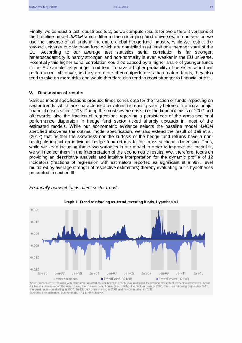
Various model specifications produce times series data for the fraction of funds impacting on sector trends, which are characterised by values increasing shortly before or during all major financial crises since 1995. During the most severe crisis, i.e. the financial crisis of 2007 and afterwards, also the fraction of regressions reporting a persistence of the cross-sectional performance dispersion in hedge fund sector ticked sharply upwards in most of the estimated models. While our econometric evidence selects the baseline model 4MOM specified above as the optimal model specification, we also extend the result of Bali et al. (2012) that neither the skewness nor the kurtosis of the hedge fund returns have a non-negligible impact on individual hedge fund returns to the cross-sectional dimension. Thus, while we keep including those two variables in our model in order to improve the model fit, we will neglect them in the interpretation of the econometric results. We, therefore, focus on providing an descriptive analysis and intuitive interpretation for the dynamic profile of 12 indicators (fractions of regression with estimators reported as significant at a 99% level multiplied by average strength of respective estimators) thereby evaluating our 4 hypotheses presented in section III.
Sectorially relevant funds affect sector trends
Graph 1: Trend reinforcing vs. trend reverting funds, Hypothesis 1
-0.025
-0.015
-0.005
0.005
0.015
0.025
Jan-95 Jan-97 Jan-99 Jan-01 Jan-03 Jan-05 Jan-07 Jan-09 Jan-11 Jan-13
crisis situations TrendReinf (B21>0) TrendRevert (B21<0)
Note: Fraction of regressions with estimators reported as significant at a 99% level multiplied by average strength of respective estimators. Areas for financial crises report the Asian crisis, the Russian default crisis (also LTCM), the doctom crisis of 2000, the crisis following Septmeber 9-11, the great recession starting in 2007, the EU debt crisis starting in 2009 and its continuation in 2012. Sources: Barclayhedge, Eurekahedge, TASS, HFR, ESMA.

ESMA Working Paper No. 2, 2015 15
The indicator TrendReinf, depicted in Graph 1, matches all financial crisis times observed with either a sharp up-ward jump at their beginnings or already before those actually start. The indicator TrenRevert reacts either simultaneously or slightly delayed and displays marginally higher persistence. Fluctuations in both measures are mainly driven by the respective fractions of funds with significant estimators, while the strength of those estimators is the main force behind increases in the level of both indicators in the second half of the sample period (cf. Appendix C.1). The only period showing higher levels in the measure not occurring during any financial crisis, i.e. the period in between 2002-2005, fits with the period of increased probabilities for hedge funds to experience poor performance rates reported in Chan et al. (2005). While these features remain broadly unchanged, if the length of the rolling window is extended, the measures’ reactiveness and the levels of their fluctuations are reduced (cf. Appendix D.3). Hence the qualitative results obtained do not raise any objection against the specification of 36 observations as an adequate length for the rolling window regressions.
However, both indicators display fluctuations in between 2001 and 2005 not related to stress in wider financial markets. Apparently one particular driver could include the massive reductions of the Federal Reserve Funds rate in 2001 and its low levels until autumn 2004, in particular as within this period the hedge fund industry realized a period of low volatility and very moderate levels in rate of returns. Thus, hedge funds anticipating the change in interest levels tended to partially correct the market downward trend in the beginning of this particular period, while those anticipating the later increase in 2004 corrected the still conservative sector trend in the second part of that period.
Trend reinforcing funds represent strategies which reconfirm the prevailing pattern of returns in the hedge fund industry. Thereby they tend to have a destabilising effect by corroborating potentially existing deviations from fundamentals. Trend reverting funds, on the other hand, form the complement with strategies performing contrary to the sector’s average performance. While, on the level of econometric analytics, our model does not provide specific economic factors driving this classification, an indicative interpretation is still worthwhile. Thus, in particular in times of market distress margin spirals, default chains and supply restrictions on liquidity probably reinforce the influence of trend reinforcing funds on the entire hedge fund sector. The potential use of correlated implicit or explicit benchmarks adds another source of explanation.20 The mitigating influence of trend reverting funds is most likely due to successful exploitation of strategies speculating synthetically against the market direction, such as global macro, commodity trading advisors/managed futures and relative value strategies, which particularly go along with high leverage21 and dynamic trading strategies.22 In particular, the dynamic profile illustrates that the influence of trend reinforcing fund increases earlier than that of trend reverting funds, as the first ones lead the general downturn to markets by taking a trigger position or an early propagation position, while the latter react to the materializing stress by decoupling in returns from weak asset market segments.
The relative increase in the number of trend reinforcing funds, observed since 2003 (cf. Appendix C.1), points to a stronger homogenization of performance movements in the hedge fund sector, as more and more funds act as positively correlated drivers for the industry. This trend goes along with tremendous growth in the size of the industry since 2003 and might be driven by the decreasing capacity to generate excess returns experienced by older and
20 Similar mechanisms have been discussed for funds specialised on emerging markets in Miyajima and Shim (2014).
21 This holds according to FCA (2014) e.g. for funds with UK licenses.
22 Trading strategies of global macro funds and commodity trading advisors appear to be more flexible, displayed by more volatile correlations to general asset market performance, than those of hedge funds following other strategies. This feature is discussed in more detail in Pictet (2014).
ESMA Working Paper No. 2, 2015 16
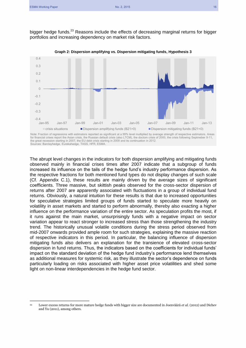
bigger hedge funds.23 Reasons include the effects of decreasing marginal returns for bigger portfolios and increasing dependency on market risk factors.
Graph 2: Dispersion amplifying vs. Dispersion mitigating funds, Hypothesis 3
The abrupt level changes in the indicators for both dispersion amplifying and mitigating funds observed mainly in financial crises times after 2007 indicate that a subgroup of funds increased its influence on the tails of the hedge fund’s industry performance dispersion. As the respective fractions for both mentioned fund types do not display changes of such scale (Cf. Appendix C.1), these results are mainly driven by the average sizes of significant coefficients. Three massive, but skittish peaks observed for the cross-sector dispersion of returns after 2007 are apparently associated with fluctuations in a group of individual fund returns. Obviously, a natural intuition for these results is that due to increased opportunities for speculative strategies limited groups of funds started to speculate more heavily on volatility in asset markets and started to perform abnormally, thereby also exacting a higher influence on the performance variation of the entire sector. As speculation profits the most, if it runs against the main market, unsurprisingly funds with a negative impact on sector variation appear to react stronger to increased stress than those strengthening the industry trend. The historically unusual volatile conditions during the stress period observed from mid-2007 onwards provided ample room for such strategies, explaining the massive reaction of respective indicators in this period. In particular, the balancing influence of dispersion mitigating funds also delivers an explanation for the transience of elevated cross-sector dispersion in fund returns. Thus, the indicators based on the coefficients for individual funds’ impact on the standard deviation of the hedge fund industry’s performance lend themselves as additional measures for systemic risk, as they illustrate the sector’s dependence on funds particularly loading on risks associated with higher asset price volatilities and shed some light on non-linear interdependencies in the hedge fund sector.
23 Lower excess returns for more mature hedge funds with bigger size are documented in Joenväärä et al. (2012) and Dichev
and Yu (2011), among others.
-0.4
-0.3
-0.2
-0.1
0
0.1
0.2
0.3
0.4
Jan-95 Jan-97 Jan-99 Jan-01 Jan-03 Jan-05 Jan-07 Jan-09 Jan-11 Jan-13
crisis situations Dispersion amplifying funds (B21>0) Dispersion mitigating funds (B21<0)
Note: Fraction of regressions with estimators reported as significant at a 99% level multiplied by average strength of respective estimators. Areas for financial crises report the Asian crisis, the Russian default crisis (also LTCM), the doctom crisis of 2000, the crisis following Septmeber 9-11, the great recession starting in 2007, the EU debt crisis starting in 2009 and its continuation in 2012. Sources: Barclayhedge, Eurekahedge, TASS, HFR, ESMA.
ESMA Working Paper No. 2, 2015 17
Sectorially vulnerable funds are affected by sector trends
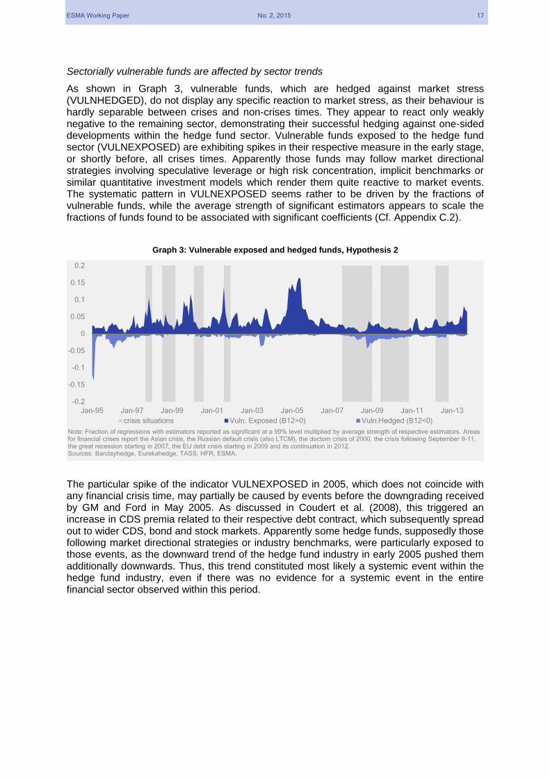
As shown in Graph 3, vulnerable funds, which are hedged against market stress (VULNHEDGED), do not display any specific reaction to market stress, as their behaviour is hardly separable between crises and non-crises times. They appear to react only weakly negative to the remaining sector, demonstrating their successful hedging against one-sided developments within the hedge fund sector. Vulnerable funds exposed to the hedge fund sector (VULNEXPOSED) are exhibiting spikes in their respective measure in the early stage, or shortly before, all crises times. Apparently those funds may follow market directional strategies involving speculative leverage or high risk concentration, implicit benchmarks or similar quantitative investment models which render them quite reactive to market events. The systematic pattern in VULNEXPOSED seems rather to be driven by the fractions of vulnerable funds, while the average strength of significant estimators appears to scale the fractions of funds found to be associated with significant coefficients (Cf. Appendix C.2).
Graph 3: Vulnerable exposed and hedged funds, Hypothesis 2
The particular spike of the indicator VULNEXPOSED in 2005, which does not coincide with any financial crisis time, may partially be caused by events before the downgrading received by GM and Ford in May 2005. As discussed in Coudert et al. (2008), this triggered an increase in CDS premia related to their respective debt contract, which subsequently spread out to wider CDS, bond and stock markets. Apparently some hedge funds, supposedly those following market directional strategies or industry benchmarks, were particularly exposed to those events, as the downward trend of the hedge fund industry in early 2005 pushed them additionally downwards. Thus, this trend constituted most likely a systemic event within the hedge fund industry, even if there was no evidence for a systemic event in the entire financial sector observed within this period.
-0.2
-0.15
-0.1
-0.05
0
0.05
0.1
0.15
0.2
Jan-95 Jan-97 Jan-99 Jan-01 Jan-03 Jan-05 Jan-07 Jan-09 Jan-11 Jan-13
crisis situations Vuln. Exposed (B12>0) Vuln.Hedged (B12<0)
Note: Fraction of regressions with estimators reported as significant at a 99% level multiplied by average strength of respective estimators. Areas for financial crises report the Asian crisis, the Russian default crisis (also LTCM), the doctom crisis of 2000, the crisis following September 9-11, the great recession starting in 2007, the EU debt crisis starting in 2009 and its continuation in 2012.Sources: Barclayhedge, Eurekahedge, TASS, HFR, ESMA.
ESMA Working Paper No. 2, 2015 18
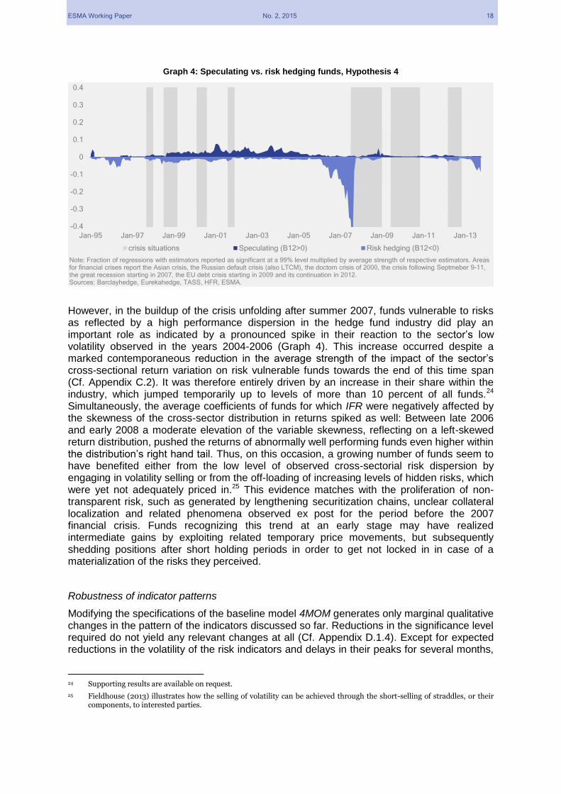
Graph 4: Speculating vs. risk hedging funds, Hypothesis 4
However, in the buildup of the crisis unfolding after summer 2007, funds vulnerable to risks as reflected by a high performance dispersion in the hedge fund industry did play an important role as indicated by a pronounced spike in their reaction to the sector’s low volatility observed in the years 2004-2006 (Graph 4). This increase occurred despite a marked contemporaneous reduction in the average strength of the impact of the sector’s cross-sectional return variation on risk vulnerable funds towards the end of this time span (Cf. Appendix C.2). It was therefore entirely driven by an increase in their share within the industry, which jumped temporarily up to levels of more than 10 percent of all funds.24 Simultaneously, the average coefficients of funds for which IFR were negatively affected by the skewness of the cross-sector distribution in returns spiked as well: Between late 2006 and early 2008 a moderate elevation of the variable skewness, reflecting on a left-skewed return distribution, pushed the returns of abnormally well performing funds even higher within the distribution’s right hand tail. Thus, on this occasion, a growing number of funds seem to have benefited either from the low level of observed cross-sectorial risk dispersion by engaging in volatility selling or from the off-loading of increasing levels of hidden risks, which were yet not adequately priced in.25 This evidence matches with the proliferation of non-transparent risk, such as generated by lengthening securitization chains, unclear collateral localization and related phenomena observed ex post for the period before the 2007 financial crisis. Funds recognizing this trend at an early stage may have realized intermediate gains by exploiting related temporary price movements, but subsequently shedding positions after short holding periods in order to get not locked in in case of a materialization of the risks they perceived.
Robustness of indicator patterns
Modifying the specifications of the baseline model 4MOM generates only marginal qualitative changes in the pattern of the indicators discussed so far. Reductions in the significance level required do not yield any relevant changes at all (Cf. Appendix D.1.4). Except for expected reductions in the volatility of the risk indicators and delays in their peaks for several months,
24 Supporting results are available on request.
25 Fieldhouse (2013) illustrates how the selling of volatility can be achieved through the short-selling of straddles, or their components, to interested parties.
-0.4
-0.3
-0.2
-0.1
0
0.1
0.2
0.3
0.4
Jan-95 Jan-97 Jan-99 Jan-01 Jan-03 Jan-05 Jan-07 Jan-09 Jan-11 Jan-13
crisis situations Speculating (B12>0) Risk hedging (B12<0)
Note: Fraction of regressions with estimators reported as significant at a 99% level multiplied by average strength of respective estimators. Areas for financial crises report the Asian crisis, the Russian default crisis (also LTCM), the doctom crisis of 2000, the crisis following Septmeber 9-11, the great recession starting in 2007, the EU debt crisis starting in 2009 and its continuation in 2012. Sources: Barclayhedge, Eurekahedge, TASS, HFR, ESMA.

ESMA Working Paper No. 2, 2015 19
variations in the length of the rolling window of baseline model 4MOM do not severely impact on our results (Cf. Appendix D.1.2). Modifications of the model’s lag length, however, result in qualitative changes. Increasing the number of lags to two severely reduces the models’ ability to identify financial crisis times, as in particular the peaks occurring before 2003 are smoothed out and do not longer match clearly with times of stress in financial markets. An alternative modification with a lag length of three and a rolling window length of 48 months yields results more similar to those of the baseline model, even if both EU debt crises events at the end of our reporting sample do not appear to be spotted by the indicators (Cf. Appendix D.1.1).
Varying the model specification with respect to the set of endogenous variables does not produce any changes in the measures’ dynamic patterns which would impose challenges to the model’s robustness. Models in which the cross-sectional return distribution of the hedge fund sector is represented by a set of percentiles tend to produce less volatile and less reactive indicators. Models using a smaller set of moments or percentiles compared to the baseline model display similar, but less volatile indicator patterns than their counterparts with larger sets of endogenous variables. Thus, the chosen baseline model seems to be superior in terms of signalling power, while its main message remains quite robust with respect to changes in the representation of the hedge fund’s sector cross-sectional heterogeneity. Additionally, symmetric models, i.e. models using the information contained in the left and right side of the hedge’ fund sector’s performance distribution similarly, tend to replicate the qualitative results obtained from model 4MOM relatively closely. Asymmetric models, i.e. those which factor in only information from the right-hand side of the distribution, however, appear to be distorted, as the estimators for the coefficients of the mean potentially attract variation from fund return series which would be allocated in symmetric settings to lower quantiles or dispersion measures. Thus, in general, asymmetric models identify crisis times less clearly and display less volatility than their symmetric counterparts (cf. Appendix D.3).
Similarly, our qualitative results turn out to be quite insensitive to a change in the universe from the entire global hedge fund industry to its EU subset. Comparing equivalent indicators for both universes, we find that the indicator for trend reinforcing funds and the indicator for trend reverting funds is in general more volatile for the EU universe, while the average levels for both indicators hardly differ at all. However, while the EU indicator for trend reinforcing funds misses several crises times in the first half of the reporting sample, the EU indicator for trend reverting funds reacts stronger than its global equivalent during two out of three crises times after 2005. Of particular interest is also the difference in Q4 2005. In this quarter some EU trend reinforcing hedge funds turned out to have a strong negative impact on the industry, potentially reacting to downward shift in US equity markets in October 2005. Moreover, as already pointed out in Section 4, the EU universe is composed of younger funds, which tend to be outperformers, also due to accepting higher risks. Hence, the EU sample should be more sensitive to financial stress, which is indeed indicated by the stronger reactions of our two indicators within the EU sample. Nevertheless, except for the mentioned differences, the general pattern of the indicators remains similar, also displayed by correlations in between the EU and global series which are with 0.42 for trend reinforcing and 0.35 for trend reverting funds clearly in the positive range, despite the occasional substantial deviations in the respective indicators.
Additional support for the robustness of our models stems from the fact that we can reconfirm some research results found by the previous literature. Thus, we employ the methodology presented in Section III to analyse serial correlation in the hedge fund sector’s mean returns, implying a non-zero first diagonal element in the coefficient matrix b22. Regressions resulting in significant negative first diagonal elements of the estimator b22 (< 0) are interpreted as evidence of receding systemic risk and regressions resulting in significant positive first diagonal elements of the estimator b22 (> 0) as evidence of receding systemic risk. Both indicators (cf. Appendix D.6) are characterized by several striking peaks driven by massive fluctuations in the fractions of regressions with significant estimators. The average

ESMA Working Paper No. 2, 2015 20
levels of those significant estimators present are remarkably stable over time and hoover around the value 1. However, the ratios of funds for which the model detects positive serial autocorrelations for the average return of the hedge fund sector exceed those with negative coefficients by far. Hence, positive autocorrelation prevails, even if there are also some periods of pure negative autocorrelation. While the sparseness of reactions in the two indicators does not suggest any particular role in the identification of systemic risk, the prevalence of positive autocorrelation patterns is reconfirmed by several studies which report for the hedge fund sector performance persistence on the industry or strategy level.
Complementarily, we investigate the presence of serial correlation in the sectorial standard deviation of hedge fund returns, as indicated by a non-zero second diagonal element in b22. Regressions generating significant second diagonal elements of the estimator b22 are interpreted as evidence for preservation of volatility and/or risks within the sector. Negatively significant estimators (<0) emphasize the volatility character, which implies dynamic risks, while positive ones point out the build-up of higher sector dispersion implying higher probabilities for unsustainable developments in part of the industry. Both indicators for the preservation or mitigation of performance volatility (cf. Appendix D.6) hardly show any amplitude at all, since for most periods either none or only a tiny fraction of significant coefficients are found. However, there are two noteworthy exceptions: In early 1997 almost all fund regressions result in a negative autocorrelation of return variances within the hedge funds sector, thus implying high levels of volatility. This pattern holds throughout the first 3 quarters of 1997.26 Similarly, in September 2007 almost 70% of all fund regressions reconfirm a positive autocorrelation in the sector’s return variance, which fades almost completely away after only one month. Hence, while episodes of serial correlation in the sector-wide variation of hedge fund returns exist, they are relatively rare and do not hold for prolonged time periods. The finding of Akkay et al. (2012) that so-called crash states, i.e. occurrences of negative mean returns and high volatilities, are rare and normally not persistent are thus reconfirmed by our results.
Finally, we compute for the baseline model 4MOM the fractions of funds leaving the existent group of funds identified as relevant ones and the ones of funds newly joining this group (Appendix D.5). Both measures are volatile over time, but are on average close to 30 percent. Hence, we conclude that the group of relevant funds is, given the substantive change of fund numbers over time and the low fund numbers in beginning, quite stable, with around 70% of funds remaining in this group for at least two consecutive months. Again this indicates a robustness of the proposed indicators for systemic risk.
VI. Conclusions
Based on the proposition that intra-sectorial interdependencies in the hedge-fund sector should show up in the cross-sectional distribution of hedge fund returns, we propose indicators for the monitoring of systemic risks or stress within this industry. To this purpose we built a large set of VAR-models regressing realisations of individual hedge fund returns and measures for the cross-sectional performance distribution of the entire industry on their past materializations and a set of exogenous variables. We use sector-wide aggregations of significant coefficients obtained from those regressions, to construct proxy measures depicting the effects of individual funds on other funds and vice versa.
Our proposed indicators for the effects of sectorially relevant funds on sector trends (cf. Graph 1) appear to be sensitive to all identified stress periods for the hedge fund sector. Hence we argue that the two proxies together might be adequate measures for systemic risk and/or stress in the hedge fund industry. These results are qualitatively robust to changes in the underlying regression models including modifications of lag lengths, variations in sample
26 Note the time overlap with the Asian financial crisis starting in July 1997.

ESMA Working Paper No. 2, 2015 21
sizes for the individual regressions, application of different significance levels for coefficients identified as significant and alterations in the set of the model’s set of endogenous variables. Even changes in the underlying fund universe from the global industry to the EU industry do not change qualitative results materially. Moreover, the group of funds identified as relevant ones experiences, given the strong increase in fund numbers over time, only a moderate change of its composition, as on average 70% percent of funds identified as relevant in a given period stay in this group also within the next period. We interpret all this evidence as strength of the proposed indicators, because marginal changes in the underlying methodologies do not impact on their indication of the level of systemic risks. We do, however, not claim any predictive power for our indicators, as the low frequencies and the relatively small observation horizons used do not suffice to allow for the econometric strength needed to engage in prediction or forecasting. Therefore, we assign only a signalling power, but no forecasting power to our indicators
We would like to emphasize a few additional methodological strengths which are characteristic for our proposed measures. Firstly, the underlying methodology is quite versatile, allowing e.g. for future rolling out of the same measure over different segments of the fund industry such as the mutual fund industry as well as money market funds. Secondly, the use of second and higher moments in our baseline model, or alternatively of quantiles in other model versions, factors in non-linear relationships stemming from fat-tailed return distributions, leveraged investment positions and the widespread use of derivatives within the industry. Thirdly, we separate spill-over effects and sector-trend effects from persistence in individual fund returns which is frequently interpreted as an expression of managerial talent (alpha) as well as from other individual fund effects reflecting on institutional properties which are in the literature frequently lumped together in the individual fixed effect of the fund. Finally, similar as a rolling network analysis, we allow for a dynamic profiling of systemic risk contribution over time thereby explicitly acknowledging the potential for compositional and structural changes in the fund industry such as the surge and the demise of individual entities’ systemic impact.
We acknowledge that for the time being our proposed measures are non-informative on any inter-sectorial systemic risks. However, as the econometric strategy employed controls for risk factors associated with several asset markets and risk categories, we plan to work on complementary measures for this area in the future. Similarly, as also pointed out above, we will be in the position to exploit individual performance persistence for measures of managerial alpha on an individual fund base as also provided in Kosowski et al. (2007).
The indicators and methodology proposed in this paper can be employed in order to identify vulnerabilities generated by subsections of the fund industry as well as individual entities. In particular, the virtue of being based on microeconomic data renders our proposal into a valuable complement to already existent approaches for the assessment of systemic risks in the fund industry.
ESMA Working Paper No. 2, 2015 22
VII. Bibliography
Abdi H. & Williams L. J., 2010. Principal component analysis. Wiley Interdisciplinary Reviews: Computational Statistics, Volume 2, Issue 4, pp. 433-459.
Acharya V.V., Pedersen L.H., Philippon T. & Richardson M.P., 2010. Measuring systemic risk.
NYU Stern, Working Paper.
Adrian T. & Brunnermeier M., 2009. CoVaR. Federal Reserve Bank of New York Staff Report,
No. 348.
Adrian T., 2007. Measuring risk in the hedge fund sector. Current Issues in Economics and
Finance, Volume 13, No 3.
Agarwal V. & Naik N., 2000. Multi-period performance persistence analysis of hedge funds.
Journal of Financial and Quantitative Analysis, Volume 35, No. 3, pp. 327-342.
Aiken A. L., Clifford C. P. & Ellis J., 2012. Do funds of hedge funds add value? Evidence from
their holdings. University of Kentucky, Working paper.
Akay O., Senyuz Z., & Yoldas E., 2013. Hedge fund contagion and risk-adjusted returns: A
markov-switching dynamic factor approach. Journal of Empirical Finance, Volume 22, pp. 16-
29.
Ammann M., Huber O., & Schmid M. 2013. Hedge fund characteristics and performance
persistence. European Financial Management, Volume 19, Issue 2, pp. 209-250.
Ang A., Gorovyy S. & van Inwegen G. B., 2011. Hedge fund leverage. Journal of Financial
Economics, Volume 102, No. 1, pp. 102-126.
Aragon G. & Martin J., 2009. A unique view of hedge fund derivatives usage: Safeguard or
speculation? Journal of Financial Economics, Volume 105, Issue 2. pp. 436–456.
Bali T. G., Brown S. J. & Caglayan M. O., 2012. Systematic risk and the cross section of
hedge fund returns. Journal of Financial Economics, Volume 106, Issue 1, pp. 114-131.
Ben-David I., Franzoni F. & Moussawi R., 2012. Hedge fund stock trading in the financial crisis
of 2007–2009. Review of Financial Studies, Volume 25, Issue 1, pp 1-54.
Billio M., Getmansky M. & Pelizzon L., 2010. Crises and hedge fund risk. University
Ca'Foscari of Venice, Dept. of Economics, Research Paper Series, 07-14.
Billio M., Getmansky M. & Pelizzon L., 2012. Dynamic risk exposures in hedge funds.
Computational Statistics and Data Analysis, Vol. 56, No. 11, pp. 3517-3532.
Billio M., Getmansky M., Lo A. W. & Pelizzon L., 2012. Econometric measures of
connectedness and systemic risk in the finance and insurance sectors. Journal of Financial
Economics, Vol. 104, No. 3, pp. 535–559.
Bisias D., Flood M. D., Lo A. W., & Valavanis S., 2012. A survey of systemic risk analytics.
Annual Review of Financial Economics, Issue 4, Volume 1, pp. 255-296
Bollerslev T., 1986. Generalized autoregressive conditional heteroskedasticity. Journal of
econometrics, Volume 31, Issue 3, pp. 307-327.

ESMA Working Paper No. 2, 2015 23
Boyson N. M., Stahel C. & Stulz R. M., 2010. Hedge fund contagion and liquidity shocks.
Journal of Finance, Volume 65, pp. 1789-1816.
Brownlees C. & Engle R. F., 2011. Volatility, correlation and tails for systemic risk
measurement. New York University - Stern School of Business, Working Paper.
Brunnermeier M. K. & Pedersen L. H., 2009. Market liquidity and funding liquidity. Review of
Financial Studies, Volume 22, pp. 2201-2238.
Brunnermeier M. K., 2009. Deciphering the 2007-2008 liquidity and credit crunch. Journal of
Economic Perspectives, Volume 23, pp. 77-100.
Bussiere M., Hoerove M. & Klaus B., 2014. Commonality in hedge fund returns: Driving
factors and implications. ECB Working Paper Series, No. 1658/March 2014.
Cao C., Chen Y., Liang B. & Lo A. W. 2013. Can hedge funds time market liquidity?. Journal
of Financial Economics, Volume 109, Issue 2, pp. 493-516.
Chan K. N., Getmansky M., Haas S. & Lo A. W., 2006. Systemic risk and hedge funds. The
Risks of Financial Institutions. Chicago and London: University of Chicago Press.
Christoffersen P., Goyenko R., Jacobs K. & Karoui M., 2014. Illiquidity premia in the equity
options market. University of Toronto, Working Paper.
Coudert, V. & Gex M., 2008. Contagion in the credit default swap market: The case of the GM
and Ford crisis in 2005. Journal of International Financial Markets, Institutions and Money,
Volume 20, Issue 2, pp. 109-134.
Dichev I. D., & Yu G. 2011. Higher risk, lower returns: What hedge fund investors really earn.
Journal of Financial Economics, Volume 100, Issue 2, pp. 248-263.
Dixon L., Clancy N., & Kumar K. B., 2011. Hedge funds and systemic risk. Rand Corporation.
Dudley E. & Nimalendran M., 2011. Margins and hedge fund contagion. Journal of Financial
and Quantitative Analysis, Volume 46, Issue 5, pp .1227-1257.
Dudley E. & Nimalendran M., 2012. Hedge fund leverage and financial fragility. Available at
SSRN 2023129.
Edelmann D., Fung W. & Hsieh D. A., 2013. Exploring uncharted territories of the hedge fund
industry: Empirical characteristics of mega hedge fund firms. Journal of Financial Economics,
Volume 109, Issue 3, pp. 734-758.
Edward F. R., 1999. Hedge funds and the collapse of long term capital management. Journal
of Economic Perspectives, Volume 13, Issue 2, pp. 189-210.
European Securities and Markets Authority, 2015. Trends, risks and vulnerabilities No. 1
March 2015.
Fieldhouse S., 2013. Trading volatility as an asset class: How hedge fund managers use
equity options. The Hedge Fund Journal, http://www.thehedgefundjournal.com/node/8332
Financial Conduct Authority, 2014. Hedge fund survey, FCA.

ESMA Working Paper No. 2, 2015 24
FSB-IOSCO, 2015. 2nd Consultative Document – Assessment Methodologies for Identifying
Non-Bank Non-Insurer Globally Systemically Important Financial Institutions.
Fung W. & Hsieh D. A., 1997. Empirical characteristics of dynamic trading strategies: The
case of hedge funds. Review of Financial Studies, Volume 10, pp. 275-302.
Fung W. & Hsieh D. A., 1999. A primer on hedge funds. Journal of Empirical Finance, Volume
6, pp. 53-58.
Fung W. & Hsieh D. A., 2001. The risk in hedge fund strategies: Theory and evidence from
trend followers. Review of Financial Studies, Volume 10, pp. 313-341.
Fung W., Hsieh D. A., Naik N. Y. & Ramadorai T., 2008. Hedge funds: performance, risk and
capital formation. Journal of Finance, Volume 63, pp. 1777-1803.
Getmansky M., 2012. The life cycle of hedge funds: Fund flows, size competition, and
performance. Quarterly Journal of Finance, Volume 2, Issue 1.
Getmansky M., Lo A. W. & Makarov I., 2004. An econometric model of serial correlation and
illiquidity in hedge fund returns. Journal of Financial Economics, Volume 74, pp. 529-609.
Hespeler F. & Witt C., 2014. The systemic dimension of hedge fund illiquidity and prime
brokerage. ESMA Working Paper Series, No. 2, 2014.
Huang X., Zhou H. & Zhu H, 2010. Assessing the systemic risk of a heterogeneous portfolio of
banks during the recent financial crisis. Bank for International Settlements, BIS Working Paper
No 296.
Joenväärä J., Kosowski R. & Tolonen P., 2012. Revisiting stylized facts about hedge funds.
EDHEC Working Paper.
Khandani A. E. & Lo A. W. 2011. Illiquidity premia in asset returns: an empirical analysis of
hedge funds, mutual funds, and US equity portfolios. The Quarterly Journal of Finance,
Volume 1, Issue 2, pp. 205-264.
King M. R. & Maier P., 2009. Hedge funds and financial stability: Regulating prime brokers will
mitigate systemic risks. Journal of Financial Stability, Volume 5, pp. 283-297.
Klaus B. & Rzepkowski B., 2009. Hedge funds and prime brokers: The role of funding risk.
EFA 2009 Bergen Meetings Paper.
Kosowski R., Naik N. Y. & Teo M., 2007. Do hedge fund deliver alpha? A Bayesian and
bootstrap analysis. Journal of Financial Economics, Volume 84, Issue 1, pp. 229-264.
Kruttli M., Patton A. J. & Ramadorai T., 2013. The impact of hedge funds on asset markets.
CEPR Discussion Paper No. DP10151, pp. 1-40.
Liu X. & Mello A. S., 2011. The fragile capital structure of hedge funds and the limits to
arbitrage. Journal of Financial Economics, Volume 102, pp. 491-506.
McGuire P. & Tsatsaronis K., 2008. Estimating hedge fund leverage. Bank for International
Settlements, BIS Working Paper No. 260.

ESMA Working Paper No. 2, 2015 25
Miyajima K. & Shim I., 2014. Asset managers in emerging market economies. Bank for
International Settlements, BIS Quarterly Review.
Patton A. J. & Ramadorai T., 2013. On the high-frequency dynamics of hedge fund risk
exposures. Journal of Finance, Volume 68, Issue 2, pp. 597–635.
Pictet Alternative Advisors SA, 2014. Hedge funds: the case for trading strategies. Pictet.
Zykaj B.B.., Sias R. & Turtle H. J., 2012. Hedge fund herding: The apologists' evidence.
Available at SSRN 2021344.
Roncalli T. & Weisang G., 2015, Asset management and systemic risk. Available at SSRN
2610174.
Sadka R, 2010. Liquidity risk and the cross-section of hedge-fund returns. Journal of Financial
Economics, Volume 98, Issue 1, pp. 54-71.
Sun Z., Wang A., & Zheng L., 2012. The road less travelled: Strategy distinctiveness and
hedge fund performance. Review of Financial Studies, Volume 25, Issue 1, pp. 96-143.
Teo M., 2011. The liquidity risk of liquid hedge funds. Journal of Financial Economics, Volume
100, Issue 1, pp. 24-44.

ESMA Working Paper No. 2, 2015 26
Appendix A. Model specifications
Model Name
Endogenous Variables for HF sector
Model specifications details
Lag Obs. Results
4MOM (Baseline model)
First 4 moments of distribution of fund returns: mean, standard deviation, skewness, kurtosis
1 60, 48 Presented in Appendix D. Results are also reported for the model with a specification of 1 lag, rolling window length 36 and maximal numbers of observations allowed to miss of 0, 5 and 10. For all other models only the value 10 is used.
1 36
2 60, 48, 36
3 60, 48
3 36 Data requirements for 110 estimators too high to be reliably estimated with 180 or less observations
2MOM First 2 moments of distribution of fund returns: mean, standard deviation
1, 2, 3
60, 48, 36 Presented in Appendix D
3PER Percentages of distribution of fund returns reflecting both tails of the distribution: 90%, 50%, 10%
1, 2 60, 48, 36 Presented in Appendix D
3 60, 48
3 36 Data requirements for 70 estimators too high to be reliably estimated with 144 or less observations
3PERASY Percentages of distribution of fund returns reflecting the upper tail of the distribution: 99%, 90%, 50%
1, 2 60, 48, 36 Presented in Appendix D
3 60, 48
3 36 Data requirements for 70 estimators too high to be reliably estimated with 144 or less observations
5PER Percentages of distribution of fund returns reflecting both tails of the distribution: 99%, 75% , 50%, 25%, 1%
1 60, 48, 36 Presented in Appendix D
2 60, 48
2 36 Data requirements for 114 estimators too high to be reliably estimated with 180 or less observations
3 60 Presented in Appendix D
3 48, 36 Data requirements for 140 estimators too high to be reliably estimated with 240 or less observations
5PERASY Percentages of distribution of fund returns reflecting the upper tail of the distribution:
1 60, 48, 36 Presented in Appendix D
2 60, 48
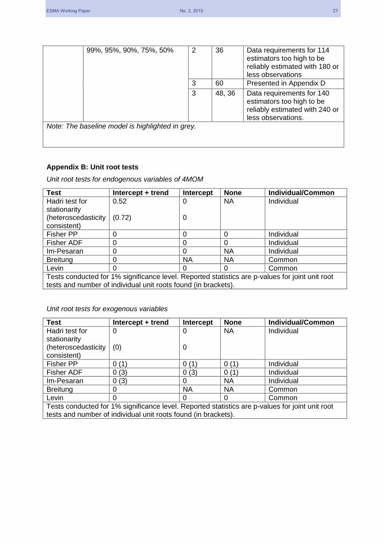
ESMA Working Paper No. 2, 2015 27
99%, 95%, 90%, 75%, 50% 2 36 Data requirements for 114 estimators too high to be reliably estimated with 180 or less observations
3 60 Presented in Appendix D
3 48, 36 Data requirements for 140 estimators too high to be reliably estimated with 240 or less observations.
Note: The baseline model is highlighted in grey.
Appendix B: Unit root tests
Unit root tests for endogenous variables of 4MOM
Test Intercept + trend Intercept None Individual/Common
Hadri test for stationarity (heteroscedasticity consistent)
0.52 (0.72)
0 0
NA Individual
Fisher PP 0 0 0 Individual
Fisher ADF 0 0 0 Individual
Im-Pesaran 0 0 NA Individual
Breitung 0 NA NA Common
Levin 0 0 0 Common
Tests conducted for 1% significance level. Reported statistics are p-values for joint unit root tests and number of individual unit roots found (in brackets).
Unit root tests for exogenous variables
Test Intercept + trend Intercept None Individual/Common
Hadri test for stationarity (heteroscedasticity consistent)
0 (0)
0 0
NA Individual
Fisher PP 0 (1) 0 (1) 0 (1) Individual
Fisher ADF 0 (3) 0 (3) 0 (1) Individual
Im-Pesaran 0 (3) 0 NA Individual
Breitung 0 NA NA Common
Levin 0 0 0 Common
Tests conducted for 1% significance level. Reported statistics are p-values for joint unit root tests and number of individual unit roots found (in brackets).

ESMA Working Paper No. 2, 2015 28
Appendix C: Additional Results
The following sections provide additional results used for the construction of the various indicators discussed in the main text. Specifically, the results for their two main components average coefficient strength and fraction of respective significant estimators are presented for the individual hypotheses discussed.
C.1 Sectorially relevant funds affect sector trends
Econometric evidence shows that the accuracy of the indicators “TrendReinf” and “TrendRevert” to capture crisis periods is mainly driven by the fractions of trend reinforcing and reverting funds. The average levels of significant coefficients identified remains, in particular for trend reverting funds, less volatile than their respective fractions. Analysing the dependence of the second moment of the distribution of hedge fund returns across the sector and the individual hedge fund returns, the available evidence shows that the average strength of the respective coefficients drives the respective indicators much stronger than in case of the first moment. Of special interest is the marked jump in the size and volatility of the average coefficient size in last third of the sample, which, as discussed in the main text, appears to indicate an increased engagement of some funds in speculative investment strategies.
Trend reinforcing and reverting funds: Hypothesis 1
Dispersion amplifying vs. dispersion mitigating funds: Hypothesis 3
-1.5
-1
-0.5
0
0.5
1
1.5
Jan-95 Jan-99 Jan-03 Jan-07 Jan-11
crisis situations TrendReinf (B21>0) TrendRevert (B21<0)
Note: Average strength of respective significant estimators. Areas for financial crises report the Asian crisis, the Russian default crisis (also LTCM), the doctom crisis of 2000, the crisis following Septmeber 9-11, the great recession starting in 2007, the EU debt crisis starting in 2009 and its continuation in 2012.Sources: Barclayhedge, Eurekahedge, TASS, HFR, ESMA.
0
0.01
0.02
0.03
0.04
0.05
Jan-95 Jan-99 Jan-03 Jan-07 Jan-11
crisis situations TrendReinf (B21>0) TrendRevert (B21<0)Note: Fractions of respective significant estimators. Areas for financial crises report the Asian crisis, the Russian default crisis (also LTCM), the doctom crisis of 2000, the crisis following Septmeber 9-11, the great recession starting in 2007, the EU debt crisis starting in 2009 and its continuation in 2012.Sources: Barclayhedge, Eurekahedge, TASS, HFR, ESMA.
-10-8-6-4-202468
10
Jan-95 Jan-99 Jan-03 Jan-07 Jan-11crisis situationsDispersion amplifying funds (B21>0)Dispersion mitigating funds (B21<0)
Note: Average strength of respective significant estimators. Areas for financial crises report the Asian crisis, the Russian default crisis (also LTCM), the doctom crisis of 2000, the crisis following Septmeber 9-11, the great recession starting in 2007, the EU debt crisis starting in 2009 and its continuation in 2012.Sources: Barclayhedge, Eurekahedge, TASS, HFR, ESMA.
0
0.01
0.02
0.03
0.04
0.05
0.06
0.07
Jan-95 Jan-99 Jan-03 Jan-07 Jan-11
crisis situationsDispersion amplifying funds (B21>0)Dispersion mitigating funds (B21<0)
Note: Fractions of respective significant estimators. Areas for financial crises report the Asian crisis, the Russian default crisis (also LTCM), the doctom crisis of 2000, the crisis following Septmeber 9-11, the great recession starting in 2007, the EU debt crisis starting in 2009 and its continuation in 2012.Sources: Barclayhedge, Eurekahedge, TASS, HFR, ESMA.
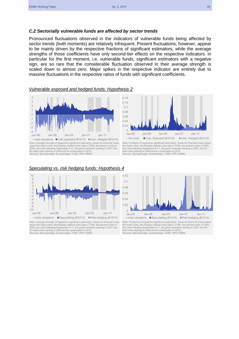
ESMA Working Paper No. 2, 2015 29
C.2 Sectorially vulnerable funds are affected by sector trends
Pronounced fluctuations observed in the indicators of vulnerable funds being affected by sector trends (both moments) are relatively infrequent. Present fluctuations, however, appear to be mainly driven by the respective fractions of significant estimators, while the average strengths of those coefficients have only second-tier effects on the respective indicators. In particular for the first moment, i.e. vulnerable funds, significant estimators with a negative sign, are so rare that the considerable fluctuation observed in their average strength is scaled down to almost zero. Major spikes in the respective indicator are entirely due to massive fluctuations in the respective ratios of funds with significant coefficients.
Vulnerable exposed and hedged funds: Hypothesis 2
Speculating vs. risk hedging funds: Hypothesis 4
-4
-3
-2
-1
0
1
2
3
4
Jan-95 Jan-99 Jan-03 Jan-07 Jan-11
crisis situations Vuln exposed (B12>0) Vuln. Hedged (B12<0)
Note: Average strength of respective significant estimators. Areas for financial crises report the Asian crisis, the Russian default crisis (also LTCM), the doctom crisis of 2000, the crisis following Septmeber 9-11, the great recession starting in 2007, the EU debt crisis starting in 2009 and its continuation in 2012.Sources: Barclayhedge, Eurekahedge, TASS, HFR, ESMA.
0
0.02
0.04
0.06
0.08
0.1
0.12
0.14
Jan-95 Jan-99 Jan-03 Jan-07 Jan-11
fin crisis Vuln. Exposed (B12>0) Vuln. Hedged (B12<0)
Note: Fractions of respective significant estimators. Areas for financial crises report the Asian crisis, the Russian default crisis (also LTCM), the doctom crisis of 2000, the crisis following September 9-11, the great recession starting in 2007, the EU debt crisis starting in 2009 and its continuation in 2012.Sources: Barclayhedge, Eurekahedge, TASS, HFR, ESMA.
-10
-8
-6
-4
-2
0
2
4
6
8
10
Jan-95 Jan-99 Jan-03 Jan-07 Jan-11
crisis situations Speculating (B12>0) Risk hedging (B12<0)
Note: Average strength of respective significant estimators. Areas for financial crises report the Asian crisis, the Russian default crisis (also LTCM), the doctom crisis of 2000, the crisis following Septmeber 9-11, the great recession starting in 2007, the EU debt crisis starting in 2009 and its continuation in 2012.Sources: Barclayhedge, Eurekahedge, TASS, HFR, ESMA.
0
0.02
0.04
0.06
0.08
0.1
0.12
Jan-95 Jan-99 Jan-03 Jan-07 Jan-11
crisis situations Speculating (B12>0) Risk hedging (B12<0)
Note: Fractions of respective significant estimators. Areas for financial crises report the Asian crisis, the Russian default crisis (also LTCM), the doctom crisis of 2000, the crisis following Septmeber 9-11, the great recession starting in 2007, the EU debt crisis starting in 2009 and its continuation in 2012.Sources: Barclayhedge, Eurekahedge, TASS, HFR, ESMA.

ESMA Working Paper No. 2, 2015 30
Appendix D: Robustness checks
This appendix provides the results of several econometric tests conducted in order to assess and support the robustness of the model presented.
D.1 Models with same set of endogenous variables as baseline model 4MOM
In terms of our three main test statistics the baseline model 4MOM outperforms all alternatives preserving the set of endogenous variables chosen, as clearly indicated by the dominance of negative differences in between the test statistics for the baseline model and those for the respective alternative models. Only a model variant with the same specification as 4MOM, but allowing for less missing observations within the 36 months horizon, appears to perform superior in terms of the three main test statistics. However, this superiority does not hold in terms of reliability proxies (Cf. C.1.3.). More details on variations in specific parameters are given below.
D.1.1 Selection of lag length
The lag length selection follows the idea of maintaining a nested model structure, i.e. a model with a prefixed number of lags, while allowing for endogenous selection of lags. As the average of the chosen lags across the individual fund regressions fluctuates within a corridor of 0 to 1.8 with values being considerably higher in the second half of the sample period, a lag length of 1 has been selected. Apparently this does not fully reflect the heterogeneity of lag structures optimal for the individual regressions, as some test statistics indicated for some fund regression an optimal lag length of zero while alternative statistics indicate for other fund regressions an optimal lag length of 3. However, balancing the attempt to implement a joint, nested model for all funds against the optimal fit for each individual fund regression, a length of one lag appears to strike a good and reliable compromise. As the fraction of funds failing the test for normality increases with the number of lags, this criterion delivers further support for the choice of a VAR model with one lag.
-0.3
-0.25
-0.2
-0.15
-0.1
-0.05
0
0.05
0.1
Serial correlation testsfailed
Heteroscedasticity testfailed
Normality tests failed
1 lag. 60 obs., 10 miss. 1 lag, 48 obs., 10 miss. 1 lag, 36 obs., 0 miss.
1 lag, 36 obs., 5 miss. 2 lags, 36 obs., 10 miss. 2 lags, 60 obs., 10 miss.
2 lags, 48 obs., 10 miss. 3 lags, 60 obs., 10 miss. 3 lags, 48 obs., 10 miss.
Note: Absolute deviations of baseline model 4MOM average test statistics from those of respective alternative models, percentage points.Sources: Barclayhedge, Eurekahedge, TASS, HFR, ESMA.

ESMA Working Paper No. 2, 2015 31
D.1.2 Selection of rolling window
For the baseline model 4MOM, an extension of the length of the rolling windows implies an increase in the fraction of funds failing the homoscedasticity test, in particular for the model using 48 observations. This is accompanied by a rise in the fraction of funds failing the test for absence of serial correlation and a higher ratio of funds for which non-normality is an issue. Thus all three tests point to the selection of the model with the shorter rolling window. The substantial ratio of regressions for which normality of residuals can be rejected, could pose a problem, as non-normal residuals have the potential to distort t-statistics by lowering those. However, it should be noted that especially for small samples the Jarque-Bera test tends to inflate the number of cases for which normality is rejected, thus mitigating the mentioned distortion. Based on this argument we disregard this problem.
0
0.2
0.4
0.6
0.8
1
1.2
1.4
1.6
1.8
2
Jan-95 Jan-97 Jan-99 Jan-01 Jan-03 Jan-05 Jan-07 Jan-09 Jan-11 Jan-13
MIX LM
Note: Average number of lag lenghts chosen for VAR modelaccording to criteria employed. LM= lagrange multiplier, MIX= average of lenght chosen according to LM, log-likelihood, forecast error, Akaike information criterion, Schwartz information criterion and Hannan-Quinn information criterion.Sources: ESMA.
0
0.05
0.1
0.15
0.2
0.25
0.3
Jan-95 Jan-97 Jan-99 Jan-01 Jan-03 Jan-05 Jan-07 Jan-09 Jan-11 Jan-13
SCORFAIL 36M SCORFAIL 48M SCORFAIL 60M
Note: Fractions of regressions failed respective tests and average valued of test statistics for set of funds which failed. Sources: ESMA.
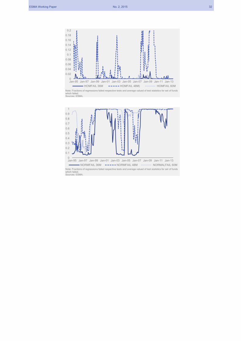
ESMA Working Paper No. 2, 2015 32
0
0.02
0.04
0.06
0.08
0.1
0.12
0.14
0.16
0.18
0.2
Jan-95 Jan-97 Jan-99 Jan-01 Jan-03 Jan-05 Jan-07 Jan-09 Jan-11 Jan-13
HOMFAIL 36M HOMFAIL 48M) HOMFAIL 60M
Note: Fractions of regressions failed respective tests and average valued of test statistics for set of funds which failed. Sources: ESMA.
0
0.1
0.2
0.3
0.4
0.5
0.6
0.7
0.8
0.9
1
Jan-95 Jan-97 Jan-99 Jan-01 Jan-03 Jan-05 Jan-07 Jan-09 Jan-11 Jan-13
NORMFAIL 36M NORMFAIL 48M NORMALFAIL 60M
Note: Fractions of regressions failed respective tests and average valued of test statistics for set of funds which failed. Sources: ESMA.
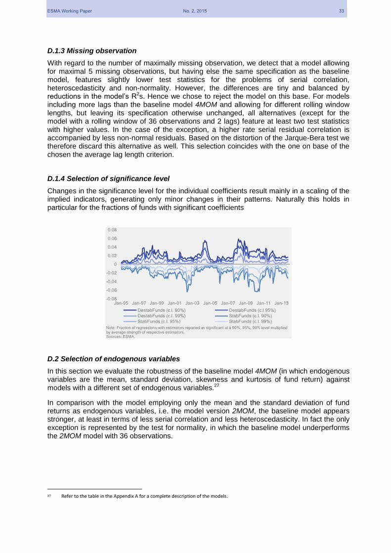
ESMA Working Paper No. 2, 2015 33
D.1.3 Missing observation
With regard to the number of maximally missing observation, we detect that a model allowing for maximal 5 missing observations, but having else the same specification as the baseline model, features slightly lower test statistics for the problems of serial correlation, heteroscedasticity and non-normality. However, the differences are tiny and balanced by reductions in the model’s R2s. Hence we chose to reject the model on this base. For models including more lags than the baseline model 4MOM and allowing for different rolling window lengths, but leaving its specification otherwise unchanged, all alternatives (except for the model with a rolling window of 36 observations and 2 lags) feature at least two test statistics with higher values. In the case of the exception, a higher rate serial residual correlation is accompanied by less non-normal residuals. Based on the distortion of the Jarque-Bera test we therefore discard this alternative as well. This selection coincides with the one on base of the chosen the average lag length criterion.
D.1.4 Selection of significance level
Changes in the significance level for the individual coefficients result mainly in a scaling of the implied indicators, generating only minor changes in their patterns. Naturally this holds in particular for the fractions of funds with significant coefficients
D.2 Selection of endogenous variables
In this section we evaluate the robustness of the baseline model 4MOM (in which endogenous variables are the mean, standard deviation, skewness and kurtosis of fund return) against models with a different set of endogenous variables.27
In comparison with the model employing only the mean and the standard deviation of fund returns as endogenous variables, i.e. the model version 2MOM, the baseline model appears stronger, at least in terms of less serial correlation and less heteroscedasticity. In fact the only exception is represented by the test for normality, in which the baseline model underperforms the 2MOM model with 36 observations.
27
Refer to the table in the Appendix A for a complete description of the models.
-0.08
-0.06
-0.04
-0.02
0
0.02
0.04
0.06
0.08
Jan-95 Jan-97 Jan-99 Jan-01 Jan-03 Jan-05 Jan-07 Jan-09 Jan-11 Jan-13
DestabFunds (c.l. 90%) DestabFunds (c.l 95%)
DestabFunds (c.l. 99%) StabFunds (c.l. 90%)
StabFunds (c.l. 95%) StabFunds (c.l. 99%)
Note: Fraction of regressions with estimators reported as significant at a 90%, 95%, 99% level multiplied by average strength of respective estimators.Sources: ESMA.
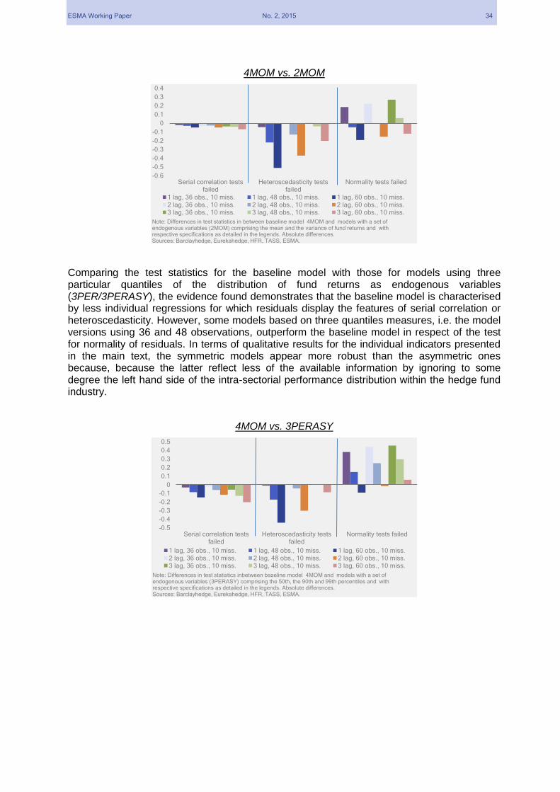
ESMA Working Paper No. 2, 2015 34
4MOM vs. 2MOM
Comparing the test statistics for the baseline model with those for models using three particular quantiles of the distribution of fund returns as endogenous variables (3PER/3PERASY), the evidence found demonstrates that the baseline model is characterised by less individual regressions for which residuals display the features of serial correlation or heteroscedasticity. However, some models based on three quantiles measures, i.e. the model versions using 36 and 48 observations, outperform the baseline model in respect of the test for normality of residuals. In terms of qualitative results for the individual indicators presented in the main text, the symmetric models appear more robust than the asymmetric ones because, because the latter reflect less of the available information by ignoring to some degree the left hand side of the intra-sectorial performance distribution within the hedge fund industry.
4MOM vs. 3PERASY
-0.6
-0.5
-0.4
-0.3
-0.2
-0.1
0
0.1
0.2
0.3
0.4
Serial correlation testsfailed
Heteroscedasticity testsfailed
Normality tests failed
1 lag, 36 obs., 10 miss. 1 lag, 48 obs., 10 miss. 1 lag, 60 obs., 10 miss.2 lag, 36 obs., 10 miss. 2 lag, 48 obs., 10 miss. 2 lag, 60 obs., 10 miss.3 lag, 36 obs., 10 miss. 3 lag, 48 obs., 10 miss. 3 lag, 60 obs., 10 miss.
Note: Differences in test statistics in between baseline model 4MOM and models with a set of endogenous variables (2MOM) comprising the mean and the variance of fund returns and with respective specifications as detailed in the legends. Absolute differences.Sources: Barclayhedge, Eurekahedge, HFR, TASS, ESMA.
-0.5
-0.4
-0.3
-0.2
-0.1
0
0.1
0.2
0.3
0.4
0.5
Serial correlation testsfailed
Heteroscedasticity testsfailed
Normality tests failed
1 lag, 36 obs., 10 miss. 1 lag, 48 obs., 10 miss. 1 lag, 60 obs., 10 miss.2 lag, 36 obs., 10 miss. 2 lag, 48 obs., 10 miss. 2 lag, 60 obs., 10 miss.3 lag, 36 obs., 10 miss. 3 lag, 48 obs., 10 miss. 3 lag, 60 obs., 10 miss.
Note: Differences in test statistics inbetween baseline model 4MOM and models with a set of endogenous variables (3PERASY) comprising the 50th, the 90th and 99th percentiles and with respective specifications as detailed in the legends. Absolute differences.Sources: Barclayhedge, Eurekahedge, HFR, TASS, ESMA.

ESMA Working Paper No. 2, 2015 35
4MOM vs. 3PER
Finally, a comparison of the baseline model’s test statistics with the ones of models using five quantiles of the distribution of fund returns as endogenous variables (5PER/5PERASY) illustrates that, again, the baseline model is characterised by less individual regressions exposed to issues stemming from serial correlation or heteroscedasticity in residuals. However, most models based on five quantiles measures perform better than the baseline model in respect to the test for normality of residuals. In terms of qualitative results for the individual indicators presented in the main text, the symmetric models appear again more robust than the asymmetric ones because, because the latter reflect less of the available information by ignoring to some degree the left hand side of the intra-sectorial performance distribution within the hedge fund industry.
4MOM vs. 5PERASY
-0.5
-0.4
-0.3
-0.2
-0.1
0
0.1
0.2
0.3
0.4
0.5
Serial correlation testsfailed
Homoschedasticity testsfailed
Normality tests failed
1 lag, 36 obs., 10 miss. 1 lag, 48 obs., 10 miss. 1 lag, 60 obs., 10 miss.2 lag, 36 obs., 10 miss. 2 lag, 48 obs., 10 miss. 2 lag, 60 obs., 10 miss.3 lag, 36 obs., 10 miss. 3 lag, 48 obs., 10 miss. 3 lag, 60 obs., 10 miss.
Note: Differences in test statistics inbetween baseline model 4MOM and models with a set of endogenous variables (3PER) comprising the 50th, the 90th and 10th percentiles and with respective specifications as detailed in the legends. Absolute differences.Sources: Barclayhedge, Eurekahedge, HFR, TASS, ESMA.
-0.2
-0.15
-0.1
-0.05
0
0.05
0.1
0.15
0.2
0.25
0.3
Serial correlation testsfailed
Heteroscedasticity testsfailed
Normality tests failed
1 lag, 36 obs., 10 miss. 1 lag, 48 obs., 10 miss. 1 lag. 60 obs., 10 miss.2 lags, 36 obs., 10 miss. 2 lags, 48 obs., 10 miss. 2 lags, 60 obs., 10 miss.3 lags, 48 obs., 10 miss. 3 lags, 60 obs., 10 miss.
Note: Differences in test statisitic in between baseline model 4MOM and models with a set of endogenous variabes (5PERASY) comprising the , 50th, 75th, 90th, 95th and 99th percentiles and with respective specifications as detailed in the legends. Absolute differences.Sources: Barclayhedge, Eurekahedge, TASS, HFR, ESMA.

ESMA Working Paper No. 2, 2015 36
4MOM vs. 5PER
D.3 Robustness of indicators
In this section we evaluate the robustness of our indicators in terms of changes of their dynamic patterns of our baseline model against different model specifications with respect to the set of endogenous variables (see Appendix A for the model naming conventions).
The model specifications where the sectorial return distribution is represented by the average and the standard deviation (2MOM) provide indicators, which are overall similar, in terms of reactiveness to crisis periods, to the baseline model. However, the indicators for the latter appear superior with regard to their reactiveness to crisis periods between 1995 and 2001.
The models, which capture the characteristics of the hedge fund sector return distribution through selected quantiles, appear to provide inferior indicators than the baseline model for all crisis periods. In the graphs below the indicators plotted refer to the element in the coefficient b21 associated with the 50th percentile.
Model 4MOM (left-hand side)/ Model 2MOM (right-end side)
-0.2
-0.15
-0.1
-0.05
0
0.05
0.1
0.15
0.2
0.25
0.3
Serial correlation testsfailed
Heteroscedasticity testsfailed
Normality tests failed
1 lag, 36 obs., 10 miss. 1 lag, 48 obs., 10 miss. 1 lag. 60 obs., 10 miss.2 lags, 36 obs., 10 miss. 2 lags, 48 obs., 10 miss. 2 lags, 60 obs., 10 miss.3 lags, 48 obs., 10 miss. 3 lags, 60 obs., 10 miss.
Note: Differences in test statisitic in between baseline model 4MOM and models with a set of endogenous variabes (5PER) comprising the 1st, 25th, 50th, 75th and 99th percentiles and with respective specifications as detailed in the legends. Absolute differences.Sources: Barclayhedge, Eurekahedge, TASS, HFR, ESMA.
-0.025
-0.015
-0.005
0.005
0.015
0.025
Jan-95 Jan-99 Jan-03 Jan-07 Jan-11
crisis situations TrendReinf (B21>0) TrendRevert (B21<0)
Note: Fraction of regressions with estimators reported as significant at a 99% level multiplied by average strength of respective estimators. Areas for financial crises report the Asian crisis, the Russian default crisis (also LTCM), the doctom crisis of 2000, the crisis following Septmeber 9-11, the great recession starting in 2007, the EU debt crisis starting in 2009 and its continuation in 2012. Sources: Barclayhedge, Eurekahedge, TASS, HFR, ESMA.
-0.025
-0.015
-0.005
0.005
0.015
0.025
Jan-95 Jan-99 Jan-03 Jan-07 Jan-11
crisis situations TrendReinf (B21>0) TrendRevert (B21<0)Note: Fraction of regressions with estimators reported as significant at a 99% level multiplied by average strength of respective estimators. Areas for financial crises report the Asian crisis, the Russian default crisis (also LTCM), the doctom crisis of 2000, the crisis following Septmeber 9-11, the great recession starting in 2007, the EU debt crisis starting in 2009 and its continuation in 2012. Sources: Barclayhedge, Eurekahedge, TASS, HFR, ESMA.

ESMA Working Paper No. 2, 2015 37
Model 3PER (left-hand side) / Model 3PERASY (right-end side)
Model 5PER (left-end side) / Model 5PERASY (right-end side)
D.4 Indicator based on EU sample
The graph displayed in this section reconfirms the robustness of the proposed indicators on relevant funds with respect to a change in the universe from the entire global hedge fund industry to its EU subset.
-0.025
-0.015
-0.005
0.005
0.015
0.025
Jan-95 Jan-99 Jan-03 Jan-07 Jan-11crisis situations TrendReinf (B21>0) TrendRevert (B21<0)
Note: Fraction of regressions with estimators reported as significant at a 99% level multiplied by average strength of respective estimators. Areas for financial crises report the Asian crisis, the Russian default crisis (also LTCM), the doctom crisis of 2000, the crisis following Septmeber 9-11, the great recession starting in 2007, the EU debt crisis starting in 2009 and its continuation in 2012. Sources: Barclayhedge, Eurekahedge, TASS, HFR, ESMA.
-0.025
-0.015
-0.005
0.005
0.015
0.025
Jan-95 Jan-99 Jan-03 Jan-07 Jan-11
crisis situations TrendReinf (B21>0) TrendRevert (B21<0)
Note: Fraction of regressions with estimators reported as significant at a 99% level multiplied by average strength of respective estimators. Areas for financial crises report the Asian crisis, the Russian default crisis (also LTCM), the doctom crisis of 2000, the crisis following Septmeber 9-11, the great recession starting in 2007, the EU debt crisis starting in 2009 and its continuation in 2012. Sources: Barclayhedge, Eurekahedge, TASS, HFR, ESMA.
-0.025
-0.015
-0.005
0.005
0.015
0.025
Jan-95 Jan-99 Jan-03 Jan-07 Jan-11
crisis situations TrendReinf (B21>0) TrendRevert (B21<0)
Note: Fraction of regressions with estimators reported as significant at a 99% level multiplied by average strength of respective estimators. Areas for financial crises report the Asian crisis, the Russian default crisis (also LTCM), the doctom crisis of 2000, the crisis following Septmeber 9-11, the great recession starting in 2007, the EU debt crisis starting in 2009 and its continuation in 2012.Sources: Barclayhedge, Eurekahedge, TASS, HFR, ESMA.
-0.03
-0.02
-0.01
0
0.01
0.02
0.03
Jan-95 Jan-97 Jan-99 Jan-01 Jan-03 Jan-05 Jan-07 Jan-09 Jan-11 Jan-13
crisis situations TrendReinf (B21>0) TrendRevert (B21<0)
Note: Fraction of regressions with estimators reported as significant at a 99% level multiplied by average strength of respective estimators. Areas for financial crises report the Asian crisis, the Russian default crisis (also LTCM), the doctom crisis of 2000, the crisis following Septmeber 9-11, the great recession starting in 2007, the EU debt crisis starting in 2009 and its continuation in 2012. Sources: Barclayhedge, Eurekahedge, TASS, HFR, ESMA.
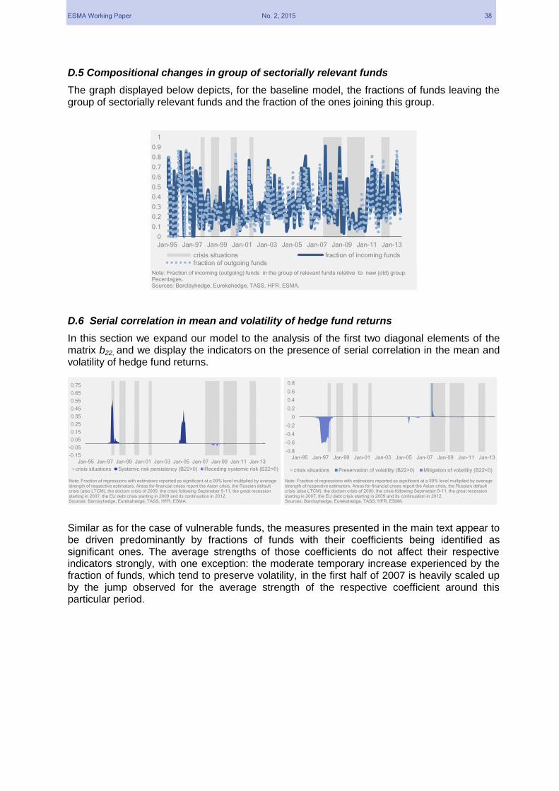
ESMA Working Paper No. 2, 2015 38
D.5 Compositional changes in group of sectorially relevant funds
The graph displayed below depicts, for the baseline model, the fractions of funds leaving the group of sectorially relevant funds and the fraction of the ones joining this group.
D.6 Serial correlation in mean and volatility of hedge fund returns
In this section we expand our model to the analysis of the first two diagonal elements of the matrix b22, and we display the indicators on the presence of serial correlation in the mean and volatility of hedge fund returns.
Similar as for the case of vulnerable funds, the measures presented in the main text appear to be driven predominantly by fractions of funds with their coefficients being identified as significant ones. The average strengths of those coefficients do not affect their respective indicators strongly, with one exception: the moderate temporary increase experienced by the fraction of funds, which tend to preserve volatility, in the first half of 2007 is heavily scaled up by the jump observed for the average strength of the respective coefficient around this particular period.
0
0.1
0.2
0.3
0.4
0.5
0.6
0.7
0.8
0.9
1
Jan-95 Jan-97 Jan-99 Jan-01 Jan-03 Jan-05 Jan-07 Jan-09 Jan-11 Jan-13
crisis situations fraction of incoming funds
fraction of outgoing funds
Note: Fraction of incoming (outgoing) funds in the group of relevant funds relative to new (old) group. Pecentages. Sources: Barclayhedge, Eurekahedge, TASS, HFR, ESMA.
-0.15
-0.05
0.05
0.15
0.25
0.35
0.45
0.55
0.65
0.75
Jan-95 Jan-97 Jan-99 Jan-01 Jan-03 Jan-05 Jan-07 Jan-09 Jan-11 Jan-13
crisis situations Systemic risk persistency (B22>0) Receding systemic risk (B22<0)
Note: Fraction of regressions with estimators reported as significant at a 99% level multiplied by average strength of respective estimators. Areas for financial crises report the Asian crisis, the Russian default crisis (also LTCM), the doctom crisis of 2000, the crisis following Septmeber 9-11, the great recession starting in 2007, the EU debt crisis starting in 2009 and its continuation in 2012.Sources: Barclayhedge, Eurekahedge, TASS, HFR, ESMA.
-0.8
-0.6
-0.4
-0.2
0
0.2
0.4
0.6
0.8
Jan-95 Jan-97 Jan-99 Jan-01 Jan-03 Jan-05 Jan-07 Jan-09 Jan-11 Jan-13
crisis situations Preservation of volatility (B22>0) Mitigation of volatility (B22<0)
Note: Fraction of regressions with estimators reported as significant at a 99% level multiplied by average strength of respective estimators. Areas for financial crises report the Asian crisis, the Russian default crisis (also LTCM), the doctom crisis of 2000, the crisis following Septmeber 9-11, the great recession starting in 2007, the EU debt crisis starting in 2009 and its continuation in 2012. Sources: Barclayhedge, Eurekahedge, TASS, HFR, ESMA.

ESMA Working Paper No. 2, 2015 39
Systemic risk persistence vs. systemic risk recession
Preservation or mitigation of volatility
-2
-1.5
-1
-0.5
0
0.5
1
1.5
2
Jan-95 Jan-99 Jan-03 Jan-07 Jan-11crisis situationsSystemic risk persistency (B22>0)Systemic risk recession (B22<0)
Note: Average strength of respective significant estimators. Areas for financial crises report the Asian crisis, the Russian default crisis (also LTCM), the doctom crisis of 2000, the crisis following Septmeber 9-11, the great recession starting in 2007, the EU debt crisis starting in 2009 and its continuation in 2012.Sources: Barclayhedge, Eurekahedge, TASS, HFR, ESMA.
00.05
0.10.15
0.20.25
0.30.35
0.40.45
0.5
Jan-95 Jan-99 Jan-03 Jan-07 Jan-11crisis situationsSystemic risk persistency (B22>0)Systemic risk recession (B22<0)
Note: Fractions of respective significant estimators. Areas for financial crises report the Asian crisis, the Russian default crisis (also LTCM), the doctom crisis of 2000, the crisis following Septmeber 9-11, the great recession starting in 2007, the EU debt crisis starting in 2009 and its continuation in 2012.Sources: Barclayhedge, Eurekahedge, TASS, HFR, ESMA.
-10-8-6-4-202468
10
Jan-95 Jan-99 Jan-03 Jan-07 Jan-11
crisis situationsPreservation of volatility (B22>0)Mitigation of volatility (B22<0)
Note: Average strength of respective significant estimators. Areas for financial crises report the Asian crisis, the Russian default crisis (also LTCM), the doctom crisis of 2000, the crisis following Septmeber 9-11, the great recession starting in 2007, the EU debt crisis starting in 2009 and its continuation in 2012.Sources: Barclayhedge, Eurekahedge, TASS, HFR, ESMA.
00.10.20.30.40.50.60.70.80.9
1
Jan-95 Jan-99 Jan-03 Jan-07 Jan-11
crisis situationsPreservation of volatility (B22>0)Mitigation of volatility (B22<0)
Note: Fractions of respective significant estimators. Areas for financial crises report the Asian crisis, the Russian default crisis (also LTCM), the doctom crisis of 2000, the crisis following Septmeber 9-11, the great recession starting in 2007, the EU debt crisis starting in 2009 and its continuation in 2012.Sources: Barclayhedge, Eurekahedge, TASS, HFR, ESMA.

ESMA Working Paper No. 2, 2015 40