Andrea Giannetti – matr. 239181 – Lezione del 12/10/2012 – ora 17:00-18:00

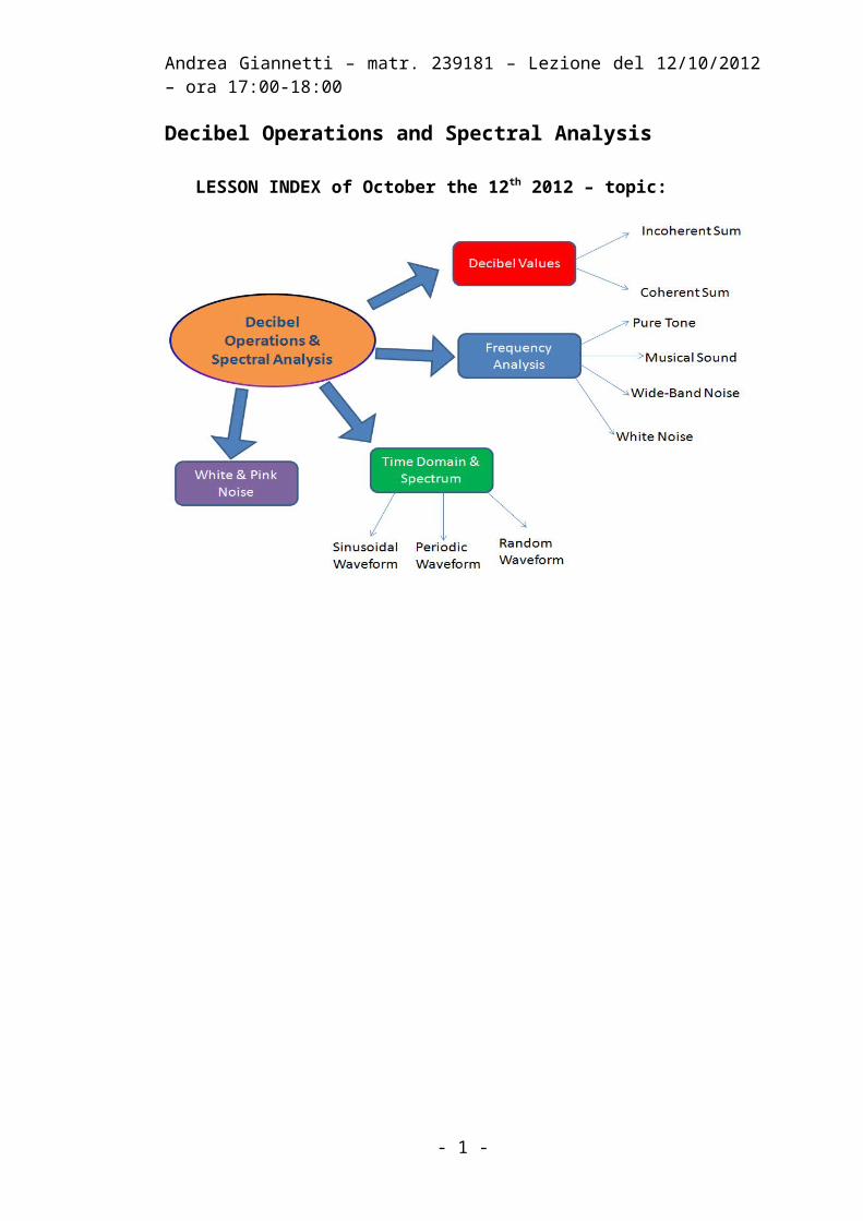
Decibel Operations and Spectral Analysis

LESSON INDEX of October the 12th 2012 – topic:

- 1 -

Lezione del 12/10/2012 – 17:00-18:00

Decibel values: sum and difference

Decibels, are not units on which we could operate as of kilograms and meters, in fact if we take two decibels, it doesn’t mean take twice a decibel.

We need to perform basic mathematical operations (sum and difference) to properly use these parameters.

“Incoherent” (energetic) sum of two “different” sounds:

It is, for example, two sound sources that emit a certain sound pressure level (different from each other); when a source emits a sound of 80 dB, and the other emits a sound of 85 dB, what is the value in dB of the overall sound, which is the sum of the two?

Of course, it’s not the algebraic sum of the two, 80+85 doesn’t mean 165 dB, because Decibels are logarithmic quantities.

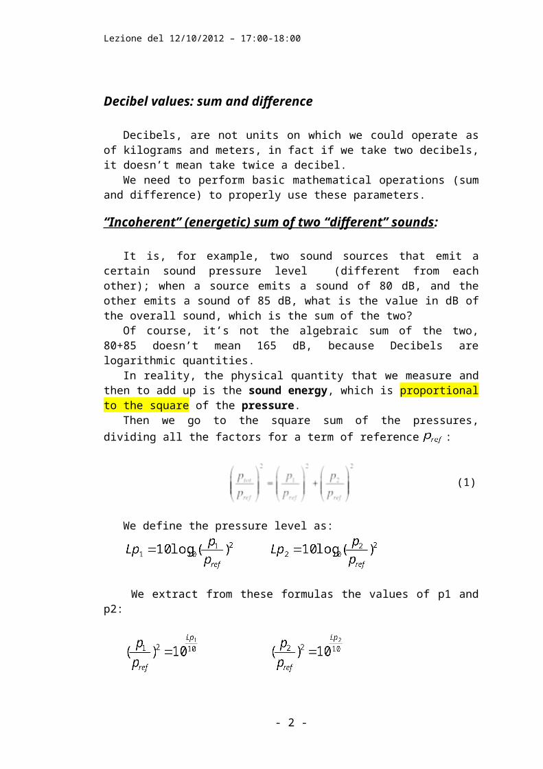
In reality, the physical quantity that we measure and then to add up is the sound energy, which is proportional to the square of the pressure.

Then we go to the square sum of the pressures, dividing all the factors for a term of reference :

(1)

We define the pressure level as:

We extract from these formulas the values of p1 and p2:

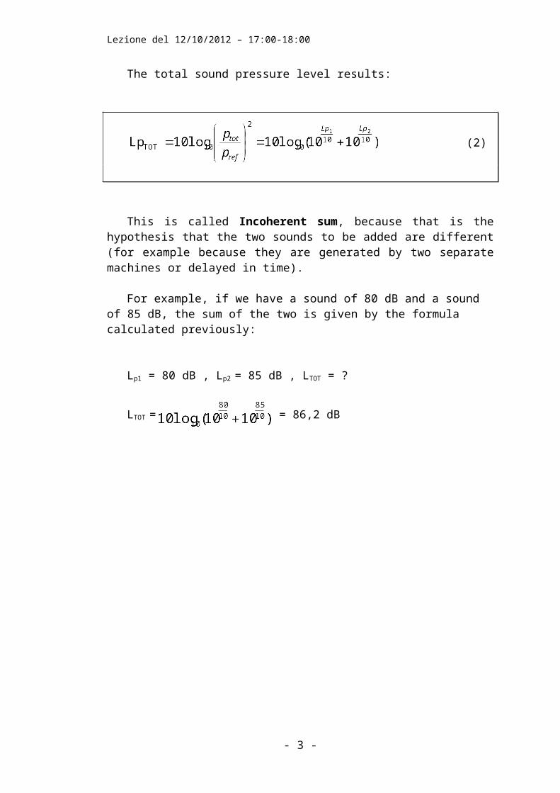
The total sound pressure level results:

(2)

This is called Incoherent sum, because that is the hypothesis that the two sounds to be added are different (for example because they are generated by two separate machines or delayed in time).

- 2 -

Lezione del 12/10/2012 – 17:00-18:00

For example, if we have a sound of 80 dB and a sound of 85 dB, the sum of the two is given by the formula calculated previously:

Lp1 = 80 dB , Lp2 = 85 dB , LTOT = ?

LTOT = = 86,2 dB

0

0.2

0.4

0.6

0.8

1

1.2

1.4

1.6

1.8

2

2.2

2.4

2.6

2.8

3

0 1 2 3 4 5 6 7 8 9 10

difference between the two levels in dB

corre

ctio

n to

add

to th

e lar

ger l

evel

Figure 1: Graph in which the abscissa shows the difference between the two levels, while on the ordinate the amount to be added to the higher level

Just as before, if we have to make a subtraction:

Lp1 = 80 dB , Lp2 = ?, LTOT = 85 dB

Lp2 = = 83,35 dB

If we have two signals with the same level of pressure and let them to add up, the level of total pressure will be increased by 3 dB; this is a general rule.

If we have two signals which differ by 10 dB or more, then their sum will be equal to the larger of the two.

- 3 -

Lezione del 12/10/2012 – 17:00-18:00

For example Lp1 = 90 dB Lp2 = 80 dB LTOT = 90 dB

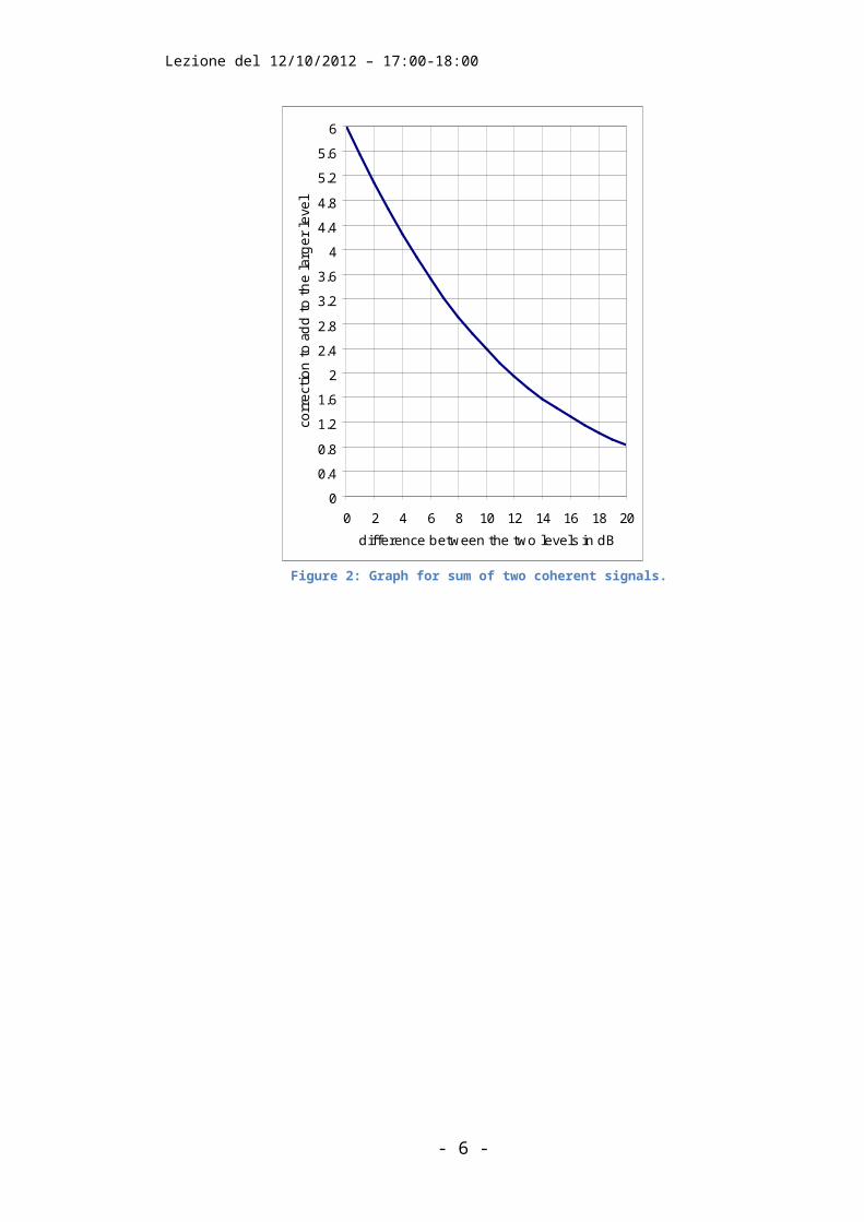
There is also the case of coherent sum between two signals, which is applied in the case in which the two signals are identical to each other; in this case the instantaneous values of sound pressure are going to sum.

But, as at any instant the two waveforms are identical, even after RMS time averaging we get that the average total RMS pressure is given by the sum of the two RMS averaged original pressures. Hence we have:

(3)

0

0.4

0.8

1.2

1.6

2

2.4

2.8

3.2

3.6

4

4.4

4.8

5.2

5.6

6

0 2 4 6 8 10 12 14 16 18 20

difference between the two levels in dB

corre

ctio

n to

add

to th

e lar

ger l

evel

Figure 2: Graph for sum of two coherent signals.

- 4 -

Lezione del 12/10/2012 – 17:00-18:00

- 5 -

Lezione del 12/10/2012 – 17:00-18:00

Frequency Analysis - Spectrum

Frequency Analysis means to obtain the spectrum of a signal; but what is a spectrum?

A spectrum of a signal is a chart that has the frequencies on the abscissa, while as ordinates the sound pressure level in dB; simple tones have spectra composed by just a small number of “spectral lines”, whilst complex sounds usually have a “continuous spectrum”.

Now we will consider the spectra of four very basic cases:

a) Pure tone: this is a purely sinusoidal waveform, the corresponding spectrum presents only one vertical line because this tone has energy at only one single frequency, while all the others are null (just as the sound of a diapason).

Figure 3: Spectrum of a pure tone.

b) Musical sound: these types of sounds, are characterized by a "harmonic comb", that is a discrete number of pure tones normally placed at integer multiples of the “fundamental” frequency. The first frequency is called the fundamental frequency and gives the pitch of the note.There are also so-called inharmonic sounds, which have frequencies that are not integer multiples of the fundamental.

Figure 4: Spectrum of a musical sound.

c) Wide-band noise: these types of sound, have a continuous spectrum, in fact there is always energy at every frequency, loud or weak. These spectra are typical of noise sources.

- 6 -

Lezione del 12/10/2012 – 17:00-18:00

Figure 5: Spectrum of a Wide-band noise.

d) “White noise”: the white noise is a particular type of noise that has the same energy level at all frequencies (a flat line); typically it is generated artificially, for example by a computer, an example of natural white noise is the compressed air coming out from a cylinder.

Figure 6: Spectrum of white noise.

Time-domain waveform and spectrum

There is a relationship between the wave shape in the time domain (like the one shown by the oscilloscope) and the spectrum of the sound.

a) Sinusoidal waveform: A sinusoidal waveform translates into a pure tone. The vertical line is set at the fundamental frequency, which is the reciprocal of the period in the time domain.

Figure 7: Sinusoidal waveform (time domain) and its spectrum.

- 7 -

Lezione del 12/10/2012 – 17:00-18:00

b) Periodic waveform: A periodic waveform translates into a musical sound. The period is given by the fundamental frequency of the spectrum.

Figure 8: Periodic waveform (time domain) and its spectrum.

c) Random waveform: A random sequency of number, a completely random distribution values. This is typically of noise, and the spectrum has energy ad every frequency.

Figure 9: Random waveform (time domain) and its spectrum.

There are two different methods to build the spectrum of a signal, in fact there are two types of filter banks that are commonly employed for frequency analysis:

• constant bandwidth (FFT);• constant percentage bandwidth (1/1 or 1/3 of octave).

The second approach is better than the first one.

The first one is almost always implemented by an algorithm called FFT which means Fast Fourier Transform, but it relies on hypotheses that are usually not met in acoustic.

The FFT provides for the division of the band of frequencies in many narrow segments, equal to each others, of predefined length. The algorithm usually is applied to a digitally-sampled signal, of which a short segment is taken, with a length (in samples) that is equal to a multiple of 2 (1024, 2048, 4096 samples, etc.) because in this way the calculation of the spectrum is very rapid.

- 8 -

Lezione del 12/10/2012 – 17:00-18:00

The second one provides for the division of the frequency band into many segments different from each other: in case of octave band, each band has a width which is double of the previous (1 2 4...).We label each band after its center frequency, defined as the geometric mean value between the upper and lower extremes of the band analyzed:

(4)

For example the octave band of 1 kHz goes from 707 Hz to 1414 Hz, with a central frequency of 1000 Hz. This is also called the Central Octave.

An Octave band spans from a frequency to its double:

(5)

Instead if we use 1/3 octave band analysis, each octave is further divided by 3, so the ratio between the upper frequency and the lower frequency of each band results:

(6)

This is quite close to “human resolution”.

Figure 10: Reference frequency for octave band and 1/3 octave band.

- 9 -

Lezione del 12/10/2012 – 17:00-18:00

White noise and pink noise

White noise is flat in narrowband analysis (FFT) because at every 1 Hz band it takes the same sound pressure level.

However, if we look at the white noise in 1/3 octave bands, it is no longer flat, because every band is becoming larger, in fact every octave band is twice than the previous one, so it gets twice energy, that means 3 dB more every octave.

Figure 11: Spectrum of the White Noise in Narrowband (flat) and in 1/3 octave (growing 3 dB for octave).

The pink noise is a is a type of noise that is flat in the 1/3 octave; and this of course means that it will not be flat in narrowband, but will be decreasing by 3 dB per octave.

Figure 12: Spectrum of the Pink Noise in 1/3 octave(flat) and in Narrowband (decreasing 3 dB for octave).

Pink noise is the most widely used noise in acoustics, while white noise is not a good test source, because it has a lot of energy at high frequency.

Critical bands (BARK)The human auditory system, operates in bands called BARK (critical

bands); these bands are 24, as we see in the next figure.

- 10 -

Lezione del 12/10/2012 – 17:00-18:00

At medium and high frequencies, the width of the BARK bands and the 1/3 octave bands are comparable.

At low frequencies, the critical bands remain very large (100 Hz), while those of 1/3 octave band are very narrow.

Figure 13: Bark bands (left) and 1/3 octave bands (right) analyzing the various frequencies.

Confronto ampiezze di banda - Bark vs. 1/3 Octave

1

10

100

1000

10000

10 100 1000 10000

Frequenza (Hz)

Ban

dwid

th (H

z)

BarkTerzi

Figure 14: Comparison between bark bands and 1/3 octave bands.

- 11 -