ESCUELA TÉCNICA SUPERIOR DE INGENIERÍA (ICAI ...Analysis of Variance –ANOVA- will be done. In...

ESCUELA TÉCNICA SUPERIOR DE INGENIERÍA

(ICAI)

GRADO EN INGENIERÍA ELECTROMECÁNICA

EXPERIMENTAL INVESTIGATION OF

VITAL PROCESS PARAMETERS ON

RECAST LAYER THICKNESS

Autor: Javier Angoloti Gálvez

Director: Paul Xirouchakis

Assistants: Dr Ahmed Bufardi, Olcay Atken, Dr Kiran Gopalakrishna

Bhat

Madrid

Julio 2015

AUTORIZACIÓN PARA LA DIGITALIZACIÓN, DEPÓSITO Y DIVULGACIÓN EN ACCESO

ABIERTO ( RESTRINGIDO) DE DOCUMENTACIÓN

1º. Declaración de la autoría y acreditación de la misma.

El autor D. Javier Angoloti Gálvez , como alumno de la UNIVERSIDAD PONTIFICIA COMILLAS

(COMILLAS), DECLARA

que es el titular de los derechos de propiedad intelectual, objeto de la presente cesión, en relación

con la obra Proyecto Fin de Grado: Experimental investigation of vital process parameters on recast

layer thickness, que ésta es una obra original, y que ostenta la condición de autor en el sentido que

otorga la Ley de Propiedad Intelectual como titular único o cotitular de la obra.

En caso de ser cotitular, el autor (firmante) declara asimismo que cuenta con el consentimiento de

los restantes titulares para hacer la presente cesión. En caso de previa cesión a terceros de

derechos de explotación de la obra, el autor declara que tiene la oportuna autorización de dichos

titulares de derechos a los fines de esta cesión o bien que retiene la facultad de ceder estos

derechos en la forma prevista en la presente cesión y así lo acredita.

2º. Objeto y fines de la cesión.

Con el fin de dar la máxima difusión a la obra citada a través del Repositorio institucional de la

Universidad y hacer posible su utilización de forma libre y gratuita ( con las limitaciones que más

adelante se detallan) por todos los usuarios del repositorio y del portal e-ciencia, el autor CEDE a

la Universidad Pontificia Comillas de forma gratuita y no exclusiva, por el máximo plazo legal y con

ámbito universal, los derechos de digitalización, de archivo, de reproducción, de distribución, de

comunicación pública, incluido el derecho de puesta a disposición electrónica, tal y como se

describen en la Ley de Propiedad Intelectual. El derecho de transformación se cede a los únicos

efectos de lo dispuesto en la letra (a) del apartado siguiente.

3º. Condiciones de la cesión.

Sin perjuicio de la titularidad de la obra, que sigue correspondiendo a su autor, la cesión de

derechos contemplada en esta licencia, el repositorio institucional podrá:

(a) Transformarla para adaptarla a cualquier tecnología susceptible de incorporarla a internet;

realizar adaptaciones para hacer posible la utilización de la obra en formatos electrónicos,

así

como incorporar metadatos para realizar el registro de la obra e incorporar “marcas de agua” o

cualquier otro sistema de seguridad o de protección.

(b) Reproducirla en un soporte digital para su incorporación a una base de datos electrónica,

incluyendo el derecho de reproducir y almacenar la obra en servidores, a los efectos de garantizar

su seguridad, conservación y preservar el formato. .

(c) Comunicarla y ponerla a disposición del público a través de un archivo abierto institucional,

accesible de modo libre y gratuito a través de internet.1

(d) Distribuir copias electrónicas de la obra a los usuarios en un soporte digital. 2

4º. Derechos del autor.

El autor, en tanto que titular de una obra que cede con carácter no exclusivo a la Universidad por

medio de su registro en el Repositorio Institucional tiene derecho a:

a) A que la Universidad identifique claramente su nombre como el autor o propietario de los

derechos del documento.

b) Comunicar y dar publicidad a la obra en la versión que ceda y en otras posteriores a través de

cualquier medio.

c) Solicitar la retirada de la obra del repositorio por causa justificada. A tal fin deberá ponerse en

contacto con el vicerrector/a de investigación ([email protected]).

d) Autorizar expresamente a COMILLAS para, en su caso, realizar los trámites necesarios para la

obtención del ISBN.

1 En el supuesto de que el autor opte por el acceso restringido, este apartado quedaría redactado en los

siguientes términos:

(c) Comunicarla y ponerla a disposición del público a través de un archivo institucional, accesible de modo

restringido, en los términos previstos en el Reglamento del Repositorio Institucional

2 En el supuesto de que el autor opte por el acceso restringido, este apartado quedaría eliminado.

d) Recibir notificación fehaciente de cualquier reclamación que puedan formular terceras personas

en relación con la obra y, en particular, de reclamaciones relativas a los derechos de propiedad

intelectual sobre ella.

5º. Deberes del autor.

El autor se compromete a:

a) Garantizar que el compromiso que adquiere mediante el presente escrito no infringe ningún

derecho de terceros, ya sean de propiedad industrial, intelectual o cualquier otro.

b) Garantizar que el contenido de las obras no atenta contra los derechos al honor, a la intimidad y

a la imagen de terceros.

c) Asumir toda reclamación o responsabilidad, incluyendo las indemnizaciones por daños, que

pudieran ejercitarse contra la Universidad por terceros que vieran infringidos sus derechos e

intereses a causa de la cesión.

d) Asumir la responsabilidad en el caso de que las instituciones fueran condenadas por infracción

de derechos derivada de las obras objeto de la cesión.

6º. Fines y funcionamiento del Repositorio Institucional.

La obra se pondrá a disposición de los usuarios para que hagan de ella un uso justo y respetuoso

con los derechos del autor, según lo permitido por la legislación aplicable, y con fines de estudio,

investigación, o cualquier otro fin lícito. Con dicha finalidad, la Universidad asume los siguientes

deberes y se reserva las siguientes facultades:

a) Deberes del repositorio Institucional:

- La Universidad informará a los usuarios del archivo sobre los usos permitidos, y no garantiza ni

asume responsabilidad alguna por otras formas en que los usuarios hagan un uso posterior de las

obras no conforme con la legislación vigente. El uso posterior, más allá de la copia privada,

requerirá que se cite la fuente y se reconozca la autoría, que no se obtenga beneficio comercial, y

que no se realicen obras derivadas.

- La Universidad no revisará el contenido de las obras, que en todo caso permanecerá bajo la

responsabilidad exclusiva del autor y no estará obligada a ejercitar acciones legales en nombre del

autor en el supuesto de infracciones a derechos de propiedad intelectual derivados del depósito y

archivo de las obras. El autor renuncia a cualquier reclamación frente a la Universidad por las

formas no ajustadas a la legislación vigente en que los usuarios hagan uso de las obras.

- La Universidad adoptará las medidas necesarias para la preservación de la obra en un futuro.

b) Derechos que se reserva el Repositorio institucional respecto de las obras en él registradas:

- retirar la obra, previa notificación al autor, en supuestos suficientemente justificados, o en caso

de reclamaciones de terceros.

Madrid, a ……….. de …………………………... de ……….

ACEPTA

Fdo……………………………………………………………

Proyecto realizado por el alumno/a:

Javier Angoloti Gálvez

Fdo.: …………………… Fecha:

Autorizada la entrega del proyecto cuya información no es de carácter confidencial

EL DIRECTOR DEL PROYECTO

Paul Xirouchakis

Fdo.: …………………… Fecha:

Vº Bº del Coordinador de Proyectos

Jesús Ramón Jiménez Octavio

Fdo.: …………………… Fecha:

Summary of the project Experimental investigation of vital process parameters on recast layer thickness The final objective of the project Experimental investigation of vital process parameters

on recast layer thickness is to help find data for the project Intelligent Fault Correction

and self-Optimizing Manufacturing system, IFaCOM; which seeks to achieve near zero

defect levels in manufacturing. Moreover, the former project is centered in wire

electrical discharge machining –or WEDM- and a manufacturing characteristic known

as the recast layer or white layer. The latter project is a collaboration between

universities; including the Norwegian University of Science and Technology-NTNU

and the École Polytechnique Fédérale de Lausanne-EPFL amongst others and

companies such as Agie Charmilles (where the stainless steel samples for the first

project were achieved) and GKN Aerospace.

Wire electrical discharge machining is a non-traditional manufacturing method, used

due to its high precision and ability to cut high strength steels. It is used mainly in the

manufacturing of dies and prototypes; and is buoyant in the aerospace industry. In

this process, an electrical current passes through a brass wire and is refrigerated by

means of de-ionized water or cooling oil. The wire then will be used to cut an

electrically conductive workpiece, due to the high heat sparks created between the

wire and the workpiece.

The recast layer is a brittle layer created due to the high heat that the workpiece is

affected by during the WEDM process; it is related too to the final quality of the

workpiece (the smaller the recast layer is, the better the final workpiece will be). In

the following figure the recast layer can be appreciated, thanks to a micrograph at

500x:

The roughness will too be studied, and lastly a brief chemical composition analysis

will be discussed. Roughness is also a quality parameter ubiquitous in the

manufacturing industry.

Recast layer thickness, roughness and chemical composition are the outputted

qualities measured. As for the inputted parameters studied, they will be the following:

Voltage, Pulse off time and Feed-rate. The Voltage is the fed electrical tension of the

wire –also known as gap voltage- Pulse off time is the time in which there is no

electrical tension in the pair wire-workpiece (i.e. when there is no spark between

workpiece and wire) and Feed-rate is the speed at which the workpiece is cut.

35 different combinations of Voltage, Pulse off time and Feed-rate will give the

opportunity of studying the outputs of recast layer thickness and roughness. Each

sample had to be prepared for being able to measure the recast layer thickness,

roughness and chemical composition.

For the preparation of the recast layer thickness and chemical composition samples,

the base samples had to be embedded in a resin, polished and chemically attacked.

With these prepared samples, micrographs were taken to measure the thickness, and

each sample had at least eight thickness measurements, which were then averaged.

These measurements could be done thanks to a data acquisition software that

permitted the dimensioning of the workpiece. The chemical composition

measurement was very time consuming, and could only be done in three different

samples; as the resin was non-conductive and said measurements were done thanks

to spectroscopies –which need of electrically conductive materials (such as the base

steel of the samples). Therefore the chemical composition was studied to qualitatively

find if molten brass was deposited in the workpiece.

As for the roughness of the finished workpiece, it could not be measured with the

same samples as the ones aforementioned, as they were embedded in resin and then

polished. Hence, new samples were prepared, without the need of embedding. To

measure the roughness, a perthometer was used.

To study how much each inputted parameter affects the quality parameters, an

Analysis of Variance –ANOVA- will be done. In this analysis, a significance level α will

be fixed at 5%, then the p-value will be studied between inputted parameters and the

quality parameters. If said p-value is smaller than α, then it can be derived that the

quality parameter is affected by one of the machining parameters.

After the ANOVA is finished, multiple comparison graphs will be used to have a more

visual interpretation of the results derived by the ANOVA. An example of a multiple

comparisons graph follows:

This graph will compare the different inputted Voltages with the measured surface

roughness. In blue are the surface roughnesses measured for each voltage, with the

notch being the mean. In this case, the ANOVA gave p-value≈0 implying the surface

will vary strongly with different voltages. According to the measurements, said

statement is true and can be seen graphically in the aforementioned multiple

comparisons graph: at bigger voltage, bigger roughness.

At last, the correlation between recast layer thickness and roughness was studied. The

motivation of this study was to qualitatively find if roughness and recast layer

thickness were dependent, as it can be seen in the first figure, intuition tells that

maybe at bigger recast layer thickness, stronger surface roughness.

As for the main conclusions derived:

Voltage will affect the recast layer thickness

Voltage and Pulse off time affect the roughness

The chemical composition analysis qualitatively found that there is brass

deposited in the surface of the workpiece

Roughness and recast layer thickness are independent

Resumen del proyecto Experimental investigation of vital process parameters on recast layer thickness El objectivo final del proyecto Experimental investigation of vital process parameters

on recast layer thickness es de suministrar datos para el proyecto Intelligent Fault

Correction and self-Optimizing Manufacturing system, IFaCOM; que busca encontrar un

nivel mínimo de defectos en la mayor parte de técnicas de fabricación. Este primer

proyecto se centra en electroerosión por hilo –WEDM por sus siglas en inglés- y una

característica de calidad conocida como recast layer. En el segundo proyecto,

universidades colaboran con compañías para encontrar este nivel mínimo de defectos.

Universidades relacionadas con el proyecto son la Norwegian University of Science

and Technology-NTNU y la École Polytechnique Fédérale de Lausanne-EPFL entre

otras; también colaboran compañías como Agie Charmilles (de donde las muestras de

acero inoxidable se consiguieron) y GKN Aerospace.

La electroerosión por hilo es una técnica de fabricación no tradicional, usada por su

buena precisión y habilidad de corte, en especial en aceros rápidos (HSS). Esta técnica

es usada en la fabricación de moldes y prototipos, y su uso es cada vez más popular en

la industria aeroespacial. Durante el proceso, una tensión eléctrica alimenta un hilo de

latón que es refrigerado por agua desionizada o líquido refrigerante. El hilo, al

contactar eléctricamente con la pieza –que también debe conducir la electricidad-

hará saltar una chispa a muy alta temperatura, con la que se cortará la pieza.

La recast layer es una capa frágil y dura que es creada por las altas temperaturas

alcanzadas por el hilo de latón durante el proceso de WEDM. El espesor de esta capa

está relacionado con la calidad de la pieza (a menor espesor, mejor calidad de dicha

pieza). En la próxima imagen (hecha a 500 aumentos) se puede ver la capa, también

llamada en la literatura inglesa white layer:

Siendo base steel el acero base, recast layer la capa mencionada antes y brass

deposition el latón del hilo que se funde durante el proceso de WEDM.

La rugosidad también se estudiará, al igual que se hará un corto análisis de la

composición química. La rugosidad es un parámetro de calidad más tradicional que el

espesor de la recast layer, y es usada en otros ámbitos de fabricación.

Los parámetros medidos en el proyecto han sido el espesor de la recast layer, la

rugosidad y la composición química. Los parámetros implementados para las

diferentes muestras son: Voltaje, Pulse off time y Velocidad de avance. El Voltaje es la

tensión eléctrica del hilo, el Pulse off time es el tiempo cuando no existe tensión en el

par hilo-pieza (o séase cuando no hay chispa entre hilo y pieza) y la Velocidad de

avance es la velocidad con la que el hilo avanza para cortar la pieza.

Son 35 las diferentes combinaciones entre Voltaje, Pulse off time y Velocidad de

avance que se han estudiado para medir ambos parámetros de calidad. Cada muestra

ha tenido que ser preparada adecuadamente para medir dichos parámetros.

Para la preparación de las muestras en las que se miden espesores y composiciones

químicas, éstas tuvieron que ser curadas en una resina, pulidas y luego atacadas

químicamente. Con dichas muestras y la ayuda de un microscopio óptico con un

software de adquisición de imágenes se pudieron medir los espesores –al menos ocho

espesores de la recast layer se hicieron por muestra y luego fueron promediados. El

análisis químico requirió mucho tiempo, al usarse una resina no conductiva y usarse

espectroscopias –que necesitan de materiales conductivos (como el acero de la pieza

base). Esto es, el análisis químico se usó para demostrar cualitativamente si había

deposición de latón en la recast layer y se hizo solamente en tres diferentes muestras.

Respecto a la rugosidad de la pieza, no pudo ser medida con las mismas muestras

usadas para la medición de los espesores, al estar estas cubiertas en resina y además

pulidas. Entonces, nuevas muestras tuvieron que ser preparadas exclusivamente para

la medición de la rugosidad (para ello se utilizó un rugosímetro).

Para estudiar cómo cada parámetro de fabricación afecta a cada parámetro de calidad

un estudio Análisis de la Varianza –ANOVA- fue hecho. En dicho análisis, un nivel de

significación α es fijado al 5%, luego el p-valor es estudiado entre los parámetros de

fabricación y aquellos de calidad. Si p-valor< α se puede decir que el parámetro de

calidad es afectado por uno de los parámetros de fabricación.

Después de hacer el ANOVA, diagramas simples de cajas y patillas (llamados multiple

comparisons graphs en inglés) han sido usados para dar una interpretación más visual.

Un ejemplo de este diagrama puede verse:

Donde se comparan Voltaje y rugosidad medida. En azul están las medidas de

rugosidad para cada voltaje, siendo el punto central la media. En este caso en

particular, la ANOVA dio un p-valor≈0, que implica que la rugosidad varía fuertemente

con el voltaje. Según estas mediciones y el diagrama de cajas y patillas ambas

herramientas estadísticas se complementan y concluyen que a mayor voltaje, mayor

rugosidad.

Por último, se estudió la correlación entre el espesor de la recast layer y la rugosidad.

La motivación de este estudio es la de encontrar si ambos parámetros son

dependientes, al poderse ver en la primera imagen, se puede empezar suponiendo que

a mayor espesor de la capa, mayor rugosidad.

En cuanto a las conclusiones principales:

El Voltaje afecta el espesor de la recast layer

El Voltaje y Pulse off time afectan la rugosidad

El análisis químico encuentra latón fundido en la capa

La rugosidad y recast layer son independientes

ESCUELA TÉCNICA SUPERIOR DE INGENIERÍA

(ICAI)

GRADO EN INGENIERÍA ELECTROMECÁNICA

EXPERIMENTAL INVESTIGATION OF

VITAL PROCESS PARAMETERS ON

RECAST LAYER THICKNESS

Autor: Javier Angoloti Gálvez

Director: Paul Xirouchakis

Assistants: Dr Ahmed Bufardi, Olcay Atken, Dr Kiran Gopalakrishna

Bhat

Madrid

Julio 2015

Experimental investigation of vital process parameters on recast layer thickness

1 Javier Angoloti Gálvez



Motivation

This project is part of the project Intelligent Fault Correction and self-Optimizing

Manufacturing system, IFaCOM, whose goal is to develop methods to achieve close

to zero defect levels in manufacturing processes. IFaCOM will count with three

automation loops: a real time parameter control loop, a process optimization loop

and a machine system optimization loop. A schematic flow graph explaining the

structure of the IFaCOM project can be seen in Figure 1.

Figure 1. Structure of the IFaCOM project1

The paper centers in the process of wire electric discharge machining (WEDM) –

which is a complex machining system that can involve up to 25 machining

parameters. Driving characteristics of WEDM considered in IFaCOM are the recast

layer and roughness of finished pieces. The company collaborating with IFaCOM in

the WEDM process –and where the samples were obtained from- is Agie

Charmilles.

The paper will center on three of the main vital input parameters in this

technology: Voltage, Pulse off time and Feed-rate. The thickness, roughness and

composition of the recast layer will be studied. Afterwards, statistical analysis tools

will be used to relate the input parameters with the finished workpiece

characteristics.

1 (2015) IFaCOM Framework IFaCOM, Norwegian University of Science and Technology, NTNU



Table of contents

Introduction ........................................................................................................................................... 8

Fuzzy logic approach ...................................................................................................................... 8

WEDM functioning .......................................................................................................................... 8

Mechanism of the recast layer’s development ..................................................................... 9

Driving parameters of the formation of the recast layer ...............................................10

Units used .....................................................................................................................................10

Voltage ...........................................................................................................................................10

Pulse off time ..............................................................................................................................10

Feed-rate ......................................................................................................................................11

Experimental procedure .................................................................................................................12

Preparation of the samples ........................................................................................................12

Recast layer thickness and spectroscopy samples .......................................................13

Roughness samples ..................................................................................................................13

Measurement of the recast layer thickness .........................................................................14

Measurement of the roughness ...............................................................................................16

Measurement of the sample’s composition .........................................................................16

Experimental outcomes...................................................................................................................20

Training data ...................................................................................................................................20

Test data ............................................................................................................................................21

Metallurgy results .........................................................................................................................21

Weight percentage composition of the recast layer ....................................................21

Elemental map of recast layer in sample 13 ...................................................................22

Statistical analysis .............................................................................................................................24

ANOVA model .................................................................................................................................24

Regression analysis ......................................................................................................................26

Arithmetic mean and standard deviation ............................................................................26

Results and discussion of the statistical analysis ..................................................................27

ANOVA of recast layer thickness and roughness ..............................................................27

Average recast layer thickness ............................................................................................27

Recalculated average recast layer thickness ..................................................................29

Roughness ....................................................................................................................................29



Contrasting results derived from ANOVA .......................................................................31

Regression analysis ......................................................................................................................31

Roughness and recast layer thickness ..............................................................................31

Roughness and new recast layer thickness ....................................................................32

Chemical composition .................................................................................................................33

Composition of the recast layer in sample 13 ................................................................33



Composition of the roughing recast layer in sample 22 ............................................34

Comparison of compositions of the samples ..........................................................................34

Main conclusions ................................................................................................................................36

Average recast layer thickness .................................................................................................36

Roughness ........................................................................................................................................36

Chemical composition .................................................................................................................36

References ............................................................................................................................................38

Annexes .................................................................................................................................................40

Annex I. Example of the MATLAB code used for the ANOVA .......................................40

Annex II. Measured recast layer thickness samples ........................................................40

Annex II. Electronic micrographs for the spectroscopy .................................................57

List of figures

Figure 1. Structure of the IFaCOM project ................................................................................. 2

Figure 2. Functioning of a WEDM machine [3]......................................................................... 9

Figure 3. Heat affected layers of a workpiece ........................................................................... 9

Figure 4. Pulse off time definition in WEDM [5] ....................................................................10

Figure 5. Micrograph of sample 25 .............................................................................................13

Figure 6. Micrograph of sample 10, including measurements of the recast layer

thickness................................................................................................................................................14

Figure 7. Recalculation of the recast layer thickness example.........................................15

Figure 8. Electron image of the recast layer of sample 13 .................................................17

Figure 9. Spectroscopy example ..................................................................................................17

Figure 10. Elemental map of the recast layer in sample 13 ..............................................22

Figure 11. Comparison of the Feed-rate with the average thickness ............................27



Figure 12. Comparison of the Pulse off time with the average thickness ....................28

Figure 13. Comparison of the Voltage with the average thickness ................................28

Figure 14. Comparison of the Feed-rate with the surface roughness ...........................30

Figure 15. Comparison of the Pulse off time with the surface roughness ...................30

Figure 16. Comparison of the Voltage with the surface roughness ................................30

Figure 17. Regression analysis between roughness and recast layer thickness .......32

Figure 18. Regression analysis between roughness and new recast layer thickness

...................................................................................................................................................................32

Figure 19. Micrograph of the roughing recast layer with a “line” in sample 26 ........35

List of tables

Table 1. Units used ............................................................................................................................10

Table 2. Weight percentage composition of the brass wire ..............................................12

Table 3. Weight percentage composition of Böhler stainless steels ..............................12

Table 4. Experimental outcomes for the training data ........................................................20

Table 5. Test data ...............................................................................................................................21

Table 6. Composition of the recast layer of sample 13 .......................................................21



Table 9. Composition of the recast layer of the roughing surface in sample 22 .......22

Table 10. ANOVA of the thickness of recast layer .................................................................27

Table 11. ANOVA of the new recast layer thickness calculated .......................................29

Table 12. ANOVA of the roughness .............................................................................................29

Table 13. Mean and standard deviation of the composition in sample 13 ..................33



Table 16. Mean and standard deviation of the composition in sample 22, rough ....34

Table 17. Comparison of the composition of the recast layer of samples studied ...34



Introduction

Wire electrical discharge machining (WEDM) is a non-traditional manufacturing

method. It was popularized in the 1960s, for machining high strength steel (HSS)

dies, as well as to manufacture prototypes with experimental materials. Nowadays

it is a popular means of manufacturing pieces that require high precision and need

low residual stresses. Nevertheless, this precision depends on many parameters,

and is highly driven by the recast layer thickness and roughness.

The study of the recast layer’s thickness, surface roughness and composition of

stainless steel samples during this project will be later compared to the prediction

made by an algorithm to correct this recast layer in real-time. The samples will be

prepared varying three input parameters: Voltage, Pulse off time and Feed-rate.

Said algorithm uses a fuzzy-nets approach to finally be incorporated to the WEDM

machine and minimize the layer’s thickness and roughness (in other words, to

minimize the defects). The ultimate goal of the algorithm will be to predict when

will there be a machining defect, changing then the parameters to avoid it [1].

Fuzzy logic approach Fuzzy networks are especially appropriate to approach this prediction, as they are

able to predict non-linear behavior and imprecision without the use of differential

equations (they model processes without a mathematical model or with strong

non-linearities). Fuzzy logic is not a true/false logic such as classical logic, but

accepts a range of states between true and false. It is said it approximates the

reasoning to that of a human [1].

In IFaCOM, fuzzy-nets are used to predict the values of Vital Quality Characteristics

–recast layer thickness and roughness- by implementing and adjusting Vital

Process Parameters –Feedrate, Voltage and Pulse off time. In this project, the latter

are experimentally measured and then compared to the former to complete results

in the fuzzy networks prediction algorithm. The measurements will also be used to

validate said algorithm.

WEDM functioning To cut a workpiece with WEDM, an electrical current passes through a wire

(generally made of brass or copper), which is constantly moving and is supplied by

reels –both wire and workpiece shall be electrically conductive. This will create a

spark powerful enough to cut through high strength materials such as HSS.

Note how in Figure 2 the wire does not touch the piece to be machined, leaving a

spark gap. The spark will heat the piece and wire, thus de-ionized water will be

used to cool off both during the process; it is due to this heating that the recast

layer appears [2]. The wire’s path will be controlled by a CNC machine in the x-y



plane. Some machines allow for vertical tapers allowing the movement in the z

direction.

Figure 2. Functioning of a WEDM machine [3]

Mechanism of the recast layer’s development It is the high temperature achieved by the spark and the corrosion by the dielectric

liquid that creates a change of the piece’s properties in the machined surface. This

change of physical properties shall be reduced; as it not only makes said surface

more brittle, but it can temper the original piece up to a depth of 50µm (the HAZ in

Figure 3), making that part softer. The change on the crystallographic structure –

due to the heat- of the base workpiece is responsible for these changes, creating

the HAZ and the recast layer or white layer.

The recast layer will have a roughness that is usually not desired, and needs of

more passes of the wire, up to 4 –although it can lead to undesired residual strain

and a more costly process [4].

A detailed zone of the white recast layer can be seen in Figure 6, where a finished

sample has been studied under an optical microscope.

Figure 3. Heat affected layers of a workpiece



Driving parameters of the formation of the recast

layer As discussed earlier, the driving parameters studied in this report will be Voltage,

Pulse off time and Feed-rate.

Units used In Table 1 the units used during the tests and throughout the paper are

summarized.

Parameter Unit Symbol Voltage Volts [V]

Pulse off time Milliseconds [ms] Feed-rate Millimeters per minute [mm/min]

Table 1. Units used

Voltage The voltage U specified for each specimen is that of the electric tension supply of

the brass wire. It is denominated by the gap voltage, U0, specified in Figure 4.

Pulse off time Pulse off time is a parameter exclusive to EDM and WEDM, not found in any other

machining methods.

The pulse off time, represented as to in Figure 4, is the time between the discharge

voltage Ue –between wire and piece- and the gap voltage Uo –the voltage of the

brass wire before interacting with the workpiece. The ignition delay time td is the

time between the beginning of the pulse of voltage and the spark provoked. During

td and to there is no current between wire and workpiece, hence there is no spark.

The control of this parameter is essential in a good surface finish in EDM and

WEDM processes [5].

Figure 4. Pulse off time definition in WEDM [5]



The machining energy of the WEDM process (valid only during the discharge or

spark time) can be derived as [6]:

While the instantaneous energy or power will be the rate at which this energy is

provided:

Feed-rate The feed-rate is the speed with which the wire advances to machine the desired

workpiece. It is a ubiquitous cutting parameter, of which the finishing surface of a

traditionally machined workpiece (milling, drilling, lathing, etc.) is dependent.

In the case of WEDM, it is studied as being an important parameter that could

influence the quality of the finished piece. It is also an indicative of the speed at

which the pieces will be produced.



Experimental procedure

For collecting the necessary data for the fuzzy-nets algorithm, a set of experiments

were conducted –measurement of the recast layer thickness and roughness.

Moreover, a spectroscopy of three samples was conducted in order to see the

composition of the machined surface, in order to determine if there would be any

deposition of brass from the wire.

A total number of 35 samples -27 used for training data for the fuzzy-nets

algorithm and 8 used as test data- were prepared. Some of the samples were then

not available for all the experiments; this will be specified as N/A in the results.

For the preparation of the samples, a brass wire was used, and two different

stainless steels were used. The composition of the three can be seen in Table 2 and

Table 3:

Cu Zn Brass 63 37

Table 2. Weight percentage composition of the brass wire

Fe C Si Mn Cr W P S Mo V K107 85.05 2.10 0.25 0.4 11.50 0.70 - - - - K110 84.08 1.51 0.32 0.27 11.60 0.02 0.019 0.016 0.63 0.91

Table 3. Weight percentage composition of Böhler stainless steels2

Preparation of the samples In order to be able to measure the roughness and recast layer thickness, as well as

the chemical composition, 35 samples cut with different input parameters were

prepared –refer to Table 4 and Table 5. These 35 samples were used to

measure the recast layer thickness and chemical composition, as they were first

prepared for measuring the recast layer thickness. After preparing these samples,

a new batch of 28 samples were prepared to measure the roughness, as the latter

samples were polished, consequently being biased for the measurement of the

roughness.

In Figure 5, a micrograph of sample 25 in the roughing surface can be used to

explain the measurements of recast layer thickness, chemical composition and

roughness. As seen, the recast layer is not uniform and has defects such as cracks

or pores [5] –as it is very brittle due to its high carbon content, which will influence

negatively in the surface quality and mechanical properties of the workpiece. It is

interesting too to see the golden part, which later will be proved to be the molten

brass wire. This is non-desirable for the final workpiece, as the mechanical

properties of brass are not those of the base metal.

2 (1998) Cold Work Tool Steels. Böhler



Figure 5. Micrograph of sample 25

Recast layer thickness and spectroscopy samples The samples came from a base workpiece and where then cut into rectangular

prisms, with a surface of 7mm*2mm. One of the surfaces of the samples was

finished, with the input parameters implemented; the other was roughed. To make

the distinction between rough and finished surfaces after the embedding, a

micrograph of the roughness was made in each sample.

The first 35 samples were prepared to be polished. In order to polish the samples,

they were embedded into molds with a resin matrix –made by mixing a polymer

powder and a liquid solution (Technovit 40713). After the resin was cured, the

samples were polished using different sandpaper discs –starting with SiC discs of

grits 320 to 1200 and finishing with diamond suspensions of grits 6µm and 1µm.

Lastly they were treated with a chemical attack of NITAL 6% (94% ethanol, 6%

nitric acid; in weight percentages) to distinguish between the interfaces of the

samples under the optical microscope.

Roughness samples To measure the roughness, different samples of stainless steel were prepared. In

each sample, six different combinations of the input parameters were applied,

these being the ones seen in Table 4 and Table 5.

In order to prepare the samples, three wire passes per sample were implemented.

Listed in order of execution:

1. Cutting. For all samples came from a same block of stainless steel, in order

to separate a measurable sample, it should be cut off from said block.

2. Surfacing. Before the passes of finishing, a surfacing of the cut face will

improve the final quality of the piece [7].

3 (2013) Technovit ® Resins, Heraeus Kulzer



3. Finishing. Here, every 8mm of wire feedrate, different parameters were

implemented (for the parameters of each sample, please refer to Table 4

and Table 5). This gives opportunity to measure six different values of

roughness per sample -each sample with a length of 50mm- thus, the last

finishing pass is 10mm long instead of 8mm long as the first five.

This implies one of the surfaces of each sample is roughly finished and the other

will be the one measured.

Measurement of the recast layer thickness After preparing the samples, the surface to be measured was cleaned with ethanol.

Afterwards, said samples were observed under an optic microscope Leica-Leitz

METALLOVERT. Thanks to the data acquisition software (DAQ) and the digital

camera Olympus Colorview SIS, the images could be digitalized. Moreover, the DAQ

also permitted to make on-time measurements of the images, after an appropriate

calibration.

An example of a measurement can be seen in Figure 6, where the dark matrix is the

polymerized resin and the dark part is the original steel (after polishing). The

recast layer is the white interface between the resin and the steel. The majority of

samples were taken with 500x magnification, although 200x and 1000x

magnifications were used in order to describe the samples or to measure thin

recast layers (<1µm), respectively.

Figure 6. Micrograph of sample 10, including measurements of the recast layer thickness



To calculate the overall recast layer thickness, at least eight measurements of said

thickness were executed per sample. Afterwards, the maximum and average of

these measurements were determined.

A new recast layer calculation was also made, following this criterion:

This recalculation was done by approximating the area of the recast layer by

means of rectangles. All in all, it will give a more accurate result of the recast layer

overall thickness than the method aforementioned.

In Figure 7, an example of the recalculation of the recast layer is done. The length

of the micrograph is of approximately 140µm; in blue are rectangles approximated

by the maximum thickness -6.07µm- and in red by the minimum one -1.38µm. The

former will have a length of 80µm and the latter a length of 60µm, thus, the

recalculated thickness will be:

Figure 7. Recalculation of the recast layer thickness example

Note that the local recast layer thickness can be much higher than the average

(refer to Table 4). Note than in Table 4 and Table 5 samples 5, 15 and 34 were not

measurable, because it was impossible to unmold these embedded samples. This is

noted as N/A in said tables.



Measurement of the roughness The prepared samples were covered by a thin layer of rust. Said samples were

therefore cleaned by brushing them with weak NITAL (a solution of nitric acid and

alcohol), which only removed the rust, and did not affect the roughness of the

samples.

To measure the roughness, three passes throughout the width of the sample were

made with a profilometer –for each different surface. The passes were made

perpendicular to the wire’s orientation; the roughness Ra was then calculated by

the profilometer and it is included in Table 4 and Table 5.

Measurement of the sample’s composition Using the samples utilized for measuring the recast layer’s thickness, the

composition of the sample’s recast layers can be determined by means of an

electronic microscope ZEISS Merlin4 and a Data Acquisition Software –INCA.

Difficulty came in measuring said compositions, as the samples were embedded in

a non-conductive resin; but for spectroscopies, better results are achieved with

conductive resins. Nevertheless, the metallographic composition will be measured

in the bulk material (around 1µm of depth) which will allow for more precise

measurements than if the composition was studied directly on the surface.

In order to proceed with the spectroscopy, the embedded sample will be seen through an electronic microscope –as stated before; a conductive resin would provide better results, for instance resin Technovit 50005. With the electronic microscope the area of interest (recast layer) is identified. As seen in Figure 8, the recast layer is the smoother part between the workpiece (in the upper part of the image) and the resin (brighter, in the lower part of the image). The windows in Figure 8 called Spectrum 1 and Spectrum 2 are the zones where the spectroscopy will take place. The brighter parts in the bottom of Figure 8 must not be mistaken by the recast layer (called also white layer), as these parts are out-of-plane with respect to the workpiece, they are part of the resin.

4 (2012) MERLIN Analytical power for the sub-nanometer world, ZEISS Germany 5 (2013) Technovit ® Resins, Heraeus Kulzer



Figure 8. Electron image of the recast layer of sample 13

For the spectroscopy, the sample was charged electrically and then radiated

electromagnetically. In order to find the elements present in a Spectrum window,

one must, in the software, specify the alloys of the workpiece. After the elements

are specified, the software will propose a spectrum of the radiation received

(Figure 9). Each element has its own electromagnetic potential –measured in

[keV], but at low energy (low potential), some light elements such as carbon and

oxygen might appear –due to contamination of samples, etc.

Each peak in Figure 9 corresponds to an element’s electromagnetic potential. The

biggest peak corresponds to iron, whether the second biggest peak corresponds to

chromium. Lower peaks -hence lower compositions- correspond to other alloys

and brass.

Figure 9. Spectroscopy example



In each sample 4 spectroscopies were done; but only three samples were studied.

This is because the process is time consuming (it took more than 1 hour per

sample) and the difficulty of electrically charging the samples with a non-

conductive resin –which helped for noisy electronic images.



Experimental outcomes

In this section, the results of the experiments that were obtained are shown.

Training data The results shown in Table 4 will be used to generate the fuzzy rules, using the

algorithm to predict the recast layer thickness and the roughness of the final piece

during the machining. Note that N/A stands for not available.

Run No.

Sample No.

Voltage [V]

Feed rate [mm/min]

Pulse OFF time [ms]

Surface roughness

[µm]

Number of ‘lines’

Maximum recast layer

thickness [µm]

Average recast layer

thickness [µm]

New average recast layer

thickness [µm]

1 17 110 6 1 0.46 0 3.31 1.8 1.49 2 26 110 6 6 0.59 0 3.73 2.03 1.95 3 8 110 6 11 0.61 0 4.28 2.21 1.73 4 16 110 11 1 0.5 0 5.66 2.34 1.74 5 18 110 11 6 N/A 0 9.11 3.1 1.37 6 14 110 11 11 0.7 0 8.97 2.95 2.06 7 22 110 16 1 0.49 1 9.8 2.49 1.44 8 23 110 16 6 0.73 0 4.14 1.87 1.08 9 13 110 16 11 0.79 > 10 6.07 3.13 2

10 3 150 6 1 0.62 0 4.69 2.57 1.5 11 27 150 6 6 0.66 0 4.83 2.61 1.33 12 2 150 6 11 0.73 0 4.55 2.33 1.69 13 1 150 11 1 0.64 0 13.52 4.95 4.25 14 10 150 11 6 0.73 0 6.07 2.52 1.31 15 6 150 11 11 N/A 3 N/A N/A 16 20 150 16 1 0.64 0 3.86 1.86 1 17 24 150 16 6 0.74 0 3.04 1.82 1.12 18 5 150 16 11 0.89 0 10.35 5.63 5.07 19 4 190 6 1 0.77 1 8.14 3.95 3.97 20 9 190 6 6 1.12 0 8 3.31 3.02 21 15 190 6 11 1.07 > 10 11.73 7.08 7.42 22 11 190 11 1 0.75 0 14.77 6.39 6.13 23 25 190 11 6 1.05 0 9.52 5 4.02 24 7 190 11 11 1.06 0 9.8 5.6 4.72 25 19 190 16 1 0.7 7 13.25 4.41 3.13 26 21 190 16 6 1.02 0 9.52 5.15 4.97 27 12 190 16 11 0.99 0 4 1.86 1.03

Table 4. Experimental outcomes for the training data



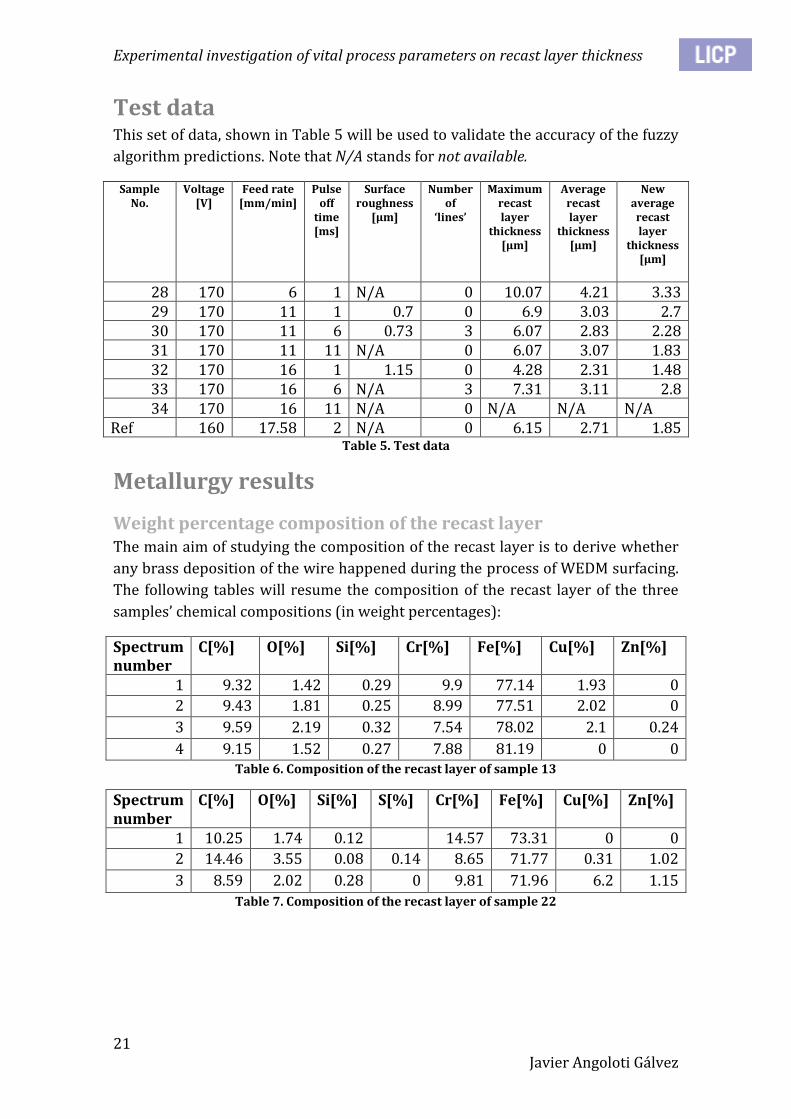
Test data This set of data, shown in Table 5 will be used to validate the accuracy of the fuzzy

algorithm predictions. Note that N/A stands for not available.

Sample No.

Voltage [V]

Feed rate [mm/min]

Pulse off

time [ms]

Surface roughness

[µm]

Number of

‘lines’

Maximum recast layer

thickness [µm]

Average recast layer

thickness [µm]

New average recast layer

thickness [µm]

28 170 6 1 N/A 0 10.07 4.21 3.33 29 170 11 1 0.7 0 6.9 3.03 2.7 30 170 11 6 0.73 3 6.07 2.83 2.28 31 170 11 11 N/A 0 6.07 3.07 1.83 32 170 16 1 1.15 0 4.28 2.31 1.48 33 170 16 6 N/A 3 7.31 3.11 2.8 34 170 16 11 N/A 0 N/A N/A N/A

Ref 160 17.58 2 N/A 0 6.15 2.71 1.85 Table 5. Test data

Metallurgy results

Weight percentage composition of the recast layer The main aim of studying the composition of the recast layer is to derive whether

any brass deposition of the wire happened during the process of WEDM surfacing.

The following tables will resume the composition of the recast layer of the three

samples’ chemical compositions (in weight percentages):

Spectrum number

C[%] O[%] Si[%] Cr[%] Fe[%] Cu[%] Zn[%]

1 9.32 1.42 0.29 9.9 77.14 1.93 0

2 9.43 1.81 0.25 8.99 77.51 2.02 0

3 9.59 2.19 0.32 7.54 78.02 2.1 0.24

4 9.15 1.52 0.27 7.88 81.19 0 0 Table 6. Composition of the recast layer of sample 13

Spectrum number

C[%] O[%] Si[%] S[%] Cr[%] Fe[%] Cu[%] Zn[%]

1 10.25 1.74 0.12 14.57 73.31 0 0

2 14.46 3.55 0.08 0.14 8.65 71.77 0.31 1.02

3 8.59 2.02 0.28 0 9.81 71.96 6.2 1.15

Table 7. Composition of the recast layer of sample 22



Spectrum number

C[%] O[%] Si[%] Cr[%] Fe[%] Cu[%] Zn[%]

1 11.26 2.3 0.24 9.97 73.62 2.18 0.44

2 11.53 1.93 0.3 7.15 77.51 1.58 0

3 9.3 3.43 0.21 11.68 72.2 2.85 0.33

4 10.19 3.61 0.27 13.33 71.93 0.66 0 Table 8. Composition of the recast layer of sample 25

In sample 22, a spectroscopy of the recast layer during the roughing was studied,

to compare if there would be more brass deposition during the said roughing. In

Table 9 the chemical composition of said roughing surface can be seen.

Spectrum number

C[%] O[%] Si[%] S[%] Cr[%] Fe[%] Cu[%] Zn[%]

1 12.60 3.39 0.15 10.90 60.02 10.84 2.11

2 15.01 5.69 0.29 0.41 7.90 54.32 15.26 1.13 Table 9. Composition of the recast layer of the roughing surface in sample 22

Elemental map of recast layer in sample 13 In Figure 10, the different elements found in the recast layer have been mapped

thanks to the spectroscopy.

Figure 10. Elemental map of the recast layer in sample 13

To understand this map, each element was colored differently. The denser the

cloud of points, the higher is the presence of the labeled element. Please note that

zinc and copper have quite light cloud points, mainly due to noisy measurements.



It is interesting to point out that the brass deposition happens in the central part of

the recast layer, close to its surface (note the denser clouds in the windows Cu and

Zn).

The densely dotted chromium islands –in purple- are also remarkable; in the base

metal these chromium islands substitute the steel and are bounded with some

oxygen –in white. This could be chromium oxide (Cr2O3) formed in the surface,

which is the responsible of the anti-corrosion properties of stainless steels6

6 Qiu, J. (2012). Stainless Steels and Alloys: Why They Resist Corrosion and How They Fail.



Statistical analysis

To provide the necessary fuzzy-rules for the fuzzy-networks algorithm, the

experimental data should be analyzed. For this, the Analysis of Variance (ANOVA)

[6] method will be explained–used for the thickness and roughness. Then, a

statistical analysis of regression between the roughness and recast layer thickness

will be discussed. Lastly, a simpler standard deviation test –used to discuss the

chemical compositions- will be explained.

ANOVA model In the case of comparing three independent input variables (Voltage, Pulse off time

and Feed-rate) with an output variable (recast layer thickness or roughness), a

one-way ANOVA analysis suffices to compare that data from these inputs share a

common mean with the output.

This analysis is based in a linear model as follows [8]:

Where:

yij is the output variable (observation), where i is the observation number

and j the different input variables (level); y is denominated a predictor

variable. All y are independent.

βj is the mean of each level, which is a constant for given levels.

εij is the random error, which is normally distributed, with zero mean and a

constant variance: εij ~N(0,σ2).

With ANOVA, the determination if all βj are the same is done, then this analysis is a

hypothesis-based statistical analysis:

Where H0 and H1 are the hypothesis taken into account for the ANOVA. H0 is the

hypothesis that ANOVA will reject, in order to determine which means of each

group are different, i.e. H0 is the null hypothesis.

For discerning the means of the observations, ANOVA divides the variation of the

data into two different groups [9]-[10]:

The variation of group means from the overall mean ( , where is

the mean of group j and the mean of all groups. In other words, the

variation between groups.



The variation of observations in each group from their estimates ( .

In other words, variation within the same group. Note that yij is the output

variable (observation)

ANOVA divides the total sum of squares (SST) into a sum of squares of these

variations (SSR or sum of squares between groups and sum of squared errors or

SSE):

∑∑

∑

∑∑

Where nj is the size of group j.

ANOVA now compares (variation between groups) with (variation

of observations within each group). If the ratio:

is significantly high, the group means are significantly different from each other,

thus the null hypothesis is not satisfied if:

and: ( )

Where:

Fk-1,N-k is an F distribution with k groups and N observations.

( ) is the probability of obtaining results if the null hypothesis

H0 is true.

α is the significance level, which usually is set to 0.05 or 0.01. The

significance level is the probability of rejecting the null hypothesis H0. In

this analysis, α=0.05 will be taken.

In case the p-value is significantly low, this will imply that the recast layer

thickness of roughness varies from different parameters to other. Otherwise, if the

p-value is high (higher than the significance value), this will imply that the output

variable will have low dependence on the different input parameters.



Regression analysis The regression will be measured by the parameter R2, denominated as coefficient

of determination. The more two variables are directly proportional; the closer will

the value of R2 be to 1.

In this case, the variables will be roughness and recast layer thickness; they will be

modeled as if they were linearly proportional.

Using the definitions in the ANOVA model, and introducing the concept of residual

sum of squares (SSR) [8]:

∑

Where fi is the prediction of the i-th value of the recast layer thickness in our case.

Therefore, the coefficient of determination will be:

Arithmetic mean and standard deviation For the discussion of the composition of the recast layer, an arithmetic mean of the

elemental composition of each sample and a calculation of the standard deviation

will be used to explain results.

The arithmetic mean is a simple concept, which will be used to discuss the utility of

the standard deviation. The arithmetic mean of a set of data will be:

∑

Where A is the arithmetic mean, n is the number of data and ai is an individual

result of the data.

The standard deviation σ is a mean of calculating how far apart the scattered

values of data are from the arithmetic mean. For a discrete set of data –as chemical

composition is- it is calculated as follows:

√

∑

In other words, the closer to 0 the standard deviation value is, the closer will the

data be to the mean (the data will be less disperse) –and the results will be more

valid.



Results and discussion of the statistical analysis

ANOVA of recast layer thickness and roughness With the data provided in Table 4 and Table 5, the following results can be derived.

MATLAB was used to provide the results of the ANOVA.

Average recast layer thickness In this case, the output result (thickness of the recast layer) is compared with the

machining inputs (Feedrate, Pulse off time and Voltage):

Sum squared d.f. Mean squared F p>F

Feedrate [mm/min] 3.7072 2 1.85362 1.41 0.2638

Pulse off time [ms] 2.3991 2 1.19957 0.91 0.4154

Voltage [V] 26.1618 3 8.72059 6.62 0.0019 Table 10. ANOVA of the thickness of recast layer

The p-values imply that, for a significance value α=0.05 –which has already been

fixed, the recast layer thickness will be dependent on the Voltage. Feedrate and

Pulse off time will apparently have not a big influence in the output of thickness.

In Figure 11, Figure 12 and Figure 13 the values of each input parameter have been

compared with the mean recast layer thickness each provides, with the use of

multiple comparisons graphs. This gives a more visual interpretation of the

dependence of the thickness with respect of input parameters than the ANOVA

study of the p-value.

In said figures, the dot is the mean recast layer thickness and the whiskers are the

range of recast layer thicknesses each parameter outputs.

Figure 11. Comparison of the Feed-rate with the average thickness



Figure 12. Comparison of the Pulse off time with the average thickness

Figure 13. Comparison of the Voltage with the average thickness

In Figure 13, a low p-value of Voltage for the recast layer thickness with respect to

the significance level α can be deduced, as the thicker the recast layer, the bigger

the Voltage is. The thicknesses referring to 170V are the ones in the training data,

which had different input parameters. If said voltage were to be omitted, the p-

value would still decrease and the multiple comparison graph would corroborate

furthermore the fact that at higher voltages, thicker layer.

As for the dependence on the Feed-rate and Pulse off time, Figure 11 and Figure 12

show the small variation of the outputted thickness with respect to their values.



Recalculated average recast layer thickness In this case, the output result (new calculated thickness of the recast layer) is

compared with the machining inputs (Feedrate, Pulse off time and Voltage):


Feedrate [mm/min] 2.322 2 1.1610 0.64 0.5347

Pulse off time [ms] 2.3692 2 1.1846 0.66 0.5281

Voltage [V] 34.1748 3 11.3916 6.31 0.0026 Table 11. ANOVA of the new recast layer thickness calculated

The results are quite comparable to those in Table 10 although here the Feedrate

and Pulse off time seem to be less important in the generation of thick recast layers

than in the table quoted, as their p-values are higher.

Here there has been no multiple comparisons graphing, as the results are very

similar to those calculated with the former average recast layer thickness.

Roughness In this second case, the output result (roughness) is compared with the machining

inputs (Feedrate, Pulse off time and Voltage):


Feedrate [mm/min] 0.03335 2 0.01667 1.55 0.2646 Pulse off time [ms] 0.23069 2 0.11534 8.04 0.0009 Voltage [V] 0.59027 3 0.19676 15.26 0

Table 12. ANOVA of the roughness

These p-values are comparably lower than the ones obtained in the recast layer

thickness ANOVA test. Nevertheless, the Feedrate, with a p-value that is

significantly high implies that the mean of said Feedrate does not necessarily vary

with respect to the output (roughness). The Pulse off time and Voltage will

significantly vary the roughness, as the p-value is well under the significance level

α=0.05.

In Figure 14, Figure 15 and Figure 16 the values of each input parameter have been

compared with the mean roughness each provides. This, again, gives a more visual

interpretation of the dependence of the thickness with respect of input parameters

than the ANOVA study of the p-value.

The dot is the mean roughness and the whiskers are the range of roughness each

parameter outputs.



Figure 14. Comparison of the Feed-rate with the surface roughness

Figure 15. Comparison of the Pulse off time with the surface roughness

Figure 16. Comparison of the Voltage with the surface roughness



Figure 15 and Figure 16 show the low p-values calculated with ANOVA are

coherent with how the roughness varies with each the Pulse off time and the

Voltage.

As for the Feed-rate, the higher p-value indicates a softer dependence on the

output. Nevertheless, Figure 14 shows a small dependence on the Feed-rate over

the roughness of the samples studied.

Contrasting results derived from ANOVA For the recast layer thickness, both measurements will give a very similar result:

the Voltage is the driving parameter of its formation. Nevertheless, for the

corrected recast layer thickness, the Feedrate and Pulse off time have p-values that

are farther apart from the significance level α, implying a lower dependence of the

formation of the layer with respect to said inputs.

The results of having a recast layer thickness which correlates strongly with the

Voltage are not consistent with those found by the EPFL thesis Experimental

Investigation of Surface Integrity and Defects for a Quality Assurance System of

WEDMed Aerospace Parts [5]; although some papers do find a strong correlation

(p-value<α) between voltage and recast layer thickness [11].

As for the roughness, the Pulse off time is very significant in other papers [5] and

[12] –as found out in this study. Voltage does not appear to have an important role

in the outcome of the mean roughness of the finished piece in the literature,

contrary to what was found in the ANOVA study.

Regression analysis With the data provided in Table 4 and Table 5, two analysis of regression can be

done: between roughness and recast layer thickness and between roughness and

recalculated recast layer thickness.

The software used for this regression analysis has been EXCEL.

Roughness and recast layer thickness In Figure 17, this said regression analysis can be observed. A value of R2=0.2311

implies that roughness and recast layer thickness have not a significant influence

over each other in the experiments done.



Figure 17. Regression analysis between roughness and recast layer thickness

Roughness and new recast layer thickness The regression analysis of the recalculated recast layer thickness can be

appreciated in Figure 18. As in Figure 17, the value of R2 is close to 0.2, hence the

same results can be derived.

Figure 18. Regression analysis between roughness and new recast layer thickness

R² = 0.2311

0

1

2

3

4

5

6

7

8

0 0.2 0.4 0.6 0.8 1 1.2 1.4

Re

cast

la

ye

r th

ick

ne

ss [

μm

]

Roughness [μm]

Correlation between roughness and recast layer thickness

R² = 0.2207

0

1

2

3

4

5

6

7

8

0 0.2 0.4 0.6 0.8 1 1.2 1.4

Re

cast

la

ye

r th

ick

ne

ss [

μm

]

Roughness [μm]

Correlation between roughness and recalculated recast layer thickness



Chemical composition In the following tables, the mean A and standard deviation σ of the data found in

the metallurgical analysis (refer to Table 6, Table 7, Table 8 and Table 9) can be

found. Refer to Table 3 for the composition of the steel used in the samples. For the

calculation of both statistical parameters, EXCEL has been used.

As stated in the past chapter, the closer the standard deviation σ is to 0, the less the

weight percentage of each element changes throughout the recast layer.

Note that in the case of dealing with percentages, the standard deviation calculated

will be in percentage points, not in percentages (the standard deviation of a set of

data has the same units as the set of data, except if the set of data comes in

percentages) [8]. This means, for instance, that if the iron composition from one

sample to another varies from 75% to 80%, the percentage points will increase by

5 percentage points; but in percentages, the augment is:

Composition of the recast layer in sample 13

C O Si Cr Fe Cu Zn

A[%] 9.3725 1.735 0.2825 8.5775 78.465 1.5125 0.06 σ 0.18518 0.34549 0.02986 1.07735 1.8521 1.01072 0.12

Table 13. Mean and standard deviation of the composition in sample 13

The most significant elements present in sample 13 will be carbon, chromium and

carbon. Nevertheless, the values with lowest standard deviation with respect to

their average compositions will be carbon, silicon and iron; being all three and

chromium alloy elements in the base steel.

It can be derived that the composition of the recast layer of sample 13 will have

similar values to those of carbon, silicon and iron averaged. Chromium and oxygen

will also be significantly present along the recast layer. Copper and zinc, not

present as alloys in the stainless steel samples, will appear locally in the recast

layer as a result of the brass wire’s melting.

Composition of the recast layer in sample 22 C O Si S Cr Fe Cu Zn

A[%] 11.1 2.43667 0.16 0.07 11.01 72.3467 2.17 0.72333

σ 3.02590 0.97428 0.10583 0.09899 3.13713 0.83966 3.49352 0.62978 Table 14. Mean and standard deviation of the composition in sample 22

As in sample 13, the most significant elements found will be carbon, chromium and

iron. In this sample, some traces of sulfur were observed (sulfur comes as

impurities in many stainless steels) with not an important outcome. As for the

most significant values, by comparing average percentages and standard



deviations, carbon, oxygen, chromium and iron are the most significant

compositions found during the spectroscopy of sample 22.

Brass (composed of copper and zinc) deposition is significant, but the standard

deviation shows that said deposition will be very scattered throughout the recast

layer.

Composition of the recast layer in sample 25

C O Si Cr Fe Cu Zn

A[%] 10.57 2.8175 0.255 10.5325 73.815 1.8175 0.1925

σ 1.0255 0.82838 0.03872 2.63947 2.57245 0.92981 0.22677 Table 15. Mean and standard deviation of the composition in sample 25

As in the past cases, carbon, chromium and iron are the most present elements in

the recast layer of sample 25. Carbon, silicon and iron will be the elements that

vary the least throughout the recast layer; comparing their respective standard

deviations with their means.

As in the past samples, brass deposition will be scattered through the recast layer,

not being a constant value.

Composition of the roughing recast layer in sample 22

C O Si S Cr Fe Cu Zn

A[%] 13.805 4.54 0.22 0.41 9.4 57.17 13.05 1.62 σ 1.70412 1.6263 0.09899 0.28991 2.12132 4.03050 3.12541 0.69296

Table 16. Mean and standard deviation of the composition in sample 22, rough

This last spectroscopy was made to prove that in the roughing process the brass

deposition can be much higher than in the surfacing process. It is found that,

locally, the brass deposition is important –especially during the roughing. It also

proves that in the micrographs –as seen in Figure 5- the golden colored part is

brass that has been deposited.

Nevertheless, the most significant elements found have been carbon, silicon,

chromium and iron. Brass is also much more present in the roughing than in the

other samples.

Comparison of compositions of the samples In Table 17 the findings of average compositions of the three samples are included.

Sample C O Si S Cr Fe Cu Zn

13 9.3725 1.735 0.2825 - 8.5775 78.465 1.5125 0.06 22 11.1 2.43667 0.16 0.07 11.01 72.3467 2.17 0.72333 25 10.57 2.8175 0.255 - 10.5325 73.815 1.8175 0.1925 22(rough) 13.805 4.54 0.22 0.41 9.4 57.17 13.05 1.62

Table 17. Comparison of the composition of the recast layer of samples studied



The percentage of carbon in the recast layer is higher in comparison with the

percentage of the base stainless steel –which is of around 2% (Table 3) due to the

characteristics of the recast layer, formed due to a fast diffusion of carbon to the

surface as a result of the high heat to which the workpiece is exposed during the

WEDM process. It is due to this carbon that the recast layer is brittle and undesired

for its mechanical properties.

The deposition of brass is significant during the roughing part of the WEDM

process, as the study of the composition shows. Nevertheless, it is also in the

micrographies that this brass deposition can be observed, as seen in Figure 5.

More brass deposition has been observed qualitatively in the zones where there

has been a short-circuit in the wire –also called “lines”- as it can be appreciated in

Figure 19. Note that in the surfacing there have been very few lines or none (refer

to Table 4 and Table 5). The “line” is the concave part; the deposition of brass can

be seen to the right of this concave down section, as well as a white layer that is

cracked. The direction of the wire pass is to the right.

Figure 19. Micrograph of the roughing recast layer with a “line” in sample 26



Main conclusions

Average recast layer thickness Thanks to the ANOVA model, Voltage has been found as the most important driving

parameter influencing the recast layer thickness. Referring to Table 4 and Table 5,

the voltage input can be seen is proportional to the recast layer thickness; at

higher voltages, bigger the thickness.

The recalculation of the recast layer thickness will not vary significantly the

ANOVA results, hence the first approximation of calculation of the recast layer –

where the average thickness was calculated as an arithmetic average- suffices.

Roughness Again, using the ANOVA model, the most important inputs affecting the roughness

of the finished workpiece will be the Pulse off time and Voltage. Pulse off time will

be proportional to the output of roughness as well as the Voltage.

It has also been found that for the samples studied there is no dependence on the

roughness with respect to the recast layer thickness, thanks to the regression

analysis.

Chemical composition The main goal here was to find if there was any brass deposition of the wire in the

recast layer. Although only 3 samples had their chemical compositions studied –

the spectroscopies, as stated, are very time consuming- it could be derived that

there is brass deposition, even after the finishing pass.

All in all, for a better analysis of the composition of the recast layer and how can

the machining parameters affect it, all samples should have their composition

measured, in at least 5 points. After having discussed the results with the average

composition and standard deviation, an ANOVA study should take part in which

each elemental composition is compared to the vital machining parameters. This

would be, as stated before, a very time consuming process; unless the

spectroscopies could be optimized to detect correctly all the elements present in

the recast layer.



References

[1] Various authors. (2015). A FUZZY-NETS FRAMEWORK FOR PREDICTION AND

ADJUSTMENT IN MANUFCATURING PROCESSES. EPF Lausanne.

[2] Ghodsiyeh, D., Golshan, A., Shirvanehdeh, J. A.. (2013). Review on Current

Research Trends in Wire Electrical Discharge Machining (WEDM). Indian Journal of

Science and Technology.

[3] Mahapatra, S. & Patnaik, A. (2006). Parametric optimization of wire electrical

discharge machining (WEDM) process using taguchi method. Journal of the Brazilian

Society of Mechanical Sciences and Engineering, 422-429.

[4] Izquierdo, B., Plaza, B., Sánchez, J.A. , Pomboc, I., Ortegab, N. (2012). Numerical

prediction of heat affected layer in the EDM of aeronautical alloys. Elsevier

[5] Gostimirovic, M., Kovac, P., Sekulic, M., & Skoric, B. (n.d.). Influence of discharge

energy on machining characteristics in EDM. J Mech Sci Technol Journal of

Mechanical Science and Technology, 173-179.

[6] Morand, M. (2014). Experimental Investigation of Surface Integrity and Defects

for a Quality Assurance System of WEDMed Aerospace Parts, 2-5. EPF Lausanne

[7] Hatami, S., Shahabi-Navid, M., & Nyborg, L. (2015). Surface Preparation of

Powder Metallurgical Tool Steels by Means of Wire Electrical Discharge Machining.

Metallurgical and Materials Transactions A, 3215-3226.

[8] Caro, R., Reneses, J. (2012). Manual de estadística. Madrid: Universidad

Pontificia Comillas.

[9] Neter, J., & Wasserman, W. (1974). Applied linear statistical models; regression,

analysis of variance, and0 experimental designs. Homewood, Ill.: R.D. Irwin.

[10] One-Way ANOVA. (2015). The MathWorks, Inc.

[11] Newton, T. (2008). Investigation of the effect of process parameters on the

formation of recast layer in wire-EDM of Inconel 718. Georgia Institute of

Technology, 39-40.

[12] Kurian, A., Yeldose, B., & Mathew, E. (2014). Effect of Wire EDM Parameters on

Surface Roughness of Stainless Steel 15-5 PH. International Journal of Engineering

and Innovative Technology (IJEIT), 88-89.



Annexes

Annex I. Example of the MATLAB code used for the

ANOVA

%%ANOVA of the recast layer with respect to the recast layer thickness

anovan(Averagerecastlayerthicknessmm,{Feedratemmmin,Pulseofftimems,Vol

tageV});

%%Definition of statistics for the multiple comparison graphs [~,~,stats] = anovan(Averagerecastlayerthicknessmm,Feedratemmmin); [~,~,stats1] = anovan(Averagerecastlayerthicknessmm,Pulseofftimems); [~,~,stats2] = anovan(Averagerecastlayerthicknessmm,VoltageV);

%%Multiple comparison graphs [c,~,~,gnames] = multcompare(stats); [c,~,~,gnames] = multcompare(stats1); [c,~,~,gnames] = multcompare(stats2);

Annex II. Measured recast layer thickness samples In this Annex, an example of one micrograph of each of the samples measured will

be included. A digital copy of all the measurements will be available –contact the

author for it.

All optical micrographs have a magnification of 500x. Note that sample 15 is

missing as it could not be unmolded.

Sample 1



Sample 2

Sample 3



Sample 4

Sample 5



Sample 6

Sample 7



Sample 8

Sample 9



Sample 10

Sample 11



Sample 12

Sample 13



Sample 14

Sample 16



Sample 17

Sample 18



Sample 19

Sample 20



Sample 21

Sample 22



Sample 23

Sample 24



Sample 25

Sample 26



Sample 27

Sample 28



Sample 29

Sample 30



Sample 31

Sample 32



Sample 33

Sample Ref 1



Sample Ref 2

Annex II. Electronic micrographs for the

spectroscopy

Sample 13



Sample 22



Sample 22 Rough



Sample 25

ESCUELA TÉCNICA SUPERIOR DE INGENIERÍA (ICAI ...Analysis of Variance –ANOVA- will be done. In...

Documents

Transcript of ESCUELA TÉCNICA SUPERIOR DE INGENIERÍA (ICAI ...Analysis of Variance –ANOVA- will be done. In...