ESCI 241 – Meteorology

Lesson 8 – Thermodynamic Diagrams

Dr. DeCaria

References: The Use of the Skew T, Log P Diagram in Analysis And Forecasting,

AWS/TR-79/006, U.S. Air Force, Revised 1979

An Introduction to Theoretical Meteorology, Hess

GENERAL

� Thermodynamic diagrams are used to display lines representing the major

processes that air can undergo (adiabatic, isobaric, isothermal, pseudo-

adiabatic).

� The simplest thermodynamic diagram would be to use pressure as the y-axis and

temperature as the x-axis.

� The ideal thermodynamic diagram has three important properties

ο The area enclosed by a cyclic process on the diagram is proportional to the

work done in that process

ο As many of the process lines as possible be straight (or nearly straight)

ο A large angle (90°°°° ideally) between adiabats and isotherms

� There are several different types of thermodynamic diagrams, all meeting the

above criteria to a greater or lesser extent. They are the Stuve diagram, the

emagram, the tephigram, and the skew-T/log p diagram

� The most commonly used diagram in the U.S. is the Skew-T/log p diagram.

ο The Skew-T diagram is the diagram of choice among the National Weather

Service and the military.

ο The Stuve diagram is also sometimes used, though area on a Stuve diagram

is not proportional to work.

SKEW-T/LOG P DIAGRAM

� Uses natural log of pressure as the vertical coordinate

ο Since pressure decreases exponentially with height, this means that the

vertical coordinate roughly represents altitude.

� Isotherms, instead of being vertical, are slanted upward to the right.

2

� Adiabats are lines that are semi-straight, and slope upward to the left.

ο The adiabat-isotherm angle is near 90°°°°.

� Pseudoadiabats (moist adiabats) are curved lines that are nearly vertical at the

bottom of the chart, and bend so that they become nearly parallel to the adiabats

at lower pressures.

� Mixing ratio lines (isohumes) slope upward to the right.

BASIC PARAMETERS FOUND FROM SKEW-T DIAGRAM

� The skew-T diagram can be used to determine many useful pieces of information

about the atmosphere.

� The first step to using the diagram is to plot the temperature and dew point

values from the sounding onto the diagram.

ο Temperature (T) is usually plotted in black or blue, and dew point (Td) in

green or red.

� Stability

ο Stability is readily checked on the diagram by comparing the slope of the

temperature curve to the slope of the moist and dry adiabats.

� Mixing ratio (r)

ο Mixing ratio at a given level in the atmosphere is determined by locating the

value of the mixing ratio line that runs through the dew point value at that

level.

� Saturation mixing ratio (rs)

ο Saturation mixing ratio is determined by locating the value of the mixing

ratio line that runs through the temperature value at that level.

� Relative humidity

ο The relative humidity is determined by dividing the mixing ratio by the

saturation mixing ratio.

LIFTING CONDENSATION LEVEL (LCL)

� The lifting condensation level is defined as the level at which an air parcel at the

surface, if lifted dry adiabatically, would reach saturation.

� The LCL is roughly where you would expect cloud bases to be if the mechanism

for upward motion were due to mechanical lifting (such as through orographic

lifting, frontal wedging, or convergence).

� To find the LCL, begin with the surface temperature, and follo

through the surface temperature upward to where it would cross the isohume

(mixing ratio line) that runs through the surface dew

pressure at which they cross is the

LEVEL OF FREE CONVEC

� The level of free convection is the level that the parcel would have to be lifted to

in order for it to be warmer than its environment and start rising on its own.

� There may not be an LFC.

� The LFC is found by first finding the LCL and then followi

upward until it crosses the environmental temperature

LEVEL OF NEUTRAL BUO

� If there is an LFC then as the parcel rises and follows a pseudoadiabat it will

evidentially cross the environmental temperature sounding

point the parcel will be colder than its environment and quit rising.

� This level is called the level of neutral buoyancy, and gives an indication as to

where the tops of any convective clouds will be located.

3

LCL is roughly where you would expect cloud bases to be if the mechanism

for upward motion were due to mechanical lifting (such as through orographic

lifting, frontal wedging, or convergence).

To find the LCL, begin with the surface temperature, and follow the adiabat

through the surface temperature upward to where it would cross the isohume

that runs through the surface dew-point temperature. The

pressure at which they cross is the lifting condensation level.

LEVEL OF FREE CONVECTION (LFC)

The level of free convection is the level that the parcel would have to be lifted to

in order for it to be warmer than its environment and start rising on its own.

There may not be an LFC.

The LFC is found by first finding the LCL and then following a pseudoadiabat

upward until it crosses the environmental temperature sounding.

LEVEL OF NEUTRAL BUOYANCY (LNB)

If there is an LFC then as the parcel rises and follows a pseudoadiabat it will

evidentially cross the environmental temperature sounding again. Past this

point the parcel will be colder than its environment and quit rising.

This level is called the level of neutral buoyancy, and gives an indication as to

where the tops of any convective clouds will be located.

LCL is roughly where you would expect cloud bases to be if the mechanism

for upward motion were due to mechanical lifting (such as through orographic

w the adiabat

through the surface temperature upward to where it would cross the isohume

point temperature. The

The level of free convection is the level that the parcel would have to be lifted to

in order for it to be warmer than its environment and start rising on its own.

ng a pseudoadiabat

If there is an LFC then as the parcel rises and follows a pseudoadiabat it will

again. Past this

This level is called the level of neutral buoyancy, and gives an indication as to

CAPE AND CIN

� Convective available potential energy or CAPE is the energy available to be

converted into kinetic energy of an updraft.

potential for a vigorous updraft and stronger thunderstorm.

� CAPE is proportional to that area on the skew

environmental sounding and the pseudoadiabat connecting the LFC and the

LNB.

� Convective inhibition, or CIN, is the amount of word that an air parcel must

overcome in order to reach the LFC.

� CIN is proportional to that area on the skew

environmental sounding and the path that a parcel from the surface would take

to reach the LFC.

4

Convective available potential energy or CAPE is the energy available to be

converted into kinetic energy of an updraft. The more CAPE, the stronger the

potential for a vigorous updraft and stronger thunderstorm.

CAPE is proportional to that area on the skew-T diagram between the

environmental sounding and the pseudoadiabat connecting the LFC and the

on, or CIN, is the amount of word that an air parcel must

overcome in order to reach the LFC.

CIN is proportional to that area on the skew-T diagram between the

environmental sounding and the path that a parcel from the surface would take

Convective available potential energy or CAPE is the energy available to be

The more CAPE, the stronger the

diagram between the

environmental sounding and the pseudoadiabat connecting the LFC and the

on, or CIN, is the amount of word that an air parcel must

T diagram between the

environmental sounding and the path that a parcel from the surface would take

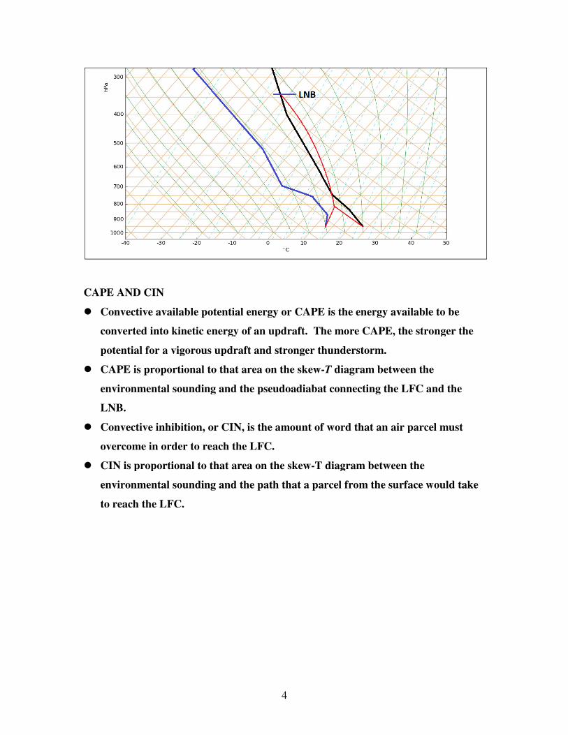
CONVECTIVE CONDENSATION

� The convective condensation level

the bases of convective clouds.

� There are two methods for finding the CCL

ο Method 1 – The mixing method

���� Find the average mixing ratio in the lowest 50 mb or so (by ins

dew-point line), and follow this mixing ratio line up to where it intersects

the temperature sounding.

ο Method 2 – The parcel method

���� Follow the mixing ratio line that passes through the surface dewpoint up

to where it intersects the temperature

���� This is sometimes called the

� These methods will give you roughly the same answer, but not exactly the same

answer.

� The mixing method is more appropriate for finding the bases of deep convective

clouds, such as thunderst

5

ONDENSATION LEVEL (CCL)

convective condensation level is the level at which you would expect to find

the bases of convective clouds.

There are two methods for finding the CCL

The mixing method

Find the average mixing ratio in the lowest 50 mb or so (by ins

point line), and follow this mixing ratio line up to where it intersects

the temperature sounding.

The parcel method

Follow the mixing ratio line that passes through the surface dewpoint up

to where it intersects the temperature sounding.

This is sometimes called the mixing condensation level.

These methods will give you roughly the same answer, but not exactly the same

The mixing method is more appropriate for finding the bases of deep convective

clouds, such as thunderstorms

is the level at which you would expect to find

Find the average mixing ratio in the lowest 50 mb or so (by inspecting the

point line), and follow this mixing ratio line up to where it intersects

Follow the mixing ratio line that passes through the surface dewpoint up

These methods will give you roughly the same answer, but not exactly the same

The mixing method is more appropriate for finding the bases of deep convective

� The parcel method is appropriate for finding the bases of shallow convective

clouds.

� The convective temperature is found by following the adiabat from the CCL to

the surface. This temperature is the temperature at which the surface would

have to reach in order for convective clouds to form.

� Potential temperature (θθθθ

ο The potential temperature

have if it is moved dry

ο It is found by following a dry adiabat through the temperature at a given

level to a pressure of 1000 mb.

6

The parcel method is appropriate for finding the bases of shallow convective

The convective temperature is found by following the adiabat from the CCL to

the surface. This temperature is the temperature at which the surface would

h in order for convective clouds to form.

θθθθ )

The potential temperature is defined as the temperature the parcel would

have if it is moved dry-adiabatically to 1000 mb.

is found by following a dry adiabat through the temperature at a given

level to a pressure of 1000 mb.

The parcel method is appropriate for finding the bases of shallow convective

The convective temperature is found by following the adiabat from the CCL to

the surface. This temperature is the temperature at which the surface would

is defined as the temperature the parcel would

is found by following a dry adiabat through the temperature at a given

7

� Equivalent potential temperature (θθθθe)

ο The equivalent potential temperature is defined as the potential temperature

of the parcel if all of the water vapor in the parcel were condensed and the

latent heat of condensation were used to warm the parcel.

ο The equivalent potential temperature is found by first lifting the parcel to

saturation, then continuing upward along a moist adiabat to the top of the

diagram, and finally descending down a dry adiabat to a pressure of

1000 mb.

� Wet-bulb temperature (Tw)

ο The wet-bulb temperature is found by first lifting the parcel to saturation,

and then following a moist adiabat back down to the parcel’s original level.

� Wet-bulb potential temperature (θθθθw)

ο The wet-bulb potential temperature is found the same way as the wet-bulb

temperature, except that instead of stopping at the original level, continue

down the moist adiabat to 1000 mb.

� Cloud layers

ο In regions where the dew-point depression rapidly decreases with height to

less than 6°°°°C, there is a good possibility of clouds at that level.