
ESBWR IN-PROCESS STATUS FORM - NRC
63
ESBWR IN-PROCESS STATUS FORM Document Title Validation Summary Report for SASSI 2010 and Appendix with Validation Problems for RAI 03.07.02-10 / RAI 03.07.02-26 Response Document Type Shimizu Engineering Report Revision ID (if applicable) SER-DMN-020, Rev.1 (in Shimizu’s doc. number) Author / Responsible Engineer R. Ikeda, Shimizu Corporation Lead R. Ikeda, Shimizu Corporation Date (Last Update/Revision) 6/26/15 Document/Work Status e.g. Pending, Active, On-hold, Complete-In Verification, Verified-Waiting eCM Issued for Use Verification has been performed. (ES1506-V13). Specific Cautions To Users e.g. Enumerate/list specific incomplete content. Enumerate/list specific complete but unverified content. Enumerate/list key areas of technical uncertainty and parameters impacted. Cross-reference Information e.g. eDRF or other useful data pointers
Transcript of ESBWR IN-PROCESS STATUS FORM - NRC

ESBWR IN-PROCESS STATUS FORM Document Title Validation Summary Report for SASSI 2010 and Appendix with
Validation Problems for RAI 03.07.02-10 / RAI 03.07.02-26 Response
Document Type Shimizu Engineering Report
Revision ID (if applicable) SER-DMN-020, Rev.1 (in Shimizu’s doc. number)
Author / Responsible Engineer
R. Ikeda, Shimizu Corporation
Lead R. Ikeda, Shimizu Corporation
Date (Last Update/Revision) 6/26/15
Document/Work Status e.g. Pending, Active, On-hold, Complete-In Verification, Verified-Waiting eCM
Issued for Use Verification has been performed. (ES1506-V13).
Specific Cautions To Users e.g.
Enumerate/list specific incomplete content. Enumerate/list specific complete but unverified content. Enumerate/list key areas of technical uncertainty and parameters impacted.
Cross-reference Information e.g.eDRF or other useful data pointers

Shimizu Engineering Report Project GE-Hitachi Nuclear Energy
Dominion NA 3 ESBWR Project Shimizu Document No. SER-DMN-020
Title Validation Summary Report for SASSI 2010 and Appendix with Validation Problems for RAI 03.07.02-10 / RAI 03.07.02-26 Response
Rev. 1 Issued Date 4/15/15
Revised Date 6/26/15 NOTE:
This document provides Validation Summary Report for SASSI 2010. Appendix with three Validation Problems are also provided for RAI 03.07.02-10 / RAI 03.07.02-26 response. This document is provided in accordance with Reference 1. GEH comments provided in References 2 and 3 are incorporated in this revision.
References: 1. Purchase Order (437080093), Revision 28, dated June 8, 2015 2. E-mail from Ms. Tanya Kirby titled “FW: Action items and notes from April 15
Dominion NRC meeting on July SCP deliverables” dated April 21, 2015 3. E-mail from Mr. Taylor Blake titled “RE: SZGE-ESB-2015-0024 Validation
Summary Report for SASSI2010 and Appendix with Validation Problems for RAI 03.07.02-10 / RAI 03.07.02-26 Response Rev. 0” dated June 24, 2015
1 6/26/15 GEH comments in Appendix A are incorporated Y.O. Y.F. R.I.
0 4/15/15 Initial Issue Y.O. S.O. R.I.
Rev. Date Note Approve Review Prepare Prepared by R. Ikeda 4/15/15
Reviewed by S. Oguri 4/15/15
Approved by Y. Orito 4/15/15
Shimizu Corporation
IMPORTANT NOTICE REGARDING CONTENTS OF THIS REPORT Please Read Carefully
The design, engineering, and other information contained in this document are furnished in accordance with the Development Agreement between Virginia Electric and Power Company and the Consortium of GE-Hitachi Nuclear Energy Americas LLC and Fluor Enterprises, Inc. dated April 5, 2013 as amended. Nothing contained in this document shall be construed as changing the Contract. The use of this information by anyone other than Virginia Electric and Power Company, or for any purpose other than that for which it is furnished by GEH is not authorized; and with respect to any unauthorized use, GEH makes no representation or warranty, express or implied, and assumes no liability as to the completeness, accuracy, or usefulness of the information contained in this document, or that its use may not infringe privately owned rights.
Copyright 2015 GE-Hitachi Nuclear Energy Americas LLC, All Rights Reserved

SER-DMN-020 SH NO. 2
REV. 1 of 9
TABLE OF CONTENTS
1. Purpose ........................................................................................................................................ 3 2. Description .................................................................................................................................. 3
2.1 Computational Modules ........................................................................................................ 3 2.2 Program Limitations ............................................................................................................. 4
3. Software and Hardware Specifications ....................................................................................... 4 3.1 Hardware Specifications ....................................................................................................... 4 3.2 Software Specifications ........................................................................................................ 5
4. Validation and Verification (V&V) ............................................................................................ 6 4.1 Methodology ......................................................................................................................... 6 4.2 Acceptance Criteria ............................................................................................................... 6 4.3 Tested Application Range ..................................................................................................... 7
5. Conclusions ................................................................................................................................. 8 Appendix A SASSI 2010 Validation Problems for RAI 03.07.02-10 / RAI 03.07.02-26
Response ................................................................................................................... 9

SER-DMN-020 SH NO. 3
REV. 1 of 9
1. PURPOSE
This report documents the validation and verification (V&V) of the computer program “SASSI 2010” that is used for the seismic response analysis of structures considering soil structure interaction (SSI) effects.
2. DESCRIPTION
SASSI 2010 is a computer program for seismic response analyses of systems with ability to consider the effects of the interaction of the structure with the surrounding soil/rock that is modeled as a horizontally layered media. The program employs the complex response method, the finite element method and substructuring technique to provide solutions for the seismic response of SSI models in frequency domain.
The SASSI 2010 seismic response analyses provide the following numerical results that serve for developing the basis for seismic design of systems and subsystems:
1. Maximum accelerations and acceleration time histories of the seismic response of the system at different nodal locations
2. Acceleration Response Spectra (ARS) for different damping values at different nodal locations
3. Displacement of the system at different nodal locations relative to the selected reference location or the free field motion
4. Structural member force and stresses 2.1 Computational Modules
The following modules of SASSI 2010 are used to perform the core numerical calculations of the seismic response analysis:
1. SITE that forms and solves transmitting boundary eigenvalue and the site response problem for each specified frequency of analyses (the program models the site as horizontally infinite elastic layers).
2. POINT that provides solutions for the site impedance for each frequency of analysis by applying at surface of the site layers point harmonic loads with frequency equal to the frequency of analysis
3. HOUSE that computes the frequency independent global mass and stiffness matrices for the structure and excavated soil. These global matrices are computed by using different types of finite elements

SER-DMN-020 SH NO. 4
REV. 1 of 9
4. INCOH that computes the incoherency characteristics of the input free-field ground motion with respect to the foundation size and the frequency range of analysis. The SRSS method is used to formulate of influence factors for the modal vectors used in the ground motion input
5. ANALYS that performs the core computations that provide the response of the SSI system under specified input ground motion at each selected frequency of analysis in terms of complex acceleration transfer functions.
6. MOTION that interpolates the acceleration transfer function results from the ANALYS solutions for the selected set of frequencies. It provides the following results for the seismic response at specified nodal locations: a. Interpolated acceleration transfer functions b.Acceleration time histories c. Relative displacement time histories d.Acceleration response spectra, and e. Maximum accelerations and relative displacements
7. STRESS that provides time histories and maximum values for the finite element results for stresses, forces and moments
8. COMBIN that combines the results of two or more different runs of ANALYS module for two or more sets of frequencies of analyses. This module enables multiple computers to be used independently for the analyses of large problems.
2.2 Program Limitations
Number of Fourier transform; 65,536 (Restricted by input column) Number of calculating frequencies : 100 Number of Layers; 100 for layered medium and 20 for simulated halfspace Number of Nodes; 99,999 Number of Interaction nodes; 20,000
3. SOFTWARE AND HARDWARE SPECIFICATIONS
3.1 Hardware Specifications
Hardware used for the SASSI 2010 analysis are commercially available computers installed Microsoft Windows OS.

SER-DMN-020 SH NO. 5
REV. 1 of 9
Operations of data input or execution of the program, etc. should be performed by project members with their client computers through the network system of Shimizu Corporation.
The calculated result files output on computers can be transferred to project member’s client computers through the network, and printed out to the printer set up in Nuclear Project Division.
3.2 Software Specifications
3.2.1 Software module
The software is provided by the form of executable modules in Windows operating system.
3.2.2 Input
Soil Model; Number of layers, thickness of each layer and dynamic properties (unit weight, damping, sear and compression wave velocity) of each layer. Condition at the bottom boundary of the site model; fixed or halfspace modeled by additional layers and viscous dampers to account for geometric damping.
Configuration and properties of finite element structural (HOUSE) model such as node numbering, coordinates and lumped mass inertia properties, interaction nodes, material properties of beam, shell, spring and solid elements that compose the structure model
Parameters defining the frequency domain analysis; Fourier transformation number, time step, analysis frequencies etc. Control motion input data; input acceleration time histories, wave characteristics, control point location.
3.2.3 Process
Complex transfer functions of nodal responses and element stresses are calculated in frequency domain for selected number of frequencies of analysis.
Transfer functions are interpolated for the range of frequencies of interest

SER-DMN-020 SH NO. 6
REV. 1 of 9
Time histories for response in terms of nodal accelerations and finite element stresses are calculated using Fast Fourier Transform and Inverse Fast Fourier Transform.
3.2.4 Output
The echo list of input data
Transfer functions of nodal acceleration responses
Acceleration time histories of response at specified nodal locations
Time histories for stresses at specified elements
4. VALIDATION AND VERIFICATION (V&V)
This chapter describes the test report for validation and verification of SASSI 2010 solutions of seismic response of SSI systems for frequencies up to 70 Hz.
4.1 Methodology
The following methods are used to validate and verify the specified capabilities and limitations of SASSI 2010 program.
i. Comparisons with classical solutions, analytical results or experimental test data published in technical literature,
ii. Comparisons with results obtained from other software
iii. Comparisons of the results from the analyses of various problems and model sizes to validate the program and modeling limitations such as maximum number of soil layers, maximum value of Poisson ratio, maximum element aspect ratio.
4.2 Acceptance Criteria
The acceptance criteria used for the validation and verification are as follows:
NUMERICAL ACCURACY criterion based on requirement that the difference in computed values be less than 1%
GOOD AGREEMENT criterion based on numerical matching against benchmark from classical solutions, analytical results or experimental test data
EXPECTED BEHAVIOR criterion based on basic knowledge and sound engineering judgment

SER-DMN-020 SH NO. 7
REV. 1 of 9
4.3 Tested Application Range
The following capabilities, options and limitations of SASSI 2010 are validated and verified.
1. Calculation of frequency dependent translation and rocking impedance functions
2. Kinematic (wave scattering) SSI solution
3. Ability of the following finite elements to model dynamic properties of structural members and excavated soil:
a. 3-D eight-node solid element
b.3-D beam element
c. Three to four-node quadrilateral thin shell element
d.3-D spring element
4. Solution for seismic response of embedded foundations using flexible volume(direct) method
5. Use of symmetric and anti-symmetric boundary conditions to model and analyze a half model of a structure with symmetry about the two horizontal axes
6. Calculation of response due to incoherent input seismic motion
7. Accuracy of the program post-processing for generation of
a. interpolated transfer functions,
b.maximum accelerations,
c. acceleration response spectra
d. relative displacement time histories
8. Accuracy of calculation of relative displacements from spring element force results.
9. Ability of the following finite elements to accurately calculate stresses, internal forces and moments
a. 3-D beam element,
10. Accuracy of the program different restart options
11. Evaluation of maximum aspect ratio for 3-D solid brick elements and 3-D thin shell elements
12. Evaluation of program ability to model sites using up to 100 horizontally infinite soil layers
13. Evaluation of computed solutions for values of the soil Poisson’s ratio up to 0.48.
14. Evaluation of program ability for analysis of model with a large number of interaction nodes (up to about 20,000 interaction nodes)

SER-DMN-020 SH NO. 8
REV. 1 of 9
15. Accuracy of the program results obtained by combining results from different computer runs
Not all capabilities, features and options of the SASSI 2010 program described in the User’s manual are covered by this validation report. The following are some of the features that are not included in the range of this V&V application:
The program is validated and verified only for seismic analyses of 3-D models. The capability of the program for 2-D analysis is not validated.
No validation and verification is performed of the following types of finite elements:
a. 2-D four-node plane strain element
b.3-D inter-pile element
c. Three to four-node quadrilateral thick shell element
5. CONCLUSIONS
The results of the validation tests meet the corresponding acceptance criteria in Section 4.2. This confirms that the SASSI 2010 computer program is adequate for 3–D seismic response analyses of SSI systems for frequencies up to 70 Hz.

SER-DMN-020 SH NO. 9
REV. 1 of 9
APPENDIX A SASSI 2010 VALIDATION PROBLEMS FOR RAI 03.07.02-10 / RAI 03.07.02-26 RESPONSE
This appendix presents SASSI 2010 Validation Problems. The relationship between the No.s of validation problem and the No.s of application range are shown in Table below. For the validation problems performed using multiple computers, multiple sets of results are presented.
Validation Problem No.
Tested Application Range Page
1 2 3a 3b 3c 3d 4 5 6 7a 7b 7c 7d 8 9a 10 11 12 13 14 15
3 A.3-19 A.9-1
10 A.10-1
A.3 1
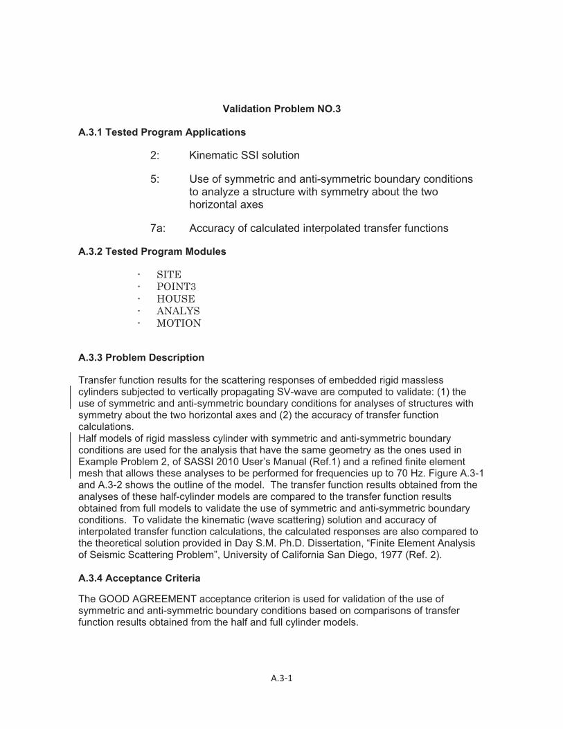
Validation Problem NO.3
A.3.1 Tested Program Applications
2: Kinematic SSI solution
5: Use of symmetric and anti-symmetric boundary conditions to analyze a structure with symmetry about the two horizontal axes
7a: Accuracy of calculated interpolated transfer functions
A.3.2 Tested Program Modules
SITE POINT3 HOUSE ANALYS MOTION
A.3.3 Problem Description
Transfer function results for the scattering responses of embedded rigid massless cylinders subjected to vertically propagating SV-wave are computed to validate: (1) the use of symmetric and anti-symmetric boundary conditions for analyses of structures with symmetry about the two horizontal axes and (2) the accuracy of transfer function calculations. Half models of rigid massless cylinder with symmetric and anti-symmetric boundary conditions are used for the analysis that have the same geometry as the ones used in Example Problem 2, of SASSI 2010 User’s Manual (Ref.1) and a refined finite element mesh that allows these analyses to be performed for frequencies up to 70 Hz. Figure A.3-1 and A.3-2 shows the outline of the model. The transfer function results obtained from the analyses of these half-cylinder models are compared to the transfer function results obtained from full models to validate the use of symmetric and anti-symmetric boundary conditions. To validate the kinematic (wave scattering) solution and accuracy of interpolated transfer function calculations, the calculated responses are also compared to the theoretical solution provided in Day S.M. Ph.D. Dissertation, “Finite Element Analysis of Seismic Scattering Problem”, University of California San Diego, 1977 (Ref. 2).
A.3.4 Acceptance Criteria
The GOOD AGREEMENT acceptance criterion is used for validation of the use of symmetric and anti-symmetric boundary conditions based on comparisons of transfer function results obtained from the half and full cylinder models.

A.3 2
The GOOD AGREEMENT acceptance criterion is used for validation of the kinematic (wave scattering) solution and accuracy of interpolated transfer function calculations based on comparisons of calculated responses with theoretical solution.
A.3.5 Modeling
The SASSI soil layer models consist of top layers resting on the surface of a halfspace. The halfspace is modeled by 40 uniform layers with thickness of 8.125 ft and additional 10 layers with varying thickness as a function of frequency and a viscous boundary at the base. The site model is shown in Fig. A.3-1. The input soil properties are summarized in Table A.3-1.
The foundations are rigid massless cylinders with a radius (R) of 65 ft and are fully embedded to a depth of 32.5 ft. The geometry of the foundation cross-sections are shown in Fig. A.3-2. Stiff material properties are assigned to the cylinder model to ensure the rigidness of the foundation.
A.3.5.1 Excavated Soil Models
The nodes and the elements of the excavated soil half model at elevations -32.5, -24.375, -16.25, -8.125 and 0. ft, are shown in Figs. A.3-3, A.3-4, A.3-5, A.3-6, and A.3-7, respectively. The maximum size of the finite elements is 10.364 ft which is less than 20% of the wavelength of seismic waves with frequency of 70 Hz.
A.3.5.2 Structural Models
The cylinder foundations are discretized using brick elements. The nodes and elements of the foundation model are shown in Figs. A.3-8 through A.3-12.
A.3.5.3 SSI Frequencies and Wave Fields
The SASSI analysis for this problem is performed for frequencies up to 70 Hz as shown in Table A.3-2. These frequencies of analysis are determined from the product of frequency step (DF) and the frequency numbers (NF):
F = DF * NF
DF is set to 0.02 Hz. The control motion is specified to be vertically propagating SV-wave with a control point defined at the ground surface.
A.3.5.4 Analysis Cases
The SASSI runs for this validation test problem consists of 3 of seismic analysis cases. The analysis models for the considered 3 cases are summarized in Table A.3-3.

A.3 3
The SASSI analyses have been performed using seismic excitation in the form of vertically propagating SV-waves. The SASSI sequence of runs and input/output files for this problem are shown in Table A.3-4.
A.3.6 Analysis Results
The SASSI results for the responses of foundation central node from the analyses of the three models are shown in Figs. A.3-13 and A.3-14. The comparison of these results shows that the good agreement acceptance criteria is met over the frequency range of analysis.
A.3.7 Conclusion
The good agreement of the responses obtained from the analyses of the full model and the half models with symmetric and anti-symmetric boundary conditions validates the accuracy of the results obtained from the SASSI2010 analyses of half models with symmetric and anti-symmetric boundary conditions. This validated the SASSI2010 ability for analysis of half models of structures with symmetry about the two horizontal axes.
A.3.8 References
1. Computer Program SASSI2010 – User’s Manual, May 2012.
2. Day, S. M., "Finite Element Analysis of Seismic Scattering Problem," Ph.D. Dissertation, University of California, San Diego, 1977.

A.3 4
Table A.3-1 Soil Properties Layer No.
Top EL [ft]
Layerthickness
[ft]
Unitweight[pcf]
Vs[ft/sec]
Vp[ft/sec]
Damping [%] Remark
1 0.0 8.125 126.68 3700.0 6409.0 1.02 -8.125 8.125 126.68 3700.0 6409.0 1.03 -16.25 8.125 126.68 3700.0 6409.0 1.04-39 -24.375 8.125 126.68 3700.0 6409.0 1.040 -316.875 8.125 126.68 3700.0 6409.0 1.0
-325.00 - 126.68 3700.0 6409.0 1.0 Halfspace

A.3 5
Table A.3-2 Frequencies of Analysis NF f (Hz) a0 NF f (Hz) a0 1 0.02 0.002 1800 36.00 3.97450 1.00 0.110 1850 37.00 4.084100 2.00 0.221 1900 38.00 4.194150 3.00 0.331 1950 39.00 4.305200 4.00 0.442 2000 40.00 4.415250 5.00 0.552 2050 41.00 4.526300 6.00 0.662 2100 42.00 4.636350 7.00 0.773 2150 43.00 4.746400 8.00 0.883 2200 44.00 4.857450 9.00 0.993 2250 45.00 4.967500 10.00 1.104 2300 46.00 5.077550 11.00 1.214 2350 47.00 5.188600 12.00 1.325 2400 48.00 5.298650 13.00 1.435 2450 49.00 5.409700 14.00 1.545 2500 50.00 5.519750 15.00 1.656 2550 51.00 5.629800 16.00 1.766 2600 52.00 5.740850 17.00 1.876 2650 53.00 5.850900 18.00 1.987 2700 54.00 5.961950 19.00 2.097 2750 55.00 6.0711000 20.00 2.208 2800 56.00 6.1811050 21.00 2.318 2850 57.00 6.2921100 22.00 2.428 2900 58.00 6.4021150 23.00 2.539 2950 59.00 6.5121200 24.00 2.649 3000 60.00 6.6231250 25.00 2.760 3050 61.00 6.7331300 26.00 2.870 3100 62.00 6.8441350 27.00 2.980 3150 63.00 6.9541400 28.00 3.091 3200 64.00 7.0641450 29.00 3.201 3250 65.00 7.1751500 30.00 3.311 3300 66.00 7.2851550 31.00 3.422 3350 67.00 7.3951600 32.00 3.532 3400 68.00 7.5061650 33.00 3.643 3450 69.00 7.6161700 34.00 3.753 3500 70.00 7.7271750 35.00 3.863

A.3 6
Table A.3-3 Cases of Validation Problem No.3 Case No Model Remark
1 XZ-Symmetry Half Model
2 Y-Anti-Symmetry Half Model
3 Full Model Full Mode
Table A.3-4 Input/Output Files of Validation Problem No.3
SASSI SEQUENCE OF RUNS SASSI MODULE
INPUT OUTPUT TAPEIN TAPEOUT
SITE vv08cN*ex2_site.dat vv08cN*ex2_site.txt SASSI.T1 SASSI.T2
POINT vv08cN*ex2_point.dat vv08cN*ex2_point.txt SASSI.T2 SASSI.T3HOUSE Cylinder_Full.hou
Cylinder_Half-sym-xz.houCylinder_Half-anti-y.hou
vv08cN*ex2_house.txtSASSI.T4
ANALYS vv08cN*ex2_analys.dat vv08cN*ex2_analys.txt SASSI.T1 SASSI.T3 SASSI.T4
SASSI.T8
MOTION vv08cN*ex2_motion.dat vv08cN*ex2_motion.txt SASSI.T8 SASSI.T13 N*: Case number 1,2,3

A.3 7
Figure A.3–1. SASSI Soil Layer Model
Figure A.3–2. Geometry of Cylinder Foundation Cross Section
325
335
345
355
365
(40)
EL 0.000
EL 8.125
EL 16.250
EL 24.375
EL 325.000

A.3 8
Figure A.3–3. Excavated Soil Model at Elevation –32.5 ft
Figure A.3–4. Excavated Soil Model at Elevation –24.375 ft

A.3 9
Figure A.3–5. Excavated Soil Model at Elevation –16.25 ft
Figure A.3–6. Excavated Soil Model at Elevation –8.125 ft

A.3 10
Figure A.3–7. Excavated Soil Model at Elevation 0 ft
Figure A.3–8. Cylinder Foundation Model at Elevation –32.5 ft

A.3 11
Figure A.3–9. Cylinder Foundation Model at Elevation –24.375 ft
Figure A.3–10. Cylinder Foundation Model at Elevation –16.25 ft

A.3 12
Figure A.3–11. Cylinder Foundation Model at Elevation –8.125 ft
Figure A.3–12. Cylinder Foundation Model at Elevation 0 ft

A.3 13
Figure A.3–13. Response of Foundation due to Vertically Propagating SV-wave (Translational)
Figure A.3–14. Response of Foundation due to Vertically Propagating SV-wave (Rocking)
0.0
0.2
0.4
0.6
0.8
1.0
1.2
0 1 2 3 4 5 6 7 8
Normalize
dTran
slationa
lRespo
nse
Dimensionless frequency a0=2 fR/Vs
Day's Solution
XZ Symmetry X Dir (SASSI2010)
Y Anti Symmetry Y Dir (SASSI2010)
Full Model X Dir (SASSI2010)
0.0
0.2
0.4
0.6
0.8
1.0
1.2
0 1 2 3 4 5 6 7 8
Normalize
dRo
ckingRe
spon
se
Dimensionless frequency a0=2 fR/Vs
Day's Solution
XZ Symmetry Z Dir (SASSI2010)
Y Anti Symmetry Z Dir (SASSI2010)
Full Model Z Dir (SASSI2010)

A9 1
Validation Problem NO.9
A.9.1 Tested Program Applications
2: Kinematic SSI solution for frequencies up to 70 Hz
A.9.2 Tested Program Modules
SITE POINT3 HOUSE ANALYS MOTION
A.9.3 Problem Description Seismic response analyses are performed of a rigid massless cylinder embedded in a halfspace and subjected to vertically propagating SV waves. Section A3.3 describes the half model with symmetry conditions used for the SSI analyses that is same as the one used in Validation Problem No. 3 and is more refined than Example Problem 2 of SASSI 2010 User’s Manual (Ref. 1). Transfer function results are calculated for frequencies up to 70 Hz for the response at the bottom of the cylinder and compared with to the theoretical solution provided in Day S.M. Ph.D. Dissertation, “Finite Element Analysis of Seismic Scattering Problem“, University of California San Diego, 1977 (Ref. 2). A.9.4 Acceptance Criteria
The GOOD AGREEMENT acceptance criterion is used for validation of the SASSI2010 kinematic (wave scattering) solution for frequencies up to 70 Hz based on comparisons of calculated responses with theoretical solutions.
A.9.5 Modeling
The SASSI soil layer models consist of top layers and halfspace. Depending on the embedment depth considered, the top layers used are 40 layers. Each of the top layers has a thickness of 8.125 ft. The halfspace is modeled by an additional 10 layers with varying thicknesses as a function of frequency and a viscous boundary at the base. The 40-top-layer site model is shown in Figs A.9-1. The shear-wave velocity (Vs) and P-wave velocity (Vp) of the soil layers are summarized in Table A.9-1. The used soil properties are:
Weight Density = 128.68 pcf

A9 2
Poisson's Ratio = 1/4 Material Damping = .01
Note that the halfspace in all cases has the same shear-wave velocity (Vs=3700 ft/sec) and P-wave velocity (Vp= 6409 ft/sec). The foundations are rigid massless cylinders with a radius (R) of 65 ft and are fully embedded to a depth of 32.5 ft. Geometries of the foundation cross-sections are shown in Fig. A.9-2. High stiffness properties are used to ensure the rigid foundation behavior.
A.9.5.1 Excavated Soil Models The nodes and the elements of the excavated soil half model at elevations -32.5, -24.375, -16.25, -8.125 and 0. ft, are shown in Figs. A.9-3, A.9-4, A.9-5, A.9-6, and A.9-7, respectively. The maximum size of the finite elements is 10.364 ft which is less than 20% of the wavelength of seismic waves with frequencies of 70 Hz. A.9.5.2 Structural Models
The cylinder foundations are discretized using brick elements. The nodes and elements of the foundation model are shown in Figs. A.9-8 through A.9-12. A.9.5.3 SSI Frequencies and Wave Fields The SASSI analysis for this problem is performed for frequencies shown in Table A.9-2. These frequencies are determined from the product of frequency step (DF) and the frequency numbers (NF):
f = DF * NF (A.9-1)
In the analysis, DF is specified as 0.02 Hz. The dimensionless frequency ratio a0 shown in Table A.9-2 is computed from
a0 = 2 fR / Vs (A.9-2)
Where R is the radius of the cylinder and Vs is the shear wave velocity of the soil material. Note that the a0 definition is only applicable to this problem. Also note that the model mesh constructed for this problem is valid up to the frequency limit of 70.0 Hz corresponding to a0 = 7.7. The control motion is specified as vertically propagating SV-wave with a control point defined at the ground surface.

A9 3
A.9.5.4 Analysis Cases
The SASSI analyses have been performed using seismic excitation in the form of vertically propagating SV-waves. The SASSI sequence of runs and input/output files for this problem are shown in Table A.9-3.
The flexible volume (direct) method is used where all nodes in the excavated soil volume are defined as interaction nodes. The results of analyses are compared with the reference solution in Reference 2. A.9.6 Analysis Results The amplitude of the translational response motion at Node 1 (|U1x|) and the amplitude of the rocking motion (|U66z|, assuming that |U1z| is negligible) of the foundation subjected to vertically propagating SV-waves is normalized to the amplitude of free-field motion (Uo=1) and plotted in Figs. A.9-13 and A.9-14, respectively. The results are compared with results reported by Day(1977) (Ref. 2). The comparison with theoretical solution demonstrates that SASSI2010 results satisfy the good agreement acceptance criteria. A.9.7 Conclusion
The good agreement obtained between SASSI2010 results and the reference solution (Ref. 2) validates the SASSI2010 calculations of frequency dependent translation and rocking impedance functions for embedded structures and the acceptability of computed solutions up to frequency of 70 Hz. A.9.8 References
1. Computer Program SASSI2010 – User’s Manual, May 2012. 2. Day, S. M., "Finite Element Analysis of Seismic Scattering Problem," Ph.D. Dissertation, University of California, San Diego, 1977.

A9 4
Table A.9-1. Cases of Example Problem
Case No
Embedment Depth (ft) Vs and Vp (ft/sec) Seismic Loading
1 32.5 (4 layers) Vs=3700.0 & Vp=6409.0 Vertically Propagating SV-wave
Table A.9-2. Frequencies of Analysis
NF f (Hz) a0 NF f (Hz) a0 1 0.02 0.002 1800 36.00 3.974 50 1.00 0.110 1850 37.00 4.084 100 2.00 0.221 1900 38.00 4.194 150 3.00 0.331 1950 39.00 4.305 200 4.00 0.442 2000 40.00 4.415 250 5.00 0.552 2050 41.00 4.526 300 6.00 0.662 2100 42.00 4.636 350 7.00 0.773 2150 43.00 4.746 400 8.00 0.883 2200 44.00 4.857 450 9.00 0.993 2250 45.00 4.967 500 10.00 1.104 2300 46.00 5.077 550 11.00 1.214 2350 47.00 5.188 600 12.00 1.325 2400 48.00 5.298 650 13.00 1.435 2450 49.00 5.409 700 14.00 1.545 2500 50.00 5.519 750 15.00 1.656 2550 51.00 5.629 800 16.00 1.766 2600 52.00 5.740 850 17.00 1.876 2650 53.00 5.850 900 18.00 1.987 2700 54.00 5.961 950 19.00 2.097 2750 55.00 6.071 1000 20.00 2.208 2800 56.00 6.181 1050 21.00 2.318 2850 57.00 6.292 1100 22.00 2.428 2900 58.00 6.402 1150 23.00 2.539 2950 59.00 6.512 1200 24.00 2.649 3000 60.00 6.623 1250 25.00 2.760 3050 61.00 6.733 1300 26.00 2.870 3100 62.00 6.844 1350 27.00 2.980 3150 63.00 6.954 1400 28.00 3.091 3200 64.00 7.064 1450 29.00 3.201 3250 65.00 7.175 1500 30.00 3.311 3300 66.00 7.285 1550 31.00 3.422 3350 67.00 7.395 1600 32.00 3.532 3400 68.00 7.506 1650 33.00 3.643 3450 69.00 7.616 1700 34.00 3.753 3500 70.00 7.727 1750 35.00 3.863

A9 5
Table A.9-3. Input/Output Files of Validation Problem 9 – Case 1 VERTICALLY PROPAGATING SV ANALYSIS
SASSI MODULE
INPUT OUTPUT TAPEIN TAPEOUT
SITE vv16c3r8vsd.dat vv16c3r8vso.out - SASSI.T1 SASSI.T2
POINT3 E2C1PD.dat vv16c3r8po.out - SASSI.T3 HOUSE Cylinder_Half-
sym-xz.hou vv16c3r8vho.out - SASSI.T4
SASSI.T7 ANALYS E2C1AD.dat vv16c3r8ao.out SASSI.T1
SASSI.T3 SASSI.T4
SASSI.T5 SASSI.T8
MOTION E2C1VOD.dat vv16c3r8voo.out SASSI.T8 SASSI.T13
Figure A.9–1. SASSI Soil Layer Model
(40)
EL 0.000
EL 8.125
EL 16.250
EL 24.375
EL 325.000

A9 6
Figure A.9–2. Geometry of Cylinder Foundation Cross Section

A9 7
Figure A.9–3. Excavated Soil Model at Elevation –32.5 ft
Figure A.9–4. Excavated Soil Model at Elevation –24.375 ft

A9 8
Figure A.9–5. Excavated Soil Model at Elevation –16.25 ft
Figure A.9–6. Excavated Soil Model at Elevation –8.125 ft

A9 9
Figure A.9–7. Excavated Soil Model at Elevation 0 ft
Figure A.9–8. Cylinder Foundation Model at Elevation –32.5 ft

A9 10
Figure A.9–9. Cylinder Foundation Model at Elevation –24.375 ft
Figure A.9–10. Cylinder Foundation Model at Elevation –16.25 ft

A9 11
Figure A.9–11. Cylinder Foundation Model at Elevation –8.125 ft
Figure A.9–12. Cylinder Foundation Model at Elevation 0 ft

A9 12
Figure A.9–13. Response of Foundation due to Vertically Propagating SV-Wave
(Translation Response, Case1)
Figure A.9–14. Response of Foundation due to Vertically Propagating SV-Wave (Rocking Response, Case1)
0.0
0.2
0.4
0.6
0.8
1.0
1.2
0 1 2 3 4 5 6 7 8
Nor
mal
ized
Tra
nsla
tiona
l Res
pons
e
Dimensionless Frequency a0=2 fR/Vs
Translational Response due to Horizontally Propagating SV-Waves
Day's Solution
SASSI2010
0.0
0.2
0.4
0.6
0.8
1.0
1.2
0 1 2 3 4 5 6 7 8
Nor
mal
ized
Roc
king
Res
pons
e
Dimensionless Frequency a0=2 fR/Vs
Rocking Response due to VerticalyPropagating SV-Waves
Day's Solution
SASSI2010

A.10 1
Validation Problem NO.10
A.10.1 Tested Program Applications
11: Evaluation of maximum aspect ratio for 3-D solid brick elements and 3-D thin shell elements
A.10.2 Tested Program Modules
SITE POINT3 HOUSE ANALYS MOTION
A.10.3 Problem Description
A seismic response analysis is performed on the ESBWR control building (CB) model (Ref.2, 3) to establish the maximum acceptable aspect ratio for 3-D solid brick elements and 3-D thin shell elements. Figure A.10-1 shows the CB model consisting of a lumped mass stick model representing the dynamic properties of the building above grade, 3-D thin shell elements modeling the below grade exterior walls and the foundation basemat and 3-D solid elements modeling excavated soil volume and the concrete fill placed around and below the foundation. The meshes of the concrete fill and excavated soil volume models are consistent with the mesh of the shell element models of the basemat and below grade exterior walls.
Seven models of ESBWR CB are developed with meshes that have aspect ratio of 1:1.3, 1:1.5, 1:1.7, 1:2, 1:3 and 1:4. The maximum aspect ratios of the model shown in Figure A.10-1 are 1:1.5 for the 3-D solid brick elements and 1:1.7 for the 3-D thin shell elements. Seismic response analyses are performed on the models with different meshes with the input free field in layer control motion applied at bottom of the CB foundation. The results for maximum absolute accelerations and acceleration response spectra obtained from the analyses of the different CB models are compared in order to evaluate the acceptability of the used element aspect ratio.
A.10.4 Acceptance Criteria The evaluation of maximum acceptable aspect ratio for 3-D solid and thin shell elements is based on
NUMERICAL ACCURACY criterion that is used for comparison of maximum acceleration results
obtained from the models with different meshes
GOOD AGREEMENT criterion that is used for comparison of acceleration response spectra results
obtained from the models with different meshes
A.10.5 Analysis Model
Figure A.10-1 shows the analysis model considered in this validation problem. The model consists of single stick model, and the exterior walls below grade and the foundation basemat along with the supporting soil medium and the backfill surrounding the building. The stick model is a three-dimensional lumped mass-beam model that considers shear, bending, torsion and axial deformations. In this model, the basemat and the exterior walls are modeled by plate elements. The excavated soil volume elements are part of the structural

A.10 2
models. The excavated soil volumes have mesh that is consistent with the FE mesh of the basemat and basement exterior walls finite elements. The excavated soil elements are assigned with in-situ strain compatible soil properties as the ones used in the site profile models representative of a typical rock site in Central and Eastern US (Ref. 3).
The maximum aspect ratios of the model shown in Fig. A.10-1are about 1:1.5 for the 3-D solid brick elements and 1:1.7 for the 3-D thin shell elements. The various analytical models with various maximum aspect ratios, 1:1.3, 1:2, 1:3 and 1:4 are produced, and earthquake response analyses are performed.
The acceleration time history of the motion specified at the bottom of the basemat, EL -10.4m is shown in Fig. A.10-2. The input wave has maximum acceleration of 0.73g with duration of 40.96 seconds digitized at time intervals of 0.005 second. The cut-off frequency used for the analysis is 50 Hz.
A.10.5.1 Soil Model
The maximum allowable layer thickness is computed according to the criterion described in item 8 of Section 4.2.2 (Ref. 1):
Maximum allowable thickness = 616[m/sec]/(5 x 50[Hz]) = 2.46m
Based on this value, the soil profile for the SASSI analysis is selected as shown in Table A.10-1 and Table A.10-2. This profile consists of 17 top layers and 10 extra layers with variable thickness plus viscous dashpots. The extra 10 layers and viscous dashpots are added by the program at the user's request to simulate a halfspace condition.
A.10.5.2 Structural Model
The structural finite element model used in the SASSI analysis is shown in Fig. A.10-3. The structures are modeled by stick model (in black), plate (in blue), and rigid beams elements (in red). The stick model consists of lumped masses and beam elements as shown in Fig. A.10-4. A uniform SSE damping of 7% was used for the structural model. The basemat is modeled with plate elements with stick model connected with using the rigid beams to be able to transmit the moment/rotation at the connection.
The wavelength criterion described in item 9 of Section 4.2.2(Ref. 1) is used to select the element sizes of the plate elements in the all directions.
Maximum allowable element size = 616[m/sec]/(5 x 50[Hz]) = 2.46m
A.10.5.3 Excavated Soil Model
Mesh size for Excavated Soil Model is determined by using soil profile shown in Table A.10-1.
A. 10.5.4 Mesh Size
Mesh size for Excavated Soil Model including concrete fill and CB exterior walls are shown in Fig.A.10-5. The maximum aspect ratio of 3-D solid brick elements is 1:1.5. The maximum aspect ratio of 3-D thin shell element below grade is 1:1.7.

A.10 3
A.10.6 Analyses Cases
The SASSI runs for this validation test problem consists of 7 cases. The aspect ratios for the 7 cases are summarized in Table A.10-3. The original mesh size of the model in Ref.3 is shown in Fig. A.10-5 and is referred to as the case 2 model. Other models defined in Table A.10-3 are derived from case 2 model for other aspect ratios.
Aspect ratio of each case is set by the H0, H1, H2, H3, H4, H5 and W1, W2, W3 parameters as shown in Figs. A.10-6 through A.10-12.
A.10.7 Results and Comparison
The SASSI sequence of runs and input/output files for this validation problem are shown in Table A.10-4. This table also includes the names that are assigned to the tapes for conveniences of tapein / tapeout activity.
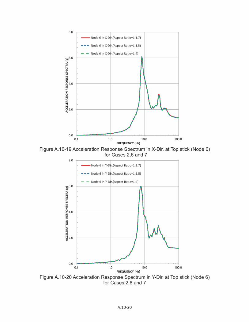
Tables A.10-5 and A.10-6 show the maximum absolute acceleration at the top of the stick outer walls and the nodes associated with the elements having the maximum aspect ratios obtained from the various SASSI models with different element mesh. The maximum acceleration values obtained from the different CB models are almost the same with minor differences less than 2%, thus demonstrating that the NUMERICAL ACCURACY criterion is satisfied.
The 5% acceleration spectrums are computed for the horizontal motions at the top of the stick outer walls, top of Basemat and the nodes associated with the elements having the maximum aspect ratios. The comparisons of the results obtained from the analyses of the seven models are presented in Figs. A.10-13 through A.10-36. The comparisons of the acceleration response spectra results demonstrate that the good agreement criterion is met for all CB models with different mesh.
A.10.8 Conclusion
The comparison in Table A.10-5 of the maximum acceleration results demonstrate that the NUMERICAL ACCURACY criterium is satisfied. The good agreement is demonstrated in Figs. A.10-13 throught A.10-36 between the acceleration response spectra results from the models with five different meshes and. Therefore, the maximum aspect ratio of 1:4 for 3-D solid brick elements and 3-D thin shell is validated.
A.10.9 References 1. Computer Program SASSI2010 – User’s Manual, May 2012.
2. 26A6642AL, ESBWR Design Control Document Tier 2 Chapter 3 Appendices 3A – 3F, Rev. 9, Dec. 2010.
3. SER-DMN-003, CB Licensing Basis Seismic Analysis Report (Basis document for FSAR Markup), Dominion NA3 ESBWR Project, Dec. 2013.

A.10 4
Table A.10-1 Soil Properties Layer No.
Top EL [m]
Layer thickness
[m]
Unitweight
[ton/m3]
Vs[m/sec]
Vp[m/sec]
Damping[%] Remark
1 -3.12 1.525 2.32 616 1882 6.2 2 -4.645 1.525 2.32 616 1882 6.2 3 -6.17 1.230 2.32 753 2301 6.3 4 -7.40 1.500 2.32 753 2301 6.3 5 -8.90 1.500 2.32 753 2301 6.3 6 -10.40 1.860 2.32 753 2301 6.3 7 -12.26 1.525 2.32 810 2474 5.3 8 -13.785 1.525 2.32 810 2474 5.3 9 -15.31 3.050 2.61 1976 4225 1.0
10 -18.36 6.100 2.61 2128 4273 1.0 11 -24.46 3.040 2.61 2421 4613 1.0 12 -27.50 3.050 2.63 2638 4772 1.0 13 -30.55 3.050 2.63 2512 4787 1.0 14 -33.60 3.050 2.63 2639 4937 1.0 15 -36.65 3.050 2.63 2689 4722 1.0 16 -39.70 3.040 2.63 2847 5150 1.0 17 -42.74 3.050 2.63 2804 5245 1.0
-45.79 - 2.63 2804 4794 1.0 halfspace
Table A.10-2 Backfill Properties for CB Layer No.
Top EL [m]
Layer thickness
[m]
Unitweight
[ton/m3]
Vs[m/sec]
Vp[m/sec]
Damping[%] Remark
- - - 2.32 2134 3325 1.0
Table A.10-3 Case of Validation Problem No.10 Case Max. Aspect Ratio H0(mm) H1(mm) W1(mm) W2(mm) W3(mm) H2(mm) H3(mm) H4(mm) H5(mm) RemarkNo Brick
ElementShell
Element
1 1:1.3 1:1.7 1427.0 1636.7 1865.0 1865.0 - 1100.0 1100.0 1000.0 1120.0 2 1:1.5 1:1.7 1230.0 1860.0 1240.0 1240.0 1250.0 1100.0 1100.0 1000.0 1120.0 3 1:2 1:1.7 1230.0 1860.0 930.0 1400.0 1400.0 1100.0 1100.0 1000.0 1120.0 4 1:3 1:1.7 1230.0 1860.0 620.0 1555.0 1555.0 1100.0 1100.0 1000.0 1120.0 5 1:4 1:1.7 1230.0 1860.0 465.0 1632.5 1632.5 1100.0 1100.0 1000.0 1120.0 6 1:1.3 1:1.5 1427.0 1636.7 1865.0 1865.0 - 1300.0 1300.0 1300.0 1120.0 7 1:1.3 1:4 1427.0 1636.7 1865.0 1865.0 - 425.0 1775.0 1000.0 1120.0

A.10 5
Table A.10-4 Input/Output Files of Validation Problem No.10 SASSI SEQUENCE OF RUNS
SASSI MODULE
INPUT OUTPUT TAPEIN TAPEOUT
SITE V17_site.dat V17_site.out - V17_T1 V17_T2
POINT V17_pointN*.dat V17_pointN*.out V17_T2 V17_T3_CN* HOUSE V17_houseN*.dat V17_houseN*.out V17_T4_CN* ANALYS V17_analys.dat V17_analysN*.out V17_T1_CN*
V17_T4_CN* V17_T5_CN*
V17_T6_CN* V17_T8_CN*
MOTION V17_motion.dat V17_motionN*.out V17_T8_CN* V17_T12_CN*
N*: Case number 1,2,3,4,5,6,7
Table A.10-5 Maximum Acceleration at Top of StickCase No Max Aspect Ratio X-dir
[g]Y-dir [g]
Z-dir[g]Brick
ElementShell
Element1 1:1.3 1:1.7 1.328 1.157 1.137 2 1:1.5 1:1.7 1.343 1.156 1.141 3 1:2 1:1.7 1.344 1.155 1.142 4 1:3 1:1.7 1.345 1.155 1.143 5 1:4 1:1.7 1.345 1.155 1.143 6 1:1.3 1:1.5 1.328 1.157 1.137 7 1:1.3 1:4 1.329 1.157 1.137
Max. Difference (%) 1.3 0.2 0.5
Table A.10-6 Maximum Acceleration at NodesCase Max. Aspect Ratio Node 1170 or 1234 Node 1426 Node 16488 or 16513 Node 8380 No Brick
ElementShell
ElementX-dir [g]
Y-dir [g]
Z-dir [g]
X-dir[g]
Y-dir[g]
Z-dir[g]
X-dir[g]
Y-dir[g]
Z-dir [g]
X-dir [g]
Y-dir[g]
Z-dir[g]
1 1:1.3 1:1.7 - - - - - - 0.460 0.471 0.818 0.413 0.401 0.7022 1:1.5 1:1.7 - - - 0.678 0.836 0.722 0.463 0.467 0.817 0.420 0.420 0.7013 1:2 1:1.7 - - - - - - 0.461 0.469 0.816 0.420 0.402 0.7014 1:3 1:1.7 - - - - - - 0.462 0.468 0.817 0.420 0.402 0.7015 1:4 1:1.7 - - - - - - 0.462 0.468 0.817 0.420 0.402 0.7016 1:1.3 1:1.5 0.562 0.724 0.875 0.672 0.828 0.724 - - - - - - 7 1:1.3 1:4 0.563 0.710 0.874 0.672 0.831 0.724 - - - - - - Max. Difference (%) 0.2 2.0 0.1 0.9 1.0 0.3 0.7 0.9 0.2 1.7 4.7 0.1

A.10 6
EL -3.12m CB 3730mm
EL -10.4m
EL -15.31m Concrete fill 4910mm
Figure A.10-1 CB SASSI Model

A.10 7
Figure A.10-2 Acc. Time History of Input motion

A.10 8
Figure A.10-3 CB Structural Model
Figure A.10-4 CB Stick Model

A.10 9
Figure A.10-5 Meshing of CB Excavated Soil Volume including Concrete Fill and Exterior Walls
C1 C2 C3 C4 C5
1690 1680
30300
@11
00@
1500
EL 4500 (Grade Level)
EL -2000
EL -7400
EL -10400
@15
25
EL -15310 (Bottom ofExcavated Volume)
1240 125012401250
3730 3730
EL -3120 (In-situ Bedrock,Top of Excavated Volume)
1230
1860
1000
@15
25
169016901240 1690 16901690 12401680 1680 1680 1680 1680 1680 1680 1680 1680 1680 1680
EL -2000
EL -3120 (In-situ Bedrock,Top of Excavated Volume)
1120
1000
@15
25@
1500
1230
EL 4500 (Grade Level)
EL -2000
EL -7400
EL -10400
@15
25
1860
EL -15310 (Bottom ofExcavated Volume)
CA CB CC CD
1700
23800
1250124012501240
EL -3120 (In-situ Bedrock,Top of Excavated Volume)
@11
00
1240 1700 1700 1700 1700 1700 1700 1700 1700 1700 1700 1700 1700 1700 1240
3730 3730
1120
Maximum aspect ratio of
3D-brick element = 1:1.5
Maximum aspect ratio of
3D-thin shell element = 1:1.7

A.10 10
Figure A.10-6 Dimensions of Element Size for Case 1
Layer1 1:1.3 1:1.3
Layer2 1:1.3 1:1.3
Layer3 1:1.3 1:1.3
Layer4
Layer5 1:1.24
Layer6
Layer7
Layer8
Maximum Aspect ratio
of 3D-brick element
W1 W2 (1.865m)(1.865m)
@1.700m
(1.427m)
(1.426m)
H0 (1.427m)
(1.500m)
(1.500m)
H1 (1.637m)
(1.636m)
(1.637m)
(1.100m)
(1.100m)
H2 (1.100m)
H3 (1.100m)
(1.100m)
H4 (1.000m)
H5 (1.120m)

A.10 11
Figure A.10-7 Dimensions of Element Size for Case 2
1:1.7
Layer1
Layer2
Layer3
Layer4 1:1.2
Layer5
Layer6 1:1.5
Layer7
Layer8
Maximum Aspect ratio
of 3D-brick element
Maximum Aspect ratio
of 3D-thin shell element
@1.700m
(1.525m)
(1.525m)
H0 (1.230m)
(1.500m)
(1.500m)
H1 (1.860m)
(1.525m)
(1.525m)
W1 W2 W3 (1.24m)(1.24m)(1.25m)
(1.100m)
(1.100m)
H2 (1.100m)
H3 (1.100m)
(1.100m)
H4 (1.000m)
H5 (1.120m)
A.10 12
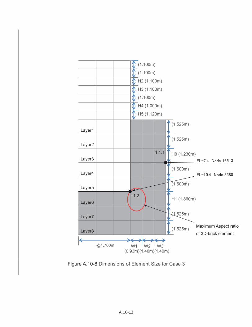
Figure A.10-8 Dimensions of Element Size for Case 3
Layer1
Layer2
Layer3 1:1.1
Layer4
Layer5
Layer6 1:2
Layer7
Layer8
Maximum Aspect ratio
of 3D-brick element
@1.700m
(1.525m)
(1.525m)
H0 (1.230m)
(1.500m)
(1.500m)
H1 (1.860m)
(1.525m)
(1.525m)
W1 W2 W3 (0.93m)(1.40m)(1.40m)
(1.100m)
(1.100m)
H2 (1.100m)
H3 (1.100m)
(1.100m)
H4 (1.000m)
H5 (1.120m)

A.10 13
Figure A.10-9 Dimensions of Element Size for Case 4
Layer1
Layer2
Layer3 1:1.3
Layer4
Layer5
Layer6 1:1.3
Layer7
Layer8
Maximum Aspect ratio
of 3D-brick element
@1.700m
(1.525m)
(1.525m)
H0 (1.230m)
(1.500m)
(1.500m)
H1 (1.860m)
(1.525m)
(1.525m)
W1 W2 W3 (0.62m)(1.555m)(1.555m)
(1.100m)
(1.100m)
H2 (1.100m)
H3 (1.100m)
(1.100m)
H4 (1.000m)
H5 (1.120m)

A.10 14
Figure A.10-10 Dimensions of Element Size for Case 5
Layer1
Layer2
Layer3 1:1.3
Layer4
Layer5
Layer6 1:4
Layer7
Layer8
Maximum Aspect ratio
of 3D-brick element
@1.700m
(1.525m)
(1.525m)
H0 (1.230m)
(1.500m)
(1.500m)
H1 (1.860m)
(1.525m)
(1.525m)
W1 W2 W3 (0.465m)(1.633m)(1.633m)
(1.100m)
(1.100m)
H2 (1.100m)
H3 (1.100m)
(1.100m)
H4 (1.000m)
H5 (1.120m)

A.10 15
Figure A.10-11 Dimensions of Element Size for Case 6
1:1.3
1:1.5
Layer1
Layer2
Layer3
Layer4
Layer5
Layer6
Layer7
Layer8
Maximum Aspect ratio
of 3D-thin shell element
@1.700m
(1.300m)
H2 (1.300m)
H3 (1.300m)
(1.300m)
H4 (1.300m)
H5 (1.120m)
W1 W2 (1.865m)(1.865m)
(1.427m)
(1.426m)
H0 (1.427m)
(1.500m)
(1.500m)
H1 (1.637m)
(1.636m)
(1.637m)

A.10 16
Figure A.10-12 Dimensions of Element Size for Case 7
1:4
1:1.7
Layer1
Layer2
Layer3
Layer4
Layer5
Layer6
Layer7
Layer8
Maximum Aspect ratio
of 3D-thin shell element
@1.700m
(1.100m)
(1.100m)
H2 (0.425m)
H3 (1.775m)
(1.100m)
H4 (1.000m)
H5 (1.120m)
W1 W2 (1.865m)(1.865m)
(1.427m)
(1.426m)
H0 (1.427m)
(1.500m)
(1.500m)
H1 (1.637m)
(1.636m)
(1.637m)

A.10 17
Figure A.10-13 Acceleration Response Spectrum in X-Dir. at Top stick (Node 6) for Cases 1 to 5
Figure A.10-14 Acceleration Response Spectrum in Y-Dir. at Top stick (Node 6) for Cases 1 to 5
0.0
2.0
4.0
6.0
8.0
ACCE
LERA
TIONRE
SPONSE
SPECTR
A(g)
FREQUENCY (Hz)
Node 6 in X Dir.(Aspect Ratio=1:1.3)
Node 6 in X Dir.(Aspect Ratio=1:1.5)
Node 6 in X Dir.(Aspect Ratio=1:2)
Node 6 in X Dir.(Aspect Ratio=1:3)
Node 6 in X Dir.(Aspect Ratio=1:4)
0.0
2.0
4.0
6.0
8.0
ACCE
LERA
TIONRE
SPONSE
SPECTR
A(g)
FREQUENCY (Hz)
Node 6 in Y Dir.(Aspect Ratio=1:1.3)
Node 6 in Y Dir.(Aspect Ratio=1:1.5)
Node 6 in Y Dir.(Aspect Ratio=1:2)
Node 6 in Y Dir.(Aspect Ratio=1:3)
Node 6 in Y Dir.(Aspect Ratio=1:4)

A.10 18
Figure A.10-15 Acceleration Response Spectrum in Z-Dir. at Top stick (Node 6) for Cases 1 to 5
Figure A.10-16 Acceleration Response Spectrum in X-Dir. at Basemat (Node 2) for Cases 1 to 5
0.0
2.0
4.0
6.0
8.0
ACCE
LERA
TIONRE
SPONSE
SPECTR
A(g)
FREQUENCY (Hz)
Node 6 in Z Dir.(Aspect Ratio=1:1.3)
Node 6 in Z Dir.(Aspect Ratio=1:1.5)
Node 6 in Z Dir.(Aspect Ratio=1:2)
Node 6 in Z Dir.(Aspect Ratio=1:3)
Node 6 in Z Dir.(Aspect Ratio=1:4)
0.0
2.0
4.0
6.0
8.0
ACCE
LERA
TIONRE
SPONSE
SPECTR
A(g)
FREQUENCY (Hz)
Node 2 in X Dir.(Aspect Ratio=1:1.3)
Node 2 in X Dir.(Aspect Ratio=1:1.5)
Node 2 in X Dir.(Aspect Ratio=1:2)
Node 2 in X Dir.(Aspect Ratio=1:3)
Node 2 in X Dir.(Aspect Ratio=1:4)

A.10 19
Figure A.10-17 Acceleration Response Spectrum in Y-Dir. at Basemat (Node 2) for Cases 1 to 5
Figure A.10-18 Acceleration Response Spectrum in Z-Dir. at Basemat (Node 2) for Cases 1 to 5
0.0
2.0
4.0
6.0
8.0
ACCE
LERA
TIONRE
SPONSE
SPECTR
A(g)
FREQUENCY (Hz)
Node 2 in Y Dir.(Aspect Ratio=1:1.3)
Node 2 in Y Dir.(Aspect Ratio=1:1.5)
Node 2 in Y Dir.(Aspect Ratio=1:2)
Node 2 in Y Dir.(Aspect Ratio=1:3)
Node 2 in Y Dir.(Aspect Ratio=1:4)
0.0
2.0
4.0
6.0
8.0
ACCE
LERA
TIONRE
SPONSE
SPECTR
A(g)
FREQUENCY (Hz)
Node 2 in Z Dir.(Aspect Ratio=1:1.3)
Node 2 in Z Dir.(Aspect Ratio=1:1.5)
Node 2 in Z Dir.(Aspect Ratio=1:2)
Node 2 in Z Dir.(Aspect Ratio=1:3)
Node 2 in Z Dir.(Aspect Ratio=1:4)
A.10 20
Figure A.10-19 Acceleration Response Spectrum in X-Dir. at Top stick (Node 6) for Cases 2,6 and 7
Figure A.10-20 Acceleration Response Spectrum in Y-Dir. at Top stick (Node 6) for Cases 2,6 and 7
0.0
2.0
4.0
6.0
8.0
ACCE
LERA
TIONRE
SPONSE
SPEC
TRA(g)
FREQUENCY (Hz)
Node 6 in X Dir.(Aspect Ratio=1:1.7)
Node 6 in X Dir.(Aspect Ratio=1:1.5)
Node 6 in X Dir.(Aspect Ratio=1:4)
0.0
2.0
4.0
6.0
8.0
ACCELERA
TIONRE
SPONSE
SPEC
TRA(g)
FREQUENCY (Hz)
Node 6 in Y Dir.(Aspect Ratio=1:1.7)
Node 6 in Y Dir.(Aspect Ratio=1:1.5)
Node 6 in Y Dir.(Aspect Ratio=1:4)

A.10 21
Figure A.10-21 Acceleration Response Spectrum in Z-Dir. at Top stick (Node 6) for Cases 2,6 and 7
Figure A.10-22 Acceleration Response Spectrum in X-Dir. at Basemat (Node 2) for Cases 2,6 and 7
0.0
2.0
4.0
6.0
8.0
ACCE
LERA
TIONRE
SPONSE
SPECTR
A(g)
FREQUENCY (Hz)
Node 6 in Z Dir.(Aspect Ratio=1:1.7)
Node 6 in Z Dir.(Aspect Ratio=1:1.5)
Node 6 in Z Dir.(Aspect Ratio=1:4)
0.0
2.0
4.0
6.0
8.0
ACCE
LERA
TIONRE
SPONSE
SPECTR
A(g)
FREQUENCY (Hz)
Node 2 in X Dir.(Aspect Ratio=1:1.7)
Node 2 in X Dir.(Aspect Ratio=1:1.5)
Node 2 in X Dir.(Aspect Ratio=1:4)

A.10 22
Figure A.10-23 Acceleration Response Spectrum in Y-Dir. at Basemat (Node 2) for Cases 2,6 and 7
Figure A.10-24 Acceleration Response Spectrum in Z-Dir. at Basemat (Node 2) for Cases 2,6 and 7
0.0
2.0
4.0
6.0
8.0
ACCELERA
TIONRE
SPONSE
SPEC
TRA(g)
FREQUENCY (Hz)
Node 2 in Y Dir.(Aspect Ratio=1:1.7)
Node 2 in Y Dir.(Aspect Ratio=1:1.5)
Node 2 in Y Dir.(Aspect Ratio=1:4)
0.0
2.0
4.0
6.0
8.0
ACCE
LERA
TIONRE
SPONSE
SPECTR
A(g)
FREQUENCY (Hz)
Node 2 in Z Dir.(Aspect Ratio=1:1.7)
Node 2 in Z Dir.(Aspect Ratio=1:1.5)
Node 2 in Z Dir.(Aspect Ratio=1:4)

A.10 23
Figure A.10-25 Acceleration Response Spectrum in X-Dir. at Node 1170 and 1234 for Cases 6 and 7
Figure A.10-26 Acceleration Response Spectrum in X-Dir.
at Node 1426 for Cases 2, 6 and 7
0.0
1.0
2.0
3.0
4.0
5.0
0.1 1.0 10.0 100.0
ACCELERA
TIONRE
SPONSE
SPEC
TRA(g)
FREQUENCY(Hz)
Node 1170 in X Dir.(Aspect Ratio=1:1.5)
Node 1234 in X Dir.(Aspect Ratio=1:4)
0.0
1.0
2.0
3.0
4.0
5.0
0.1 1.0 10.0 100.0
ACCELERA
TIONRE
SPONSE
SPECTR
A(g)
FREQUENCY(Hz)
Node 1426 in X Dir.(Aspect Ratio=1:1.7)
Node 1426 in X Dir.(Aspect Ratio=1:1.5)
Node 1426 in X Dir.(Aspect Ratio=1:1.4)

A.10 24
Figure A.10-27 Acceleration Response Spectrum in X-Dir.
at Node 8380 for Cases 1 to 5
Figure A.10-28 Acceleration Response Spectrum in X-Dir.
at Node 16488 and 16513 for Cases 1 to 5
0.0
1.0
2.0
3.0
4.0
5.0
0.1 1.0 10.0 100.0
ACCELERA
TIONRE
SPONSE
SPECTR
A(g)
FREQUENCY(Hz)
Node 8380 in X Dir.(Aspect Ratio=1:1.3)
Node 8380 in X Dir.(Aspect Ratio=1:1.5)
Node 8380 in X Dir.(Aspect Ratio=1:2)
Node 8380 in X Dir.(Aspect Ratio=1:3)
Node 8380 in X Dir.(Aspect Ratio=1:4)
0.0
1.0
2.0
3.0
4.0
5.0
0.1 1.0 10.0 100.0
ACCELERA
TIONRE
SPONSE
SPEC
TRA(g)
FREQUENCY(Hz)
Node 16488 in X Dir.(Aspect Ratio=1:1.3)
Node 16513 in X Dir.(Aspect Ratio=1:1.5)
Node 16513 in X Dir.(Aspect Ratio=1:2)
Node 16513 in X Dir.(Aspect Ratio=1:3)
Node 16513 in X Dir.(Aspect Ratio=1:4)

A.10 25
Figure A.10-29 Acceleration Response Spectrum in Y-Dir.
at Node 1170 and 1234 for Cases 6 and 7
Figure A.10-30 Acceleration Response Spectrum in Y-Dir.
at Node 1426 for Cases 2, 6 and 7
0.0
1.0
2.0
3.0
4.0
5.0
0.1 1.0 10.0 100.0
ACCELERA
TIONRE
SPONSE
SPEC
TRA(g)
FREQUENCY(Hz)
Node 1170 in Y Dir.(Aspect Ratio=1:1.5)
Node 1234 in Y Dir.(Aspect Ratio=1:4)
0.0
1.0
2.0
3.0
4.0
5.0
0.1 1.0 10.0 100.0
ACCELERA
TIONRE
SPONSE
SPECTR
A(g)
FREQUENCY(Hz)
Node 1426 in Y Dir.(Aspect Ratio=1:1.7)
Node 1426 in Y Dir.(Aspect Ratio=1:1.5)
Node 1426 in Y Dir.(Aspect Ratio=1:4)

A.10 26
Figure A.10-31 Acceleration Response Spectrum in Y-Dir. at Node 8380 for Cases 1 to 5
Figure A.10-32 Acceleration Response Spectrum in Y-Dir.
at Node 16488 and16513 for Cases 1 to 5
0.0
1.0
2.0
3.0
4.0
5.0
0.1 1.0 10.0 100.0
ACCELERA
TIONRE
SPONSE
SPECTR
A(g)
FREQUENCY(Hz)
Node 8380 in Y Dir.(Aspect Ratio=1:1.3)
Node 8380 in Y Dir.(Aspect Ratio=1:1.5)
Node 8380 in Y Dir.(Aspect Ratio=1:2)
Node 8380 in Y Dir.(Aspect Ratio=1:3)
Node 8380 in Y Dir.(Aspect Ratio=1:4)
0.0
1.0
2.0
3.0
4.0
5.0
0.1 1.0 10.0 100.0
ACCELERA
TIONRE
SPONSE
SPEC
TRA(g)
FREQUENCY(Hz)
Node 16488 in Y Dir.(Aspect Ratio=1:1.3)
Node 16513 in Y Dir.(Aspect Ratio=1:1.5)
Node 16513 in Y Dir.(Aspect Ratio=1:1.2)
Node 16513 in Y Dir.(Aspect Ratio=1:3)
Node 16513 in Y Dir.(Aspect Ratio=1:4)

A.10 27
Figure A.10-33 Acceleration Response Spectrum in Z-Dir.
at Node 1170 and 1234 for Cases 6 and 7
Figure A.10-34 Acceleration Response Spectrum in Z-Dir.
at Node 1426 for Cases 2, 6 and 7
0.0
1.0
2.0
3.0
4.0
5.0
0.1 1.0 10.0 100.0
ACCELERA
TIONRE
SPONSE
SPECTR
A(g)
FREQUENCY(Hz)
Node 1170 in Z Dir.(Aspect Ratio=1:1.5)
Node 1234 in Z Dir.(Aspect Ratio=1:4)
0.0
1.0
2.0
3.0
4.0
5.0
0.1 1.0 10.0 100.0
ACCELERA
TIONRE
SPONSE
SPEC
TRA(g)
FREQUENCY(Hz)
Node 1426 in Z Dir.(Aspect Ratio=1:1.3)
Node 1426 in Z Dir.(Aspect Ratio=1:1.5)
Node 1426 in Z Dir.(Aspect Ratio=1:1.4)

A.10 28
Figure A.10-35 Acceleration Response Spectrum in Z-Dir. at Node 8380 for Cases 1 to 5
Figure A.10-36 Acceleration Response Spectrum in Z-Dir.
at Node 16488 and 16513 for Cases 1 to 5
0.0
1.0
2.0
3.0
4.0
5.0
0.1 1.0 10.0 100.0
ACCELERA
TIONRE
SPONSE
SPECTR
A(g)
FREQUENCY(Hz)
Node 8380 in Z Dir.(Aspect Ratio=1:1.2)
Node 8380 in Z Dir.(Aspect Ratio=1:1.5)
Node 8380 in Z Dir.(Aspect Ratio=1:2)
Node 8380 in Z Dir.(Aspect Ratio=1:3)
Node 8380 in Z Dir.(Aspect Ratio=1:4)
0.0
1.0
2.0
3.0
4.0
5.0
0.1 1.0 10.0 100.0
ACCELERA
TIONRE
SPONSE
SPECTR
A(g)
FREQUENCY(Hz)
Node 16488 in Z Dir.(Aspect Ratio=1:1.3)
Node 16513 in Z Dir.(Aspect Ratio=1:1.5)
Node 16513 in Z Dir.(Aspect Ratio=1:2)
Node 16513 in Z Dir.(Aspect Ratio=1:3)
Node 16513 in Z Dir.(Aspect Ratio=1:4)