Perspective Factorization Methods for Euclidean

Reconstruction

Mei Han Takeo Kanade

August 1999

CMU-RI-TR-99-22

The Robotics InstituteCarnegie Mellon University

Pittsburgh, PA 15213

@1999 Carnegie Mellon University

Abstract

In this paper we describe a factorization-based method for Euclidean recon-struction with a perspective camera model. It iteratively recovers shape andmotion by weak perspective factorization method and converges to a per-spective model. We discuss the approach of solving the reversal shape am-biguity and analyze its convergence. We also present a factorization-basedmethod to recover Euclidean shape and camera focal lengths from multiplesemi-calibrated perspective views. The focal lengths are the only unknownintrinsic camera parameters and they are not necessarily constant among dif-ferent views. The method �rst performs projective reconstruction by usingiterative factorization, then converts the projective solution to the Euclideanone and generates the focal lengths by using normalization constraints. Thismethod introduces a new way of camera self-calibration. Experiments ofshape reconstruction and camera calibration are presented. We design a cri-terion called back projection compactness to quantify the calibration results.It measures the radius of the minimum sphere through which all back projec-tion rays from the image positions of the same object point pass. We discussthe validity of this criterion and use it to compare the calibration results withother methods.

Keywords: structure from motion, calibration, computer vision

1 Introduction

The problem of recovering shape and motion from an image sequence hasreceived a lot of attention. Previous approaches include recursive methods(e.g., [12]) and batch methods (e.g., [17] and [14]). The factorization method,�rst developed by Tomasi and Kanade [17], recovers the shape of the objectand the motion of the camera from a sequence of images given tracking ofmany feature points. This method achieves its robustness and accuracy byapplying the singular value decomposition (SVD) to a large number of im-ages and feature points. However, it assumes the orthographic projection andknown intrinsic parameters. Poelman and Kanade [14] presented a factoriza-tion method based on the weak perspective and paraperspective projectionmodels assuming known intrinsic parameters. They also used the result fromthe paraperspective method as an initial value of non-linear optimizationprocess to recover Euclidean shape and motion under a perspective cameramodel.

In this paper we �rst describe a perspective factorization method for Eu-clidean reconstruction. It iteratively recovers shape and motion by weak per-spective factorization method and converges to a perspective model. Com-pared with Poelman and Kanade's method, we do not apply non-linear opti-mization which is computation intensive and converges very slowly if startedfar from the true solution. In our method we solve the reconstruction prob-lem in a quasi linear way by taking advantage of the lower order projectionapproximation (like weak perspective) factorization methods. We also dis-cuss the approach of solving the reversal shape ambiguity and analyze itsconvergence.

Secondly, we deal with the problem of recovering Euclidean shape andcamera calibration simultaneously. Given tracking of feature points, ourfactorization-based method recovers the shape of the object, the motion ofthe camera (i.e., positions and orientations of multiple cameras), and focallengths of cameras. We assume other intrinsic parameters are known or canbe taken as generic values. The method �rst performs projective reconstruc-tion by using iterative factorization, then converts the projective solution tothe Euclidean one and generates the focal lengths by using normalizationconstraints. This method introduces a new way of camera self-calibration.Experiments of shape reconstruction and camera calibration are presented.

We design a criterion called back projection compactness to quantify thecalibration results. It measures the radius of the minimum sphere through

1

which all back projection rays from the image positions of the same objectpoint pass. We discuss the validity of this criterion and use it to comparethe calibration results with other methods.

2 Related Work

Tomasi and Kanade [17] developed a robust and e�cient method to recoverthe shape of the object and the motion of the camera from a sequence ofimages, called the factorization method. Like most traditional methods, thefactorization method requires that the image positions of point features �rstbe tracked throughout the stream. This method processes the feature tra-jectory information using the singular value decomposition (SVD) to thesefeature points. However, the method's applicability is somewhat limited dueto its use of an orthographic projection model. Poelman and Kanade [14]presented a factorization method based on the weak perspective and para-perspective projection models assuming known intrinsic parameters. Theyalso used the result from the paraperspective method as an initial value ofnon-linear optimization process to recover Euclidean shape and motion underperspective camera models. The non-linear process is computation intensiveand requires good initial values to converge.

Szeliski and Kang [16] used a non-linear least squares technique for per-spective projection models. Their method can work on partial or uncertainfeature tracks. They also initialized the alternative representation of focallength as scale factor and perspective distortion factor which improved sta-bility and accuracy of recovery results.

Yu [21] presented a new approach based on a higher-order approximationof perspective projection by using Taylor expansion of depth. A methodcalled \back-projection" is used to determine the Euclidean shape and mo-tion instead of normalization constraints. This method approximates theperspective projection e�ects by higher order Taylor expansion which doesnot solve the projective depth literally. The accuracy of the approximationdepends on the order of Taylor expansion and the computation increasesexponentially as the order increases.

Christy and Horaud [1] [2] described a method for solving the Euclideanreconstruction problem with a perspective camera model by incrementallyperforming Euclidean reconstruction with either a weak or a paraperspectivecamera model. Given a sequence of images with a calibrated camera, this

2

method converges in a few iterations, is computationally e�cient. To dealwith the reversal shape ambiguity problem, the method keeps two shapes (theshape and its mirror shape) to re�ne and postpones the decision between thetwo shapes at the end. At each iteration, weak or paraperspective methodgenerates two shapes with sign ambiguity for every one of the two shapesbeing kept. The method checks the consistency of the two newly generatedambiguous shapes with the current shape being re�ned and chooses the moreconsistent one as the re�ned shape. In this way the method avoids theexplosion of the number of solutions. The drawback is that it still keeps twolines of shapes to converge which doubles the computation cost.

There has been considerable progress on projective reconstruction in thelast few years. One can start with uncalibrated cameras and unknown metricstructure, initially recovering the scene up to an projective transformation [3][13]. Triggs [18] viewed the projective reconstruction as a matter of recover-ing a coherent set of projective depths { projective scale factors that representthe depth information lost during image projection. It is a well-known factthat it is only possible to make reconstruction up to an unknown projectivetransformations when nothing about the intrinsic parameters, extrinsic pa-rameters or the object is known. Thus it is necessary to have some additionalinformation about either the intrinsic parameters, the extrinsic parametersor the object in order to obtain the desired Euclidean reconstruction.

Hartley recovered the Euclidean shape by a global optimization techniqueassuming the intrinsic parameters are constant [5]. In [8] Heyden showed thattheoretically Euclidean reconstruction is possible even when the focal lengthand principal point are unknown and varying. The proof is based on the as-sumption of generic camera motion and known skew and aspect ratio. Theydeveloped a bundle adjustment algorithm to estimate all the unknown pa-rameters, including focal lengths, principle points, camera motion and objectshape. However, if the camera motion is not su�ciently general, then thisis not possible. Pollefeys assumed the focal length as the only varying in-trinsic parameter and presented a linear method to recover focal length [15].Then they used the epipolar geometry to obtain a pair-wise image recti�ca-tion to get the dense correspondence matches based on which the dense 3Dmodel is generated. Maybank and Faugeras [11] gave a detailed discussion ofthe connection between the calibration of a single camera and the epipolartransformation obtained when the camera undergoes a displacement.

Most current reconstruction methods either work only for minimal num-ber of views, or single out a few views for initialization to the multiple views.

3

To achieve robustness and accuracy, it is necessary to uniformly take accountof all the data in all the images like in factorization methods. Triggs pro-posed a projective factorization method in [19] which recovered the projectivedepths by estimating a set of fundamental matrices and epipoles to chain allthe images together. Based on the reconstruction of projective depths, a fac-torization is applied to the rescaled measurement matrix to generate shapeand motion. Strictly speaking, the �rst step which recovers the projectivedepths is not a uniform batch approach.

Heyden [6] [7] presented methods of using subspace multilinear constraintsto perform projective structure from motion. In [6] Heyden proposed aniterative algorithm based on SVD of the projective shape matrices. Thealgorithm is similar to our bilinear projective recovery method while oursperforms SVD on the scaled measurement matrix which is more direct andsimpler.

3 Perspective Factorization Method with Cal-

ibrated Cameras

Assuming the intrinsic parameters of the cameras are known, perspective fac-torization method reconstructs the Euclidean object shape and the cameramotion from the feature points correspondences under a perspective projec-tion model.

3.1 Algorithm description

3.1.1 Perspective projection

We denote by sj = (xj yj zj) a 3D point represented in the world coordinatesystem Cw whose origin is usually chosen at the gravity center of the object.The representations of points in the camera coordinate systems Cc are (Ii �sj + txi Ji � sj + tyi Ki � sj + tzi) where (Ii Ji Ki) are the rotations of the ithcamera represented in Cw and (txi tyi tzi) are the translations.

Assuming the camera intrinsic parameters are known, the relationshipbetween the object points and the image coordinates can be written as:

uij =Ii � sj + txi

Ki � sj + tzi

4

vij =Ji � sj + tyi

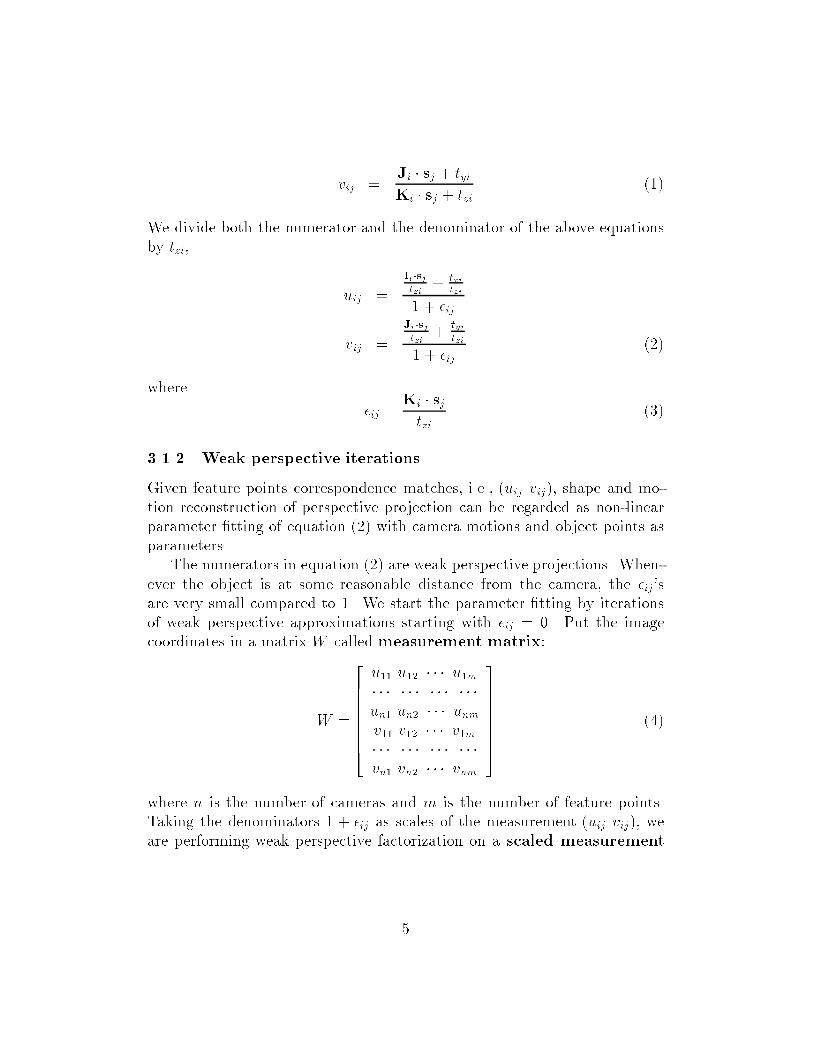
Ki � sj + tzi(1)

We divide both the numerator and the denominator of the above equationsby tzi,

uij =

Ii�sj

tzi+ txi

tzi

1 + �ij

vij =

Ji�sj

tzi+ tyi

tzi

1 + �ij(2)

where

�ij =Ki � sjtzi

(3)

3.1.2 Weak perspective iterations

Given feature points correspondence matches, i.e., (uij vij), shape and mo-tion reconstruction of perspective projection can be regarded as non-linearparameter �tting of equation (2) with camera motions and object points asparameters.

The numerators in equation (2) are weak perspective projections. When-ever the object is at some reasonable distance from the camera, the �ij'sare very small compared to 1. We start the parameter �tting by iterationsof weak perspective approximations starting with �ij = 0. Put the imagecoordinates in a matrix W called measurement matrix:

W =

2666666664

u11 u12 � � � u1m� � � � � � � � � � � �un1 un2 � � � unmv11 v12 � � � v1m� � � � � � � � � � � �vn1 vn2 � � � vnm

3777777775

(4)

where n is the number of cameras and m is the number of feature points.Taking the denominators 1 + �ij as scales of the measurement (uij vij), weare performing weak perspective factorization on a scaled measurement

5

matrix Ws to get motion and shape parameters:

Ws =

2666666664

�11u11 �12u12 � � � �1mu1m� � � � � � � � � � � �

�n1un1 �n2un2 � � � �nmunm�11v11 �12v12 � � � �1mv1m

� � � � � � � � � � � ��n1vn1 �n2vn2 � � � �nmvnm

3777777775

(5)

where �ij = 1+�ij . The current motion parameters are denoted as (I0i J0

i K0

i)and (t0xi t

0

yi t0

zi). The current points are denoted as s0j = (x0j y0

j z0

j). Then weuse these current parameters to generate a new measurement matrix W 0:

W 0 =

2666666664

u011 u0

12 � � � u01m� � � � � � � � � � � �u0n1 u

0

n2 � � � u0nmv011 v

0

12 � � � v01m� � � � � � � � � � � �v0n1 v

0

n2 � � � v0nm

3777777775

(6)

where

u0ij =I0i � s

0

j + t0xiK0

i � s0j + t0zi

v0ij =J0i � s

0

j + t0yi

K0i � s0j + t0zi

(7)

The process of computing the new measurement matrix is equivalent to theback projection process in many non-linear optimization methods. The newmeasurement matrix W 0 provides a criterion to choose between the two am-biguous shapes which are up to an mirror-symmetry transformation and itsdi�erence from the original measurementmatrixW also gives the convergenceerror. Re�ned scales �ij are calculated from the current parameters and anew scaled measurement matrix is generated on which another iteration ofweak perspective factorization is performed. The goal of parameter �tting isto iteratively �nd the scales which make the back projection consistent withthe measurement.

3.1.3 Reconstruction algorithm

The perspective factorization method can be summarized by the followingalgorithm.

6

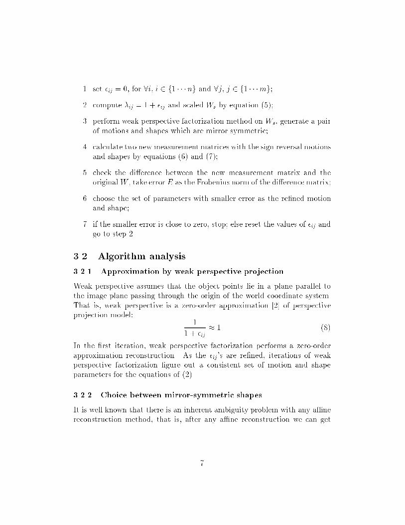
1. set �ij = 0, for 8i, i 2 f1 � � � ng and 8j, j 2 f1 � � �mg;

2. compute �ij = 1 + �ij and scaled Ws by equation (5);

3. perform weak perspective factorization method on Ws, generate a pairof motions and shapes which are mirror symmetric;

4. calculate two new measurementmatrices with the sign reversal motionsand shapes by equations (6) and (7);

5. check the di�erence between the new measurement matrix and theoriginalW , take error E as the Frobenius norm of the di�erence matrix;

6. choose the set of parameters with smaller error as the re�ned motionand shape;

7. if the smaller error is close to zero, stop; else reset the values of �ij andgo to step 2.

3.2 Algorithm analysis

3.2.1 Approximation by weak perspective projection

Weak perspective assumes that the object points lie in a plane parallel tothe image plane passing through the origin of the world coordinate system.That is, weak perspective is a zero-order approximation [2] of perspectiveprojection model:

1

1 + �ij� 1 (8)

In the �rst iteration, weak perspective factorization performs a zero-orderapproximation reconstruction. As the �ij's are re�ned, iterations of weakperspective factorization �gure out a consistent set of motion and shapeparameters for the equations of (2).

3.2.2 Choice between mirror-symmetric shapes

It is well known that there is an inherent ambiguity problem with any a�nereconstruction method, that is, after any a�ne reconstruction we can get

7

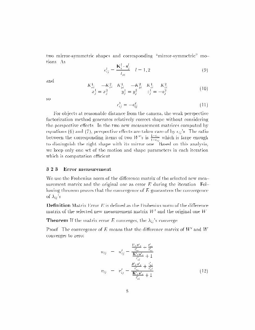
two mirror-symmetric shapes and corresponding \mirror-symmetric" mo-tions. As

�lij =Kl

i � slj

tzil = 1; 2 (9)

andK1

xi = �K2xi K1

yi = �K2yi K1

zi = K2zi

x1j = x2j y1j = y2j z1j = �z2j(10)

so�1ij = ��2ij (11)

For objects at reasonable distance from the camera, the weak perspectivefactorization method generates relatively correct shape without consideringthe perspective e�ects. In the two new measurement matrices computed byequations (6) and (7), perspective e�ects are taken care of by �ij's. The ratiobetween the corresponding items of two W 0's is 1+�ij

1��ijwhich is large enough

to distinguish the right shape with its mirror one. Based on this analysis,we keep only one set of the motion and shape parameters in each iterationwhich is computation e�cient.

3.2.3 Error measurement

We use the Frobenius norm of the di�erence matrix of the selected new mea-surement matrix and the original one as error E during the iteration. Fol-lowing theorem proves that the convergence of E guarantees the convergenceof �ij 's.

De�nitionMatrix Error E is de�ned as the Frobenius norm of the di�erencematrix of the selected new measurement matrix W 0 and the original one W .

Theorem If the matrix error E converges, the �ij's converge.

Proof. The convergence of E means that the di�erence matrix of W 0 and Wconverges to zero:

uij = u0ij =

I0i�s0j

t0zi

+t0xit0zi

K0i�s

0j

t0zi

+ 1

vij = v0ij =

J0

i�s0

j

t0zi

+t0yi

t0zi

K0i�s

0j

t0zi

+ 1(12)

8

Currently,

�ij =K0

i � s0

j

t0zi+ 1 (13)

Using the above �ij 's to get the scaled measurement matrix on which aniteration of weak perspective factorization is performed, from equation (12)it is obvious that this iteration generates the same motion and shape as thelast iteration. Therefore, �ij's stay constant according to equation (13), i.e.,�ij 's converge.

4 Perspective Factorization Method with Un-

known Focal Lengths

Assuming the cameras are semi-calibrated, i.e., the intrinsic parameters areknown or taken as generic values (like skew = 0, principle point is in themiddle of the image) except the focal lengths, the perspective factorizationmethod reconstructs the Euclidean object shape, the camera motion and thefocal lengths given the feature points correspondences under a perspectiveprojection model. This method �rst recovers projective shape and motion byiterative factorization and projective depths re�nement, then reconstructs theEuclidean shape, the camera motion and the focal lengths by normalizationprocess.

4.1 Projective Reconstruction

Suppose there are n perspective cameras: Pi, i = 1 � � � n and m object pointsxj, j = 1 � � �m represented by homogeneous coordinates. The image coordi-nates are represented by (uij vij). Using the symbol � to denote equality upto a scale, the following holds

264 uijvij1

375 � Pixj (14)

or

�ij

264 uijvij1

375 = Pixj (15)

9

where �ij is a non-zero scale factor which is commonly called projective depth.The equivalent matrix form is:

Ws =

2666666666664

�11

264 u11v111

375 � � � �1m

264 u1mv1m1

375

......

...

�n1

264 un1vn11

375 � � � �nm

264 unmvnm1

375

3777777777775=

2664P1...Pn

3775 [x1 � � � xm] (16)

Ws is the scaled measurement matrix. Quite similar to the iterativealgorithm described in the previous section, projective factorization methodis summarized as:

1. set �ij = 1, for 8i, i 2 f1 � � � ng and 8j, j 2 f1 � � �mg;

2. get the scaled measurement matrix Ws by equation (16);

3. perform rank4 factorization method on Ws, generate projective shapeand motion;

4. reset the values of �ij = P(3)i xj where P

(3)i denotes the third row of the

projection matrix Pi;

5. if �ij's are the same as the previous iteration, stop; else go to step 2.

The goal of the projective reconstruction process is to estimate the valuesof the projective depths (�ij 's) which make the equation (16) consistent. Thereconstruction results are iteratively improved by back projecting the pro-jective reconstruction of an iteration to re�ne the depth estimates. Triggspointed out in [19] that the iteration turned out to be extremely stable evenstarting with arbitrary initial depths. In practice we use rough knowledge ofthe focal lengths and the perspective factorization method with calibratedcameras to get the initial values of �ij 's which drastically improve the con-vergence speed.

10

4.2 Normalization

The factorization of equation (16) is only determined up to a linear transfor-mation B4�4:

Ws = P̂ X̂ = P̂BB�1X̂ = PX (17)

where P = P̂B and X = B�1X̂. P̂ and X̂ are referred to as the projectivemotion and the projective shape. Any non-singular 4� 4 matrix B could beinserted between P̂ and X̂ to get another pair of motion and shape. With theassumption that the focal lengths are the only unknown intrinsic parameters,we have the projective motion matrix Pi,

Pi � Ki [Rijti] (18)

where

Ki =

264 fi 0 0

0 fi 00 0 1

375 Ri =

264 iTijTikTi

375 ti =

264 txityitzi

375

The upper triangular calibration matrix Ki encodes the intrinsic parametersof the ith camera: fi represents the focal length, the principal point is (0; 0)and the aspect ratio is 1. Ri is the ith rotation matrix with ii, ji and ki

denoting the rotation axes. ti is the ith translation vector. CombiningEquation (18) for i = 1 � � � n into one matrix equation, we get,

P = [M jT ] (19)

where

M = [mx1 my1 mz1 � � � mxn myn mzn]T

T = [Tx1 Ty1 Tz1 � � � Txn Tyn Tzn]T

and

mxi = �ifiii myi = �ifiji mzi = �iki

Txi = �ifitxi Tyi = �ifityi Tzi = �itzi(20)

The shape matrix is represented by:

X �

"S

1

#(21)

11

whereS = [s1 s2 � � � sm]

and

sj = [xj yj zj]T

xj =h�js

Tj �j

iTWe put the origin of the world coordinate system at the center of gravity ofthe scaled object points to enforce

mXj=1

�jsj = 0 (22)

We get,

mXj=1

�ijuij =mXj=1

(mxi��jsj+�jTxi) =mxi �mXj=1

�jsj+TximXj=1

�j = Txi

mXj=1

�j (23)

Similarly,mXj=1

�ijvij = Tyi

mXj=1

�j

mXj=1

�ij = Tzi

mXj=1

�j (24)

De�ne the 4� 4 projective transformation H as:

H = [AjB] (25)

where A is 4� 3 and B is 4 � 1.Since P = P̂H,

[M jT ] = P̂ [AjB] (26)

we have,Txi = P̂xiB Tyi = P̂yiB Tzi = P̂ziB (27)

From Equations (23) and (24) we know,

Txi

Tzi=

Pmj=1 �ijuijPmj=1 �j

Tyi

Tzi=

Pmj=1 �ijvijPmj=1 �j

(28)

we set up 2n linear equations of the 4 unknown elements of the matrix B.Linear least squares solutions are then computed.

12

As mxi, myi and mzi are scaled rotation axes, we get the following con-straints from Equation (20):

jmxij2 = jmyij

2

mxi �myi = 0mxi �mzi = 0myi �mzi = 0

We can add one more constraint assuming �1 = 1:

jmz1j2 = 1 (29)

The above constraints are linear constraints on MMT. Since

MMT = P̂AATP̂T (30)

Totally we have 4n + 1 linear equations of the 10 unknown elements of thesymmetric 4�4 matrix Q = AAT. Least squares solutions are computed, wethen get the matrix A from Q by rank3 matrix decomposition.

4.3 Reconstruction of shape, motion and focal lengths

Once the matrix A has been found, the projective transformation is [AjB].The shape is computed as X = H�1X̂ and the motion matrix as P = P̂H.We �rst compute the scales �i:

�i = jmzij (31)

We then compute the focal lengths as

fi =jmxij+ jmyij

2�i(32)

Therefore, the motion parameters are

ii =mxi

�ifiji =

myi

�ifiki =

mzi

�i

txi =Txi�ifi

tyi =Tyi

�ifitzi =

Tzi�i

(33)

13

5 Applications

5.1 Scene Reconstruction

The perspective factorization method described in section 3 provides an ef-�cient and robust way to recover the object shape and the camera motionunder a perspective projection model. It takes care of the perspective ef-fects by incremental reconstruction using the weak perspective factorizationmethods. The method assumes the intrinsic parameters are known and thefeature points trajectories in image sequences are given. In this section weapply the perspective factorization method with calibrated cameras on in-door and outdoor scenes, analyze the results and compare with non-linearoptimization approaches.

5.1.1 LED reconstruction

We take the data at the virtualized reality lab. The setup includes a bar ofLEDs which moves around and works as object points (we have 232 featurepoints), and 51 cameras arranged in a dome above the LEDs. Tsai's approach[20] is used to calibrate intrinsic and extrinsic camera parameters. In thisexperiment we use intrinsic parameters calibrated by Tsai's method as knownvalues. The perspective factorization method described in section 3 is appliedon the feature points correspondences in 51 images.

� perspective e�ects

Figure 1(a) shows the recovered object by the weak perspective factor-ization method. The distortions are obvious which are caused by theapproximation of perspective projection with weak perspective projec-tion. Figure 1(b) gives the recovered object by the perspective factor-ization method which takes care of the perspective e�ects by iterativeweak perspective reconstruction.

� reconstruction result

The reconstruction results include the object shape (LEDs positions)and the camera extrinsic parameters which are the camera orientationsand locations. The result is shown in �gure 2. Figure 2(a) is the topview and (b) is the side view. Each camera is represented by its threeaxes where red, green and blue denoting x, y and z axis respectively.The intersections of the axes are the locations of the cameras.

14

(a) (b)

Figure 1: (a) Weak perspective (b) perspective reconstruction of LED posi-tions.

(a) (b)

Figure 2: (a) Top view (b) side view of the LED reconstruction result. Redpoints denote the recovered LED positions. Red, green and blue lines denotethe recovered x, y and z axes of the cameras.

15

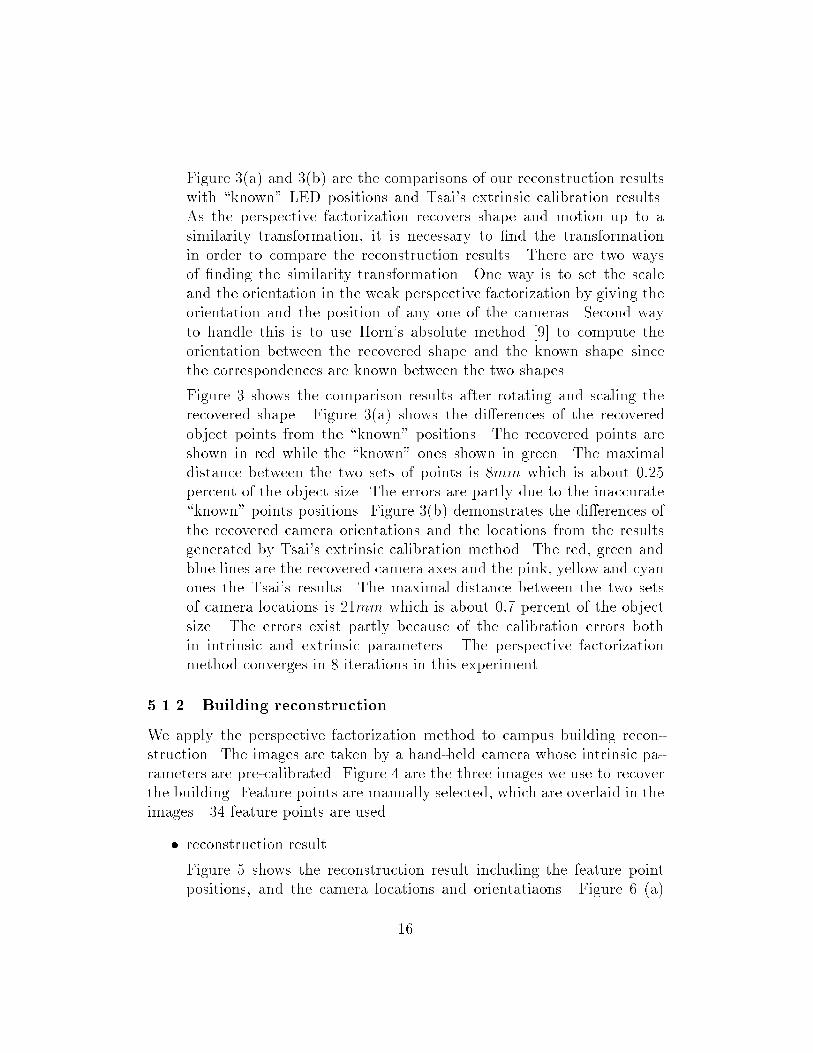
Figure 3(a) and 3(b) are the comparisons of our reconstruction resultswith \known" LED positions and Tsai's extrinsic calibration results.As the perspective factorization recovers shape and motion up to asimilarity transformation, it is necessary to �nd the transformationin order to compare the reconstruction results. There are two waysof �nding the similarity transformation. One way is to set the scaleand the orientation in the weak perspective factorization by giving theorientation and the position of any one of the cameras. Second wayto handle this is to use Horn's absolute method [9] to compute theorientation between the recovered shape and the known shape sincethe correspondences are known between the two shapes.

Figure 3 shows the comparison results after rotating and scaling therecovered shape. Figure 3(a) shows the di�erences of the recoveredobject points from the \known" positions. The recovered points areshown in red while the \known" ones shown in green. The maximaldistance between the two sets of points is 8mm which is about 0:25percent of the object size. The errors are partly due to the inaccurate\known" points positions. Figure 3(b) demonstrates the di�erences ofthe recovered camera orientations and the locations from the resultsgenerated by Tsai's extrinsic calibration method. The red, green andblue lines are the recovered camera axes and the pink, yellow and cyanones the Tsai's results. The maximal distance between the two setsof camera locations is 21mm which is about 0:7 percent of the objectsize. The errors exist partly because of the calibration errors bothin intrinsic and extrinsic parameters. The perspective factorizationmethod converges in 8 iterations in this experiment.

5.1.2 Building reconstruction

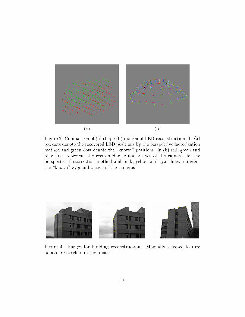
We apply the perspective factorization method to campus building recon-struction. The images are taken by a hand-held camera whose intrinsic pa-rameters are pre-calibrated. Figure 4 are the three images we use to recoverthe building. Feature points are manually selected, which are overlaid in theimages . 34 feature points are used.

� reconstruction result

Figure 5 shows the reconstruction result including the feature pointpositions, and the camera locations and orientatiaons. Figure 6 (a)

16

(a) (b)

Figure 3: Comparison of (a) shape (b) motion of LED reconstruction. In (a)red dots denote the recovered LED positions by the perspective factorizationmethod and green dots denote the \known" positions. In (b) red, green andblue lines represent the recovered x, y and z axes of the cameras by theperspective factorization method and pink, yellow and cyan lines representthe \known" x, y and z axes of the cameras.

Figure 4: Images for building reconstruction. Manually selected featurepoints are overlaid in the images.

17

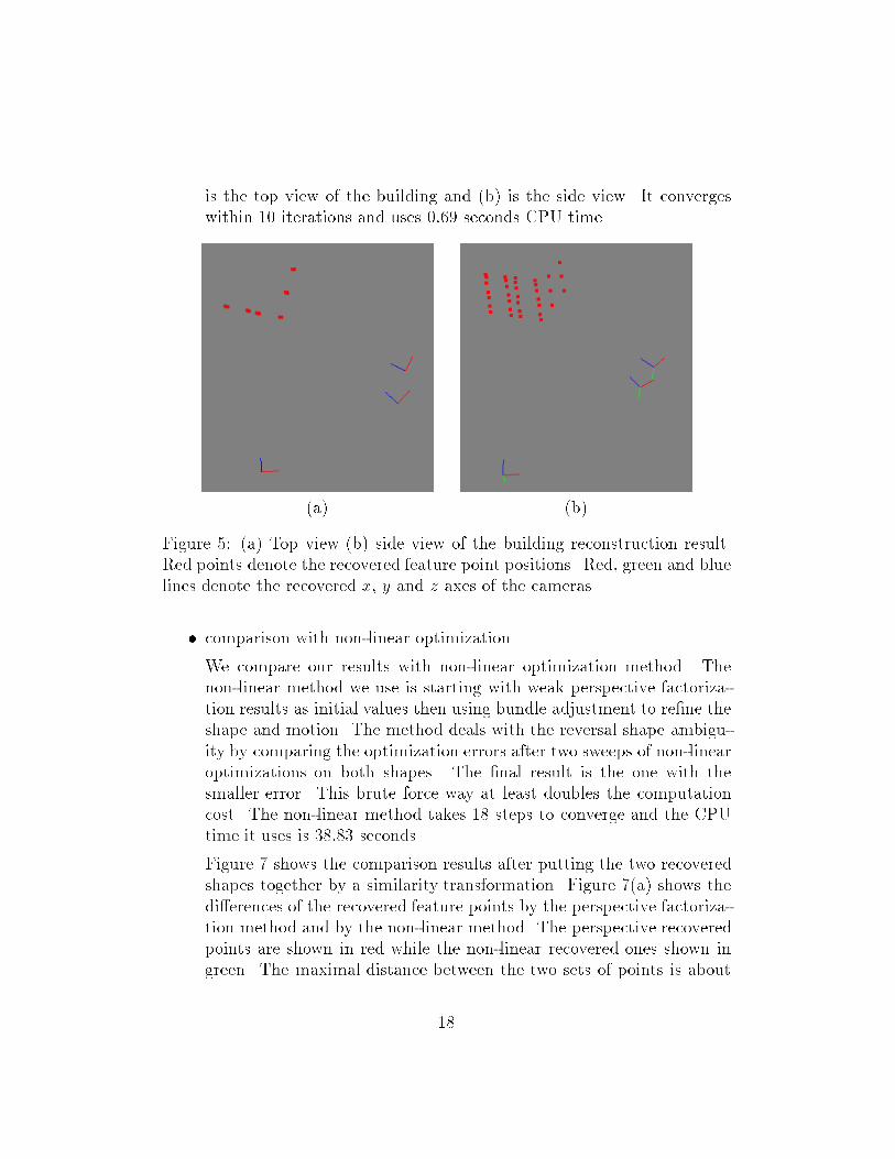
is the top view of the building and (b) is the side view. It convergeswithin 10 iterations and uses 0:69 seconds CPU time.

(a) (b)

Figure 5: (a) Top view (b) side view of the building reconstruction result.Red points denote the recovered feature point positions. Red, green and bluelines denote the recovered x, y and z axes of the cameras.

� comparison with non-linear optimization

We compare our results with non-linear optimization method. Thenon-linear method we use is starting with weak perspective factoriza-tion results as initial values then using bundle adjustment to re�ne theshape and motion. The method deals with the reversal shape ambigu-ity by comparing the optimization errors after two sweeps of non-linearoptimizations on both shapes. The �nal result is the one with thesmaller error. This brute force way at least doubles the computationcost. The non-linear method takes 18 steps to converge and the CPUtime it uses is 38:83 seconds.

Figure 7 shows the comparison results after putting the two recoveredshapes together by a similarity transformation. Figure 7(a) shows thedi�erences of the recovered feature points by the perspective factoriza-tion method and by the non-linear method. The perspective recoveredpoints are shown in red while the non-linear recovered ones shown ingreen. The maximal distance between the two sets of points is about

18

(a) (b)

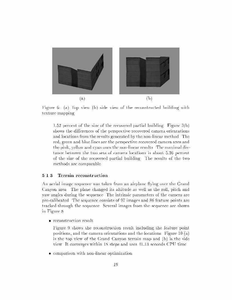
Figure 6: (a) Top view (b) side view of the reconstructed building withtexture mapping.

1:52 percent of the size of the recovered partial building. Figure 7(b)shows the di�erences of the perspective recovered camera orientationsand locations from the results generated by the non-linear method. Thered, green and blue lines are the perspective recovered camera axes andthe pink, yellow and cyan ones the non-linear results. The maximal dis-tance between the two sets of camera locations is about 5:36 percentof the size of the recovered partial building. The results of the twomethods are comparable.

5.1.3 Terrain reconstruction

An aerial image sequence was taken from an airplane ying over the GrandCanyon area. The plane changed its altitude as well as the roll, pitch andyaw angles during the sequence. The intrinsic parameters of the camera arepre-calibrated. The sequence consists of 97 images and 86 feature points aretracked through the sequence. Several images from the sequence are shownin Figure 8.

� reconstruction result

Figure 9 shows the reconstruction result including the feature pointpositions, and the camera orientations and the locations. Figure 10 (a)is the top view of the Grand Canyon terrain map and (b) is the sideview. It converges within 18 steps and uses 41:13 seconds CPU time.

� comparison with non-linear optimization

19

(a) (b)

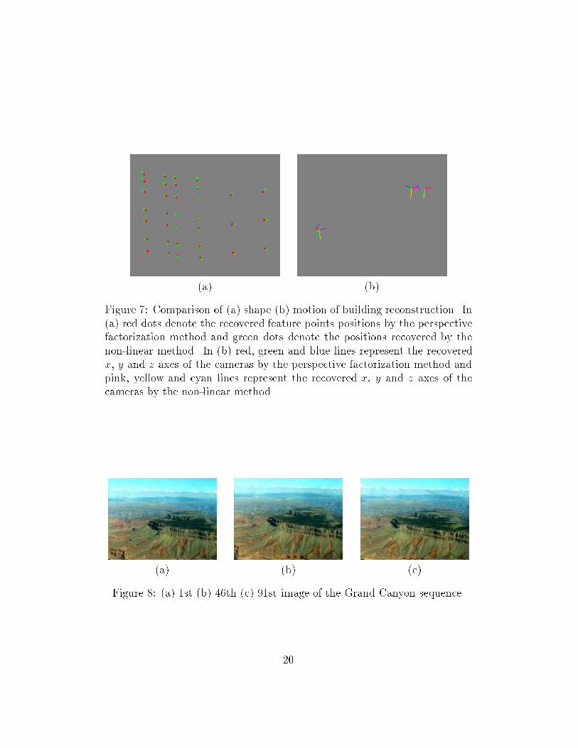
Figure 7: Comparison of (a) shape (b) motion of building reconstruction. In(a) red dots denote the recovered feature points positions by the perspectivefactorization method and green dots denote the positions recovered by thenon-linear method. In (b) red, green and blue lines represent the recoveredx, y and z axes of the cameras by the perspective factorization method andpink, yellow and cyan lines represent the recovered x, y and z axes of thecameras by the non-linear method.

(a) (b) (c)

Figure 8: (a) 1st (b) 46th (c) 91st image of the Grand Canyon sequence.

20

(a) (b)

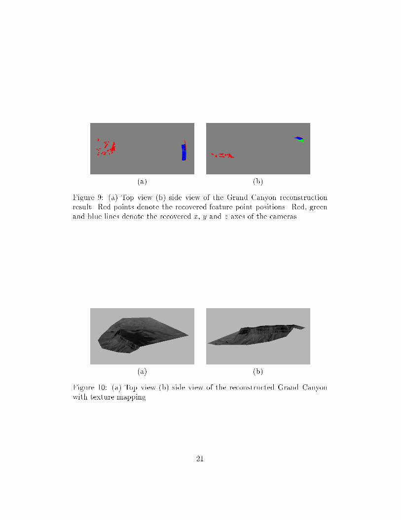
Figure 9: (a) Top view (b) side view of the Grand Canyon reconstructionresult. Red points denote the recovered feature point positions. Red, greenand blue lines denote the recovered x, y and z axes of the cameras.

(a) (b)

Figure 10: (a) Top view (b) side view of the reconstructed Grand Canyonwith texture mapping.

21

We compare our results with the non-linear optimization method aswell. The non-linear method is described in section 5.1.2. It takes 38steps to converge and the CPU time it uses is 9264 seconds.

Figure 11 shows the comparison results after putting the two recoveredshapes together by a similarity transformation. Figure 11(a) shows thedi�erences of the recovered feature points by the perspective factoriza-tion method and by the non-linear method. The perspective recoveredpoints are shown in red while the non-linear recovered ones shown ingreen. The maximal distance between the two sets of points is about5:16 percent of the terrain size of the recovered part. Figure 11(b)shows the di�erences of the perspective recovered camera orientationsand the locations from the results generated by the non-linear method.The red, green and blue lines are the perspective recovered camera axesand the pink, yellow and cyan ones the non-linear results. The max-imal distance between the two sets of camera locations is about 9:12percent of the terrain size of the recovered part.

(a) (b)

Figure 11: Comparison of (a) shape (b) motion of Grand Canyon recon-struction. In (a) red dots denote the recovered feature points positions bythe perspective factorization method and green dots denote the positions re-covered by the non-linear method. In (b) red, green and blue lines representthe recovered x, y and z axes of the cameras by the perspective factorizationmethod and pink, yellow and cyan lines represent the recovered x, y and z

axes of the cameras by the non-linear method.

22

5.2 Self-Calibration

In this section we apply the perspective factorization method with unknownfocal lengths to perform camera self-calibration. Given feature correspon-dences from multiple views, the perspective factorization method recoversfeature points positions, camera locations and orientations as well as camerafocal lengths. We introduce a measurement called back projection compact-ness to compare the calibration results.

5.2.1 Back Projection Compactness

� De�nition

De�nition Back projection compactness is the radius of the minimumsphere through which all back projection rays from the image positionsof the same object point pass.

Back projection compactness measures quantitatively how well the backprojection rays from multiple views converge. The smaller the backprojection compactness is, the better the convergence is.

� Analysis

We design the concept of back projection compactness to measure thecalibration results quantitatively. Calibration is to �nd a set of parame-ters to transfer the object point position to its image coordinates. Howto quantify the calibration results depends on the calibration applica-tions. For applications including structure from motion, image basedrendering, and augmented reality, measuring the compactness of theback projection rays provides a value to quantify how consistent thecamera calibrations are.

In our experiments we compare our self-calibration results with the re-sults of the Tsai's method [20]. For Tsai's method, the object pointpositions in 3D are known and the corresponding image coordinatesare given. The Tsai's method outputs the camera locations and ori-entations as well as the camera intrinsic parameters. Calibration er-ror is caused by the pinhole projection assumption, the inaccurate 3Dpoint positions and the noises of the image measurements. For the per-spective method, only the feature correspondences among the multipleviews are given. It outputs the camera locations and orientations, the

23

object point positions and the camera focal lengths. The perspectivemethod assumes the other intrinsic camera parameters except the fo-cal lengths are generic. Comparing with the Tsai's method, it has thesame error sources from the pinhole camera assumption and the imagemeasurement noises. However, it avoids the inaccuracy of 3D pointpositions which are taken as hard constraints in the Tsai's calibrationmethod.

The goal of the Tsai's method is to make each back projection ray ofthe same point to pass the known 3D position no matter whether itis accurate or not. The perspective factorization method is to makethe back projection rays of the same point to converge to one positionwhich is the recovered object point position. It takes far less constraintsthan the Tsai's method and distributes the reconstruction error to thecalibration results and the recovered shape.

� Algorithm

1. start with a cubic space and divide it into 8 cubes of equal size;

2. for each small cube, compute the distanceD(Ci; Lj) of its centerCi

to every back projection ray Lj, where i = 1 � � � 8 and j = 1 � � �m,m is the number of the cameras;

3. take Di = maxj D(Ci; Lj);

4. choose the cube with the smallest Di, start with this cube anddivide it into 8 cubes of equal size;

5. if the size of the small cube is close to zero, stop, set Ci as thecenter of the sphere and Di as the back projection compactness;else go to step 2.

5.2.2 Experiments

We use the data from the virtualized reality lab for the self-calibration ex-periments. The setup includes a bar of LEDs which moves around and worksas object points, and cameras above the LEDs. Taking the camera intrinsicparameters except the focal lengths as generic (like skew = 0, aspect = 1,the principle point is in the middle of the image), we apply the perspectivefactorization method with unknown focal lengths to the feature points cor-respondences. The outputs of our method include the camera focal lengths,

24

Tsai Persp1 Persp2

Init1 Init2 Init3

max b.p.c. 13.4421 14.3017 15.3703 15.3543 15.5826mean b.p.c. 7.0366 7.1496 8.2491 8.1238 8.3107median b.p.c. 7.1092 7.4294 7.7700 7.6798 7.8294max shapeD || 7.9137 7.4042 7.3847 7.3730max sphereD1 || 8.1359 8.6033 7.7878 7.3842max sphereD2 8.3386 8.4666 8.8477 9.1947 10.0894

Table 1: calibration results

the camera locations and orientations and the object point positions. Tocompare the calibration results, Tsai's approach [20] is used to calibrate theintrinsic and extrinsic camera parameters. The back projection compactnessis calculated from both of the calibration results to quantify the calibrationquality.

In this experiment 223 feature points are used for both of the calibrationmethods. The image number is 51. Table 1 shows the comparison results.Tsai denotes the Tsai's calibration method. Persp1 and Persp2 represent theperspective factorization method with calibrated cameras and with unknownfocal lengths respectively. Init1 and Init2 indicate that the perspective fac-torization method start with the mean value and the median value of the\known" focal lengths from the Tsai's method as initial values. Init3 indi-cate the initial focal lengths are any random numbers within the range (inthis example the range is 365 to 385). It shows that the three results are veryclose which means that the rough knowledge of the focal lengths is enoughfor the perspective calibration method to converge.

The 5 values we compare are the maximal back projection compactnessof 223 object points (denoted as max b.p.c. in Table 1), the mean and themedian values of the back projection compactnesses (denoted as mean b.p.c.

andmedian b.p.c. respectively), the maximal distance of the recovered objectpoints and the \known" object point positions (denoted as max shapeD), themaximal distance of the recovered object points and the back projectioncompactness centers (denoted as max shapeD1) and the maximal distanceof the \known" object point positions and the back projection compactnesscenters (denoted as max shapeD2). The unit representing the distances ismm.

25

6 Discussion

In this paper we �rst describe a perspective factorization method for Eu-clidean reconstruction. It iteratively recovers shape and motion by the weakperspective factorization method and converges to a perspective model. Wesolve the reconstruction problem in a quasi linear way by taking advantage ofthe factorization methods of the lower order projection. Compared with non-linear methods, our method is e�cient and robust. We also present a newway of dealing with the sign ambiguity problem. However, the perspectivefactorization method is conceptually non-linear parameter �tting process.Common problems, such as local minima, still exist. We are working ontheoretical analysis of its convergence.

We successfully recover the shape of the object and the camera calibra-tions simultaneously given tracking of feature points. The factorization-basedmethod �rst performs projective reconstruction by using iterative factoriza-tion, then converts the projective solution to the Euclidean one and generatesthe focal lengths by using normalization constraints. This method intro-duces a new way of camera self-calibration which has various applicationsin autonomous navigation, virtual reality systems and video editing. Theprojective factorization method requires the rough range of focal lengths togenerate an estimate of the projective depths for fast convergence. Accuracyof the calibrations and their e�ects on applications provide further researchtopics.

Freeman [4] described various bilinear model �tting problems in computervision. Koenderink [10] also analyzed the bilinear algebra applied to cameracalibration problem. They both indicated that the self-calibration of per-spective camera is a \hard" problem. We are going to focus on applicationoriented bilinear algebra analysis.

We also design a criterion called back projection compactness to quantifythe calibration results. It measures the radius of the minimumsphere throughwhich all back projection rays of the same object point pass.We use it tocompare the calibration results with other methods. The divide and conqueralgorithm to compute the back projection compactness is e�cient. However,it is still an open problem to prove the algorithm.

26

References

[1] S. Christy and R. Horaud. Euclidean reconstruction: From paraperspec-tive to perspective. In ECCV96, pages II:129{140, 1996.

[2] S. Christy and R. Horaud. Euclidean shape and motion from multipleperspective views by a�ne iterations. PAMI, 18(11):1098{1104, Novem-ber 1996.

[3] O.D. Faugeras. What can be seen in three dimensions with an uncali-brated stereo rig? In ECCV92, pages 563{578, 1992.

[4] W.T. Freeman and J.B. Tenenbaum. Learning bilinear models for twofactor problems in vision. In CVPR97, pages 554{560, 1997.

[5] R.I. Hartley. Euclidean reconstruction from uncalibrated views. InCVPR94, pages 908{912, 1994.

[6] A. Heyden. Projective structure and motion from image sequences usingsubspace methods. In SCIA97, 1997.

[7] A. Heyden. Reduced multilinear constraints: Theory and experiments.IJCV, 30(1):5{26, October 1998.

[8] A. Heyden and K. Astrom. Euclidean reconstruction from image se-quences with varying and unknown focal length and principal point. InCVPR97, pages 438{443, 1997.

[9] B.K.P. Horn. Closed form solutions of absolute orientation using unitquaternions. JOSA-A, 4(4):629{642, April 1987.

[10] J.J. Koenderink and A.J. vanDoorn. The generic bilinear calibration-estimation problem. IJCV, 23(3):217{234, 1997.

[11] S. Maybank and O.D. Faugeras. A theory of self-calibration of a movingcamera. IJCV, 8(2):123{151, August 1992.

[12] P.F. McLauchlan, I.D. Reid, and D.W. Murray. Recursive a�ne struc-ture and motion from image sequences. In ECCV94, volume 1, pages217{224, 1994.

27

[13] R. Mohr, L. Quan, and F. Veillon. Relative 3d reconstruction usingmultiple uncalibrated images. IJRR, 14(6):619{632, December 1995.

[14] C. Poelman and T. Kanade. A paraperspective factorization method forshape and motion recovery. PAMI, 19(3):206{218, 1997.

[15] M. Pollefeys, L. Van Gool, and A. Oosterlinck. Euclidean reconstructionfrom image sequences with variable focal length. In ECCV96, pages 31{44, 1996.

[16] R. Szeliski and S.B. Kang. Recovering 3d shape and motion from imagestreams using non-linear least squares. Technical Report CRL 93/3,Digital Equipment Corporation, Cambridge Research Lab, 1993.

[17] C. Tomasi and T. Kanade. Shape and motion from image streams underorthography: A factorization method. IJCV, 9(2):137{154, 1992.

[18] B. Triggs. Matching constraints and the joint image. In ICCV95, pages338{343, 1995.

[19] B. Triggs. Factorization methods for projective structure and motion.In CVPR96, pages 845{851, 1996.

[20] R.Y. Tsai. A versatile camera calibration technique for high-accuracy3d machine vision metrology using o�-the-shelf tv cameras and lenses.RA, 3(4):323{344, 1987.

[21] H. Yu, Q. Chen, G. Xu, and M. Yachida. 3d shape and motion by svdunder higher-order approximation of perspective projection. In ICPR96,page A80.22, 1996.

28