Error propagation for approximate policy and value

iteration

Amir Massoud Farahmand, Remi Munos, Csaba Szepesvari

To cite this version:

Amir Massoud Farahmand, Remi Munos, Csaba Szepesvari. Error propagation for approximatepolicy and value iteration. Advances in Neural Information Processing Systems, 2010, Canada.2010. <hal-00830154>

HAL Id: hal-00830154

https://hal.archives-ouvertes.fr/hal-00830154

Submitted on 4 Jun 2013

HAL is a multi-disciplinary open accessarchive for the deposit and dissemination of sci-entific research documents, whether they are pub-lished or not. The documents may come fromteaching and research institutions in France orabroad, or from public or private research centers.

L’archive ouverte pluridisciplinaire HAL, estdestinee au depot et a la diffusion de documentsscientifiques de niveau recherche, publies ou non,emanant des etablissements d’enseignement et derecherche francais ou etrangers, des laboratoirespublics ou prives.

Error Propagation for Approximate Policy and

Value Iteration

Amir massoud FarahmandDepartment of Computing Science

University of AlbertaEdmonton, Canada, T6G 2E8amirf@ualberta.ca

Remi MunosSequel Project, INRIA Lille

Lille, Franceremi.munos@inria.fr

Csaba Szepesvari ∗

Department of Computing ScienceUniversity of Alberta

Edmonton, Canada, T6G 2E8szepesva@ualberta.ca

Abstract

We address the question of how the approximation error/Bellman residual at eachiteration of the Approximate Policy/Value Iteration algorithms influences the qual-ity of the resulted policy. We quantify the performance loss as the Lp norm of theapproximation error/Bellman residual at each iteration. Moreover, we show thatthe performance loss depends on the expectation of the squared Radon-Nikodymderivative of a certain distribution rather than its supremum – as opposed to whathas been suggested by the previous results. Also our results indicate that thecontribution of the approximation/Bellman error to the performance loss is moreprominent in the later iterations of API/AVI, and the effect of an error term in theearlier iterations decays exponentially fast.

1 Introduction

The exact solution for the reinforcement learning (RL) and planning problems with large state spaceis difficult or impossible to obtain, so one usually has to aim for approximate solutions. ApproximatePolicy Iteration (API) and Approximate Value Iteration (AVI) are two classes of iterative algorithmsto solve RL/Planning problems with large state spaces. They try to approximately find the fixed-point solution of the Bellman optimality operator.

AVI starts from an initial value function V0 (or Q0), and iteratively applies an approximation ofT ∗, the Bellman optimality operator, (or Tπ for the policy evaluation problem) to the previousestimate, i.e., Vk+1 ≈ T ∗Vk. In general, Vk+1 is not equal to T ∗Vk because (1) we do not havedirect access to the Bellman operator but only some samples from it, and (2) the function spacein which V belongs is not representative enough. Thus there would be an approximation errorεk = T ∗Vk − Vk+1 between the result of the exact VI and AVI.

Some examples of AVI-based approaches are tree-based Fitted Q-Iteration of Ernst et al. [1], multi-layer perceptron-based Fitted Q-Iteration of Riedmiller [2], and regularized Fitted Q-Iteration ofFarahmand et al. [3]. See the work of Munos and Szepesvari [4] for more information about AVI.

∗Csaba Szepesvari is on leave from MTA SZTAKI. We would like to acknowledge the insightful commentsby the reviewers. This work was partly supported by AICML, AITF, NSERC, and PASCAL2 under no216886.

1

API is another iterative algorithm to find an approximate solution to the fixed point of the Bellmanoptimality operator. It starts from a policy π0, and then approximately evaluates that policy π0, i.e.,it finds a Q0 that satisfies Tπ0Q0 ≈ Q0. Afterwards, it performs a policy improvement step, whichis to calculate the greedy policy with respect to (w.r.t.) the most recent action-value function, to geta new policy π1, i.e., π1(·) = arg maxa∈A Q0(·, a). The policy iteration algorithm continues byapproximately evaluating the newly obtained policy π1 to get Q1 and repeating the whole processagain, generating a sequence of policies and their corresponding approximate action-value functionsQ0 → π1 → Q1 → π2 → · · · . Same as AVI, we may encounter a difference between the ap-proximate solution Qk (TπkQk ≈ Qk) and the true value of the policy Qπk , which is the solutionof the fixed-point equation TπkQπk = Qπk . Two convenient ways to describe this error is eitherby the Bellman residual of Qk (εk = Qk − TπkQk) or the policy evaluation approximation error(εk = Qk − Qπk ).

API is a popular approach in RL literature. One well-known algorithm is LSPI of Lagoudakis andParr [5] that combines Least-Squares Temporal Difference (LSTD) algorithm (Bradtke and Barto[6]) with a policy improvement step. Another API method is to use the Bellman Residual Mini-mization (BRM) and its variants for policy evaluation and iteratively apply the policy improvementstep (Antos et al. [7], Maillard et al. [8]). Both LSPI and BRM have many extensions: Farah-mand et al. [9] introduced a nonparametric extension of LSPI and BRM and formulated them asan optimization problem in a reproducing kernel Hilbert space and analyzed its statistical behavior.Kolter and Ng [10] formulated an l1 regularization extension of LSTD. See Xu et al. [11] and Jungand Polani [12] for other examples of kernel-based extension of LSTD/LSPI, and Taylor and Parr[13] for a unified framework. Also see the proto-value function-based approach of Mahadevan andMaggioni [14] and iLSTD of Geramifard et al. [15].

A crucial question in the applicability of API/AVI, which is the main topic of this work, is to un-derstand how either the approximation error or the Bellman residual at each iteration of API or AVIaffects the quality of the resulted policy. Suppose we run API/AVI for K iterations to obtain a policyπK . Does the knowledge that all εks are small (maybe because we have had a lot of samples andused powerful function approximators) imply that V πK is close to the optimal value function V ∗

too? If so, how does the errors occurred at a certain iteration k propagate through iterations ofAPI/AVI and affect the final performance loss?

There have already been some results that partially address this question. As an example, Propo-sition 6.2 of Bertsekas and Tsitsiklis [16] shows that for API applied to a finite MDP, we have

lim supk→∞ ‖V ∗ − V πk‖∞ ≤ 2γ(1−γ)2 lim supk→∞ ‖V πk − Vk‖∞ where γ is the discount facto.

Similarly for AVI, if the approximation errors are uniformly bounded (‖T ∗Vk − Vk+1‖∞ ≤ ε), we

have lim supk→∞ ‖V ∗ − V πk‖∞ ≤ 2γ(1−γ)2 ε (Munos [17]).

Nevertheless, most of these results are pessimistic in several ways. One reason is that they areexpressed as the supremum norm of the approximation errors ‖V πk − Vk‖∞ or the Bellman error‖Qk − TπkQk‖∞. Compared to Lp norms, the supremum norm is conservative. It is quite possiblethat the result of a learning algorithm has a small Lp norm but a very large L∞ norm. Therefore, itis desirable to have a result expressed in Lp norm of the approximation/Bellman residual εk.

In the past couple of years, there have been attempts to extend L∞ norm results to Lp ones [18, 17,7]. As a typical example, we quote the following from Antos et al. [7]:

Proposition 1 (Error Propagation for API – [7]). Let p ≥ 1 be a real and K be a positive integer.

Then, for any sequence of functions {Q(k)} ⊂ B(X × A;Qmax)(0 ≤ k < K), the space of Qmax-bounded measurable functions, and their corresponding Bellman residuals εk = Qk − TπQk, thefollowing inequalities hold:

‖Q∗ − QπK‖p,ρ ≤ 2γ

(1 − γ)2

(

C1/pρ,ν max

0≤k<K‖εk‖p,ν + γ

Kp−1 Rmax

)

,

where Rmax is an upper bound on the magnitude of the expected reward function and

Cρ,ν = (1 − γ)2∑

m≥1

mγm−1 supπ1,...,πm

∥

∥

∥

∥

d (ρPπ1 · · ·Pπm)

dν

∥

∥

∥

∥

∞

.

This result indeed uses Lp norm of the Bellman residuals and is an improvement over resultslike Bertsekas and Tsitsiklis [16, Proposition 6.2], but still is pessimistic in some ways and does

2

not answer several important questions. For instance, this result implies that the uniform-over-all-iterations upper bound max0≤k<K ‖εk‖p,ν is the quantity that determines the performance loss. One

may wonder if this condition is really necessary, and ask whether it is better to put more emphasison earlier/later iterations? Or another question is whether the appearance of terms in the form of

||d(ρP π1 ···P πm )dν ||∞ is intrinsic to the difficulty of the problem or can be relaxed.

The goal of this work is to answer these questions and to provide tighter upper bounds on theperformance loss of API/AVI algorithms. These bounds help one understand what factors contributeto the difficulty of a learning problem. We base our analysis on the work of Munos [17], Antos et al.[7], Munos [18] and provide upper bounds on the performance loss in the form of ‖V ∗ − V πk‖1,ρ

(the expected loss weighted according to the evaluation probability distribution ρ – this is definedin Section 2) for API (Section 3) and AVI (Section 4). This performance loss depends on a certainfunction of ν-weighted L2 norms of εks, in which ν is the data sampling distribution, and Cρ,ν(K)that depends on the MDP, two probability distributions ρ and ν, and the number of iterations K.

In addition to relating the performance loss to Lp norm of the Bellman residual/approximation er-ror, this work has three main contributions that to our knowledge have not been considered before:(1) We show that the performance loss depends on the expectation of the squared Radon-Nikodymderivative of a certain distribution, to be specified in Section 3, rather than its supremum. The dif-ference between this expectation and the supremum can be considerable. For instance, for a finite

state space with N states, the ratio can be of order O(N1/2). (2) The contribution of the Bell-man/approximation error to the performance loss is more prominent in later iterations of API/AVI.and the effect of an error term in early iterations decays exponentially fast. (3) There are certainstructures in the definition of concentrability coefficients that have not been explored before. Wethoroughly discuss these qualitative/structural improvements in Section 5.

2 Background

In this section, we provide a very brief summary of some of the concepts and definitions fromthe theory of Markov Decision Processes (MDP) and reinforcement learning (RL) and a few othernotations. For further information about MDPs and RL the reader is referred to [19, 16, 20, 21].

A finite-action discounted MDP is a 5-tuple (X ,A, P,R, γ), where X is a measurable state space, Ais a finite set of actions, P is the probability transition kernel, R is the reward kernel, and 0 ≤ γ < 1is the discount factor. The transition kernel P is a mapping with domain X × A evaluated at(x, a) ∈ X × A that gives a distribution over X , which we shall denote by P (·|x, a). Likewise,R is a mapping with domain X × A that gives a distribution of immediate reward over R, whichis denoted by R(·|x, a). We denote r(x, a) = E [R(·|x, a)], and assume that its absolute value isbounded by Rmax.

A mapping π : X → A is called a deterministic Markov stationary policy, or just a policy inshort. Following a policy π in an MDP means that at each time step At = π(Xt). Upon takingaction At at Xt, we receive reward Rt ∼ R(·|x, a), and the Markov chain evolves according toXt+1 ∼ P (·|Xt, At). We denote the probability transition kernel of following a policy π by Pπ ,i.e., Pπ(dy|x) = P (dy|x, π(x)).

The value function V π for a policy π is defined as V π(x) , E

[

∑∞t=0 γtRt

∣

∣

∣X0 = x]

and the

action-value function is defined as Qπ(x, a) , E

[

∑∞t=0 γtRt

∣

∣

∣X0 = x, A0 = a]

. For a discounted

MDP, we define the optimal value and action-value functions by V ∗(x) = supπ V π(x) (∀x ∈ X )and Q∗(x, a) = supπ Qπ(x, a) (∀x ∈ X ,∀a ∈ A). We say that a policy π∗ is optimal

if it achieves the best values in every state, i.e., if V π∗

= V ∗. We say that a policy π isgreedy w.r.t. an action-value function Q and write π = π(·;Q), if π(x) ∈ arg maxa∈A Q(x, a)holds for all x ∈ X . Similarly, the policy π is greedy w.r.t. V , if for all x ∈ X , π(x) ∈argmaxa∈A

∫

P (dx′|x, a)[r(x, a) + γV (x′)] (If there exist multiple maximizers, some maximizeris chosen in an arbitrary deterministic manner). Greedy policies are important because a greedy pol-icy w.r.t. Q∗ (or V ∗) is an optimal policy. Hence, knowing Q∗ is sufficient for behaving optimally(cf. Proposition 4.3 of [19]).

3

We define the Bellman operator for a policy π as (TπV )(x) , r(x, π(x))+ γ∫

V π(x′)P (dx′|x, a)

and (TπQ)(x, a) , r(x, a) + γ∫

Q(x′, π(x′))P (dx′|x, a). Similarly, the Bellman optimality op-

erator is defined as (T ∗V )(x) , maxa

{

r(x, a) + γ∫

V (x′)P (dx′|x, a)}

and (T ∗Q)(x, a) ,

r(x, a) + γ∫

maxa′ Q(x′, a′)P (dx′|x, a).

For a measurable space X , with a σ-algebra σX , we define M(X ) as the set of all probabilitymeasures over σX . For a probability measure ρ ∈ M(X ) and the transition kernel Pπ , we defineρPπ(dx′) =

∫

P (dx′|x, π(x))dρ(x). In words, ρ(Pπ)m ∈ M(X ) is an m-step-ahead probabilitydistribution of states if the starting state distribution is ρ and we follow Pπ for m steps. In whatfollows we shall use ‖V ‖p,ν to denote the Lp(ν)-norm of a measurable function V : X → R:

‖V ‖pp,ν , ν|V |p ,

∫

X|V (x)|pdν(x). For a function Q : X × A 7→ R, we define ‖Q‖p

p,ν ,1

|A|

∑

a∈A

∫

X|Q(x, a)|pdν(x).

3 Approximate Policy Iteration

Consider the API procedure and the sequence Q0 → π1 → Q1 → π2 → · · · → QK−1 → πK ,where πk is the greedy policy w.r.t. Qk−1 and Qk is the approximate action-value function for policy

πk. For the sequence {Qk}K−1k=0 , denote the Bellman Residual (BR) and policy Approximation Error

(AE) at each iteration by

εBRk = Qk − TπkQk, (1)

εAEk = Qk − Qπk . (2)

The goal of this section is to study the effect of ν-weighted L2p norm of the Bellman residual

sequence {εBRk }K−1

k=0 or the policy evaluation approximation error sequence {εAEk }K−1

k=0 on the per-formance loss ‖Q∗ − QπK‖p,ρ of the outcome policy πK .

The choice of ρ and ν is arbitrary, however, a natural choice for ν is the sampling distribution of thedata, which is used by the policy evaluation module. On the other hand, the probability distributionρ reflects the importance of various regions of the state space and is selected by the practitioner. Onecommon choice, though not necessarily the best, is the stationary distribution of the optimal policy.

Because of the dynamical nature of MDP, the performance loss ‖Q∗ − QπK‖p,ρ depends on the

difference between the sampling distribution ν and the future-state distribution in the form ofρPπ1Pπ2 · · · . The precise form of this dependence will be formalized in Theorems 3 and 4. Beforestating the results, we require to define the following concentrability coefficients.

Definition 2 (Expected Concentrability of the Future-State Distribution). Given ρ, ν ∈ M(X ),ν ≪ λ1 (λ is the Lebesgue measure), m ≥ 0, and an arbitrary sequence of stationary policies{πm}m≥1, let ρPπ1Pπ2 . . . Pπm ∈ M(X ) denote the future-state distribution obtained when thefirst state is distributed according to ρ and then we follow the sequence of policies {πk}m

k=1.

Define the following concentrability coefficients that is used in API analysis:

cPI1,ρ,ν(m1, m2;π) ,

EX∼ν

∣

∣

∣

∣

∣

d(

ρ(Pπ∗

)m1(Pπ)m2

)

dν(X)

∣

∣

∣

∣

∣

2

12

,

cPI2,ρ,ν(m1, m2;π1, π2) ,

EX∼ν

∣

∣

∣

∣

∣

d(

ρ(Pπ∗

)m1(Pπ1)m2Pπ2

)

dν(X)

∣

∣

∣

∣

∣

2

12

,

cPI3,ρ,ν ,

EX∼ν

∣

∣

∣

∣

∣

d(

ρPπ∗)

dν(X)

∣

∣

∣

∣

∣

2

12

,

1For two measures ν1 and ν2 on the same measurable space, we say that ν1 is absolutely continuous withrespect to ν2 (or ν2 dominates ν1) and denote ν1 ≪ ν2 iff ν2(A) = 0 ⇒ ν1(A) = 0.

4

with the understanding that if the future-state distribution ρ(Pπ∗

)m1(Pπ)m2 (or

ρ(Pπ∗

)m1(Pπ1)m2Pπ2 or ρPπ∗

) is not absolutely continuous w.r.t. ν, then we takecPI1,ρ,ν(m1, m2;π) = ∞ (similar for others).

Also define the following concentrability coefficient that is used in AVI analysis:

cVI,ρ,ν(m1, m2;π) ,

EX∼ν

∣

∣

∣

∣

∣

d(

ρ(Pπ)m1(Pπ∗

)m2

)

dν(X)

∣

∣

∣

∣

∣

2

12

,

with the understanding that if the future-state distribution ρ(Pπ∗

)m1(Pπ)m2 is not absolutely con-tinuous w.r.t. ν, then we take cVI,ρ,ν(m1, m2;π) = ∞.

In order to compactly present our results, we define the following notation:

αk =

{

(1−γ)γK−k−1

1−γK+1 0 ≤ k < K,(1−γ)γK

1−γK+1 k = K.(3)

Theorem 3 (Error Propagation for API). Let p ≥ 1 be a real number, K be a positive integer,

and Qmax ≤ Rmax

1−γ . Then for any sequence {Qk}K−1k=0 ⊂ B(X × A, Qmax) (space of Qmax-bounded

measurable functions defined on X × A) and the corresponding sequence {εk}K−1k=0 defined in (1)

or (2) , we have

‖Q∗ − QπK‖p,ρ ≤ 2γ

(1 − γ)2

[

infr∈[0,1]

C12p

PI(BR/AE),ρ,ν(K; r)E 12p (ε0, . . . , εK−1; r) + γ

Kp−1Rmax

]

.

where E(ε0, . . . , εK−1; r) =∑K−1

k=0 α2rk ‖εk‖2p

2p,ν .

(a) If εk = εBR for all 0 ≤ k < K, we have

CPI(BR),ρ,ν(K; r) = (1 − γ

2)2 sup

π′

0,...,π′

K

K−1∑

k=0

α2(1−r)k

(

∑

m≥0

γm(

cPI1,ρ,ν(K − k − 1, m + 1; π′k+1)+

cPI1,ρ,ν(K − k,m;π′k))

)2

.

(b) If εk = εAE for all 0 ≤ k < K, we have

CPI(AE),ρ,ν(K; r, s) = (1 − γ

2)2 sup

π′

0,...,π′

K

K−1∑

k=0

α2(1−r)k

(

∑

m≥0

γmcPI1,ρ,ν(K − k − 1, m + 1;π′k+1)+

∑

m≥1

γmcPI2,ρ,ν(K − k − 1, m;π′k+1, π

′k) + cPI3,ρ,ν

)2

.

Proof. Part (a): Let Ek = Pπk+1(I−γPπk+1)−1−Pπ∗

(I−γPπk)−1. It can be shown that (Munos[18, Lemma 4])

Q∗ − Qπk+1 ≤ γPπ∗

(Q∗ − Qπk) + γEkεBRk .

By induction, we get

Q∗ − QπK ≤ γ

K−1∑

k=0

(γPπ∗

)K−k−1EkεBRk + (γPπ∗

)K(Q∗ − Qπ0). (4)

5

Define Fk = Pπk+1(I− γPπk+1)−1 +Pπ∗

(I− γPπk)−1, and take point-wise absolute value of (4)to get

|Q∗ − QπK | ≤ γ

K−1∑

k=0

(γPπ∗

)K−k−1Fk|εBRk | + (γPπ∗

)K |Q∗ − Qπ0 |.

Now we use αk defined in (3) and introduce Aks to simplify our further treatment:

Ak =

{ 1−γ2 (Pπ∗

)K−k−1Fk 0 ≤ k < K,

(Pπ∗

)K k = K.

Note that∑K

k=0 αk = 1, so Jensen inequality holds, i.e., φ(∑K

k=0 akfk) ≤ ∑Kk=0 akφ(fk) for

convex φ(·). Also it is shown in Lemma 12 of [7] that (1) Ak : B(X × A) → B(X × A) arepositive linear operators that satisfy Ak1 = 1, and (2) if φ(·) is convex, φ(AkQ) ≤ Ak(φ(Q))where φ is applied point-wise.

Using these notations and noting that Q∗ − Qπ0 ≤ 21−γ Rmax1 (where 1 is the constant function

defined on domain X with the value of 1), we get

|Q∗ − QπK | ≤ 2γ(1 − γK+1)

(1 − γ)2

[

K−1∑

k=0

αkAk|εBRk | + γ−1αKAkRmax1

]

. (5)

Denote λK = [2γ(1−γK+1)(1−γ)2 ]p. Take the pth power of both sides of (5) and apply Jensen inequality

twice (once considering Aks and once considering αks) to get

‖Q∗ − QπK‖pp,ρ =

1

|A|∑

a∈A

∫

X

|Q∗(x, a) − QπK (x, a)|pρ(dx) ≤ λKρ

[

K−1∑

k=0

αkAk|εBRk |p + γ−pαKAkRp

max1

]

.

Consider a term like ρAk|εBRk |p = 1−γ

2 ρ(Pπ∗

)K−k−1[

Pπk+1(I − γPπk+1)−1 + Pπ∗

(I − γPπk)−1]

|εBRk |p

for 0 ≤ k < K. Expand (I − γPπk+1)−1 and (I − γPπk)−1 to have

ρAk|εBRk |p =

1 − γ

2ρ

∑

m≥0

γm(Pπ∗

)K−k−1(Pπk+1)m+1 +∑

m≥0

γm(Pπ∗

)K−k(Pπk)m

|εBRk |p.

For any Borel measurable function f : X → R, and probability measures µ1 and µ2 that satisfyµ1 ≪ λ, µ2 ≪ λ, and µ1 ≪ µ2, where λ is the Lebesgue measure, we have the following Cauchy-Schwarz inequality:

∫

X

fdµ1 ≤(

∫

X

∣

∣

∣

∣

dµ1

dµ2

∣

∣

∣

∣

2

dµ2

)12 (∫

X

f2dµ2

)12

.

Let us focus on a single term like ρ(Pπ∗

)K−k−1(Pπk+1)m+1|εBRk |p, and apply the Cauchy-Schwarz

inequality to it. We have

ρ(Pπ∗

)K−k−1(Pπk+1)m+1|εBRk |p ≤

∫

X

∣

∣

∣

∣

∣

d(

ρ(Pπ∗

)K−k−1(Pπk+1)m+1)

dν

∣

∣

∣

∣

∣

2

dν

12(∫

X

|εBRk |2pdν

)12

= cPI1,ρ,ν(K − k − 1, m + 1;πk+1)∥

∥εBRk

∥

∥

p

2p,ν.

6

Doing the same for the other terms (Pπ∗

)K−k(Pπk)m, and noting that ρAK1 = ρ1 = 1 impliesthat

‖Q∗ − QπK‖pp,ρ ≤

λK

[

1 − γ

2

K−1∑

k=0

αk

∑

m≥0

γm (cPI1,ρ,ν(K − k − 1, m + 1;πk+1) + cPI1,ρ,ν(K − k, m;πk))∥

∥εBRk

∥

∥

p

2p,ν

+ γ−pαKRpmax

]

.

In order to separate concentrability coefficients and {εBRk }K−1

k=0 , we use

Holder inequality∑K−1

k=0 akbk ≤ (∑K−1

k=0 |ak|s)1s (∑K−1

k=0 |bk|s′

)1

s′ with

s ∈ (1,∞) and 1s + 1

s′= 1. Let ak = αr

k

∥

∥εBRk

∥

∥

p

2p,νand bk =

α1−rk

∑

m≥0 γm (cPI1,ρ,ν(K − k − 1, m + 1;πk+1) + cPI1,ρ,ν(K − k, m;πk)) for some r ∈ [0, 1].

Therefore for all (s, r) ∈ (1,∞) × [0, 1], we have

‖Q∗ − QπK‖

p

p,ρ≤ λK

1 − γ

2

2

4

K−1X

k=0

αs(1−r)k

0

@

X

m≥0

γm (cPI1,ρ,ν(K − k − 1, m + 1; πk+1) + cPI1,ρ,ν(K − k, m; πk))

1

A

s3

5

1s

×

"

K−1X

k=0

αs′rk

‚

‚

‚εBRk

‚

‚

‚

ps′

2p,ν

#1

s′

+ λKγ−p

αKRpmax. (6)

Because {πk}Kk=0 are not known, we take a supremum over all policies. Moreover as (6) holds for all

(s, r) ∈ (1,∞)× [0, 1], we may take the infimum of the right hand side. Also note that 1−γ1−γK+1 < 1

and λK ≤ [ 2γ(1−γ)2 ]p. After taking the pth root, we have

‖Q∗ − QπK‖p,ρ ≤ 2γ

(1 − γ)2

[

inf(s,r)∈(1,∞)×[0,1]

C1

ps

PI,ρ,ν(K; r, s)E1

ps′ (εBR0 , . . . , εBR

K−1; r, s) + γKp−1Rmax

]

,

where

CPI(BR),ρ,ν(K; r) = (1 − γ

2)2 sup

π′

0,...,π′

K

K−1∑

k=0

α2(1−r)k

(

∑

m≥0

γm(

cPI1,ρ,ν(K − k − 1, m + 1;π′k+1)+

cPI1,ρ,ν(K − k,m;π′k))

)2

,

and E(εBR0 , . . . , εBR

K−1; r, s) =∑K−1

k=0 αs′rk

∥

∥εBRk

∥

∥

ps′

2p,ν.

This result is general and holds for all s ∈ (0, 1). In order to make it more accessible, but at the costof loosening of the upper bound, we set s = s′ = 2. This finishes the proof of Part (a).

Part (b): The proof of this part is similar to the proof of Part (a). We briefly sketch the key steps:

Define Ek = Pπk+1(I− γPπk+1)−1(I− γPπk)−Pπ∗

. From Munos [18, Lemma 4] one can showthat

Q∗ − QπK ≤ γ

K−1∑

k=0

(γPπ∗

)K−k−1EkεAEk + (γPπ∗

)K(Q∗ − Qπ0). (7)

Define Fk = Pπk+1(I − γPπk+1)−1(I − γPπk) + Pπ∗

and take point-wise absolute value of (7)and use the same definition of Aks as Part (a) (with the new Fks) to get

7

|Q∗ − QπK | ≤ 2γ(1 − γK+1)

(1 − γ)2

[

K−1∑

k=0

αkAk|εAEk | + γ−1αKAkRmax1

]

.

Consider a term like ρAk|εBRk |p for 0 ≤ k < K and expand (I − γPπk+1)−1.

ρAk|εAEk |p =

1 − γ

2ρ

∑

m≥0

γm(Pπ∗

)K−k−1(Pπk+1)m+1(I − γPπk) + Pπ∗

|εAEk |p.

After performing the same change of measure and applying the Cauchy-Schwarz inequality, we have

‖Q∗ − QπK‖pp,ρ ≤

λK

[

1 − γ

2

K−1∑

k=0

αk

(

∑

m≥0

γmcPI1,ρ,ν(K − k − 1, m + 1;πk+1)+

∑

m≥1

γmcPI2,ρ,ν(K − k − 1, m;πk+1, πk) + cPI3,ρ,ν

)

∥

∥εAEk

∥

∥

p

2p,ν

+ γ−pαKRpmax

]

.

Application of Holder inequality with a similarly defined decomposition and then taking supremumover policies leads to

‖Q∗ − QπK‖p,ρ ≤ 2γ

(1 − γ)2

[

inf(s,r)∈(1,∞)×[0,1]

C1

ps

PI,ρ,ν(K; r, s)E1

ps′ (εAE0 , . . . , εAE

K−1; r, s) + γKp−1Rmax

]

,

where

CPI(AE),ρ,ν(K; r, s) = (1 − γ

2)s sup

π′

0,...,π′

K

K−1∑

k=0

αs(1−r)k

(

∑

m≥0

γmcPI1,ρ,ν(K − k − 1, m + 1;π′k+1)+

∑

m≥1

γmcPI2,ρ,ν(K − k − 1, m;π′k+1, π

′k) + cPI3,ρ,ν

)s

and E(εAE0 , . . . , εAE

K−1; r, s) =∑K−1

k=0 αs′rk

∥

∥εAEk

∥

∥

ps′

2p,ν.

4 Approximate Value Iteration

Consider the AVI procedure and the sequence V0 → V1 → · · · → VK−1, in which Vk+1 is theresult of approximately applying the Bellman optimality operator on the previous estimate Vk, i.e.,Vk+1 ≈ T ∗Vk. Denote the approximation error caused at each iteration by

εk = T ∗Vk − Vk+1. (8)

The goal of this section is to analyze AVI procedure and to relate the approximation error sequence

{εk}K−1k=0 to the performance loss ‖V ∗ − V πK‖p,ρ of the obtained policy πK , which is the greedy

policy w.r.t. VK−1.

Theorem 4 (Error Propagation for AVI). Let p ≥ 1 be a real number, K be a positive integer, and

Vmax ≤ Rmax

1−γ . Then for any sequence {Vk}K−1k=0 ⊂ B(X , Vmax), and the corresponding sequence

{εk}K−1k=0 defined in (8), we have

‖V ∗ − V πK‖p,ρ ≤ 2γ

(1 − γ)2

[

infr∈[0,1]

C12p

VI,ρ,ν(K; r)E 12p (ε0, . . . , εK−1; r) +

2

1 − γγ

Kp Rmax

]

,

8

where

CVI,ρ,ν(K; r) = (1 − γ

2)2 sup

π′

K−1∑

k=0

α2(1−r)k

∑

m≥0

γm (cVI,ρ,ν(m, K − k;π′) + cVI,ρ,ν(m + 1, K − k − 1;π′))

2

,

and E(ε0, . . . , εK−1; r) =∑K−1

k=0 α2rk ‖εk‖2p

2p,ν .

Proof. First we derive a point-wise bound relating V ∗ − V πK to {εk}K−1k=0 similar to Lemma 4.1 of

Munos [17].

V ∗ − Vk+1 = Tπ∗

V ∗ − Tπ∗

Vk + Tπ∗

Vk − T ∗Vk + εk ≤ γPπ∗

(V ∗ − Vk) + εk

where we used the property of the Bellman optimality operator T ∗Vk ≥ Tπ∗

Vk and the definitionof εk (8). Induction results in

V ∗ − VK ≤K−1∑

k=0

γK−k−1(Pπ∗

)K−k−1εk + γK(Pπ∗

)K(V ∗ − V0). (9)

Benefiting from T ∗VK ≥ Tπ∗

VK and noting that T ∗VK = TπK V πK by definition of the greedypolicy,

V ∗ − V πK = Tπ∗

V ∗ − Tπ∗

VK + Tπ∗

VK − T ∗VK + T ∗VK − TπK V πK

≤ Tπ∗

V ∗ − Tπ∗

VK + T ∗VK − TπK V πK

= γPπ∗

(V ∗ − VK) + γPπK (VK − V πK )

= γPπ∗

(V ∗ − VK) + γPπK (VK − V ∗ + V ∗ + V πK ).

Re-arranging and using Lemma 4.2 of [17], we deduce that

V ∗ − V πK ≤ γ(I − γPπK )−1(Pπ∗ − PπK )(V ∗ − VK) (10)

Plugging (9) in (10) and taking the absolute value of both sides, we get the following point-wiseinequality

V ∗ − V πK ≤ γ(I − γPπK )−1

[

K−1∑

k=0

γK−k−1(

(Pπ∗

)K−k + PπK (Pπ∗

)K−k−1)

|εk|

+ γK(

(Pπ∗

)K+1 + PπK (Pπ∗

)K)

|V ∗ − V0|]

(11)

As in the proof of Theorem 3, we use αks as defined in (3) and introduce

Ak =

{ 1−γ2 (I − γPπK )−1

[

(Pπ∗

)K−k + PπK (Pπ∗

)K−k−1]

0 ≤ k < K,1−γ

2 (I − γPπK )−1(

(Pπ∗

)K+1 + PπK (Pπ∗

)K)

k = K.

Note that we use the same αks as in the proof of Theorem 3, but Aks are different. Nevertheless, theysatisfy the same properties that allow us to apply Jensen inequality. We have |V ∗−V0| ≤ 2

1−γ Rmax1

to get

V ∗ − V πK ≤ 2γ(1 − γK+1)

(1 − γ)2

[

K−1∑

k=0

αkAk|εk| + αKAK2

1 − γRmax1

]

.

Now take the pth power of both sides of (11), and apply Jensen inequality twice (once consideringAks and once considering αks),

‖V ∗ − V πK‖pp,ρ = λKρ

[

K−1∑

k=0

αkAk|εk|p + αK

(

2

1 − γ

)p

AkRpmax1

]

.

9

Consider a term like ρAk|εk|p for 0 ≤ k < K:

ρAk|εk|p =1 − γ

2(I − γPπK )−1

[

(Pπ∗

)K−k + PπK (Pπ∗

)K−k−1]

|εk|p

=1 − γ

2ρ

∑

m≥0

γm(

(PπK )m(Pπ∗

)K−k + (PπK )m+1(Pπ∗

)K−k−1)

|εk|p.

Applying Cauchy-Schwarz inequality, as we did in Theorem 3, we deduce

‖V ∗ − V πK‖pp,ρ ≤ λK

[

1 − γ

2

K−1∑

k=0

αk

∑

m≥0

γm (cVI,ρ,ν(m, K − k;πK) + cVI,ρ,ν(m + 1, K − k − 1;πK)) ‖εk‖p2p,ν

+ αK

(

2

1 − γ

)p

Rpmax

]

.

Use Holder inequality with ak = αrk ‖εk‖p

2p,ν and bk =

α1−rk

∑

m≥0 γm (cVI,ρ,ν(m, K − k;πK) + cVI,ρ,ν(m + 1, K − k − 1;πK)) (all variables are

defined the same as in the proof of Theorem 3). Therefore for all (s, r) ∈ (1,∞) × [0, 1], we have

‖V ∗ − V πK‖p,ρ ≤ 2γ

(1 − γ)2

[

inf(s,r)∈(1,∞)×[0,1]

C1

ps

VI,ρ,ν(K; r, s)E1

ps′ (ε0, . . . , εK−1; r, s) +2

1 − γγ

Kp Rmax

]

,

where

CVI,ρ,ν(K; r, s) = (1 − γ

2)s sup

π′

K−1∑

k=0

αs(1−r)k

∑

m≥0

γm (cVI,ρ,ν(m, K − k;π′) + cVI,ρ,ν(m + 1, K − k − 1;π′))

s

,

and E(ε0, . . . , εK−1; r, s) =∑K−1

k=0 αs′rk ‖εk‖ps′

2p,ν . To simplify the bound, at the cost of loosening

the upper bound, we set s = s′ = 2.

5 Discussion

In this section, we discuss significant improvements of Theorems 3 and 4 over previous results suchas [16, 18, 17, 7].

5.1 Lp norm instead of L∞ norm

As opposed to most error upper bounds, Theorems 3 and 4 relate ‖V ∗ − V πK‖p,ρ to the Lp norm

of the approximation or Bellman errors ‖εk‖2p,ν of iterations in API/AVI. This should be con-

trasted with the traditional, and more conservative, results such as lim supk→∞ ‖V ∗ − V πk‖∞ ≤2γ

(1−γ)2 lim supk→∞ ‖V πk − Vk‖∞ for API (Proposition 6.2 of Bertsekas and Tsitsiklis [16]). The

use of Lp norm not only is a huge improvement over conservative supremum norm, but also allowsus to benefit from the vast literature on supervised learning techniques, which usually provides errorupper bounds in the form of Lp norms, in the context of RL/Planning problems. This is especiallyinteresting for the case of p = 1 as the performance loss ‖V ∗ − V πK‖1,ρ is the difference between

the expected return of the optimal policy and the resulted policy πK when the initial state distribu-tion is ρ. Convenient enough, the errors appearing in the upper bound are in the form of ‖εk‖2,ν

which is very common in the supervised learning literature. This type of improvement, however,has been done in the past couple of years [18, 17, 7] - see Proposition 1 in Section 1.

5.2 Expected versus supremum concentrability of the future-state distribution

The concentrability coefficients (Definition 2) reflect the effect of future-state distribution on the per-formance loss ‖V ∗ − V πK‖p,ρ. Previously it was thought that the key contributing factor to the per-

formance loss is the supremum of the Radon-Nikodym derivative of these two distributions. This is

10

! "## !### !"##!#

#

!#!

!#$

!#%

&'()*+,-

./01(0'234565'7*./(88515(0'9

*

*

:08505'7*0/2,!439(;*1/01(0'234565'7

<=)(1'3'5/0!439(*1/01(0'234565'7

(a)

10 20 40 60 80 100 120 140 160 180 2000.2

0.3

0.4

0.5

0.6

0.8

1

1.5

2

3

4

5

Iteration

L1 e

rror

Uniform

Exponential

(b)

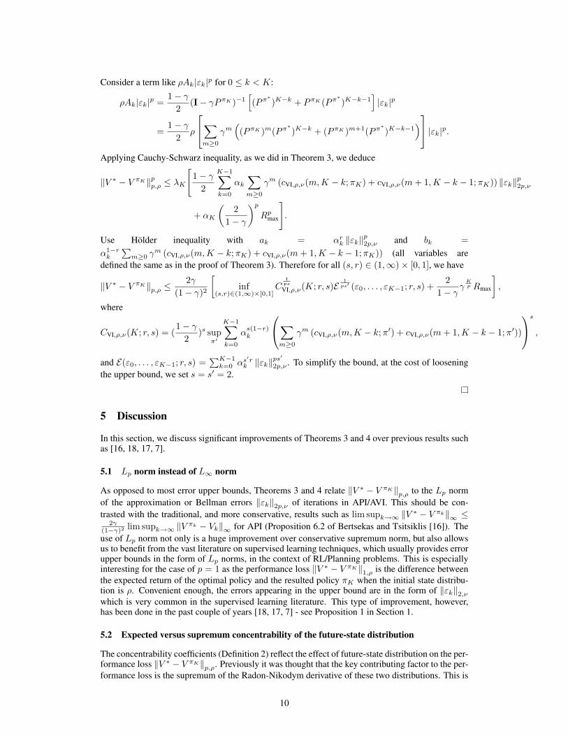
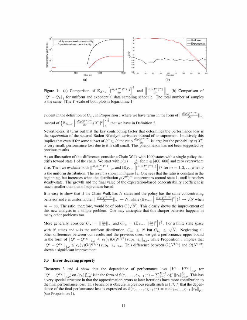
Figure 1: (a) Comparison of EX∼ν

[

|d(ρ(P π)m)dν |2

]12

and

∥

∥

∥

d(ρ(P π)m)dν

∥

∥

∥

∞(b) Comparison of

‖Q∗ − Qk‖1 for uniform and exponential data sampling schedule. The total number of samplesis the same. [The Y -scale of both plots is logarithmic.]

evident in the definition of Cρ,ν in Proposition 1 where we have terms in the form of ||d(ρ(P π)m)dν ||∞

instead of(

EX∼ν

[

|d(ρ(P π)m)dν (X)|2

])12

that we have in Definition 2.

Nevertheless, it turns out that the key contributing factor that determines the performance loss isthe expectation of the squared Radon-Nikodym derivative instead of its supremum. Intuitively this

implies that even if for some subset of X ′ ⊂ X the ratiod(ρ(P π)m)

dν is large but the probability ν(X ′)is very small, performance loss due to it is still small. This phenomenon has not been suggested byprevious results.

As an illustration of this difference, consider a Chain Walk with 1000 states with a single policy thatdrifts toward state 1 of the chain. We start with ρ(x) = 1

201 for x ∈ [400, 600] and zero everywhere

else. Then we evaluate both ||d(ρ(P π)m)dν ||∞ and (EX∼ν

[

|d(ρ(P π)m)dν |2

]

)12 for m = 1, 2, . . . when ν

is the uniform distribution. The result is shown in Figure 1a. One sees that the ratio is constant in thebeginning, but increases when the distribution ρ(Pπ)m concentrates around state 1, until it reachessteady-state. The growth and the final value of the expectation-based concentrability coefficient ismuch smaller than that of supremum-based.

It is easy to show that if the Chain Walk has N states and the policy has the same concentrating

behavior and ν is uniform, then ||d(ρ(P π)m)dν ||∞ → N , while (EX∼ν

[

|d(ρ(P π)m)dν |2

]

)12 →

√N when

m → ∞. The ratio, therefore, would be of order Θ(√

N). This clearly shows the improvement ofthis new analysis in a simple problem. One may anticipate that this sharper behavior happens inmany other problems too.

More generally, consider C∞ = ||dµdν ||∞ and CL2

= (EX∼ν

[

|dµdν |2

]

)12 . For a finite state space

with N states and ν is the uniform distribution, C∞ ≤ N but CL2≤

√N . Neglecting all

other differences between our results and the previous ones, we get a performance upper bound

in the form of ‖Q∗ − QπK‖1,ρ ≤ c1(γ)O(N1/4) supk ‖εk‖2,ν , while Proposition 1 implies that

‖Q∗ − QπK‖1,ρ ≤ c2(γ)O(N1/2) supk ||ǫk||2,ν . This difference between O(N1/4) and O(N1/2)shows a significant improvement.

5.3 Error decaying property

Theorems 3 and 4 show that the dependence of performance loss ‖V ∗ − V πK‖p,ρ (or

‖Q∗ − QπK‖p,ρ) on {εk}K−1k=0 is in the form of E(ε0, . . . , εK−1; r) =

∑K−1k=0 α2r

k ‖εk‖2p2p,ν . This has

a very special structure in that the approximation errors at later iterations have more contribution tothe final performance loss. This behavior is obscure in previous results such as [17, 7] that the depen-dence of the final performance loss is expressed as E(ε0, . . . , εK−1; r) = maxk=0,...,K−1 ‖εk‖p,ν

(see Proposition 1).

11

This property has practical and algorithmic implications too. It says that it is better to put moreeffort on having a lower Bellman or approximation error at later iterations of API/AVI. This, forinstance, can be done by gradually increasing the number of samples throughout iterations, or to usemore powerful, and possibly computationally more expensive, function approximators for the lateriterations of API/AVI.

To illustrate this property, we compare two different sampling schedules on a simple MDP. TheMDP is a 100-state, 2-action chain similar to Chain Walk problem in the work of Lagoudakis andParr [5]. We use AVI with a lookup-table function representation. In the first sampling schedule,every 20 iterations we generate a fixed number of fresh samples by following a uniformly randomwalk on the chain (this means that we throw away old samples). This is the fixed strategy. In theexponential strategy, we again generate new samples every 20 iterations but the number of samplesat the kth iteration is ckγ . The constant c is tuned such that the total number of both samplingstrategy is almost the same (we give a slight margin of about 0.1% of samples in favor of the fixedstrategy). What we compare is ‖Q∗ − Qk‖1,ν when ν is the uniform distribution. The result can be

seen in Figure 1b. The improvement of the exponential sampling schedule is evident. Of course, onemay think of more sophisticated sampling schedules but this simple illustration should be sufficientto attract the attention of practitioners to this phenomenon.

5.4 Restricted search over policy space

One interesting feature of our results is that it puts more structure and restriction on the way policiesmay be selected. Comparing CPI,ρ,ν(K; r) (Theorem 3) and CVI,ρ,ν(K; r) (Theorem 4) with Cρ,ν

(Proposition 1) we see that:

(1) Each concentrability coefficient in the definition of CPI,ρ,ν(K; r) depends only on a single ortwo policies (e.g., π′

k in cPI1,ρ,ν(K − k,m;π′k)). The same is true for CVI,ρ,ν(K; r). In contrast, the

mth term in Cρ,ν has π1, . . . , πm as degrees of freedom, and this number is growing as m → ∞.

(2) The operator sup in CPI,ρ,ν and CVI,ρ,ν appears outside the summation. Because of that, weonly have K + 1 degrees of freedom π′

0, . . . , π′K to choose from in API and remarkably only a

single degree of freedom in AVI. On the other other hand, sup appears inside the summation in thedefinition of Cρ,ν . One may construct an MDP that this difference in the ordering of sup leads to anarbitrarily large ratio of two different ways of defining the concentrability coefficients.

(3) In API, the definitions of concentrability coefficients cPI1,ρ,ν , cPI2,ρ,ν , and cPI3,ρ,ν (Defini-tion 2) imply that if ρ = ρ∗, the stationary distribution induced by an optimal policy π∗, then

cPI1,ρ,ν(m1, m2;π) = cPI1,ρ,ν(·, m2;π) = (EX∼ν

[

∣

∣

∣

d(ρ∗(P π)m2 )dν

∣

∣

∣

2]

)12 (similar for the other two

coefficients). This special structure is hidden in the definition of Cρ,ν in Proposition 1, and insteadwe have an extra m1 degrees of flexibility.

Remark 1. For general MDPs, the computation of concentrability coefficients in Definition 2 isdifficult, as it is for similar coefficients defined in [18, 17, 7].

6 Conclusion

To analyze an API/AVI algorithm and to study its statistical properties such as consistency or con-vergence rate, we require to (1) analyze the statistical properties of the algorithm running at eachiteration, and (2) study the way the policy approximation/Bellman errors propagate and influencethe quality of the resulted policy.

The analysis in the first step heavily uses tools from the Statistical Learning Theory (SLT) literature,e.g., Gyorfi et al. [22]. In some cases, such as AVI, the problem can be cast as a standard regressionwith the twist that extra care should be taken to the temporal dependency of data in RL scenario.The situation is a bit more complicated for API methods that directly aim for the fixed-point solution(such as LSTD and its variants), but still the same kind of tools from SLT can be used too – see Antoset al. [7], Maillard et al. [8].

The analysis for the second step is what this work has been about. In our Theorems 3 and 4, wehave provided upper bounds that relate the errors at each iteration of API/AVI to the performance

12

loss of the whole procedure. These bounds are qualitatively tighter than the previous results such asthose reported by [18, 17, 7], and provide a better understanding of what factors contribute to thedifficulty of the problem. In Section 5, we discussed the significance of these new results and theway they improve previous ones.

Finally, we should note that there are still some unaddressed issues. Perhaps the most important oneis to study the behavior of concentrability coefficients cPI1,ρ,ν(m1, m2;π), cPI2,ρ,ν(m1, m2;π1, π2),and cVI,ρ,ν(m1, m2;π) as a function of m1, m2, and of course the transition kernel P of MDP. Abetter understanding of this question alongside a good understanding of the way each term εk inE(ε0, . . . , εK−1; r) behaves, help us gain more insight about the error convergence behavior of theRL/Planning algorithms.

References

[1] Damien Ernst, Pierre Geurts, and Louis Wehenkel. Tree-based batch mode reinforcementlearning. Journal of Machine Learning Research, 6:503–556, 2005.

[2] Martin Riedmiller. Neural fitted Q iteration – first experiences with a data efficient neuralreinforcement learning method. In 16th European Conference on Machine Learning, pages317–328, 2005.

[3] Amir-massoud Farahmand, Mohammad Ghavamzadeh, Csaba Szepesvari, and Shie Mannor.Regularized fitted Q-iteration for planning in continuous-space markovian decision problems.In Proceedings of American Control Conference (ACC), pages 725–730, June 2009.

[4] Remi Munos and Csaba Szepesvari. Finite-time bounds for fitted value iteration. Journal ofMachine Learning Research, 9:815–857, 2008.

[5] Michail G. Lagoudakis and Ronald Parr. Least-squares policy iteration. Journal of MachineLearning Research, 4:1107–1149, 2003.

[6] Steven J. Bradtke and Andrew G. Barto. Linear least-squares algorithms for temporal differ-ence learning. Machine Learning, 22:33–57, 1996.

[7] Andras Antos, Csaba Szepesvari, and Remi Munos. Learning near-optimal policies withBellman-residual minimization based fitted policy iteration and a single sample path. MachineLearning, 71:89–129, 2008.

[8] Odalric Maillard, Remi Munos, Alessandro Lazaric, and Mohammad Ghavamzadeh. Finite-sample analysis of bellman residual minimization. In Proceedings of the Second Asian Con-ference on Machine Learning (ACML), 2010.

[9] Amir-massoud Farahmand, Mohammad Ghavamzadeh, Csaba Szepesvari, and Shie Mannor.Regularized policy iteration. In D. Koller, D. Schuurmans, Y. Bengio, and L. Bottou, editors,Advances in Neural Information Processing Systems 21, pages 441–448. MIT Press, 2009.

[10] J. Zico Kolter and Andrew Y. Ng. Regularization and feature selection in least-squares tempo-ral difference learning. In ICML ’09: Proceedings of the 26th Annual International Conferenceon Machine Learning, pages 521–528, New York, NY, USA, 2009. ACM.

[11] Xin Xu, Dewen Hu, and Xicheng Lu. Kernel-based least squares policy iteration for reinforce-ment learning. IEEE Trans. on Neural Networks, 18:973–992, 2007.

[12] Tobias Jung and Daniel Polani. Least squares SVM for least squares TD learning. In In Proc.17th European Conference on Artificial Intelligence, pages 499–503, 2006.

[13] Gavin Taylor and Ronald Parr. Kernelized value function approximation for reinforcementlearning. In ICML ’09: Proceedings of the 26th Annual International Conference on MachineLearning, pages 1017–1024, New York, NY, USA, 2009. ACM.

[14] Sridhar Mahadevan and Mauro Maggioni. Proto-value functions: A Laplacian frameworkfor learning representation and control in markov decision processes. Journal of MachineLearning Research, 8:2169–2231, 2007.

[15] Alborz Geramifard, Michael Bowling, Michael Zinkevich, and Richard S. Sutton. iLSTD: El-igibility traces and convergence analysis. In B. Scholkopf, J. Platt, and T. Hoffman, editors,Advances in Neural Information Processing Systems 19, pages 441–448. MIT Press, Cam-bridge, MA, 2007.

13

[16] Dimitri P. Bertsekas and John N. Tsitsiklis. Neuro-Dynamic Programming (Optimization andNeural Computation Series, 3). Athena Scientific, 1996.

[17] Remi Munos. Performance bounds in lp norm for approximate value iteration. SIAM Journalon Control and Optimization, 2007.

[18] Remi Munos. Error bounds for approximate policy iteration. In ICML 2003: Proceedings ofthe 20th Annual International Conference on Machine Learning, 2003.

[19] Dimitri P. Bertsekas and Steven E. Shreve. Stochastic Optimal Control: The Discrete-TimeCase. Academic Press, 1978.

[20] Richard S. Sutton and Andrew G. Barto. Reinforcement Learning: An Introduction (AdaptiveComputation and Machine Learning). The MIT Press, 1998.

[21] Csaba Szepesvari. Algorithms for Reinforcement Learning. Morgan Claypool Publishers,2010.

[22] Laszlo Gyorfi, Michael Kohler, Adam Krzyzak, and Harro Walk. A Distribution-Free Theoryof Nonparametric Regression. Springer Verlag, New York, 2002.

14