Error Detection and Control for Nonlinear Shell Analysis · ERROR DETECTION AND CONTROL FOR...
14
NASA Technical Memorandum 102723 Error Detection and Control for Nonlinear Shell Analysis Sussn L, McClesry Lockheed Engineering and Sciences Compsay Hsmpton, Virginis Normsa F. Knight, Jr, NASA Lsngley Eemesrch Center Hsmptonm Virglnis (NASA-TM-102?2.3) FRR,r')R DETECTION AND CONT_qL FOR N_NLINEAR ._HELL ANALY'_IS (NASA) 12 p CSCL 20K August 1990 _3/39 N90-28371 N/LqA Nal_onal A,eran_tut_[;t_ ilncJ Space Adm!npF, irill_an LJngley Iquuroh Cenler Hampton, Virginia23885-5225 https://ntrs.nasa.gov/search.jsp?R=19900019561 2018-07-14T01:19:02+00:00Z
-
Upload
phungduong -
Category
Documents
-
view
244 -
download
0
Transcript of Error Detection and Control for Nonlinear Shell Analysis · ERROR DETECTION AND CONTROL FOR...

NASA Technical Memorandum 102723
Error Detection and Control for
Nonlinear Shell Analysis
Sussn L, McClesryLockheed Engineering and Sciences Compsay
Hsmpton, Virginis
Normsa F. Knight, Jr,
NASA Lsngley Eemesrch Center
Hsmptonm Virglnis
(NASA-TM-102?2.3) FRR,r')R DETECTION AND
CONT_qL FOR N_NLINEAR ._HELL ANALY'_IS (NASA)
12 p CSCL 20K
August 1990
_3/39
N90-28371
N/LqANal_onal A,eran_tut_[;t_ilncJSpace Adm!npF,irill_an
LJngley Iquuroh CenlerHampton,Virginia23885-5225
https://ntrs.nasa.gov/search.jsp?R=19900019561 2018-07-14T01:19:02+00:00Z


ERROR DETECTION AND CONTROL FOR NONLINEAR SHELL ANALYSIS
Susan L. McCleary
Lockheed Engineering and Sciences Company
Norman F. Knight, Jr.
NASA Langley Research Center
MS 244, NASA Langley Research Center, Hampton, VA 23665-5225 USA
SUMMARY
A problem-adaptive solution procedure for improving the re,ability of finite element
solutions to geometrically nonlinear shell-type problems Is presented. The strategy
Incorporates automatic error detection and control and Includes an iterative procedure
which utilizes the solution at one load step from one finite element model to obtain
an equivalent solution at the same load step on a more refined model. Representative
nonlinear shell problems are solved.
INTRODUCTION
Much of the research In adaptive finite element structural analysis has centered on the development
of techniques for use in linear analysis. However, the need for an adaptive strategy Is even more
important In nonlinear analysis where a given finite element model may perform adequately for a
certain range of loading (e.g., for the first several load steps) and become grossly Inadequate for
another range of loading (e.g., for the last several load steps). Recent work at the NASA Langley
Research Center has focused on the development of an adaptive nonlinear analysis procedure for
shell structures (McCleary {1]). This adaptive analysis procedure integrates three primary compo-
nents Into the nonlinear solution procedure: an automatic error detection strategy, an automatic
error control strategy, and a reference state definition technique. Each of these components are
described herein, and the use of the procedure is demonstrated on two geometrically nonlinear shell
problems.
THE ADAPTIVE ANALYSIS PROCEOURE
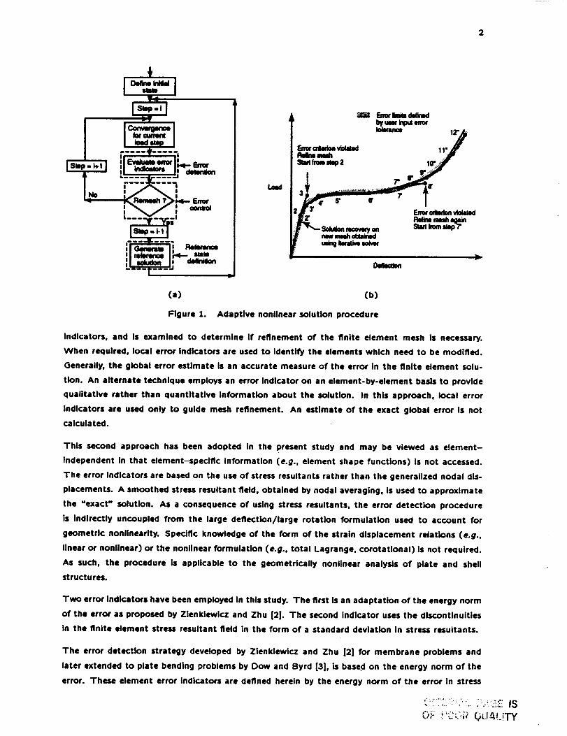
The primary components of the adaptive non,near solution procedure are identified In the algorithm
flowchart of Figure l(a). The use of this algorithm to predict a nonlinear response curve is
Illustrated In Figure l(b). The analyst defines an error tolerance which sets boundaries on the
deviation of the calculated response from the converged response. At some load step, the initial
finite element discretizatlon may predict a response which violates the prescribed error tolerance
(e.g., see step 3 In Figure 1). At this point, a new finite element model is generated and the
solution procedure backs up to the previous load step (see steps 2 and 2_ In the figure). Once an
equivalent solution has been obtained at the previous load step for the new finite element mesh,
the adaptive procedure proceeds until the response again violates the prescribed error tolerance
(e.g., step 8' on the figure).
Many adaptive mesh refinement strategies employ a two tiered a posteriorl error detection tech-
nique. In this technique, a global error estimate is computed as the summation of the local error
2
(a) (b)
Figure 1. Adaptive nonlinear solution procedure
indicators, and Is examined to determine If refinement of the finite element mesh Is necessary.
When required, local error indicators are used to Identify the elements which need to be modified.
Generally, the global error estimate Is an accurate measure of the error In the finite element solu-
tion. An alternate technique employs an error Indicator on an element-by-element basis to provide
qualitative rather than quantitative Information about the solution. In this approach, local error
Indicators are used only to guide mesh refinement. An estimate of the exact global error Is not
calculated.
This second approach has been adopted In the present study and may be viewed as element-
independent In that element-specific information (e.g., element shape functions) is not accessed.
The error Indicators are based on the use of stress resultants rather than the generalized nodal dis-
placements. A smoothed stress resultant field, obtained by nodal averaging, is used to approximate
the "exact" solution. As a consequence of using stress resultants, the error detection procedure
is Indirectly uncoupled from the large deflection/large rotation formulation used to account for
geometric nonlinearity. Specific knowledge of the form of the strain displacement relations (e.g.,
linear or nonlinear) or the nonlinear formulation (e.g., total Lagrange, corotational) Is not required.
As such, the procedure is applicable to the geometrically nonlinear analysis of plate and shell
structures.
Two error Indicators have been employed in this study. The first Is an adaptation of the energy norm
of the error as proposed by Zlenklewlcz and Zhu [2|. The second Indicator uses the discontlnuiUes
in the finite element stress resultant field in the form of a standard deviation In stress resultants.
The error detection strategy developed by Zienklewicz and Zhu [2] for membrane problems and
later extended to plate bending problems by Dow and Byrd [3], is based on the energy norm of the
error. These element error indicators are defined herein by the energy norm of the error In stress
OF PC_O[,_ Q_.JA!,.!TY
3
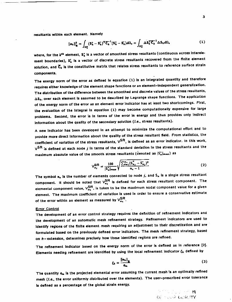
resultants within each element. Namely
I1.,11_
where, for the k sh element, S_, is a vector of smoothed stress resultants (continuous across Interele-
ment boundaries), S; Is a vector of discrete stress resultants recovered from the finite element
solution, and _r Is the constitutive matrix that relates stress resultants to reference surface strain
components.
The energy norm of the error as defined In equation (1) is an Integrated quantity and therefore
requires either knowledge of the element shape functions or an element-independent generalization.
The distribution of the dl/l'erence between the smoothed and discrete values of the stress resultants,
ASk, over each element Is assumed to be described by Lagrange shape functions. The application
of the energy norm of the error as an element error Indicator has at least two shortcomings. First,
the evaluation of the Integral in equation (1) may become computationally expensive for large
problems. Second, the error is in terms of the error in energy and thus provides only Indirect
Information about the quality of the secondary solution (Le., stress resultants).
A new Indicator has been developed In an attempt to minimize the computational effort and to
provide more direct Information about the quality of the stress resultant field. From statistics, the
coefficient of variation of the stress resultants, V SR, Is defined as an error Indicator. In this work,
V SR is defined at each node j In terms of the standard deviation In the stress resultants and the
maximum absolute value of the smooth stress resultants ((lenoted as JS_I,...) as
100 /I:_',(s:_ - s:_)' (2)= V -.-'
The symbol _, is the number of elements connected to node j, and S. is a single stress resultant
component. It should be noted that V_.R is defined for each stress resultant component. The
elemental component value, VaSR, Is taken to be the maximum nodal component value for a given
element. The maximum coefficient of variation is used in order to ensure a conservative estimate
of the error within an element as measured by V.5R.
I_rror Control
The development of an error control strategy requires the definition of refinement Indicators and
the development of an automatic mesh refinement strategy. Refinement Indicators are used to
Identify regions of the finite element mesh requiring an adjustment to their dlscretizatlon and are
formulated based on the previously defined error indicators. The mesh refinement strategy, based
on /I-extension, determines precisely how these identified regions are refined.
The refinement Indicator based on the energy norm of the error Is defined as in reference [2].
Elements needing refinement are Identified by using the local refinement indicator _ defined by
_h= _ (3)e.
The quantity em is the projected elemental error assuming the current mesh Is an optimally refined
mesh (Le., the error uniformly distributed over the elements). The user-prescribed error tolerance
is defined as a percentage of the global strain energy.
: • .... FS
4
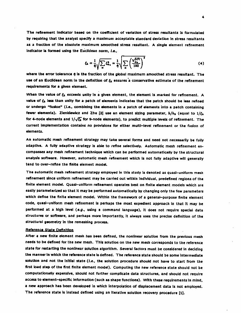
The refinement indicator based on the coeffident of variation of stress resultants is formulated
by requiring that the analyst specify a maximum acceptable standard deviation In stress resultants
as a fraction of the absolute maximum smoothed stress resultant. A single element refinement
Indicator is formed using the Euclidean norm, Le.,
(4)
where the error tolerance _ is the fraction of the global maximum smoothed stress resultant. The
use of an Euclidean norm In the definition of _ ensures "a conservative estimate of the refinement
requirements for a given element.
When the value of _ exceeds unity In a given element, the element Is marked for refinement. A
value of _ less than unity for a patch of elements Indicates that the patch should be less refined
or undergo "fusion" (i.e., combining the elements in a patch of elements into a patch containing
fewer elements). Zlenklewicz and Zhu [2] use an element sizing parameter, h/hh (equal to 1/_b
for ,I-node elements and 1/_" for 9-node elements), to predict multiple levels of refinement. The
current Implementation contains no provisions for either multi--level refinement or the fusion of
elements.
An automatic mesh refinement strategy may take several forms and need not necessarily be fully
adaptive. A fully adaptive strategy Is able to refine selectively. Automatic mesh refinement en-
compasses any mesh refinement technique which can be performed automatically by the structural
analysis software. However, automatic mesh refinement which Is not fully adaptive will generally
tend to over-refine the finite element model.
The automatic mesh refinement strategy employed in this study is denoted as quasi-uniform mesh
refinement since uniform refinement may be carried out within Individual, predefined regions of the
finite element model. Quasi-uniform refinement operates best on finite element models which are
easily parameterized so that it may be performed automatically by changing only the few parameters
which define the finite element model. Withtn the framework of a general-purpose finite element
code, quasi-uniform mesh refinement Is perhaps the most expedient approach in that It may be
performed at a high level (e.g., using a command language), It does not require special data
structures or software, and perhaps more Importantly, it always uses the precise definition of the
structural geometry In the remeshlng process.
Reference State Definition
After a new finite element mesh has been defined, the nonlinear solution from the previous mesh
needs to be defined for the new mesh. This solution on the new mesh corresponds to the reference
state for restarting the nonlinear solution algorithm. Several factors must be considered In deciding
the manner in which the reference state is defined. The reference state should be some Intermediate
solution and not the initial state (I.e., the solution procedure should not have to start from the
first toad step of the first finite element model). Computing the new reference state should not be
computationally expensive, should not further complicate data structures, and should not require
access to element-specific information (such as shape functions). With these requirements in mind,
a new approach has been developed In which Interpolation of displacement data Is not employed.
The reference state is Instead defined using an iterative solution recovery procedure [1].

form applied displacement vector.j=l
do for J < max_d/ters
<_, = <;;form tangent stifiness matrix based on _-1
solve KI_ l _-l = f_-t using PCG methodcalculate error:• = tt - <:: tt/, <-, tt
Ire < td exiti=i+1
enddo
Figure 2. Iteratlve solution recovery.
The strategy for determining a consistent solution for a refined mesh Is summarized In Figure 2.
This strategy uses the nonlinear solution at the previous load step (step i - 1) from the previous
finite element model, to generate an applied displacement vector for the solution at the same load
step on the new finite element model. Only those nodes which are new to the finite element model
are left unconstrained during the iteration cycle. An initial estimate of the solution vector is formed
by initializing the displacements at the new nodes to zero. While these initial displacements may
be assigned values other than zero, doing so has not proven to alter significantly the convergence
characteristics of the iterative solution recovery procedure. Once formed, the Initial estimate is used
to generate a tangent stlfiness matrix and serves as an Initial guess for a preconditioned conjugate
gradient (PCG) Iteratlve solver. The solution _-1 Is compared to the solution at iteration j - 1
(Le., _-_) and the solution recovery error Is measured by
_ au__z_,_-_ (s)¢_u" "T " '"
where Z_u__l = _-l -_--'_- If the error, e/. is less than the specified error tolerance, a converged
solution at step i- 1 has been achieved. If the error Is greater than the Specified tolerance, a new
tangent stlfiness matrix is formed based on the i t_ displacement solution. The procedure continues
until a converged solution for load step i- 1 on the new finite element mesh is obtained. The
algorithm then proceeds to load step i and obtains an Improved solution at load step d 'on the new
finite element mesh.
This technique Is particularly effective, and only efficient, when an ]terative equation solver (e.g.,
PCG technique) is used. In this case, the solution __-_ is used as an Initial solution for the ]teratlve
solver at Iteration j (I.e., as an Initial guess for _-z), thereby Increasing the rate of convergence for
the solver. While direct solvers may be used, they require a complete factorizatlon of the tangent
stiffness matrix at each Iteration and will take roughly the same amount of time for each solution
iteration. An Iterative solver will generally require an ever decreasing number of Internal iterations
as the overall solution recovery process converges.
NUMERICAL RESULTS
The adaptive procedure described herein has been developed using the framework of the CSM
Testbed [4]. Control of the analysis procedure Is implemented using the command language

5
1800 _R
Load,_,i_ I""" r- .,_ • Mo_2
I l • Mo_3mL ..,_c • Modi4"--I- .._ • Models
I ..,+r --trill
0 E ,,, 1_Tpsl R .. 1.0 Inch.010 .o3o o4o +.o.+ L'WA I'
Norn_ dellectlon, In.
Flgure 3. Peer-shaped cyllnder: geometry, propertles, and response.
capablllty of the CSM Testbed. Moreover, a stand-alone Fortran processor has been developed for
evaluating the varlous error and refinement Indlcators. A total Lagranglan formulation Is used for
the nonllnear problem descrlptlon, and the solution strategy Incorporates the Rlks/Crlsfield arc-
length approach wlthln a modified Newton-Raphson procedure to solve the system of nonllnear
algebralc equatlons (see [I] for detalls). The refinement Indicator, G, dlsplayed in the following
sectlons Is analogous to the element sizing-parameter prevlously dlscussed and Is defined as (i = I/+i
for 4-node elements and as <_i= i/vr_ " for 9-node elements.
In subsequent sectlon/, the results of two nonllnear shell analyses are presented. Both problems
Involve structures which exhibit complex nonllnear behavior. The first problem, the collapse of a
pear-shaped cyllnder, demonstrates the use of the adaptive procedure on an Isotroplc, geometrically
regular (rectangular elements are used throughout the domain) problem. Correlation wlth prevlously
published results Is shown. The second problem, the buckllng of a cyllndrlcal panel wlth a hole,
demonstrates the use of the adaptlve procedure on a composite, geometrically Irregular (skewed
elements are requlred to model the central circular hole) problem. Correlations wlth test data and
prevlously publLshed analytlcal results are shown.
Pear-Shaoed Cvllnder
The pear-shaped cylinder shown In Figure 3 has been adopted by many researchers and the be-
havlor of thli cyllnder subject to a uniform end-shortenlng Investlgated (see Hartung and Ball
IS]). The cyllnder response becomes nonllnear at low values of applied end-shortening, and the
normal defiectlons of the fiat portlons of the cyllnder Increase rapidly with Increases In loadlng.
The symmetry exhibited by the structure allows the analysis to be performed on one fourth of the
cyllnder.
Quasl-unlform mesh refinement has been used for error control. The finite element mesh has been
dlvlded Into four groups of elements. Element group I contalns the elements In the 45* arc at
the top of the cylinder, element group 2 contains the elements In the fiat segment between the
two curved segments, element group 3 contalns the elements In the 135 ° arc, and element group
4 contains the elements In the bottom fiat segment of the cylinder. Clrcumferentlal refinement

7
A CB
D E
5
6,
8
9
10
Figure 4. Refinement indicators, _k, for finite element models 1 through 5.Models A-E correspond to points A-E on Figure 3.
within any individual group of elements was unrestricted. Whenever all four element groups required
refinement simultaneously, refinement through the depth of the cylinder was carried out in a uniform
fashion (Le., for all elements in all groups). Command language procedures were used to direct
the mesh refinement based on the original cylinder geometry.
The nonlinear response of a series of five finite element models Is also shown In Figure 3. As
shown In the figure, once the solution starts to deviate from the converged solution (603 nodes,
132 g-node Assumed Natural-coordinate Strain (9ANS) elements [6]), mesh refinement occurs.
The iterative solution recovery algorithm then defines the reference state for the restart of the
nonlinear solution procedure. The collapse load is 2471 Ibs., within 5% of the collapse load reported
by Hartung and Ball {5].
For this series of models, refinement is based on the energy norm of the error with a 10% error
tolerance; each model Is composed of 9ANS elements. The refinement indicators _ for the set of
finite element models are shown In Figure 4. Initially, refinement was required only within the fiat
portions of the finite element model where significant nonlinear behavior was present. At higher
values of load, the curved segments of the cylinder also needed refinement since these segments
began to exhibit large normal deflections. Similar results are obtained using the coefficient of
variation of stress resultants with an error tolerance of 10%.
COmDosite Cylindrical Panel
The postbuckllng response of axially compressed composite cylindrical panels with holes has been
a subject of research for several years (e.g., Knight and Starnes [7]). This problem is characterized
by large local deformations In the neighborhood of the hole which cause ply delaminations to occur
In the postbuckling range. The panel analyzed herein is loaded with a uniform end-shortening
8
.0020 *
oo_ol-- ,J[- • M_ 2• i IDA / * .__J*.!3
l • Mo l4
J
T300_208 gr_oC_e-epoxy _o.
16-ply quui-lsotropic laminate15-inch ridlus
14-1ndl square pladorm2-inch circular cutout
0 .0010 .0020 .0030
Normdzed ,nd-_enieg
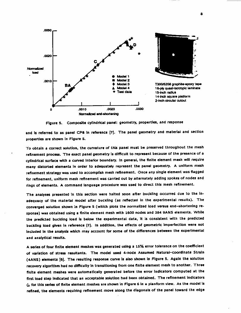
Figure 5. Composite cylindrical panel: geometry, properties, and response
and is referred to as panel CP8 In reference [7]. The panel geometry and material and section
properties are shown in Figure 5.
To obtain a correct solution, the curvature of this panel must be preserved throughout the mesh
refinement process. The exact panel geometry is difficult to represent because of the presence of a
cylindrical surface with a curved Interior boundary. In general, the finite element mesh will require
many distorted elements In order to adequately represent the panel geometry. A uniform mesh
refinement strategy was used to accomplish mesh refinement. Once any single element was flagged
for refinement, uniform mesh refinement was carried out by alternately adding spokes of nodes and
rings of elements. A command language procedure was used to direct this mesh refinement.
The analyses presented In this section were halted soon after buckling occurred due to the in-
adequacy of the material model after buckling (as reflected In the experimental results). The
converged solution shown In Figure 5 (which plots the normalized load versus end-shortening re-
sponse) was obtained using a finite element mesh with 1600 nodes and 384 9ANS elements. While
the predicted buckling load is below the experimental data, it is consistent with the predicted
buckling load given in reference [7]. In addition, the effects of geometric Imperfection were not
included in the analysLs which may account for some of the differences between the experimental
and analytical results.
A series of four finite element meshes was generated using a 15% error tolerance on the coefficient
of variation of stress resultants. The model used 4-node Assumed Natural-coordinate 5train
(4ANS) elements [6]. The resulting response curve Is also shown in Figure 5. Again the solution
recovery algorithm had no difilculty in transitionlng from one finite element mesh to another. Three
finite element meshes were automatically generated before the error Indicators computed at the
first load step Indicated that an acceptable solution had been obtained. The refinement Indicators
for this series of finite element meshes are shown In Figure 6 in a planform view. As the model Is
refined, the elements requiring refinement move along the diagonals of the panel toward the edge

9
A B
0
1
2
3
4
5
6
7
8
9
C D 10Figure 6. Refinement Indicators, (k, for finite element models 1 through 4.
Models A-D correspond to points A-O on Figure 5.
of the hole where large gradients occur.
(;9m0utatlonal Effort
One of the goals of the work described thus far Is to show that the adaptive nonlinear solution
strategy presented herein can be efficient. Satisfying this goal requires that the computational
time required for performing a nonlinear analysis using the adaptive procedure as outlined should
not substantially exceed the computational time required for a nonlinear analysis performed using
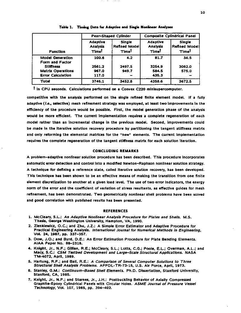
a single refined finite element model. Timing data for both the pear-shaped cylinder and the
composite cylindrical panel are summarized in Table 1. For each case, the single refined finite
element model was selected to be the final finite element model generated by the adaptive solution
procedure. This single refined model was defined only after the adaptive analysis was performed.
In general, multiple models and analyses would have been required to obtain a reliable solution.
In the case of the pear-shaped cylinder, the analysis performed using the adaptive procedure
required only approximately 9% more CPU time than the analysis performed using the single refined
finite element model. In the case of the composite cylindrical panel, the analysis performed using
the adaptive procedure required approximately 19% more CPU time than the analysis performed
using a single refined model. This difference In the additional percentage of CPU time required is
attributable to the fact that all of the mesh refinement occurs within the first two load steps of
the analysis of the composite panel. While the analysis performed using the single refined model
required less CPU time for both problems, the reliability of the solutions can only be assessed
by a complete re-solution on a different mesh. In both cases, the total CPU time required for
computing two complete nonlinear solutions would be greater than the CPU tlme required to
perform the single adaptive analysis.
The results shown In the table are very encouraging in that the adaptive analysis Is at least
10
Table 1. T1mlnE Date foe Adaptive and Sinsle Nonlinear Analyses
Function
Model Generation
Form and Factor
Stlflrness
Matrix OperationsError Calculation
Pear-Shaped Cylinder
Adaptive
Analysis
Tlmet
100.6
2561.2
967.0
117.0
SingleRefined Model
Tlmet
4.2
2497.5
949.71
Composite Cylindrical Panel
Adaptive
Analysis
Tlmet
81.7
3254.9
$84.S
435.3
SingleRefined Model
Timer
34.5
3062.0
575.0
Total 3746.1 3452.8 4358.6 3672.5
t In CPU seconds. Calculations performed on a Convex C220 minisupercomputer.
competitive with the analysis performed on the single refined finite element model. If a fully
adaptive (i.e., selective) mesh refinement strategy was employed, at least two Improvements In the
effidency of the procedure would be possible. First, the model generation phase of the analysis
would be more efficient. The current Implementation requires a complete regeneration of each
model rather than an Incremental change in the previous model. Second, improvements could
be made in the Iterative solution recovery procedure by partitioning the tangent stiffness matrix
and only reforming the elemental matrices for the "new" elements. The current Implementation
requires the complete regeneration of the tangent stiffness matrix for each solution iteration.
CONCLUDING REMARKS
A problem-adaptive nonlinear solution procedure has been described. This procedure Incorporates
automatic error detection and control Into a modified Newton-Raphson nonlinear solution strategy.
A technique for defining a reference state, called iterative solution recovery, has been developed.
This technique has been shown to be an effective means of making the transition from one finite
element discretlzation to another at a given load level. The use of two error indicators, the energy
norm of the error and the coefficient of variation of stress resultants, as effective guides for mesh
refinement, has been demonstrated. Two geometrically nonlinear shell problems have been solved
and good correlation with published results has been presented.
REFERENCES
1. McCleary, S.l..: An Adaptive Nonlinear Analysis Procedure for Plates and Shells. M.S.Thesis, George Washington UnlversJty, Hampton, VA, 1990.
2. Zlenklewicz, D.C.; and Zhu, J.Z.: A Simple Error Estimator and Adaptive Procedure for
Practical Engineering Analysis. International Journal for Numerical Methods in Engineering,VoL 24, 1987, pp. 337-3S7.
3. Dow, J.O.; and Byrd, D.E.: An Error Estimation Procedure for Plate Bending Elements.AIAA Paper No. 88-2318.
4. Knight, Jr., N.F.; GIIIlan, R.E., McCleary, S.L.; Lotts, C.G.; Poole, E.L.; Overman, A.L.; andMacy, S.C.: CSM Testbed Development and Large-Scale Structural Applications. NASATM-4072, April, 1989.
S. Hartung, R.F.; and Ball, R.E.: A Comparison of Several Computer Solutions to ThreeStructural Shell Analysis Problems. AFFDL-TR-73-15, U.S. Air Force, April, 1973.
6. Stanley, G.M.: Continuum-Based Shell Elements. Ph.D. Dissertation, Stanford University,Stanford, CA, 1985.
7. Knight, Jr., N.F.; and Starnes, Jr., J.H.: Postbuckling Behavior of Axially Compressed
Graphite-Epoxy Cylindrical Panels with Circular Holes. ASME Journal of Pressure VesselTechnology, VOl. 107, 198S, pp. 394-402.

NallOn al Aefonaullcs and
Space Ad m,rl_Sll _ltOn
I. NASARep°rtTM-102723N°' I 2. Government Accession No.
4. Title _rLd Subtitle
Error Detection and Control for Nonlinear Shell Analysis
7. Author(s)
Susan L. McCleary
Norman F. Knight, Jr.
9. Performing Organisation Nsrae and Address
NASA Langley Research Center
Hampton, VA 23665-5225
12. Sponsoring Agency Name and Address
National Aeronautics and Space Administration
Washington, DC 20546-0001
Report Documentation Page
3. Reclpient's Catalog No.
8. Report Date
August 1990
6. Performing Organisation Code
8. Performing Organisation Report No.
10. Work Unit No.
505-63-01-10
11. Contract or Gr_nt No.
13. Type of Report and Period Covered
Technical Memorandum
14. Sponsoring Agency Code
15. Supplementary Notes
Susan L. McCleary, Lockheed Engineering and Sciences Company, Hampton, Virginia
Norman F. Knight, Jr., Formerly NASA Langley Research Center, Hampton, Virginia 23665
Currently Clemson University, Clemson, South Carolina
Presented at the Sixth World Congress on Finite Element Methods, October 1-5, 1990, Banff', Alberta,
Canada
16. Abstract
A problem-adaptive solution procedure for improving the reliability of finite element solutions to
geometrically nonlinear shell-type problems is presented. The strategy incorporates automatic errordetection and control and includes an iterative procedure which utilizes the solution at one load stepfrom one finite element model to obtain an equivalent solution at the same load step on a more refined
model. Representative nonlinear shell problems are solved.
17. Key Words (Suggested by Authors(s))
Error detection and control
Nonlinear shell analysis
19. Security Clusif.(of thls report)
Unclassified
_IASA FORM 1626 OCT ss
18. Distribution Statement
Unclassified--Unlimited
Subject Category 39
20. Security C|assif.(ofthis page) I_I.No.1l°fPagesII==Unclassified
For sale by the National Technical Information Service, Springfield,Virginia 22161-2171
Price
A0 3