Error-Correcting Codes - Towson...

Error-Correcting Codes

Matej Boguszak

Contents

1 Introduction 21.1 Why Coding? . . . . . . . . . . . . . . . . . . . . . . . . . . . 21.2 Error Detection and Correction . . . . . . . . . . . . . . . . . 31.3 Efficiency Considerations . . . . . . . . . . . . . . . . . . . . . 8

2 Linear Codes 112.1 Basic Concepts . . . . . . . . . . . . . . . . . . . . . . . . . . 112.2 Encoding . . . . . . . . . . . . . . . . . . . . . . . . . . . . . 132.3 Decoding . . . . . . . . . . . . . . . . . . . . . . . . . . . . . . 152.4 Hamming Codes . . . . . . . . . . . . . . . . . . . . . . . . . . 20

3 Cyclic Codes 233.1 Polynomial Code Representation . . . . . . . . . . . . . . . . 233.2 Encoding . . . . . . . . . . . . . . . . . . . . . . . . . . . . . 253.3 Decoding . . . . . . . . . . . . . . . . . . . . . . . . . . . . . . 273.4 The Binary Golay Code . . . . . . . . . . . . . . . . . . . . . 303.5 Burst Errors and Fire Codes . . . . . . . . . . . . . . . . . . . 31

4 Code Performance 364.1 Implementation Issues . . . . . . . . . . . . . . . . . . . . . . 364.2 Test Description and Results . . . . . . . . . . . . . . . . . . . 384.3 Conclusions . . . . . . . . . . . . . . . . . . . . . . . . . . . . 43

A Glossary 46

B References 49

1

mboguszak

Text Box

This text is mainly based on the book Error-Correcting Codes - A Mathematical Introduction by John Baylis [1] and is intended for teaching and personal interest purposes only. © 2005 Matej Boguszak

2

1 Introduction

Error-correcting codes have been around for over 50 years now, yet manypeople might be surprised just how widespread their use is today. Most ofthe present data storage and transmission technologies would not be conceiv-able without them. But what exactly are error-correcting codes? This firstchapter answers that question and explains why they are so useful. We alsoexplain how they do what they are designed to do: correct errors. The lastsection explores the relationships between different types of codes as well theissue of why some codes are generally better than others. Many mathemat-ical details have been omitted in this chapter in order to focus on concepts;a more rigorous treatment of codes follows shortly in chapter 2.

1.1 Why Coding?

Imagine Alice wants to send her friend Bob a message. Cryptography wasdeveloped to ensure that her message remains private and secure, even whenit is sent over a non-secure communication channel, such as the internet. Butthere is another problem: What if the channel is not so much non-secure butnoisy? In other words, what if Alice’s original message gets distorted on theway and Bob receives an erroneous one? In many cases Bob may be ableto tell what error has occurred from the context of her message, but this isobviously not guaranteed. Hence, two potential problems can arise:

1. An error has occurred and Bob detects it, but he is unable to correctit. Thus the message he receives becomes unreadable.

2. An error has occurred and Bob does not detect it. Thus the messagehe mistakenly perceives to be correct is in fact erroneous.

So what can be done about this? The answer and solution lies in cunningcoding.

Terminology

Communication over a noisy channel, as described in the introductory exam-ple above, is the motivating problem behind coding theory. Error-correctingcodes in particular provide a means of encoding a message in a way thatmakes it possible for the receiver to detect and correct the errors that mighthave occurred during transmission. The following diagram sums up the trans-mission process across a noisy channel:

1.2 Error Detection and Correction 3

Alicem−→ ENCODER

c−→ noisy channeld−→ DECODER

m−→ Bob

A message is usually not transmitted in its entirety, but rather sent piece-wise in blocks of a fixed length called message words. Each message wordm is encoded into a codeword c using a suitable coding algorithm, and thensent across the noisy channel. The collection all codewords (i.e., all possiblemessage words encoded) is called a code and is often denoted by C.

While being transmitted, the codeword c may get corrupted by an errore into a word d, which is not necessarily a codeword (in fact, we hope thatit isn’t). The decoder then has several jobs. First, it needs to detect thatd is not a codeword, identify the error e that has occurred, and correct itaccordingly to get the original codeword c. Once c is identified, it can easilybe decoded to obtain the original message word m as output for the receiver.The details of how all this is done will be discussed in the next section.

Applications

It is important to note that different communication channels require differ-ent types of coding mechanisms, depending on the sorts of errors that areexpected to happen. For example, errors may occur randomly throughoutthe message or in bursts, meaning that numerous errors occur within only ashort distance from each other. An effective error-correcting code must bedesigned with the nature of the specific noisy channel in mind.

There are many other areas besides communications where error-correctingcodes are used and the same ideas are applicable. Digital storage media suchas compact discs use error-correcting codes to protect data from “noise”caused by equipment deterioration (e.g., scratches). Some identification stan-dards such as the ISBN use them to help prevent errors that might creep in byhuman mistake. Some of these applications will be discussed in subsequentchapters, but first, let us turn to how error-correcting codes work.

1.2 Error Detection and Correction

Let us go back to Alice and Bob. Since almost all electronic equipmenttoday operates in binary mode, we will assume for the moment that Alice’smessages simply consist of 0’s and 1’s. Suppose, for example, that Alicewants to send the following message, consisting of four 4-bit binary messagewords, to Bob:

1011 0110 0001 0101


Let’s say that Alice forgets to encode her message and simply sends it as itis. Because the communication channel is noisy, an error in the third digitof the second word occurs, and the 1 gets changed to a 0:

1011 0110 0001 0101

↓ e1011 0100 0001 0101

Now Bob has little way of telling whether the second or any other word isin fact what Alice originally sent! After all, she might very well have sentthe word 0100 instead of 0110. So how can Alice encode her message so thatBob will be able to detect and then correct the errors that may occur on theway?

One obvious method would be to simply repeat each word that is sent afew times, so as to make sure that if one copy of the word gets corrupted, theothers probably won’t. Though this probabilistic method can be as accurateas one desires (the more repetition the greater its accuracy), it is clearly aninefficient coding scheme, as it increases the size of the transmitted messagetremendously.

Hamming’s Breakthrough

In 1948, Richard Hamming, a mathematician working at the Bell TelephoneLaboratories, came up with a more clever idea to encode messages for error-correction. To obtain a codeword, he added a few extra digits, so-calledcheck-digits, to each message word. These digits allowed him to introduce agreater “distance” between codewords. To understand what that means, weneed to define the notion of more precisely.

Definition 1.1 The Hamming distance between two codewords c andc′, denoted by d(c, c′), is the number of digits in which they differ.

For example, d(0110, 0100) = 1 is the distance between the message word0110 that Alice originally sent and the erroneous word 0100 that Bob re-ceived. This distance is 1 because these two words differ in exactly one digit.

Definition 1.2 The minimum distance of a code C, denoted by d(C),is the smallest Hamming distance between any two codewords in C, i.e.d(C) := min {d(c, c′) | c, c′ ∈ C}.


If Alice doesn’t encode her message words at all and uses them as code-words, then her code C will simply consist of all 4-digit binary words, andclearly, d(C) = 1. But this is exactly our problem! Now when an error oc-curs, we have no way of telling because it will simply change one codewordinto another: When the codeword 0110 gets changed to another codeword,0100, Bob cannot tell that there was an error.

That is why Hamming, when he worked with 4-bit binary words just likethe ones in our example, introduced three extra check digits in a clever way1

to create a 7-bit code C with d(C) = 3, the famous Hamming(7,4) code.Now that the distance between any two codewords was 3, he could be surethat if an error occurred in a given codeword c (i.e., one digit got altered),the resulting word d would not be a codeword. This is because d(c,d) = 1,but the Hamming distance between c and any other codeword c′ is at least3. In this way, a single error could be easily detected.

What’s more, assuming that only one error occurred, Hamming wouldalso have a way to correct it by simply matching d to its nearest codewordneighbor. This nearest-neighbor decoding would be unambiguous and alwaysyield the correct original codeword c, for c is the only codeword that could beat such a close distance to d. However, had 2 errors occurred, resulting in aword d′ at a distance 2 from c, then our decoding scheme fails because c′, notc, is now the nearest neighbor. Take a look at figure 1, which illustrates thisconcept. The nearest codeword neighbor of d is the center of the “sphere”in which it lies.

Some Mathematics

The obvious limitation of the Hamming(7,4) code, and seemingly any codewith minimum distance three, is that it is only one-error-correcting. Natu-rally, we should ask ourselves: Can we design a code that corrects any givennumber of errors per codeword? The answer, as the reader might suspect, isyes, and has to do with increasing the minimum distance of the code. Be-fore we get into any details, however, we need to take a closer look at theHamming distance.

1To be discussed in chapter 2. Refer to [3] for historical details.


Figure 1: Hamming distances in a code C with minimum distance 3.

Theorem 1.1 The Hamming distance is a metric on the space of allwords of a given length n, call it W . In other words, the function d :W ×W → Z satisfies for all words x,y, z ∈ W :

i) d(x,y) ≥ 0 ∧ d(x,y) = 0 ⇔ x = y

ii) d(x,y) = d(y,x)

iii) d(x, z) ≤ d(x,y) + d(y, z)

Proof. Recall that d(x,y) is defined as the number of digits in which thetwo words differ. (i) and (ii) are both trivially true by this definition, so let’sturn to (iii). Denote x = (x1, ..., xn), y = (y1, ..., yn), and z = (z1, ..., zn).Now consider the ith digit of each word: xi, yi, and zi.

CASE 1: xi = zi. In this case x and z do not differ in their ith digit: Thedigits are either both 0 or both 1. Therefore, they must either both differfrom or both concur with the ith digit of y. This means that this ith digitcontributes 0 to d(x, z), and either 0 or 2 to d(x,y) + d(y, z). Clearly, 0 ≤ 0and 0 ≤ 2.

CASE 2: xi 6= zi. In this case x and z do differ in their ith digit: Onedigit is 0 and the other is 1. Therefore, exactly one of them differs from theith digit of y, while the other concurs with it. This means that the ith digitcontributes 1 to d(x, z) and also 1 to d(x,y) + d(y, z). Clearly, 1 ≤ 1.

This argument holds for all digits of the words x,y and z. By adding up


all the contributions, we indeed get the triangle inequality (iii).

�

Now that we have established the nature of the Hamming distance, wecan return to our original question: How big does a code’s minimum distancehave to be so that it corrects a given number of errors, say t? The answer tothis question is relatively straightforward, and is summarized by the followingtheorem.

Theorem 1.2 A code C is t-error-correcting if and only if d(C) ≥ 2t+1.

Proof. First, assume that d(C) ≥ 2t + 1. Let c ∈ C be the codeword thatwas transmitted, d the possibly erroneous word that was received, and c′ anyother codeword in C. Assuming that no more than t errors occurred, can wecorrect them? In other words, will we decode d correctly by identifying c asits unique nearest neighbor? Let’s see:

2t + 1 ≤ d(C) by assumption≤ d(c, c′) by definition of d(C)≤ d(c,d) + d(d, c′) by triangle inequality≤ t + d(d, c′) since at most t errors occurred.

Hence, d(d, c′) ≥ t + 1> t≥ d(d, c).

So the distance between the received word d and the sent codeword c is lessthan the distance between d and any other codeword. Therefore, assumingup to t errors, we can safely correct d as its nearest neighbor c, and thus thecode C is t-error-correcting.

Conversely, assume that d(C) < 2t + 1 and let c, c′ be codewords atminimum distance from each other: d(c, c′) = d(C). As before, c will be thecodeword initially transmitted. Now introduce the following errors to c: Ifd(C) is even, pick d(C)

2digits in which c differs from c′ (there are d(C) total

such digits) and replace them with the corresponding digits in c′. If d(C) is

odd, do the same with d(C)+12

digits. Notice that since d(C) < 2t + 1, thenumber of errors introduced in this manner is at most t in either case.

The result of these errors is again the word d. In the even case, wehave d(c,d) = d(C)

2since this is the number of errors introduced, but also

d(c′,d) = d(C)2

because of the way those errors were introduced (half of the

1.3 Efficiency Considerations 8

original d(C) differing digits still differ from c′). Thus, the received word ddoes not have a unique closest neighbor; the decoder cannot decide betweenc and c′, both of which are at the same distance from d. In the odd case, weget similarly d(c,d) = d(C)+1

2but d(c′,d) = d(C)−1

2, so this time the decoder

would actually make the mistake of decoding d as c′ because it would beits closest neighbor. Therefore, the code C cannot be considered t-error-correcting.

�

1.3 Efficiency Considerations

So far, we have looked at how a code’s error-correcting capability can beimproved by increasing its minimum distance. There are, however, othercriteria to consider when evaluating the overall usefulness of a code. One ofthese is efficiency, which refers to the ability of a code to transmit a messageas quickly and with as little redundancy (as represented by check digits)as possible. An important efficiency measure is information rate, which isdesigned to measure the proportion of each codeword that actually carriesthe message as opposed to “just” check digits for error-correction.

Definition 1.3 The information rate ρ of a q-ary code C consisting ofM := |C| codewords of length n is defined as

ρ :=1

nlogq M.

Clearly, we would like the information rate to be as high as possible. Thismeans that we should strive for short codewords (small n) and/or large codes(big M). Let us fix n and the minimum distance d(C) for now and askourselves: How big can M get?

If the size of our alphabet is q (a generalization of the binary codes dis-cussed so far), then a trivial upper bound for M is certainly qn, for thereare q choices for each digit and n digits in each codeword. But this is justthe number of all q-ary words of length n, so except for the rather uselesscase d(C) = 1, the actual number of codewords will be smaller. To get abetter (i.e. smaller) upper bound on M as well as some more intuition forthe concept, let us introduce some geometric language.

Consider the “sphere” of all words at a Hamming distance ≤ t from a


chosen center c, such as the one if figure 1, defined by

S(c) := {d | d(c,d) ≤ t}.

Now look at the set of all such spheres, where c is a codeword. If C is aq-ary t-error-correcting code, notice that no two of these spheres centeredon codewords can intersect, otherwise a word w in both S(c1) and S(c2)could not be unambiguously decoded. So no word belongs to more than onesphere, but there may be words that belong to no sphere.

The number of words at a distance i from a codeword c is(

ni

)(q − 1)i,

for there are q − 1 choices for alphabet symbols in each of the i positionswhere a word differs from c, and

(ni

)choices for these positions. Hence, the

number of words in each sphere is∑t

i=0

(ni

)(q − 1)i. Since all spheres are

pairwise disjoint, the number of words in all spheres is M∑t

i=0

(ni

)(q − 1)i

(recall that M is the number of codewords), and this number is obviously≤ qn, the number of all possible words, some of which might not be elementsof any sphere. Thus we get the following upper bound on M :

Theorem 1.3 The sphere packing bound on the number of code-words M in a q-ary t-error-correcting code C is

M ≤ qn

(t∑

i=0

(n

i

)(q − 1)i

)−1

.

Using a similar reasoning and calculation, it can be shown that a possible

lower bound on the number of codewords is M ≥ qn(∑d−1

i=0

(ni

)(q − 1)i

)−1

.

This result is known as the Gilbert-Varshmanov bound. It is an area ofongoing research to find increasingly tighter bounds, as they allow us to setambitious yet theoretically feasible goals for M when designing a code.

Generally, if our goal is to increase M as much as possible, we shouldaim for the following type of codes:

Definition 1.4 A q-ary t-error-correcting code is called perfect if andonly if strict equality holds for the sphere packing bound.

Geometrically, this definition expresses that each word an element of somesphere, and so the word space is partitioned into non-overlapping spheres


centered S(c) centered on codewords. Besides the fact that perfect codeshave a maximum possible number of codewords M and are aestheticallypleasing in a geometric sense, they also have a very nice error-correctingproperty.

Theorem 1.4 A perfect t-error-correcting code cannot correctly decodea word with more than t errors.

Proof. Let c be the codeword sent and d be the erroneous word received,which has more than t errors: d(c,d) > t. But if the code is perfect, thend ∈ S(c′) for some codeword c′ 6= c, and thus will be decoded as c′, not asc. Clearly, the code therefore does not correct more than t errors.

�

When we test the performance of some specific codes in chapter 4, wewill come back to the concept of efficiency, and see that there is usually atrade-off between a code’s error-correcting capability and its efficiency. Butfirst we need to define codes, of which we spoke very vaguely and generallyin this chapter, in a more rigorous way.

11

2 Linear Codes

In this chapter we turn our attention to the mathematical theory behinderror-correcting codes, which has been purposely omitted in the discussionso far. Notice that although we explained the concept of error-correction viacheck digit encoding and nearest neighbor decoding, we have not even hintedat how these methods are actually implemented. We now turn our attentionto these practical issues as we define codes more rigorously and learn how tomanipulate words and codewords as necessary.

Many practical error-correcting codes used today are examples of so-calledlinear codes, sometimes called linear block codes, a concept to be defined inthe first section. Among the benefits of linearity are simple, fast, and easy-to-analyze encoding and decoding algorithms, which will be the subject of thenext two sections. The last section introduces Hamming codes as one of theoldest and still widely used class of error-correcting codes. Basic knowledgeof linear and abstract algebra on part of the reader is assumed.

2.1 Basic Concepts

Recall that words sent across a noisy channel are simply blocks of some lengthn consisting of 0’s and 1’s, or more generally, of elements from some alphabetof size q. From now on, we shall take Zq = {0, 1, . . . , q − 1} as our alphabet,where q is a prime so as to ensure that Zq is a finite field. Any word of lengthn can therefore be written as a (row) vector w = (w1, . . . , wn), where eachwi ∈ Zq. In other words Zn

q , a vector space over the finite field Zq, will beour space of all words, and we are free to use standard vector addition andscalar multiplication (mod q).

Not all words need necessarily be codewords, however. Codewords are onlythose words c that are elements of a code C. We are especially interested ina particular class of codes:

Definition 2.1 A linear code C over Zq is a subspace of Znq , i.e.

i) C 6= ∅ (0 ∈ C)

ii) c1, c2 ∈ C ⇒ c1 + c2 ∈ C

iii) λ ∈ Zq, c ∈ C ⇒ λc ∈ C

There are non-linear codes in use today as well and it turns out that

2.1 Basic Concepts 12

they have properties very similar to those of linear codes, but we shall notdiscuss them any further in this text. The advantages of defining a codeas a linear subspace are apparent, as we can fully utilize the language oflinear algebra when dealing with error-correcting codes. Concepts such aslinear independence (of codewords), basis (of a code), and orthogonality (ofcodewords as well as codes) can be easily understood in this new setting.

The dimension of the word space Znq is n (as long as q is a prime), but for a

linear code C ⊆ Znq , its dimension is smaller except for the rather useless case

where C = Znq . We denote a linear code C of word length n and dimension k

as an [n, k] code. Notice that M , the number of its codewords, only dependson k:

Lemma 2.1 If dim(C) = k, then M = qk.

Proof. Let B = {b1, . . . ,bk} be a basis for C. Then its codewords are ofthe form ci =

∑ki=1 λibi, where each λi ∈ Zq can be chosen from among q

distinct symbols. Hence, there are qk distinct codewords ci.

�

The errors that occur during transmission can be represented as wordsas well. For example, an error e ∈ Z7

2 is simply a word of the same length asthe codewords of a binary code C ⊆ Z7

2. The result of an error e acting ona codeword c is then the erroneous word d = c + e:

c = (1, 0, 1, 1, 0, 1, 0)

e = (0, 0, 1, 0, 0, 0, 0)

d = c + e = (1, 0, 0, 1, 0, 1, 0)

Finally, let us introduce the notion of weight, which is not only usefulfor the proofs of the next two lemmas, but also several other concepts thatfollow.

Definition 2.2 The weight of a word w, denoted by w(w), is the num-ber of its non-zero digits.

Lemma 2.2 d(w1,w2) = w(w1 −w2) for any words w1, w2.

2.2 Encoding 13

Proof. w(w1 −w2) is the number of non-zero digits in w1 −w2, whichis the number of digits in which w1 and w2 differ. But that is preciselyd(w1,w2)!

�

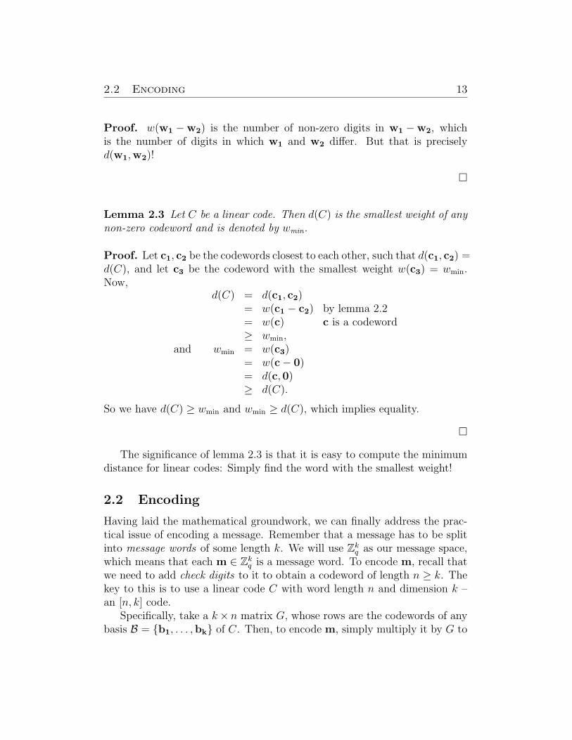
Lemma 2.3 Let C be a linear code. Then d(C) is the smallest weight of anynon-zero codeword and is denoted by wmin.

Proof. Let c1, c2 be the codewords closest to each other, such that d(c1, c2) =d(C), and let c3 be the codeword with the smallest weight w(c3) = wmin.Now,

d(C) = d(c1, c2)= w(c1 − c2) by lemma 2.2= w(c) c is a codeword≥ wmin,

and wmin = w(c3)= w(c− 0)= d(c,0)≥ d(C).

So we have d(C) ≥ wmin and wmin ≥ d(C), which implies equality.

�

The significance of lemma 2.3 is that it is easy to compute the minimumdistance for linear codes: Simply find the word with the smallest weight!

2.2 Encoding

Having laid the mathematical groundwork, we can finally address the prac-tical issue of encoding a message. Remember that a message has to be splitinto message words of some length k. We will use Zk

q as our message space,which means that each m ∈ Zk

q is a message word. To encode m, recall thatwe need to add check digits to it to obtain a codeword of length n ≥ k. Thekey to this is to use a linear code C with word length n and dimension k –an [n, k] code.

Specifically, take a k× n matrix G, whose rows are the codewords of anybasis B = {b1, . . . ,bk} of C. Then, to encode m, simply multiply it by G to

2.2 Encoding 14

get a codeword c ∈ C:

Zkq −→ C ⊆ Zn

q

m 7−→ c := mG =k∑

i=1

mibi

Definition 2.3 A generator matrix for an [n, k] code C is a k × nmatrix G, whose rows are the codewords of any basis of C.

Notice that an [n, k] code C is uniquely defined by a given generatormatrix, though usually it has more than one. Take, for example, the [7, 4]code defined by the generator matrix

G =

1 0 0 0 1 1 10 1 0 0 1 1 00 0 1 0 0 1 10 0 0 1 1 0 1

.

According to the prescribed algorithm, the message word m = (0, 1, 1, 0)under this code is encoded as

c = mG = (0, 1, 1, 0)

1 0 0 0 1 1 10 1 0 0 1 1 00 0 1 0 0 1 10 0 0 1 1 0 1

= (0, 1, 1, 0, 1, 0, 1).

Now take a look at G. Clearly, its four rows are linearly independent and thusconstitute a basis for a code C with dim(C) = 4. This particular generatormatrix, however, has a special feature: It is of the form G = [Ik|A], where Ik

is the k×k identity matrix. Such generator matrices are said to be in standardform, and the advantage of using them is that they leave the message wordintact and simply “add” n − k check digits (here: 1, 0, 1) to it to obtainthe codeword – the process we originally described in chapter 1. For actualdecoders on the other side of the channel, this is a big time-saving featurebecause only the first k digit of each received word need to be checked forerrors. Only if errors are found in the first k digits do we need to examinethe check digits in our decoding process.

2.3 Decoding 15

2.3 Decoding

While encoding is a fairly straightforward process using the generator ma-trix, decoding is not. Oftentimes, a theoretically efficient and powerful error-correcting code cannot be used in practice because there is no good algorithmfor decoding in a feasible amount of time. Recall that the way we decodea received word d is by identifying the closest codeword c. Before we candescribe how to do that, we need to introduce a few more pieces of mathe-matics.

The Parity Check Matrix

A parity check matrix of a code C can be used as a tool to identify whethera received word d is a codeword of C.

Definition 2.4 A parity check matrix for a linear [n, k] code C is a(n− k)× n matrix H that satisfies these two conditions:

i) all of its rows are independent;

ii) cHT = 0 ⇔ c ∈ C.

As we can see from the definition, d is a codeword if and only if theproduct of d and the transpose of H is the zero word. But does every codehave a parity check matrix?

Theorem 2.1 Let C be a [n, k] code with a standard form generatormatrix G = [Ik|A]. Then a parity check matrix for C is H = [−AT |In−k].

Proof. Let the generator matrix of C be

G = [Ik|A] =

1 · · · 0 a11 · · · a1,n−k...

. . ....

......

0 · · · 1 ak1 · · · ak,n−k

,

and let

H = [−AT |In−k] =

−a11 · · · −ak1 1 · · · 0...

. . ....

.... . .

...−a1,n−k · · · −ak,n−k 0 · · · 1

.

2.3 Decoding 16

Is H really a parity check matrix for C? Clearly, H has the right size,namely (n− k)×n, and its rows are independent, so it remains to show thatcHT = 0 ∀ c ∈ C.

Recall that every codeword can be written as c =∑k

i=0 mibi, wheremi ∈ Zq are the message word digits and bi ∈ C are the rows of the generatormatrix. So to get cHT = mibiH

T = 0 we need to ensure that every row ofG is orthogonal to every row of H. But the inner product of the ith row ofG with the jth row of H is

0 + . . . + 0 + (−aij) + 0 + . . . + 0 + aij + 0 + . . . + 0 = 0,

which means that they are indeed orthogonal.

�

So every linear code has a parity check matrix, which can be derived froma generator matrix using the simple formula in theorem 2.1. Going back tothe example in the previous section, the [7, 4] code discussed would have aparity check matrix H below. Notice that in the binary case, −A = A.

H =

1 1 0 1 1 0 01 1 1 0 0 1 01 0 1 1 0 0 1

A parity check matrix is extremely useful. Among many other things, it

allows us to identify the respective code’s minimum distance.

Theorem 2.2 The minimum distance d(C) of a linear code C is thesize of the smallest linearly dependent set of columns of its parity checkmatrix H.

Proof. Let c ∈ C be the codeword with the smallest weight, which iswmin = w(c) = d(C) by lemma 2.3. Then c = (c1, . . . , cn), where all butd(C) digits are zero. Next, let H = [h1 · · ·hn] be the parity check matrixof C, where hi is the ith column of H. Now, by definition of a parity checkmatrix,

cHT = c1h1 + . . . + cnhn = 0,

but only d(C) of the above terms are non-zero. So the size of the triviallydependent set {hi | ci 6= 0} of columns of H is d(C).

2.3 Decoding 17

To show that this is indeed the smallest such set, consider an arbitraryset of t dependent columns: {hσ(1), . . . ,hσ(t)}. By definition of linear depen-dence, there are constants λ1, . . . , λt, not all zero, such that λ1hσ(1) + . . . +λthσ(t) = 0. Now define the word c′ to have the entries λi in its σ(i)th posi-tions and 0 in the remaining positions. Clearly, c′H = 0, so c′ is a codeword,and it is by its definition of weight ≤ t. But t ≥ wmin = d(C), so our originalset {hi | ci 6= 0} of size d(C) is indeed the smallest set of linearly dependentcolumns of H.

�

Hence, to construct a t-error-correcting [n, k] code, it suffices to find an(n− k)× n parity check matrix such that every set of 2t columns is linearlyindependent (recall theorem 1.2).

Finally, let us make one more definition before we go on to show howdecoding is done.

Definition 2.5 Let w be any word and let H be a parity check matrixfor a linear code. Then the syndrome of w is

s(w) := wHT

Cosets and Errors

Let C ⊆ Znq be an [n, k] code. Recall from abstract algebra that the coset of

C associated with the word (element) a ∈ Znq is defined by

a + C = {a + c | c ∈ C}.

Further recall that the word space Znq , consisting of qn words, is partitioned

into a finite number of (non-overlapping) cosets of C. This number, given byLagrange’s Theorem, is |Zn

q |/|C| = qn/qk = qn−k. Now, let d be the receivedword obtained from the original codeword c after the error e occurred: d =c + e Then we have

c = d− e ∈ C

⇒ d + C = e + C.

So since both cosets are the same, it follows that both the received word dand the error word e are in the same coset. However, in a real-world situation

2.3 Decoding 18

we don’t know what e is; we simply receive d. So which word in the cosetd + C is the error that occurred?

Remember, we are using nearest neighbor decoding, which means thatthe original codeword c must be the closest codeword to d: d(d, c) ≤ d(d, c′)for all other codewords c′. In other words, the number of digits in which dand c differ must be minimal. Therefore, the error word e must be the wordin d + C with the smallest weight w(e) possible! So, having received theword d, we can simply go through the coset d + C, find the word with thesmallest weight, which will be our error e, and then correctly decode d asc = d− e.

This type of algorithm, however, though correct, would be enormouslycostly in terms of both running time and storage space. Not only would weneed to store the entire word space Zn

q , its elements ordered by cosets, butwe would also need to browse through this large set in order to find d andthus its coset d + C. Fortunately, there is a better way, which will be pavedby the next two lemmas.

Lemma 2.4 The words v,w belong to the same coset iff s(v) = s(w).

Proof. Let v,w belong to the same coset. Then

v −w ∈ C ⇔ (v −w)HT = 0 ⇔ vHT = wHT ⇔ s(v) = s(w).

�

Lemma 2.5 Let C be a t-error-correcting linear code and let e1, e2 be cor-rectable errors. Then s(e1) 6= s(e2).

Proof. Aiming to get a contradiction, suppose that the two arbitrary errorslie in the same coset: e1+C = e2+C. Then e1 − e2 ∈ C. But w(e1 − e2) ≤2t, because both errors are correctable and thus of weight at most t each.Therefore, using the worst case scenario that their non-zero digits are indifferent positions, we get that their difference must be of weight not morethan 2t. Now,

w(e1 − e2) ≤ 2t< 2t + 1= d(C) by theorem 1.2

But w(e1 − e2) < d(C) is a contradiction because wmin = d(C) by lemma2.3. Therefore, we have e1 + C 6= e2 + C, i.e. no two correctable errors lie inthe same coset. Hence, by the previous lemma 2.4, s(e1) 6= s(e2).

�

2.3 Decoding 19

A Better Decoding Algorithm

Given a t-error-correcting [n, k] code C with a parity check matrix H in stan-dard form, we can use the following algorithm to decode a possibly erroneousreceived word d. First, make a table of all the correctable errors ei (theseare just all the words of weight ≤ t) and their syndromes s(ei) and store it.Then,

1. Calculate s(d) = dHT .

2. Identify the error e in the table as the word with the same syndrome.If none found, d is not decodable by C.

3. Decode to the codeword c = d− e, and drop the last n − k digits toobtain the original message word m.

This algorithm is obviously more efficient than the previously describedscheme because we need to store much less data: merely a table of correctableerrors along with their syndromes. Furthermore, we do not need to look ford, but simply compute its syndrome and then look for the same syndrome ina much smaller list of error syndromes. But why exactly does this algorithmwork?

First, recall that both the error e and the received word d must be in thesame coset. Therefore, by lemma 2.4, they have the same syndrome. Hence,we can simply look up e in the stored table by finding s(e) = s(d), whichwe previously computed. The only thinkable problem would be if two errorshad the same syndrome, and thus the error look-up was not unique. But thisis not the case, as lemma 2.5 asserts. So indeed we have a fast, clean, andmost importantly correct nearest-neighbor decoding algorithm.

We close this section with an example (from [1]) illustrating how to usethis algorithm. Let C be a ternary [7, 3] code with the parity check matrix

H =

1 2 0 1 0 0 01 1 1 0 1 0 00 0 1 0 0 1 02 2 2 0 0 0 1

.

Check that no pair of columns is dependent, but the first, second, and fourthcolumns are since

2

1102

+ 1

2102

+ 2

1000

= 0.

2.4 Hamming Codes 20

Therefore, these three columns constitute the smallest set of dependentcolumns, and so by theorem 2.2, d(C) = 3. From this it follows, by theorem1.2, that C is 1-error-correcting. So t = 1 and thus the correctable errorwords are 0 and all words of weight 1. We construct the error-syndromelook-up table accordingly:

e s(e) e s(e) e s(e)1000000 1102 2000000 2201 0000000 00000100000 2102 0200000 12010010000 0112 0020000 02210001000 1000 0002000 20000000100 0100 0000200 02000000010 0010 0000020 00200000001 0001 0000002 0002

Now suppose that we receive the word d = (1, 0, 1, 0, 1, 2, 2). Simply followthe steps of the algorithm outlined above:

1. s(d) = dHT = (1, 0, 0, 0).

2. In the table we locate (1, 0, 0, 0) as the syndrome of the error e =(0, 0, 0, 1, 0, 0, 0).

3. Therefore, we decode c = d− e = (1, 0, 1, 0, 1, 2, 2)−(0, 0, 0, 1, 0, 0, 0) =(1, 0, 1, 2, 1, 2, 2) ⇒ m = (1, 0, 1, 2).

2.4 Hamming Codes

Despite all the talk about encoding and decoding, we have still not presenteda specific error-correcting code, except partially in the last example. Weshall now discuss one class of codes, the Hamming codes, more in depth.Hamming codes, one of the oldest class of codes, were first implemented inthe 1950s by Richard Hamming, whom we already mentioned in the firstchapter. Though these codes only correct one error per codeword, they doso with great efficiency, and are widely used today in DRAM (main memoryon PCs) error-correction to protect against hardware failure.

Definition 2.6 Let r ≥ 2. A linear code over Zq whose parity checkmatrices have r rows and n columns, where n is the greatest possiblenumber of columns such that no two of them are linearly dependent, iscalled a Hamming Code with redundancy r.


Note that in the binary case q = 2, the condition of column independenceboils down to all columns being distinct and non-zero, for no two distinctnon-zero binary columns can be linearly dependent. The number of distinctbinary columns of length r is 2r, and by subtracting 1 for the 0-column, weget:

n = 2r − 1

in the binary case. The dimension k of the code will therefore be

k = n− r.

From this we can see the natural role for the redundancy r: It is simply thenumber of check digits in a codeword.

We denote the set of all Hamming codes over Zq with redundancy r byHam(r, q). Notice that there are several choices for a code for any givenparameters q, r, but that they all produce similar results, so-called equivalentcodes, which only differ in inessential ways (e.g., one can be obtained from theother by performing a positional permutation on the digits of its codewords).Rather than focusing on these details, however, we will turn our attention towhy the Hamming codes have been such a success.

Theorem 2.3 All Hamming codes are have a minimum distance 3 andthus are 1-error-correcting.

Proof. This directly follows from the definition of a Hamming code inHam(r, q). Since n is the greatest number of columns of its parity checkmatrices consistent with the condition that no two columns are dependent,the size of the smallest set of dependent columns is 3. Therefore, by theorem2.2, d(C) = 3, and so by theorem 1.2, C is 1-error-correcting.

�

Theorem 2.4 All Hamming codes are perfect.

Proof. We need to show that for equality holds with the sphere-packingbound of theorem 1.3 for any Hamming code. Since all Hamming codes are1-error-correcting by the previous theorem, we use t = 1 in our formula:

qn∑1i=0

(ni

)(q − 1)i

=qn

1 + (qr − 1)= qn−r = qk.


But qk is precisely the number of codewords M of a Hamming code becauseits dimension is k. Thus the desired equality holds, and so the code is bydefinition perfect.

�

Even though the Hamming codes are “only” 1-error-correcting, this is notso bad for small codewords and completely sufficient for certain applications.Their strength lies in their obvious simplicity and speed with which code-words can be encoded and decoded. Furthermore, note that all Hammingcodes are 1-error-correcting, no matter what their redundancy is. Redun-dancy should, however, be chosen carefully based on the code’s application,as it greatly affects efficiency. Such issues will be discussed in greater depthin chapter 4.

Again, let us end this last section with a hopefully illuminating example,the already mentioned Hamming(7,4) code in Ham(3, 2). Since this is abinary code, a parity check matrix can be constructed by simply listing allthe 23 − 1 = 7 distinct non-zero binary columns of length 3. To get thematrix in standard form, let the last three columns for the identity matrixI3. One possible parity check matrix is

H =

1 1 0 1 1 0 01 1 1 0 0 1 01 0 1 1 0 0 1

.

From this, we get the generator matrix using theorem 2.1:

G =

1 0 0 0 1 1 10 1 0 0 1 1 00 0 1 0 0 1 10 0 0 1 1 0 1

.

Suppose Alice wants to send Bob the message word m = (1, 0, 0, 1). Shewill encode it as c = mG = (1, 0, 0, 1, 0, 1, 0). Now suppose an error in thethird digit occurs, and Bob receives d = (1, 0, 1, 1, 0, 1, 0). He will computes(d) = dHT = (0, 1, 1). In the error-syndrome lookup table (not picturedhere), he will find that e = (0, 0, 1, 0, 0, 0, 0), and thus correctly decode toc = (1, 0, 0, 1, 0, 1, 0) ⇒ m = (1, 0, 0, 1).

23

3 Cyclic Codes

Cyclic codes are a subclass of linear codes that have an additional conditionimposed upon them – the cyclic property, which we will discuss shortly.The advantage of cyclic codes is that their codewords can be represented aspolynomials – as opposed to vectors – over a finite field (again, usually overZ2). Whereas the language of the linear block codes discussed in the previouschapter is linear algebra, cyclic code properties are generally phrased in termsof ring theory. The reader will, however, notice many similarities, as most ofthe concepts are analogous.

The Hamming codes from section 2.4 turn out to be cyclic in fact, thoughwe will not discuss this representation here. Instead, we will present thecyclic version of the binary Golay Code, which is capable of correcting 3errors per word. We will also briefly introduce the so-called Fire Codes,which are especially efficient at correcting errors that occur in bursts ratherthan randomly.

3.1 Polynomial Code Representation

Let us first consider a regular linear code C with codeword length n. Thecrucial idea here is that of a cyclic shift. If c = (c0, . . . , cn−1) ∈ C, then thecyclic shift of c is defined as

C(c) = (cn−1, c0, . . . , cn−2).

C shifts all digits to the right by one and places the last digit in the firstposition. Using this notation, we now define a special class of linear codes.

Definition 3.1 A linear code C is called a cyclic code if and only if

c ∈ C ⇒ C(c) ∈ C.

On a first glance, this cyclic property for linear codes seems rather arbitraryand not very useful. Its significance will become apparent, however, whenwe change our word space.

So far, we have represented words as vectors in Znq , a vector space over a

finite field. This turned out to be a convenient representation, but let’s trysomething different now. Let us identify the word w of length n with thepolynomial of degree n− 1, whose coefficients are the digits of w:

w = (w0, w1, . . . , wn−1) 7−→ w(x) = w0 + w1x + . . . + wn−1xn−1

3.1 Polynomial Code Representation 24

The motivating reason for this polynomial representation is that cyclic shiftsare particularly easy to perform. Specifically, notice what happens when wemultiply a word w(x) =

∑n−1i=0 wix

i by x:

x · w(x) = w0x + w1x2 + . . . + wn−2x

n−1 + wn−1xn

≡ wn−1 + w0x + w1x2 + . . . + wn−2x

n−1 (mod xn − 1)

= C(w(x)).

So if we take as our word space the quotient ring

Rn := Zq[x]/(xn − 1),

whose elements we will regard simply as polynomials of degree less than nrather than their equivalence classes, then multiplying a word by x corre-sponds to a cyclic shift of that word. Similarly, multiplying by xm corre-sponds to a m cyclic shifts (a shift through m positions).

In this new setting, there is an algebraic characterization of cyclic codesthat is quite similar to the definition (2.1) of linear codes.

Theorem 3.1 A code C is cyclic if and only if it is an ideal in Rn, i.e.

i) 0 ∈ C

ii) c1(x), c2(x) ∈ C ⇒ c1(x) + c2(x) ∈ C

iii) r(x) ∈ Rn, c(x) ∈ C ⇒ r(x)c(x) ∈ C

Proof. First, suppose that C is a cyclic code, as defined by definition 3.1.(i) Since C is a linear code, the zero word is one of its elements.(ii) Similarly, by def. 3.1, the sum of two codewords is again a codeword.(iii) Let r(x)c(x) = r0c(x) + r1(xc(x)) + . . . + rn−1(x

n−1c(x)). Noticethat in each summand, the codeword c(x) is first cyclically shifted by theaccording number of positions, and then multiplied by a constant ri ∈ Zq.But both of these operations, as well as the final addition of summands, areclosed in C by its definition as a linear code, so we indeed have r(x)c(c) ∈ C.

Conversely, suppose that C is an ideal in Rn, and thus (i),(ii),(iii) hold.If we take r(x) to be a scalar in Zq, these conditions imply that C is a linearcode by definition 2.1. If we take r(x) = x, (iii) implies that C is also cyclic.

�

3.2 Encoding 25

3.2 Encoding

Just as linear block codes were constructed using a generator matrix G, cycliccodes can be constructed using a generator polynomial, denoted by g(x). Butbefore we introduce it by its name, let us look at some of the properties ofthis polynomial.

Theorem 3.2 Let C be a non-zero cyclic code in Rn. Then

i) there exists a unique monic polynomial g(x) ∈ C of smallest degree;

ii) the code is generated by g(x): C = 〈g(x)〉;

iii) g(x) is a factor of (xn − 1).

Proof.(i) Clearly, since C is not empty, a smallest degree polynomial g(x) must

exist. If it is not monic, simply multiply it by a suitable scalar. Now sup-pose it was not unique, that is, suppose there are two monic polynomialsg(x), h(x) ∈ C of smallest degree. Then g(x) − h(x) ∈ C, again multipliedby a suitable scalar, is monic and of a smaller degree than deg(g(x)), whichis a contradiction.

(ii) Let c(x) ∈ C, and divide it by g(x). By the division algorithm, we getc(x) = q(x)g(x) + r(x), where deg(r(x)) < deg(g(x)). Now, c(x), g(x) ∈ Cand q(x) ∈ Rn. Since C is an ideal, we can conclude that r(x) = c(x) −q(x)g(x) ∈ C. But since we said that g(x) is the smallest degree polynomialin C, the only possibility for the remainder is r(x) = 0. Hence, c(x) =q(x)r(x) for any codeword in C, so we must have c(x) ∈ 〈g(x)〉 and thusC = 〈g(x)〉.

(iii) Again, by the division algorithm, xn − 1 = q(x)g(x) + r(x), wheredeg(r(x)) < deg(g(x)). But r(x) ≡ −q(x)g(x) (mod xn − 1), so r(x) ∈〈g(x)〉 = C. By the minimality of deg(g(x)), we must again have r(x) = 0.So xn − 1 = q(x)g(x), which means that g(x) is a factor of xn − 1.

�

Definition 3.2 The generator polynomial of a cyclic code C is theunique monic polynomial g(x) ∈ C of smallest degree.

Theorem 3.2 tells us that such a polynomial (i) exists and is unique, (ii) is

3.2 Encoding 26

indeed a generator of C in the algebraic sense, and (iii) can be found byfactoring the modulus (xn − 1). The following table (taken from [2]) showssome of these factorizations for small n:

n factorization of (xn − 1) over Z2

1 (1 + x)2 (1 + x)2

3 (1 + x)(1 + x + x2)4 (1 + x)4

5 (1 + x)(1 + x + x2 + x3 + x4)6 (1 + x)2(1 + x + x2)2

7 (1 + x)(1 + x + x3)(1 + x2 + x3)8 (1 + x)8

Now the natural question becomes: Which of the factors of xn− 1 should wepick as a generator polynomial? The answer depends on what we want thedimension of our code to be. The following theorem clarifies this.

Theorem 3.3 Let C be a cyclic code of codeword length n and let g(x) =g0 + g1x + . . . + grx

r be its generator polynomial of degree r. Then agenerator matrix for C is the (n− r)× n matrix

G =

g0 g1 · · · gr 0 · · · 0

0 g0 g1 · · · gr...

.... . . . . . . . . 0

0 · · · 0 g0 g1 · · · gr

and therefore k := dim(C) = n− r.

Proof. First, it is important to note that g0 6= 0. Suppose it were; theng(x) = g1x+ . . .+grx

r and since C is cyclic, xn−1g(x) = x−1g(x) = g1 + . . .+grx

r−1 ∈ C would also be a codeword, but of degree r− 1, which contradictsthe minimality of deg(g(x)) = r.

So the constant coefficient g0 is indeed non-zero. It follows that the rowsof the matrix G are linearly independent because of the echelon of g0’s. Itremains to show that the rows constitute a basis of C, i.e. that any codewordcan be expressed as a linear combination of these rows, which represent thecodewords g(x), xg(x), x2g(x), . . . , xn−r−1g(x).

By theorem 3.3 part (ii), we already know that any codeword c(x) can bewritten in the form c(x) = q(x)g(x), for some word q(x). Now, deg(c(x)) <

3.3 Decoding 27

n ⇒ deg(q(x)) < n− r, and thus we can write

c(x) = q(x)g(x)

= (q0 + q1x + . . . + qn−r−1xn−r−1)g(x)

= q0[g(x)] + q1[xg(x)] + . . . + qn−r−1[xn−r−1g(x)]

which is indeed a linear combination of the rows of G. Therefore, the linearlyindependent rows are a basis for C, and so by definition 2.3, G is a generatormatrix for this code.

�

Let us look at the simple case of binary cyclic codes of codeword length 3.From the factorization table above we can see that (x3−1) = (1+x)(1+x+x2). If we want a code with dimension k = 2, then we must pick as generatorpolynomial the factor with degree r = 3 − 2 = 1, which is 1 + x. We thenget the following generator polynomial g(x), generator matrix G, and cycliccode C:

g(x) = 1 + x, G =

[1 1 00 1 1

], C = {000, 011, 110, 101}.

On the other hand, if we want a code with dimension 1, we get

g(x) = 1 + x + x2, G =[

1 1 1], C = {000, 111}.

3.3 Decoding

The reader will probably have noticed that the generator matrix G we con-structed is not in standard form, so we cannot use the method from theorem2.1 to find a parity check matrix H. Nevertheless, there is a very naturalchoice for H, much like there was for G.

Definition 3.3 Let C be an cyclic [n, k] code with the degree r generatorpolynomial g(x). Then a check polynomial for C is the degree k = n−rpolynomial h(x) such that

g(x)h(x) = xn − 1

Notice that since g(x) is a factor of xn − 1 by theorem 3.2 part (iii), h(x)must exist: It is the “other” factor of xn − 1, which corresponds to 0 in Rn.

3.3 Decoding 28

Furthermore, since g(x) is by definition monic, h(x) must be monic also, forelse we would not get the coefficient 1 for xn in their product. Finally, thename check polynomial was not chosen at random; h(x) has some familiarproperties reminiscent of the parity check matrix H.

Theorem 3.4 Let C be a cyclic code in Rn with the generator and checkpolynomials g(x) and h(x), respectively. Then

c(x) ∈ C ⇔ c(x)h(x) = 0.

Proof. First, suppose that c(x) ∈ C. Since C = 〈g(x)〉, we have

c(x) = a(x)g(x) for some a(x) ∈ Rn

⇔ c(x)h(x) = a(x)g(x)h(x) multiply by h(x)= a(x)(xn − 1) by definition of h(x)≡ a(x) · 0 in Rn

= 0 as desired.

Conversely, suppose that c(x)h(x) = 0. If we divide c(x) by g(x), thenby the division algorithm, c(x) = q(x)g(x) + r(x), where deg(r(x)) < n− k.So we get

r(x) = c(x)− q(x)g(x)

⇔ r(x)h(x) = c(x)h(x)− q(x)g(x)h(x)

= 0− 0 = 0 by def. of h(x) and assumption.

Note that in Rn this really means r(x)h(x) ≡ 0 (mod xn − 1). But we have

deg(r(x)h(x)) = deg(r(x)) + deg(h(x))

since these are polynomials over Zq, a finite field. So, deg(r(x)h(x)) < (n−k)+k = n, which means that we really have r(x)h(x) = 0 in Zq[x]. Therefore,the only possibility is r(x) = 0, since h(x) is clearly non-zero. Hence, c(x) =q(x)g(x) ∈ 〈g(x)〉 = C.

�

Just as we could express the generator matrix using the generator poly-nomial, we can express the parity check matrix using the check polynomialin much the same way.

3.3 Decoding 29

Theorem 3.5 Let C be an [n, k] cyclic code with the check polynomialh(x) = h0 + h1x + . . . + hkx

k. Then a parity check matrix for C is

H =

hk hk−1 · · · h0 0 · · · 0

0 hk hk−1 · · · h0...

.... . . . . . . . . 0

0 · · · 0 hk hk−1 · · · h0

Proof. We know that h(x) is a monic polynomial and therefore hk = 1, sothe hk’s form an echelon in H and thus its rows are linearly independent.We still need to show that cHT = 0 for all c ∈ C.

Let c = (c0, c1, . . . , cn−1), which corresponds to c(x) = c0 + c1x + . . . +cn−1x

n−1, be any codeword of C. By the definition of h(x), we have c(x)h(x) =0. If we write this out carefully, we see that

c(x)h(x) = (c0 + c1x + . . . + cn−1xn−1)(h0 + h1x + . . . + hkx

k)

= c0h0 + . . .

+(c0hk + c1hk−1 + . . . + ckh0)xk

+(c1hk + c2hk−1 + . . . + ck+1h0)xk+1 + . . .

+(cn−k−1hk + cn−khk−1 + . . . + cn−1h0)xn−1

= 0

implies in particular that each of the coefficients of xk, . . . , xn−1 must be 0:

c0hk + c1hk−1 + . . . + ckh0 = 0

c1hk + c2hk−1 + . . . + ck+1h0 = 0...

cn−k−1hk + cn−khk−1 + . . . + cn−1h0 = 0

But notice that this is precisely equivalent to saying that cHT = 0, which iswhat we wanted to show.

�

Instead of talking about the generalities of how to encode and decodewith cyclic codes, how to find their minimum distance, etc., we will focus ontwo specific cyclic codes, which have proved to be very useful and effective.This will be the topic of the next two sections.

3.4 The Binary Golay Code 30

3.4 The Binary Golay Code

The binary Golay code, though not of much practical use anymore due toinnovation in coding, is quite interesting from a mathematical point of viewas it leads into related mathematical topics such as group theory and combi-natorics (see [3], for instance). That is not to say that it is completely useless,however. It was successfully used in the 1970s on the Voyager 2 spacecraftduring its Mission to Jupiter and Saturn, and it is in fact one of the oldestknown error-correcting codes. The Golay code is perfect just like the Ham-ming codes, yet has a greater minimum distance and thus error-correctingcapability. It should be noted that there are different ways of constructingthe binary Golay code; we will do so via polynomials, since that is the topicof this chapter.

We start by introducing some terminology and an important result. Iff(x) = a0 +a1x+ . . .+anx

n is a polynomial in Rn, then f(x) = an +an−1x+. . . + a0x

n is called the reciprocal of f(x). Using this notation, we state animportant fact:

Lemma 3.1 Let xp − 1 = (x − 1)g(x)g(x), where p is a prime, and letc(x) ∈ 〈g(x)〉 be a codeword of weight w. Then:

i) w2 − w ≥ p− 1 if w is odd;

ii) w ≡ 0 (mod 4) and w 6= 4 unless p = 7 if w is even.

For a proof of this general result please refer to [1] pp 153-155 or [4] pp 154-156. The discussion is relatively lengthy and not necessary for understandingthe rest of this section.

Let us consider the case where p = 23, where we get the following factor-ization (over Z2):

(x23 − 1) = (x− 1)

·(x11 + x10 + x6 + x5 + x4 + x2 + 1)

·(x11 + x9 + x7 + x6 + x5 + x + 1)

=: (x− 1)g(x)g(x).

Notice that the two degree 11 polynomials are indeed reciprocals. Next,consider the code generated by g(x).

3.5 Burst Errors and Fire Codes 31

Definition 3.4 The binary cyclic code in R23 with generator polynomialg(x) = 1+x2 +x4 +x5 +x6 +x10 +x11 is called the binary Golay Code,denoted by G23.

With the help of the previous lemma, we will now prove the crucial prop-erty of the Golay code.

Theorem 3.6 G23 is a perfect three-error-correcting [23, 12] code.

Proof. By theorem 3.3, G23 is a [23, 12] code because its generator g(x)of degree 11 is a product of x23 − 1, as shown above. Let c(x) ∈ G23 be acodeword with minimum weight wmin. If this weight is odd, then by lemma3.1.(i) we must have

w2min − wmin ≥ 23− 1

⇒ wmin(wmin − 1) ≥ 22⇒ wmin ≥ 7. (try it!)

On the other hand, lemma 3.1.(ii) implies that G23 has no words of evenweight < 8, because p = 23 6= 7. Finally, we can see that w(g(x)) = 7, sothe minimum distance d(G23) = 7. By theorem 1.2, the binary Golay codeis therefore 3-error-correcting.

It remains to show the G23 is perfect. Checking the sphere packing bound(theorem 1.3) for t = 3, we get:

223∑3i=0

(23i

)(2− 1)i

=223

1 + 23 + 23·222

+ 23·22·216

=223

1 + 23 + 253 + 1771

=223

2048=

223

212= 211

which is exactly 2k, the number of codewords M , and thus G23 is perfect.

�

3.5 Burst Errors and Fire Codes

So far, we have not addressed the issue of what types of errors occur in a noisychannel. We have simply assumed that errors, in the form of binary digit


changes, occur randomly throughout a message with some small, uniformlydistributed probability for any given digit. Our only criterion for a code’serror-correcting capability so far is its minimum distance, from which we cantell how many errors per codeword can be corrected. However, if we knowthat only certain types of errors will occur, we can greatly improve our codingefficiency (in terms of information rate).

Among particularly common types of errors are so-called burst errors. Aburst error e of length t is simply an error in t consecutive codeword digits:

e = (0, . . . , 0, 1, . . . , 1︸︷︷︸t digits

, 0, . . . , 0)

As a polynomial, a burst error can be expressed as

e(x) = xib(x) = xi(b0 + b1x + . . . + bt−1xt−1)

i.e. a cyclic shift by i digits of a polynomial b(x) with deg(b(x)) = t− 1 andnon-zero coefficients bj. Such errors often occur in digital data storage devicessuch as CDs, for example, where physical scratches and other distortions areusually the cause. It turns out that burst errors can be corrected with muchless overhead than random errors of the same size.

The Fire codes, originally discovered by P. Fire in 19592, are one classof such burst-error-correcting codes. In fact, these codes are considered tobe the best single-burst-correcting codes of high transmission rate known,according to [5].

Definition 3.5 A Fire Code of codeword length n is a cyclic code inRn with generator polynomial

g(x) = (x2t−1 − 1)p(x)

where p(x) is an irreducible polynomial over Zq that does not divide(x2t−1 − 1) and with m := deg(p(x)) ≥ t, and n is the smallest inte-ger such that g(x) divides (xn − 1).

For example, the [105, 94] code with generator polynomial g(x) = (1 +x7)(1 + x + x4) is a Fire code, but notice that a Fire code need not (andusually does not) exist for any given n. Nevertheless, it turns out that the

2see [10]


number t in the definition above is precisely the maximum correctable burstlength.

Lemma 3.2 A Fire code has codeword length n = lcm(2t− 1, qm − 1).

Proof. Let us denote g(x) = a(x)p(x), where a(x) = x2t−1 − 1. We want nto be the smallest integer such that g(x) | (xn−1). But by definition, p(x) isirreducible and does not divide a(x), which implies that gcd(a(x), p(x)) = 1.Therefore,

a(x) | (xn − 1)

and p(x) | (xn − 1)

imply that g(x) | (xn − 1), so we will find the smallest n that satisfies thesetwo conditions.

The smallest integer e for which p(x) | (xe − 1) is e = qm − 1, wherem = deg(p(x)). Clearly, e | lcm(2t− 1, e), so (xe − 1) | (xlcm(2t−1,e) − 1). But

p(x) | (xe − 1) and (xe − 1) | (xlcm(2t−1,e) − 1) ⇒ p(x) | (xlcm(2t−1,e) − 1).

On the other hand, (2t− 1) | lcm(2t− 1, e), so

(x2t−1 − 1)) | (xlcm(2t−1,e) − 1) ⇔ a(x) | (xlcm(2t−1,e) − 1).

Therefore, (1) and (2) are satisfied by n = lcm(2t−1, e) = lcm(2t−1, qm−1),and since this is the least common multiple, they cannot by satisfied by anysmaller n.

�

Theorem 3.7 A Fire code can correct all burst errors of length t or less.

Proof. We base our argument on the presentation in [11], pp 480-481. Letd(x) = c(x) + e(x) be the received word, where c(x) is the original Fire codecodeword and e(x) = xib(x) is a burst error of length t or less. We want toshow that we can uniquely identify this burst error given only our receivedword d(x). In order to do that, we need to find

• the burst pattern b(x) of length ≤ t and thus degree ≤ t− 1, and

• the position i of this burst pattern in a word of length n.


Since i < n, it suffices to find i (mod n). But by lemma 3.2, n = lcm(2t −1, qm − 1), so it suffices to find i (mod 2t− 1) and i (mod qm − 1).

First, let us find b(x) and i (mod 2t− 1). Define

s1(x) := d(x) (mod x2t−1 − 1)= c(x) + e(x) (mod x2t−1 − 1)= e(x) (mod x2t−1 − 1) because c(x) is a multiple of g(x),

which is a multiple of x2t−1 − 1= xib(x) (mod x2t−1 − 1).

Since n is a multiple of 2t− 1, our error word will look like this:

e(x) = (

2t−1︷︸︸︷0, . . . , 0,

2t−1︷︸︸︷0, . . . , 0, . . . ,

2t−1︷︸︸︷0, . . . , 1, . . . , 1︸︷︷︸

b(x) at position i

, . . . , 0, . . . ,

2t−1︷︸︸︷0, . . . , 0)

Taking this burst error modulo (x2t−1 − 1) will simply reduce all exponentsto values less than 2t − 1, and shift the burst pattern into the first 2t − 1digits without changing it:

s1(x) = (

2t−1︷︸︸︷0, . . . , 0, 1, . . . , 1︸︷︷︸

b(x) at position i′

, 0, . . . , 0).

Here, i′ := i (mod 2t − 1), and so we have s1(x) ≡ xi′b(x) (mod x2t−1 − 1),where both b(x) and i′ are uniquely determined by the received word d(x).Thus we have found the burst pattern b(x) and its position i (mod 2t− 1).

It remains to show that i (mod qm − 1) is uniquely determined as well.To that end, write

i = i′ + k(2t− 1)

for some multiple k < n2t−1

. We already know i′, so we only need to find

k(2t − 1) (mod qm − 1). In other words, we need k (mod qm−1gcd(2t−1,qm−1)

).Define

s2(x) := d(x) (mod p(x))= c(x) + e(x) (mod p(x))= e(x) (mod p(x)) because c(x) is a multiple of g(x)

which is a multiple of p(x)= xib(x) (mod p(x))= xi′+k(2t−1)b(x) (mod p(x))= q(x)p(x) + xi′+k(2t−1)b(x) for some polynomial q(x).


Now let α ∈ F×qm be a root of p(x), which must have order e = qm − 1, for

that is the smallest integer for which p(x) divides xe − 1 (recall lemma 3.2).Then

s2(α) = q(α) · 0 + αi′+k(2t−1)b(α),

and since p(x) is irreducible and deg(b(x)) < t ≤ m = deg(p(x)), we haveb(α) 6= 0, and so

αi′+k(2t−1) =s2(α)

b(α).

Now we can use this equation to find k (mod qm−1gcd(2t−1,qm−1)

). First we computethe right-hand side and then we match the exponent to the left-hand side,where α is a generator of the cyclic group F×

qm .Hence, we have found all that we needed to recover the burst error e(x) =

xib(x) of length t or less from any received word d(x). Therefore, the Firecodes are indeed t-burst-error-correcting.

�

An alternative proof of theorem 3.7 can be found in texts such as [5].Having established the error-correcting capabilities of Fire codes, we will nexttest the performance of the Fire code with t = 3 and see how it measures upto the other codes we have discussed. This will be the topic of the subsequent,final chapter.

36

4 Code Performance

This final chapter is very different from the previous ones in that we do notintroduce any new theory. Instead, the sole focus will be on the performanceof the three classes of codes we have described so far – the Hamming codes,the binary Golay code, and the Fire codes – given different types and fre-quencies of errors. To this end, we have used a test program that implementsthese various codes and tests their error-correcting capabilities.

The first section discusses some of the implementation details of thisprogram. The next section fully describes the performance test and presentsthe data obtained from it. The final section then discusses several highlightsin the results and compares the test data to theoretically expected values.

Although there is by no means any scientific breakthrough here, the testresults we discuss here are nevertheless interesting in so far as they high-light the inverse relationship between a code’s error-correcting capability (asmeasured by its correction rate) and coding efficiency (as measured by itsinformation rate). Finding new codes with a higher error-correcting capabil-ity while maintaining efficiency and keeping implementation overhead low isan area of ongoing research.

4.1 Implementation Issues

The program used to test code performance was written in Java. Hence, itwas natural to approach the problem from an object-oriented point of view.

There is a Word class for binary words, which stores the digits of theword in an array, along with the word’s length and weight. In addition,the class implements the addition and scalar product of two words. Allcoding operations in the program are done in terms of Word objects, whichin particular implies that all codes are binary.

A Code class is used as a template for a generic linear error-correctingcode with codeword length n, dimension k, redundancy r, generator matrixG, and parity check matrix H. In addition, a table of correctable errors hashedby their syndromes, such as the one from our example in section 2.3, is stored.The methods for encoding and decoding are implemented in this class as well.

Extending the Code class are the Hamming and Cyclic classes, each ofwhich implements a constructor for the particular kind of code desired. Thejob of the constructor is to build appropriate generator and parity checkmatrices as well as an error table for some given input parameters.

The only parameter for the Hamming constructor is an integer r for the

4.1 Implementation Issues 37

code redundancy, which is stored as r. All other information can be derivedfrom r, as discussed in section 2.4:

• n = 2r − 1

• k = n− r

• H is the r×n matrix whose columns are all the non-zero binary wordsof length r, arranged in the standard form H = [A|Ir];

• G is the k × n matrix [Ik|AT ] (by theorem 2.1 - binary case);

• The error table contains all errors of weight 1 (plus the zero word) sinceall codes in Ham(r, 2) are 1-error-correcting.

An interesting real-world implementation issue is the question of how toefficiently generate the columns of H. In other words, we want to generateall the distinct non-zero binary words of length r. A nice way to do thatis to use a Gray Code3, which is a method of listing all binary words of agiven length in an order such that not more than one digit changes fromone word in the list to the next. For example, compare the “standard” wayof listing consecutive binary integers of length 3 in ascending order to thecorresponding Gray Code:

02 − 72 Gray Code000 000001 001010 011011 010100 110101 111110 101111 100

The digits that have changed from one word to the next are highlighted onboth sides. Note that while only one digit changes in the Gray Code, upto all three digits change in the left column. For this reason, the Hamming

class uses a Gray Code when constructing the parity check matrix (a specialGrayCode class was written for this).

The Cyclic constructor needs significantly more information than justredundancy to construct a cyclic code. Its input parameters are the codeword

3see e.g. [9]

4.2 Test Description and Results 38

length n, a generator polynomial g(x) and a check polynomial h(x). Usingthis information, the desired Cyclic code object is built.

4.2 Test Description and Results

We tested the following six error-correcting codes for their performance. Notethat they are all linear [n, k] codes.

1. H7: A Hamming [7, 4] code with redundancy 3.




5. G23: The binary Golay [23, 12] code with generator polynomialg(x) = 1 + x2 + x4 + x5 + x6 + x10 + x11.

6. F35: The [35, 27] Fire code with generator polynomialg(x) = (x2·3−1−1)p(x) = (1+x5)(1+x+x3) = 1+x+x3 +x5 +x6 +x8.

We have seen that the Hamming codes are all 1-error-correcting, the Golaycode is 3-error-correcting, and this particular Fire code can correct all bursterrors up to burst length t = 3. Table 1 below lists the codes’ respectiveinformation rates. Recall that ρ = 1

nlogq M , and in all cases we have M = qk

(by lemma 2.1) and q = 2.The test is then conducted as follows. First, an arbitrary message con-

sisting of 10,000 bits is encoded into codewords for each of the six codes.Then, one of the following two types of errors is introduced throughout theentire message:

• A random error pattern, where the probability that any given code-word digit ci gets corrupted is p. In other words, the probability of eacherror word of weight 1 (of the form 0...010...0) occurring is p. Note,however, that it is possible that more than one such error occurs percodeword. This is obviously more likely when codewords are longer.

• A burst error pattern, where the probability that a burst of length 3occurs starting at any given digit ci is p. In other words, the probabilityof each burst error word of weight 3 (of the form 0...01110...0)occurring is p. Notice that in this scenario, it is possible that bursts of


length greater or less than three appear as a result of the conceivableevent of two or more bursts in one codeword (burst error underlined):

1101000b1=0111000−→ 1010000

b2=0000111−→ 1010111, vs.

1101000b1=0111000−→ 1010000

b2=0011100−→ 1000100.

Once the errors are introduced, the possibly erroneous words are decoded,and the program checks how many of these words have been decoded cor-rectly, i.e. restored to their original codewords. We call the percentage ofreceived words that has been correctly decoded the correction rate, denotedby R. This measure of error-correcting capability is computed for each ofthe six codes for different values of p, ranging from 0 to 0.06. The process isrepeated 30 times (for accuracy) and mean values of R are reported. The re-sults of this test are presented in figures and tables 2 and 3 on the subsequentpages.

TABLE 1. Information rates.

code H7 H15 H31 H63 G23 F35

ρ 57.142% 73.333% 83.871% 90.476% 52.174% 77.143%


Figure 2: Code performance, given the random error pattern described.

Figure 3: Code performance, given the burst error pattern described.


TABLE 2. Data for the random error pattern in figure 2.

p H7 H15 H31 H63 G23 F35

0.000 100.000% 100.000% 100.000% 100.000% 100.000% 100.000%0.002 99.992% 99.969% 99.823% 99.318% 100.000% 99.827%0.004 99.968% 99.835% 99.423% 97.261% 100.000% 99.191%0.006 99.918% 99.624% 98.499% 94.205% 99.998% 98.156%0.008 99.863% 99.363% 97.512% 90.909% 100.000% 97.084%0.010 99.804% 99.066% 96.114% 86.943% 99.986% 95.321%0.012 99.722% 98.626% 94.805% 82.682% 99.981% 93.822%0.014 99.607% 98.158% 92.758% 77.648% 99.990% 91.369%0.016 99.498% 97.640% 91.429% 72.898% 99.952% 89.806%0.018 99.381% 96.993% 89.205% 69.136% 99.930% 87.542%0.020 99.258% 96.499% 87.055% 64.045% 99.921% 85.062%0.022 99.039% 95.752% 84.592% 59.955% 99.878% 83.084%0.024 98.903% 95.042% 83.164% 54.966% 99.799% 80.119%0.026 98.660% 94.196% 80.618% 50.898% 99.765% 78.151%0.028 98.503% 93.327% 78.660% 47.068% 99.669% 75.391%0.030 98.294% 92.811% 76.530% 42.716% 99.525% 73.488%0.032 98.054% 91.932% 73.564% 40.045% 99.465% 70.588%0.034 97.869% 90.930% 72.083% 36.580% 99.314% 67.741%0.036 97.566% 90.068% 68.748% 33.182% 99.062% 64.997%0.038 97.404% 88.905% 66.914% 30.625% 98.945% 63.321%0.040 96.988% 88.075% 64.935% 27.614% 98.727% 60.620%0.042 96.811% 86.866% 62.431% 24.773% 98.532% 58.092%0.044 96.554% 86.123% 59.725% 23.023% 98.305% 55.332%0.046 96.204% 85.167% 58.151% 21.102% 97.964% 53.499%0.048 95.910% 84.143% 55.548% 18.977% 97.830% 50.846%0.050 95.499% 82.752% 54.390% 16.875% 97.456% 48.739%0.052 95.236% 81.712% 51.003% 15.614% 97.079% 46.965%0.054 94.806% 80.692% 49.538% 13.886% 96.751% 44.253%0.056 94.576% 79.393% 47.434% 11.898% 96.403% 42.863%0.058 94.170% 78.473% 45.210% 11.727% 95.986% 40.749%


TABLE 3. Data for the burst error pattern in figure 3.

p H7 H15 H31 H63 G23 F35

0.000 100.000% 100.000% 100.000% 100.000% 100.000% 100.000%0.002 98.606% 97.059% 93.735% 88.477% 99.926% 99.779%0.004 97.334% 94.244% 87.906% 77.182% 99.624% 99.089%0.006 95.808% 91.327% 83.117% 68.693% 99.108% 97.914%0.008 94.597% 88.629% 78.255% 60.170% 98.345% 96.415%0.010 93.225% 86.097% 73.060% 53.080% 97.683% 94.706%0.012 91.933% 83.429% 68.894% 45.761% 96.715% 92.814%0.014 90.750% 80.998% 64.732% 41.602% 95.667% 90.566%0.016 89.416% 78.347% 60.992% 36.261% 94.552% 87.903%0.018 88.155% 76.347% 57.294% 32.398% 93.333% 85.569%0.020 87.025% 73.593% 53.740% 28.705% 92.007% 83.445%0.022 85.664% 71.771% 50.566% 23.977% 90.451% 80.431%0.024 84.419% 69.554% 47.060% 21.636% 89.432% 77.784%0.026 83.373% 67.464% 44.930% 18.523% 87.777% 75.111%0.028 82.110% 65.503% 41.673% 17.523% 86.046% 72.162%0.030 81.290% 63.532% 38.997% 15.034% 84.072% 69.040%0.032 79.966% 61.224% 36.499% 13.307% 82.350% 66.776%0.034 78.681% 60.404% 34.919% 11.102% 81.048% 64.210%0.036 77.692% 57.954% 31.953% 9.295% 79.245% 61.687%0.038 76.766% 56.270% 29.860% 8.125% 77.213% 59.224%0.040 75.559% 54.501% 27.600% 7.591% 75.957% 56.582%0.042 74.409% 52.952% 26.831% 6.852% 73.847% 54.059%0.044 73.311% 51.066% 25.143% 5.466% 72.089% 50.658%0.046 72.502% 49.798% 23.616% 5.307% 70.276% 48.809%0.048 71.272% 47.956% 21.881% 4.330% 68.662% 47.067%0.050 70.402% 47.068% 20.660% 3.489% 67.168% 44.361%0.052 69.531% 45.459% 19.506% 3.670% 65.643% 42.097%0.054 68.352% 43.690% 18.343% 3.330% 63.633% 39.655%0.056 67.334% 42.338% 16.919% 2.614% 61.739% 38.852%0.058 66.566% 41.365% 16.156% 2.193% 60.345% 36.081%

4.3 Conclusions 43

4.3 Conclusions

First, we observe that the experimental data is quite close to theoreticalexpected values. Take, for example, p = 0.02 in the random error pattern.Now consider, say, the Hamming code H31, which is a 1-error-correcting code.The probability that one error or less occurs per codeword is

1∑i=0

(31

i

)0.02i0.9831−i = 0.9831 + 31 · 0.02 · 0.9830 = 87.277%

which is close to its measured error-correcting capability, 87.055% (see table2). As another example, consider the 3-error-correcting Golay code G23. Itsexpected error-correcting capability is∑3

i=0

(23i

)0.02i0.9823−i

= 0.9823 + 23 · 0.02 · 0.9822 + 253 · 0.022 · 0.9821 + 1771 · 0.023 · 0.9820

= 99.896%

as compared to the measured 99.921%. These sample calculations indicatethat the test went as it was intended.

Next, we make some qualitative observations, and note that the resultswe got in figures 2 and 3 should not be very surprising. The graphs clearlyshow that a code’s correction rate R decreases as the error rate p increases –this makes perfect sense. Furthermore, as figure 2 unambiguously illustrates,the general trend is that increasing error-correcting capability carries with itan explicit cost in terms of efficiency.

For example, on a first glance G23 might seem like the best code becauseof its consistently highR value. But a look at table 1 reveals that it is also theleast efficient, with its information rate at only 52%. In fact, by comparingtable 1 and figure 2, we can see that the higher a code is on the graph (thegreater its R), the lower is its efficiency ρ – with the sole exception of F35,which performs marginally worse than H31, despite lower efficiency.

That is not to say, however, that F35 is a particularly poorly performingcode. On the contrary, it proves to perform significantly better relative toother codes when faced with the types of burst errors it was designed for,as can be seen in figure 3. Its performance is especially strong for small p,as this decreases the probability of more than one burst error occurring inone of its comparatively long codewords. Not only does the Fire code nowoutperform H31 for all p, but also H15 for p < 4.4% and H7 for p < 1.4%,whose information rates (73% and 57%, respectively) are considerably lowerthan its own 77%.

4.3 Conclusions 44

Finally, this brings us to the question of why relative error-correctingcapability changes with p (i.e., why the graphs cross). The reason has todo with the codeword length n of each code. Take, for example, F35 andH7 for the burst error pattern in figure 3. The Fire code corrects all bursterrors of length 3 or less per codeword, but no more. The Hamming Codeon the other hand only corrects one single error per codeword. All errorsthat occur in this part of the experiment are burst errors of length 3 thatoccur with a probability p in each of the n digits of a transmitted codeword.Therefore, F35 correctly decodes a word d with up to one such error. H7,however, correctly decodes d if and only if no such error occurs (or only oneof the three distorted digits lies in d – the first burst digit in position n− 1or the last burst digit in position 0).

For small error rates, the probability that more than one burst erroroccurs in a word of length 35 is smaller than the probability that one bursterror occurs in a word of length 7. Consequently, F35 initially outperformsH7. However, as p increases, the probability that the 35-digit codewordsof F35 get corrupted with more than one burst error becomes greater thanthe probability that the shorter 7-digit codewords of H7 get uncorrectablycorrupted. Hence, for p = 1.4% and greater, the short codewords of theHamming code become a more valueable asset than burst-error-correctingcapability of the Fire code, and H7 takes over as the code with the highercorrection rate.

Final Remarks

These results reinforce the idea that it is very important to carefully choosean error-correcting code that is suitable for the particular noisy channel inour application. We need to ask ourselves:

• How often do errors occur? In other words, how big is p?

• What types of errors occur? Random, bursts, mixed, other?

• What is a tolerable error correction rate? Can I understand the messageeven if it is partially erroneous?

• How quick does the encoding and decoding algorithm have to be? Doesit have to be nearly instantaneous (such as in cell phones) or is theremore time to process data?

It is questions such as these that ultimately determine the choice of a code andthe associated trade-off between efficiency and decoding accuracy. Clearly,

4.3 Conclusions 45

both qualities are desirable and we want as much as possible of both, whichis why coding theorists are constantly working to develop new, application-specific codes that offer the best of both worlds. In a world where an everincreasing amount of information is being transmitted and stored, the needfor such codes is as apparent and as critical as ever.

46

A Glossary

• burst error – An error that corrupts two or more consecutive digitsin a codeword. (p 33)

• check digits – Extra digits added to each message word to obtain acodeword. They are used to detect and correct errors in the message.(p 4)

• check polynomial – A polynomial h(x) such that when any codewordc(x) of a cyclic code is multiplied by it, we get c(x)h(x) = 0. (p 27)

• code, error-correcting – A collection of all codewords of a particulartype, usually denoted by C. Error-correcting codes allow us to detectand correct unavoidable errors in messages sent across a noisy channel.(p 2)

• codeword – A word (element) of a code. Notice the following relation:message word + check digits = codeword. (p 3)

• correction rate – The percentage of received words that are correctlydecoded by some error-correcting code. (p 39)

• cyclic code – A linear code with the property that a cyclic shift of acodeword c is also a codeword. The cyclic shift of c = (c1, c2, ..., cn−1)is simply (cn−1, c1, ..., cn−2). Codewords of cyclic codes are often repre-sented as polynomials over a finite field. (p 23)

• equivalent codes – Two linear codes are called equivalent if and onlyif the generator matrix of one code can be obtained from the other byusing only row or column permutations, multiplying a row or columnby a non-zero scalar, and adding a row to another. (p 21)

• error – A distortion of one or more digits in a codeword that is sentacross a noisy channel. An error e in a codeword c is simply representedas a word of the same length as c. The resulting distorted word isd = c + e. (p 3)

• Fire Codes – Cyclic codes that is especially suitable for correctingsingle burst errors. (p 32)

47

• generator matrix – A linear code C can be obtained by multiplyingeach message word m by its generator matrix G: C = {c = mG}.Generator matrices are used for encoding. (p 14)

• generator polynomial – A polynomial g(x) that generates a cycliccode C: C = 〈g(x)〉. (p 25)

• Gilbert-Varshmanov bound – A lower bound on the number ofcodewords in a code. (p 9)

• Golay Code, binary – A 3-error-correcting perfect cyclic code thatis largely archaic. (p 30)

• Hamming Codes – A linear code with the property that its paritycheck matrix has r rows and n columns, where r is the redundancy ofthe code, and n is the greatest possible number of columns consistentwith the condition that no pair of columns is linearly dependent. Bydesign, all Hamming Codes are perfect and one-error-correcting. (p 20)

• Hamming distance – The Hamming distance d(c1, c2) between thetwo codewords c1 and c2 is the number of digits in which they differ.(p 4)

• information rate – A measure of efficiency of a code. Given by ρ =1n

logq M . (p 8)

• linear code – A collection of all codewords such that the sum or scalarmultiple of any codewords is also a codeword. Mathematically, a linearcode can be represented as a subspace of a finite-dimensional vectorspace (word space) over a finite field. (p 11)

• message word – A word (piece) of a message before it is encoded. (p3)

• minimum distance – The minimum distance d(C) of a linear code Cis the smallest Hamming distance between any two codewords of thatcode. (p 4)

• noisy channel – A communication channel with the property thatinformation sent across it may potentially get distorted. In other words,errors may occur in a message. (p 2)

48

• parity check matrix – A linear code can be specified by its paritycheck matrix H, which has the property that cHT = 0. Parity checkmatrices are primarily used in decoding. (p 15)

• perfect code – A code is called perfect if and only if the number ofits codewords is equal to the sphere packing bound. (p 9)

• redundancy – The number of check digits in each codeword. (p 21)

• sphere packing bound – An upper bound on the number of code-words in a code based on the idea of sphere packing. It states that|C| ≤ qn(

∑ti=0

(ni

)(q − 1)i)−1. (p 9)

• standard form – A generator matrix is in standard form when it isin the form G = [I|A], where I is an identity matrix. (p 14)

• syndrome – The syndrome of a word w is syn(w) = wHT , where H isthe parity check matrix of the relevant code. If the word is a codeword,then its syndrome is 0. (p 17)

• weight – The weight w(c) of a codeword c is the number of its non-zerodigits. (p 12)

• word – A block of information consisting of digits in a certain alphabet.Mathematically, this is usually a vector in a finite-dimensional vectorspace over a finite field, or a polynomial representative inFq[x]/(xn − 1). (p 3)

49

B References

1. Baylis, J. (1998) Error-Correcting Codes A Mathematical Introduction,Chapman & Hall/CRC.

2. Varstone, S.A. and van Oorschot, P.C. (1992) An Introduction to Error-correcting Codes with Applications, Kluwer.

3. Thompson, T.M. (1984) From Error-Correcting Codes Through SpherePackings to Simple Groups, MAA.

4. Hill, R. (1990) A First Course in Coding Theory, Oxford UniversityPress.

5. Blahut, R.E. (2003) Algebraic Codes for Data Transmission, CambridgeUniversity Press.

6. Trappe, W. and Washington, L.C. (2002) Introduction to Cryptographywith Coding Theory, Prentice Hall.

7. Rhee, M.Y. (1989) Error-Correcting Coding Theory, McGraw-Hill.

8. Peterson, W.W. and Weldon, E.J. (1972) Error-Correcting Codes, MITPress.

9. Brualdi, R. (1999) Introductory Combinatorics, Prentice Hall.

10. Fire, P. (1959) A Class of Multiple-Error-Correcting Binary Codes forNonindependent Errors, Sylvania Report RSL-E-2, Sylvania Reconnais-sance Systems Laboratory, Mountain View, CA.

11. Van Tilborg, H.C.A. (1992) Fire Codes Revisited, Discrete MathematicsVol. 106/107, North-Holland.

Error-Correcting Codes - Towson...

Documents

Transcript of Error-Correcting Codes - Towson...