MUSIC VIDEO PRODUCTION MUSIC VIDEO CODES AND CONVENTIONS - CONTINUED.

1
Multimedia Processing
Term project
on
ERROR CONCEALMENT TECHNIQUES IN H.264
VIDEO TRANSMISSION OVER WIRELESS
NETWORKS
Interim Report
Spring 2016
Under
Dr. K. R. Rao
by
Moiz Mustafa Zaveri (1001115920)

2
Contents
1. Problem Statement
2. Objective
3. The H.264 Standard
4. Sequence Characterization
5. Error Characteristics
6. Error Concealment Techniques
7. Quality Metrics
8. Generation of Errors
9. References
3
Acronyms
AVC Advanced Video Coding
AVS Audio Video Standard
BD Bjontegaard Distortion
DSL Digital Subscriber Line
HEVC High Efficiency Video Coding
IEC International Electrotechnical Commission
ISO International Organization for Standardization
ITU International Telecommunication Union
JM Joint Model
LAN Local Area Network
MMS Multimedia Messaging Service
MSU Moscow State University
PSNR Peak signal to noise ratio
SAD Sum of absolute differences
SI Spatial Information
SSIM Structural similarity index metric
TI Temporal Information

4
Problem Statement:
Video transmission errors are errors in the video sequence that the decoder cannot decode
properly. In real-time applications, no retransmission can be used, therefore the missing parts of
the video have to be concealed. To conceal these errors, spatial and temporal correlations of the
video sequence can be utilized. As H.264 employs predictive coding, this kind of corruption
spreads spatio-temporally to the current and consecutive frames.
Objective:
To implement both the spatial domain and temporal domain categories of error concealment
techniques in H.264 [10] with the application of the Joint Model (JM) Reference software [10]
and use metrics like the peak signal to noise ratio (PSNR), structural similarity index metric
(SSIM) [9], BD bit rate [13] and BD PSNR [13] in order to compare and evaluate the quality of
reconstruction.
The H.264 standard:
Figure 1: H.264 encoder block diagram [7]

5
Figure 2: H.264 decoder block diagram [7]
H.264/AVC [10], is an open licensed standard, which was developed as a result of the
collaboration between the ISO/IEC Moving Picture Experts Group and the ITU-T Video Coding
Experts Group. It is one of the most efficient video compression techniques available today.
Some of its major applications include video broadcasting, video on demand, MMS over various
platforms like DSL, Ethernet, LAN, wireless and mobile networks, etc.
Sequence characterization
From one video sequence we can extract two types of information: spatial and temporal,
depending on which characteristics we are looking at.
Temporal information
Movement characteristic
It is easier to conceal linear movements in one direction because we can predict pictures from
previous frames (the scene is almost the same). If we movements in many directions or scene
cuts, find a part of previous frame that is similar is going to be more difficult, or even impossible
6
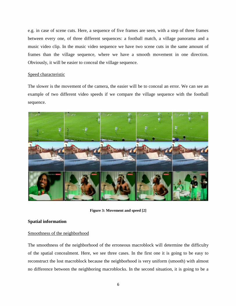
e.g. in case of scene cuts. Here, a sequence of five frames are seen, with a step of three frames
between every one, of three different sequences: a football match, a village panorama and a
music video clip. In the music video sequence we have two scene cuts in the same amount of
frames than the village sequence, where we have a smooth movement in one direction.
Obviously, it will be easier to conceal the village sequence.
Speed characteristic
The slower is the movement of the camera, the easier will be to conceal an error. We can see an
example of two different video speeds if we compare the village sequence with the football
sequence.
Figure 3: Movement and speed [2]
Spatial information
Smoothness of the neighborhood
The smoothness of the neighborhood of the erroneous macroblock will determine the difficulty
of the spatial concealment. Here, we see three cases. In the first one it is going to be easy to
reconstruct the lost macroblock because the neighborhood is very uniform (smooth) with almost
no difference between the neighboring macroblocks. In the second situation, it is going to be a

7
little bit more difficult; we have to look for the edges and then, recover the line. The third case is
an example where the neighbors cannot help us to recover the macroblock because they do not
give any information about the lost part (in this case, the eye).
Figure 4: Smoothness of the neighborhood [2]
Error Characteristics
• Lost information
• Size and form of the lost region
• I/P frame
If the error is situated in the I frame, it is going to affect more critically the sequence because it
will affect all the frames until the next I frame and I frames do not have any other reference but
themselves. If the error is situated in a P frame it will affect the rest of the frames until the next I
frame but we still have the previous I frame as a reference.
Error Concealment Techniques:
The main task of error concealment is to replace missing parts of the video content by previously
decoded parts of the video sequence in order to eliminate or reduce the visual effects of bit
stream error. Error concealment exploits the spatial and temporal correlations between the
neighboring image parts within the same frame or from the past and future frames.

8
The various error concealment methods can be divided into two categories: error concealment
methods in the spatial domain and error concealment methods in the time domain.
Spatial domain error concealment utilizes information from the spatial smoothness nature of the
video image. Each missing pixel of the corrupted image part is interpolated from the intact
surroundings pixels. Weighted averaging is an example of a spatial domain error concealment
method.
Temporal domain error concealment utilizes the temporal smoothness between adjacent frames
within the video sequence. The simplest implementation of this method is replacing the missing
image part with the spatially corresponding part inside a previously decoded frame, which has
maximum correlation with the affected frame. Examples of temporal domain error concealment
methods include the copy-paste algorithm, the boundary matching algorithm and the block
matching algorithm.
Spatial Error Concealment:
All error concealment methods in spatial domain are based on the same idea which says that the
pixel values within the damaged macroblocks can be recovered by a specified combination of the
pixels surrounding the damaged macroblocks. In this technique, the interpixel difference
between adjacent pixels for an image is determined. The interpixel difference is defined as the
average of the absolute difference between a pixel and its four surrounding pixels. This property
is used to perform error concealment.
The first step in implementing spatial based error concealment is to interpolate the pixel values
within the damaged macroblock from four next pixels in its four 1-pixel wide boundaries. This
method is known as ‘weighted averaging’, because the missing pixel values can be recovered by
calculating the average pixel values from the four pixels in the four 1-pixel wide boundaries of
the damaged macroblock weighted by the distance between the missing pixel and the four
macroblocks boundaries (upper, down, left and right).

9
Figure 5: Weighted Averaging algorithm for spatial error concealment [2]
The formula used for weighed averaging is as follows [2]:
(1)
Temporal Error Concealment:
It is easier to conceal linear movements in one direction because pictures can be predicted from
previous frames (the scene is almost the same). If there are movements in many directions or
scene cuts, finding a part of previous frame that is similar is more difficult, or even impossible.

10
Copy paste Algorithm:
It replaces the missing image part with the spatially corresponding part inside a previously
decoded frame, which has maximum correlation with the affected frame.
Figure 6: Copy paste algorithm [1]
Boundary matching:
Let B be the area corresponding to a one pixel wide boundary of a missing block in the nth frame
Fn. Motion vectors of the missing block as well as those of its neighbors are unknown. The
coordinates [ˆx, ˆy] of the best match to B within the search area A in the previous frame Fn−1
have to be found. The equation used is as follows: [1]
(2)
The sum of absolute differences (SAD) is chosen as a similarity metric for its low computational
complexity. The size of B depends on the number of correctly received neighbors M, boundaries
of which are used for matching.

11
Figure 7: Boundary matching algorithm [1]
Block matching:
Better results can be obtained by looking for the best match for the correctly received MB on top,
bottom, left or right side of the missing MB. The equation used is as follows: [1]
(3)
where ‘AD’ represents the search area for the best match of MBD, with its center spatially
corresponding to the start of the missing MB.
The final position of the best match is given by an average over the positions of the best matches
found for the neighboring blocks, computed as follows: [1]
(4)
The MB sized area starting at the position [ˆx, ˆy] in Fn−1 is used to conceal the damaged MB in
Fn. To reduce the necessary number of operations, only parts of the neighboring MBs can be
used for the MV search.

12
Figure 8: Block matching [1]
Quality Metrics:
An objective image quality metric can play a variety of roles in image processing applications.
First, it can be used to dynamically monitor and adjust image quality. For example, a network
digital video server can examine the quality of video being transmitted in order to control and
allocate streaming resources. Second, it can be used to optimize algorithms and parameter
settings of image processing systems. Third, it can be used to benchmark image processing
systems and algorithms. In this project the following quality metrics are used.
i. Peak Signal to Noise Ratio (PSNR)
ii. Distortion Artifacts
iii. Spatial Information (SI) & Temporal Information (TI)
iv. Structural Similarity Index Metric (SSIM)
v. Bjontegaard Distortion – Bit Rate (BD-BR)
vi. Bjontegaard Distortion – PSNR (BD-PSNR)
Peak Signal to Noise ratio (PSNR)
In scientific literature it is common to evaluate the quality of reconstruction of a frame F by
analyzing its peak signal to noise ratio (PSNR). There are different ways of calculating PSNR.
One is frame-by-frame and the other is the overall average.
The Joint Model reference software outputs PSNR for every component c of the YUV color
space for every frame k. The PSNR for an 8 bit PCM (0-255 levels) is calculated using: [1]

13
𝑃𝑆𝑁𝑅𝑘(𝑐)
= 10. 𝑙𝑜𝑔102552
𝑀𝑆𝐸𝑘(𝑐) [𝑑𝐵] (5)
Where, 𝑃𝑆𝑁𝑅𝑘 is the PSNR for the 𝑘𝑡ℎ frame and 𝑀𝑆𝐸𝑘 is the mean square error of the 𝑘𝑡ℎ
frame, given by: [1]
𝑀𝑆𝐸𝑘(𝑐)
=1
𝑀.𝑁∑ ∑ [𝐹(𝑖, 𝑗)𝑀
𝑗=1𝑁𝑖=1 − 𝐹0(𝑖, 𝑗)]
2 (6)
Where, 𝑁 ×𝑀 is the size of the frame, 𝐹0 is the original frame and 𝐹 is the current frame. The
average PSNR is calculated using: [1]
𝑃𝑆𝑁𝑅𝑎𝑣(𝑐)
=1
𝑁𝑓𝑟∑ 𝑃𝑆𝑁𝑅𝑘
(𝑐)𝑁𝑓𝑟
𝑘=1 (7)
Where, 𝑁𝑓𝑟 is the number of frames and 𝑃𝑆𝑁𝑅𝑘 is the PSNR for the 𝑘𝑡ℎ frame.
Distortion Artifacts
Here measurement of distortion artifacts like blockiness and blurring is done. Blockiness is
defined as the distortion of the image characterized by the appearance of an underlying block
encoding structure [1]. This metric compares the power of blurring of two images. If the value of
the metric for first picture is greater, than the value for the second picture, it means that second
picture is more blurred, than first. On the other hand, blurriness is defined as a global distortion
over the entire image, characterized by reduced sharpness of edges and spatial detail [1]. This
metric was created to measure the visual effect of blocking. If the value of the metric for first
picture is greater, than the value for the second picture, it means that first picture has more
blockiness, than the second picture.

14
Figure 9: Blockiness in an image [1]
Figure 10: Blurriness in an image [1]
Spatial and temporal Information
Spatial and temporal information of video sequences play a crucial role in determining the
amount of video compression that is possible, and consequently, the level of impairment that is
suffered when the scene is transmitted over a fixed-rate digital transmission service channel.
Spatial and temporal measures that can be used to classify the type of a sequence are presented in
order to assure appropriate coverage of the spatial-temporal plane in subjective video quality

15
tests. Spatial and temporal information of video sequences tell us the amount of video
compression possible and the level of impairment that is suffered during transmission.
The Spatial Information (SI) is based on the Sobel filter [1]. The Sobel filter generates an
image emphasizing the edges. Each video frame 𝐹𝑛 at time n is first filtered with the Sobel filter
(𝑆𝑜𝑏𝑒𝑙 (𝐹𝑛)). Next, the standard deviation over the pixels (𝑠𝑡𝑑𝑠𝑝𝑎𝑐𝑒) in each Sobel-filtered frame
is computed. This operation is repeated for each frame in the video sequence and results in a time
series of spatial information of the scene. The mean value in the time series (𝑚𝑒𝑎𝑛𝑡𝑖𝑚𝑒) is
chosen to represent the spatial information content of the scene. It can be measured using: [1]
𝑆𝐼 = 𝑚𝑒𝑎𝑛𝑡𝑖𝑚𝑒{𝑠𝑡𝑑𝑠𝑝𝑎𝑐𝑒[𝑆𝑜𝑏𝑒𝑙 (𝐹𝑛)]} (8)
The Temporal Information (TI) is based upon the motion difference feature 𝑀𝑛(i,j), which is the
difference between the pixel values at the same location in space but at successive frames. It can
be measured using: [1]
𝑀𝑛(𝑖, 𝑗) = 𝐹𝑛(𝑖, 𝑗) − 𝐹𝑛−1(𝑖, 𝑗) (9)
where 𝐹𝑛(𝑖, 𝑗) is the pixel at the 𝑖𝑡ℎ row and 𝑗𝑡ℎ column of the 𝑛𝑡ℎ frame in time.
The measure of TI is computed as the mean time (𝑚𝑒𝑎𝑛𝑡𝑖𝑚𝑒) of the standard deviation over
space (𝑠𝑡𝑑𝑠𝑝𝑎𝑐𝑒) of 𝑀𝑛(𝑖, 𝑗) over all i and j: [1]
𝑇𝐼 = 𝑚𝑒𝑎𝑛𝑡𝑖𝑚𝑒{𝑠𝑡𝑑𝑠𝑝𝑎𝑐𝑒[𝑀𝑛(𝑖, 𝑗)]} (10)
More the motion in adjacent frames, higher the values of TI.
Structural Similarity Index Metric (SSIM)
The main function of the human visual system (HVS) is to extract structural information from
the viewing field, and HVS is highly adapted for this purpose. Therefore, a measurement of
structural information loss can provide a good approximation to perceived image distortion.
SSIM compares local patterns of pixel intensities that have been normalized for luminance and
contrast. The luminance of the surface of an object being observed is the product of the
illumination and the reflectance, but the structures of the objects in the scene are independent of

16
the illumination. Consequently, to explore the structural information in an image, the influence
of illumination must be separated.
Figure 11: SSIM measurement [1]
Let x and y be two image patches extracted from the same spatial location of two images being
compared. Let 𝜇𝑥 and 𝜇𝑦 be their means and 𝜎𝑥2 and 𝜎𝑦
2 be their variances. Also, let 𝜎𝑥𝑦2 be the
variance of x and y. The luminance, contrast and structure comparison are given by: [1]
(11)
(12)
(13)
Where 𝐶1, 𝐶2 and 𝐶3 are all constants given by: [1]
(14)

17
L is the dynamic range of the pixel values (L = 255 for 8 bits/pixel gray scale images), and 𝐾1 ≪
1 and 𝐾2 ≪ 1 are scalar constants. The general SSIM can be calculated as follows: [1]
(15)
Where 𝛼, 𝛽 𝑎𝑛𝑑 𝛾 are parameters which define the relative importance of the three components.
Generation of errors
This is done by modifying the function “decode one slice” that is found in the “image.c file” of
the decoder source code. The purpose of this function is, as its name says, decoding one slice.
The operation is quite simple: it takes a slice, reads macroblocks successively from the bitstream
and decodes them by calling the function “decode one macroblock”. When the flag ”end of slice”
gets the value ”TRUE” we go out of the function until the next slice needs to be decoded.
The error is generated in the frames of the video sequence randomly with a uniform distribution.
When a new slice is detected (every time the function “decode one slice” is called), a random
threshold number from 0 to 99 is generated. Then, we compare this value with the error rate per
slice we want to introduce (we took it from the “decoder.cfg” file as a percentage). If the
generated value is lower than the error rate, the whole slice is treated as erroneous. Here, instead
of calling the function “decode one macroblock”, the selected error concealment method will be
used to conceal the slice.
Error input by command line
We have seen that, to introduce an error rate per slice, we have to write the required percentage
in the “decoder.cfg” file from where it is compared with the random threshold generated. The
problem is that C generates random numbers using pseudo-random sequences. There the
sequence of random numbers will always be the same.

18
Figure 12: Akiyo without and with error [1]
Figure 13: Fussball without and with error [1]
19
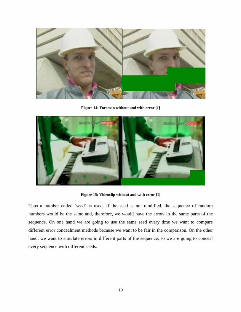
Figure 14: Foreman without and with error [1]
Figure 15: Videoclip without and with error [1]
Thus a number called ‘seed’ is used. If the seed is not modified, the sequence of random
numbers would be the same and, therefore, we would have the errors in the same parts of the
sequence. On one hand we are going to use the same seed every time we want to compare
different error concealment methods because we want to be fair in the comparison. On the other
hand, we want to simulate errors in different parts of the sequence, so we are going to conceal
every sequence with different seeds.

20
Standard way of running the decoder is: [1]
Modified way: [1]

21
References:
[1] I. C. Todoli, “Performance of Error Concealment Methods for Wireless Video,” Ph.D.
thesis, Vienna University of Technology, 2007.
[2] V.S. Kolkeri "Error Concealment Techniques in H.264/AVC, for Video Transmission
over Wireless Networks", M.S. Thesis, Department of Electrical Engineering, University of
Texas at Arlington, Dec. 2009 Online:
http://www.uta.edu/faculty/krrao/dip/Courses/EE5359/index_tem.html.
[3] Y. Chen et al, “An Error Concealment Algorithm for Entire Frame Loss in Video
Transmission,” IEEE, Picture Coding Symposium, Dec. 2004.
[4] H. Ha, C. Yim and Y. Y. Kim, “Packet Loss Resilience using Unequal Forward Error
Correction Assignment for Video Transmission over Communication Networks,” ACM digital
library on Computer Communications, vol. 30, pp. 3676-3689, Dec. 2007.
[5] Y. Xu and Y. Zhou, “H.264 Video Communication Based Refined Error Concealment
Schemes,” IEEE Transactions on Consumer Electronics, vol. 50, issue 4, pp. 1135–1141, Nov.
2004.
[6] M. Wada, “Selective Recovery of Video Packet Loss using Error Concealment,” IEEE
Journal on Selected Areas in Communication, vol. 7, issue 5, pp. 807-814, June 1989.
[7] S. –K. Kwon, A. Tamhankar and K.R. Rao, ”Overview of H.264 / MPEG-4 Part 10”, J.
Visual Communication and Image Representation, vol. 17, pp.186-216, Apr. 2006.
[8] Video Trace research group at ASU, “YUV video sequences,” Online:
http://trace.eas.asu.edu/yuv/index.html.
[9] Z. Wang, “The SSIM index for image quality assessment,” Online:
http://www.cns.nyu.edu/zwang/files/research/ssim/.
[10] H.264/AVC Reference Software Download: Online:
http://iphome.hhi.de/suehring/tml/download/
[11] S. K. Bandyopadhyay et al, “An error concealment scheme for entire frame losses for
H.264/AVC”, IEEE Sarnoff Symposium, pp. 1-4, Mar. 2006.
[12] MSU video quality measurement tool: Online:
http://compression.ru/video/quality_measure/video_measurement_tool_en.html.
[13] G. Bjontegaard, “Calculation of average PSNR differences between RD-Curves”, ITU-T
SG16, Doc. VCEG-M33, 13th VCEG meeting, Apr. 2001. Online: http://wfpt3.itu.int/av-
arch/video-site/0104_Aus/VCEG-M33.doc.

22
[14] D. Grois, B. Bross and D. Marpe, “HEVC/H.265 Video Coding Standard (Version 2)
including the Range Extensions, Scalable Extensions, and Multiview Extensions,” (Tutorial),
IEEE ICIP, Quebec City, Canada, Sept. 2015. Online:
https://datacloud.hhi.fraunhofer.de/owncloud/public.php?service=files&t=8edc97d26d46d4458a
9c1a17964bf881. Password: a2FazmgNK.