ERROR ASSESSMENT FOR EMERGING TRAFFIC DATA...

ERROR ASSESSMENT FOR EMERGING TRAFFIC

DATA COLLECTION DEVICES

FINAL PROJECT REPORT

by

Yinhai Wang,

Ed McCormack, Bahar Namaki Araghi,

Yegor Malinovskiy, Jonathan Corey,

and Tianxing Cheng

for

Pacific Northwest Transportation Consortium (PacTrans)

USDOT University Transportation Center for Federal Region 10

University of Washington

More Hall 112, Box 352700

Seattle, WA 98195-2700

i

Disclaimer

The contents of this report reflect the views of the authors, who are responsible for the

facts and the accuracy of the information presented herein. This document is disseminated

under the sponsorship of the U.S. Department of Transportation’s University

Transportation Centers Program, in the interest of information exchange. The Pacific

Northwest Transportation Consortium and the U.S. Government assumes no liability for

the contents or use thereof.

ii

Technical Report Documentation Page

1. Report No. 2. Government Accession No. 3. Recipient’s Catalog No.

4. Title and Subtitle 5. Report Date Error Assessment for Emerging Traffic Data Collection Devices

September 15, 2014

6. Performing Organization Code

7. Author(s) 8. Performing Organization Report No. Dr. Yinhai Wang, Bahar Namaki Araghi, Jonathan Corey, Yegor Malinovskiy, Tianxing

Cheng

18-624909

9. Performing Organization Name and Address 10. Work Unit No. (TRAIS) PacTrans

Pacific Northwest Transportation Consortium, University Transportation

Center for Region 10

University of Washington More Hall 112 Seattle, WA 98195-2700

Univeristy of Washington Smart

Transportation Applications and Research Laboratory

University of Washington More Hall 201

Seattle, WA 98195

11. Contract or Grant No.

DTRT12-UTC10

12. Sponsoring Organization Name and Address 13. Type of Report and Period Covered United States of America

Department of Transportation

Research and Innovative Technology Administration

Research 9/1/2012-7/31/2014

14. Sponsoring Agency Code

15. Supplementary Notes Report uploaded at www.pacTrans.org

16. Abstract Providing accurate and reliable travel time information to roadway users is a critical part of Advanced Traffic Management Systems (ATMS) and

Advanced Travelers Information Systems (ATIS). Access to travel time information can significantly influence the decision making on both the supply

side (i.e. efficient management of network capacity, saving travel time, reducing congestion etc.) and the demand side (i.e. mode choice, route choice etc.) of transportation. In this context, the need for accurate and reliable travel time information sources is becoming increasingly apparent.

Identifying the sensors best suited to providing travel time data for a given corridor is an important step in the process of providing travel time

data. Currently, there are very few studies available that evaluate the effectiveness of various travel time data collection technologies side-by-side, thus it is often unclear which approach should be used for a given application. Therefore, a comprehensive overview of existing technologies as well as a side-

by-side evaluation will provide more insight into selecting the appropriate technology for a given application. This evaluation is intended to provide

decision support for transportation agencies selecting travel time systems based on the accuracy, reliability and cost of each system.

Ultimately, each system in the analysis has different strengths and weaknesses that should be considered in addition to their accuracy and sample

rates. Some systems can provide additional data; others trade accuracy and coverage for cost or portability. Ultimately, engineers will need to weigh their

requirements for accuracy and sample rates against the other engineering constraints imposed on their system. For example, the BlueTOAD units installed on SR 522 and I-90 are solar powered and use cellular data networks, reducing infrastructure and deployment costs. The BlipTrack units have

higher sampling rates and marginal accuracy superiority in exchange for power requirements. The Inrix data does not require any DOT infrastructure and

has wide availability. ALPR units have high accuracy and a comparatively high installation cost. The Sensys system has perhaps the most complicated set of tradeoffs. Sensys magnetometers can be used as replacements for loop detectors in intersection operations, making the marginal costs of adding

Sensys re-identification lower at some intersections than others.

17. Key Words 18. Distribution Statement Travel Time Estimation, Error Matrix, Reliability, Traffic Volume and Speed No restrictions.

19. Security Classification (of this

report)

20. Security Classification (of this

page)

21. No. of Pages 22. Price

Unclassified. Unclassified. NA

Form DOT F 1700.7 (8-72) Reproduction of completed page authorized

http://www.pactrans.org/

grad_assist

Typewritten Text

grad_assist

Typewritten Text

2012-S-UW-0018 01538108

iii

Table of Contents

Table of Contents ......................................................................................................................... iii

List of Figures ................................................................................................................................. v

List of Tables ............................................................................................................................... viii

Glossary .......................................................................................................................................... ix

Executive Summary ....................................................................................................................... x

Chapter 1 Introduction ............................................................................................................ 1

1.1 Background .............................................................................................................. 1

Chapter 2 Travel Time Data Collection Methodology .......................................................... 5

2.1 Probe Vehicle Method .............................................................................................. 5

2.1.1 ITS Probe Vehicle Data Collection Systems ................................................ 5

2.1.2 General Advantages and Disadvantages ...................................................... 6

2.2 Vehicle Re-identification Method ............................................................................ 7

2.2.1 Vehicle Re-identification Data Collection Systems ..................................... 7

2.2.2 General Advantages and Disadvantages ...................................................... 8

2.3 Point Based Volume and Speed Estimation Method ............................................... 9

2.3.1 Point Based Volume and Speed Estimation Data Collection Systems ........ 9

2.3.2 General Advantages and Disadvantages .................................................... 10

Chapter 3 Experiment Design and Data Collection ............................................................ 13

3.1 State Route 522 in Seattle, Washington ................................................................. 13

3.1.1 Data availability on SR 522 ....................................................................... 14

3.2 I-90 Freeway Test At Snoqualmie Pass, Washington ............................................ 18

3.2.1 Data availability on I-90 ............................................................................. 19

3.3 Traffic Data Collection Techniques ....................................................................... 21

3.3.1 Volume and Speed Estimation Technologies ............................................. 21

3.3.2 Vehicle Re-identification Technologies ..................................................... 26

3.3.3 3rd Party Inrix Data .................................................................................... 36

Chapter 4 Evaluation Frame Work ...................................................................................... 38

4.1 Error and Reliability Matrix ................................................................................... 38

4.1.1 Data Distribution ........................................................................................ 38

iv

4.1.2 Travel Time Accuracy and Error ............................................................... 39

4.1.3 Data Analysis Resolutions ......................................................................... 40

4.2 Data Availability .................................................................................................... 41

4.2.1 Types of Data ............................................................................................. 46

4.3 Data analysis and discussions for SR 522 .............................................................. 47

4.3.1 Sample Count ............................................................................................. 47

4.4 Travel Time ............................................................................................................ 62

4.4.1 Westbound Travel Time ............................................................................. 62

4.4.2 Eastbound Travel Time .............................................................................. 75

4.5 Data Analysisfor I-90 ............................................................................................. 81

4.6 Data Manipulation and Sensor Evaluation Conclusions ........................................ 89

Chapter 5 Summary of the results and discussions ............................................................. 94

References ..................................................................................................................................... 98

Appendix A: SR 522 and I-90 Corridor Details ...................................................................... 103

Appendix B: Architecture of Sensys Technology .................................................................... 106

v

List of Figures

Figure 1.1 Benefit-Accuracy relationship for case study in Los Angeles (Source: Toppen and

Wunderlich, 2003) ............................................................................................................................ 3

Figure 3.1 Sensor locations and segments along the SR 522 corridor ........................................... 15

Figure 3.2 Sensor locations and segments along the I-90 Snoqualmie Pass corridor .................... 19

Figure 3.3 EDI Oracle 2E series Inductive Loop Detector ............................................................ 22

Figure 3.4 Loop Detector System Architecture ............................................................................. 23

Figure 3.5 Reno A&E Model C-1100 Series Inductive Loop Detectors ....................................... 24

Figure 3.6 Traficon VIP3D.2 sensor .............................................................................................. 25

Figure 3.7 VDPU System Architecture .......................................................................................... 26

Figure 3.8 Pips P327 Spike ALPR sensor ...................................................................................... 28

Figure 3.9 BlueTOAD sensor design and components .................................................................. 30

Figure 3.10 BlipTrack sensor design and components .................................................................. 31

Figure 3.11 BlipTrack WiFi sensor design and components ......................................................... 32

Figure 3.12 Architecture of BlipTrack solution ............................................................................. 33

Figure 3.13 Sensys wireless vehicle detection system ................................................................... 35

Figure 4.1 Capture rate comparison on westbound SR 522 between April 5th, 2013 through June

8th 2013 .......................................................................................................................................... 50

Figure 4.2 Comparing capture rate of different systems from 83rd Pl. NE to 68th Ave. NE (WB)

for May 1st, 2013 through May 8

th, 2013 ....................................................................................... 51

Figure 4.3 Comparing capture rate of different systems from 68th Ave. NE to SR 104 (WB) for

May 1st, 2013 through May 8th, 2013 ........................................................................................... 52

Figure 4.4 Comparing capture rate of different systems from SR 104 to NE 153rd St. (WB) for

May 1st, 2013 through May 8th, 2013 ........................................................................................... 53

Figure 4.5 Westbound Volume and Capture Rates for Wednesday May 1, 2013 from 83rd Place

NE to 68th Avenue NE ................................................................................................................... 55

Figure 4.6 Westbound Volume and Capture Rates for Wednesday May 1, 2013 From 68th

Avenue to SR-104 Junction ............................................................................................................ 56

Figure 4.7 Westbound Volume and Capture Rates for Wednesday May 1, 2013 From SR-104

Junction to NE 153rd Street .......................................................................................................... 57

vi

Figure 4.8 Comparing capture rate of different systems from 68th Ave. NE to 83rd Pl. NE (EB)

for May 1st, 2013 through May 8

th, 2013 ....................................................................................... 59

Figure 4.9 Comparing capture rate of different systems from SR 104 to 68th Ave. NE (EB) for

May 1st, 2013 through May 8

th, 2013 ............................................................................................. 60

Figure 4.10 Comparing capture rate of different systems from NE 153rd St. to SR 104 (EB) for

May 1st, 2013 through May 8

th, 2013 ............................................................................................. 61

Figure 4.11 Travel time plot for 83rd

Pl. NE to 68th

Ave. NE (WB) for May 1st, 2013 through May

8th

, 2013 .......................................................................................................................................... 63

Figure 4.12 Travel time plot for 68th

Ave. NE to SR 104 (WB) for May 1st, 2013 through May 8

th,

2013 ................................................................................................................................................ 64

Figure 4.13 Travel time plot from SR 104 to NE 153rd St. (WB) for May 1st, 2013 through May

8th, 2013 ......................................................................................................................................... 65

Figure 4.14 The MAPE variation for 83rd Pl. NE to 68th Ave. NE (WB) over 24 hours on

Wednesdays over the period of April 5th

, 2013 through June 8th

, 2013 ......................................... 67

Figure 4.15 The MAPE variation from68th Ave. NE to SR 104 (WB) over 24 hours on



, 2013 ......................................... 68

Figure 4.16 The MAPE variation from SR 104 to NE 153rd St. (WB) over 24 hours on



, 2013 ......................................... 69

Figure 4.17 Travel time plot from 68th Ave. NE to 83rd Pl. NE (EB) for May 1st, 2013 through

May 8th, 2013 ................................................................................................................................ 76

Figure 4.18 Travel time plot from SR 104 to 68th Ave. NE (EB) for May 1st, 2013 through May

8th , 2013 ........................................................................................................................................ 77

Figure 4.19 Travel time plot from NE 153rd St. to SR 104 (EB) for May 1st, 2013 through May

8th, 2013 ......................................................................................................................................... 78

Figure 4.20 Travel times on I-90 from Ellensburg (MP 109) to Easton (MP 70) for May 1st, 2013

through May 8th

, 2013 .................................................................................................................... 83

Figure 4.21 Travel times on I-90 from Easton (MP 70) to the Snoqualmie Pass (MP 52) for May

1st, 2013 through May 8

th, 2013 ..................................................................................................... 84

Figure 4.22 Travel times on I-90 from the summit (MP 52) to North Bend (MP 32) for May 1st,

2013 through May 8th

, 2013 ........................................................................................................... 85

Figure 4.23 May 2nd

closure of I-90 and sensor response .............................................................. 86

vii

Figure 4.24 May 15th

closure of I-90 and sensor responses ........................................................... 87

Figure 4.25 I-90 data analysis interface for sensors.uwdrive.net ................................................... 92

Figure 4.26 SR 522 data analysis interface for sensors.uwdrive.net .............................................. 92

viii

List of Tables

Table 3.1 List of technologies implemented along SR 522 ........................................................... 16

Table 3.2 List of sensors mounted at SR 522 intersections ........................................................... 17

Table 3.3 List of technologies implemented on I-90 ..................................................................... 20

Table 3.4 List of sensors mounted on I-90 ..................................................................................... 20

Table 4.1 Data Availability on SR-522 Westbound ....................................................................... 43

Table 4.2 Data Availability on SR-522 Eastbound ........................................................................ 44

Table 4.3 Data availability by month and system for I-90 ............................................................. 45

Table 4.4 Data availability and type of analysis on westbound and eastbound SR 522 ................ 46

Table 4.5 Data availability and type of analysis on westbound and eastbound I-90 ..................... 47

Table 4.6 Sample counts on westbound SR 522 during April 5th


2013 .... 49

Table 4.7 Sample counts on eastbound SR 522 over period of April 5th


,

2013 ................................................................................................................................................ 58

Table 4.8 Hourly descriptive statistics for westbound over the period of April 5th

, 2013 through

June 8th

, 2013 ................................................................................................................................. 71

Table 4.9 Results of the MAPE for hourly analysis over the period of April 5th

, 2013 through

June 8th

, 2013 ................................................................................................................................. 72

Table 4.10 Travel time accuracy analysis for westbound SR 522 for the period of April 5th

, 2013

through June 8th

, 2013 .................................................................................................................... 74

Table 4.11 Hourly descriptive statistics for eastbound SR 522 over the period of April 5th

, 2013

through June 8th

, 2013 .................................................................................................................... 80

ix

Glossary

ALPR Automated License Plate Reader

ANPR Automated Number Plate Reader

APVD Aggregated Probe Vehicle Data

ATIS Advanced Travelers Information Systems

ATMS Advanced Traffic Management Systems

AVI Automatic Vehicle Identification

AVL Automatic Vehicle Location

CCD Charge-Coupled Devices

CFD Cumulative Frequency Distributions

DRG Dynamic Route Guidance

EDI Eberle Design Inc

FHWA Federal Highway Administration

ITS Intelligent Transportation Systems

GPS Global Positioning System

LAN Local Area Network

LCD Liquid-Crystal Display

LED Light-Emitting-Diode

MAC Media Access Control

MAD Mean Absolute Deviation

MAPE Mean Absolute Percent Error

MPE Mean Percent Error

PC Personal Computer

PDA Personal Digital Assistant

RMSE Root Mean Squared Error

SDPE Standard Deviation Of Percentage Error

SR State Route

TCI TrafficCast International

VDPU Video Detection Processor Unit

VIL Virtual Induction Loop

VIP Video Image Processor

x

Executive Summary

Providing accurate and reliable travel time information to roadway users is a critical part

of Advanced Traffic Management Systems (ATMS) and Advanced Travelers Information

Systems (ATIS). Access to travel time information can significantly influence the decision

making on both the supply side (i.e. efficient management of network capacity, saving travel

time, reducing congestion etc.) and the demand side (i.e. mode choice, route choice etc.) of

transportation. In this context, the need for accurate and reliable travel time information sources

is becoming increasingly apparent.

Identifying the sensors best suited to providing travel time data for a given corridor is an

important step in the process of providing travel time data. Currently, there are very few studies

available that evaluate the effectiveness of various travel time data collection technologies side-

by-side, thus it is often unclear which approach should be used for a given application. Therefore,

a comprehensive overview of existing technologies as well as a side-by-side evaluation will

provide more insight into selecting the appropriate technology for a given application. This

evaluation is intended to provide decision support for transportation agencies selecting travel

time systems based on the accuracy, reliability and cost of each system.

The choice of a sensor system and its corresponding accuracy could play a significant role

on the benefits of the information provided for the users (i.e. utility) according to a FHWA report

by Toppen and Wunderlich (2003). The relationship between accuracy of the information

obtained by ATIS and the benefits for the users was determined for a case study in Los Angeles

(seeFigure 1.1). The researchers found that when accuracy drops below a critical point, users are

better off not using the data provided by the ATIS and relying instead on experience with

historical traffic patterns.

A good approach to judging sensor accuracy is to look at the MAD to judge the expected

magnitude of error. Then examine the MPE to determine whether there are systematic biases to

the data. Note that for travel time it is reasonable to expect errors to be skewed toward longer

xi

travel times in most cases, since travel time underestimation is bounded on the lower end by zero.

This is particularly true for SR 522 where individual segment free flow travel times are on the

order of a minute and the whole corridor can be traversed in five minutes. The MAPE is useful to

find the relative magnitude of the error. Finally, the RMSE is useful in determining whether a

few large errors or many smaller errors are occurring. Between the four measures of error, a user

can determine the magnitude of error, its biases, the relative impact of that error and the

magnitude of the typical error.

This study focuses on two test corridors. The first test corridor is SR 522 between the NE

153rd

Street and 83rd

Place NE intersections. This section of SR 522 is an urban arterial with

frequent intersections. This corridor experiences heavy daily commuting traffic and has frequent

incidents that can make travel times unpredictable. An automated license plate reader system has

been in place on the SR 522 corridor for a number of years with three westbound segments in the

study area, from 83rd

Pl. NE to 68th

Ave. NE, 68th

Ave. NE to SR 104 and SR 104 to NE 153rd

St.

For this analysis, even though the ALPR system has different segments on eastbound SR 522, the

analysis used the same segments for eastbound because every other system used the same

segments eastbound and westbound.

The second test corridor is on I-90 from milepost 109 (Ellensburg, WA) to milepost 32

(North Bend, WA). This section of I-90 is a rural freeway from western Washington to eastern

Washington over the Snoqualmie Pass whose summit is at milepost 52. There were no pre-

existing travel time measurement systems on I-90 before this study. Segments on I-90 are

described by mileposts 32, 52, 70 and 109.

The sensor systems deployed on SR 522 include the pre-existing ALPR system, a Sensys

emplacement on westbound SR 522, the TrafficCast BlueTOAD system, Blip Systems BlipTrack

sensors and a 3rd

party feed from Inrix. The I-90 corridor was instrumented with the BlueTOAD

system in addition to using the Inrix data feed. The ALPR system reads the license plates of

vehicles passing the sensors and holds the license plate number in memory until the vehicle

passes the next sensor location. The Bluetooth and WiFi sensors built into the BlueTOAD and

BlipTrack systems function similarly by reading the MAC address of wireless electronic devices

xii

from location to location. The Sensys system reads the magnetic signature of passing vehicles

and attempts to match vehicles based on signature and platoon organization. The Inrix data is

based on cellphone and GPS data from its users.

Collecting the data for this project has been a significant expenditure of effort. Collecting

data from the Washington State Department of Transportation (WSDOT), Inrix, Sensys,

TrafficCast, and Blip Systems has required the research team to visit multiple websites and

databases. Collating and organizing data with different temporal resolutions, included data and

segments required the research team to find common intervals and expend significant effort just

to make the different data sets comparable.

There are two important factors to consider in analyzing the sensor results. The first is the

accuracy of the reported travel time. To address this, each sensors’ data is compared against the

ALPR system on westbound SR 522. The ALPR system has been previously evaluated and

deemed accurate enough to serve as the ground truth for this study. The lack of ALPR data or

other similarly dependable travel time data source limits the research team’s ability to analyze

eastbound SR 522 and the I-90 corridor. A number of accuracy measures have chosen for this

analysis to give readers more insight into the frequency, severity and directionality of errors.

The westbound SR 522 analysis found that the accuracy of the systems varied by segment with

every system reporting their least accurate travel times on the 83rd

Pl. NE to 68th

Ave.NE

segment. The daily analysis revealed that the systems experienced error spikes during the

morning peak period on all segments. With the exception of the Inrix data, all systems generally

reported satisfactory results, with the Bluetooth and WiFi based systems staying below the 25%

error threshold except during overnight hours and some spikes in the peak periods. It should be

noted that the Sensys travel time used was the 90th

percentile travel time, where the other systems

reported mean or median values, yet still the Sensys system posted acceptable accuracy in most

cases. The Sensys travel time error may be reduced by selecting another one of the ten provided

travel time values.

The systems did have some notable accuracy limitations. Specifically, the BlueTOAD

system can be less reliable overnight when sampling is low. The Inrix system was generally the

xiii

least responsive to traffic changes and tended to have systematically high or low travel times,

probably the results of conservative free flow travel time estimation.

The I-90 and eastbound SR 522 analysis of travel time focused on more qualitative

aspects of system performance. For I-90, the research team was looking for reasonable travel

times and daily traffic patterns as well as response to known road closure events. The eastbound

SR 522 results met expectations based on the westbound analysis, with most patterns repeating,

including the systematic over or underestimation of travel time by Inrix. The I-90 analysis noted

that both systems were able to respond to daily patterns; however, Inrix and BlueTOAD reported

significantly different results on some segments. When the road closure time periods were

examined, both systems had their flaws. The BlueTOAD system continued to report a travel time

for 30 minutes after the road closure and the Inrix data either failed to react significantly to the

closure or reported impossible travel times. Both systems include specific data that can be used to

identify when such event occur.

The collection of sensors assembled for this study is impressive. By setting up so many

sensors on the same corridor and having reliable ground truth data in the form of an established

ALPR system, the WSDOT has made it possible to perform an in-depth analysis of the different

systems. This work shows that sensors of different types and complexities can accomplish the

goal of measuring travel time.

Ultimately, each system in the analysis has different strengths and weaknesses that should

be considered in addition to their accuracy and sample rates. Some systems can provide

additional data; others trade accuracy and coverage for cost or portability. Ultimately, engineers

will need to weigh their requirements for accuracy and sample rates against the other engineering

constraints imposed on their system. For example, the BlueTOAD units installed on SR 522 and

I-90 are solar powered and use cellular data networks, reducing infrastructure and deployment

costs. The BlipTrack units have higher sampling rates and marginal accuracy superiority in

exchange for power requirements. The Inrix data does not require any DOT infrastructure and has

wide availability. ALPR units have high accuracy and a comparatively high installation cost. The

Sensys system has perhaps the most complicated set of tradeoffs. Sensys magnetometers can be

xiv

used as replacements for loop detectors in intersection operations, making the marginal costs of

adding Sensys re-identification lower at some intersections than others.

Note that high level conclusions are presented here. For detailed observations see the

relevant chapters. Readers are specifically encouraged to review Figure 1.1, Figure 4.1, Figure

4.9, Figure 4.10 and Figure 4.24.

1

Chapter 1 Introduction

1.1 Background

Providing accurate and reliable travel time information plays a critical role in Advanced

Traffic Management Systems (ATMS) and also Advanced Travelers Information Systems

(ATIS). Access to travel time information can significantly influence the decision making on

both the supply side (i.e. efficient management of network capacity, saving travel time, reducing

congestion etc.) and the demand side (i.e. mode choice, route choice etc.) of transportation. In

this context, the need for accurate and reliable travel time information sources is becoming

increasingly apparent.

A wide range of travel time data collection technologies have been introduced over the

last decade. While increased focus has been granted to the technological advances in collecting

travel time information, it remains critical to monitor and identify technologies that present the

lowest life cycle cost for obtaining reliable and accurate volume and speed information.

There are very few studies available that evaluate the effectiveness of various travel time

data collection technologies side-by-side, thus it is often unclear which approach should be used

for a given application. Therefore, a comprehensive overview of existing technologies as well as

a side-by-side evaluation will provide more insight into selecting the appropriate technology for a

given application. This evaluation is intended to provide decision support for transportation

agencies selecting travel time systems based on the accuracy, reliability and cost of each system.

The choice of a system and its corresponding accuracy could play a significant role on the

benefits of the information provided for the users (i.e. utility) according to a FHWA report by

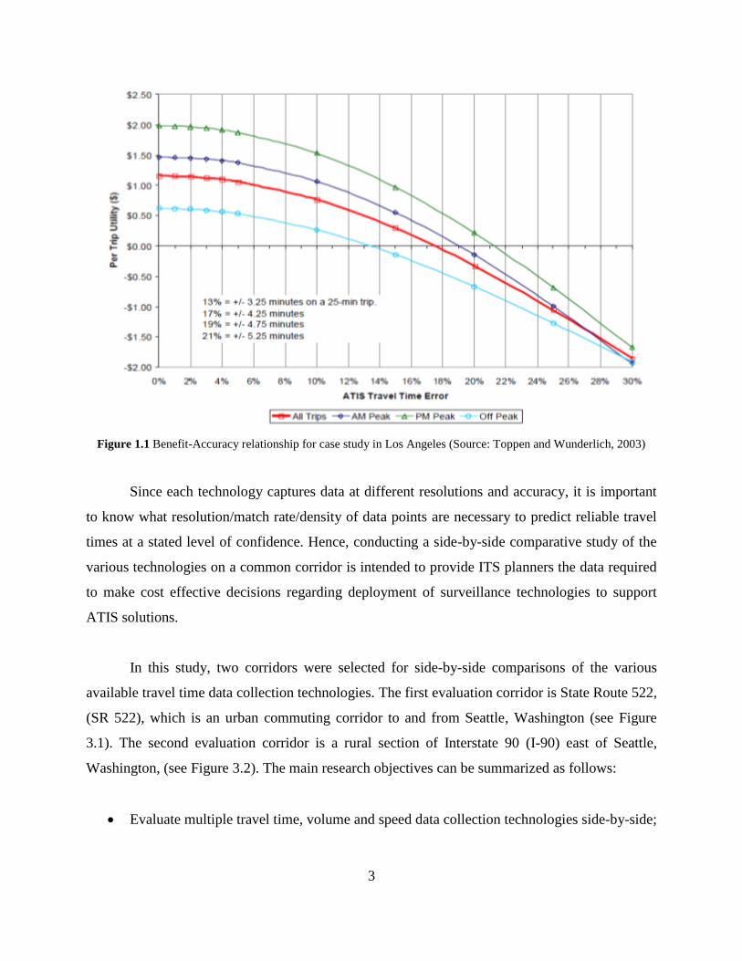
Toppen and Wunderlich (2003). The relationship between accuracy of the information obtained

by ATIS and the benefits for the users was determined for a case study in Los Angeles (see

Figure 1.1). The researchers found that when accuracy drops below a critical point, users are

better off not using the data provided by the ATIS and relying instead on experience with

historical traffic patterns. In Figure 1.1, there are four utility curves representing the utility

2

realized during morning peak trips, evening peak trips, off peak and all trips. For evening peak

trips, represented by the green line on top, the per trip utility realized on 25 minute trip for perfect

and near perfect data was two dollars.

The point at which the ATIS data became worthless to users was at approximately 21%

accuracy, where using the ATIS data produce negative utility values. Beyond a certain point,

below 5% error for example, it makes little sense to invest in improving accuracy as users realize

little to no increased benefit. In this case, funds for ATIS improvements would be better spent in

areas besides improving accuracy, such as expanding coverage to other roadways (Toppen and

Wunderlich, 2003). Therefore, a trade-off needs to be made based on the required accuracy and

the costs of implementing ATIS technologies. Figure 1.1 shows that as travel time error

approaches 20% users realize no value from ATIS data. Innamaa (2009) stated that the net

benefit from an advanced traveler information service was positive in earlier studies only if the

error in service reporting was below the range of 10–25%, but the cost-efficiency of the service

was likely to suffer if error levels below 5% were being pursued. In this study, based on earlier

studies by Innamma (2009), Toppen and Wunderlich (2003), and Jung et al. (2003) the ATIS

error band is defined as 10-25%. Acceptable error is defined as 25% error for this research.

3

Figure 1.1 Benefit-Accuracy relationship for case study in Los Angeles (Source: Toppen and Wunderlich, 2003)

Since each technology captures data at different resolutions and accuracy, it is important

to know what resolution/match rate/density of data points are necessary to predict reliable travel

times at a stated level of confidence. Hence, conducting a side-by-side comparative study of the

various technologies on a common corridor is intended to provide ITS planners the data required

to make cost effective decisions regarding deployment of surveillance technologies to support

ATIS solutions.

In this study, two corridors were selected for side-by-side comparisons of the various

available travel time data collection technologies. The first evaluation corridor is State Route 522,

(SR 522), which is an urban commuting corridor to and from Seattle, Washington (see Figure

3.1). The second evaluation corridor is a rural section of Interstate 90 (I-90) east of Seattle,

Washington, (see Figure 3.2). The main research objectives can be summarized as follows:

Evaluate multiple travel time, volume and speed data collection technologies side-by-side;

4

Determine the relative accuracy and performance (Error Matrix) of the evaluated

technologies;

Determine the relative reliability (Reliability Matrix) of the evaluated technologies.

Define appropriate technologies for common data collection scenarios and needs.

5

Chapter 2 Travel Time Data Collection Methodology

Several data collection techniques can be used to measure or collect travel time. Many of

the technologies being evaluated in this study use different methodologies to generate travel time

information. These various techniques can be classified into a few generalized methodologies,

such as those using: probe vehicles, vehicle re-identification, and volume and speed estimation

methods (also referred to as flow estimation techniques). Note that the flow estimation technique

is presented for completeness. These techniques are designed to collect travel times and average

speeds on designated roadway segments or links. A general overview of the various techniques is

provided in the following paragraphs.

2.1 Probe Vehicle Method

The probe vehicle method utilizes instrumented vehicles in the traffic stream and remote

sensing devices to collect travel times (Travel Time Data Collection Handbook, 1998). An ITS

probe vehicle can be a personal, public transit, or commercial vehicle. Generally, methods of

travel time estimation via probe vehicles currently in use rely on GPS systems to gather data

regarding position and speed. These GPS systems may be integrated into the vehicle, such as for

fleet vehicle operations or portable systems such as smart phones. Other systems in use include

transponder and radio-based systems. The goal of the probe vehicle based methodologies is to

estimate travel times for all vehicles in the traffic stream based upon high quality travel time data

from a subset of vehicles in traffic.

2.1.1 ITS Probe Vehicle Data Collection Systems

Probe vehicles may be equipped with several different types of electronic transponders or

receivers, from passive transponders to live GPS transmissions.

Signpost-Based Automatic Vehicle Location (AVL) 2.1.1.1

This technique has mostly been used by transit agencies. With an AVL system, probe

vehicles communicate at intervals with a transmitter and receiver infrastructure. Note that these

systems may be active, with vehicles frequently broadcasting data, or passive, where

6

transponders only broadcast when queried by the transmitter infrastructure. Depending on the

frequency and quality of data transmitted, AVL systems may operate like probe vehicles, or more

as a vehicle re-identification system, discussed later.

Radio Navigation 2.1.1.2

Radio navigation systems use triangulation techniques to locate radio transponders on

vehicles, and are used in route guidance and communication systems. Data are collected by

communication between probe vehicles and a radio tower infrastructure (Mathew, 2013).

Typically, this type of system is used for fleet dispatch, such as for transit, commercial or

government vehicle dispatch.

GPS Position and Speed 2.1.1.3

GPS based systems are increasingly found at the personal level with dedicated GPS

navigation systems and smart phones being the most common implementations. Some of these

systems broadcast data back to service providers for use in providing real-time traffic data.

2.1.2 General Advantages and Disadvantages

The advantages and disadvantages of this method can be summarized as (Travel Time

Data Collection Handbook, 1998):

Advantages

Low cost per unit of data

Continuous data collection

Automated data collection

Data are in electronic format

No disruption of traffic

Disadvantages

High implementation cost (depending on system used)

Fixed infrastructure constraints - Coverage area, including locations of antenna

7

Requires skilled software

Not recommended for small scale data collection efforts

2.2 Vehicle Re-identification Method

Re-identification relies on recording unique characteristics (i.e. a signature) of the target

vehicle to be used to identify the target vehicle at subsequent sensor locations. Vehicle re-

identification is the process collecting vehicle identification data (i.e. signature) and the

timestamp of vehicles passing a road side reader device and matching against data from another

reader passed by the target vehicle to determine the travel time between reader locations.

2.2.1 Vehicle Re-identification Data Collection Systems

Probe vehicles may be equipped with several different types of electronic transponders or

receivers.

Vehicle Signature Matching 2.2.1.1

Estimates travel time by matching (or correlating) unique vehicle signatures between

sequential observation points. These methods can utilize a number of point detectors. Travel time

is then the differences in the times that each (matched) vehicle arrives at the upstream and

downstream sensor stations. One characteristic of signature matching systems is a time delay

built into data collection related to the time it takes for vehicles to travel from one detector to the

next.

Examples of signature matching include license plate readers, inductive loop detector

signature re-identification, magnetometer signature re-identification and Bluetooth/WiFi Media

Access Control address (MAC) re-identification. The unique signature differentiating vehicles in

each case is different, but the methodology is the same. As previously discussed, transponder

based systems with low frequency data collection may operate more like signature based re-

identification systems than probe vehicle based systems.

8

Platoon Matching 2.2.1.2

Platoon matching is a special case of vehicle re-identification that relies on the fact that

vehicles tend to travel in platoons. This method estimates average travel time by matching unique

features of vehicle platoons such as the position and/or distribution of vehicle gaps or unique

vehicles. Platoon matching assumes that vehicles in a platoon will travel at approximately the

same speed and retain approximately the same order between sensor locations. Because of these

assumptions, platoon matching generally requires closely spaced detection points to prevent

platoons from changing too drastically for the algorithms to re-identify between sensors.


The advantages and disadvantages of this method can be summarized as (Travel Time Data

Collection Handbook, 1998):

Advantages

Travel times from a large sample of motorists

Simple Technique

Automated data collection

Data are in electronic format

Provides a continuum of travel times during the data collection period

No disruption of traffic

Disadvantages

Travel time data limited to locations where readers can be positioned;

Limited geographic coverage

Requires skilled software

Inherent personal privacy risk

9

2.3 Point Based Volume and Speed Estimation Method

Volume and speed estimation technologies rely on the classical steady-state traffic flow

relationship between the traffic stream flow rate (q), the traffic stream density (k), and the traffic

stream space-mean-speed ( ) derived by Lighthill and Witham (1955) as follows:

(2.1)

Traffic stream speeds are typically measured in the field using a variety of spot speed

measurement technologies. These approaches try to extrapolate local point data into corridor

level information. The average traffic stream speed can be computed in two different ways: a

time-mean speed and a space-mean speed. The difference in speed computations is attributed to

inherent difference in definitions of time-mean speed and a space-mean speed. The space-mean

speed reflects the average speed over a spatial section of roadway, while the time-mean speed

reflects the average speed of the traffic stream passing a specific stationary point (Rakha and

Zhang, 2005).

2.3.1 Point Based Volume and Speed Estimation Data Collection Systems

Inductive Loop Detectors (ILD) 2.3.1.1

The most common of these spot speed measurement technologies is an inductive loop

detector set to report presence or occupancy (the percentage of time an ILD detects the presence

of a vehicle). The loop coil of an ILD is embedded in a roadway, generally in a square or circle

that generates a magnetic field. When a vehicle enters the detection zone, the sensor is activated

and remains activated until the vehicle leaves detection zone. ILDs can thus identify the presence

and passage of vehicles over a short segment of roadway (typically 5 to 20 meters long) (Rakha

and Zhang, 2005). These surveillance detectors measure the traffic stream flow rate (number of

actuations per unit time), traffic stream speed (in the case of dual loop detectors), and percentage

of time that the detector is occupied. The traditional practice for estimating speeds from single

loop detectors is based on the assumption of a constant average effective vehicle length and

constant speed.

10

Video Detection 2.3.1.2

Video detection systems works based on virtual loop detectors (VIL). AVIL is a virtual

detector created by processing the input of another sensor type into that of a standard induction

loop. VILs are designed to play the same role as a legacy ILD to interface with existing

equipment. In this way, a VIL service gathers real time information of the vehicles traversing this

virtual detector (Gramaglia et. al, 2013). In general, VILs try to mimic the data obtained by

inductive loops and collect the data about vehicle passage, presence, count, and occupancy.

Because of this close emulation VILs share many of the same strengths and weaknesses of

traditional ILDs.

Magnetometers 2.3.1.3

This method relies on matching vehicle signatures from wireless sensors. The sensors

provide a noisy magnetic signature of a vehicle and the precise time when it crosses the sensors.

A match (re-identification) of signatures at two locations gives the corresponding travel time of

the vehicle.


Advantages

Travel times from a large sample of motorists

Simple technique

Provides a continuum of travel times during the data collection period

Performs well in both high and low volume traffic and in different weather conditions

(Sreedevi, 2005).

Disadvantages

Expensive deployment and maintenance costs (Particularly for invasive ILDs)

Trouble measuring low-speed vehicles (Some VILs may be better or worse)

Only provide point values to estimate link travel times

Limited spatial coverage

11

Issues with reliability and sensitivity, primarily from improper connections and

installation

Inability to directly measure speed. If speed is required, then a two-loop speed trap is

employed or an algorithm involving loop length, average vehicle length, time over the

detector, and number of vehicles counted is used with a single loop detector (Sreedevi,

2005) (Some VILs may be able to measure speed directly).

13

Chapter 3 Experiment Design and Data Collection

Two test sites are considered for this study; State Route 522 (SR 522) northwest of Seattle

and I-90 across Snoqualmie Pass east of Seattle. Both corridors are located in Washington State.

The main reason to use these test sites was that the WSDOT has already instrumented sections of

SR 522 and I-90 with substantial sensing capabilities. Moreover, running tests on both sites with

different functional classifications, the SR 522 test corridor is an urban arterial and the I-90

corridor is a rural freeway, allows the systems to be examined under different conditions. The

different link lengths also provide an opportunity to evaluate the errors related to short corridors

versus long corridors. Each site is detailed in the following sections.

3.1 State Route 522 in Seattle, Washington

A section of SR 522 between NE 153rd

Street and 83rd

Place NE in Seattle, Washington

was selected as one of the test sites to conduct the side-by-side comparison. This site consists of 3

links between the following four intersections:

Point 1: SR 522 and NE 153rd

Street

Point 2: SR 522 and State Route 104 (SR 104)

Point 3: SR 522 and 68th

Avenue NE

Point 4: SR 522 and 83rd

Place NE

Four intersections break the SR 522 corridor into 3 segments. The westbound segments

are SR 522 and 83rd

Place NE to SR 522 and 68th

Avenue NE, SR 522 and 68th

Avenue NE to SR

522 and SR 104 Junction and SR 522 and SR 104 Junction to SR 522 and NE 153rd

Street. For

brevity’s sake these names will be shortened in the text to 83rd

Pl. NE to 68th

Ave. NE, 68th

Ave.

NE to SR 104, and SR 104 to NE 153rd

St. Where space is constrained the following

abbreviations will be used (with Excel chart abbreviations in parentheses): 83rd

68th

(83rd >

68th), 68th

SR 104 (68th > SR 104) and SR 104 153rd

(SR 104 > 153rd). Likewise, the

eastbound segments are SR 522 and NE 153rd

Street to SR 522 and SR 104 Junction, SR 522 and

SR 104 Junction to SR 522 and 68th

Avenue NE, and SR 522 and 68th

Avenue NE to SR 522 and

14

83rd

Place NE. The eastbound segment short names are NE 153rd

St. to SR 104, SR 104 to 68th

Ave. NE, and 68th

Ave. NE to 83rd

Pl. NE. Finally, the eastbound abbreviations (and Excel

abbreviations) are: 153rd

SR 104 (SR 104 > 153rd), SR 104 68th

(SR 104 > 68th), and 68th

83rd

(68th > 83rd).

WSDOT has instrumented the SR 522 corridor with substantial sensing capabilities.

Currently, the SR 522 corridor is equipped with Pips Technology license plate readers, EDI and

Reno inductive loops, TrafficCast BlueTOAD Bluetooth sensors, Blip Systems combination

Bluetooth and WiFi sensors, Traficon video detection units, Sensys Networks magnetometers and

a 3rd

party data feed from Inrix. Note that similar technologies have been grouped in the figure

for clarity. Specifically, the various loop detectors and the video detection units (which are

emulating loop detectors) are grouped together and the BlueTOAD and Blip Ssytems Bluetooth

sesnors have been grouped. In the case of loop detectors (ILD or VIL), one system is

implemented at each intersection, providing comparable data. For the Bluetooth systems, each

system is implemented at each test site.

3.1.1 Data availability on SR 522

The data availability by link for the East-bound and West-bound directions on SR 522 are

shown in Figure 3.1. The arrows represent the direction of the traffic where there is available

data. The list of technologies implemented at each intersection is summarized in

Table 3.1 and Table 3.2.

15

Figure 3.1 Sensor locations and segments along the SR 522 corridor

16

Table 3.1 List of technologies implemented along SR 522

Sensor Manufacture Model Website

Loop EDI Oracle 2 http://www.editraffic.com/home.html

Loop Reno A&E 1100-SS http://www.renoae.com/traffic/

VDPU Traficon VIP3D.2 http://www.kargor.com/traficon_master.html

ALPR Pips Technology P372 model http://pipstechnology.com/home_us/

BlueTOAD TrafficCast BT-Cell-50W http://trafficcast.com/

BlipTrack Blip Systems BlipTrack-BT http://www.bliptrack.com

BlipTrack Blip Systems BlipTrack-WiFi http://www.bliptrack.com

Magnetometer-Access point Sensys AP240-EC-Ver http://www.sensysnetworks.com/

Magnetometer-Repeater Sensys RP240-B http://www.sensysnetworks.com/

Magnetometer-Sensor Sensys VSN540-F http://www.sensysnetworks.com/

APVD Inrix N/A http://www.inrix.com/

Note: (VDPU): Video Detection Processor Unit; (ALPR): Automated License Plate Reader; (APVD) Aggregated Probe Vehicle Data

http://www.editraffic.com/home.html

http://www.kargor.com/traficon_master.html

http://pipstechnology.com/home_us/

http://www.bliptrack.com/traffic/products/the-bliptracktm-sensor/

http://www.bliptrack.com/traffic/products/the-bliptracktm-sensor/

http://www.sensysnetworks.com/



17

Table 3.2 List of sensors mounted at SR 522 intersections

Technology Intersection

NE 153rd St./SR 522 SR 104/SR522 68th

Place NE/SR 522 83rd

Place NE/SR 522

Loop EDI-Oracle 2 EDI-Oracle 2 EDI-Oracle 2 EDI-Oracle 2

VDPU - Traficon- VIP3D.2 - Traficon- VIP3D.2

ALPR P372 model P372 model P372 model P372 model

Bluetooth BlueTOAD-BT-Cell-50W BlueTOAD-BT-Cell-50W BlueTOAD-BT-Cell-50W BlueTOAD-BT-Cell-50W

BlipTrackTM

-BT BlipTrackTM

-BT BlipTrackTM

-BT BlipTrackTM

-BT

BlipTrackTM

-WiFi BlipTrackTM

-WiFi BlipTrackTM

-WiFi BlipTrackTM

-WiFi

Magnetometer Access point

AP240-EC-Ver

Access point

AP240-EC-Ver

Access point

AP240-EC-Ver

Access point

AP240-EC-Ver

Repeater- RP240-B Repeater- RP240-B Repeater- RP240-B Repeater- RP240-B

Sensor- VSN540-F Sensor- VSN540-F Sensor- VSN540-F Sensor- VSN540-F

Note: Inrix data is not associated with individual intersections and is not presented here

18

3.2 I-90 Freeway Test At Snoqualmie Pass, Washington

A section of I-90 between North Bend, Washington and Ellensburg, Washington was

selected as the other test site in order to conduct the side-by-side comparison for longer rural

corridors. Given the longer links inherent to this test corridor and that there are no traffic signals

between data collection sites, the research team expect there to be fewer confounding factors in

the data at this site. Conversely, there are fewer sensor types installed along I-90, so there is less

opportunity for comparing results between sensor types. This site consisted of 3 links between

following mileposts:

Point 1: I-90 at milepost 32




The segment names for I-90 are much simpler with segments being named in the form of

milepost X to milepost Y and the abbreviation MP being used for milepost. The westbound

routes then become milepost 109 to milepost 70, milepost 70 to milepost 52, and milepost 52 to

milepost 32. Eastbound segments are milepost 32 to milepost 52, milepost 52 to milepost 70 and

milepost 70 to milepost 109. These names are shortened to the abbreviations MP 109 MP 70

(MP 109 > MP 70), MP 70 MP 52 (MP 70 > MP 52), and MP 52 MP 32 (MP 52 > MP 32)

for westbound and similarly for eastbound.

19

3.2.1 Data availability on I-90

The I-90 Snoqualmie Pass corridor is equipped with BlueTOAD Bluetooth sensors and

makes use of the overlapping 3rd Party data feed from Inrix. I-90 segments are indicated in

Figure 3.2. The list of technologies available on each intersection is summarized in Table 3.3 and

Table 3.4.

Figure 3.2 Sensor locations and segments along the I-90 Snoqualmie Pass corridor

20

Table 3.3 List of technologies implemented on I-90

Sensor Manufacture Model Website

BlueTOAD Trafficast BT-Cell-50W http://trafficcast.com/

APVD Inrix N/A http://www.inrix.com/

Table 3.4 List of sensors mounted on I-90

Technology

Milepost

I-90 Milepost 32 I-90 Milepost 52 I-90 Milepost 70 I-90 Milepost 109

Bluetooth BlueTOAD-BT-Cell-50W BlueTOAD-BT-Cell-50W BlueTOAD-BT-Cell-50W BlueTOAD-BT-Cell-50W

APVD Inrix Inrix Inrix Inrix

21

3.3 Traffic Data Collection Techniques

In the following sections various technologies implemented in this study are

demonstrated. Three categories of travel time data collection technologies are used in this study

which could be classified as follows:

Volume and speed estimation technologies

o Inductive Loop Detectors (ILD)

EDI: Oracle 2

Reno A&E: 1100SS

o Video Detection Processor Unit (VDPU)

Traficon: VIP3D.2

o Magnetometer

Sensys: VSN540-F

Vehicle re-identification technologies

o Automated License Plate Reader (ALPR)

Pips Technology: P372 model

o Bluetooth/WiFi MAC address Matching

Trafficast: BlueTOAD-BT-Cell-50W

BlipSystems: BlipTrackTM

-BT

BlipSystems: BlipTrackTM

-WiFi

o Magnetic Signature Matching

Sensys: VSN540-F

Probe vehicles technologies

3rd

Party Inrix

3.3.1 Volume and Speed Estimation Technologies

There are multiple techniques that make use of point sensor data to create travel time

estimates. In this study area, two types of inductive loop detectors are used (providing advance

22

loop volumes). Additionally, a VDPU system from Traficon (i.e. Traficon- VIP3D.2) is used which

emulates traditional double or single loop detectors. Their locations are shown in Figure 3.1.

Inductive Loop Detectors 3.3.1.1

The operating principles and design factors for the two types of inductive loop detectors

namely EDI Oracle 2 and Reno A&E: 1100SS used in this study are explained in next sections.

EDI Oracle 2 Series Inductive Loop Detectors

The EDI Oracle2 is an inductive loop detector from Eberle Design Inc (EDI). The

ORACLE 2E (2EC) Enhanced Loop MonitorTM

series is a full featured two channel inductive

loop vehicle detector. The ORACLE “ENHANCED” detectors not only indicate vehicle

presence, but also incorporate a complete built-in loop analyzer for optimum detector set-up and

loop diagnostic purposes. Each channel incorporates a loop inductance meter which assists in

determining optimum sensitivity setting by displaying the magnitude of change in inductance

caused by traffic moving over the roadway loop (Eberle Design, Inc. Product Overview, 2013).

Figure 3.3 EDI Oracle 2E series Inductive Loop Detector

The system architecture used to collect and convey ILD data to the WSDOT is shown in

Figure 3.4. Loop detector cards such as the EDI Oracle 2E are connected to loop coils embedded

23

in the roadway. These detector cards then process the inductance readings read form the loop

coils to determine whether a vehicle is present or not. The signal control cabinet’s controller polls

the loop detector cards to determine whether a given loop is currently occupied many times each

second. At regular intervals, 20 seconds for the WSDOT, the controller reports the number of

vehicles detected and the number of scanning intervals during which the ILD was occupied. This

information is then carried along the corridor’s communications backbone to the WSDOT

network where data can be processed, aggregated and stored in a database. Note that this loop

detector architecture that applies to ILDs in general.

Figure 3.4 Loop Detector System Architecture

Reno A&E 1100 Series Inductive Loop Detectors

The C-1100-ss is an ILD from standard model C by Reno A&E. The Reno A&E model

C-1100 series is a scanning detector. The C-1100 series is a two channel, loop detector with

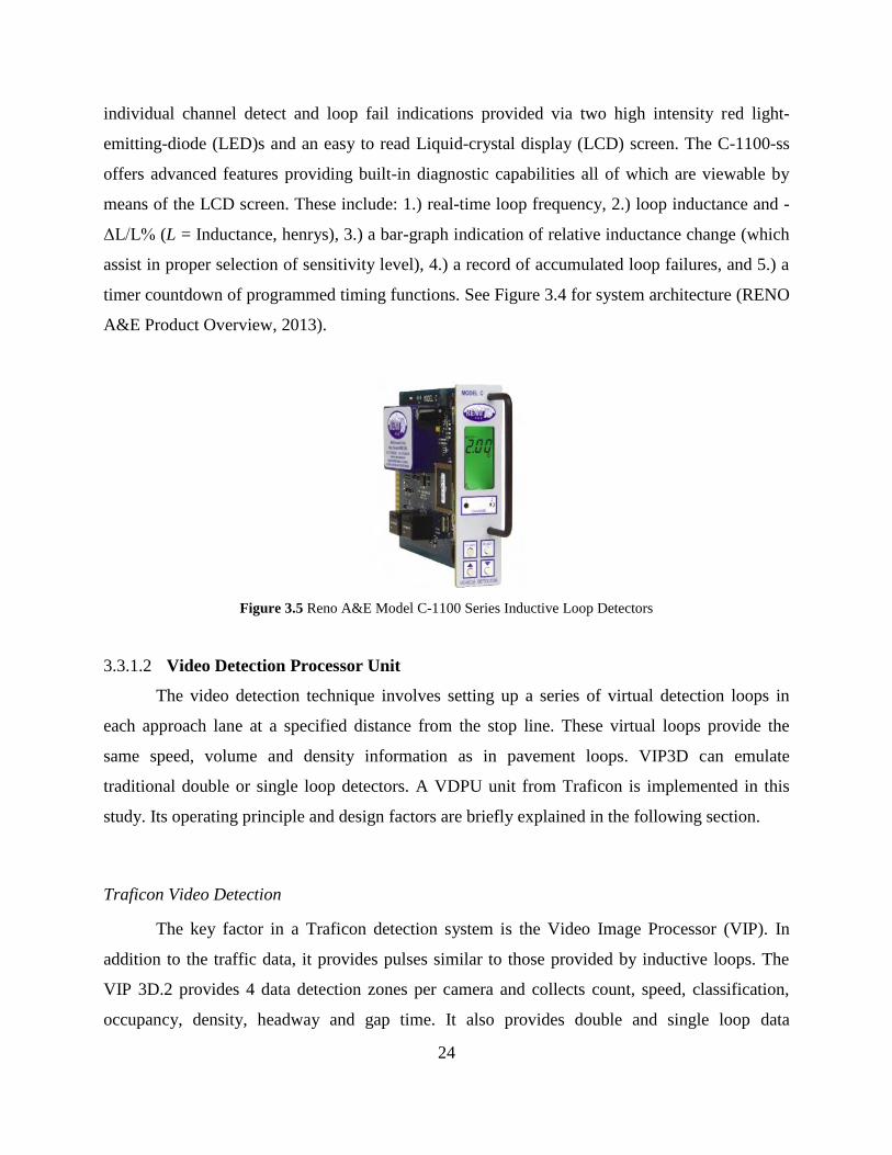
24

individual channel detect and loop fail indications provided via two high intensity red light-

emitting-diode (LED)s and an easy to read Liquid-crystal display (LCD) screen. The C-1100-ss

offers advanced features providing built-in diagnostic capabilities all of which are viewable by

means of the LCD screen. These include: 1.) real-time loop frequency, 2.) loop inductance and -

ΔL/L% (L = Inductance, henrys), 3.) a bar-graph indication of relative inductance change (which

assist in proper selection of sensitivity level), 4.) a record of accumulated loop failures, and 5.) a

timer countdown of programmed timing functions. See Figure 3.4 for system architecture (RENO

A&E Product Overview, 2013).

Figure 3.5 Reno A&E Model C-1100 Series Inductive Loop Detectors

Video Detection Processor Unit 3.3.1.2

The video detection technique involves setting up a series of virtual detection loops in

each approach lane at a specified distance from the stop line. These virtual loops provide the

same speed, volume and density information as in pavement loops. VIP3D can emulate

traditional double or single loop detectors. A VDPU unit from Traficon is implemented in this

study. Its operating principle and design factors are briefly explained in the following section.

Traficon Video Detection

The key factor in a Traficon detection system is the Video Image Processor (VIP). In

addition to the traffic data, it provides pulses similar to those provided by inductive loops. The

VIP 3D.2 provides 4 data detection zones per camera and collects count, speed, classification,

occupancy, density, headway and gap time. It also provides double and single loop data

25

simulation. Queue length measurements and directional counts on the intersection can also be

conducted (Traficon Product Overview, 2013). The system architecture for VDPUs is very

similar to the system architecture for ILDs shown in Figure 3.4. The architecture differs from the

ILD one only in the use of cameras in place of loop coils as shown in Figure 3.7.

Cabinet VIP 3D2 unit

Figure 3.6 Traficon VIP3D.2 sensor

26

Figure 3.7 VDPU System Architecture

Magnetometer 3.3.1.3

Magnetometers operate by detecting changes in the Earth’s magnetic field caused by the

metal objects traveling over them. Sensys magnetometer pucks are battery operated units placed

in the roadway which communicate via radio with receivers that communicate that data to

controllers for processing. Sensys pucks are discussed in greater detail under reidentification in

Section 3.3.2.3.

3.3.2 Vehicle Re-identification Technologies

A wide range of vehicle re-identification technologies are now in use. In this study, six

different vehicle re-identification technologies are used, which can be classified into three

categories: automated license plate recognition, Bluetooth / WiFi MAC address matching and

magnetic signature matching. Their operating principles and design factors are discussed in the

following sections.

27

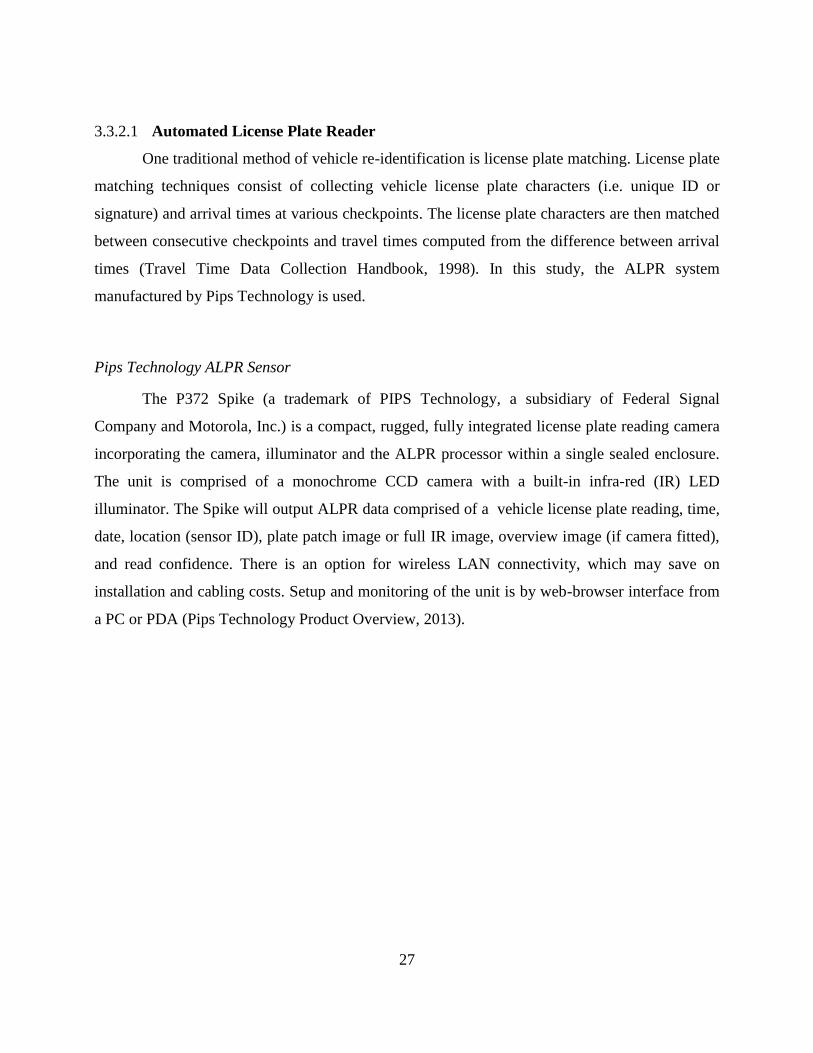
Automated License Plate Reader 3.3.2.1

One traditional method of vehicle re-identification is license plate matching. License plate

matching techniques consist of collecting vehicle license plate characters (i.e. unique ID or

signature) and arrival times at various checkpoints. The license plate characters are then matched

between consecutive checkpoints and travel times computed from the difference between arrival

times (Travel Time Data Collection Handbook, 1998). In this study, the ALPR system

manufactured by Pips Technology is used.

Pips Technology ALPR Sensor

The P372 Spike (a trademark of PIPS Technology, a subsidiary of Federal Signal

Company and Motorola, Inc.) is a compact, rugged, fully integrated license plate reading camera

incorporating the camera, illuminator and the ALPR processor within a single sealed enclosure.

The unit is comprised of a monochrome CCD camera with a built-in infra-red (IR) LED

illuminator. The Spike will output ALPR data comprised of a vehicle license plate reading, time,

date, location (sensor ID), plate patch image or full IR image, overview image (if camera fitted),

and read confidence. There is an option for wireless LAN connectivity, which may save on

installation and cabling costs. Setup and monitoring of the unit is by web-browser interface from

a PC or PDA (Pips Technology Product Overview, 2013).

28

Figure 3.8 Pips P327 Spike ALPR sensor

MAC Address Matching Technology 3.3.2.2

Bluetooth-based travel time measurement is one of the emerging methods of vehicle re-

identification. This method involves identifying and matching the unique Media Access Control

or Media Access Control (MAC) address of Bluetooth-enabled devices carried by motorists as

they pass a detector location. As with ALPRs, the difference in time between the two

observations yields the travel time. This approach relies on having a device with an active

Bluetooth or Wi-Fi adapter in the sensor’s detection range. In this Bluetooth technology from two

different manufacturers are evaluated.

BlueTOAD Bluetooth Sensors

BlueTOAD (a trademark of TrafficCast) is a Bluetooth MAC address detection system

developed by TrafficCast International (TCI). The BlueTOAD device consists of the MAC

address reader, a power source, and a communication source. The BlueTOAD devices are

capable of Ethernet or cellular communication. The options for power are hard wire or solar

29

power. The BlueTOAD cellular solar power option requires a service provider in order to

communicate with the TCI servers. The Ethernet option allows for a direct connection to a hard

wired network. The hard wire option can be connected to any power source capable of supporting

110V of AC power (TrafficCast Product Overview, 2013). The BlueTOAD cellular Solar Power

50W is used in this research, shown in Figure 3.9.

The device reads the MAC address broadcast from any active Bluetooth device and sends

the time of the read and MAC information to the TrafficCast central processing server to

calculate travel times. TrafficCast then filters the data to remove outliers and provides the

information to clients via a web interface. The TrafficCast secure cyber-center processes the data

collected by BlueTOAD devices. Data can be viewed in real-time or analyzed historically

through a BlueTOAD web interface, which provides travel times, road speeds, and MAC address

detection counts.

30

Figure 3.9 BlueTOAD sensor design and components

BlipTrack Bluetooth Sensors

BlipTrack (a trademark of Blip Systems) is a Bluetooth sensor developed by Blip

Systems. The BlipTrack Traffic sensor has 3 Bluetooth antennae including 2 directional antennae

31

and 1 omnidirectional. The size of the detection zone varies from 70-200m on either side of the

sensor along the road. When using 3 Bluetooth radios, BlipTrack has a 3 times greater chance of

detecting a Bluetooth device and also covers an area more than 3 times as large as a single radio

solution. BlipTrack also has built-in 3G and LAN connectivity for easy upload and a GPS sensor

for auto positioning. The BlipTrack Bluetooth Traffic sensor uses 220V power with a battery

backup (Blip Systems A/S Product Overview, 2013). The sensor configuration and components

are shown in Figure 3.10.

BlipTrack works by detecting Bluetooth devices in proximity to a BlipTrack Access

Point. The sensors relay each detection event to a central server using their 3G connection. Each

detection event is comprised of the MAC address of the detected device and the detection

timestamp. Blip Systems then filters the data to remove outliers and provides the information to

clients via a web interface. BlipTrack has a graphical interface with Google Maps integration,

widgets and a wide range of real-time and historical analytical tools, which provides travel times,

road speeds, and MAC address detection counts.

Figure 3.10 BlipTrack sensor design and components

32

The new model of BlipTrack sensor incorporates a WiFi processor into the design. In this design

an external WiFi unit can be connected to the Bluetooth unit. The joint WiFi/Bluetooth unit has

the capability of detecting the MAC addresses transmitted by both WiFi and Bluetooth-enabled

devices (Blip Systems A/S Product Overview, 2013). The architecture of BlipTrack solution is

shown in Figure 3.12.

Figure 3.11 BlipTrack WiFi sensor design and components

WiFi

Bluetooth

33

Figure 3.12 Architecture of BlipTrack solution

Magnetic Signature Matching 3.3.2.3

This method relies on matching vehicle signatures from wireless sensors. The sensors

provide a noisy magnetic signature of a vehicle and the precise time when it crosses the sensors.

A match (re-identification) of signatures at two locations gives the corresponding travel time of

the vehicle.

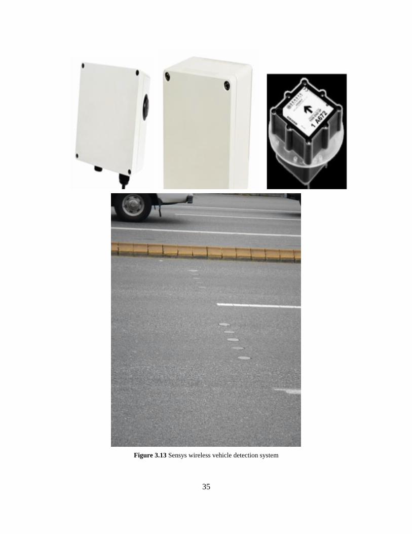
Sensys Wireless Vehicle Detection System

The Sensys (a trademark of Sensys Networks, Inc.) wireless vehicle detection system uses

pavement-mounted magnetic sensors to detect the presence and movement of vehicles. The

34

magneto-resistive sensors are wireless, transmitting their detection data in real-time via low-

power radio technology to a nearby Sensys access point that then relays the data to one or more

local or remote traffic management controllers and systems.

The Sensys VSN240-F is an in-pavement wireless vehicle sensor designed for permanent

deployment in all traffic conditions from freeways to intersections to parking lots to gates. The

VSN240-F detects vehicular traffic and reports it back to an AP240 access point. Each sensor

node contains a 3 axis magnetometer, microprocessor, memory, low power radio and batteries

within a watertight case. After a vehicle passes over the sensor array, each sensor transmits its

unique magnetic signature information to a wireless access point located within 150 feet of the

array. If the sensor array is located outside this range, a battery operated repeater can retransmit

the information up to 1,000 feet away. The access point collects the data from each sensor or

repeater and retransmits the information to a data archiving server. Once the information is

collected by the data archive server, it is used by the re-identification engine for travel time

analysis. A Sensys access point (AP240-EC) is an intelligent device operating under the Linux

operating system that maintains two-way wireless links to an installation’s sensors and repeaters,

establishes overall time synchronization, transmits configuration commands and message

acknowledgements, and receives and processes data from the sensors. The Sensys access point

then uses either wired or wireless network connections (or both) to relay the sensor detection data

to a roadside traffic controller or remote server, traffic management system, or other vehicle

detection application. A Sensys repeater (RP240-B) extends the range and coverage of an

installation’s access point. The three devices may be seen Figure 3.13 (Sensys Networks Product

Overview, 2013). Architecture of Sensys magnetometers are presented in Appendix I.

35

Figure 3.13 Sensys wireless vehicle detection system

36

3.3.3 3rd Party Inrix Data

Inrix aggregates traffic-related information from millions of GPS-enabled vehicles and

mobile devices, traditional road sensors and hundreds of other sources. The result is a real-time,

historical and predictive traffic services on freeways, highways, and secondary roadways,

including arterials and side streets (Inrix, 2013). For this research historical Inrix data was

acquired through the WSDOT contract with Inrix.

38

Chapter 4 Evaluation Frame Work

Considering the extensive sensing capabilities installed along SR 522 and I-90,

performing a systematic comparison of the available technologies is a matter of selecting the

appropriate metrics, pulling the data from the various sources and then performing an error

analysis. In this study, a framework has been designed and implemented to evaluate the accuracy

and reliability of the various technologies.

4.1 Error and Reliability Matrix

In order to evaluate the accuracy and reliability of travel time estimates obtained by

various ATIS technologies, three types of analysis are conducted.

First, the distributions of the travel time data and sample rates relative to the ground truth

and other ATIS technologies are compared.

Second, a number of accuracy measures are used to provide a numerical evaluation of the

error associated with each of the technologies for travel time estimation.

In order to use a consistent data format, the comparisons are made based on 5 minutes

aggregated travel time and capture rates. The two datasets that were not available on a five

minute basis were BlueTOAD capture rates and Inrix capture rates. BlueTOAD capture rates

were available at 15 minute intervals and divided by 3 to match up to the other systems as closely

as possible. The Inrix data does not include a capture rate. In this study the ALPR data are used

as the ground truth the accuracy analysis and baseline for vehicle sampling counts.

4.1.1 Data Distribution

Distributions of the data around the ground truth are compared using time plots. This

enables readers to get an overview of the distributions of the data relative to the ground truth.

39

4.1.2 Travel Time Accuracy and Error

A number of accuracy metrics are used to represent the error. In these metrics, error is the

difference between the observations and the ground truth travel time. These accuracy measures

are:

1. Mean Absolute Deviation (MAD) (also known as the mean absolute error) – the average

of errors.

∑| |

(4.1)

The number of observations

The corresponding ground truth travel time, i

The ATIS estimated travel time

2. Mean Percent Error (MPE) – the average percentage difference between the estimate and

ground truth.

∑

( )

(4.2)

3. Mean Absolute Percent Error (MAPE) – the average absolute percentage difference

between the estimate and ground truth.

∑

| |

(4.3)

4. Root Mean Squared Error (RMSE) – the square root of the average of the squared errors.

40

√

∑( )

(4.4)

There are reasons to use each error measurement methodology. The MAD is a good

indication of how much error should be expected from an average reading, but does not indicate

whether the results are consistently high or low. The MPE will indicate if there is systematic bias

to the error, i.e. if readings are consistently high or low, but will allow positive and negative

errors to cancel each other out. The MAPE is a combination of MAD and MPE, indicating

average magnitude of error. The RMSE gives a good indication of whether there are many small

errors or a few larger errors.

A good approach to judging sensor accuracy is to look at the MAD to judge the expected

magnitude of error. Then examine the MPE to determine whether there are systematic biases to

the data. Note that for travel time it is reasonable to expect errors to be skewed toward longer

travel times in most cases, since travel time underestimation is bounded on the lower end by zero.

This is particularly true for SR 522 where individual segment free flow travel times are on the

order of a minute and the whole corridor can be traversed in five minutes. The MAPE is useful to

find the relative magnitude of the error. Finally, the RMSE is useful in determining whether a

few large errors or many smaller errors are occurring. Between the four measures of error, a user

can determine the magnitude of error, its biases, the relative impact of that error and the

magnitude of the typical error.

4.1.3 Data Analysis Resolutions

Since the reporting intervals of the data available vary among different technologies,

analyses are conducted for three different levels of resolutions. The three levels of resolution

considered for evaluation are: hourly, daily, and monthly basis. It is important to consider the

various temporal resolutions of data analysis while evaluating the various sensors. When looking

at weekly data, the consistency of the travel times across multiple days provides a good measure

of the highs and lows that should be expected for travel times between the two intersections.

Monthly data can be used to analyze whether the travel times between the two intersections are

41

consistent and cyclical. By analyzing monthly data, it is also possible to indicate some days that

recorded significantly longer travel times than others. This may be indicative of incidents

blocking traffic. Further examinations would need to be undertaken to establish causal factors.

4.2 Data Availability

Data collection on SR 522 started on December 2012 and continued until June 2013.

Table 4.1 and Table 4.2 display the time intervals when data were collected for both westbound

and eastbound respectively. As can be seen, ALPR and Sensys data were only available on

westbound, hence this direction will be used as the basis of travel time accuracy analysis. The

gaps shown on the tables represent time periods that a technology was not either installed or was

not working.

In the time span between April 5th


2013 all systems collected data

side-by-side. The most data overlap between various systems occurred during this time period

which provided a sufficiently large dataset for analysis. Therefore, this time period allows

comparing the accuracy of data collected by all different systems in terms of travel time and

capture rate (with the partial exception of BlueTOAD data which only reports match rates at 15

minute intervals). The 5 minute aggregated travel time and sample counts were used as the basis

of analysis. Due to the difference of traffic pattern on weekends and working days, this study

uses traffic data collected on weekdays for conducting error analyses.

Due to the differences between sensor availability and type of data collected by these

sensors, the type of analyses conducted for eastbound and westbound varies. Sensor availability

and types of data analysis for westbound and eastbound on SR 522 are summarized in Table 4.1

and Table 4.2, respectively. ALPR data are used as ground truth both for travel time analysis and

sample count comparison. Inrix data does not include sample counts, so that system is excluded

from sample count analysis.

When it comes to eastbound SR 522, there is no ALPR data that lines up with the other

systems in the eastbound direction. This prevents an analysis based on using the ALPR system

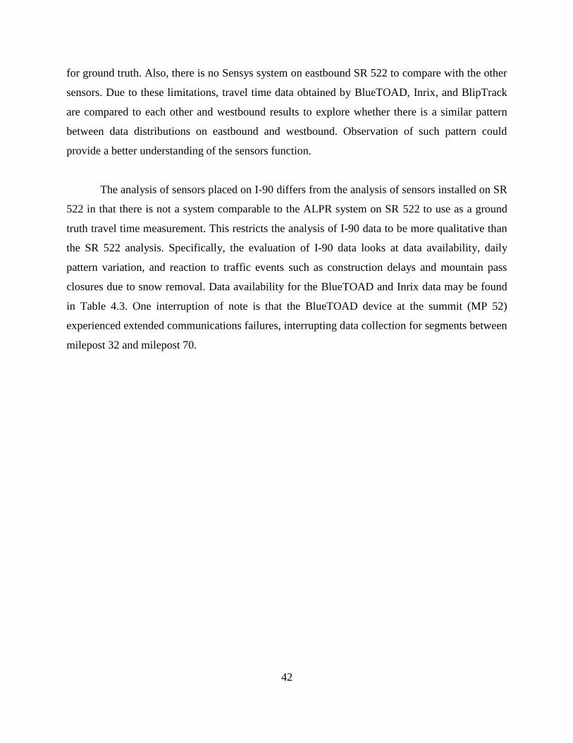
42

for ground truth. Also, there is no Sensys system on eastbound SR 522 to compare with the other

sensors. Due to these limitations, travel time data obtained by BlueTOAD, Inrix, and BlipTrack

are compared to each other and westbound results to explore whether there is a similar pattern

between data distributions on eastbound and westbound. Observation of such pattern could

provide a better understanding of the sensors function.

The analysis of sensors placed on I-90 differs from the analysis of sensors installed on SR

522 in that there is not a system comparable to the ALPR system on SR 522 to use as a ground

truth travel time measurement. This restricts the analysis of I-90 data to be more qualitative than

the SR 522 analysis. Specifically, the evaluation of I-90 data looks at data availability, daily

pattern variation, and reaction to traffic events such as construction delays and mountain pass

closures due to snow removal. Data availability for the BlueTOAD and Inrix data may be found

in Table 4.3. One interruption of note is that the BlueTOAD device at the summit (MP 52)

experienced extended communications failures, interrupting data collection for segments between

milepost 32 and milepost 70.

43

Table 4.1 Data Availability on SR-522 Westbound

44

Table 4.2 Data Availability on SR-522 Eastbound

45

Table 4.3 Data availability by month and system for I-90

46

4.2.1 Types of Data

Due to the differences between sensor availability and type of data collected by these

sensors, the type of analysis conducted for eastbound and westbound varies. Sensor availability

and types of data analysis for eastbound and westbound on SR 522 are summarized in Table 4.4.

ALPR data are used as ground truth both for travel time analysis and sample count comparison.

Table 4.4 Data availability and type of analysis on westbound and eastbound SR 522

Data available on I-90 is shown in Table 4.5. Due to the lack of ground truth data on this corridor

travel time analyses are restricted to qualitative rather than quantitative analysis.

47

Table 4.5 Data availability and type of analysis on westbound and eastbound I-90

4.3 Data analysis and discussions for SR 522

Evaluations of various technologies are conducted in terms of sample count and accuracy of

travel time estimation. The following sections present the results of data analysis based on visual

and numerical methods.

4.3.1 Sample Count

Sample counts and the corresponding penetration rate are two important factors for evaluating

various travel time technologies. These represent the proportion of the actual traffic flow being

captured by the sensors. The results of the sample count analysis for westbound and eastbound

are presented in the following sections.

Westbound sample count 4.3.1.1

The results of sample count on westbound for the period between April 5th

, 2013 through June

8th

, 2013 are summarized in Table 4.6. As stated in section 4.1, the ALPR sample counts are used

as the baseline. In this context, penetration rates are computed by dividing sample counts of

various systems by the corresponding ALPR value.

(4.5)

48

According to Table 4.6, on average, the penetration rate of Sensys is identical ( 103%) to the

sample captured by ALPR. This is followed by Blip-Combined with more than 28% of the ALPR

captures, Blip-WiFi with 17% and Blip-BT with 12% of ALPR capture rates. This also indicates

that by combining Bluetooth and WiFi technologies, it is possible to capture twice as many

samples compared to the use of a single technology. The BlueTOAD capture rate is 6%.

Figure 4.1 shows the average penetration rate over the analysis period (April 5th

, 2013 through

June 8th

, 2013) for various sensors on the westbound links. In order to give an overview of the

sample counts variations over the weekdays, Figure 4.2, Figure 4.3, and Figure 4.4 display the

capture rates of the various systems on SR 522 westbound links for a one week period May 1st,

2013 through May 8th

, 2013. Comparing the penetration rates of the various sensors on the three

links shows that despite the differences in traffic flow on the various links, the ratios are similar

which indicates the reliability of the sensor detection results.

Although Blip-BT, Blip-WiFi and Blip-Combined, and BlueTOAD have a significantly lower

penetration rates compared to ALPR and Sensys, they still demonstrate responsiveness to the

variations in traffic volumes during the day. BlueTOAD data in Figure 4.2, Figure 4.3, and

Figure 4.4 is blockier in profile due to being aggregated in 15-minute intervals instead of the 5-

minute interval used by other sensor systems. In order to represent the BlueTOAD data on the

same scales as the other systems, the BlueTOAD capture data was divided by 3, which may cause

its capture rate to be underrepresented in low volume conditions due to rounding.

49

Table 4.6 Sample counts on westbound SR 522 during April 5th


2013

Note: ALPR capture rate is defined as 100% with all other sensors judged relative to ALPR

50

Figure 4.1 Capture rate comparison on westbound SR 522 between April 5th, 2013 through June 8th 2013

51

Figure 4.2 Comparing capture rate of different systems from 83rd Pl. NE to 68th Ave. NE (WB) for May 1st, 2013 through May 8

th, 2013

Figure 4.2 shows the overlaid profiles of capture rate for various sensors on 83rd

Pl. NE to 68th

Ave. NE (WB) for May 1st, 2013 through May 8

th, 2013. It clearly shows that Sensys and ALPR have higher capture rates,

followed by Blip-Combined, Blip-WiFi and Blip-BT, and BlueTOAD. Figure 4.2 shows that regardless of the variations in capture rates for different systems; all of the systems were capable of registering the flow variation

for peak and off-peak over the course of weekdays and weekends.

52

Figure 4.3 Comparing capture rate of different systems from 68th Ave. NE to SR 104 (WB) for May 1st, 2013 through May 8th, 2013

Figure 4.3 shows the overlaid profiles of capture rate for various sensors on 68th Ave. NE to SR 104 (WB) for May 1st, 2013 through May 8

th, 2013. It clearly shows that Sensys and ALPR have the higher capture rate which

followed by Blip-Combined, Blip-WiFi and Blip-BT, andBlueTOAD. Figure 4.3 shows that all of the systems were capable of registering the flow variation for peak and off-peak over the course of weekdays and weekends.

53

Figure 4.4 Comparing capture rate of different systems from SR 104 to NE 153rd St. (WB) for May 1st, 2013 through May 8th, 2013

Figure 4.4 shows the overlaid profiles of capture rate for various sensors from SR 104 to NE 153rd

St. (WB) for May 1st, 2013 through May 8

th, 2013. It clearly shows that Sensys and ALPR have the higher capture rate which

followed by Blip-Combined, Blip-WiFi and Blip-BT, and BlueTOAD. Figure 4.4 shows that all of the systems were capable of registering the flow variation for peak and off-peak over the course of weekdays and weekends.

54

When examining the various technologies, it is important to understand how well each

technology performs in relative and absolute terms. While the ALPR system was chosen as a

ground truth reference for travel time, the ALPR system was not designed as a volume

measurement system. In the following figures volumes from each system that provides a volume

measurement and the match rates for each system are shown. For comparison purposes, the

advance loop detectors are shown as well as the Traficon system volumes at the 83rd

Pl. NE and

68th

Ave. NE intersections.

The placement of each system will have some implications to be taken into account when

examining this data. Specifically, the advance loop detectors are upstream of the signal on the

through movement lanes, while the ALPR, Sensys and Traficon systems are placed on the

downstream side of the intersection. Traficon and Sensys counts generally agree, though they are

not identical and Sensys does report marginally lower volumes.

The ALPR volumes follow the trends seen in the other three volume data sets, but are

generally the lowest reported volumes. This is unsurprising since the ALPR system was not

designed for volume data collection. A number of factors such as vehicle height, spacing, and

license plate cleanliness can affect the ALPR’s ability to read a license plate. Loop detectors,

magnetometers and VIP units are not trying to read a small target, like a license plate, and have

generally more robust detection.

The placement of the advance loop detectors is likely to affect volume counts. The

placement of the loop detectors means that only entering through vehicles are counted, left and

right turning vehicles from the cross street are not counted. Additionally, the advance loop

detectors may be subject to queuing and intersection signal timing impacts. With all of these

factors it is unsurprising that the advance detectors consistently report the second lowest

volumes.

55

Figure 4.5 Westbound Volume and Capture Rates for Wednesday May 1, 2013 from 83rd Place NE to 68th Avenue NE

In Figure 4.5 the number of matches reported by each system are represented by solid lines. Dotted lines are used to represent the volumes reported at the upstream intersection and dashed lines are used to represent the

volume at the downstream intersection. Sensys volumes and match rates are shown in green. ALPR volumes and match rates are shown in dark gray. The BlueTOAD match rate is shown in dark blue. The Blip Bluetooth,

WiFi and Combined match rates are shown in purple, light blue and orange, respectively. The 83rd Place NE intersection includes Traficon and advance loop detectors upstream of the intersection included here for volume

counts, shown by red and magenta dotted lines, respectively. The 68th Avenue NE intersection also includes Traficon and advance loop detectors on the upstream side of the intersection included here for volume counts,

shown by red and magenta dashed lines, respectively. Readers should note that the Sensys and ALPR systems report significantly higher match rates than the other systems. Also of interest is that the two Bluetooth systems

perform comparably with regards to match rates. The additional matches reported by Blip-Combined are largely a result of the added WiFi sensors.

56

Figure 4.6 Westbound Volume and Capture Rates for Wednesday May 1, 2013 From 68th Avenue to SR-104 Junction


volume at the downstream intersection. Sensys volumes and match rate are shown in green. ALPR volumes and match rate are shown in dark gray. The BlueTOAD match rate is shown in dark blue. The Blip Bluetooth, WiFi

and Combined match rates are shown in purple, light blue and orange, respectively. The 68th Avenue NE intersection includes Traficon and advance loop detectors upstream of the intersection included here for volume

counts, shown in by red and magenta dashed lines, respectively. Readers should note that the Sensys and ALPR systems report significantly higher match rates than the other systems. The ALPR system appears to be more

effective during the morning peak. Also of interest is that the two Bluetooth systems perform comparably with regards to match rates. The additional matches reported by Blip-Combined are a result of the added WiFi sensors.

The WiFi sensors also appear to have stronger morning and evening peaks than Bluetooth.

57

Figure 4.7 Westbound Volume and Capture Rates for Wednesday May 1, 2013 From SR-104 Junction to NE 153rd Street


volume at the downstream intersection.Readers should note that the Sensys and ALPR systems report significantly higher match rates than the other systems. Also of interest is that the two Bluetooth systems perform

comparably with regards to match rates. The additional matches reported by Blip-Combined are a result of the added WiFi sensors. The WiFi sensors also appear to have stronger morning and evening peaks than Bluetooth.

58

Eastbound Sample Count 4.3.1.2

The sample count results for eastbound for the period of April 5th


,

2013 are summarized in Table 4.7. One notable point is that similar to the westbound sample

counts, the Blip-Combined capture rate is about two times higher than the capture rates of the

Blip-BT and Blip-WiFi. There are more Blip-WiFi matches than Blip-BT matches. Results show

that overall there are 20% more devices seen by the WiFi sensor than Bluetooth. The WiFi

devices detected are primarily iPhones, Android and Windows Phone 8 devices. These devices

are not detected by the Bluetooth sensor, due to specific implementation of the Bluetooth

software in these phones. So the WiFi detections could well complement the Bluetooth data.

Table 4.7 Sample counts on eastbound SR 522 over period of April 5th


, 2013

Figure 4.8, Figure 4.9, and Figure 4.10 display the capture rate of various systems on SR 522

eastbound links for the period of one week (May 1st, 2013 through May 8

th, 2013). As seen for

westbound, even though Blip-BT, Blip-WiFi and Blip-Combined have significantly lower

capture rates but they are capable of representing the variations of traffic flow during the day.

This could be seen by peaks during morning and afternoon on weekdays and likewise peaks on

around noon on the weekends. However, due to lack of ground truth for this direction it is not

possible to verify the travel time results.

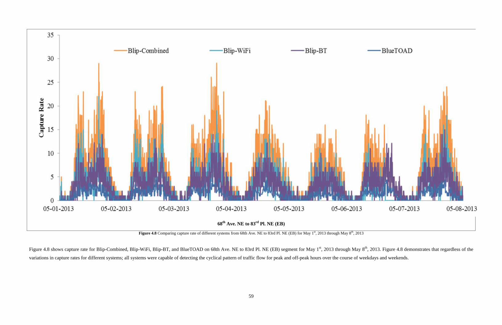
59

68th

Ave. NE to 83rd

Pl. NE (EB)

Figure 4.8 Comparing capture rate of different systems from 68th Ave. NE to 83rd Pl. NE (EB) for May 1st, 2013 through May 8

th, 2013

Figure 4.8 shows capture rate for Blip-Combined, Blip-WiFi, Blip-BT, and BlueTOAD on 68th Ave. NE to 83rd Pl. NE (EB) segment for May 1st, 2013 through May 8

th, 2013. Figure 4.8 demonstrates that regardless of the

variations in capture rates for different systems; all systems were capable of detecting the cyclical pattern of traffic flow for peak and off-peak hours over the course of weekdays and weekends.

60

SR 104 to 68th

Ave. NE (EB)

Figure 4.9 Comparing capture rate of different systems from SR 104 to 68th Ave. NE (EB) for May 1st, 2013 through May 8

th, 2013

Figure 4.9 shows capture rate for Blip-Combined, Blip-WiFi, Blip-BT, and BlueTOAD on SR 104 to 68th

Ave. NE (EB) segment for May 1st, 2013 through May 8

th, 2013. Figure 4.9 shows that regardless of the variations in

capture rates for different systems; all systems were capable of detecting the cyclical pattern of traffic flow for peak and off-peak hours over the course of weekdays and weekends.

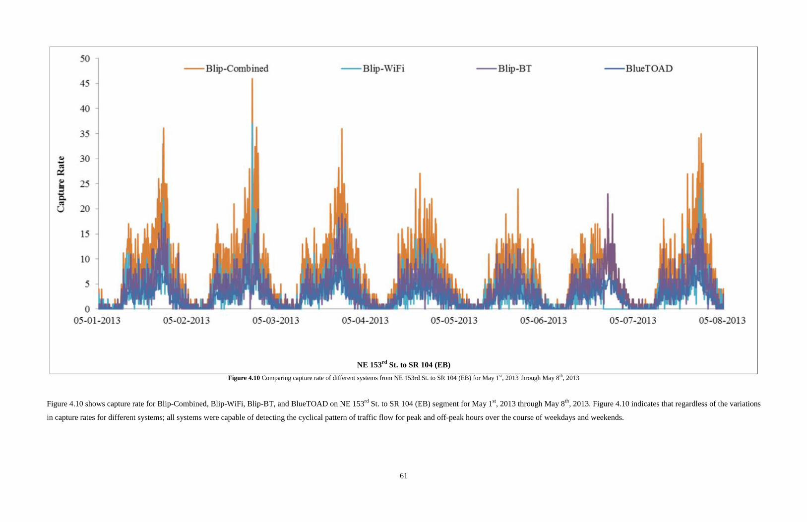
61

NE 153rd

St. to SR 104 (EB)

Figure 4.10 Comparing capture rate of different systems from NE 153rd St. to SR 104 (EB) for May 1st, 2013 through May 8

th, 2013

Figure 4.10 shows capture rate for Blip-Combined, Blip-WiFi, Blip-BT, and BlueTOAD on NE 153rd

St. to SR 104 (EB) segment for May 1st, 2013 through May 8

th, 2013. Figure 4.10 indicates that regardless of the variations

in capture rates for different systems; all systems were capable of detecting the cyclical pattern of traffic flow for peak and off-peak hours over the course of weekdays and weekends.

62

4.4 Travel Time

The accuracy and reliability of the travel time estimations are critical parameters for

evaluating various sensor technologies. Due to the difference in data availability for westbound

and eastbound directions, the results of the travel time analyses are presented separately by

direction. On westbound, in order to provide a better foundation for comparing accuracy of

different systems, analyses are conducted for different time resolutions. The accuracy analysis

looks at the overall accuracy for April 5th


, 2013, and also on a 24 hour

daily resolution for all Wednesdays in this period (refer to Figure 4.14, Figure 4.15, and Figure

4.16). However, on eastbound due to the lack of ALPR data to act as ground truth data during the

analysis period, analysis of the eastbound data is limited to descriptive statistics.

4.4.1 Westbound Travel Time

Travel time plots for the three segments on SR 522 westbound are shown in Figure 4.11,

Figure 4.12, and Figure 4.13 for the analysis period of May 1st, 2013 through May 8

th, 2013. The

consistency of the travel times across the week provides a good measure of the highs and lows

that should be expected for travel times on the three segments. The weekly data demonstrates that

the travel times on all three corridors are consistent and cyclical. May 6th

is a Saturday and May

7th

is a Sunday. Saturday and Sunday have reduced peaks centered at midday. The regular

workdays have earlier and longer peaks that have a minor peak in the morning and a major one in

the evening for the 83rd

Pl. NE to 68th

Ave. NE segment and narrow major peaks in morning and

wider evening peaks for the other two segments. These results are in accordance with

expectations based on local traffic and commuter patterns.

63

83rd

Pl. NE to 68th

Ave. NE (WB)

Figure 4.11 Travel time plot for 83rd

Pl. NE to 68th

Ave. NE (WB) for May 1st, 2013 through May 8

th, 2013

Figure 4.11 shows the overlaid travel times for all the sensors from 83rd

Pl. NE to 68th

Ave. NE (WB) over the course of a week from May 1st, 2013 through May 8

th, 2013. It is clear that all the sensors are capable of

responding to the cyclical pattern of travel time over weekdays and weekends and also for the morning and afternoon peaks. Over the peak and off-peak hours all sensors follow the ALPR pattern and thus have a strong

overlap with the ground truth. However, Inrix data tend to significantly underestimate the travel time. A number of gaps or low travel times were reported for all methods (except Inrix) over the mid night hours.

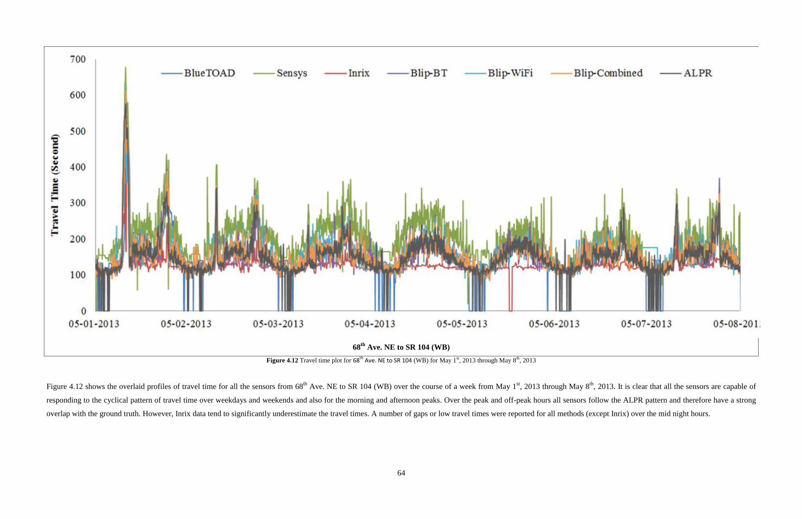
64

68th

Ave. NE to SR 104 (WB)

Figure 4.12 Travel time plot for 68th

Ave. NE to SR 104 (WB) for May 1st, 2013 through May 8

th, 2013

Figure 4.12 shows the overlaid profiles of travel time for all the sensors from 68th

Ave. NE to SR 104 (WB) over the course of a week from May 1st, 2013 through May 8


responding to the cyclical pattern of travel time over weekdays and weekends and also for the morning and afternoon peaks. Over the peak and off-peak hours all sensors follow the ALPR pattern and therefore have a strong

overlap with the ground truth. However, Inrix data tend to significantly underestimate the travel times. A number of gaps or low travel times were reported for all methods (except Inrix) over the mid night hours.

65

SR 104 to NE 153rd

St. (WB)

Figure 4.13 Travel time plot from SR 104 to NE 153rd St. (WB) for May 1st, 2013 through May 8th, 2013

Figure 4.13 shows the overlaid profiles of travel time for all the sensors from SR 104 to NE 153rd

St. (WB) over the course of a week from May 1st, 2013 through May 8


responding to the cyclical pattern of travel time over weekdays and weekend and also for the morning and afternoon peaks. Over the peak and off-peak hours all sensors follow the ALPR pattern and have a strong overlap with

the ground truth. However, Inrix data tend to significantly overestimate the travel time during off-peak intervals. A number of gaps or low travel times have also been reported for all methods (except Inrix) over the mid night

hours.

66

Travel Time Accuracy Analysis for Westbound 4.4.1.1

In order to provide a daily overview of the accuracy of the travel time estimated by

various technologies, the MAPE for all westbound segments are calculated for Wednesdays over

the of two month period from April 5, 2013 to June 8, 2013. The results of the MAPE analysis

are shown in Figure 4.14, Figure 4.15, and Figure 4.16. The patterns observed for the three

segments are different; however, it can be seen that, in general, during the peak hours estimations

tend to be more biased and the percentage of errors increase. For all three segments, during the

peak hours Inrix tends to be more biased and less accurate than the Sensys and Blip-BT, Blip-

WiFi and Blip-Combined. For the SR 104 to NE 153rd

St. segment BlueTOAD also shows

significant bias for the morning peak. BlueTOAD also show significant bias in the overnight

hours for the 83rd

Pl. NE to 68th

Ave. NE segment.

67

Figure 4.14 The MAPE variation for 83rd Pl. NE to 68th Ave. NE (WB) over 24 hours on Wednesdays over the period of April 5th


, 2013

Figure 4.14 presents the variation of MAPE over 24 hours for Wednesdays over the period of April 5th


, 2013 at for 83rd Pl. NE to 68th Ave. NE (WB). It is clear that the accuracy of the various systems’

estimated travel times varies between peak and off-peak hours. This is especially true of the morning peak from 8am to 9am. As shown, BlueTOAD has a lower MAPE over the course of the day followed by Blip-Combined,

Blip-BT, Blip-WiFi, Sensys and Inrix. Compared to other systems, Inrix has significantly lower accuracy during the day and BlueTOAD shows significantly lower accuracy during the night.

68

Figure 4.15 The MAPE variation from68th Ave. NE to SR 104 (WB) over 24 hours on Wednesdays over the period of April 5th


, 2013



, 2013 at 68th

Ave. NE to SR 104 (WB). The accuracy of the estimated travel times varies over the

day, though not as significantly as on the 83rd

Pl. NE to 68th

Ave. NE segment. As shown Blip-BT, Blip-WiFi, and Blip-Combined estimate travel time with approximately 15% error over the course of the day. Although,

accuracy of travel time estimated by BlueTOAD fluctuates between peak and off-peak hours, in off-peaks it can estimate travel time with less than 15% error which rises to 70% error during peak. In this segment, Sensys

performance on this segment is acceptable overnight, with an error spike in the peak hour and just over the acceptable error threshold over the day. For this segment, Inrix has a modest accuracy, generally competitive with the

other systems.

69

Figure 4.16 The MAPE variation from SR 104 to NE 153rd St. (WB) over 24 hours on Wednesdays over the period of April 5

th, 2013 through June 8

th, 2013



, 2013 from SR 104 to NE 153rd St. (WB). It is clear that the accuracy of the estimated travel time

by various systems varies between peak and off-peak hours. As shown Sensys and BlueTOAD have lower accuracy during the morning peak followed by Blip-Combined and Blip-BT with Blip-WiFi being the most accurate.

During the morning peak there is a significant rise in the BlueTOAD and Sensys error rates which leveled out for the rest of the day. Inrix data for this segment was subject to significant error.

70

In order to further explore this pattern, data collected between 9am-10am (off-peak) on

Wednesdays during two months (April 5th


, 2013) are analyzed. Table 4.8

presents descriptive statistics of the collected data. As seen in Table 4.8, the average ALPR travel

time is closely estimated by all sensors. Table 4.8 presents the travel time samples recorded by

each system grouped by segment as well as the sample penetration rate compared to the ALPR

system. The travel time standard deviation in seconds, minimum travel time, 1st quartile, median,

mean, 3rd

quartile and maximum are also presented.

To evaluate the accuracy of the sensors on an hourly basis, the MAPE for each sensor on

each segment of the corridor is calculated for 9am-10am (off-peak) on Wednesdays during two

months (April 5th


, 2013), as seen in Table 4.9 .As presented, in general the

Blip-BT, Blip-WiFi, Blip-Combined, Sensys and BlueTOAD provide comparable results. On the

opposite end of the spectrum, Inrix results are less representative. Since the accuracy varies

between the three segments, it is wise to be cautious in drawing conclusions based on the limited

number of segments analyzed.

71

Table 4.8 Hourly descriptive statistics for westbound over the period of April 5th


, 2013

72

MAPE results for various sensors are compared for all three SR 522 segments in Table 4.9. As

can be seen, all sensors are more accurate from 68th

Ave. NE to SR 104 (WB). However,

accuracy varies between the different segments and sensors, which might be attributed to the

corridor length and the number of busy intersections as well as sensor ranges and operating

principles.

Table 4.9 Results of the MAPE for hourly analysis over the period of April 5th


, 2013

Note: The Maximum accepted level of accuracy is set as 25%. The MAPE is colored green below 15%, transitioning

through yellow at 20% to red at or above 25%.

Error! Reference source not found.Table 4.9 summarizes the MAPE results for all the

sensors on SR 522 westbound segments for 9-10 am on Wednesdays over the period of April 5th

,

2013 through June 8th

, 2013. Confirming the results shown in Figure 4.14, Figure 4.15, and

Figure 4.16, all the sensors tend to have a better performance on the 68th

Ave. NE to SR 104

segment.

To look at more aspects of sensor accuracy, accuracy measures for a period of two

months (from April 5th


, 2013) are calculated. This is intended to clarify the

influence of traffic variation on accuracy of the estimated travel time. The results of the accuracy

analysis are summarized in Table 4.10. For the hourly analysis, Sensys, Blip-BT, Blip-WiFi,

Blip-Combined and BlueTOAD provide more accurate travel time estimates than Inrix. Second,

sensors are generally less accurate on 83rd

Pl. NE to 68th

Ave. NE than other segments, though

Inrix and BlueTOAD are least accurate on SR 104 to 68th

Ave. NE.

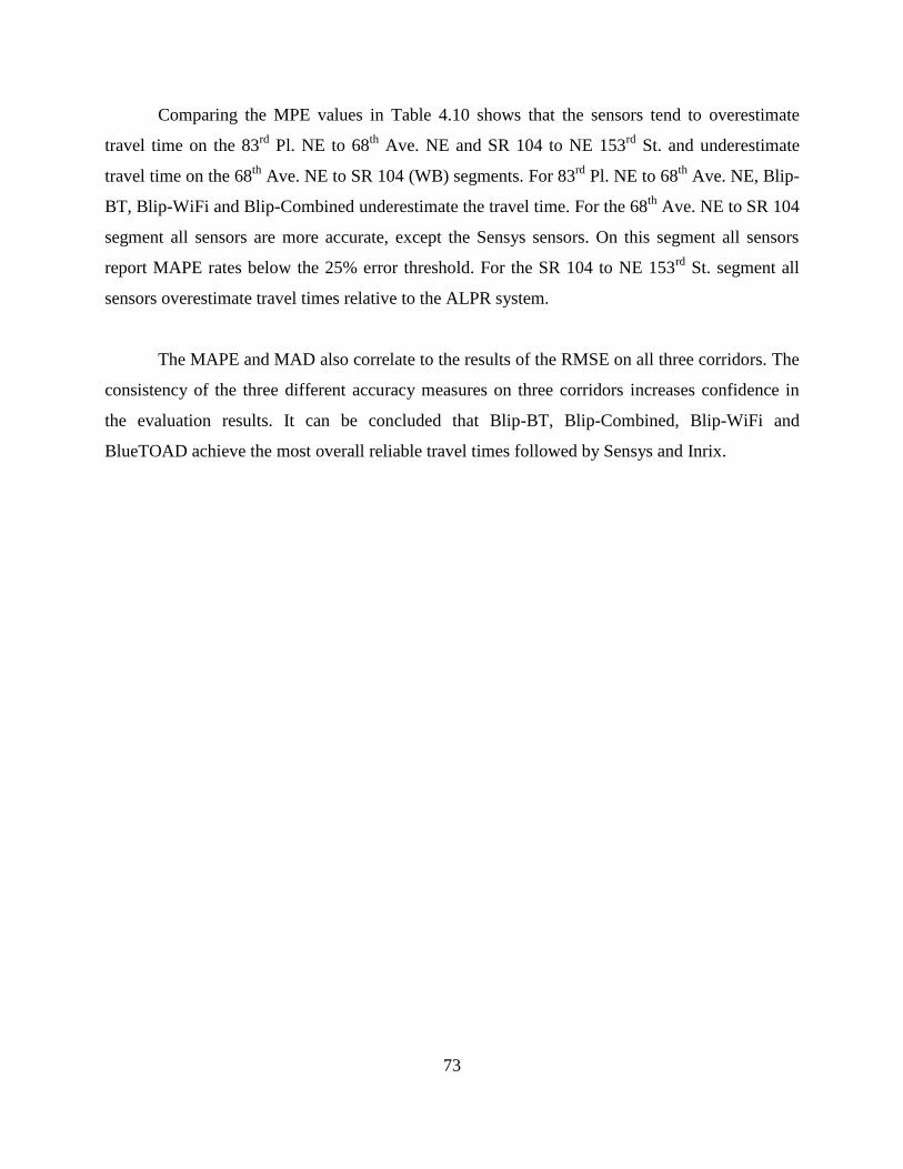
73

Comparing the MPE values in Table 4.10 shows that the sensors tend to overestimate

travel time on the 83rd

Pl. NE to 68th

Ave. NE and SR 104 to NE 153rd

St. and underestimate

travel time on the 68th

Ave. NE to SR 104 (WB) segments. For 83rd

Pl. NE to 68th

Ave. NE, Blip-

BT, Blip-WiFi and Blip-Combined underestimate the travel time. For the 68th

Ave. NE to SR 104

segment all sensors are more accurate, except the Sensys sensors. On this segment all sensors

report MAPE rates below the 25% error threshold. For the SR 104 to NE 153rd

St. segment all

sensors overestimate travel times relative to the ALPR system.

The MAPE and MAD also correlate to the results of the RMSE on all three corridors. The

consistency of the three different accuracy measures on three corridors increases confidence in

the evaluation results. It can be concluded that Blip-BT, Blip-Combined, Blip-WiFi and

BlueTOAD achieve the most overall reliable travel times followed by Sensys and Inrix.

74

Table 4.10 Travel time accuracy analysis for westbound SR 522 for the period of April 5th


,

2013

Note: The maximum accepted level of accuracy error is set as 25% for percent based error measures. The MAPE and

MPE are colored green below 15%, transitioning through yellow at 20% to red at or above 25%.

75

4.4.2 Eastbound Travel Time

Travel time plots for three segments on eastbound SR 522 are shown in Figure 4.17, Figure 4.18

through Figure 4.19 for the analysis period of May 1st, 2013 through May 8

th, 2013. The weekly

data demonstrates that the travel times on all three segments are consistent and cyclical. The

difference between weekdays and weekends is distinguishable. These results are in accordance

with expectations based on westbound performance.

The descriptive statistics for the two month period (April 5th


, 2013) are

summarized in Table 4.11. Due to the lack of ground truth on the eastbound segments it is not

possible to evaluate the sensors’ accuracy; however, it is clear the Inrix data indicates a

significantly higher or lower and more highly smoothed travel time over the off-peak hours

compared to the others. For the 68th

Ave. NE to 83rd

Pl. NE segment, the Inrix results are

significantly lower and less responsive than the other systems. For SR 104 to 68th

Ave. NE Inrix

reports a lower travel time, but with less separation than the other two segments and more

responsiveness to traffic conditions. For the NE 153rd

St. to SR 104 segment Inrix data is

generally higher and somewhat responsive to traffic conditions. Overnight, BlueTOAD was

observed to have a number of gaps in its data. This is not necessarily a problem, as it is likely an

effect of low traffic volumes, when travel time data is least likely to be needed, but the lack of

data should be noted.

In order to have an overall view of the accuracy of travel time estimation on eastbound, data

collected between 9 am and 10 am (an off-peak period) on Wednesdays across two months (April

5th


, 2013) are analyzed for all sensors. Table 4.11 presents descriptive

statistics of the collected data. As seen in Table 4.11 the average travel times are closely

estimated by all sensors. Inrix has the highest difference with the other sensors. The matches

recorded by Blip-BT, Blip-WiFi, Blip-Combined and BlueTOAD shown in Table 4.11 are

proportional to those shown in Table 4.8. This indicates that the penetration rate of each

individual system on both time scales and directions is consistent.

76

68th

Ave. NE to 83rd

Pl. NE (EB)

Figure 4.17 Travel time plot from 68th Ave. NE to 83rd Pl. NE (EB) for May 1st, 2013 through May 8th, 2013

Figure 4.17 shows the overlaid profiles of travel time for all the sensors on 68th

Ave. NE to 83rd

Pl. NE (EB) over the course of a week

from May 1st, 2013 through May 8

th, 2013. It is clear that all the sensors are capable of detecting the cyclical pattern of travel time over

weekdays and weekend and also for the morning and afternoon peaks. However, it is clear the Inrix reports a significantly lower and

highly smoothed travel time on this segment compared to others. Overnight, BlueTOAD was observed to have a number of gaps in its

data.

77

SR 104 to 68th

Ave. NE (EB)

Figure 4.18 Travel time plot from SR 104 to 68th Ave. NE (EB) for May 1st, 2013 through May 8th , 2013

Figure 4.18 shows the overlaid profiles of travel time for all the sensors on SR 104 to 68th

Ave. NE (EB) over the course of a week



weekdays and weekend and also for the morning and afternoon peaks. Overnight, BlueTOAD was again observed to have a number of

gaps in its data. The evening of May 2nd

, an incident caused a significant spike in travel times registered by all sensors.

Incident

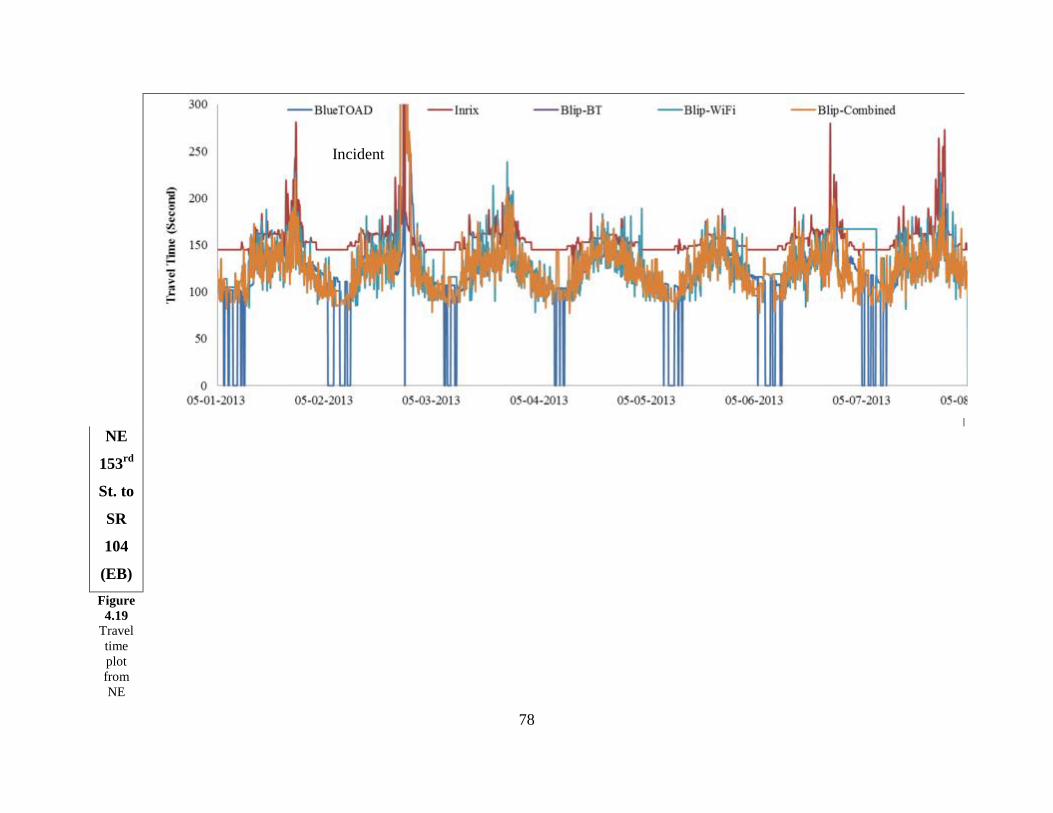
78

NE

153rd

St. to

SR

104

(EB)

Figure

4.19 Travel

time

plot

from

NE

Incident

79

153rd

St. to

SR

104

(EB)

for

May

1st,

2013

throug

h May

8th,

2013

Figure 4.19 shows the overlaid profiles of travel time for all the sensors from NE 153rd

St. to SR 104 (EB) over the course of a week



weekdays and weekend and also for the morning and afternoon peaks. Inrix reports a significantly higher and highly smoothed travel

time over the off-peak hours on this segment compared to others. Overnight, BlueTOAD was observed to have a number of gaps in its

data. The evening of May 2nd

, an incident caused a significant spike in travel times registered by all sensors.

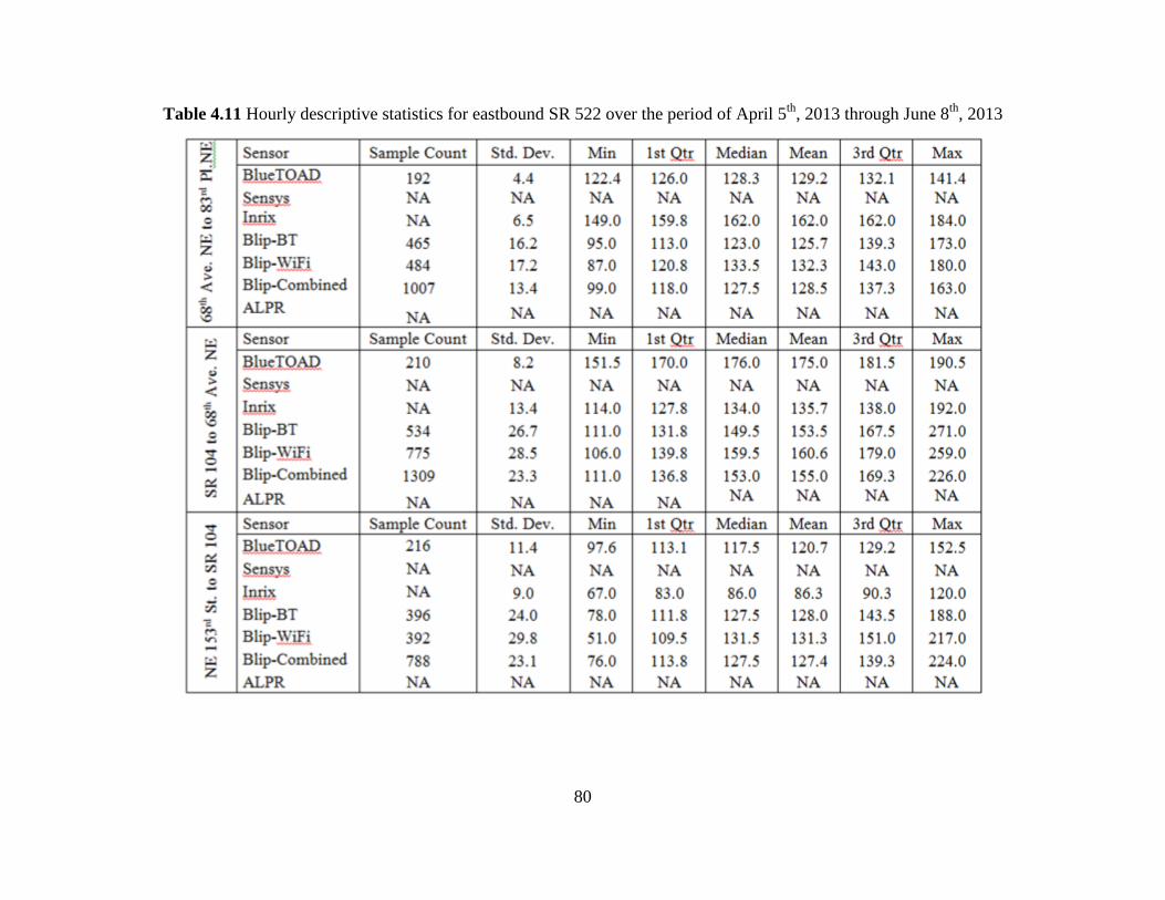
80

Table 4.11 Hourly descriptive statistics for eastbound SR 522 over the period of April 5th


, 2013

81

Table 4.11 presents the travel time samples recorded by each system grouped by segment

as well as the sample penetration rate compared to the ALPR system. The travel time standard

deviation in seconds, minimum travel time, 1st quartile, median, mean, 3rd quartile and max are

also presented.

4.5 Data Analysisfor I-90

The analysis of sensors placed on I-90 differs from the analysis of sensors installed on SR

522 in that there is not a system comparable to the ALPR system on SR 522 to use as a ground

truth travel time measurement. This restricts the analysis of I-90 data to be more qualitative than

the SR 522 analysis. Specifically, the evaluation of I-90 data looks at data availability, daily

pattern variation, and reaction to traffic events such as closures due to construction and snow

removal.

Figure 4.20, Figure 4.21, and Figure 4.22, show daily travel times for the westbound links


th, 2013. Note that I-90 from milepost 56 to 61 has been closed

occasionally for rock blasting related to construction. These closures are typically about an hour

in length and close both directions. The evening of May 2nd

, 2013 includes one such closure

which shows as a travel time peak in Figure 4.21. This event is shown more closely in Figure

4.23, and a similar closure on May 15th

, 2013 is shown in Figure 4.24.

Figure 4.23 and Figure 4.24 show how the Inrix and BlueTOAD data react to the absence

of traffic. The BlueTOAD system continues to report the last travel time for approximately a half

hour until ceasing to report travel times pending new vehicle identification. The Inrix data has a

more variable response. The Inrix travel time data is the sum of data from many smaller

segments. This factor is of limited impact on the SR-522 corridor due to smaller segment size and

fewer segments involved. For I-90, the longer distance between sensor placements means that

instead of one to three Inrix segments, ten to twenty may be involved. The difference in Inrix

response between Figure 4.23 and Figure 4.24 is that is that a number of segments reverted to

average travel time on May 15th

and on May 2nd

they reported null values instead.

82

However, other data produced by the systems are useful in identifying the closures. Inrix

reports a confidence level for its segment readings that can be used to judge the reliability of the

data. For both closures, the Inrix data reported significant decreases in average confidence and

complete absence of confidence for specific segments. The BlueTOAD data includes a useful

data point, the last reported matching vehicle. When the closure occurred, no more vehicles were

being detected to update the travel time information. After a half hour with no new samples the

BlueTOAD data ceased reporting a travel time.

It is important to note that calculating the travel time by averaging Inrix segment data is

very limited in the case of closures. This is because it is nearly impossible to accurately judge the

delay from being backed up and held at the closure site without some kind of arrival information.

This is a non-issue for BlueTOAD data, which presents a reasonable travel time, once traffic flow

has resumed, to judge by the travel times of approximately an hour reported after reopening the

road.

83

MP 109 to MP 70

Figure 4.20 Travel times on I-90 from Ellensburg (MP 109) to Easton (MP 70) for May 1st, 2013 through May 8

th, 2013

Figure 4.20 shows a comparison of the travel time generated by BlueTOAD and Inrix from milepost 109 to Milepost 70 on I-90. This

segment has relatively lighter traffic and therefore shows little day to day variation. Of note is a possible blocking incident on May 7.

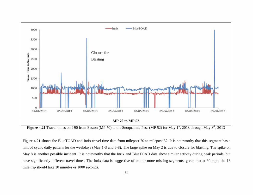
84

MP 70 to MP 52

Figure 4.21 Travel times on I-90 from Easton (MP 70) to the Snoqualmie Pass (MP 52) for May 1st, 2013 through May 8

th, 2013

Figure 4.21 shows the BlueTOAD and Inrix travel time data from milepost 70 to milepost 52. It is noteworthy that this segment has a

hint of cyclic daily pattern for the weekdays (May 1-3 and 6-8). The large spike on May 2 is due to closure for blasting. The spike on

May 8 is another possible incident. It is noteworthy that the Inrix and BlueTOAD data show similar activity during peak periods, but

have significantly different travel times. The Inrix data is suggestive of one or more missing segments, given that at 60 mph, the 18

mile trip should take 18 minutes or 1080 seconds.

Closure for

Blasting

85

MP 52 to MP 32

Figure 4.22 Travel times on I-90 from the summit (MP 52) to North Bend (MP 32) for May 1st, 2013 through May 8

th, 2013

Figure 4.22 shows the travel time data for Inrix and BlueTOAD from milepost 52 to milepost 32. This time it appears that BlueTOAD

is underestimating the travel time. The 20 mile segment should take 1200 seconds at 60 mph. Considering that this segment is

downhill from the Snoqualmie Pass summit it is reasonable to assume that speeds may be higher than expected by the speed limit.

However, the BlueTOAD travel time corresponds to a speed near 75 mph (which is quite possible on this section of I-90). There may

be differences in vehicle populations detected, with a bias towards commercial vehicles for Inrix and cars for BlueTOAD.

86

MP 70 to MP 52 Closure During Blasting May 2nd

, 2013

Figure 4.23 May 2nd

closure of I-90 and sensor response

Figure 4.23 shows a detailed view of the data for May 2nd

, 2013 on I-90. The vertical blue dotted lines indicate the start and end of the

closure. The blue triangles show the times of the last and first detected vehicles by BlueTOAD and the red dashed line indicates Inrix’s

average confidence value for the data. In this case the Inrix travel time responds immediately, but actually indicates a faster travel time

than during free flow. The BlueTOAD data shows a travel time for the segment for 30 minutes before ceasing to report data until

87

detecting the next vehicle. Of note is that the BlueTOAD data reflects a reasonable travel time upon resumption of traffic flow and

Inrix’s travel time quickly returns to normal.

MP 70 to MP 52 Closure During Blasting May 15th

, 2013

Figure 4.24 May 15th

closure of I-90 and sensor responses

Figure 4.24 shows a similar event on May 15th

, 2013. The vertical blue dotted lines indicate the start and end of the closure. The blue

triangles show the times of the last and first detected vehicles by BlueTOAD and the red dashed line indicates Inrix’s average

confidence value for the data. This time the Inrix data does not respond to the closure, but the confidence level drops dramatically

88

during the interval. Note that the confidence level shown in this figure is an average across multiple segments. Individual segments

have zero or near zero confidence during the closure.

89

4.6 Data Manipulation and Sensor Evaluation Conclusions

One of the major tasks of this project was collecting and manipulating the data from each

of the vendors. Each vendor uses different data formats, algorithms and frequently, technologies

making the task of collecting and organizing the data one that bears closer inspection. Collecting

and organizing data from an individual vendor is not an overly daunting task. Coordinating data

from four vendors and the WSDOT with seven distinct systems each generating multiple datasets

is a significant resource investment.

The major points of note in the data collection for this project are ease of data collection,

completeness of data, ease of mapping to existing data structures and consistency of availability.

Each vendor has a different means of distributing data, typically web based, though the WSDOT

ALPR and loop data and Inrix data came through email and network connections. The Sensys,

BlueTOAD and BlipTrack data all came through websites of differing utility.

Over the course of the project several changes were made to the vendor websites. Specific

issues encountered during the project were limitations in length of time, number of sensors and

speed of download. Initially, the Sensys website was a major limitation with small data download

limits requiring significant manual effort to collect all of the project data. The BlueTOAD and

BlipTrack websites were not as labor intensive but still required significant effort to collect and

collate all of the desired data.

Mapping the data collected to existing data structures; in this case, the data and sensor

placement of the ALPR system on SR 522 and the milepost/exit pattern for I-90 was trivial in

some cases and more difficult in others. For SR 522 WB, the sensor sites were chosen to match

existing westbound ALPR locations, making the matchup between each set of data easy.

Eastbound SR 522 has a different ALPR setup in that there is no ALPR at the SR-104

intersection for eastbound traffic. The nearest ALPR for eastbound traffic is located 0.2 miles

west at the Beach Drive NE intersection. This makes a direct mapping of sensors to eastbound

90

ALPR data impossible. Incidentally, the ALPR data for eastbound experienced a data collection

failure during the analysis period, precluding an analysis in any case.

Inrix data has been the major source of issues mapping data to existing data structures.

Inrix data is keyed to a different base mapping system than the other systems and the ALPR data.

Inrix data uses TMC codes to identify roadway segments in a system developed for GPS systems

instead of the route and milepost or arbitrary sensor number/placement data systems used by the

other systems. Where Inrix TMC segments do not exactly map to existing segments; its travel

time will be over or underestimated compared to the other systems as seen in the SR 522 analysis

in particular. Another consequence of this difference in mapping is that an analysis segment

composed of more than one Inrix TMC segments will need to reconcile potentially very different

travel times on an individual TMC segment and normal travel times on others. Specifically, this

occurs when delay or stoppage is incurred. For example at an intersection or blockage on a

freeway, an individual TMC segment may report a high travel time (even exceeding the 5 minute

reporting interval) while the surrounding TMC segments report normal travel times. The sum of

travel time across TMC segments used in this research fails when significant stoppage or delay

occurs, because the sum of travel time across the relevant TMC segments will include free

flowing segments beyond the blockage as seen in the I-90 data analysis.

An additional point of interest that falls under data mapping is the inclusion of different

data collected by each system and different smoothing algorithms. Each system includes time and

travel time information in its basic data formats. BlueTOAD data includes its match rates in a

separate file system at 15 minute time intervals instead of the 5 minute intervals used for the

other data. Inrix data does not include a capture rate as such, but does have a confidence value as

shown in the I-90 analysis. The remaining systems report their matches and travel times in the

same files and data structures. The Sensys system has the most additional data associated with it.

Specifically Sensys includes travel time measurements at 10% intervals, measured speeds and

upstream and downstream volumes. For this research the 90% travel time was chosen to represent

the Sensys travel time, as that was the value used by Sensys to represent travel times in their

presentation to the lab. This is a conservative measure that can underestimate the accuracy of the

91

Sensys system. It should be noted that even with this potential handicap, the Sensys system

proved to have acceptable levels of accuracy in several cases.

Data availability is a multifaceted problem. First, the data must be collected by the system

in question. This includes all of the communications and storage endemic to collecting the data.

The second aspect is that the data must be retrievable by the system. Finally, there are temporal

availability considerations. These include considerations of delay between collection and

accessibility of the data and how long the data is available after collection. In this project,

immediate temporal availability has not been of primary concern, however it should be noted that

the data delivery methods for data from the WSDOT and Inrix included delays between

collection and availability.

To help readers get a better feel for the behavior of the various systems and to disseminate

data the research team has developed a webpage as part of the Digital Roadway Interactive

Visualization and Evaluation Network (DRIVE Net). DRIVE Net is a University of Washington

Smart Transportation Applications and Research Lab (STAR Lab) data management and analysis

tool developed to showcase research results. Figure 4.25 and Figure 4.26 show the I-90 and SR

522 data analysis interfaces. The webpage may be accessed at sensors.uwdrive.net.

http://www.sensors.uwdrive.net/

92

Figure 4.25 I-90 data analysis interface for sensors.uwdrive.net

Figure 4.26 SR 522 data analysis interface for sensors.uwdrive.net

94

Chapter 5 Summary of the results and discussions

Note that high level conclusions are presented here. For detailed observations see the

relevant chapters. Readers are encouraged to review Figure 1.1, Figure 4.1, Figure 4.9, Figure

4.10 and Figure 4.24 specifically. Also, remember that the relationship between accuracy of the

information obtained by ATIS and the benefits for the users was determined for a case study in

Los Angeles (see Figure 1.1 ). The researchers found that when accuracy drops below a critical

point, users are better off not using the data provided by the ATIS and relying instead on

experience with historical traffic patterns. One of the goals of this research was to provide

decision makers with sufficient information to select an appropriate system for the corridor in

question.

Travel time information is a valuable commodity for ITS and operations. Road users

benefit from accurate travel time information that allows them to plan their trips. Accurate travel

time information will also allow road users to avoid congestion and incidents, potentially

reducing the severity of congestion caused by incidents and recurring congestion. Engineers can

use travel time data to analyze the effectiveness of various changes to corridor operations, such as

signal retiming and geometric changes.

This study focuses on two test corridors. The first test corridor is State Route 522 between

the NE 153rd

Street and 83rd

Place NE intersections. This section of SR 522 is an urban arterial

with frequent intersections. This corridor experiences heavy daily commuting traffic and has

frequent incidents that can make travel times unpredictable. An automated license plate reader

system has been in place on the SR 522 corridor for a number of years with three westbound

segments in the study area, from 83rd

Pl. NE to 68th

Ave. NE, 68th

Ave. NE to SR 104 and SR

104 to NE 153rd

St. For this analysis, even though the ALPR system has different segments on

eastbound SR 522, the analysis used the same segments for eastbound because every other

system used the same segments eastbound and westbound.

95

The second test corridor is on I-90 from milepost 109 (Ellensburg, WA) to milepost 32

(North Bend, WA). This section of I-90 is a rural freeway from western Washington to eastern

Washington over the Snoqualmie Pass whose summit is at milepost 52. There were no pre-

existing travel time measurement systems on I-90 before this study. Segments on I-90 are

described by mileposts 32, 52, 70 and 109.

The sensor systems deployed on SR 522 include the pre-existing ALPR system, a Sensys

emplacement on westbound SR 522, the TrafficCast BlueTOAD system, Blip Systems BlipTrack

sensors and a 3rd

party feed from Inrix. The I-90 corridor was instrumented with the BlueTOAD

system in addition to using the Inrix data feed. The ALPR system reads the license plates of

vehicles passing the sensors and holds the license plate number in memory until the vehicle

passes the next sensor location. The Bluetooth and WiFi sensors built into the BlueTOAD and

BlipTrack systems function similarly by reading the MAC address of wireless electronic devices

from location to location. The Sensys system reads the magnetic signature of passing vehicles

and attempts to match vehicles based on signature and platoon organization. The Inrix data is

based on cellphone and GPS data from its users.

Collecting the data for this project has been a significant expenditure of effort. Collecting

data from the WSDOT, Inrix, Sensys, TrafficCast, and Blip Systems has required the research

team to visit multiple websites and databases. Collating and organizing data with different

temporal resolutions, included data and segments required the research team to find common

intervals and expend significant effort just to make the different data sets comparable.

There are two important factors to consider in analyzing the sensor results. The first is the

accuracy of the reported travel time. To address this each sensors’ data is compared against the

ALPR system on westbound SR 522. The ALPR system has been previously evaluated and

deemed accurate enough to serve as the ground truth for this study. The lack of ALPR data or

other similarly dependable travel time data source limits the research team’s ability to analyze

eastbound SR 522 and the I-90 corridor. A number of accuracy measures have chosen for this

analysis to give readers more insight into the frequency, severity and directionality of errors.

96

The westbound SR 522 analysis found that the accuracy of the systems varied by segment

with every system reporting their least accurate travel times on the 83rd

Pl. NE to 68th

Ave.NE

segment. The daily analysis revealed that the systems experienced error spikes during the

morning peak period on all segments. With the exception of the Inrix data, all systems generally

reported satisfactory results, with the Bluetooth and WiFi based systems staying below the 25%

error threshold except during overnight hours and some spikes in the peak periods. It should be

noted that the Sensys travel time used was the 90th

percentile travel time, where the other systems

reported mean or median values, yet still the Sensys system posted acceptable accuracy in most

cases. The Sensys travel time error may be reduced by selecting another one of the ten provided

travel time values.

The systems did have some notable accuracy limitations. Specifically, the BlueTOAD

system can be less reliable overnight when sampling is low. The Inrix system was generally the

least responsive to traffic changes and tended to have systematically high or low travel times,

probably the results of conservative free flow travel time estimation.

The I-90 and eastbound SR 522 analysis of travel time focused on more qualitative

aspects of system performance. For I-90, the research team was looking for reasonable travel

times and daily traffic patterns as well as response to known road closure events. The eastbound

SR 522 results met expectations based on the westbound analysis, with most patterns repeating,

including the systematic over or underestimation of travel time by Inrix. The I-90 analysis noted

that both systems were able to respond to daily patterns; however, Inrix and BlueTOAD reported

significantly different results on some segments. When the road closure time periods were

examined, both systems had their flaws. The BlueTOAD system continued to report a travel time

for 30 minutes after the road closure and the Inrix data either failed to react significantly to the

closure or reported impossible travel times. Both systems include specific data that can be used to

identify when such event occur.

The second important factor to consider in the sensor analysis is the sample size used to

calculate the travel time. If the sample size is too small, the travel time may not be representative.

Sample size is affected by several factors, including traffic volume and mobile device penetration

97

rates (for Bluetooth and WiFi sensors). For westbound SR 522 the ALPR and Sensys systems

have comparable absolute detection rates with between 25% and 50% of traffic being detected,

depending on time of day and location. The Bluetooth and WiFi systems detect significantly

fewer vehicles. BlueTOAD captured about 6% of the volume captured by the ALPR system for

an absolute capture rate near 2% of total traffic The BlipTrack system captured roughly double

the number of Bluetooth readings and two and a half times as many on WiFi. The BlipTrack

sensor also reports combined totals for its Bluetooth and WiFi sensors, which pushes the combine

BlipTrack system to approximately 25% of the ALPR capture rate. Because of the nature of the

Inrix data, there is no capture rate to analyze.

The collection of sensors assembled for this study is impressive. By setting up so many

sensors on the same corridor and having reliable ground truth data in the form of an established

ALPR system, the WSDOT has made it possible to perform an in-depth analysis of the different

systems. This work shows that sensors of different types and complexities can accomplish the

goal of measuring travel time.

Ultimately, each system in the analysis has different strengths and weaknesses that should

be considered in addition to their accuracy and sample rates. Some systems can provide

additional data; others trade accuracy and coverage for cost or portability. Ultimately, engineers

will need to weigh their requirements for accuracy and sample rates against the other engineering

constraints imposed on their system. For example, the BlueTOAD units installed on SR 522 and

I-90 are solar powered and use cellular data networks, reducing infrastructure and deployment

costs. The BlipTrack units have higher sampling rates and marginal accuracy superiority in

exchange for power requirements. The Inrix data does not require any DOT infrastructure and has

wide availability. ALPR units have high accuracy and a comparatively high installation cost. The

Sensys system has perhaps the most complicated set of tradeoffs. Sensys magnetometers can be

used as replacements for loop detectors in intersection operations, making the marginal costs of

adding Sensys re-identification lower at some intersections than others.

98

References

Ahmed, H., M. El-Darieby, B. Abdulhai, and Y. Morgan. Bluetooth- and Wi-Fi-Based

Mesh Network Platform for Traffic Monitoring. In Transportation Research Board 87th

Annual Meeting. CD-ROM. Transportation Research Board, 2008.

Blip Systems. BlipTrack collecting real-time travel information. Available from:

http://media.brintex.com/Occurrence/27/Brochure/1279/brochure.pdf [Accessed 15th

November 2013].

Blip Systems. BlipTrack Wi-Fi Traffic Sensor. Available from:

http://www.blipsystems.com/traffic/products/bliptrack-wi-fi-traffic-sensor/ [Accessed 15th

November 2013].

Bullock, D., R. Haseman, J. Wasson and R. Spitler. “Anonymous Bluetooth Probes for

Measuring Airport Security Screening Passage Time: The Indianapolis Pilot Deployment”

In Transportation Research Board 89th Annual Meeting. CD-ROM. Transportation

Research Board, Washington D.C., 2010.Eberle Design Inc. Oracle 2EC. Available from:

http://www.editraffic.com/wp-content/uploads/Oracle_2EC_4EC_Catalog_Sheet.pdf

[Accessed 15th November 2013].

Gramaglia, M., Bernardos, C.J., Calderon, M. Virtual induction loops based on cooperative

vehicular communications. Sensors 2013, 13, 1467–1476.

Haghani, A., M. Hamedi, K.F. Sadabadi, S. Yound Young and P. J. Tarnoff. “Freeway

Travel Time Ground Truth Data Collection Using Bluetooth Sensors.” Transportation

Research Record: Journal of the Transportation Research Board, 2010.

Jung, S. J. Larkin, V. Shah, A. Toppen, M. Vasudevan and K. Wunderlich (2003). On-time

Reliability Impacts of ATIS, Volume III: Implications for ATIS Investment Strategies.

Final Report. 85 p. + app. 14 p.

http://media.brintex.com/Occurrence/27/Brochure/1279/brochure.pdf

http://www.blipsystems.com/traffic/products/bliptrack-wi-fi-traffic-sensor/

http://www.editraffic.com/wp-content/uploads/Oracle_2EC_4EC_Catalog_Sheet.pdf

99

Chen, LJ and HH Hung, "A Two-State Markov-based Wireless Error Model for Bluetooth

Networks," Wireless Personal Communications Journal, Springer, volume 58, number 4,

pages 657-668, June 2011.

Haseman, R.J., J. Wasson and D. Bullock. “Work Zone Travel Time Delay and Evaluation

Metrics Using Bluetooth Probe Tracking” In Transportation Research Board 89th Annual

Meeting. CD-ROM. Transportation Research Board, Washington D.C., 2010.

Hewlett Packard. Wi-Fi and Bluetooth interference issues. 2002.

Huang, A.S. and L. Rudolph. (2007). Bluetooth essentials for programmers, Cambridge

University Press, New York, NY., 2007.

Inrix. Available from: http://www.inrix.com/. [Accessed 15th

November 2013].

Lighthill, M.J. and G.B. Whitham (1955) on Kinematic Waves. A theory of traffic flow on

long crowded roads. Proc R Soc London Ser A 229:317–345.

Ma, X., Y.J. Wu, and Y. Wang. DRIVE Net: An E-Science of Transportation Platform for

Data Sharing, Visualization, Modeling, and Analysis. Paper 11-4106 for the 90th Annual

Meeting Transportation Research Board, Washington, D.C., 2011.

Mathe, T. V. (2013) Travel Time Data Collection, Available from:

http://www.civil.iitb.ac.in/~vmtom/1111_nptel/527_AutoGPS/plain/plain.html [Accessed:

November 14th 2013].

Meehan, B. (2005). Transportation Information Management Team, Federal Highway

Administration. Travel Times on Dynamic Message Signs. Travel Time Messages on

Dynamic Message Signs National Transportation Operations Center (NTOC) Web Casts

Archive. Available from: http://www.ntoctalks.com/web_casts_archive.php.

Mizuta, K., Automated License Plate Readers Applied to Real-Time Arterial Performance:

A Feasibility Study, Department of Civil & Environmental Engineering: University of

Washington, 2007.

http://www.inrix.com/

http://www.civil.iitb.ac.in/~vmtom/1111_nptel/527_AutoGPS/plain/plain.html

http://www.ntoctalks.com/web_casts_archive.php

100

Monsere, C., A. Breakstone, R. L. Bertini, D. Deeter, and G. McGill. “Validating Dynamic

Message Sign Freeway Travel Times Using Ground Truth Geospatial Data. In

Transportation Research Record: Journal of the Transportation Research Board, No. 1959,

TRB, National Research Council, Washington, D.C., 2006, pp. 19–27.

Paniati, F. J., “Dynamic Message Sign Recommended Practice and Guidance”. FHWA

Memorandum, July 16, 2004. Available from: http://mutcd.fhwa.dot.gov/res-

memorandum_dms.htm [Accessed 10th October 2010].

PIPS Technology. Product Overview. Available from: http://www.ae-

traffic.com/NuMetrics/AE_Traffic_ALPR.pdf [Accessed 15th

November 2013].

Pokrajac, D., C. Borcean, A. Johnson, A. Hobbs, L. Agodio, S. Nieves, M. Balbes, L.

McCauley, J. Tice, N. Dare, J. McKie, B. Lombardo, B.J. Self, and J. Austin, "Evaluation

of automated license plate reader accuracy," 9th International Conference on

Telecommunication in Modern Satellite, Cable, and Broadcasting Services, 2009, vol., no.,

pp.217-220, 7-9 Oct. 2009.

Quayle, S., P. Koonce, D. DePencier, and D. Bullock. “Freeway Arterial Performance

Measures Using MAC Readers: Portland Pilot Study” In Transportation Research Board

89th Annual Meeting. CD-ROM. Transportation Research Board, Washington D.C., 2010.

Rakha, H. and W. Zhang, Estimating traffic stream space-mean speed and reliability from

dual and single loop detectors. Transportation Research Record, 1925 (2005), pp. 38–47.

RENO A&E. Model C-1000 Series. Available from:

http://www.signalcontrol.com/products/reno/RenoAE_C_Series_Rack_Mount_LCD_Det.p

df [Accessed 15th November 2013].

Innamaa, S. (2009). Short-term prediction of traffic flow status for online driver

information. VTT Publications, 708.

http://mutcd.fhwa.dot.gov/res-memorandum_dms.htm

http://mutcd.fhwa.dot.gov/res-memorandum_dms.htm

http://www.ae-traffic.com/NuMetrics/AE_Traffic_ALPR.pdf

http://www.ae-traffic.com/NuMetrics/AE_Traffic_ALPR.pdf

http://www.sciencedirect.com/science/article/pii/S0968090X10000604#bib19

http://www.signalcontrol.com/products/reno/RenoAE_C_Series_Rack_Mount_LCD_Det.pdf

http://www.signalcontrol.com/products/reno/RenoAE_C_Series_Rack_Mount_LCD_Det.pdf

101

Sensys Networks, VSN240 Wireless Flush-Mount Sensor. Available from:

http://www.sensysnetworks.com/downloads/data-sheets/Datasheet-VSN240-Sensor.pdf

[Accessed 15th November 2013].

Sreedevi, I. 2005 ITS decision services and technologies loop detectors. Available from:

http://www.calccit.org/itsdecision/serv and tech/Traffic Surveillance/road-based/in-

road/loop summary.html [Accessed 15th

November 2013].

Special Interests Group (SIG). Core Specification v4.0, June, 30, 2010.

www.bluetooth.com

Tarnoff, P.B., Darcy; Young, Stanley; Wasson, James; Ganig, Nicholas; Sturdevant, James.

Continuing Evolution of Travel Time Data Information Collection and Processing In

Transportation Research Board 88th Annual Meeting. CD-ROM. Transportation Research

Board, Washington D.C., 2009.

Toppen A & Wunderlich K 2003. Travel time data collection for measurement of advanced

Traveler information systems accuracy. Federal Highway Administration, Project No.

0900610-D1. 20 p.

TraffiCast. Bluetooth™ detection for Travel Times & Road Speeds. Available from:

http://trafficcast.com/products/view/blue-toad/ [Accessed 15th November 2013]

Traficon. VIP3D.1 & VIP3D.2 Vehicle Presence & Data Detector. The Original 170,

NEMA TS-1 & TS-2 Plug-In Module, 2nd Generation. Available from:

http://www.kargor.com/CL_VIP3D_USAsize_Sep08_email.pdf [Accessed 15th November

2013].

Turner, S. M., W. L. Eisele, R. J. Benz, and D. J. Holdene, Travel Time Data Collection

Handbook, Federal Highway Administration, U.S. Department of Transportation and

Texas Transportation Institute, Texas A&M University System, CD-ROM (FHWA-PL-98-

035), March 1998.

http://www.sensysnetworks.com/downloads/data-sheets/Datasheet-VSN240-Sensor.pdf

http://www.calccit.org/itsdecision/serv%20and%20tech/Traffic%20Surveillance/road-based/in-%20road/loop%20summary.html

http://www.calccit.org/itsdecision/serv%20and%20tech/Traffic%20Surveillance/road-based/in-%20road/loop%20summary.html

http://trafficcast.com/products/view/blue-toad/

http://www.kargor.com/CL_VIP3D_USAsize_Sep08_email.pdf

102

Washington State Office of Financial Management. "Rank of Cities and Towns by April 1,

2009 Population Size" April, 2009. http://www.ofm.wa.gov/pop/april1/rank2009.pdf.

Retrieved November 29th

, 2009.

Wasson, J.S., J.R. Sturdevant, and D.M. Bullock. Real-Time Travel Time Estimates Using

Media Access Control Address Matching. ITE Journal, Vol. 78, No. 6, 2008, pp. 20-23.

Weiss, T. and E. Schmitt. Where The Jobs Are, Spring 2009. Forbes.com. March 10, 2009.

Retrieved February 28, 2010.

http://www.ofm.wa.gov/pop/april1/rank2009.pdf



http://www.forbes.com/2009/03/09/cities-jobs-spring-leadership-careers-best.html

103

Appendix A: SR 522 and I-90 Corridor Details

I-90 Study Route

Site A, Milepost 32, North Bend, WA (BlueTOAD Circled)

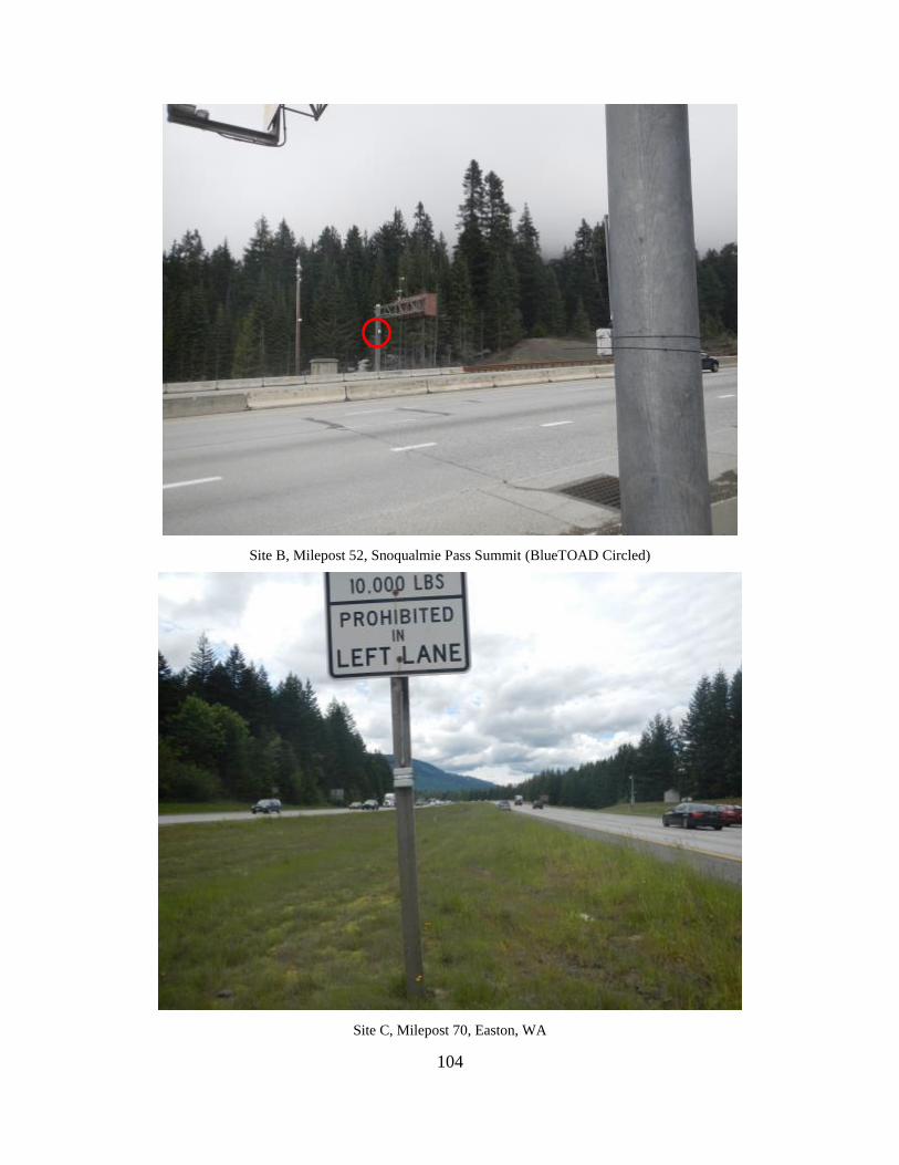
104

Site B, Milepost 52, Snoqualmie Pass Summit (BlueTOAD Circled)

Site C, Milepost 70, Easton, WA

105

Site D, Milepost 109, Ellensburg, WA (BlueTOAD Circled)

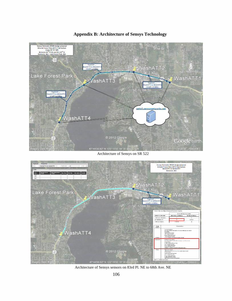
106

Appendix B: Architecture of Sensys Technology

Architecture of Sensys on SR 522

Architecture of Sensys sensors on 83rd Pl. NE to 68th Ave. NE

107

Architecture of Sensys sensors on 68th Ave. NE to SR 104

Architecture of Sensys sensors on SR 104 to NE 153rd St.

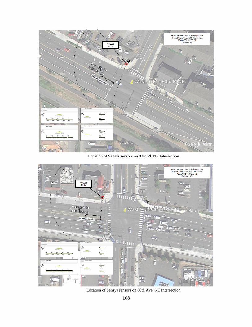
108

Location of Sensys sensors on 83rd Pl. NE Intersection

Location of Sensys sensors on 68th Ave. NE Intersection

109

Location of Sensys sensors on SR 104 Intersection

Location of Sensys sensors on 153rd St. Intersection

ERROR ASSESSMENT FOR EMERGING TRAFFIC DATA...

Documents

Transcript of ERROR ASSESSMENT FOR EMERGING TRAFFIC DATA...