Ergodic Theory - Paul Carlisle Kettler

Ergodic Theory

Paul C. Kettler, ’63

Thesis Submitted in Partial Fulfillmentof the Requirements

for the Bachelor of Arts Degree

Department of MathematicsPrinceton University

1963

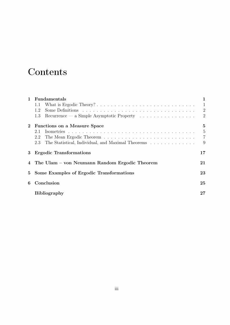
Contents

1 Fundamentals 11.1 What is Ergodic Theory? . . . . . . . . . . . . . . . . . . . . . . . . . . . . 11.2 Some Definitions . . . . . . . . . . . . . . . . . . . . . . . . . . . . . . . . 21.3 Recurrence — a Simple Asymptotic Property . . . . . . . . . . . . . . . . 2

2 Functions on a Measure Space 52.1 Isometries . . . . . . . . . . . . . . . . . . . . . . . . . . . . . . . . . . . . 52.2 The Mean Ergodic Theorem . . . . . . . . . . . . . . . . . . . . . . . . . . 72.3 The Statistical, Individual, and Maximal Theorems . . . . . . . . . . . . . 9

3 Ergodic Transformations 17

4 The Ulam – von Neumann Random Ergodic Theorem 21

5 Some Examples of Ergodic Transformations 23

6 Conclusion 25

Bibliography 27

iii

iv CONTENTS

Chapter 1

Fundamentals

1.1 What is Ergodic Theory?

Briefly, ergodic theory is the study of the asymptotic behavior of certain classes of measure-preserving transformations from a measure space to itself. Unfortunately, such a simpledefinition gives little insight toward justifying any special interest in the subject. Tounderstand why mathematicians began to develop the theory it is necessary to look intothe subject’s history.

Ergodic theory has its origins in statistical mechanics. Physicists discovered that thestate of a contained gas, for example, could be described by giving the location of eachparticle along with its velocity. Thus in the case of n particles, the state of the system couldbe specified by giving 6n numbers, or coordinates — three position components and threevelocity components — for each particle. Such a 6n-tuple was considered to be a pointin a 6n-dimensional “phase” space. Assuming that phase space were assigned a metric,and that the states varied continuously with time, a continuous curve was described inthe phase space. According to classical mechanics, the knowledge of one point on thiscurve would enable one to determine in theory the path of the curve as time continued.In practice, however, it is not possible to determine so accurately the state of a system.Hence, a more relevant question than, “Given the state at time t0, what will the state beat time t1?” is the question, “Given that the state at time t0 lies in a subset U of phasespace, what is the probability that at time t1 the state lies in subset V of phase space?”An even more interesting question is, “What will probably happen to the points of U as ttends to infinity?”

Such considerations led Liouville to investigate what happens to a subset of phase spacewhen the space changes (flows) continuously with time according to accepted physical laws.An important theorem of his in statistical mechanics states that if phase space is assignedthe Euclidean metric, then the Lebesgue measure of a subset equals the Lebesgue measureof its transform.

To the mathematician a number of theoretical questions arose immediately. One ofthese was, “What can be said concerning Liouville’s theorem if the number of particles is

1

2 CHAPTER 1. FUNDAMENTALS

taken to be infinite, or if the containing space is many dimensional or infinite dimensional?”Another was, “What happens if the transformations of a space are arbitrary, and notrestricted to one-parameter groups of transformations such as phase space flows?” Withthese questions before them, the mathematicians took their basic space to be an abstractspace with a measure assigned, took their transformations to be simple functions from thespace to itself, and with appropriate simplifications as necessary for convenience began toexamine the properties of measure-preserving transformations as applied repeatedly to thebasic space.

This disquisition owes undying gratitude to the seminal contributions of pioneers ofthis and related fields, as represented particularly in these works which are otherwise notcited, but whose influence pervades the entire book (Kakutani 1950; Riesz and Sz.-Nagy1955; Halmos 1956; Kolmogorov and Fomin 1961).

1.2 Some DefinitionsBefore plunging directly into the theory it is necessary to be familiar with the severalconcepts defined below.

Definition 1.1. A sigma-algebra of sets is a collection of sets that is closed under countableunions, intersections, symmetric differences, complements, and combinations thereof. Inparticular, the union of all the sets is an element in the algebra.

Definition 1.2. A measure is a non-negative, countably additive set function.

Definition 1.3. A measure space is a sigma-algebra of sets, together with a measuredefined on all elements of the algebra.

Definition 1.4. A sigma-finite measure space is a measure space with the restriction thatthe entire space is the union of countably many sets of finite measure. We will consideronly sigma-finite measure spaces.

Definition 1.5. A measurable transformation is a function from a space to a measurespace such that the inverse image of a measurable set is a measurable set.

Definition 1.6. A transformation T mapping a measure space X onto a measure spaceY is called invertible if there exists a transformation S such that ST (x) = x for all x inX. It follows that TS(y) = y for all y in Y , and we are therefore justified in calling S theinverse of T , written T−1.

1.3 Recurrence —a Simple Asymptotic Property

For a measure-preserving transformation from a measure space of finite measure to itselfa general theorem regarding the recurrence of points under repeated application of thetransformation can be stated.

1.3. RECURRENCE — A SIMPLE ASYMPTOTIC PROPERTY 3

Theorem 1.7. If U is a measurable subset of a space X of positive measure, and Tis a measure-preserving transformation from X to itself, then for almost every x ∈ U ,Y n(x) ∈ U for some n.

Proof. The proof is indirect. Look at the set of points U ′ ⊂ U such that for any x′ ∈ U ′,T n(x′) /∈ U for any n. Following from the fact that the transform of any point in X is eitherin U or in X \ U , we know that U ′ is always measurable. Explicitly, it is the countableintersection of measurable sets given by

U ′ = U ∩ T−1(X \ U) ∩ T−2(X \ U) ∩ · · · ∩ T−n(X \ U) ∩ · · · ,

where T−n(X \U) means the set of points mapped into X \U by T n, etc. Assume that themeasure of U ′ is positive. From the construction of U ′, T−n(U ′) is disjoint from U ′ for alln, for if that were not the case then there would be a point in U ′ such that its transformunder T n were also in U ′, contradicting the assumption. Furthermore, the whole sequence{T n(U ′)} is mutually disjoint, because

T−(n+k)(x) ∈ U ′ ⇐⇒ T−n(x) ∈ T−k(U ′),

implying that

T−n(U ′) ∩ T−(n+k)(U ′) = T−n(U ′ ∩ T−k(U ′)

),

which is empty. Inasmuch as T is measure preserving and the measure of X is finite, acontradiction has been established.

Theorem (1.7) can actually be strengthened by replacing “some n” by “infinitely manyn.”

Theorem 1.8. Given the hypothesis of Theorem (1.7), for almost every x ∈ U , T n(x) ∈ Ufor infinitely many n.

Proof. Let Un be the set of points which never return to U under repeated applications ofT n, and let V be the set of all x such that x ∈ U \ (U1∪U2∪· · · ). Since x ∈ U \U1, TN(x)is in U for some N . Since x ∈ U \ UN , TMN(x) ∈ U for some M . The argument can becontinued indefinitely, giving an infinite sequence of recurrence times.

4 CHAPTER 1. FUNDAMENTALS

Chapter 2

Functions on a Measure Space

2.1 Isometries

Given a measure space X and a measure subspace U , define a characteristic functionf : X 7→ R as follows. Let

f(x) =

{1 for x ∈ U

0 for x ∈ X \ U

Then using this definition, Theorem (1.8) could be restated, “Given the hypothesis ofTheorem (1.7), for almost every x ∈ U , the series {Sn}, where Sn =

∑n−1i=0 f

(T i(x)

),

diverges.” At this point, an important generalization can be made. We need not restrictconsideration to the characteristic function. Any non-negative, measurable function willwork as well. Recall:

Definition 2.1. a measurable function from a measure space to the complex numbers isa function constructed so that the set of points {x} such that |f(x)| < r is a measurableset for any real r. Then we have:

Theorem 2.2. Given a measure space X and a non-negative (real-valued) measurablefunction f, then for almost every x ∈ U , where U is the set of all x with f(x) ≥ 0, thesequence {Sn}, where Sn =

∑n−1i=0 f(T i)(x), diverges.

Proof. Let Uj be the set of all x such that f(x) ≥ 1/j. Then ∪∞j=1Uj = U , and byTheorem (1.8) almost every x ∈ Uj returns to Uj infinitely often. For every x ∈ U we canpick a j so that x is in Uj. For almost every x in this Uj the number of terms of {Sn}greater than 1/j increases without bound as n goes to infinity. Since no term of {Sn} isnegative, {Sn} diverges. The conclusion follows from the fact that the set of points forwhich {Sn} possibly does not diverge has measure zero in each Uj, and U is a countableunion of the {Uj}.

Knowing that almost every point of a subspace U of a measure space X returns toU infinitely often under the repeated applications of a measure-preserving transformation

5

6 CHAPTER 2. FUNCTIONS ON A MEASURE SPACE

T leads one to consider the following question: “As n gets large, for what fraction of thespaces T i(U), 0 ≤ i ≤ n− 1, is the point T i(x) contained in T i(U), x ∈ U? Furthermore,does this fraction tend to a limit as n goes to infinity?” If we again define a characteristicfunction f on X such that f on points of U is 1 and f on other points of X is 0, the fractionunder consideration is (1/n)

∑n−1i=1 f

(T i(x)

). Actually, with the problem in this state the

analysis involves the tricky problems of pointwise convergence, left for later. At this stage,it is more instructive to examine first certain relationships among functions of X. Supposewe begin to consider not just real-valued functions, but complex-valued functions, also,and suppose we define g(x) equal to f

(T (x)

). Then knowing f gives us g, i.e., g can

be written as a function of f , say R(f). Then if we let h(x) = g(T (x)

)= f

[T

(T (x)

)],

written f(T 2(x)

), we have h = R(g) = R

(R(f)

), written R2(f). Continuing the process

inductively, we see that T i corresponds, in the above manner, to Ri for all positive i. Wefind, then, that the transformation R has some familiar properties. First of all it is linear.Given complex numbers a and b, R(af + bg) = aR(f) + bR(g). This fact follows directlyfrom the definition of R.

R(af + bg)(x) = (af + bg)(T (x)

)= af

(T (x)

)+ bg

(T (x)

)= aR(f)(x) + bR(g)(x),

for all x. Furthermore, we have an important theorem regarding the action of R on acertain space of functions. Before giving the theorem, I list the following definitions.

Definition 2.3. The space of complex-valued functions on a measure space X such that(∫X|f(x)|k dµ

)1/k

is finite is called the Lk space, for positive integral k. (µ is the measuredefined on the measure space.)

Definition 2.4. The Lk norm of a function in the Lk space is the quantity(∫X|f(x)|k dµ

)1/k

, written ‖f‖k.

Definition 2.5. An isometry on the Lk space is a transformation S such that for f ∈ Lk,also Sf ∈ Lk, and ‖Sf‖k = ‖f‖k.

Theorem 2.6. Given a measure-preserving transformation T on a measure space X, thefunction R defined by Rf(x) = f

(T (x)

)for all x ∈ X is an isometry on L1.

Proof. Take the characteristic function g of a subset U of finite measure. Since Rg(x) =g(T (x)

), R(g) is the characteristic function of T−1(U). In this case ‖g‖1 equals the measure

of U . Then ‖R(g)‖1, which equals the measure of T−1(U), also equals ‖g‖1 inasmuch asT is measure preserving. Since R is linear, it is an isometry on all such combinations ofcharacteristic functions. Not all functions in L1, however, are finite linear combinationsof characteristic functions. For example, take the unit interval of real numbers, 0 ≤r < 1, with Lebesgue measure for the measure space, and the function to be h(x) =x. Nevertheless, any non-negative (real-valued) function f+ can be represented as thepointwise limit of pointwise increasing functions {fn} that are finite linear combinations of

2.2. THE MEAN ERGODIC THEOREM 7

characteristic functions. (In the example, a sequence of functions satisfying the criterionis given by the representative function

fn =k

n≤ x <

k + 1

n, k = 1, 2, . . . , n− 1,

as n goes through the index set {20, 21, 22, . . . , 2m, . . . }.) Since Rfn(x) = fn

(T (x)

), which

goes to f+

(T (x)

)= Rf+(x), for all x ∈ X, the monotonicity of the {fn} implies that

limn→∞ ‖fn‖1 = ‖f+‖1, and hence that limn→∞ ‖Rfn‖1 = ‖Rf+‖1·‖Rf+‖1 = ‖f+‖1 because‖fn‖1 = ‖Rfn‖1 for each n. The conclusion for any (complex-valued) function f followsfrom the fact that ‖f‖1 = ‖|f |‖1.

Corollary 2.7. R is an isometry on the Lk space if µ(X) < ∞.

Proof. Any function f in Lk is also in L1, and the Lk norm of f is simply the kth root ofthe L1 norm of fk. R is therefore an isometry on Lk because it preserves the L1 norm.

Remark. An arbitrary isometry on Lk is not necessarily an isometry on L1 because Lk doesnot contain all of L1.

2.2 The Mean Ergodic Theorem

Consider now the case where T has an inverse. One can define a function S on L1 usingT−1 just as was done with T , i.e., Sf(x) = f

(T−1(x)

). S has all the properties possessed

by R, and in fact S is the inverse of R, for

RSf(x) = R(Sf(x)

)= Sf

(T (x)

)= f

(T−1T (x)

)= f(x)

Let a scalar product on L2 be defined as follows:

Definition 2.8. The scalar product of two functions f and g in L2, written (f, g), is thereal number given by

∫X

f(x)g(x) dµ, where X is the measure space and µ is the measure.It is a theorem that whenever f and g are in L2 the scalar product exists. The norm off , then, is the square root of the scalar product of f with itself. The L2 space togetherwith the scalar product constitute a Hilbert space (definition omitted,) and it is a theoremthat for Hilbert space (all Hilbert spaces are isomorphic) an isometry with an inverse is aunitary operator.

Definition 2.9. A unitary operator Q is a function on a Hilbert space such that for any fand g in the space, (Qf,Qg) = (f, g). Note that any unitary transformation is an isometry,because ‖Qf‖2 = (Qf,Qf)1/2 = (f, f)1/2 = ‖f‖2.

Now, returning to the problem of recurrence, we see that the problem of interest haschanged considerably. Instead of being left with the uninteresting problem of pointwise


convergence of{(1/n)

∑n−1i=1 f

(T i(x)

)}(f is the characteristic function,) we have the prob-

lem of convergence in L2 norm of the sequence{(1/n)

∑n−1i=0 Rif

}for a function f in a

Hilbert space and a unitary operator R on that space.To get an intuitive idea of what this sequence means for operators on complex Hilbert

spaces it is instructive to look at the sequence for unitary operators on finite-dimensionalcomplex vector spaces. In the case of complex dimension one a unitary operator is simplymultiplication by a complex number c of absolute value one. If c = 1, then the sequenceconverges to 1 · x for all x in the space. If c 6= 1, then the nth term of the sequence, whichequals

1

n(1 + c + c2 + · · ·+ cn−1) · x =

1− cn

n(1− c)· x

is less in absolute value than 2/(n(1 − c)

)· x, which goes to zero. In an arbitrary finite

complex dimension a unitary transformation can be represented as a diagonal matrix Cwith entries of absolute value 1, by proper choice of coordinate system. Then the sequenceconverges to P (x) for all x in the space, where P is a matrix with 1’s and 0’s correspondingto the entries equal to 1 and different from 1, respectively in C, i.e., P is a projection ontothe subspace of vectors with C(x) = x. For the Hilbert space case it would be convenientif we could also say that the sequence converges to the projection of the function onto thesubspace of functions invariant under the unitary operator R. This indeed is the case. Theinfinite-dimensional case, as usual, requires its own proof.

Definition 2.10. The adjoint operator R∗ of a unitary operator R is the transformationdefined by the condition that (f, R∗g) = (Rf, g) must hold for every f and g in theunderlying space.

Following is an important theorem.

Theorem 2.11 (Mean Ergodic). If R is a unitary transformation on a Hilbert spaceH, and if P is the projection onto all elements invariant under R, then the elements{fn = (1/n)

∑n−1i=0 Rif

}converge to Pf for every f in the space.

Proof. The idea of the proof is to separate every f in the space into the sum of twoorthogonal elements, one of which is sent to zero in the sequence, the other of which is sentto itself. The orthogonality of the two elements will show that the limit transformation isa projection, and the invariance of the second element will imply that that transformationmaps onto the subspace of invariant elements.

Let the subspace H ′ be the completion of the space of all elements of the form g−Rg,for all g ∈ H. Then if f ′ is an element of H ′, f ′ = g−Rg + g′ for some g and g′ such that

2.3. THE STATISTICAL, INDIVIDUAL, AND MAXIMAL THEOREMS 9

‖g′‖2 < ε for an arbitrary small positive real number ε. Then

fn′ =

1

n

n−1∑i=0

Ri(g −Rg + g′) =1

n

n−1∑i=0

(Rig −Ri+1g + Rig′

)=

1

n

n−1∑i=0

[(R0g + R1g + R2g + · · ·+ Rn−1g

)−

(R1g + R2g + · · ·+ Rng

)]+

1

n

n−1∑i=0

Rig′

=1

n(g −Rng) +

1

n

n∑i=1

Rig′

It follows that ‖fn′‖2 ≤ (1/n) · 2 ‖g‖2 + ε. For all sufficiently large n the first term of this

last sum will also be smaller than ε, hence fn goes to zero in norm.Let the subspace H ′′ be composed of all elements f ′′ of H that are invariant under R,

i.e., such that Rf ′′ = f ′′. For these elements, fn′′ = f ′′ for all n, implying that the limit

element is the original element itself.The proof will be complete if we can show that H ′′ is the orthogonal complement of

H ′, because then it will be possible to express every element f of H as the sum of anelement in H ′ and an element in H ′′. Since the limit function restricted to H ′ is the zerotransformation, and restricted to H ′′ is the identity, it will follow that it is the projectionof all elements of H into the space of invariant functions. Since the invariant elements alsobelong to H it will be trivial that the limit function is onto (surjective.) We have that

(g −Rg, h) = (g, h)− (Rg, h) = (g, h)− (g,R∗h) = (g, h−R∗h)

from the linearity of the scalar product and the definition of the adjoint transformation.This equation says the set of elements orthogonal to elements of the form g−Rg (i.e., suchthat the scalar product with g−Rg is zero) for all g ∈ H consists precisely of the elementsinvariant under R∗ (i.e., such that h−R∗h = 0.) This statement is also true for the limitsof the elements g−Rg because then we would have (g−Rg+g′, h) = (g, h−R∗h)+(g′, h),and because ‖g′‖2 can be made arbitrarily small, (g′, h) can be made arbitrarily small, andthus be neglected. It is a theorem that for unitary transformations R∗ = R−1. Therefore,the elements invariant under R∗ are the same as the elements invariant under R−1, andhence invariant under R, i.e., the elements of H ′′.

2.3 The Statistical, Individual, and Maximal ErgodicTheorems

This theorem can be generalized by noting that for the proof the only facts we needed toknow about R were that R be defined everywhere and linear, that ‖Rf‖2 ≤ ‖f‖2, andthat the invariant elements of R be the same as the invariant elements of R∗. Actually, thethird property is a consequence of the first two. I shall make this statement as a theoremafter listing two definitions.


Definition 2.12. a contraction R of a Hilbert space H is a linear transformation definedon the whole space H such that ‖Rf‖2 ≤ ‖f‖2 for each f ∈ H.

Definition 2.13. The norm of a transformation R, written ‖R‖2 on a Hilbert space H isthe supremum of quantities ‖Rf‖2 / ‖f‖2 for all non-zero f ∈ H.

Theorem 2.14. If R is a contraction of a Hilbert space H then the invariant elements ofR and R∗ are the same.

Proof. From Definitions 2.9 and 2.10 we have that ‖R‖2 ≤ 1. It is a theorem for Hilbertspace that ‖R‖2 = ‖R∗‖2, hence ‖R∗‖2 ≤ 1. For every element f invariant under R,

‖f‖22 = (f, f) = (Rf, f) = (f, R∗f) ≤ ‖f‖2 · ‖R

∗f‖2 (Schwarz inequality) ≤ ‖f‖22 ,

i.e., the strict inequalities cannot hold, giving

(f, R∗f) = ‖f‖2 · ‖R∗f‖2 and ‖R∗f‖2 = ‖f‖2

Therefore,

‖f −R∗f‖22 = ‖f‖2

2 − (f, R∗f)− (R∗f, f) + ‖R∗f‖22 = 0,

giving that R∗f = f . Since the argument proceeds in the same manner if R and R∗ areinterchanged, the conclusion follows.

Theorem 2.14 allows us to sharpen Theorem 2.11 by generalizing the hypothesis. I givethe result as a new theorem.

Theorem 2.15. If R is a contraction of a Hilbert space H, and if P is the projection ontoall elements invariant under R, then the elements

{fn = (1/n)

∑n−1i=0 Rif

}converge to Pf

for every f in the space.

Proof. The proof proceeds exactly as the proof of Theorem 2.11.

The so-called Statistical Ergodic Theorem of John von Neumann is a corollary of The-orem 2.11 (and therefore also of Theorem 2.15.)

Corollary 2.16 (Statistical Ergodic). If T is a measure-preserving transformation onthe measure space X, if T−1 exists, if µ(X) < ∞, and if f ∈ L2, then there exists asubsequence of {fn(x)} =

{(1/n)

∑n−1i=0 f

(T i(x)

)}which converges almost everywhere to a

function Pf(x), invariant with respect to T almost everywhere. In other words, Pf(x) =Pf

(T (x)

)except on a set of measure zero.

Proof. If R is the unitary operator defined by Rf(x) = f(T (x)

), then Theorem 2.11 says

that the sequence{fn = (1/n)

∑n−1i=0 Rif

}converges to a function Pf which is invariant

under R. It is a theorem that such a sequence has a subsequence convergent almosteverywhere to Pf . Remembering that Pf represents an equivalence class of functions thatare the same except possibly on a set of measure zero, we have that R(Pf)(x) = Pf(x) =Pf

(T (x)

)for almost every x ∈ X.


After studying the cases in L2 it is natural to try to see if similar results can be obtainedfor the space L1. Proofs similar to those given for L2 are not possible without complicationsbecause of the absence of a Hilbert space construction. However, by using methods ofpointwise convergence instead of mean convergence it is possible to prove the so-calledIndividual Ergodic Theorem. For finite measure spaces convergence in the L1 norm followsfrom almost everywhere convergence, thus the theorem is not markedly weaker than thecorresponding L2 theorems, and in some respects is stronger. After stating the TheoremI will give a definition and then prove two lemmas concerning sequences of real numbersand real-valued functions. The proof of the theorem will follow.

Theorem 2.17 (Individual Ergodic). Given a measure-preserving transformation T ona measure space X, a function f ∈ L1, and the isometry R defined by Rf(x) = f(Tx)for all x ∈ X, the series

{(1/n)

∑n−1i=0 T i(x)

}converges almost everywhere to a function

f ∗ ∈ L1 such that f ∗(Tx) = f ∗(x) almost everywhere. If the measure of X is finite, then‖f ∗‖1 = ‖f‖1, and the sequence

{(1/n)

∑n−1i=0 Rif

}converges in L1 norm to f ∗, such that

Rf∗ = f ∗.

Proof. Deferred

Definition 2.18. Given m ≤ n, an m-leader ai of a sequence of real numbers {a0, . . . , an}is an element of the sequence such that for some p with 1 ≤ p ≤ m, the sumai + ai+1 + · · ·+ ai+p−1 ≥ 0.

Lemma 2.19. For any finite sequence of real numbers the sum of the m-leaders is non-negative.

Proof. If no m-leaders exist then the lemma is true. If ai is the first m-leader andai + ai+1 + · · ·+ ai+p−1 the shortest sequence with non-negative sum that it leads, then itfollows that each aj of that sequence is also an m-leader because aj + aj+1 + · · ·+ ai+p−1 ≥0. In fact, if this were not the case, then for some j the sum a1 + a2 + · · ·+ aj−1

would be positive, contradicting the choice of p. Continue inductively by examiningai+p + ai+p+1 + · · ·+ an for m-leaders. The sum of these shortest sequences of m-leadersis non-negative, and there are no other m-leaders.

The next lemma, also called the Maximal Ergodic Theorem, was first proved for one-to-one measure-preserving transformations by K. Yosida and S. Kakutani (Yosida and Kaku-tani 1939). F. Riesz simplified the statement of the theorem slightly, however managed togive a proof without needing the one-to-one assumption (Riesz 1944). It is essentially hisidea that I follow below.

Lemma 2.20 (Maximal Ergodic Theorem). If U ={x

∣∣ ∑n−1i=0 f(T ix) ≥ 0

}for a

measure-preserving transformation T and a real-valued function f on X, then∫

Uf(x) dµ ≥

0.

Proof. Let Um ={x

∣∣ ∑n−1i=0 f(T ix) ≥ 0

}for some p ≤ m. Then U1 ⊂ U2 ⊂ · · · and

∪∞m=0Um = U . Therefore, it is sufficient to prove that∫

Umf(x) dµ ≥ 0 for each m.


For each point x ∈ X consider the m-leaders of the sequence f(x), f(Tx), . . . , f(Tm+n−1x)for any fixed positive n. Let s(x) be their sum. Let Vj =

{x

∣∣ f(T jx) is an m-leader off(x), f(Tx), . . . , f(Tm+n−1x)

}. Define

gj(x) =

{1 for x ∈ Vj

0 for x /∈ Vj

Then s(x) =∑n+m−1

j=0 f(T jx) ·gj(x) is defined for all x ∈ X, and by Lemma 2.19, s(x) ≥ 0.Since each Vj is measurable (each is a subset of a measure space) and s(x) < ∞ by virtueof the finite number of terms being summed, we have

(2.1)∫X

s(x) dµ =

∫X

n+m−1∑j=0

f(T jx) · gj(x) dµ =n+m−1∑

j=0

∫Vj

f(T jx) dµ ≥ 0

For j = 1, 2, . . . , n− 1 and given

x, Tx ∈ Vj−1 ⇐⇒ x ∈ Vj,

because the left side means f(T j−1(Tx)

)is an m-leader, and the right side means f

(T j(x)

)is an m-leader. Thus Vj−1 = T (Vj), and repeating the argument, V0 = T j(Vj) for 1 ≤ j ≤n− 1. Therefore, ∫

Vj

f(T jx) dµ =

∫V0

f(x) dµ

by replacing T j(x) with x. Hence, the first n terms of Equation (2.1) above are equal.Furthermore, V0 = Um; a point is in one or the other if and only if f(x) is an m-leader.This gives by Equation (2.1) that

n

∫Um

f(x) dµ + m

∫X

|f(x)| dµ ≥ 0

by replacing the last m terms with ‖f‖1, obviously greater than or equal to any integralon a subset. Divide through by n, and since n was chosen arbitrarily, let it go to infinity.The conclusion: ∫

Um

f(x) dµ ≥ 0

Proof of Theorem 2.17. There is no loss of generality if we consider only real-valued func-tions, because

{(1/n)

∑n−1i=0 f(T ix)

}, f complex valued, converges pointwise if and only if{

(1/n)∑n−1

i=0 |f(T ix)|}

converges.


Let a < b be real numbers, and let

Y (a, b) =

{x

∣∣ lim inf1

n

n−1∑i=0

f(T ix) < a < b < lim sup1

n

n−1∑i=0

f(T ix)

}Since every x ∈ X can be tested for inclusion in Y (a, b), Y (a, b) is measurable, and clearly,Y = T−1Y because an n-fold average is not changed significantly by the addition of anotherterm as n gets large. The plan of the proof is to prove successively that

1. the measure of Y (a, b) is finite, and

2. the measure of Y (a, b) is zero.

It then will follow that{(1/n)

∑n−1i=0 f(T ix)

}converges almost everywhere.

Assume b > 0, because if b < 0, then a < 0, and the argument could be carried outusing −f and the real numbers (−b,−a). Let C ⊂ Y (a, b) be an arbitrary measurablesubset with finite measure. Let

g(x) =

{1 for x ∈ C

0 otherwise

Let

F ={x ∈ X

∣∣ (f − bg)(x) + (f − bg)(Tx) + · · ·+ (f − bg)(T n−1x) ≥ 0 for some n}

Then Lemma 2.20 implies that∫

F[f(x)−bg(x)] dµ ≥ 0. If x ∈ Y (a, b) then infinitely many

of the averages{(1/n)

∑n−1i=0 f(T ix)

}are greater than b. Therefore (1/n)

∑n−1i=0 f(T ix) ≥ nb

for some n, and since 0 ≤ g(x) ≤ 1 for all x ∈ X,∑n−1

i=0 [f(T ix)− bg(T ix)] > 0 for thatn, implying that x ∈ F , i.e., Y ⊂ F . Since

∫F

f(x) dµ ≥∫

Fbg(x) dµ it follows that∫

X|f(x)| dµ ≥ b m(C) (m(·) is the measure function.) Thus if Y (a, b) has a subset of finite

measure, then the measure of that subset cannot exceed (1/b) ‖f‖1. We are assumingsigma finiteness on X, therefore m

(Y (a, b)

)≤ (1/b) ‖f‖1.

Now consider applications of Lemma 2.20 to the space Y (a, b). This can be donebecause Y (a, b) is invariant under T . Look at the function

(f(x) − b

)defined on Y (a, b).

Then if

G ={x ∈ Y

∣∣ (f(x)− b

)+

(f(Tx)− b

)+ · · ·+

(f(T n−1x)− b

)≥ 0 for some n

},

we see that x ∈ G if (1/n)∑n−1

i=0 f(Tx) ≥ b for some n. However, every point x ∈ Y (a, b)so qualifies. Therefore, G = Y . We then have by Lemma 2.20 that

∫Y

(f(x) − b

)dµ ≥ 0.

Similarly,∫

Y

(a − f(x)

)dµ ≥ 0. Adding these two gives

∫Y(a − b) dµ ≥ 0, but we know

a < b. Therefore, m(Y (a, b)

)must be zero.

Apply this result to the (countable) set of all pairs of rational numbers a < b. It followsthat

m

{x

∣∣ lim inf1

n

n−1∑i=0

f(T ix) 6= lim sup1

n

n−1∑i=0

f(T ix)

}= 0,


i.e., the averages converge almost everywhere.Call the limit function f ∗. Then∫

X

∣∣∣∣∣ 1nn−1∑i=0

f(T ix)

∣∣∣∣∣ dµ ≤ 1

n

and ∫X

∣∣∣∣∣ 1nn−1∑i=0

f(T ix)

∣∣∣∣∣ dµ =

∫X

|f(x)| dµ = ‖f‖1

because T is measure preserving. Inasmuch as ‖f‖1 is finite, the first term, which convergesto

∫X|f ∗(x)| dµ = ‖f ∗‖1, i.e., f ∗ ∈ L1. For almost all x ∈ X,

f ∗(Tx)− f ∗(x) = limn→∞

[1

n

n∑i=1

f(T ix)− 1

n

n−1∑i=0

f(T ix)

]= lim

n→∞[f(T nx)− f(x)] = 0

Now consider the case where m(x) is finite. To prove that∫

Xf(x) dµ =

∫X

f ∗(x) dµ firstlook at two relations between f and f ∗ given by Lemma 2.20. If f ∗(x) ≥ a everywhere, thengiven any ε > 0, (1/n)

∑n−1i=0 f(T ix) > a − ε for each x ∈ X and choice of n sufficiently

large.∑n−1

i=0 [f(T ix) − (a − ε)] > 0 under those conditions, implying that∫

Xf(x) dµ ≥

(a − ε) m(X) for each ε, thus∫

Xf(x) dµ ≥ a · m(X). Likewise, if f ∗(x) ≤ b everywhere,∫

Xf(x) dµ ≤ b ·m(X).Let

X(k, n) =

{x ∈ X

∣∣ k

2n≤ f ∗(x) ≤ k + 1

2n

}Then X(k, n) is invariant under T because f ∗(Tx) = f ∗(x) for all x ∈ X. Therefore, Trestricted to X(k, n) is measure preserving, and

k

2nm

(X(k, n)

)≤

∫X(k,n)

f(x) dµ ≤ k + 1

2nm

(X(k, n)

)Because of the bounds of f ∗ on X(k, n) this inequality is also true for f ∗, and∣∣∣∣∣∣∣

∫X(k,n)

f(x) dµ−∫

X(k,n)

f ∗(x) dµ

∣∣∣∣∣∣∣ ≤1

2nm

(X(k, n)

)Since X = ∪k

(X(k, n)

), and the X(k, n) are disjoint with respect to k (except for sets of

measure zero,) summing over k gives∣∣∣∣∣∣∫X

f(x) dµ−∫X

f ∗(x) dµ

∣∣∣∣∣∣ ≤ 1

2nm(X)


Let n go to infinity, giving ∫X

f(x) dµ =

∫X

f ∗(x) dµ

To prove that{(1/n)

∑n−1i=0 Rif

}converges in L1 norm to f ∗, the pointwise limit func-

tion, it is necessary to show that limn→∞∥∥(1/n)

∑n−1i=0 Rif − f ∗

∥∥1

= 0. An equivalentstatement is that

limn→∞

∫X

∣∣∣∣∣ 1nn−1∑i=0

f(T ix)− f ∗(x)

∣∣∣∣∣ dµ = 0

If f is bounded, then the statement is true because for any ε > 0 the integrand can bemajorized by ε · m(X) inasmuch as the averages converge almost everywhere. If f is notbounded, then the following inequality holds for any bounded function g by the triangleinequality. ∫

X

∣∣∣∣∣ 1nn−1∑i=0

f(T ix)− f ∗(x)

∣∣∣∣∣ dµ

≤∫X

∣∣∣∣∣ 1nn−1∑i=0

(f(T ix)− g(T ix)

)∣∣∣∣∣ dµ +

∫X

∣∣∣∣∣ 1nn−1∑i=0

g(T ix)− g∗(x)

∣∣∣∣∣ dµ +

∫X

|g∗(x)− f ∗(x)| dµ

The first term on the right side is not greater than∫

X|f(x)− g(x)| dµ because T is measure

preserving; the last term equals∫

X|g(x)− f(x)| dµ because g∗(x)− f ∗(x) = (g − f)∗(x),

and∫

X(g − f)∗(x) dµ =

∫X

(g − f)(x) dµ. Since the second term concerns the boundedfunction, choosing n large enough will make it small. Inasmuch as f ∈ L1, given any ε > 0we can always choose a bounded g so that the first and third terms on the right side areeach less than ε/3. Then by choosing n large enough the second term can be made smallerthan ε/3. Thus the left side is less than ε, i.e.,

{(1/n)

∑n−1i=0 Rif

}converges to f ∗ for all

f ∈ L1 on a finite measure space X.The fact that Rf∗ = f ∗ is just a special case of the situation for arbitrary X that

f ∗(Tx) = f ∗(x) almost everywhere. For, if this latter statement is true, then Rf∗(x) =f ∗(Tx) = f ∗(x) almost everywhere, and functions that differ only on a set of measure zeroare not distinguished.

Chapter 3

Ergodic Transformations

Up to this point there have been no assumptions made about the transformations ona measure space X, with the exception that they be measure preserving. Turning ourattention to these transformations, it can be noted that if a transformation T is invarianton a subspace U ⊂ X, i.e., if T−1(U) ∪ U \ T−1(U) ∩ U has measure zero, the study ofX under T can be split into the separate studies of U under T and X − U under T . Thetransformations of interest, therefore, are those that are invariant only on the whole spaceon which they act. Such transformations are called ergodic. I give the precise definition.

Definition 3.1. A transformation T on a measure space X is ergodic if and only if Tinvariant on U implies either m(U) = 0 or m(X \ U) = 0

In order to apply techniques similar to those used in the foregoing chapter it is necessaryto look at complex-valued functions on a measure space, and to see what happens to themunder ergodic transformations.

Definition 3.2. An invariant function on X is a function f such that given T , f(Tx) =f(x) for almost every x ∈ X. Consequently, if Rf(x) = f(Tx), Rf = f in L2.

Theorem 3.3. A transformation T on X is ergodic if and only if every invariant measur-able function is constant almost everywhere.

Proof. If X has measure zero, the theorem is trivially true; therefore, assume m(X) > 0.Then, given that T is ergodic, form the sets

X(k, n) =

{x

∣∣ k

2n≤ |f(x)| < k + 1

2n

}for a measurable, invariant function f .

X(k, n) if invariant because if x ∈ T−1(X(k, n)

), then f(Tx) = f(x) almost everywhere

implies, since T is measure preserving, that

T−1(X(k, n)

)∪X(k, n) \ T−1

(X(k, n)

)∩X(k, n)

17

18 CHAPTER 3. ERGODIC TRANSFORMATIONS

has measure zero, conforming to the definition.Since T is ergodic, for any given n only one of the X(k,n) has measure greater than zero.

Call this set X(n). Since m(X(n)

)= m(X) for all n, it follows that |f(x)| = k, a constant

almost everywhere. Otherwise one could choose n large enough so that m(X(n)

)< m(X).

We can think of f as being a function from X to the circle of radius k in the complexplane. If f were not a constant almost everywhere, then there would exist disjoint subsetsW1 and W2 in this circle such that m

(f−1(W1)

)> 0 and m

(f−1(W2)

)> 0. But for almost

every point x ∈ T−1(f−1(W1)

), f(x) = f(Tx) ∈ W1, implying that x ∈ f−1(W1). Since

T is measure preserving, it follows that f−1(W1) is invariant under T . Similarly, f−1(W2)is invariant under T . Since both of these sets have measure greater than zero, and sincethey are disjoint (from the single-valuedness of a function,) T cannot be ergodic, contraryto hypothesis. The only possible conclusion is that f is constant almost everywhere.

Conversely, if all invariant functions are constant, there can be no invariant set Y underT such that 0 < m(Y ) < m(X). If such a Y did exist, the function equal to 1 on Y andequal to 0 on X \ Y would be invariant under T , and would, of course, be non-constant.Therefore T is ergodic.

Corollary 3.4. If m(X) < ∞, T is ergodic if and only if every invariant function in Lp

is constant almost everywhere.

Proof. If T is ergodic then the theorem implies that every invariant function in Lp isconstant almost everywhere because every function in Lp is measurable. If T is not ergodicthen there is a non-trivial invariant subset of X. The function equal to one on this subsetand zero elsewhere is in Lp, but is not constant.

Now that a concept of erdogicity has been developed, one can look at some of the earliertheorems to see what they imply if T is ergodic.

Theorem 2.17 tells that if f ∈ L1, f ∗(x) = limn→∞(1/n)∑n−1

i=0 f(T ix) is invariant almosteverywhere. If T is ergodic, it follows that f ∗(x) = k, a constant almost everywhere. Inthe case m(X) is infinite, then f ∗(x) = 0 because f ∗ is integrable; in the case m(X) isfinite, ∫

X

f ∗(x) dµ = k ·m(X) =

∫X

f(x) dµ

If f ∈ L2, Theorem 2.11 gives that{(1/n)

∑n−1i=0 Rif

}, where Rf(x) = f(Tx) converges in

L2 norm to f ∗ = k, without the restriction that m(X) be finite.If T is ergodic, then with certain topologies defined on measure spaces it is possible

to generalize and strengthen the recurrence Theorems 1.7 and 1.8. In fact, given a pointx ∈ U ⊂ X, a selected measure space, it can be demonstrated that x returns under Tnot only to U infinitely often, but to any set of positive measure infinitely often. Thetheorem follows a few definitions. I assume that the reader is familiar with the concept ofa topological space.

19

Definition 3.5. A countable basis for a topological space is a denumerable collection ofopen subsets such that any open set in the space can be represented as the union of basissets.

Definition 3.6. A topologized measure space is called non-atomic if every non-emptyopen set has positive measure.

Definition 3.7. The orbit of a point x ∈ X, an arbitrary set, under the transformation Tis the sequence {T n(x)}.

Theorem 3.8. Given an ergodic, measure-preserving transformation T on a topologizednon-atomic measure space X with countable basis {Bi}, the orbit of x ∈ X is everywheredense, i.e., T jx ∈ Bi for some j, given any i.

Proof. The orbit of x is not dense if and only if for some Bi, x ∈ ∩∞j=0(X \ T−jBi) = Bi.Every such x is mapped into Bi by T , and since T is measure preserving, it follows that Bi

is invariant. But Bi ∩Bi = ∅, hence T is ergodic, and m(Bi) > 0 implies that m(Bi) = 0.Since {Bi} are countable the set of all x ∈ X such that the orbits are not dense, ∪iBi, hasmeasure zero.

When T is ergodic the facts that only trivial sets are invariant and that under suitableconditions the orbit of almost every point passes through every set of positive measuresuggest an intuitive idea of mixing. Another way to look at mixing is from the viewpoint ofprobability. If one normalizes a space X of finite measure by setting m′(U) = m(U)/ m(X)for U ⊂ X then m′ is a probability measure. We know that

f ∗(x) = limn→∞

n−1∑i=0

f(T ix) =1

m(X)

∫X

f(x) dµ

If

f(x) =

{1 for x ∈ U

0 for x ∈ X \ U

then f ∗(x) = m(U)/ m(X) = m′(U). In other words, the average time the images of xunder iterations of T spend in U tends in the limit to m′(U). If in addition

g(x) =

{1 for x ∈ V ⊂ X

0 for x ∈ X \ V

then

limn→∞

n−1∑i=0

f(T ix)g(x) = f ∗(x)g(x) =m(U)

m(X)g(x)

20 CHAPTER 3. ERGODIC TRANSFORMATIONS

can be integrated term by term (by the Lebesgue bounded convergence theorem given0 ≤ f(T ix)g(x) ≤ 1 for all i and x.) The result,

limn→∞

n−1∑i=0

m(T iU ∩ V ) =m U m V

m X= m′(U) m′(V ) m(X),

implies when divided by m(X), that the average probability that T nx is in V for x ∈ Utends in the limit to the product of the probabilities of U and V . The limit depends in noway on the specific choice of U or V . Conversely, if the above limit holds for any pair ofmeasurable sets U and V , then T is ergodic. Given a set W which is invariant under T ,let U = V = W . Then

limn→∞

1

n

n−1∑i=0

m′(T−iW ∩W ) = (m′W )2

thus m′W = (m′W )2 =⇒ m′W = 0 or 1, and hence T is ergodic.To conclude this chapter I mention briefly two concepts somewhat stronger than ergod-

icity. As we have just seen, a measure-preserving transformation T acting on a space offinite measure is ergodic if and only if the sequence

{(1/n)

∑n−1i=0 m′(T−iU ∩ V )

}converges

to m′(U) m′(V ) for any two sets U and V . The two other concepts, called weak mixingand strong mixing, I list as definitions.

Definition 3.9. A transformation T is called weakly mixing if for any two measurable setsU and V , limn→∞(1/n)

∑n−1i=0 |m′(T−iU ∩ V )−m′(U) m′(V )| = 0.

Definition 3.10. A transformation T is called strongly mixing if for any two measurablesets U and V , limn→∞m′(T−nU ∩ V ) = m′(U) m′(V ).

To show that strong mixing implies weak mixing, which in turn implies ergodicity, it issufficient to prove that if {an} is a sequence of real numbers,

limn→∞

an = a =⇒ limn→∞

1

n

n−1∑i=0

|ai − a| = 0 =⇒ limn→∞

1

n

n−1∑i=0

ai = a

Given limn→∞ an = a, then for any ε > 0 there exists an N such that |ai − a| < ε fori > N . Hence

limn→∞

1

n

n−1∑i=0

|ai − a| ≤ limn→∞

[1

n

N∑i=0

|ai − a|+ 1

n(n−N)ε

]= 0 + ε

Since ε is arbitrary, the minorant term is zero. Also, given limn→∞(1/n)∑n−1

i=0 |ai − a| = 0,then limn→∞

∣∣∣(1/n)∑N

i=0 ai − a∣∣∣ = 0 because the absolute value of a sum is less than or

equal to the sum of the absolute values, and all terms are non-negative. And finally,limn→∞(1/n)

∑n−1i=0 ai = a.

Chapter 4

The Ulam – von NeumannRandom Ergodic Theorem

Theorem 2.17, the Individual Ergodic Theorem, stated certain conditions under whichthe sequence

{(1/n)

∑n−1i=0 f(T ix)

}converges. A possible generalization of this theorem

involves looking not only at the simple iterations T ix, but at the successive points Six,where Si is obtained from Si−1 by composition with some Si chosen “at random” fromsome family {Sj} of measure-preserving transformations. In other words the question ofinterest is to determine the set of all x (or at least the measure of the set of all x) such thatthe convergence of

{(1/n)

∑n−1i=0 f(Six)

}does or does not take place, where Si = Si ◦Si−1.

The first necessity, of course, is to define precisely what a random choice from a family ofmeasure-preserving transformation means.

One way to look at the problem of randomness is to take a measure space Y with normal-ized measure p, i.e., p(Y ) = 1, and examine the space Y ∗ of all sequences {(y0, y1, y2, . . . )},where yi ∈ Y . Give Y ∗ the infinite product measure p*. This means that if U∗ ⊂ Y ∗,p*(U∗) =

∏∞i=0 p (projection: U∗ → ith component,) giving p*(Y ∗) = 1. Then given a

function which assigns a measure-preserving transformation Sy on a measure space X foreach y ∈ Y , a typical element y∗ ∈ Y ∗ allows one to choose a random sequence of {Si

Y ∗}.Simply let Si

Y ∗ = Syi◦ Syi−1

◦ · · · ◦ Sy0 . The problem now more explicitly stated is to de-termine p*(V ∗), where V ∗ =

{y∗ ∈ Y ∗

∣∣ (1/n)∑n−1

i=0 f(Siy∗x)

}converges. As usual f ∈ L1

on X.Now let Q : Y ∗ → Y ∗ be given by a unit shift of index; Q(y0, y1, y2, . . . ) =

(y1, y2, y3, . . . ). Q is measure preserving with respect to the p* measure because givenU∗ ⊂ Y ∗, p{y0 ∈ Y

∣∣ (y0, y1, y2, . . . ) ∈ Q−1(U∗)} = 1. Then Syk= S

y(Qky∗)0

. By using Q,

therefore, Siy∗ becomes S

y(Qiy∗)0

◦Sy(Qi−1y∗)0

◦ · · · ◦Sy(y∗)0

. In words this says that the transfor-

mations {S} are selected randomly by taking a specific measure-preserving transformation(Q) on a normalized measure space (Y ∗) and defining S as a function of the first coordi-nate. Then all one does to determine Si

y∗ is to choose a y∗ ∈ Y ∗, apply the iterations of Q,select the S

y(Qky∗)0

by the predetermined function, and form the composition.The next step in reasoning is to generalize Q to be any measure-preserving transfor-

21

22 CHAPTER 4. THE ULAM – VON NEUMANN RANDOM ERGODIC THEOREM

mation on an arbitrary normalized measure space Y ∗. Let Sy∗ : X → X be a measure-preserving transformation for each y∗ ∈ Y ∗, and let Si

y∗ = SQiy∗ ◦ SQi−1y∗ ◦ · · · ◦ Sy∗ . Theonly compatibility restriction required on the {Sy∗} is that the mapping from X × Y ∗ toX defined by (x, y∗) → Sy∗(x) be measurable with respect to the product measure of m(on X) and p* (on Y ∗). [Note that the example used in the preceding paragraph conformsto the compatibility restriction. In that case Sy∗ depended only on y0, which is measur-able under p.] With these hypotheses I give the Random Ergodic Theorem (and drop theasterisks to simplify notation.)

Theorem 4.1 (Random Ergodic). If f ∈ L1 on X, then for almost every y ∈ Y ,{(1/n)

∑n−1i=0 f(Si

yx)}

converges for almost every x ∈ X. The limit function fy′ is in L1.

Proof. Let R : X × Y → X × Y be given by R(x, y) = (Syx, Qy). Then R is measurablebecause (x, y) → Syx and (x, y) → Qy are measurable. Also, R is measure preservingbecause Q preserves Y measure, and for any fixed Qy0, Sy0 preserves X measure. Ifg ∈ L1 on X × Y , then Theorem 2.17 gives that (1/n)

∑n−1i=0 g

(Ri(x, y)

)converges almost

everywhere to g′ ∈ L1, where∫X×Y

g′(x, y) d m(x) d p(y) =

∫X×Y

g(x, y) d m(x) d p(y),

and m and p indicate the X and Y measures, respectively. By induction, Ri(x, y) =(Si−1

y x, Qiy). Let g(x, y) = f(x). (Since the measure of Y is 1, g(x, y) ∈ L1.) Then,g(Ri(x, y)

)= f(Si−1

y ). Substituting into the above integration implies the conclusion.

Although not used in the above proof, Theorem 2.17 also implies that g′(R(x, y)

)=

g′(x, y) for almost all (x, y). Then since fy′(x) = g′(x, y), we have that fy

′(Syx) = fy′(x),

i.e., fy′ is invariant on each Sy.

As a special case let Y = [0, 1), and express each y ∈ Y by its binary expansion. Fordyadically rational numbers, choose one of the two possible expansions. (For our purposewe could actually consider these two expansions to be distinct because the Lebesgue mea-sure of such points is zero; however, the simplification makes the identification one-to-one.)Let Q(.y1y2y3 · · · ) = (.y2y3y4 · · · ) be the measure preserving transformation on Y , and let

Sy =

{T1 for 0 ≤ y < .1 (one half)T2 for .1 ≤ y < 1

where T1 and T2 are ergodic transformations. Then (x, y) → Sy(x) is obviously measurable.Under these conditions, Theorem 4.1 gives that for almost all y ∈ Y , i.e., for almost everysequence (· · · ◦ Tim ◦ · · · ◦ Ti3 ◦ Ti2 ◦ Ti1),

{(1/n)

∑n−1i=0 f(Si

yx)}

converges for almost everyx ∈ X. Since the limit function fy

′ is invariant on the ergodic transformations T1 and T2, itis a constant almost everywhere. If X happens to have infinite measure, the integrabilityof fy

′ implies that fy′ = 0 almost everywhere.

Chapter 5

Some Examplesof Ergodic Transformations

Example 5.1. Let X be the space of integers with m(U) = (number of integers in U),U ⊂ X. If T1 is the unit translation defined by T1(x) = x + 1, then T1 is ergodic becausethe only invariant sets are the empty set and X. The translation Tn defined by Tn(x) = x+nfor n > 1 is not ergodic, however, because the integers modulo n are invariant.

Example 5.2. As another example let X be the circle group of complex numbers of absolutevalue one. For a constant c ∈ X, look at the multiplicative transformations defined byTx = cx. If cn = 1 for some positive integer n, then T is not ergodic because f(x) = xn =cnxn = f(Tx) is a non-constant measurable invariant function. If cn 6= 1 for any positiveinteger n, then T is ergodic. Let fn(x) = xn for all integral n. The proof follows readily.Let m be the normalized Lebesgue measure on X, i.e., m(X) = 1/(2π)

∮| dx| = 1; then in

L2,

(fn, fn) =1

2π

∮xnxn | dx| = 1

2π· 2π = 1

Also, (fm, fn) = 1/(2π)∮

xmxn | dx| = 0 if m 6= 0 because xixi = 1 for all i and∮

xi | dx| =∮xi | dx| = 0. Thus {fn} constitutes an orthonormal system in L2. This system is complete

because (I omit the proof) any function can be approximated in the L2 norm as closely asdesired by polynomial functions. Any function f ∈ L2, therefore, can be represented byf =

∑∞i=0 aifi, where the sum converges in L2 norm. Then given Rf(x) = f(Tx) as the

induced unitary operator in L2, Rfn(x) = fn(Tx) = fn(cx) = cnxn = cnfn(x). Assumenow that f is invariant on X under T . This assumption implies Rf =

∑∞i=0 anc

nfn = f =∑∞i=0 anfn. Thus anc

n = an for all n. Since cn 6= 1 for n > 0, an = 0 for n > 0, i.e., f is aconstant. By Corollary 3.4, T is ergodic.

Example 5.3. Consider now the space of sequences Y ∗ = {(yo, y1, y2, . . . )}, where yi ∈ Y , anormalized measure space with measure p. As in the discussion of the Ulam – von NeumannTheorem, let p* be the infinite product measure on Y ∗ derived from p, and let Q be themeasure-preserving transformation on Y ∗ defined by Q(y0, y1, y2, . . . ) = (y1, y2, y3, . . . ).If Q is not ergodic, then there exists a subset U∗ ⊂ Y ∗ such that 0 < p(U∗) < 1 and

23

24 CHAPTER 5. SOME EXAMPLES OF ERGODIC TRANSFORMATIONS

Q(U∗) = U∗ up to sets of zero measure. In particular, this means that there is a subsetU ⊂ Y such that U∗ = (U,U, U, . . . ). But if p(U) < 1, then p*(U∗) = 0, and if p(U) = 1,then p*(U∗) = 1. Therefore Q is ergodic.

Example 5.4. As a final example I take an ergodic transformation on the real half line.First it is necessary to give a special construction of a space which is a one-to-one measure-preserving copy of the half real line. Let (a0, a1, a2, . . . ) be a sequence of positive realnumbers such that a0 = 1, ai > ai+1 for all i, and

∑∞i=0 ai diverges. The harmonic series

(1, 12, 1

3, 1

4, 1

5, . . . ) is of this type. Let Xi = {(x, y) ∈ R2

∣∣ 0 ≤ x < ai and y = i}, and letX = ∪∞i=0Xi. In words, X is the real half line broken into half open segments of length ai,and stacked perpendicular to the positive y-axis. Suppose T0 is an ergodic transformationon X0. Define T on X as follows: T (x, y) = (x, y + 1) for all (x, y) ∈ Xi such that(x, y + 1) ∈ Xi+1, and T (x, y) = T0(x, 0) otherwise. T is measure preserving because T0

and the projection of Xi \ {(x, y)∣∣ ai ≤ x < ai+1 and y = i} onto Xi+1 are measure

preserving.Let U be an invariant set of X. Look at the set U0 = U ∩X0. If (x, 0) ∈ U0, then for

each i if (x, i) ∈ Xi, it follows that (x, i) ∈ U . Conversely, if (x, i) ∈ U , then (x, 0) ∈ U0.Since by hypothesis ai > ai+1 for all i, T0(x, 0) = T (x, i) for each (x, 0) ∈ U0, and some i.Inasmuch as U is invariant under T , and T0 is ergodic, the conclusion that T0(x, 0) ∈ U0

for all (x, 0) ∈ U0 implies that the measure of U0 or X0 \ U0 is zero. From the relationbetween U and U0 it follows immediately that the measure of either U or X \ U is zero,hence T is ergodic.

Chapter 6

Conclusion

From its humble beginning as a study of fluid dynamics, ergodic theory has thus extendedinto a significant field of pure mathematical concern. The general theory, however, isby no means a closed subject. There are many intriguing problems as yet unsolved. Ofpersonal concern are those involving probability and topology in the analysis. The Ulam– von Neumann Theorem was a significant start incorporating probability into the theory.Continuing in that direction, what can be said about the ergodicity of T n if T is ergodic?This is certainly not a trivial problem. For example, take a space X with three points, eachof measure 1

3. Let T (a) = b, T (b) = c, T (c) = a. T is obviously ergodic as is T 2; however,

T 3, the identity, is not. Therefore it is seen that a power of an ergodic transformationmay or may not be ergodic. For reasons such as these a group structure, and specificallya Lie group structure, is absent. Other questions can be asked regarding the topology,however. In the above example, of the given measure-preserving transformations two areergodic, and one is not. This raises the question of denumerability or non-denumerabilityof ergodic or non-ergodic transformations on spaces of an infinite number of points. Nogeneral topological discussion of the spaces of ergodic transformations has yet been written.Questions such as these keep the field active.

Needless to say, the theory as I have presented it here has not included all work doneto date. I omitted some theorems because they did not fit into the continuity, and othersbecause they were only combinatoric varieties of those I have given. Where I thoughtembellishment was instructive I added some results of my own work.

My aim was to give a unified presentation of the fundamentals, while at the same time,give a selective view of the whole theory. The goal will be achieved if through reading thispaper others will be stimulated in the pursuit of this subject.

25

26 CHAPTER 6. CONCLUSION

Bibliography

Halmos, P. R. (1956). Lectures on Ergodic Theory. New York: Chelsea.

Kakutani, S. (1950). Ergodic theory. In Proceedings of the International Congress ofMathematicians, Volume 2, Cambridge, pp. 128–142.

Kolmogorov, A. N. and S. V. Fomin (1961). Measure, Lebesgue Integrals, and HilbertSpace. New York: Academic. Translated from the Russian by Natascha ArtinBrunswick and Alan Jeffrey.

Riesz, F. (1944, Dec.). Sur la théorie ergodique. Commentarii MathematiciHelvetici 17 (1), 221–239.

Riesz, F. and B. Sz.-Nagy (1955). Functional Analysis (2nd ed.). New York: FrederickUngar. Translated from the French 2nd edition of Leçons d’Analyse Fonctionelle byLeo F. Boron.

Yosida, K. and S. Kakutani (1939). Birkhoff’s ergodic theorem and the maximalergodic theorem. In Proceedings of the Imperial Academy, Volume 15, Tokyo, pp.165–168.

27

28 BIBLIOGRAPHY

Colophon

In August 2007 the author recomposed this thesis from his original typescript of April1963. He used the standard LATEX book class and the AMS packages of the AmericanMathematical Society; he compiled the bibliography with BibTEX, employing the Uni-versity of Chicago Press style. The author also included his own macros for specializednotation and convenience.

The original composition was set in the 11pt Computer Modern fonts of Donald Knuthfor an A4 formatted page, the standard for this printing.

Ergodic Theory - Paul Carlisle Kettler

Documents

Transcript of Ergodic Theory - Paul Carlisle Kettler