ERDC TR-09-2, Permanent Seismically Induced Displacement ...ware Newmark and Newmark. VM. are...

ERD

C TR

-09-

2

Flood and Coastal Storm Damage Reduction Research and Development Program

Permanent Seismically Induced Displacement of Rock-Founded Structures Computed by the Newmark Program

Robert M. Ebeling, Moira T. Fong, Donald E. Yule, Amos Chase, Sr., and Raju V. Kala

February 2009

Info

rmat

ion

Tech

nolo

gy L

abor

ator

y

Approved for public release; distribution is unlimited.

Floor and Coastal Storm Damage Reduction Research and Development Program

ERDC TR-09-2 February 2009


Robert M. Ebeling and Moira T. Fong Information Technology Laboratory U.S. Army Engineer Research and Development Center 3909 Halls Ferry Road Vicksburg, MS 39180-6199

Donald E. Yule, and Raju V. Kala Geotechnical and Structures Laboratory U.S. Army Engineer Research and Development Center 3909 Halls Ferry Road Vicksburg, MS 39180-6199

Amos Chase, Sr. Science Applications International Corporation 3532 Manor Drive, Suite 4 Vicksburg, MS 39180

Final report Approved for public release; distribution is unlimited.

Prepared for Headquarters, U.S. Army Corps of Engineers Washington, DC 20314-1000

Under Work Unit 142084

ERDC TR-09-2 ii

Abstract: This research report describes the engineering formulation and corresponding software developed for the translational response of rock-founded structural systems to earthquake ground motions. The PC soft-ware Newmark and NewmarkVM are developed to perform an analysis of the permanent sliding displacement response for a structural system founded on rock for a user-specified earthquake acceleration time-history via a Complete Time-History Analysis, also known as the Newmark sliding block method of analysis. The PC-based program Newmark performs a permanent sliding block displacement analysis given a baseline-corrected rock site-specific acceleration time-history. Newmark can also conduct regression analyses for sets of rock-founded acceleration time-histories in order to develop up to three user-selected forms of generalized equations of simplified permanent displacement relationships. The rock-founded structural system can be a variety of structural feature types, for example, a concrete gravity dam, a concrete monolith, or a retaining wall.

The conclusions of the regression analyses discussed in this report resulted in simplified permanent displacement relationships that were developed using data generated by Newmark for an extensive database of 122 sets of baseline-corrected rock acceleration time-histories in the range of moment magnitudes of 5 to 7. The resulting simplified permanent displacement relationships allow the engineer to rapidly determine the earthquake-induced permanent displacement for a given rock-founded structural system. This alternative procedure requires only rudimentary design/ analysis ground motion characterization and use of a simplified per-manent seismic displacement relationship for a sliding block (structural) system model. The resulting simplified permanent displacement rela-tionships discussed in this report are being implemented in other Corps permanent seismically induced displacement software such as CorpsWallSlip and CorpsDamSlip.

DESTROY THIS REPORT WHEN NO LONGER NEEDED. DO NOT RETURN IT TO THE ORIGINATOR.

DISCLAIMER: The contents of this report are not to be used for advertising, publication, or promotional purposes. Citation of trade names does not constitute an official endorsement or approval of the use of such commercial products. All product names and trademarks cited are the property of their respective owners. The findings of this report are not to be construed as an official Department of the Army position unless so designated by other authorized documents.

ERDC TR-09-2 iii

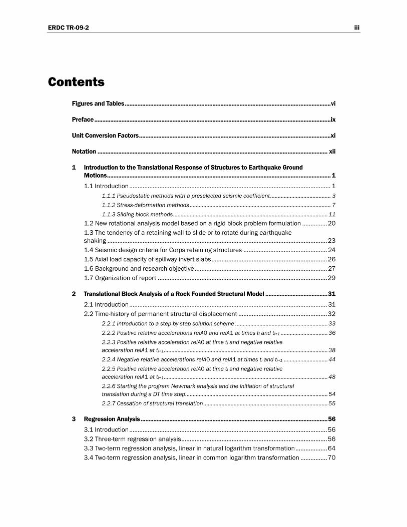
Contents Figures and Tables.................................................................................................................................vi

Preface....................................................................................................................................................ix

Unit Conversion Factors........................................................................................................................xi

Notation ................................................................................................................................................ xii

1 Introduction to the Translational Response of Structures to Earthquake Ground Motions............................................................................................................................................ 1 1.1 Introduction........................................................................................................................ 1

1.1.1 Pseudostatic methods with a preselected seismic coefficient........................................ 3 1.1.2 Stress-deformation methods ............................................................................................. 7 1.1.3 Sliding block methods......................................................................................................11

1.2 New rotational analysis model based on a rigid block problem formulation ...............20 1.3 The tendency of a retaining wall to slide or to rotate during earthquake shaking ...................................................................................................................................23 1.4 Seismic design criteria for Corps retaining structures .................................................. 24 1.5 Axial load capacity of spillway invert slabs.....................................................................26 1.6 Background and research objective............................................................................... 27 1.7 Organization of report .....................................................................................................29

2 Translational Block Analysis of a Rock Founded Structural Model .......................................31 2.1 Introduction...................................................................................................................... 31 2.2 Time-history of permanent structural displacement .....................................................32

2.2.1 Introduction to a step-by-step solution scheme .............................................................33 2.2.2 Positive relative accelerations relA0 and relA1 at times ti and ti+1 ...............................36 2.2.3 Positive relative acceleration relA0 at time ti and negative relative acceleration relA1 at ti+1............................................................................................................38 2.2.4 Negative relative accelerations relA0 and relA1 at times ti and ti+1 .............................44 2.2.5 Positive relative acceleration relA0 at time ti and negative relative acceleration relA1 at ti+1............................................................................................................48 2.2.6 Starting the program Newmark analysis and the initiation of structural translation during a DT time step..............................................................................................54 2.2.7 Cessation of structural translation..................................................................................55

3 Regression Analysis.....................................................................................................................56 3.1 Introduction......................................................................................................................56 3.2 Three-term regression analysis.......................................................................................56 3.3 Two-term regression analysis, linear in natural logarithm transformation...................64 3.4 Two-term regression analysis, linear in common logarithm transformation ................70

ERDC TR-09-2 iv

4 Regression results for ground motions recorded on rock.......................................................77 4.1 Introduction......................................................................................................................77 4.2 Regression results of earthquakes covering the Moment Magnitude (Mw) range of 6.9 – 8.1 (Magnitude 7)..........................................................................................89

4.2.1 Three-term regression results .........................................................................................90 4.2.2 Two-term regression results, linear in natural logarithm transformation .....................94 4.2.3 Two-term regression results, linear in common logarithm transformation ..................98 4.2.4 Comparison of regression results of all three forms of the simplified non-dimensionalized displacement relationships .........................................................................102

4.3 Regression results of earthquakes covering the Moment Magnitude (Mw) range of 6.1 – 6.8 (Magnitude 6)........................................................................................104

4.3.1 Three-term regression results .......................................................................................104 4.3.2 Two-term regression results, linear in natural logarithm transformation ...................108 4.3.3 Two-term regression results, linear in common logarithm transformation ................112 4.3.4 Comparison of regression results of all three forms of the simplified non-dimensionalized displacement relationships .........................................................................116

4.4 Regression results of earthquakes covering the Moment Magnitude (Mw) range from 4.9 – 6.1 (Magnitude 5) ...................................................................................118

4.4.1 Three-term regression results .......................................................................................118 4.4.2 Two-term regression results, linear in natural logarithm transformation ...................122 4.4.3 Two-term regression results, linear in common logarithm transformation ................126 4.4.4 Comparison of regression results of all three forms of the simplified non-dimensionalized displacement relationships. ........................................................................130

4.5 Special regression results of Equation Form Two of non-dimensionalized displacement relationships without differentiation of Moment Magnitude .....................131

4.5.1. Mean relationships .......................................................................................................132 4.5.2 Ninety-five percent probability of non-exceedance ......................................................134 4.5.3 Sixty-eight percent prediction intervals.........................................................................135

5 The Visual Modeler for Newmark – NewmarkVM.................................................................... 137 5.1 Introduction....................................................................................................................137 5.2 The Visual Modeling Environment ................................................................................137

5.2.1 Significant Tabs relevant to an analysis .......................................................................138 5.2.2 Multiple Horizontal Time-History Selections (Multiple Analyses only).........................139 5.2.3 Earthquake Time-History Horizontal Component 1 and 2 input (Single Analysis or Multiple Analyses) .................................................................................................143 5.2.4 Maximum Transmissible Acceleration input (Single Analysis or Multiple Analyses) ..................................................................................................................................146 5.2.5 The Selection of Time Histories (Multiple Analyses) ....................................................147 5.2.6 Analysis results (Single Analysis or Multiple Analyses)................................................149

5.3 Example 1 – Single Analysis or Sliding Block Analysis ................................................154 5.4 Example 2 – Multiple Analyses with Regression using Equation Form Two...............156

6 Conclusions and Recommendations ...................................................................................... 160 6.1 Introduction....................................................................................................................160 6.2 Ninety-five percent probability of non-exceedance......................................................160

6.2.1 Non-dimensionalized displacements of 23 sets of Moment Magnitude 7 group. ....................................................................................................................................160

ERDC TR-09-2 v

6.2.2 Non-dimensionalized displacements of 38 sets of Moment Magnitude 6 group .....................................................................................................................................161 6.2.3 Non-dimensionalized displacements of 66 sets of Moment Magnitude 5 group .....................................................................................................................................162 6.2.4 Non-dimensionalized displacements of 122 sets of Moment Magnitude 5 - 7 groups ..............................................................................................................................162

6.3 Mean relationships........................................................................................................164 6.3.1 Non-dimensionalized displacements of 23 sets of Moment Magnitude group 7 .....................................................................................................................................164 6.3.2 Non-dimensionalized displacements of 38 sets of Moment Magnitude group 6 .....................................................................................................................................165 6.3.3 Non-dimensionalized displacements of 66 sets of Moment Magnitude group 5 .....................................................................................................................................166 6.3.4 Non-dimensionalized displacements of 122 sets of Moment Magnitude 5 – 7 groups....................................................................................................................................166

6.4 Recommendations ........................................................................................................168

References......................................................................................................................................... 169

Appendix A: Listing and Description of the Newmark ASCII Input Data File (file name: Newmark.in)................................................................................................................................173

Appendix B: Listing of Newmark ASCII Data Output Files........................................................... 185

Report Documentation Page

ERDC TR-09-2 vi

Figures and Tables

Figures

Figure 1.1. Gravity retaining wall and “driving” soil wedge treated as a rigid body. ............................ 4 Figure 1.2. Simplified “driving” wedge method of analysis and the Mononobe-Okabe active earth pressure force relationship. ................................................................................................. 6 Figure 1.3. Elements of the Newmark (rigid) sliding block method of analysis .................................13 Figure 1.4. Gravity retaining wall and failure wedge treated as a sliding block ................................. 16 Figure 1.5. Incremental failure by base sliding .....................................................................................18 Figure 1.6. Idealized permanent, seismically induced displacement due to the rotation about the toe of a rock-founded wall retaining moist backfill, with toe restraint, computed using CorpsWallRotate.................................................................................................................................19 Figure 1.7. Rock-founded cantilever retaining wall bordering a spillway channel..............................20 Figure 1.8. Permanent, seismically induced displacement due to the rotation about the toe of a rock-founded, partially submerged cantilever retaining wall and with toe restraint, computed using CorpsWallRotate. .............................................................................................................22 Figure 1.9. Structural wedge with toe resistance retaining a driving soil wedge with a bilinear moist slope analyzed by effective stress analysis with full mobilization of shear resistance within the backfill...................................................................................................................23 Figure 2.1. Complete equations for relative motions over time increment DT based on linearly varying acceleration....................................................................................................................34 Figure 2.2. Relative Velocity and displacements at the end of time increment DT based on linearly varying relative acceleration. ..................................................................................................... 37 Figure 2.3. Two possible outcomes for the case of a negative relative acceleration at time ti and a positive relative acceleration at time ti+1. .................................................................................39 Figure 2.4. Two possible outcomes for the case of negative relative accelerations at times ti and ti+1. ...................................................................................................................................................45 Figure 2.5. Two possible outcomes for the case of a positive relative acceleration at time ti and a negative relative acceleration at time ti+1. ..................................................................................49 Figure 4.1. Non-dimensionalized displacements with the mean, 68 percent prediction intervals and 95 percent probability of non-exceedance curves.........................................................92 Figure 4.2. Non-dimensionalized displacements with the mean, 68 percent prediction intervals and 95 percent probability of non-exceedance curves.........................................................95 Figure 4.3. Non-dimensionalized displacements with the mean, 68 percent prediction intervals and 95 percent probability of non-exceedance curves.........................................................99 Figure 4.4. Non-dimensionalized displacements and comparisons of the means of the three regression analysis equations for Magnitude 7 earthquakes. ................................................103 Figure 4.5. Non-dimensionalized displacements with the mean, 68 percent prediction intervals and 95 percent probability of non-exceedance curves.......................................................105 Figure 4.6. Non-dimensionalized displacements with the mean, 68 percent prediction intervals and 95 percent probability of non-exceedance curves.......................................................110

ERDC TR-09-2 vii

Figure 4.7. Non-dimensionalized displacements with the mean, 68 percent prediction intervals and 95 percent probability of non-exceedance curves.......................................................114 Figure 4.8. Non-dimensionalized displacements and comparisons of the means of the three regression analysis equations for Magnitude 6 earthquakes. ................................................117 Figure 4.9. Non-dimensionalized displacements with the mean, 68 percent prediction intervals and 95 percent probability of non-exceedance curves.......................................................119 Figure 4.10. Non-dimensionalized displacements with the mean, 68 percent prediction intervals and 95 percent probability of non-exceedance curves.......................................................124 Figure 4.11. Non-dimensionalized displacements with the mean, 68 percent prediction intervals and 95 percent probability of non-exceedance curves.......................................................128 Figure 4.12. Non-dimensionalized displacements and comparisons of the means of the three regression analysis equations for Magnitude 5 earthquakes. ................................................131 Figure 4.13. Non-dimensionalized displacements for normalized earthquakes without differentiation of Moment Magnitude (Equation Form Two). .............................................................133 Figure 5.1. The Introduction tab features the process of a multiple analysis.................................138 Figure 5.2. The Multiple Horizontal Time-History Selections tab ready for user input. ...............140 Figure 5.3. Selection of horizontal time-history files...........................................................................142 Figure 5.4. Horizontal earthquake time-history ground motion shown in the Earthquake Time-History Horz Comp. 1 tab............................................................................................................144 Figure 5.5. Maximum Transmissible Acceleration tab for multiple analyses data entry. ............147 Figure 5.6. The Selection of Time Histories tab for data entry used for multiple analyses. .........148 Figure 5.7. The Analysis tab used for all analyses..............................................................................150 Figure 5.8. Single and combinations of three equations available for Regression Analyses. ........151 Figure 5.9. Illustrative example of Newmark during execution..........................................................152 Figure 5.10. Resultant output data from multiple analyses. .............................................................153 Figure 5.11. Resultant output data from a regression analysis. .......................................................153 Figure 5.12. The Analysis tab for Example 1. .....................................................................................154 Figure 5.13. Sliding block time-history results for Example 1............................................................155 Figure 5.14. The Analysis tab for Example 2. .....................................................................................157 Figure 5.15. Non-dimensionalized earthquake displacements. .......................................................158 Figure 5.16. The mean, 68 percent prediction intervals and 95 percent probability of non-exceedance.............................................................................................................................................159 Figure 6.1. 95 percent probability of non-exceedance relationships of non-dimensionalized displacements of four magnitude groups...............................................................163 Figure 6.2. Mean relationships of non-dimensionalized displacements of all four magnitude groups. .................................................................................................................................167

Tables

Table 1.1. Approximate magnitudes of movements required to reach minimum active earth pressure conditions (after Clough and Duncan 1991)................................................................. 5 Table 3.1. Forms of simplified non-dimensionalized permanent displacement relationships. ............................................................................................................................................56 Table 4.1. Master accelerograph table of magnitude 6.9 – 8.1..........................................................79

ERDC TR-09-2 viii

Table 4.2. Master accelerograph table of magnitude 6.1 – 6.8 earthquakes................................... 81 Table 4.3. Master accelerograph table of magnitude 4.9 – 6.1 earthquakes...................................84 Table 4.4. Sets of earthquake time-history data classified by moment magnitude ranges. ............89 Table 4.5. Comparison between the Richter and Moment Magnitude Scales. .................................89 Table 4.6. Values for the regression equations constants for Moment Magnitude (Mw) range of 6.9 – 8.1 (Magnitude 7). ..........................................................................................................90 Table 4.7. Values for the regression equations constants for Moment Magnitude (Mw) range of 6.1 – 6.8 (Magnitude 6). ........................................................................................................104 Table 4.8. Values for the regression equations constants for Moment Magnitude (Mw) range of 4.9 – 6.1 (Magnitude 5). ........................................................................................................118 Table 6.1. 95 percent probability percent of non-exceedance relationships of non-dimensionalized displacements of four magnitude groups...............................................................164 Table 6.2. Mean relationships of non-dimensionalized displacements of all four magnitude groups. .................................................................................................................................168 Table B.1. Output data files used by output buttons in the visual modeler analysis tab. ...............185

ERDC TR-09-2 ix

Preface

This research report describes the engineering formulation and corre-sponding software developed for the translational response of U.S. Army Corps of Engineers hydraulic structures to earthquake ground motions. The PC software Newmark was developed to perform an analysis of the permanent sliding displacement response for each structural feature (e.g., a rock-founded retaining wall section or a gravity dam section) to a user-specified earthquake acceleration time-history via a complete time-history analysis. PC software Newmark is also used in this R&D effort to perform a statistical analysis of computed permanent displacements for a suite of acceleration time-histories resulting in simplified (seismic) permanent displacement relationships for use in simplified sliding block analysis. This R&D was accomplished and the results summarized in this report for use on rock-founded structural systems. Prior to this publication, the simpli-fied permanent displacement relationships found in the technical litera-ture are for soil-founded structures. Funding to initiate research and soft-ware development and engineering study was provided by Headquarters, U.S. Army Corps of Engineers (HQUSACE), as part of the Flood and Coastal Storm Damage Reduction Research and Development Program. The research was performed under the Dam Safety Focus Area, Work Unit 142084 entitled “Simplified Probabilistic Models for Concrete Gravity Dams” for which Dr. Robert M. Ebeling, Computational Science and Engi-neering (CSED), Information Technology Laboratory (ITL), U.S. Army Engineer Research and Development Center (ERDC), was the Principal Investigator. Additional funding was provided by the Engineering Risk and Reliability Directory of Expertise. Andy Harkness (of Pittsburgh District), Technical Manager of the Engineering Risk and Reliability Directory of Expertise, supervised this R&D effort.

H. Wayne Jones, ITL, was the Dam Safety Focus Area Manager. William R. Curtis, Coastal and Hydraulics Laboratory (CHL), ERDC, was the Flood and Coastal Storm Damage Reduction Research and Develop-ment Program Manager, and Dr. Michael Sharp, Geotechnical and Structures Laboratory (GSL), ERDC, was the Water Resources Infra-structure Technical Director.

ERDC TR-09-2 x

The resulting engineering methodology and corresponding software is applicable to a variety of structural systems founded on rock. The main focus of this R&D effort was to develop simplified seismic permanent displacement relationships for rock-founded structures for use in a simpli-fied sliding block analysis. Although developed for the evaluation of the permanent displacement of rock-founded structures, PC software Newmark may also be used to compute the permanent displacement of soil-founded structures during earthquake shaking.

This R&D study was conducted by Dr. Robert M. Ebeling and Moira T. Fong, ITL, Donald E. Yule, GSL, Amos Chase, Sr., Science Applications International Corporation, and Raju Kala, GSL. Dr. Ebeling was author of the scope of work for this research. The report was prepared by Dr. Ebeling, Ms. Fong, and Mr. Yule under the supervision of Dr. Robert M. Wallace, Chief, CSED, and Dr. Reed Mosher, Director, ITL.

COL Gary E. Johnston was Commander and Executive Director of ERDC. Dr. James R. Houston was Director.

ERDC TR-09-2 xi

Unit Conversion Factors

Multiply By To Obtain

feet 0.3048 meters

inches 0.0254 meters

pounds (mass) 0.45359237 kilograms

ERDC TR-09-2 xii

Notation

A a decimal fraction

A • g the acceleration of the ground

angle β the direction of the resultant force S of the distributed shear stresses along the interface, as shown in Figure 1.3b

angle θ the angle inclination of the resultant inertia force ( = 0

for horizontal accelerations only)

Areaa the positive area under the linear relative acceleration relationship over the time step DT

Areav the positive area under the positive quadratic relative velocity relationship over the time step DT

β1, β2, β3, β4, β5 coefficients

c′ Mohr-Coulomb effective cohesion

COSMOS Consortium of strong-ground motion observation systems

Δt a time increment

DSHA a Deterministic Seismic Hazard Assessment

D, D1, D2, D3 the determinants of a matrix

dm permanent displacement (length)

ds the standardized maximum displacement

DT, dt time increments

DTzeroD a time increment

DTmid a time increment

ERDC TR-09-2 xiii

DTzeroV a time increment

FLAC a commercially available, two-dimensional, explicit finite difference program, which has been written primarily for geotechnical applications and applied to dynamic analysis of earthen systems

FLUSH a classic example of a category of software which uses the finite element method and treats the structure and the surrounding retained soil and foundation medium in a single analysis step; used in dynamic soil-structure in interaction analyses

G, g the acceleration of gravity

GUI Graphical User Interface

KAE pseudo-static active earth pressure coefficient

kc maximum transmissible acceleration capacity (decimal fraction)

kips 1,000 lbs

kh and kv decimal fraction that, when multiplied times the weight of some body, gives horizontal and vertical pseudo-static inertia force S for use in permanent seismic deformation analyses

kmg maximum horizontal ground acceleration

ks the standardized acceleration expressed as a fraction of g (o.5)

lhsDT Left-hand side time increment

ln the natural log

MCE Maxim Credible Earthquake

MDE Maximum Design Earthquake

Ms surface wave

ERDC TR-09-2 xiv

Mw moment magnitude scale

N a decimal fraction of the acceleration imparted to the Figure 1.3a soil sliding mass

N the total number of non-dimensionalized displacement terms in Figure 3.7

N*g the maximum transmissible horizontal acceleration (a constant)

OBE Operational Basis Earthquake

P the force that is a resultant of the normal forces shown in Figure 1.3b

PEER Pacific Earthquake Engineering Research Center

P • Δ second-order structural deformation effects

φ Mohr-Coulomb angle of internal friction shear strength parameter

φ′ Mohr-Coulomb effective angle of internal friction shear

strength parameter

PSHA Probabilistic Seismic Hazard Analysis

Presist a user-defined force representing the ultimate axial load resistance of a slab

relA relative acceleration

relA0, relA1 relative acceleration values at times ti and ti+1,

respectively

relAmid midrange relative acceleration

relD relative displacement

relD0 from the value for relative displacement at time ti

relD1 the permanent relative structural displacement at time

ti+1

ERDC TR-09-2 xv

relDmid midrange relative displacement

relV relative velocity

relV0 relative velocity at time ti

relV1 relative velocity at time ti+1

relVmid midrange relative velocity

rhsDT right-hand side time increment

S the resultant force of the distributed shear stresses along the interface, Figure 1.3c

SHAKE a vertical shear wave propagation program

SOILSTRUCT an Incremental Construction, Soil-Structure Interaction finite element program

SSI a soil-structure interaction

Su undrained shear strength of soils

ti, ti+1, Δt timesteps

vm the maximum ground velocity

vr the relative velocity of a wall

vs the standardized velocity (29.92 in./sec)

Vs average shear wave velocity

W the weight of the sliding mass, as shown in Figure 1.3a

ERDC TR-09-2 1

1 Introduction to the Translational Response of Structures to Earthquake Ground Motions

1.1 Introduction

Engineering formulations and software provisions based on sound seismic engineering principles are needed for a wide variety of rock-founded Corps hydraulic structures that translate (i.e., slide) or rotate during earthquake shaking and for massive concrete structures constrained to rocking. The engineering formulation discussed in this report was developed to address the first of these three different modes of structural responses to earth-quake shaking.

This research report describes the development of simplified permanent deformation relationships for rock-founded structures subjected to earth-quake shaking. The original permanent (translational) deformation pro-cedure of analysis, published by Newmark in 1965, required the use of an earthquake acceleration time-history in order to predict the permanent deformation of a structure (an earthen slope of an embankment in Professor Newmark’s examples). This type of analysis is referred to as a “Complete Time-History Permanent (Translational) Displacement Analysis” and is a capability of the PC software developed in support of the R&D discussed in this report. The drawback to a complete time-history permanent deformation analysis is that there are many factors to consider and many stages to the selection of earthquake acceleration time histories for use on a Corps project. Additionally, the time-history selection process requires information that typically is not readily available at the beginning of a Corps project effort. Fortunately, there is an alternative procedure of seismically induced permanent deformation analysis available to District engineers for use on Corps projects. This alternative procedure requires only rudimentary design/analysis ground motion characterization and use of a simplified permanent seismic displacement relationship for a sliding block (structural) system model. This simplified seismic permanent (translational) deformation procedure of analysis was developed for the Corps in 1977 by the WES/ERDC researchers Dr. Franklin and Mr. Chang.

ERDC TR-09-2 2

In a subsequent study to that conducted by Newmark (1965), Franklin and Chang (1977) expanded the use of the permanent seismically induced deformation procedure of analysis through the development of “Simplified Sliding Block” relationships. In order to use the Franklin and Chang rela-tionships (which are for computed data presented in figure form), values for peak ground acceleration and peak ground velocity are required. A “Simplified Sliding Block” formulation has the advantage of eliminating the need for the Engineer to directly select an acceleration time-history to characterize earthquake shaking. The Franklin and Chang permanent deformation relationships are a direct product of an evaluation process involving acceleration time histories. Results of their calculations reflect the use of many acceleration time histories. Note that only acceleration time histories recorded during earthquakes occurring through 1977 were included in their study.

Two drawbacks to using the Franklin and Chang (1977) “Simplified Sliding Block” relationships for rock-founded structural systems exist; the focus of the relationships they developed is on soil sites (reflecting the early days when the permanent sliding block displacement based method of analysis was first applied to earthen “structural” systems consisting of slopes and earthen embankments); and since 1977 there have been a number of earthquake events recorded on rock as well as soil sites.

In the subsequent years there have been several studies resulting in seis-mically induced simplified permanent sliding block relationships, but all of these studies have been dominated by the use of soil site acceleration time-history records (e.g., Makdisi and Seed 1978; Richards and Elms 1979; Whitman and Liao 1985a, 1985b; Ambraseys and Menu 1988; Cai and Bathurst 1996). This research report summarizes the development of seismically induced, simplified sliding block permanent deformation rela-tionships for rock-founded structures and is accomplished by processing data obtained by using a collection of acceleration time histories recorded on different “rock” sites. One hundred and twenty-two sets of horizontal “rock” acceleration time histories recorded during many different earth-quake events were carefully selected, base-line corrected and processed (as discussed in Chapter 4) using the PC software Newmark to develop the simplified permanent sliding block displacement relationships summa-rized in Chapter 6 of this report.

ERDC TR-09-2 3

The resulting simplified permanent deformation relationships for rock-founded structures summarized in this report will be implemented within CorpsWallSlip (Ebeling et al. 2007) and within CorpsDamSlip (in development by Ebeling and Chase) for the seismic Simplified Sliding Block analysis of rock-founded earth retaining structures and rock-founded concrete gravity dams, respectively.

There are three categories of analytical approaches used to perform a seismic stability analysis. They are listed in order of sophistication and complexity:

• Pseudostatic methods with a preselected seismic coefficient. • Stress-deformation methods. • Sliding block methods.

Each category will be subsequently discussed so as to put the Newmark sliding block method of analysis in perspective as well as understand some of the input data requirements for the PC software Newmark developed for use in this R&D effort and described in this report. Because sliding block methods are the focus of this report, it will be discussed last. The examples to be discussed will involve either embankment slopes or earth retaining structures.

1.1.1 Pseudostatic methods with a preselected seismic coefficient

Pseudostatic methods with a preselected seismic coefficient in the hori-zontal and in the vertical direction often require bold assumptions about the manor in which the earthquake shaking is represented and the simpli-fications made for their use in stability computations. Essentially, it is a force equilibrium method of analysis expressing the safety and stability of an earth retaining structure to dynamic earth forces in terms of the following:

• The factor of safety against sliding along the base of the wall, • The ability of the wall to resist the earth forces acting to overturn the

wall, • The factor of safety against a bearing capacity failure or crushing of the

concrete or rock at the toe in the case of a rock foundation.

An example using 1992 Corps criteria (now outdated) is discussed in Section 6.2 of Chapter 6 in Ebeling and Morrison (1992). Pseudostatic

ERDC TR-09-2 4

methods with horizontal and vertical preselected seismic coefficients represent earthquake loading as static forces.

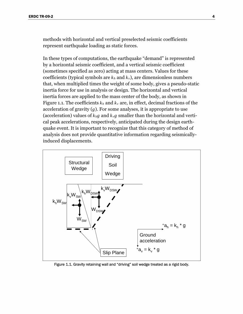
In these types of computations, the earthquake “demand” is represented by a horizontal seismic coefficient, and a vertical seismic coefficient (sometimes specified as zero) acting at mass centers. Values for these coefficients (typical symbols are kh and kv), are dimensionless numbers that, when multiplied times the weight of some body, gives a pseudo-static inertia force for use in analysis or design. The horizontal and vertical inertia forces are applied to the mass center of the body, as shown in Figure 1.1. The coefficients kh and kv are, in effect, decimal fractions of the acceleration of gravity (g). For some analyses, it is appropriate to use (acceleration) values of khg and kvg smaller than the horizontal and verti-cal peak accelerations, respectively, anticipated during the design earth-quake event. It is important to recognize that this category of method of analysis does not provide quantitative information regarding seismically-induced displacements.

Driving

Soil

Wedge

StructuralWedge

WSW

WDSW

khWSW

kvWSWkhWDSW

kvWDSW

Slip Plane

Groundacceleration

+ah = kh * g

+av = kv * g

Figure 1.1. Gravity retaining wall and “driving” soil wedge treated as a rigid body.

ERDC TR-09-2 5

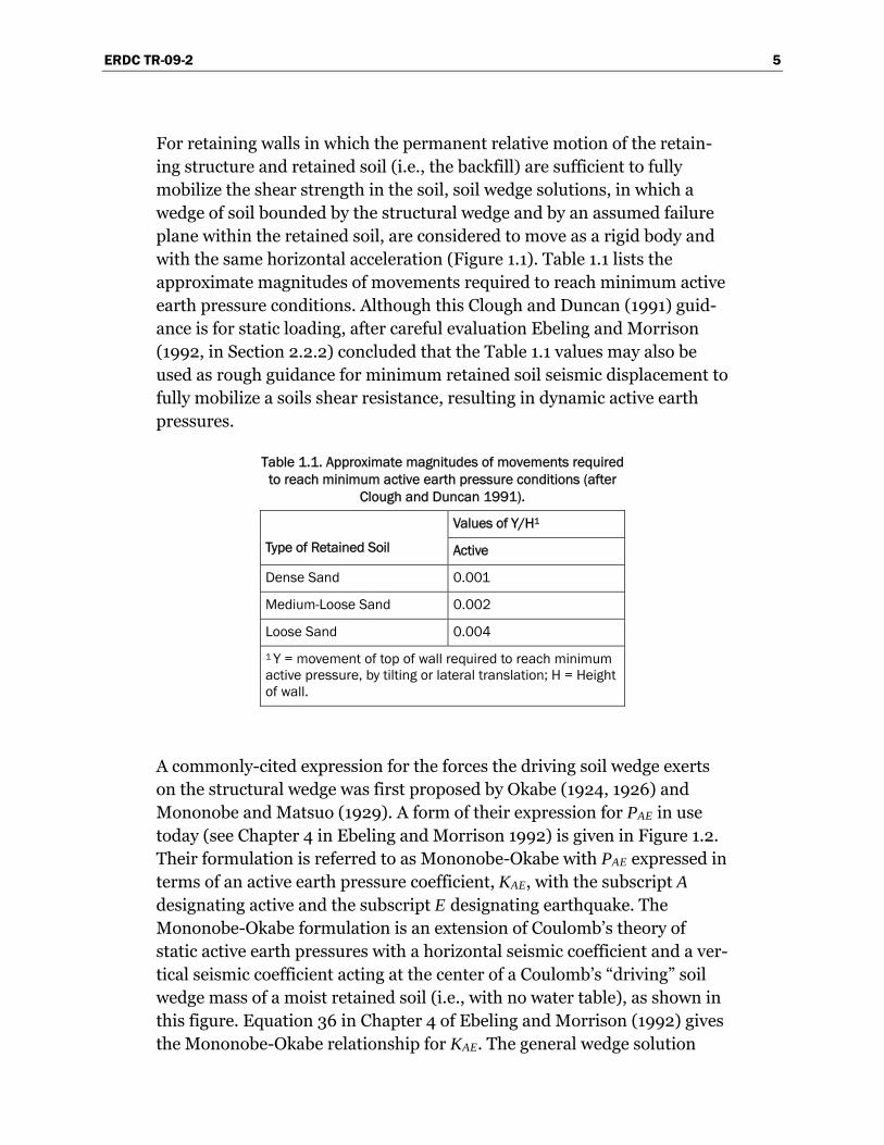
For retaining walls in which the permanent relative motion of the retain-ing structure and retained soil (i.e., the backfill) are sufficient to fully mobilize the shear strength in the soil, soil wedge solutions, in which a wedge of soil bounded by the structural wedge and by an assumed failure plane within the retained soil, are considered to move as a rigid body and with the same horizontal acceleration (Figure 1.1). Table 1.1 lists the approximate magnitudes of movements required to reach minimum active earth pressure conditions. Although this Clough and Duncan (1991) guid-ance is for static loading, after careful evaluation Ebeling and Morrison (1992, in Section 2.2.2) concluded that the Table 1.1 values may also be used as rough guidance for minimum retained soil seismic displacement to fully mobilize a soils shear resistance, resulting in dynamic active earth pressures.

Table 1.1. Approximate magnitudes of movements required to reach minimum active earth pressure conditions (after

Clough and Duncan 1991).

Values of Y/H1

Type of Retained Soil Active

Dense Sand 0.001

Medium-Loose Sand 0.002

Loose Sand 0.004

1 Y = movement of top of wall required to reach minimum active pressure, by tilting or lateral translation; H = Height of wall.

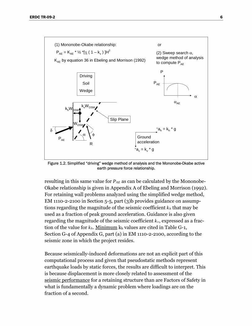
A commonly-cited expression for the forces the driving soil wedge exerts on the structural wedge was first proposed by Okabe (1924, 1926) and Mononobe and Matsuo (1929). A form of their expression for PAE in use today (see Chapter 4 in Ebeling and Morrison 1992) is given in Figure 1.2. Their formulation is referred to as Mononobe-Okabe with PAE expressed in terms of an active earth pressure coefficient, KAE, with the subscript A designating active and the subscript E designating earthquake. The Mononobe-Okabe formulation is an extension of Coulomb’s theory of static active earth pressures with a horizontal seismic coefficient and a ver-tical seismic coefficient acting at the center of a Coulomb’s “driving” soil wedge mass of a moist retained soil (i.e., with no water table), as shown in this figure. Equation 36 in Chapter 4 of Ebeling and Morrison (1992) gives the Mononobe-Okabe relationship for KAE. The general wedge solution

ERDC TR-09-2 6

α

P

PAE

αAE

Driving

Soil

Wedge

WDSW

khWDSWkvWDSW

Slip Plane

PAE

δα

R

φ Groundacceleration

+ah = kh * g

+av = kv * g

(1) Mononobe-Okabe relationship:

PAE = KAE * ½ *[γt ( 1 – kv ) ]H2

KAE by equation 36 in Ebeling and Morrison (1992)

or

(2) Sweep search α,wedge method of analysisto compute PAE

Figure 1.2. Simplified “driving” wedge method of analysis and the Mononobe-Okabe active

earth pressure force relationship.

resulting in this same value for PAE as can be calculated by the Mononobe-Okabe relationship is given in Appendix A of Ebeling and Morrison (1992). For retaining wall problems analyzed using the simplified wedge method, EM 1110-2-2100 in Section 5-5, part (3)b provides guidance on assump-tions regarding the magnitude of the seismic coefficient kh that may be used as a fraction of peak ground acceleration. Guidance is also given regarding the magnitude of the seismic coefficient kv, expressed as a frac-tion of the value for kh. Minimum kh values are cited in Table G-1, Section G-4 of Appendix G, part (a) in EM 1110-2-2100, according to the seismic zone in which the project resides.

Because seismically-induced deformations are not an explicit part of this computational process and given that pseudostatic methods represent earthquake loads by static forces, the results are difficult to interpret. This is because displacement is more closely related to assessment of the seismic performance for a retaining structure than are Factors of Safety in what is fundamentally a dynamic problem where loadings are on the fraction of a second.

ERDC TR-09-2 7

1.1.2 Stress-deformation methods

Stress-deformation methods are specialized applications of finite element or finite difference programs for the dynamic analysis of earth retaining structures to seismic loading using numerical techniques to account for the nonlinear engineering properties of soils. The problem being analyzed is often referred to as a soil-structure interaction (SSI) problem. Accelera-tion time histories are typically used to represent the earthquake ground motions in this type of formulation. The general procedure of stress-deformation dynamic analysis is straightforward and follows the usual engineering approach:

1. Define the problem, 2. Idealize the physical system, 3. Set up the equations of motion for the dynamic problem, 4. Characterize the dynamic engineering properties of the (structure, soil,

and/or rock) materials as per the constitutive material model(s) being used,

5. Solve the equations of motion, 6. Evaluate the results.

Steps (1), (2), (4) and (6) are handled by the engineer while steps (3) and (5) are dealt with by the engineering software. A partial listing of computer-based codes for dynamic analysis of soil systems are given in Appendix D of Ebeling and Morrison (1992). Use of this type of advanced engineering software requires specialized knowledge in the fields of geotechnical and structural engineering dynamics as well as in numerical methods. Two computer programs, FLUSH and FLAC, will be discussed briefly to give the reader a sense of what is involved with the application of computationally complex numerical codes in a complete soil-structure interaction dynamic analysis and the numerous input and modeling considerations required.

1.1.2.1 FLUSH

The American Society of Civil Engineers (ASCE) Standard 4-86 (1986) states that SSI denotes the phenomenon of coupling between a structure and its supporting soil or rock medium during earthquake shaking. The resulting dynamic soil pressures are a result of the degree of interactions that occur between the structure and the soil. This response is dependent on the following:

ERDC TR-09-2 8

• The characteristics of the ground motion • The retained and foundation soils (or rock) • The structure itself.

One method of analysis for SSI is referred to as the Direct method and treats the structure and the surrounding retained soil and foundation medium in a single analysis step. FLUSH is a classic example of this cate-gory of software which uses the finite element method in this dynamic analysis (Lysmer et al. 1975).

Two-dimensional (2-D) cross-sections of the retaining structure, and por-tions of the retained soil and foundation, are typically modeled in the FLUSH analysis. Nonlinear soil behavior is treated through equivalent linearization of the shear stiffness of each soil element, with the effective shear strains that develop during earthquake shaking, for the user speci-fied earthquake acceleration time-history. Material damping is assigned to each soil (and/or rock) element and to each structural element comprising the mesh. Material damping is strain-compatible for each soil, rock and structural material type. FLUSH solves the equation of motion in the fre-quency domain. The acceleration time-history is introduced through the base nodes of the mesh; fictitious (artificial) boundary conditions that allow for the introduction of vertically propagating shear waves resulting in horizontal motion of the nodes of the mesh during earthquake shaking, and for vertically propagating compression waves that allow for the verti-cal motion of the nodes. Lateral boundaries are referred to as transmitting boundaries and are imposed on the 2-D mesh to allow for energy absorb-ing boundary conditions to be specified. Because it is essentially a wave propagation problem being solved, great care is exercised by the seismic engineer to size the mesh so that moderate to high wave frequencies are not artificially excluded in the dynamic numerical analysis. Sizing of the 2-D mesh, as it pertains to the height of the elements and with regard to the maximum shear wave frequency vertically transmitted by the ele-ments, first involves the analysis of representative one-dimensional (1-D) soil columns.

To assess the maximum frequency that may be transmitted by a user-proposed 2-D finite element mesh in a FLUSH analysis, representative imaginary section(s) within the 2-D model problem are first analyzed by the vertical shear wave propagation program SHAKE (Schnabel et al. 1972) and by a 1-D finite element column using FLUSH. Strain-compatible

ERDC TR-09-2 9

shear stiffness results from the SHAKE analyses are used to determine the maximum height of the soil elements for the maximum frequency of the vertically propagating shear wave needed to be transmitted in the FLUSH (2-D) analysis. A 1-D soil column is then constructed using finite elements and analyzed using FLUSH to verify that the required vertically propagat-ing shear wave frequencies are being transmitted by the FLUSH mesh. The wavelength associated with the highest frequency transmitted by the mesh is related to the heights of the elements and to the (strain compatible) shear wave velocities via the strain compatible shear stiffness of each of the elements. Recall that FLUSH accounts for nonlinear response of soils during earthquake shaking through adjustments of the soil shear stiffness and material damping parameters as a function of shear strain that develop in each element of the finite element mesh. Note that the results of this assessment are dependent on the characteristics of the acceleration time-history used in the analysis.

FLUSH output obtained via the extraction mode includes time-histories of the dynamic stresses within each element and dynamic displacements at each node in the finite element model. Time-histories of nodal point forces may also be obtained using specialized software. The computed dynamic stresses are then superimposed on the static stresses to attain the total stresses. Static stresses are typically obtained from a SOILSTRUCT finite element analysis (Ebeling et al. 1992).

In a static analysis using SOILSTRUCT, the nonlinear stress-strain behavior of soils are accounted for in an incremental, equivalent linear method of analysis in which the sequential excavation (if any), followed by sequential construction of the structure and incremental placement of retained soil, is made. Examples of this application to Corps structures for static loading(s) are given in Clough and Duncan (1969), Ebeling et al. (1993); Ebeling and Mosher (1996); Ebeling and Wahl (1997); Ebeling et al. (1997b); and Ebeling et al. (1997c). The mesh used in the FLUSH dynamic analysis will be the basis for the mesh used in the SOILSTRUCT static analysis, for the convenience of combining results.

1.1.2.2 FLAC

In 1992, the Corps completed its first research application of FLAC to the seismic analysis of a cantilever retaining wall (Green and Ebeling 2002). FLAC is a commercially available, two-dimensional, explicit finite differ-ence program, which has been written primarily for geotechnical

ERDC TR-09-2 10

applications. The basic formulation of FLAC is plane-strain. Dynamic analyses can be performed with FLAC using an optional dynamic calcula-tion module, wherein user-specified acceleration, velocity, or stress time-histories can be input as an exterior boundary condition or as an interior excitation. FLAC allows for energy absorbing boundary conditions to be specified, which limits the numerical reflection of seismic waves at the model perimeter. The nonlinear constitutive models (10 are built-in), in conjunction with the explicit solution scheme, in FLAC give stable solu-tions to unstable physical processes, such as sliding or overturning of a retaining wall. FLAC solves the full dynamic equations of motion, even for essentially static systems, which enables accurate modeling of unstable processes, e.g., retaining wall failures.

FLAC, like FLUSH, has restrictions associated with the wavelength asso-ciated with the highest frequency transmitted within the grid. A procedure similar to that used to design the FLUSH mesh and involving 1-D soil column analyses, via SHAKE, is used to lay out the FLAC grid for the dynamic retaining wall problem analyzed and for the specified accelera-tion time-history. Section 3.3.4 of Green and Ebeling (2002) discuss the dimensions of the finite difference grid and the maximum frequency that can pass through without numerical distortion.

A disadvantage of FLAC is the long computational times, particularly when modeling stiff materials, which have large physical wave speeds. The size of the time-step depends on the dimension of the elements, the wave speed of the material, and the type of damping specified (i.e., mass pro-portional or stiffness proportional), where stiffness proportional, to include Rayleigh damping, requires a much smaller time step. The critical time step for numerical stability and accuracy considerations is auto-matically computed by FLAC, based on these factors listed. For those readers unfamiliar with the concept of critical time-step for numerical stability and accuracy considerations in a seismic time-history engineering analysis procedure, please refer to Ebeling (1992), Part V, or to Ebeling et al. (1997a). The Lagrangian formulation in FLAC updates the grid coordinates each time-step, thus allowing large cumulative deformations to be modeled. This is in contrast to Eularian formulation in which the material moves and deforms relative to a fixed grid, and is therefore limited to small deformation analyses.

ERDC TR-09-2 11

1.1.2.3 FLUSH versus FLAC

The advantages of FLUSH are that it has considerably faster run times than FLAC and has been applied to a number of dynamic SSI problems. FLUSH is now freely downloadable from the Internet. The major dis-advantage of FLUSH is that it does not allow for permanent displacement of the wall (although strain softening associated with earthquake-induced soil or rock deformations are accounted for in the analysis). A disadvan-tage of FLAC is that the earthquake engineering community and the Corps is just now developing modeling procedures for the application of FLAC to dynamic SSI problems, learning how to perform the analyses and interpret the computed results.

1.1.3 Sliding block methods

Sliding block methods of analysis of earth retaining structures can be viewed as a compromise between the simplistic pseudostatic methods, with a preselected seismic coefficient, and the computationally complex finite element or finite-difference based stress-deformation methods of analysis. Sliding block methods of analysis calculate a permanent defor-mation of a retaining structural system initiated by a user specified design earthquake event.

The numerous variations of rigid sliding block methods of seismic analysis as applied to slopes, earthen dams, retaining wall systems, and founda-tions have their roots in the methodology outlined in Newmark (1965) and what has come to be known as the Newmark sliding block model.1 This problem was first studied in detail by Newmark (1965) using the sliding block on a sloping plane analogy. Procedural refinements were contributed by Franklin and Chang (1977); Wong (1982); Whitman and Liao (1985a, 1985b); Ambraseys and Menu (1988); and others. Makdisi and Seed (1978) and Idriss (1985, Figure 47) proposed relationships based on a modification to the Newmark permanent displacement procedure to allow for dynamic response considerations.

1 An interesting footnote in seismic engineering history is given in Whitman (2000): Dr. Robert Whitman,

Professor Emeritus of MIT, in 1953 performed a calculation of the permanent displacement of a slope as a result of earthquake-induced ground motions using a sliding block concept for a consulting job that Professor Donald Taylor (of MIT) had with the U.S. Army Corps of Engineers. Professor Newmark was part of the same consulting panel and sent word back to Dr. Whitman that he found this approach to be interesting, and that if he (Whitman) did not pursue it, he (Newmark) would. Dr. Whitman did not, and Professor Newmark did. Professor Newmark’s research culminated in his (now classic) 1965 Geotechnique paper on this topic, the fifth Rankine lecture.

ERDC TR-09-2 12

1.1.3.1 Concepts of Newmark’s sliding (rigid) block method of analysis

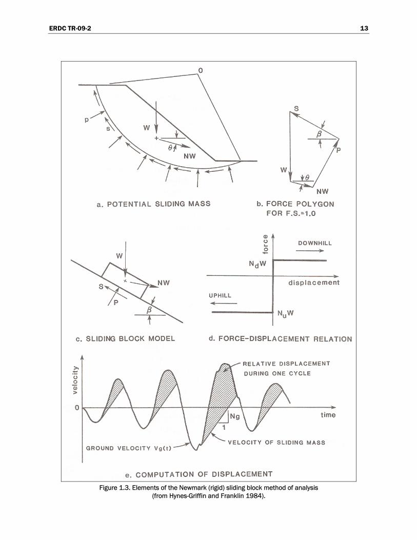
Franklin and Chang (1977) and Hynes-Griffin and Franklin (1984) illu-strate key concepts of a Newmark sliding block analysis using a potential sliding mass within an embankment under earthquake loading. The problems’ engineering idealization is shown in Figure 1.3. The Figure 1.3a potential sliding mass is in a condition of incipient sliding with full mobil-ization of the shear resistance for the soil along the slip plane shown in this figure. The corresponding sliding factor of safety is equal to unity. This condition results from the acceleration of the earthen mass into the embankment (i.e., to the left) and away from the cut. W is the weight of the sliding mass. The force N times W in this figure is the inertia force required to reduce the sliding factor of safety to unity. By D’Alembert’s principle, the inertia force, N times W, is applied pseudostatically to the soil mass in a direction opposite to acceleration of the mass, N times g, with N being a decimal fraction of the acceleration of gravity g (the uni-versal gravitational constant). The acceleration of the soil mass contained within the slip plane shown in Figure 1.3a is limited to an acceleration value of N times g because the shear stress required for equilibrium along the slip plane can never be less than that of the shear strength of the soil. To state this in another way, the sliding factor of safety can never be less than 1.0. So, if the earthquake induced ground acceleration should increase to a value greater than the value N times g, the Figure 1.3a mass above this slip plane would move downhill relative to the embankment. During this permanent slope displacement, the “sliding” mass would only feel the acceleration value N times g and not the ground acceleration values. The acceleration value of N times g was referred to as the “yield acceleration” in these early publications associated with the seismically induced permanent movement of a slope.

Figure 1.3b shows the force polygon for the “sliding” soil mass. The angle inclination θ of the inertia force may be found as the angle that is most critical; that is, the angle that minimizes N. Franklin and Chang (1977) and Hynes-Griffin and Franklin (1984) state that the angle θ is typically set equal to zero in seismic slope stability analyses. The angle β is the direction of the resultant force S of the distributed shear stresses along the interface and is determined during the course of the slope stability anal-yses to determine the value of N that results in a sliding factor of safety of 1.0 for the slope’s sliding mass. The force P is the resultant of the normal forces.

ERDC TR-09-2 13

Figure 1.3. Elements of the Newmark (rigid) sliding block method of analysis

(from Hynes-Griffin and Franklin 1984).

ERDC TR-09-2 14

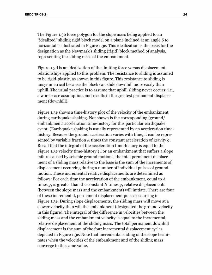
The Figure 1.3b force polygon for the slope mass being applied to an “idealized” sliding rigid block model on a plane inclined at an angle β to horizontal is illustrated in Figure 1.3c. This idealization is the basis for the designation as the Newmark’s sliding (rigid) block method of analysis, representing the sliding mass of the embankment.

Figure 1.3d is an idealization of the limiting force versus displacement relationships applied to this problem. The resistance to sliding is assumed to be rigid-plastic, as shown in this figure. This resistance to sliding is unsymmetrical because the block can slide downhill more easily than uphill. The usual practice is to assume that uphill sliding never occurs; i.e., a worst-case assumption, and results in the greatest permanent displace-ment (downhill).

Figure 1.3e shows a time-history plot of the velocity of the embankment during earthquake shaking. Not shown is the corresponding (ground/ embankment) acceleration time-history for this particular earthquake event. (Earthquake shaking is usually represented by an acceleration time-history. Because the ground acceleration varies with time, it can be repre-sented by variable fraction A times the constant acceleration of gravity g. Recall that the integral of the acceleration time-history is equal to the Figure 1.3e velocity time-history.) For an embankment that suffers a slope failure caused by seismic ground motions, the total permanent displace-ment of a sliding mass relative to the base is the sum of the increments of displacement occurring during a number of individual pulses of ground motion. These incremental relative displacements are determined as follows: For each time the acceleration of the embankment, equal to A times g, is greater than the constant N times g, relative displacements (between the slope mass and the embankment) will initiate. There are four of these incremental, permanent displacement pulses occurring in Figure 1.3e. During slope displacements, the sliding mass will move at a slower velocity than will the embankment (designated the ground velocity in this figure). The integral of the difference in velocities between the sliding mass and the embankment velocity is equal to the incremental, relative displacement of the sliding mass. The total permanent downhill displacement is the sum of the four incremental displacement cycles depicted in Figure 1.3e. Note that incremental sliding of the slope termi-nates when the velocities of the embankment and of the sliding mass converge to the same value.

ERDC TR-09-2 15

Summary: The idealized engineering problem depicted in Figure 1.3 describes the essential features of the Newmark sliding (rigid) block method of analysis as first applied to slopes:

• There is a level of earthquake shaking as characterized in terms of a value of acceleration designated N times g (i.e., the yield acceleration), which fully mobilizes the shear resistance along a sliding plane of a potential sliding mass; corresponding to a factor of safety against sliding of 1.0 for that mass.

• For a given embankment (or equivalently, ground) acceleration time-history in which acceleration(s) exceed the value of N times g, incre-mental permanent displacements will occur.

• The magnitude of the incremental displacements may be numerically quantified using the procedure outlined in Figure 1.3e.

• Total permanent displacement is equal to the sum of the incremental displacement pulses.

Although this procedure has been applied to other types of structures, the essential features of the Newmark (rigid) sliding block method of analysis remain the same.

1.1.3.2 Sliding block method of analysis applied to retaining structures

A variation proposed on the Newmark sliding block method of analysis for earth retaining structures is the displacement controlled approach (Section 6.3 in Ebeling and Morrison 1992). It incorporates retaining wall movements explicitly determined in the stability analysis of earth retain-ing structures. This methodology is applied as either the displacement-controlled design of (a new) retaining wall, or as an analysis of earthquake induced displacements of an existing retaining wall.

• The displacement controlled design of retaining wall: In this approach, the retaining wall geometry is the primary variable. It is, in effect, a procedure for choosing a seismic coefficient based upon explicit choice of an allowable permanent displacement. Having selected the seismic coefficient, the usual stability analysis against sliding is performed, including the use of the Mononobe-Okabe equations (or, alternatively, a sweep search, soil wedge solution). The wall is proportioned to resist the applied earth and inertial force loadings. No safety factor is required to be applied to the required weight of wall evaluated by this approach; the appropriate level of

ERDC TR-09-2 16

safety is incorporated into the step used to calculate the horizontal seismic coefficient. This procedure of analysis represents an improved alternative to the conventional equilibrium method of analysis that expresses the stability of a rigid wall (of prescribed geometry and mate-rial properties) in terms of a pseudostatic method with a preselected seismic coefficient and preselected factor of safety against sliding along its base, discussed in Section 1.1.1. Section 6.3.1 in Ebeling and Morrison (1992) outlines the computational steps in the (seismic) displacement controlled design of a retaining wall.

• The analysis of earthquake induced displacements of a retaining wall: The retaining wall geometry and material properties are typically first established for the usual, unusual and extreme load cases with non-seismic loadings. In the subsequent seismic analysis of the retaining wall using the earthquake induced displacement approach, the primary variable is the permanent displacement. The seismic inertia coefficient N* that reduces the sliding factor of safety for the driving soil wedge and the structural wedge to unity is first determined. Ebeling and Morrison (1992), along with others, have designated the acceleration value N*g for a retaining wall as its “maxi-mum transmissible acceleration.” Figure 1.4 shows the driving soil wedge and structural wedge treated as a single rigid block in this approach.

Groundacceleration

+ah = kh * g

+av = kv * g

Driving

Soil

Wedge

StructuralWedge

N*gN*g

Slip Plane

RetainedSoil

Movementof

Rigidblock

Note: Slip occurs when ah > N*g

Figure 1.4. Gravity retaining wall and failure wedge treated as a sliding block (after Whitman 1990).

ERDC TR-09-2 17

The resulting permanent seismic displacement of the retaining wall is sub-sequently determined for the earthquake specified by the design engineer. Section 6.3.2 in Ebeling and Morrison (1992) outlines the computational steps in the analysis of earthquake induced displacements of a retaining wall (with specified geometry and material properties).

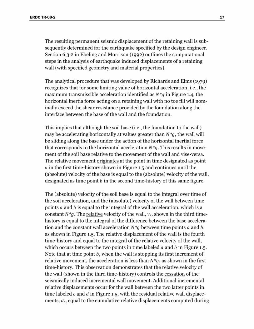
The analytical procedure that was developed by Richards and Elms (1979) recognizes that for some limiting value of horizontal acceleration, i.e., the maximum transmissible acceleration identified as N*g in Figure 1.4, the horizontal inertia force acting on a retaining wall with no toe fill will nom-inally exceed the shear resistance provided by the foundation along the interface between the base of the wall and the foundation.

This implies that although the soil base (i.e., the foundation to the wall) may be accelerating horizontally at values greater than N*g, the wall will be sliding along the base under the action of the horizontal inertial force that corresponds to the horizontal acceleration N*g. This results in move-ment of the soil base relative to the movement of the wall and vise-versa. The relative movement originates at the point in time designated as point a in the first time-history shown in Figure 1.5 and continues until the (absolute) velocity of the base is equal to the (absolute) velocity of the wall, designated as time point b in the second time-history of this same figure.

The (absolute) velocity of the soil base is equal to the integral over time of the soil acceleration, and the (absolute) velocity of the wall between time points a and b is equal to the integral of the wall acceleration, which is a constant N*g. The relative velocity of the wall, vr, shown in the third time-history is equal to the integral of the difference between the base accelera-tion and the constant wall acceleration N*g between time points a and b, as shown in Figure 1.5. The relative displacement of the wall is the fourth time-history and equal to the integral of the relative velocity of the wall, which occurs between the two points in time labeled a and b in Figure 1.5. Note that at time point b, when the wall is stopping its first increment of relative movement, the acceleration is less than N*g, as shown in the first time-history. This observation demonstrates that the relative velocity of the wall (shown in the third time-history) controls the cessation of the seismically induced incremental wall movement. Additional incremental relative displacements occur for the wall between the two latter points in time labeled c and d in Figure 1.5, with the residual relative wall displace-ments, dr, equal to the cumulative relative displacements computed during

ERDC TR-09-2 18

Figure 1.5. Incremental failure by base sliding (adapted from Richards and Elms 1979).

the entire time of earthquake shaking (labeled as point d in the fourth time-history). Lastly, although N*g is referred to as the maximum trans-missible acceleration in retaining structure permanent deformation problems, it is equivalent to the yield acceleration that is associated with permanent deformation problems for slopes/embankments. In the permanent deformation research conducted by Cai and Bathurst (1996), the term “critical acceleration” was used. The terms critical acceleration, maximum transmissible acceleration and yield acceleration all describe the same quantity.

Ebeling and Morrison (1992) observe that the approach has been reason-ably well validated for the case of walls retaining granular, moist backfills (i.e., no water table). A key item is the selection of suitable shear strength parameters. In an effective stress analysis, the issue of the suitable friction angle is particularly troublesome when the peak friction angle is signifi-cantly greater than the residual friction angle. In the displacement con-trolled approach examples given in Section 6.2 of Ebeling and Morrison (1992), effective stress based shear strength parameters (i.e., effective cohesion c′ and effective angle of internal friction φ′) were used to define the shear strength of the dilative granular backfills, with c′ set equal to zero in all cases due to the level of deformations anticipated in a sliding block analysis during seismic shaking. In 1992, Ebeling and Morrison

ERDC TR-09-2 19

concluded that using the residual friction angle in a sliding block analysis is conservative, and that this should be the usual practice for displacement based analysis of granular retained soils. For the Ebeling et al. (2007) report discussing CorpsWallSlip, the primary author would broaden the con-cept to the assignment of effective (or total) shear strength parameters for the retained soil to be consistent with the level of shearing-induced defor-mations encountered for each design earthquake in a sliding block analy-sis, and note that active earth pressures are used to define the loading imposed on the structural wedge by the driving soil wedge. (Refer to Table 1.1 for guidance regarding wall movements required to fully mobilize the shear resistance within the retained soil during earthquake shaking.)

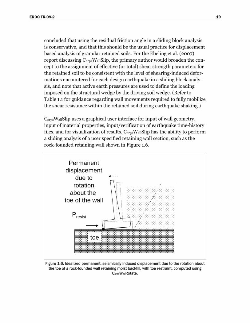
CorpsWallSlip uses a graphical user interface for input of wall geometry, input of material properties, input/verification of earthquake time-history files, and for visualization of results. CorpsWallSlip has the ability to perform a sliding analysis of a user specified retaining wall section, such as the rock-founded retaining wall shown in Figure 1.6.

Presist

Permanentdisplacement

due torotation

about the toe of the wall

toe

Figure 1.6. Idealized permanent, seismically induced displacement due to the rotation about

the toe of a rock-founded wall retaining moist backfill, with toe restraint, computed using CorpsWallRotate.

ERDC TR-09-2 20

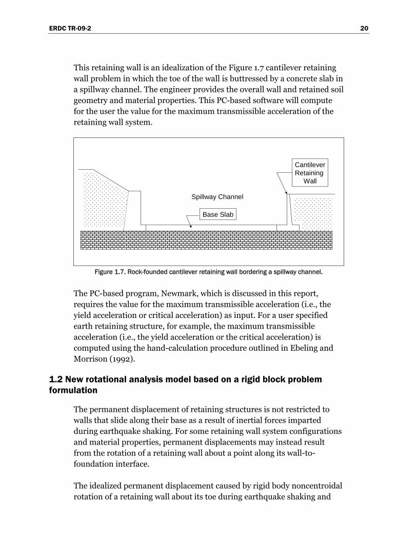
This retaining wall is an idealization of the Figure 1.7 cantilever retaining wall problem in which the toe of the wall is buttressed by a concrete slab in a spillway channel. The engineer provides the overall wall and retained soil geometry and material properties. This PC-based software will compute for the user the value for the maximum transmissible acceleration of the retaining wall system.

Spillway Channel

Base Slab

CantileverRetaining

Wall

Figure 1.7. Rock-founded cantilever retaining wall bordering a spillway channel.

The PC-based program, Newmark, which is discussed in this report, requires the value for the maximum transmissible acceleration (i.e., the yield acceleration or critical acceleration) as input. For a user specified earth retaining structure, for example, the maximum transmissible acceleration (i.e., the yield acceleration or the critical acceleration) is computed using the hand-calculation procedure outlined in Ebeling and Morrison (1992).

1.2 New rotational analysis model based on a rigid block problem formulation

The permanent displacement of retaining structures is not restricted to walls that slide along their base as a result of inertial forces imparted during earthquake shaking. For some retaining wall system configurations and material properties, permanent displacements may instead result from the rotation of a retaining wall about a point along its wall-to-foundation interface.

The idealized permanent displacement caused by rigid body noncentroidal rotation of a retaining wall about its toe during earthquake shaking and

ERDC TR-09-2 21

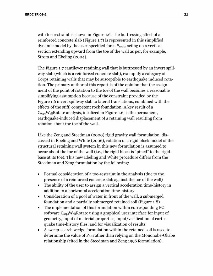
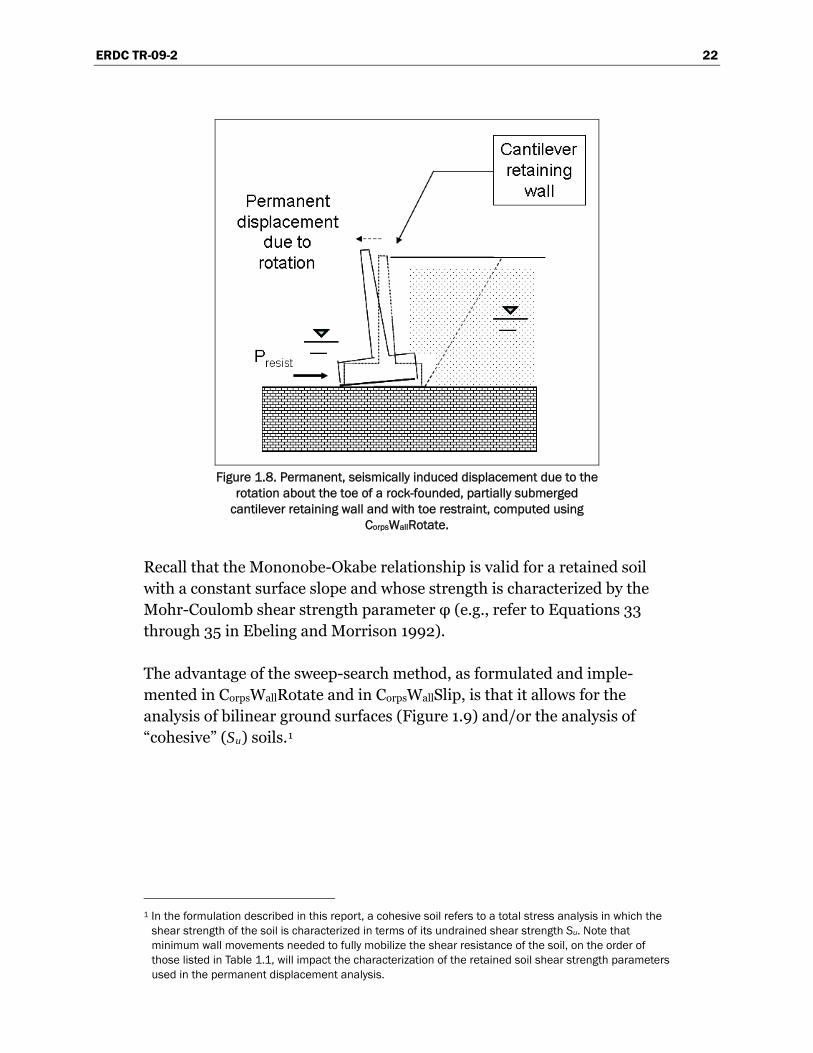
with toe restraint is shown in Figure 1.6. The buttressing effect of a reinforced concrete slab (Figure 1.7) is represented in this simplified dynamic model by the user-specified force Presist acting on a vertical section extending upward from the toe of the wall as per, for example, Strom and Ebeling (2004).

The Figure 1.7 cantilever retaining wall that is buttressed by an invert spill-way slab (which is a reinforced concrete slab), exemplify a category of Corps retaining walls that may be susceptible to earthquake induced rota-tion. The primary author of this report is of the opinion that the assign-ment of the point of rotation to the toe of the wall becomes a reasonable simplifying assumption because of the constraint provided by the Figure 1.6 invert spillway slab to lateral translations, combined with the effects of the stiff, competent rock foundation. A key result of a CorpsWallRotate analysis, idealized in Figure 1.6, is the permanent, earthquake-induced displacement of a retaining wall resulting from rotation about the toe of the wall.

Like the Zeng and Steedman (2000) rigid gravity wall formulation, dis-cussed in Ebeling and White (2006), rotation of a rigid block model of the structural retaining wall system in this new formulation is assumed to occur about the toe of the wall (i.e., the rigid block is “pined” to the rigid base at its toe). This new Ebeling and White procedure differs from the Steedman and Zeng formulation by the following:

• Formal consideration of a toe-restraint in the analysis (due to the presence of a reinforced concrete slab against the toe of the wall)

• The ability of the user to assign a vertical acceleration time-history in addition to a horizontal acceleration time-history

• Consideration of a pool of water in front of the wall, a submerged foundation and a partially submerged retained soil (Figure 1.8)

• The implementation of this formulation within corresponding PC software CorpsWallRotate using a graphical user interface for input of geometry, input of material properties, input/verification of earth-quake time-history files, and for visualization of results

• A sweep-search wedge formulation within the retained soil is used to determine the value of PAE rather than relying on the Mononobe-Okabe relationship (cited in the Steedman and Zeng 1996 formulation).

ERDC TR-09-2 22

Figure 1.8. Permanent, seismically induced displacement due to the

rotation about the toe of a rock-founded, partially submerged cantilever retaining wall and with toe restraint, computed using

CorpsWallRotate.

Recall that the Mononobe-Okabe relationship is valid for a retained soil with a constant surface slope and whose strength is characterized by the Mohr-Coulomb shear strength parameter φ (e.g., refer to Equations 33 through 35 in Ebeling and Morrison 1992).

The advantage of the sweep-search method, as formulated and imple-mented in CorpsWallRotate and in CorpsWallSlip, is that it allows for the analysis of bilinear ground surfaces (Figure 1.9) and/or the analysis of “cohesive” (Su) soils.1

1 In the formulation described in this report, a cohesive soil refers to a total stress analysis in which the

shear strength of the soil is characterized in terms of its undrained shear strength Su. Note that minimum wall movements needed to fully mobilize the shear resistance of the soil, on the order of those listed in Table 1.1, will impact the characterization of the retained soil shear strength parameters used in the permanent displacement analysis.

ERDC TR-09-2 23

AEP

δ

Vertical section through the Heel

H δPAE

Heel+

Heel

AEα

+

θ = 0Vertical section

+ β

K Wh

vK W

W

c' L

N' tan '

Slip Plane

AEα α

P = Pmax

P

ψ

AE

Seismic Iinertia Angle, ψ

hK W

W (1-K )v

tan = ψ Kh1-K v

a = K gh h

a = K gv v

GroundAcceleration+

+

a = K g+

a = K gv v

GroundAcceleration

h h

+

φ

N'

H Level

W

Gravity

a

Center ofh

y

Toe

resistP

TN'

X

Point of Rotation, 0

CG CG

W

Heel

W a

θg I

CGv

g

Figure 1.9. Structural wedge with toe resistance retaining a driving soil wedge with a bilinear moist slope (i.e., no water table) analyzed by effective stress analysis with full mobilization of (c′, φ′) shear resistance

within the backfill.

1.3 The tendency of a retaining wall to slide or to rotate during earthquake shaking

An important difference between the Newmark sliding block method of analysis for earth retaining structures (i.e., the displacement controlled approach that is discussed in Section 1.1.3) and the rotational analysis of a retaining structure modeled as a rigid block is the acceleration imparted to the rigid block. When a rigid block undergoes permanent sliding displace-ment during earthquake shaking, the largest magnitude horizontal accel-eration felt by the rigid block (and the retaining structure contained within the rigid block) is N*g, which is less than the peak value for ground accel-eration. The maximum transmissible acceleration N*g (i.e., the yield accel-eration or critical acceleration) is not the horizontal ground (or, equiva-lently, the rigid base) acceleration representing the earthquake. For a rigid block that undergoes rotation during earthquake shaking, the accelera-tions felt by this rigid block during shaking are those of the ground accel-eration time-history. This is because continuous contact between the rigid block undergoing rotation and the ground is maintained at the point of

ERDC TR-09-2 24

rotation, i.e., the toe in Figure 1.6, during the entire earthquake shaking process.

Thus for a rigid block that undergoes rotation during earthquake shaking, the horizontal acceleration of (rigid) mass center is a function not only of the horizontal ground acceleration but it is also a function of the angular acceleration and the angular velocity during rotation (see Ebeling and White 2006). This differs from the situation of a rigid block that under-goes permanent sliding displacement during earthquake shaking; the largest magnitude horizontal acceleration felt by this rigid block is N*g. Recall that N*g, the maximum transmissible acceleration (i.e., the yield acceleration or critical acceleration) is not the user-defined, horizontal ground (or, equivalently, rigid base) acceleration. Unlike the sliding (rigid) block model, which effectively isolates the sliding block from the shaking base below, the rotating rigid block model continues to transmit horizontal acceleration through the “pin”, located at the toe of the wall, into the wall.

A key step in the evaluation process of the idealized rigid block formula-tions of Ebeling et al. (2007) and of Ebeling and White (2006) for transla-tion and for rotation is the computation of the maximum transmissible acceleration and the computation of threshold value of acceleration corre-sponding to lift-off the base of the wall in rotation. Comparison of these values determines if the wall will tend to slide before it will rotate or visa versa. The lower of the two values dictates the kinematic mechanism for the retaining wall system model. Both of these computational steps are incorporated in both CorpsWallSlip and CorpsWallRotate. The PC-based pro-gram Newmark, described and used in the R&D of this report, does not perform this check nor does it do rotational permanent deformation analyses. For this type of rotational analysis the reader is referred to CorpsWallRotate.

1.4 Seismic design criteria for Corps retaining structures

Current Corps engineering methodology is to evaluate retaining walls for Usual, Unusual and Extreme Loadings. Consideration of earthquake load-ings is part of the design process for Corps earth retaining structures. Engineer Regulation (ER) 1110-2-1806 (Headquarters, U.S. Army Corps of Engineers (HQUSACE) 1995) provides requirements governing the seis-mic design and evaluation of structures located at Corps projects. The engineering procedures outlined in this Corps document are applicable to the analysis of existing, or the design of new earth-retaining structures.

ERDC TR-09-2 25

The Corps regulation for earthquake loadings, ER 1110-2-1806, specifies two project-specific earthquakes, the Operational Basis Earthquake (OBE) and the Maximum Design Earthquake (MDE).

The OBE is an earthquake that can reasonably be expected to occur within the service life of the project, that is, with a 50-percent probability of exceedance during the service life. (This corresponds to a return period of 144 years for a project with a service life of 100 years.) The associated performance requirement is that the project functions with little or no damage, and without interruption of function. The purpose of the OBE is to protect against economic losses from damage or loss of service, and therefore alternative choices of return period for the OBE may be based on economic considerations. The OBE is determined by a Probabilistic Seismic Hazard Analysis (PSHA). The OBE is classified as an Unusual event. Retaining walls are expected to remain serviceable and operable immediately following an OBE earthquake event, or immediately following any earthquake that can reasonably be expected to occur within the service life of the project.

The MDE is the maximum level of ground motion for which a structure is designed or evaluated. The associated performance requirement is that the project performs without catastrophic failure, such as an uncontrolled release of a reservoir, although severe damage or economic loss may be tolerated. For critical features, the MDE is the same as the Maximum Credible Earthquake (MCE). [Section 5(a) and Table B-1 in ER 1110-2-1806 outlines the assessment of the hazard potential classification of Civil Works projects and is related to the consequences of project failure. Critical features are the engineering structures, natural site conditions, or operating equipment and utilities at high hazard projects whose failure during earthquake could result, in loss of life.] For all other features, the MDE shall be selected as a lesser earthquake than the MCE, which pro-vides economical designs meeting appropriate safety standards. The MDE is the maximum level of ground motion for which a structure is designed or evaluated. Although not formally stated in the ER, recent (limited) application to select, normal Corps (non-critical) structures is to assume the MDE is an earthquake that has a 10 percent chance of being exceeded in a 100-year period (or a 975-year return period). The MDE for normal structures is determined by PSHA. For critical structures, the MDE is the Maximum Credible Earthquake (MCE), which is determined by a deter-ministic seismic hazard assessment (DSHA). The MCE is defined as the

ERDC TR-09-2 26

greatest earthquake that can reasonably be expected to be generated on a specific source, on the basis of seismological and geological evidence. Significant damage resulting from an MDE event can be considered as acceptable provided the damaged structure can be repaired and put back in service without risk to life.

Factors of safety and safety requirements for retaining walls subject to seismic loading conditions are provided in EM 1110-2-2100. This super-sedes the stability guidance for retaining walls contained in EM 1110-2-2502 (but not the engineering procedures, which are based on the simplified pseudo-static procedure of analysis).

Factors of safety for sliding and flotation, and the safety provisions related to resultant location and allowable bearing capacity, contained in EM 1110-2-2100 are dependent on:

• Load condition category (usual, unusual, or extreme) • Site information knowledge (well-defined, ordinary, or limited), and • Structure importance (normal, or critical)

EM 1110-2-2100 associates each of the three load condition categories to a range in annual probability (or, equivalently, a range in return period). Additional “structure specific” information related to load condition categories and probabilities are contained in Appendix B of EM 1110-2-2100.

1.5 Axial load capacity of spillway invert slabs

Reinforced concrete slabs provide an important contribution to the overall seismic stability of retaining walls. Figure 1.7 shows, for example, an invert spillway buttressing a cantilever retaining wall that boarders the spillway channel. Key to the seismic performance of this spillway retaining wall is the stabilizing force that the channel invert slab exerts at the toe of this wall. The magnitude of this stabilizing force will depend on the limit state axial load capacity of this invert slab.

Invert slabs can be founded on earth or rock. Types of construction used by the Corps include an “independent block plan” and a “continuous reinforcing plan”. Invert slabs, when loaded axially, can exhibit either short column or long column behavior, with the later referring to slabs

ERDC TR-09-2 27

whose axial capacity is reduced by second-order deformations (i.e., P • Δ effects).

Slab capacity, in terms of axial load versus moment interaction, is deter-mined based on ultimate strength design principles, which can be applied to both unreinforced (plain concrete) and reinforced concrete invert slab sections. Influences from the subgrade reaction, slab dead load, and axial load eccentricity, when considered in a second-order analysis, suggest the axial load capacity can be based on a short column design with second-order displacements resulting from P • Δ effects having little if any effect on column axial load capacity, according to the Strom and Ebeling (2004).

The axial load resistance Presist, provided by the Figure 1.7 invert slab, is illustrated in Figure 1.6. Limited investigations, by Strom and Ebeling (2004), based on the Corps minimum thickness for invert slabs con-structed on rock and earth, and for both continuous reinforcing plans and independent block plans, indicate the limit state axial load capacity, or ultimate axial load resistance of the slab (Presist) may be on the order of:

• 120 kips per foot width of slab for a 1.0 foot thick invert slab on rock • 240 kips per foot width of slab for a 2.0 foot thick invert slab on soil

The above values are valid for both anchored and unanchored invert slabs, and for the minimum contraction joint spacings typically found on Corps projects. However, a site-specific evaluation of the limiting axial resisting force resulting from the buttressing effect of the type of slab on the toe of a retaining wall is required. Refer to Strom and Ebeling (2004) for a simpli-fied engineering methodology for the assessment of Presist for all types of slabs buttressing all types of retaining structures, including the Figure 1.7 invert spillway slab.

1.6 Background and research objective

EM 1110-2-2502, Retaining and Flood Walls, gives engineering procedures that are currently being used by District Engineers in their initial assess-ment of seismic wall performance of existing earth retaining structures and the (preliminary) sizing of new retaining structures. The engineering procedures given in EM 1110-2-2502 for retaining walls make extensive use of the simplified pseudo-static procedure of analysis of earth retaining structures and express wall performance criteria in terms of computed factors of safety against sliding and bearing failure, and base area in

ERDC TR-09-2 28

compression. The simplified pseudo-static procedure of analysis makes it difficult to interpret the actual wall performance for Corps projects subjected to “strong” design ground motions because of simplifications made in the procedure of analysis. In a pseudo-static analysis, an over-simplification occurs when the engineer is forced to render the complex, horizontal and vertical earthquake acceleration time-history events to constant values of accelerations and to assume a constant direction for each. These constant values are denoted as the pseudo-static acceleration coefficients in the horizontal and vertical directions (refer to Section 1.1.1 of this report). The engineer is also required to assume a constant direc-tion for each of these components. An acceleration time-history, in actuality, varies both in magnitude and in direction with time.

The simplified pseudo-static procedure does not allow for interpretation of actual wall performance by District Engineers. Intense shaking imparted by the OBE and MCE design events makes the interpretation of the simpli-fied procedure of analysis even more difficult. The more important questions for the wall are whether the wall slides into the spillway basin, or rotates into the spillway basin, or even tips over onto its side during the earthquake event. The simplified pseudo-static procedure of analysis is not capable of answering these questions. The answers depend on the magni-tude of the pseudo-static coefficient used in the calculations compared to the magnitude of the peak values for the acceleration pulses as well as the number and duration of these strong shaking acceleration pulses in the design earthquake event time-history. When considering both horizontal and vertical accelerations, the resulting wall response is further compli-cated by the time-history of phasing between the pulses of horizontal and vertical accelerations. Only the permanent wall sliding displacement/wall rotation method of time-history analysis can answer these questions. Again, wall displacements will influence the seismic earth pressure forces imparted on the wall by the retained soil.

Formal consideration of the permanent seismic wall displacement in the seismic design process for Corps-type retaining structures is given in Ebeling and Morrison (1992). The key aspect of the engineering approach presented in this Corps document is that simplified procedures for com-puting the seismically induced earth loads on retaining structures are also dependent upon the amount of permanent wall displacement that is expected to occur for each specified design earthquake. The Ebeling and Morrison simplified engineering procedures for Corps retaining structures

ERDC TR-09-2 29

are geared toward hand calculations. The engineering formulation and corresponding PC software CorpsWallSlip (Ebeling et al. 2007) extend these simplified procedures to walls that slide during earthquake shaking and make possible the use of acceleration time-histories in the Corps design/ analysis process when time-histories are made available on Corps projects. CorpsWallSlip may be used to predict permanent seismically induced translational displacements of walls retaining backfill, with or without a toe restraint. It is particularly applicable to rock-founded L-walls and T-walls (i.e., cantilever retaining walls) which border spillway channels (Figure 1.7). The PC software Newmark discussed in this report may also be used to perform the same permanent (translational) deformation analysis as CorpsWallSlip, but does require the additional step of the user computing and providing as input the maximum transmissible accelera-tion (i.e., the yield acceleration or the critical acceleration).

The software Newmark is also capable of performing regression analyses on multiple horizontal acceleration time histories for up to three pre-set (mathematical) formulations, for the purpose of developing simplified non-dimensional (simplified) permanent displacement relationships for use in a Simplified Sliding Block Analysis of a structural system. The main purpose of developing the software Newmark in this R&D effort is to facil-itate the processing of multiple rock acceleration time histories and to perform a statistical analysis of the computed permanent displacements for multiple, user-defined critical accelerations. From these data, simpli-fied permanent displacement relationships are derived, concluding in the selection of recommended relationships. These resulting simplified sliding block relationships based for rock-founded structures are based on data from rock acceleration time histories and will be implemented within CorpsWallSlip (Ebeling et al. 2007) for Corps earth retaining structures and within CorpsDamSlip (under development by Ebeling and Chase) for Corps rock-founded gravity dams.

1.7 Organization of report

Chapter 2 describes the numerical method implemented in the software Newmark for performing a translational (i.e., sliding) block analysis of a structural system model of e.g., a retaining structure or a rock-founded gravity dam, etc. The formulation used computes the permanent sliding displacement response of a structural system to an earthquake accelera-tion time-history via a Complete Time-History Analysis.

ERDC TR-09-2 30

Chapter 3 describes three formulations used for developing simplified non-dimensional (simplified) permanent displacement relationships for use in a Simplified Sliding Block Analysis of a structural system. The regression analyses result in mean estimates and together with their standard error terms, also determine the 68 percent prediction intervals and 95 percent probability of non-exceedance upper bound estimates to seismically induced permanent (translational) displacement at the end of earthquake shaking.

Chapter 4 discusses the selection process and the characteristics of each of the 122 sets of baseline corrected “rock” acceleration time histories used in the regression analysis and the results of these analyses for the three sim-plified permanent (translational) displacement relationships introduced in Chapter 3.

Chapter 5 describes key aspects of the visual modeler and visual post-processor Newmark. Specifically, a description of the graphical user inter-face for input of value(s) of critical acceleration (i.e., the maximum trans-missible acceleration or the yield acceleration), input/verification of earth-quake time-history files, and for visualization of results is presented to make the user familiar with its operation.

Chapter 6 presents a summary of the recommended simplified permanent (translational) deformation relationships developed during the course of this research, conclusions and recommendations for additional research.

Appendix A is a listing and description of the Newmark ASCII input data file (file name: Newmark.in).

Appendix B is a listing and description of Newmark ASCII Data Output Files.

ERDC TR-09-2 31

2 Translational Block Analysis of a Rock Founded Structural Model

2.1 Introduction

This chapter describes an engineering formulation developed for com-puting the permanent translational response of the Corps rock founded hydraulic structures (e.g., an earth retaining structure, a concrete gravity dam, etc.) to earthquake ground motions. The resulting engineering formulation is implemented within corresponding PC software Newmark using a graphical user interface for input/verification of earthquake time-history files, input of the hydraulic structures critical acceleration (i.e., maximum transmissible acceleration or yield acceleration) and for visual-ization of results. The PC software Newmark was developed to perform an analysis of the permanent sliding displacement response of a rigid block model of a structural section to a user specified earthquake acceleration time-history via a Complete Time-History Analysis. The Complete Time-History method of analysis is discussed first in this chapter. (Key aspects of the Visual Modeler, the PC-based Graphical User Interface (GUI) to Newmark are described in Chapter 5.) The main purpose of developing the software Newmark in this R&D effort is to facilitate the processing of multiple rock acceleration time histories and perform a statistical analysis (using the procedures discussed in Chapter 3) of the computed permanent displacements for multiple, user-defined critical accelerations. From this data, simplified permanent displacement relationships are derived (dis-cussed in Chapter 4), with recommended relationships summarized in Chapter 6. These resulting simplified sliding block relationships for rock-founded structures will be implemented within CorpsWallSlip (Ebeling et al. 2007) for earth retaining structures and within CorpsDamSlip (under devel-opment by Ebeling and Chase) for Corps rock-founded gravity dams.

The software Newmark may also be used to compute the permanent (translational) displacement of a rigid block model for a single acceleration time-history. Besides an acceleration time-history, a user specified value for the structure’s critical acceleration (i.e., maximum transmissible accel-eration or yield acceleration) is required. Recall that the value for the criti-cal acceleration (i.e., N*g; the maximum transmissible acceleration in Ebeling and Morrison (1992) terminology for retaining walls) is the

ERDC TR-09-2 32

horizontal acceleration imparted to the rigid body model, that will nomi-nally exceed the shear resistance provided by the foundation along (or immediately below) the interface between the base of the rigid body and the foundation (refer to Figure 1.4). Earth retaining structures and earthen slope/embankments were discussed in Chapter 1 with regard to (Newmark) permanent displacement based sliding block analysis resulting from earthquake shaking. Hand calculations of the critical acceleration (i.e., the maximum transmissible acceleration or the yield acceleration) for a particular earth retaining structure are described in Ebeling and Morrison (1992). Alternatively, CorpsWallSlip (Ebeling et al. 2007) may be used to automatically compute the rock-founded earth retaining struc-ture’s critical acceleration using the user defined geometry, retained soil and rock foundation properties (as well as the value for the structure’s critical acceleration). Several popular slope stability software programs have the capability to compute the critical acceleration for an earthen slope/embankment. The computation of the critical acceleration is done prior to executing Newmark, when evaluating a structure for its per-manent displacement to a single user-specified acceleration time-history. (Note that when using the software Newmark in this fashion for a slope/ embankment, the acceleration time-history used is likely to an accelera-tion time-history recorded on a soil site.)

2.2 Time-history of permanent structural displacement

Earthquake shaking of the rock foundation is represented by time histories of acceleration in the translational block formulation implemented in pro-gram Newmark for the Complete Time-History Analysis.1 Since the ground acceleration varies with time, let the horizontal ground acceleration be represented by variable fraction A times the constant acceleration of gravity g in Figure 1.5. Recall that the integral of the acceleration time-history is equal to the velocity time-history and the integral of velocity is displacement (i.e., the permanent structural displacement in this case). For a “rigid block” subjected to an acceleratioof value larger than the Figure 1.5 maximum transmissible acceleration, labeled N*g in this figure, the rigid block will displace. When this occurs over several time steps, the total permanent displacement of a sliding block relative to the base (i.e., the rock foundation) is the sum of the increments of displacement occurring during a number of individual

n

1 Baseline-corrected, horizontal acceleration time histories are to be used to represent the earthquake

ground motions in program Newmark.

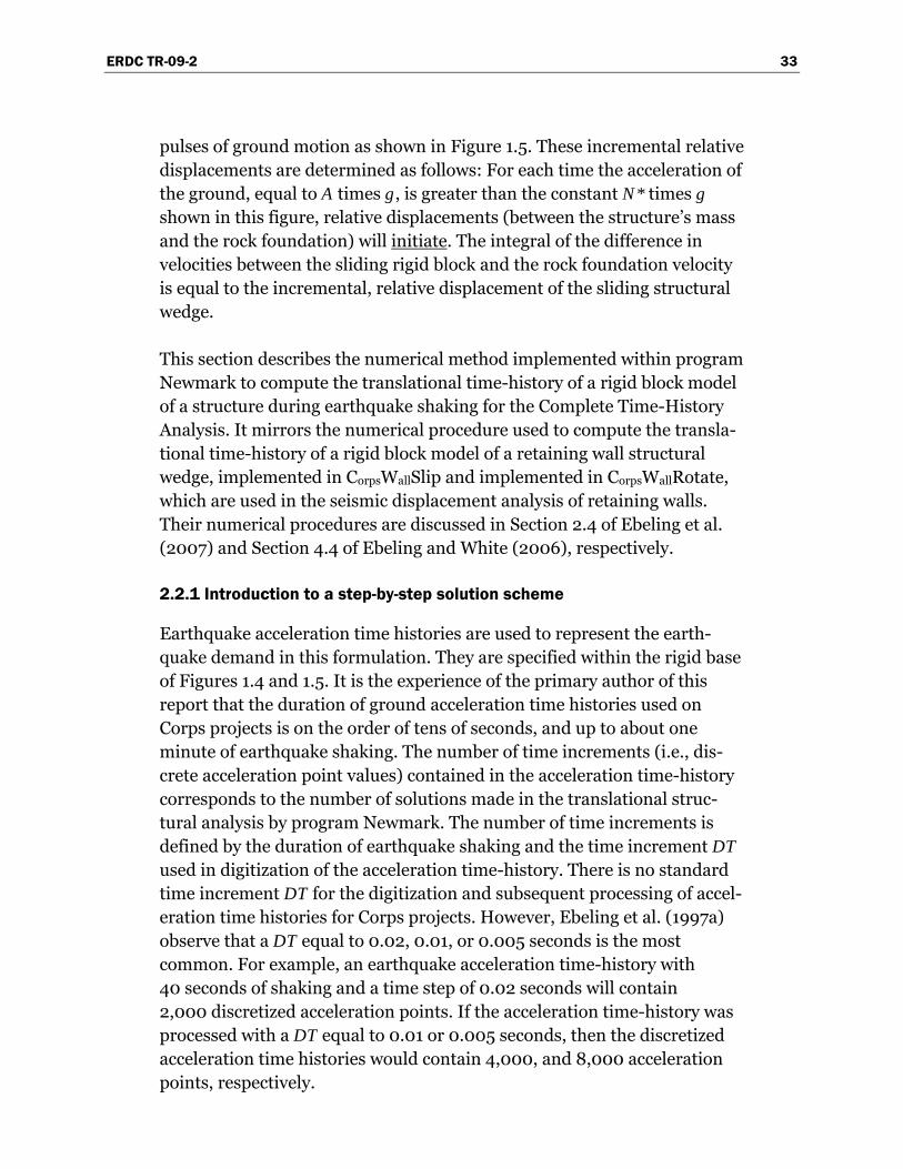
ERDC TR-09-2 33

pulses of ground motion as shown in Figure 1.5. These incremental relatdisplacements are determined as follows: For each time the acceleration of the ground, equal to A times g, is greater than the constant N* times g shown in this figure, relative displacements (between the structure’s masand the rock foundation) will

ive

s initiate. The integral of the difference in

velocities between the sliding rigid block and the rock foundation velocitis equal to the incremental, relative displacement of th

y e sliding structural

wedge.

l

la-

e,

et al. (2007) and Section 4.4 of Ebeling and White (2006), respectively.

2.2.1 Introduction to a step-by-step solution scheme

ase

y

-97a)

h

ories would contain 4,000, and 8,000 acceleration points, respectively.

This section describes the numerical method implemented within programNewmark to compute the translational time-history of a rigid block modeof a structure during earthquake shaking for the Complete Time-History Analysis. It mirrors the numerical procedure used to compute the transtional time-history of a rigid block model of a retaining wall structural wedge, implemented in CorpsWallSlip and implemented in CorpsWallRotatwhich are used in the seismic displacement analysis of retaining walls. Their numerical procedures are discussed in Section 2.4 of Ebeling

Earthquake acceleration time histories are used to represent the earth-quake demand in this formulation. They are specified within the rigid bof Figures 1.4 and 1.5. It is the experience of the primary author of this report that the duration of ground acceleration time histories used on Corps projects is on the order of tens of seconds, and up to about one minute of earthquake shaking. The number of time increments (i.e., dis-crete acceleration point values) contained in the acceleration time-historcorresponds to the number of solutions made in the translational struc-tural analysis by program Newmark. The number of time increments is defined by the duration of earthquake shaking and the time increment DTused in digitization of the acceleration time-history. There is no standard time increment DT for the digitization and subsequent processing of acceleration time histories for Corps projects. However, Ebeling et al. (19observe that a DT equal to 0.02, 0.01, or 0.005 seconds is the most common. For example, an earthquake acceleration time-history wit40 seconds of shaking and a time step of 0.02 seconds will contain 2,000 discretized acceleration points. If the acceleration time-history wasprocessed with a DT equal to 0.01 or 0.005 seconds, then the discretized acceleration time hist

ERDC TR-09-2 34

A step-by-step solution scheme is followed in order to obtain the struc-ture’s permanent translational relative velocity, relV, and displacement, relD, in the time domain by program Newmark. An overview of the char-acteristics of this numerical formulation is depicted in Figure 2.1. A key feature of the numerical formulation used is the assumption of a linear variation in relative acceleration relA over time step DT, from time ti to time ti+1. Values of the user-provided ground acceleration (specified within the rigid base model) are compared against the critical acceleration (i.e., maximum transmissible acceleration or yield acceleration) value at each time step.

T

DT

RelativeAcceleration(Linear)

Velocity(Quadratic)

Relative

(Cubic)DisplacementRelative

Note: Postive relV0 value.

relA0

relV0

relD0

0

0

0 0

0

0

at incrementaltime

T

relA1

relV1

relD1

relA = relA0

(relA1-relA0)T DT

relV = relV0

relD = relD0+ ( ) relV0

T ( ) relA0

DT ( ) (relA1-relA0)T

2

2

T+ ( ) relA0

2T

( ) (relA1-relA0)T6 DT

2

3

ti ti+1

+

+

+

+

( )

Figure 2.1. Complete equations for relative motions over time increment DT based on linearly

varying acceleration.

ERDC TR-09-2 35

This idealized figure assumes that the structure is undergoing positive relative acceleration (i.e., the value for acceleration of the ground is greater than the value of critical acceleration, positive relative velocity, and posi-tive (permanent) displacement at time ti, which continues through time ti+1). The relative acceleration values relA0 and relA1 are equal to the dif-

ference between the horizontal ground acceleration value minus the con-stant value of critical acceleration at times ti and ti+1, respectively, and are assumed positive at both time steps. (Other cases will be considered later.) The idealized figure also assumes that the relative acceleration increases in magnitude over this time step DT, as depicted in this figure. The relative velocity is computed by integrating the relative acceleration during each segment of structural translation.

when relV > 0 (2.1) t

relV relA dt= ∫0

or

when Equation 2.1 gives relV less than 0 (2.2) relV = 0

So, for a linear variation in relative acceleration over time step DT, the relative velocity, relV, is a quadratic relationship. Note that program Newmark assumes that the structure cannot slide backwards (i.e., it is impeded by the retained soil for an earth retaining structure or by the pool for a gravity dam, which is expressed by Equation 2.2. Similarly, with the permanent relative displacement of the structure being the integration of the relative velocity, the relative displacement of the structure is a cubic relationship, as listed in Figure 2.1. The permanent relative displacement of the structure is the integration of the relative velocity

(2.3) t

relD relV dt= ∫0

This series of computations using relative accelerations and Equations 2.1 through 2.3 are repeated for each sequence of structural translations that occurs for the duration of earthquake shaking. The experience of the pri-mary author of this report is that, when the acceleration time histories used as input to program Newmark are based on previously recorded earthquake events (a typical scenario), the permanent displacement occurs

ERDC TR-09-2 36

during several, separate pulses occurring throughout the duration of shaking.

In Figure 2.1, the value for relative acceleration relA, relative velocity relV and (permanent structural) relative displacement relD at any point in time Δt after ti and before time ti+1 are given by the linear, quadratic and cubic relationships contained on the right-hand side of these three figures (with Δt less than or equal to DT).

Recall that during sliding, the acceleration felt by the structure equals the maximum transmissible acceleration. Thus, the sliding (rigid) block model effectively isolates the sliding block from the shaking (rigid) base below.

2.2.2 Positive relative accelerations relA0 and relA1 at times ti and ti+1

Expanding on the details of the computations for the numerical formula-tion depicted in Figure 2.1, the computation of the relative acceleration, relA, relative velocity, relV, and relative displacement, relD, at time ti+1 are made as follows: values for relA, relV, relD, at time ti are known from the previous computation step in the step-by-step solution scheme. The value for relA at time ti+1 (designated relA1 in the figure) is computed as the

difference between horizontal ground acceleration minus the constant value of critical acceleration. Referring to Figure 2.2, the relative velocity at time ti+1 (designated relV1) is computed from the value for relative velocity at time ti (designated relV0) plus the positive area under the linear

relative acceleration relationship over the time step DT, designated Areaa in this figure. By the trapezoidal rule, relV1 at time ti+1 is

(DTrelV relV relA relA= + • +1 0 0

2)1 (2.4)

with the values for relV0 and relA0 now being known values that were

computed in the previous solution step. Note that the structure is in motion at time ti, as reflected by a positive value for relative velocity (designated relV0 in Figure 2.2). Similarly, the permanent relative struc-tural displacement at time ti+1 (designated relD1) is computed from the value for relative displacement at time ti (designated relD0) plus the

positive area under the quadratic relative velocity relationship over the time step DT, designated Areav in this figure. For this linear acceleration method, relD1 at time ti+1 is

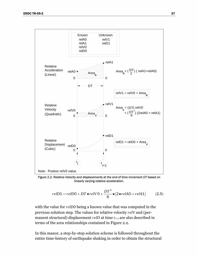
ERDC TR-09-2 37

DT

RelativeAcceleration(Linear)

Velocity(Quadratic)

Relative

(Cubic)DisplacementRelative

Note: Postive relV0 value.

relA0

relV0

relD0

0

0

0 0

0

0

relA1

relV1

relD1

relD1 = relD0 + Area

DT2

ti ti+1

Areaa

Areav

Known UnknownrelA0relA1relV0relD0

relV1relD1

aArea = ( ) ( relA1+relA0)

relV1 = relV0 + Areaa

Area = ( ) relV0DT+ ( ) (2relA0 + relA1)DT

62

v

v

Figure 2.2. Relative Velocity and displacements at the end of time increment DT based on

linearly varying relative acceleration.

( )DTrelD relD DT relV relA relA= + • + • • +

2

1 0 0 2 06

1 (2.5)

with the value for relD0 being a known value that was computed in the

previous solution step. The values for relative velocity relV and (per-manent structural) displacement relD at time ti+1 are also described in terms of the area relationships contained in Figure 2.2.

In this manor, a step-by-step solution scheme is followed throughout the entire time-history of earthquake shaking in order to obtain the structural

ERDC TR-09-2 38

velocity, relV, and relative displacement, relD, at each increment in time in the Figure 2.2 case of positive values for relA at times ti and ti+1.

In summary, Figure 2.2 outlines a numerical procedure to obtain values for relative velocity and for relative displacement at time ti+1 in situations for which values of relative acceleration relA at times ti and ti+1 are both positive.

However, there are three other situations that can arise during the step-by-step solution:

• The case of a negative value for relA at time ti and a positive value for relA at time ti+1

• The case of structure decelerating over the entire time step DT for which the values of relA are negative at both times ti and ti+1

• The case of a positive value for relA at time ti and a negative value for relA at time ti+1.

In all four cases, the assumption of linear relative acceleration over time step DT is made and the basic concept of integrating positive areas above and/or negative areas below the time-line of relative acceleration relA to obtain the change in relative velocity relV and then, in turn, the integration of positive and/or negative areas above and/or below the time-line of relV to obtain the change in relative displacement relD is used to determine the values for relV and relD, respectively, at time ti+1. These three additional step-by-step solutions will be discussed next. Note the frequent use of the trapezoidal rule for relV and the linear acceleration method for relD in the solution processes to be described.

2.2.3 Positive relative acceleration relA0 at time ti and negative relative acceleration relA1 at ti+1

Next, consider a structure in motion (i.e., with a positive value for relV) at time ti but with the Figure 2.3 case of a negative value for relA0 computed at time step ti and positive value for relA1 computed at the next time step

of ti+1.1 The first step is to determine the time instant [ti plus lhsDT] at which the relative acceleration relA is equal to zero, as labeled in the figure. By linear interpolation, this time increment lhsDT is

1 Note the assumption of a linear variation in relative acceleration over the time step DT in Figure 2.3.

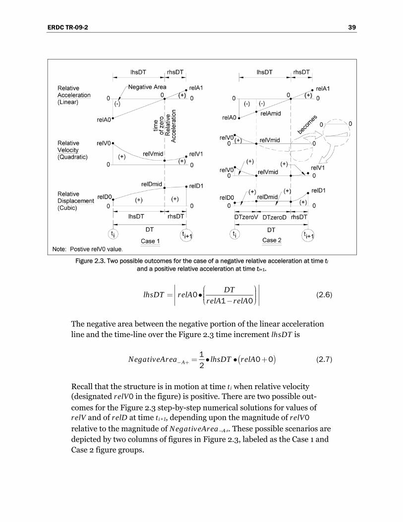
ERDC TR-09-2 39

Figure 2.3. Two possible outcomes for the case of a negative relative acceleration at time ti

and a positive relative acceleration at time ti+1.

DTlhsDT relA

relA relA

⎛ ⎞⎟⎜= • ⎟⎜ ⎟⎜⎝ ⎠−0

1 0 (2.6)

The negative area between the negative portion of the linear acceleration line and the time-line over the Figure 2.3 time increment lhsDT is

( )ANegativeArea lhsDT relA− + = • • +1 0 02

(2.7)

Recall that the structure is in motion at time ti when relative velocity (designated relV0 in the figure) is positive. There are two possible out-

comes for the Figure 2.3 step-by-step numerical solutions for values of relV and of relD at time ti+1, depending upon the magnitude of relV0

relative to the magnitude of NegativeArea−Α+. These possible scenarios are depicted by two columns of figures in Figure 2.3, labeled as the Case 1 and Case 2 figure groups.

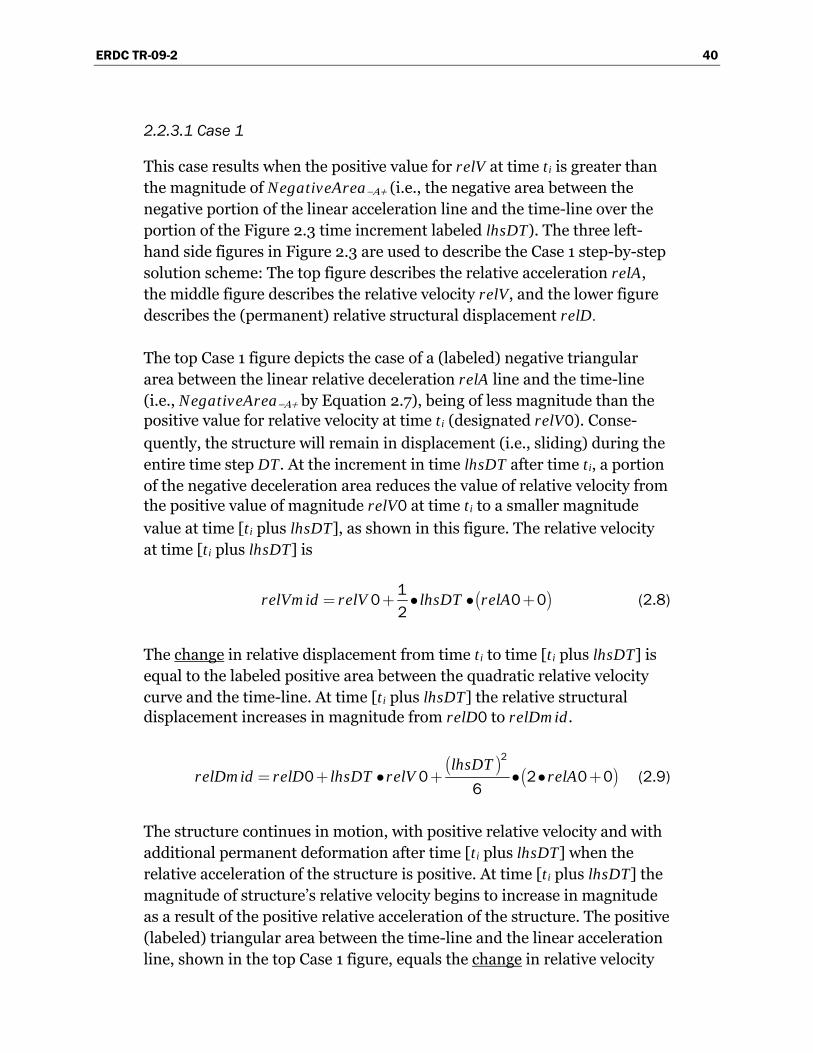
ERDC TR-09-2 40

2.2.3.1 Case 1

This case results when the positive value for relV at time ti is greater than the magnitude of NegativeArea−Α+ (i.e., the negative area between the negative portion of the linear acceleration line and the time-line over the portion of the Figure 2.3 time increment labeled lhsDT). The three left-hand side figures in Figure 2.3 are used to describe the Case 1 step-by-step solution scheme: The top figure describes the relative acceleration relA, the middle figure describes the relative velocity relV, and the lower figure describes the (permanent) relative structural displacement relD.

The top Case 1 figure depicts the case of a (labeled) negative triangular area between the linear relative deceleration relA line and the time-line (i.e., NegativeArea−Α+ by Equation 2.7), being of less magnitude than the positive value for relative velocity at time ti (designated relV0). Conse-

quently, the structure will remain in displacement (i.e., sliding) during the entire time step DT. At the increment in time lhsDT after time ti, a portion of the negative deceleration area reduces the value of relative velocity from the positive value of magnitude relV0 at time ti to a smaller magnitude

value at time [ti plus lhsDT], as shown in this figure. The relative velocity at time [ti plus lhsDT] is

(relVmid relV lhsDT relA= + • • +102

)0 0 (2.8)

The change in relative displacement from time ti to time [ti plus lhsDT] is equal to the labeled positive area between the quadratic relative velocity curve and the time-line. At time [ti plus lhsDT] the relative structural displacement increases in magnitude from relD0 to relDmid.

( ) ( )lhsDT

relDmid relD lhsDT relV relA= + • + • • +2

0 0 26

0 0 (2.9)

The structure continues in motion, with positive relative velocity and with additional permanent deformation after time [ti plus lhsDT] when the relative acceleration of the structure is positive. At time [ti plus lhsDT] the magnitude of structure’s relative velocity begins to increase in magnitude as a result of the positive relative acceleration of the structure. The positive (labeled) triangular area between the time-line and the linear acceleration line, shown in the top Case 1 figure, equals the change in relative velocity

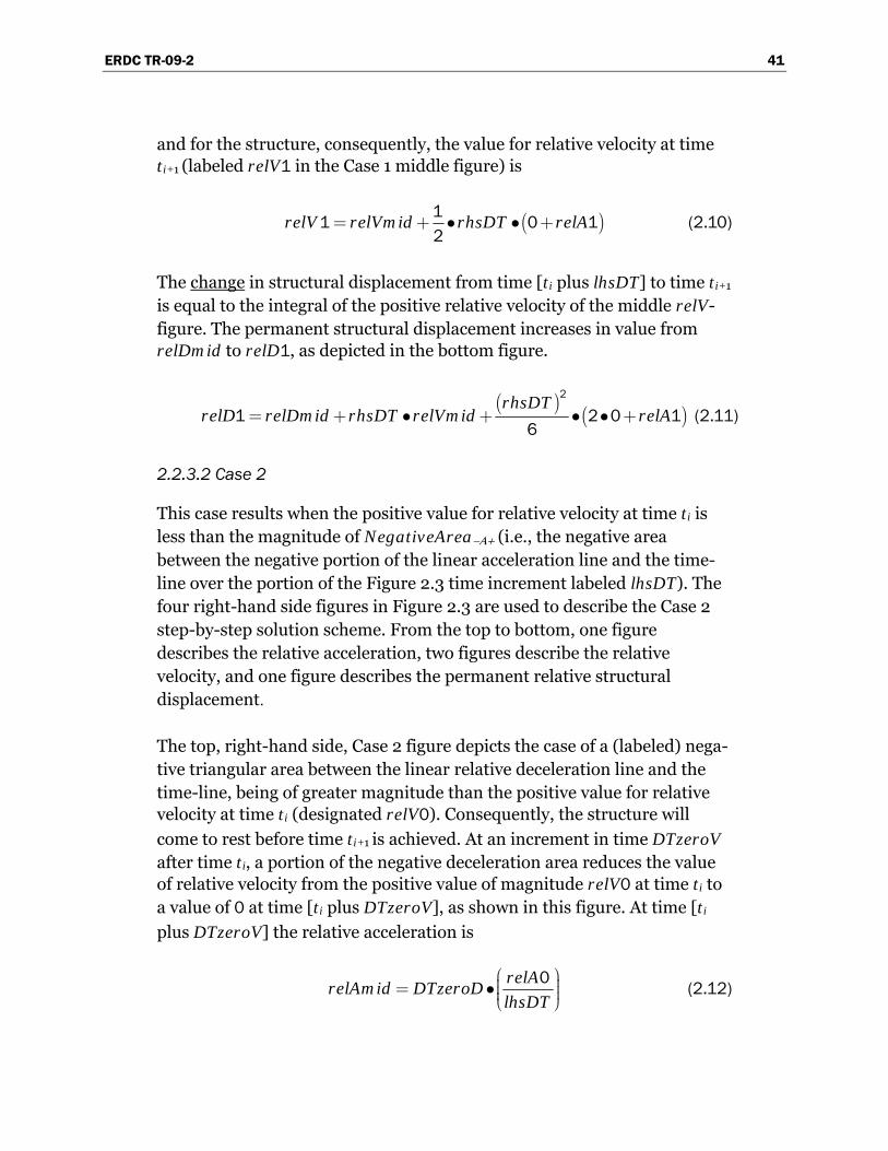
ERDC TR-09-2 41

and for the structure, consequently, the value for relative velocity at time ti+1 (labeled relV1 in the Case 1 middle figure) is

( )relV relVmid rhsDT relA= + • • +112

0 1 (2.10)

The change in structural displacement from time [ti plus lhsDT] to time ti+1

is equal to the integral of the positive relative velocity of the middle relV-figure. The permanent structural displacement increases in value from relDmid to relD1, as depicted in the bottom figure.

( ) ( )rhsDT

relD relDmid rhsDT relVmid relA= + • + • • +2

1 26

0 1 (2.11)

2.2.3.2 Case 2

This case results when the positive value for relative velocity at time ti is less than the magnitude of NegativeArea−Α+ (i.e., the negative area between the negative portion of the linear acceleration line and the time-line over the portion of the Figure 2.3 time increment labeled lhsDT). The four right-hand side figures in Figure 2.3 are used to describe the Case 2 step-by-step solution scheme. From the top to bottom, one figure describes the relative acceleration, two figures describe the relative velocity, and one figure describes the permanent relative structural displacement.

The top, right-hand side, Case 2 figure depicts the case of a (labeled) nega-tive triangular area between the linear relative deceleration line and the time-line, being of greater magnitude than the positive value for relative velocity at time ti (designated relV0). Consequently, the structure will

come to rest before time ti+1 is achieved. At an increment in time DTzeroV after time ti, a portion of the negative deceleration area reduces the value of relative velocity from the positive value of magnitude relV0 at time ti to a value of 0 at time [ti plus DTzeroV], as shown in this figure. At time [ti

plus DTzeroV] the relative acceleration is

relArelAmid DTzeroD

lhsDT

⎛ ⎞⎟⎜= • ⎟⎜ ⎟⎜⎝ ⎠0 (2.12)

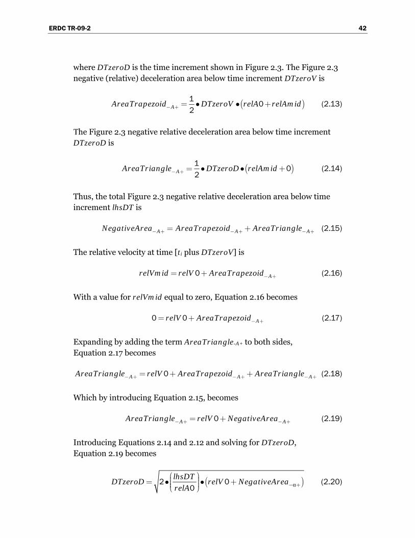
ERDC TR-09-2 42

where DTzeroD is the time increment shown in Figure 2.3. Τhe Figure 2.3 negative (relative) deceleration area below time increment DTzeroV is

( )AAreaTrapezoid DTzeroV relA relAmid− + = • • +1 02

(2.13)

Τhe Figure 2.3 negative relative deceleration area below time increment DTzeroD is

(AAreaTriangle DTzeroD relAmid− + = • • +1 02

) (2.14)

Thus, the total Figure 2.3 negative relative deceleration area below time increment lhsDT is

A A ANegativeArea AreaTrapezoid AreaTriangle− + − + − += + (2.15)

The relative velocity at time [ti plus DTzeroV] is

ArelVmid relV AreaTrapezoid− += +0 (2.16)

With a value for relVmid equal to zero, Equation 2.16 becomes

ArelV AreaTrapezoid− += +0 0 (2.17)

Expanding by adding the term AreaTriangle-A+ to both sides, Equation 2.17 becomes

A A AAreaTriangle relV AreaTrapezoid AreaTriangle− + − + − += + +0 (2.18)

Which by introducing Equation 2.15, becomes

A AAreaTriangle relV NegativeArea− + − += +0 (2.19)

Introducing Equations 2.14 and 2.12 and solving for DTzeroD, Equation 2.19 becomes

( )αlhsDT

DTzeroD relV NegativeArearelA − +

⎛ ⎞⎟⎜= • • +⎟⎜ ⎟⎜⎝ ⎠2 0

0 (2.20)

ERDC TR-09-2 43

Recognizing the time increment lhsDT is equivalent to

(2.21) lhsDT DTzeroV DTzeroD= +

and by introducing Equations 2.21 and 2.13 into Equation 2.20 and solving for DTzeroV,

( )AlhsDT

DTzeroV lhsDT relV NegativeArearelA − +

⎛ ⎞⎟⎜= − • • +⎟⎜ ⎟⎜⎝ ⎠2 0

0 (2.22)

The change in relative displacement from time ti to time [ti plus DTzeroV] is equal to the labeled positive area between the quadratic relative velocity curve and the time-line. At time [ti plus DTzeroV] the structural displace-ment increases in magnitude from relD0 to relDmid. The relative velocity

at time [ti plus DTzeroV], expressed in terms of DTzeroV, is

( )relVmid relV DTzeroV relA relAmid= + • • +10 02

(2.23)

with the relative acceleration at time [ti plus DTzeroV] equal to

relA relArelAmid relA DTzeroV

DT

⎛ ⎞− ⎟⎜= + •⎟⎜ ⎟⎜⎝ ⎠1 00 (2.24)

The change in relative displacement from time ti to time [ti plus DTzeroV] is equal to the labeled positive area between the quadratic relative velocity curve and the time-line. At time [ti plus DTzeroV] the structural displace-ment increases in magnitude from relD0 to relDmid.

( ) ( )

relDmid relD DTzeroV relV

DTzeroVrelA relAmid

= + •

+ • • +2

0 0

2 06

(2.25)

The structure remains at rest with zero relative velocity and with no addi-tional permanent relative displacement from time [ti plus DTzeroV] until time [ti plus lhsDT] when the relative acceleration of the structure begins (again). At time [ti plus lhsDT] the structure begins to develop further permanent displacement as a result of the positive relative reacceleration of the structure. The positive (labeled) triangular area between the

ERDC TR-09-2 44

time-line and the linear relative acceleration line, shown in the right-hand side of the top figure, equals the change in relative velocity and with the structure at rest , consequently, the value for relative velocity at time ti+1 (labeled relV1 in the lower relative velocity figure) is

( )relV rhsDT relA= • • +11 02

1 (2.26)


is equal to the integral of the positive relative velocity, as depicted in the middle two, right-hand side relV-figures. The top relV figure is a computa-tional figure, and the bottom relV figure is the relV curve-shift figure that properly accounts for zero structural relative velocity over time increment DTzeroD, with an insert detailed, curve-shift figure for relV shown of this computational relV figure in Figure 2.3. The permanent relative structural displacement increases in value from relDmid to relD1, as depicted in the

bottom figure.

( ) ( )rhsDT

relD relDmid rhsDT relA= + • + • • +2

1 0 26

0 1 (2.27)

2.2.4 Negative relative accelerations relA0 and relA1 at times ti and ti+1

Next, consider a structure in motion (i.e., with a positive value for relative velocity) at time ti but with the Figure 2.4 case of a negative values for relative acceleration computed at time steps ti and ti+1.1

The first step is to determine if the structure, which is in motion at time ti, comes to rest during the time step DT.

The negative area between the negative portion of the linear acceleration line and the time-line over the Figure 2.4 time increment DT is

(ANegativeArea DT relA relA− − = • • +1 02

)1

(2.28)

1 Again, note the assumption of a linear variation in relative acceleration over the time step DT shown in

Figure 2.4.

ERDC TR-09-2 45

Figure 2.4. Two possible outcomes for the case of negative relative accelerations at times ti and ti+1.

There are two possible outcomes for the Figure 2.4 step-by-step numerical solution for relative velocity and relative displacement at time ti+1, depend-ing upon the magnitude of relV0 relative to the magnitude of Equa-

tion 2.28 NegativeArea−Α− . These possible scenarios are depicted by two columns of figures in Figure 2.4, labeled as Case 1 and Case 2 figure groups.

2.2.4.1 Case 1

This case results when the positive value for relative velocity at time ti is greater than the magnitude of NegativeArea−Α− (i.e., the negative area between the negative portion of the linear acceleration line and the time-line over the Figure 2.4 time step DT). The three left-hand side figures in Figure 2.4 are used to describe the Case 1 step-by-step solution scheme: The top figure describes the relative acceleration, the middle figure describes the relative velocity, and the lower figure describes the permanent relative structural displacement.

ERDC TR-09-2 46

The top Case 1 figure depicts the case of a (labeled) negative area between the linear relative deceleration line and the time-line (i.e., NegativeArea−Α− by Equation 2.28), being of less magnitude than the positive value for relative velocity at time ti (designated relV0). Conse-

quently, the structure will remain in motion during the entire time step DT. At the time step DT after time ti, the negative deceleration area reduces the value of relative velocity from the positive value of magnitude relV0 at time ti to a smaller magnitude value at time [ti plus DT], as shown

in this figure. The relative velocity at time [ti plus DT] is

(relV relV DT relA relV= + • • +11 0 02

)1 (2.29)

The change in relative displacement from time ti to time [ti plus DT] is equal to the labeled positive area between the quadratic relative velocity curve and the time-line. At time [ti plus DT] the structural displacement increases in magnitude from relD0 to relD1.

( ) ( )DT

relD relD DT relV relA relA= + • + • • +2

1 0 0 2 06

1 (2.30)

2.2.4.2 Case 2

This case results when the positive value for relative velocity at time ti is less than the magnitude of NegativeArea−Α− (i.e., the negative area between the negative portion of the linear acceleration line and the time-line over the portion of the Figure 2.4 time increment labeled lhsDT). The four right-hand side figures in Figure 2.4 are used to describe the Case 2 step-by-step solution scheme. From the top to bottom, one figure describes the relative acceleration, two figures describe the relative velocity, and one figure describes the permanent relative structural displacement.

The top, right-hand side, Case 2 figure depicts the case of a (labeled) negative area between the linear relative deceleration line and the time-line (i.e., NegativeArea−Α− by Equation 2.28), being of greater magnitude than the positive value for relative velocity at time ti (designated relV0).

Consequently, the structure will come to rest before time ti+1 is achieved. At an increment in time DTzeroV after time ti, a portion of the negative deceleration area reduces the value of relative velocity from the positive

ERDC TR-09-2 47

value of magnitude relV0 at time ti to a value of 0 at time [ti plus

DTzeroV], as shown in this figure. At time [ti plus DTzeroV] the relative acceleration is

relA relArelAmid relA DTzeroV

DT

⎛ ⎞− ⎟⎜= + • ⎟⎜ ⎟⎜⎝1 00

⎠ (2.31)

where DTzeroV is the time increment shown in Figure 2.4. Τhe Figure 2.4 negative relative deceleration area below time increment DTzeroV is

( )AAreaTrapezoid DTzeroV relA relAmid− − = • • +1 02

(2.32)

Introducing Equation 2.31, Equation 2.32 becomes

A

DTzeroV relA

DTzeroVAreaTrapezoid

relA relArelA DTzeroV

DT

− −

⎧ ⎫⎪ ⎪⎪ ⎪⎪ ⎪• •⎪ ⎪⎪ ⎪⎪ ⎪⎪ ⎪⎪ ⎪⎪ ⎪= +⎨ ⎬⎪ ⎪⎪ ⎪⎪ ⎪⎪ ⎪⎡ ⎤⎛ ⎞−⎪ ⎪⎟⎜⎢ ⎥⎪ ⎪• + • ⎟⎜⎪ ⎪⎟⎜⎢ ⎥⎝ ⎠⎪ ⎪⎣ ⎦⎪ ⎪⎩ ⎭

1 02

21 00

(2.33)

This simplifies to

( )AAreaTrapezoid DTzeroV relA

DTzeroV relA relA

DT

− − = •

⎛ − ⎟⎜+ • ⎟⎜ ⎟⎜⎝ ⎠

2

0

12

⎞0 (2.34)

The change in rotation from time ti to time [ti plus DTzeroV] is equal to the labeled positive area between the quadratic relative velocity curve and the time-line. At time [ti plus DTzeroV] the structural displacement increases in magnitude from relD0 to relDmid. The relative velocity at

time [ti plus DTzeroV] is

ArelVmid relV AreaTrapezoid− −= +0 (2.35)

With a value for relVmid equal to zero, Equation 2.35 becomes

ERDC TR-09-2 48

( )relA relADTzeroV relA DTzeroV relV

DT

⎡ ⎤⎛ ⎞− ⎟⎜⎢ ⎥= • • + • +⎟⎜ ⎟⎜⎢ ⎥⎝ ⎠⎣ ⎦

21 1 00 02

0 (2.36)

This quadratic equation has a general solution of

( ) relA relA

relA relA relVDT

DTzeroVrelA relA

DT

⎡ ⎤⎛ ⎞− ⎟⎜⎢ ⎥− ± − • • •⎟⎜ ⎟⎜⎢ ⎥⎝ ⎠⎣ ⎦= ⎡ ⎤⎛ ⎞− ⎟⎜⎢ ⎥• • ⎟⎜ ⎟⎜⎢ ⎥⎝ ⎠⎣ ⎦

2 1 1 00 0 42

1 1 022

0 (2.37)

Even though this solution provides for two possible values for DTzeroV, only the positive value is assigned to DTzeroV in program Newmark.

The change in displacement from time ti to time [ti plus DTzeroV] is equal to the labeled positive area between the quadratic relative velocity curve and the time-line. At time [ti plus DTzeroV] the relative structural dis-placement increases in magnitude from relD0 to relDTmid.

( ) ( )

relDmid relD DTzeroV relV

DTzeroVrelA relAmid

= + •

+ • • +2

0 0

2 06

(bis 2.25)

The structure remains at rest with zero relative velocity and with no addi-tional permanent displacement from time [ti plus DTzeroV] until time [ti plus DT]. Consequently, at time ti+1 the permanent relative structural dis-placement is constant, as depicted in the bottom figure.

(2.38) relD relDmid=1

with the value for relDmid given by Equation 2.25.

2.2.5 Positive relative acceleration relA0 at time ti and negative relative acceleration relA1 at ti+1

Next, consider a structure in motion (i.e., with a positive value for relative velocity) at time ti, but with the Figure 2.5 case of a positive value for rela-tive acceleration at time step ti and negative value for relative acceleration

ERDC TR-09-2 49

at the next time step of ti+1.1 The first step is to determine the time instant [ti plus lhsDT] at which the relative acceleration is equal to zero, as labeled in the figure. By linear interpolation, this time increment lhsDT is

DTlhsDT relA

relA relA

⎛ ⎞⎟⎜= • ⎟⎜ ⎟⎜⎝ ⎠−0

1 0 (bis 2.6)

The positive area between the positive portion of the linear acceleration line and the time-line over the Figure 2.5 time increment lhsDT is

( )APositiveArea lhsDT relA+ − = • • +1 0 02

(2.39)

The Figure 2.5 time increment rhsDT is given by

(2.40) rhsDT DT lhsDT= −

Figure 2.5. Two possible outcomes for the case of a positive relative acceleration at time ti and a negative

relative acceleration at time ti+1.

1 Again, observe the assumption of a linear variation in relative acceleration over the time step DT shown

in Figure 2.5.

ERDC TR-09-2 50

The negative area between the negative portion of the linear acceleration line and the time-line over the Figure 2.5 time increment rhsDT is

( )ANegativeArea rhsDT relA+ − = • • +1 0 12

(2.41)

There are two possible outcomes for the Figure 2.5 step-by-step numerical solution for relative velocity and relative displacement at time ti+1, depend-ing upon the magnitude of relV0 relative to the magnitude of the sum of

the PositiveArea+Α− plus the NegativeArea+Α−. These possible scenarios are depicted by two columns of figures in Figure 2.5, labeled as Case 1 and Case 2 figure groups.

2.2.5.1 Case 1

This case results if the NegativeArea+Α− exceeds PositiveArea+Α− but the positive value for relative velocity at time ti is greater than the magnitude of the negative sum of PositiveArea+Α− plus NegativeArea+Α−, or if the NegativeArea+Α− is less than PositiveArea+Α−, consequently, the positive value for relV0 at time ti will increase to a larger value of relV1 at time ti+1

(with an increase equal to the positive sum of PositiveArea+Α− plus NegativeArea+Α− ). The three left-hand side figures in Figure 2.5 are used to describe the Case 1 step-by-step solution scheme: The top figure describes the relative acceleration, the middle figure describes the relative velocity, and the lower figure describes the permanent relative structural displacement.

The top Case 1 figure depicts the case of a structure sliding during the entire time step DT because either the NegativeArea+Α− exceeds PositiveArea+Α− but the positive value for relative velocity at time ti is greater than the magnitude of the sum of PositiveArea+Α− plus NegativeArea+Α−, or because the NegativeArea+Α− is less than PositiveArea+Α−. At the increment in time lhsDT after time ti, the positive acceleration area increases the value of relative velocity from the positive value of magnitude relV0 at time ti to a larger magnitude value at time [ti

plus lhsDT], as shown in this figure. The relative velocity at time [ti plus lhsDT] is


)0 0 (bis 2.8)

ERDC TR-09-2 51

The change in displacement from time ti to time [ti plus lhsDT] is equal to the labeled positive area between the quadratic relative velocity curve and the time-line. At time [ti plus lhsDT] the structural displacement increases in magnitude from relD0 to relDmid.

( ) (lhsDT


0 0 26

)0 0 (bis 2.9)

The structure continues in motion, with positive relative velocity and with additional permanent relative displacement after time [ti plus lhsDT], when the relative acceleration of the structure is positive. At time [ti plus lhsDT], the magnitude of the structure’s relative velocity begins to decrease in magnitude as a result of the relative deceleration of the struc-ture. The negative (labeled) triangular area between the time-line and the linear relative deceleration line, shown in the top Case 1 figure, equals the change in relative velocity and for the structure. Consequently, the value for relative velocity at time ti+1 (labeled relV1 in the Case 1 middle figure) is

(relV relVmid rhsDT relA= + • • +112

)0 1 (bis 2.10)


is equal to the integral of the positive relative velocity of the middle relV-figure. The permanent relative structural displacement increases in value from relDmid to relD1, as depicted in the bottom figure.

( ) ( )rhsDT

relD relDmid rhsDT relVmid relA= + • + • • +2

1 26

0 1 (bis 2.11)

2.2.5.2 Case 2

This case results when the NegativeArea+Α− exceeds PositiveArea+Α− and the positive value for relative velocity at time ti is less than the magnitude of the sum of PositiveArea+Α− plus NegativeArea+Α−. The four right-hand side figures in Figure 2.5 are used to describe the Case 2 step-by-step solution scheme. From the top to bottom, one figure describes the relative acceleration, two figures describe the relative velocity, and one figure describes the permanent relative structural displacement.

ERDC TR-09-2 52

The top, right-hand side, Case 2 figure depicts the case of the sum of a (labeled) positive triangular area between the linear relative deceleration line and the time-line (i.e., PositiveArea+Α− by Equation 2.39) plus a (labeled) negative triangular area between the linear relative deceleration line and the time-line (i.e., NegativeArea+Α− by Equation 2.41), being negative and of greater magnitude than the positive value for relative velocity at time ti (designated relV0). Consequently, the structure will

come to rest before time ti+1 is achieved.

At time [ti plus lhsDT], the structure’s relative velocity increases in magnitude from relV0 to relVmid. The relative velocity at time [ti plus

lhsDT] is


)0 0 (bis 2.8)

with the relative acceleration at time [ti plus lhsDT] equal to zero.

The change in displacement from time ti to time [ti plus lhsDT] is equal to the labeled positive area between the quadratic relative velocity curve and the time-line. At time [ti plus lhsDT], the structural displacement increases in magnitude from relD0 to relDmid.

( ) ( )lhsDT


0 0 26

0 0 (2.42)

At an increment in time [lhsDT+DTmid] after time ti, a portion of the neg-ative deceleration area reduces the value of relative velocity from the posi-tive value of magnitude relVmid at time [ti plus lhsDT] to a value of 0 at

time [ti plus (lhsDT+DTmid)], as shown in this figure. At time [ti plus (lhsDT+DTmid)], the relative acceleration is

relArelAend DTmid

rhsDT

⎛ ⎞⎟⎜= • ⎟⎜ ⎟⎜⎝ ⎠1 (2.43)

where DTmid is the time increment shown in Figure 2.5. Τhe Figure 2.5 negative relative acceleration area below time increment DTmid is

(AAreaTriangle DTmid relAend+ − = • • +1 02

) (2.44)

ERDC TR-09-2 53

Τhe Figure 2.5 negative relative acceleration area below time increment DTzeroV is

( )AAreaTrapezoid DTzeroV relAend relA+ − = • • +1 12

(2.45)

Thus, the total Figure 2.5 negative relative acceleration area below time increment rhsDT is

A A ANegativeArea AreaTrapezoid AreaTriangle+ − + − + −= + (2.46)

With the relative velocity at time [ti plus (lhsDT+DTmid)] equal to zero,

ArelVmid AreaTriangle+ −= +0 (2.47)

By introducing Equations 2.8, 2.39, 2.43, and 2.44, and solving for DTmid, Equation 2.47 becomes

( )ArhsDT

DTmid relV PositiveArearelA + −

⎛ ⎞⎟⎜= − • • +⎟⎜ ⎟⎜⎝ ⎠2 0

1 (2.48)

At time [ti plus (lhsDT+DTmid)], the relative structural displacement comes to rest with

( ) ( )

relDend relDmid DTmid relVmid

DTmidrelAend

= + •

+ • • +2

2 06

(2.49)

The structure remains at rest with zero relative velocity and with no additional permanent relative displacement from time [ti plus (lhsDT+DTmid)] until time ti+1. The permanent relative structural displacement at this time ti+1 is

(2.50) relD relDend=1

ERDC TR-09-2 54

2.2.6 Starting the program Newmark analysis and the initiation of structural translation during a DT time step

Start of the step-by-step time-history analysis: The numerical formulation used in the step-by-step time-history analysis by program Newmark assumes that the structure is at rest at the start of the analysis (i.e., at time ti equal to 0 and with i = 1). Consequently, relative accelera-

tion, relative velocity and relative displacement are equal to zero as an initial boundary condition at the first time step (i.e., with i = 1). Recall the relative acceleration at time ti is equal to the difference between the horizontal ground acceleration value at time ti minus the constant value of critical acceleration (i.e., maximum transmissible acceleration or yield acceleration).

Initiation of structural displacement during the first DT time step: At the end of the first DT time step, at time increment t2 (i.e., ti+1 and with i = 1 so the subscript i + 1 becomes 2), a relative acceleration value is computed by program Newmark. If a positive value for relative accelera-tion is computed at time increment t2 them the system is in motion (i.e., sliding) during this first time step DT.

However, if a negative value for relative acceleration is computed and the system has been at rest and with zero relative acceleration at time ti = 0 (i.e., ti and for i = 1) then the system is at rest at time t2. This means that

the correct value for relative acceleration is zero at time t2.

Initiation of structural displacement during a DT time step: A structure is at rest at the beginning of any DT time step (designated time ti in Figures 2.1 through 2.5) when relative velocity and relative displace-ment are equal to zero. At all DT time steps other that the first time step, the values at time ti for relative acceleration, relative velocity and relative displacement were computed during the previous time step and then assigned as known values for this next time step. The step-by-step numerical procedure implemented in program Newmark allows for structural displacement to initiate during any DT time step during earth-quake shaking. This will occur for a structure at rest at time ti, i.e., the start of the time step, when a positive value is computed for relative accelera-tion at time ti+1. The numerical procedure outlined in Figure 2.2 allows for the computation of relative velocity and relative displacement at time ti+1 for this case.

ERDC TR-09-2 55

2.2.7 Cessation of structural translation

A structure is in motion at the start of any DT time step (designated time ti in Figures 2.1 through 2.5) when relative velocity (i.e., relV) is nonzero. The step-by-step numerical procedure implemented in program Newmark allows for structural translation (i.e., sliding) to terminate during any DT time step during earthquake shaking. This occurs when the deceleration of the structure is sufficiently large during time step DT. The applicable numerical procedures are labeled as Case 2 in Figures 2.4 and 2.5.

In the case of structural translation decelerating and with negative values for relative acceleration at times ti and ti+1 during time step DT, the relative velocity at time ti+1 (designated relV1) and the relative structural displace-ment at time ti+1 (designated relD1) are made using the Case 2 approach

outlined in Figure 2.4. Note the relative velocity reduces to zero at a time increment DTzeroV after time ti. The structure remains at rest and with zero relative velocity over time increment DTzeroD, as shown in this figure.

In the case of structural translation decelerating and with a positive value for relative acceleration at time ti and a negative value for relative accelera-tion at time ti+1 during time step DT, the relative velocity at time ti+1 (designated relV1) and the relative structural displacement at time ti+1 (designated relD1) are made using the Case 2 approach outlined in

Figure 2.5. Note the relative velocity reduces to zero at a time increment [lhsDT + DTmid] after time ti. The structure remains at rest and with zero relative velocity over time increment DTzeroV, as shown in this figure.

Note that structural translation can begin again at a later point in time, as described in the subsection 2.2.6 paragraph entitled “Starting the program Newmark analysis and the initiation of structural translation during a DT time step.”

ERDC TR-09-2 56

3 Regression Analysis 3.1 Introduction

This chapter describes three formulations for developing simplified non-dimensionalized permanent displacement relationships. These relation-ships as illustrated in Table 3.1 are described in detail at each following section, respectively. The derivations of these mean estimates, together with their standard error terms, also determine the 68 percent prediction intervals and 95 percent probability of non-exceedance upper bound estimates.

Table 3.1. Forms of simplified non-dimensionalized permanent displacement relationships.

Equation Form Three Three-term Regression Analysis

β

β exp βm m c c

m mm

d k g k k

k kv

⎛ ⎞ ⎛• ⎟ ⎟⎜ ⎜⎟ ⎟= • • •⎜ ⎜⎟ ⎟⎜ ⎜⎟ ⎟⎜ ⎜⎝ ⎠ ⎝

3

1 22

⎞

⎠

Equation Form Two Two-term Regression Analysis, Linear in Natural Logarithm Transformation

β exp βm m c

mm

d k g k

kv

⎛ ⎞• ⎟⎜ ⎟= • •⎜ ⎟⎜ ⎟⎜⎝ ⎠1 22

Equation Form One Two-term Regression Analysis, Linear in Common Logarithm Transformation

β

βm m c

mm

d k g k

kv

⎛ ⎞• ⎟⎜ ⎟= •⎜ ⎟⎜ ⎟⎜⎝ ⎠

5

42

3.2 Three-term regression analysis (Equation Form Three)

As noted earlier, Newmark (1965) first proposed the sliding block theory to estimate the permanent displacement of a sliding soil mass subjected to earthquake loading. Cai and Bathurst (1995) presented several simplified permanent displacement relationships that were developed by themselves as well as by others [e.g., Newmark (1965); Franklin and Chang (1977); Richards and Elms (1979); Whitman and Liao (1985a, 1985b); etc.], all of which are based on the Newmark sliding block method of analysis. These simplified permanent seismic displacement relationships use values of peak acceleration and peak velocity as a means to characterize earthquake demands on earthen and/or earth retaining structures founded on soil. All were derived using acceleration time-history records recorded on soil sites.

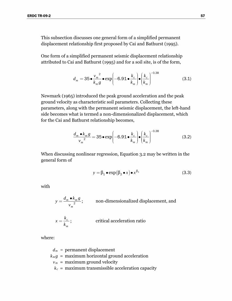
ERDC TR-09-2 57

This subsection discusses one general form of a simplified permanent displacement relationship first proposed by Cai and Bathurst (1995).

One form of a simplified permanent seismic displacement relationship attributed to Cai and Bathurst (1995) and for a soil site, is of the form,

.

exp .m cm

m m

v kd

k g k k

−⎛ ⎞ ⎛⎟ ⎟⎜ ⎜⎟ ⎟= • • − • •⎜ ⎜⎟ ⎟⎜ ⎜⎟ ⎟⎜ ⎜⎝ ⎠ ⎝

0 382

35 6 91 c

m

k ⎞

⎠ (3.1)

Newmark (1965) introduced the peak ground acceleration and the peak ground velocity as characteristic soil parameters. Collecting these parameters, along with the permanent seismic displacement, the left-hand side becomes what is termed a non-dimensionalized displacement, which for the Cai and Bathurst relationship becomes,

.

exp .m m c c

m mm

d k g k k

k kv

−⎛ ⎞ ⎛• ⎟ ⎟⎜ ⎜⎟ ⎟= • − • •⎜ ⎜⎟ ⎟⎜ ⎜⎟ ⎟⎜ ⎜⎝ ⎠ ⎝

0 38

2 35 6 91⎞

⎠ (3.2)

When discussing nonlinear regression, Equation 3.2 may be written in the general form of

( ) ββ exp βy x x= • • • 31 2 (3.3)

with

m m

m

d k gy

v

•= 2 ; non-dimensionalized displacement, and

c

m

kx

k= ; critical acceleration ratio

where:

dm = permanent displacement kmg = maximum horizontal ground acceleration vm = maximum ground velocity kc = maximum transmissible acceleration capacity

ERDC TR-09-2 58

for which β1, β2, and β3 are constants and the equation is nonlinear in β2.

The form of Equation 3.3 is now [x, y] as compared to the original form

,c m m

m m

k d k g

k v

⎡ ⎤•⎢⎢⎢ ⎥⎣ ⎦

2⎥⎥ of Equation 3.2.

Taking the natural log (ln) of both sides, Equation 3.3 becomes

( ) ( ) ( )ln ln β β β lny x= + • + •1 2 3 x (3.4)

which simplifies to

( ) ( )*ln β β β lny x x= + • + •1 2 3 (3.5)

with *β1 equal to ( )ln β1 , or ( )*β exp β=1 1 .

The transformation of Equation 3.3 to Equations 3.4 and 3.5 resulted in the altered form of the equation from (x, y) to (x, ln(y)) or specifically,

*( , )x y with , such that Equation 3.5 becomes, * ln( )y = y

* *β β β ln( )y x= + • + •1 2 3 x

)

(3.6)

From Equation 3.6, the set of basis functions (1, x, ln(x)) have a nonlinear

term, ln(x); however, the parameters ( *β , β , and β1 2 3 are constant and not

part of any nonlinear term.

Regression models which are a linear function of the parameters are called linear regression models. Therefore, a linear regression analysis can be applied to solve for these constant parameters.

The least squares fitting method is one of the simplest and most common applied forms of linear regression. This method will be used to estimate the parameters which will minimize the sum of squares of the y-distance from the specified, or produce the least possible value of S,

(* * *β β βN N

i i i ii i

S e y x x= =

)⎡ ⎤= = − + +⎢ ⎥⎣ ⎦∑ ∑2

21 2 3

1 1

(3.7)

ERDC TR-09-2 59

with

N = the total number of non-dimensionalized displacement terms = ln(x). *x

We can estimate the parameters by taking the partial derivatives of Equation 3.7 with respect to *β , β , and β1 2 3 , and setting the resultant equal

to zero.

( ) ( )

( ) ( )

( ) (

* * *

* * *

* * * *

β β ββ

β β ββ

β β ββ

N

i i ii

N

i i i ii

N

i i i ii

Sy x x

Sy x x x

Sy x x x

=

=

=

∂ ⎡ ⎤= − + + − =⎢ ⎥⎣ ⎦∂

∂ ⎡= − + + − =⎢⎣∂

∂ ⎡ ⎤= − + + − =⎢ ⎥⎣ ⎦∂

∑

∑

∑

1 2 311

1 2 312

1 2 313

2 1

2 0

2 0)

⎤⎥⎦

0

(3.8)

The estimates of *β , β , and β1 2 3

*

* *

*i i

are then represented by 3 linear equations

in 3 unknowns,

( )

( )

* *

*

* * * * *

β ( ) β β

β β β

β β β

N N N

i i ii i i

N N N N

i i i i i ii i i i

N N N N

i i i ii i i i

N x x y

x x x x x y

x x x x x y

= = =

= = = =

= = = =

+ + =

+ + =

+ + =

∑ ∑ ∑

∑ ∑ ∑ ∑

∑ ∑ ∑ ∑

1 2 31 1 1

21 2 3

1 1 1 1

2

1 2 31 1 1 1

(3.9)

The linear system of Equation 3.9 can be reduced to the equivalent system expressed in matrix form, M • β = Y, with matrix M, vector Y, and solving for vector β,

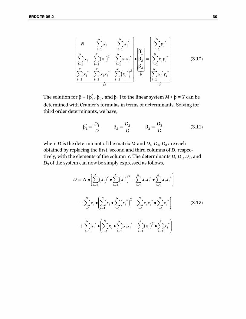
ERDC TR-09-2 60

( )

( )

* *

*

*

* * * *β

β

β

β

N N N

i ii i i

N N N N

i i i i i ii i i i

N N N N

i i i i ii i i i

M

N x x y

*

*

i

i

x x x x x y

x x x x x y

= = =

= = = =

= = = =

⎡ ⎤⎢ ⎥⎢ ⎥⎢ ⎥ ⎡ ⎤⎢ ⎥ ⎢ ⎥⎢ ⎥ ⎢ ⎥• =⎢ ⎥ ⎢ ⎥⎢ ⎥ ⎢ ⎥⎢ ⎥ ⎢ ⎥⎣ ⎦⎢ ⎥⎢ ⎥⎢ ⎥⎣ ⎦

∑ ∑ ∑

∑ ∑ ∑ ∑

∑ ∑ ∑ ∑

1 1 11

22

1 1 1 13

2

1 1 1 1

Y

⎥

⎡ ⎤⎢ ⎥⎢ ⎥⎢ ⎥⎢ ⎥⎢ ⎥⎢ ⎥⎢ ⎥⎢ ⎥⎢ ⎥⎢ ⎥⎢⎣ ⎦

(3.10)

The solution for β = [ *β , β , and β1 2 3 ] to the linear system M • β = Y can be

determined with Cramer’s formulas in terms of determinants. Solving for third order determinants, we have,

*βD

D= 1

1 βD

D= 2

2 βD

D= 3

3 (3.11)

where D is the determinant of the matrix M and D1, D2, D3 are each obtained by replacing the first, second and third columns of D, respec-tively, with the elements of the column Y. The determinants D, D1, D2, and D3 of the system can now be simply expressed as follows,

(3.12)

( ) ( )

( )

( )

* *

* *

* *

N N N N

i i i i ii i i i

N N N N N

i i i i i ii i i i i

N N N N N

i i i i ii i i i i

D N x x x x x x

x x x x x x

x x x x x x

= = = =

= = = = =

= = = = =

⎛ ⎞⎟⎜ ⎟= • • − •⎜ ⎟⎜ ⎟⎜⎝ ⎠

⎛ ⎞⎟⎜ ⎟− • • − •⎜ ⎟⎜ ⎟⎜⎝ ⎠

⎛ ⎞⎟⎜ ⎟+ • • − •⎜ ⎟⎜ ⎟⎜⎝ ⎠

∑ ∑ ∑ ∑

∑ ∑ ∑ ∑ ∑

∑ ∑ ∑ ∑ ∑

22

1 1 1 1

2

1 1 1 1 1

2

1 1 1 1 1

*

*

*

i

i

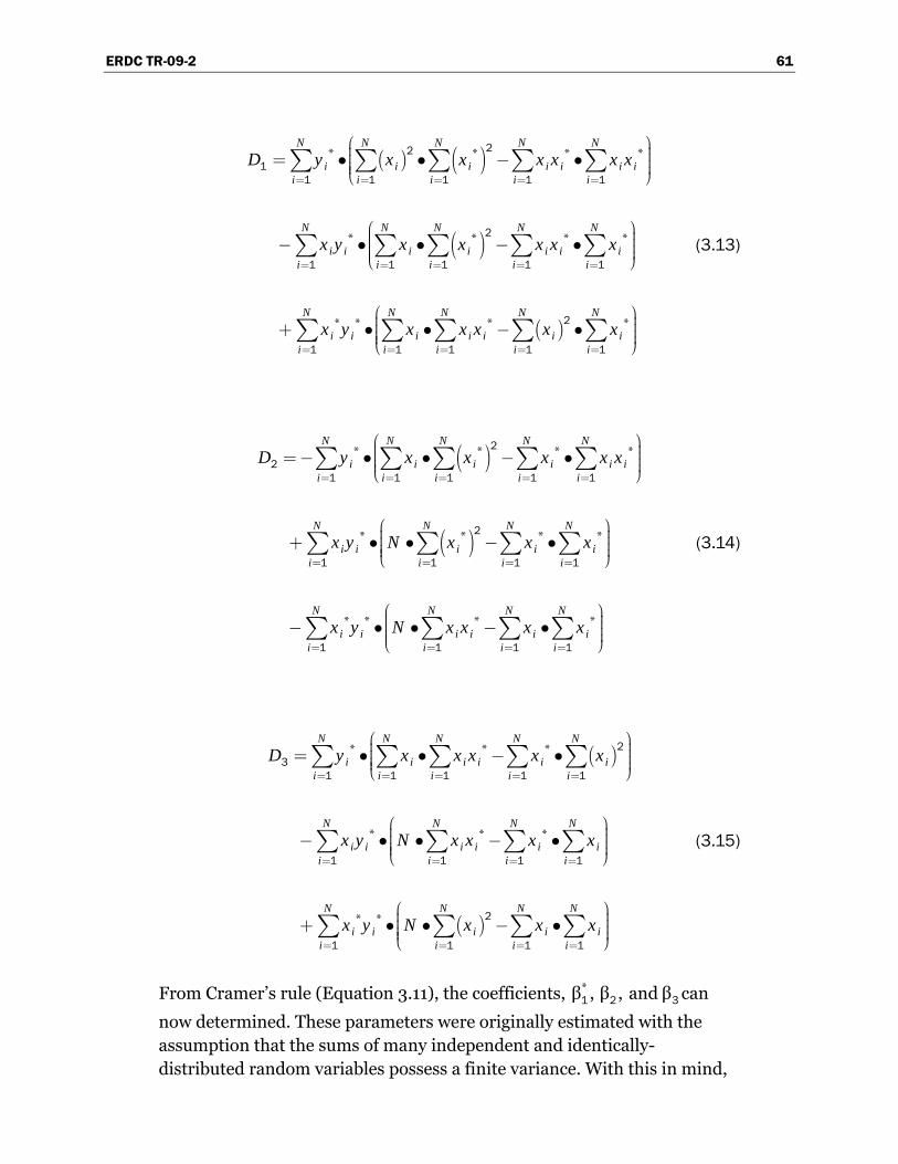
ERDC TR-09-2 61

(3.13)

( ) ( )

( )

( )

* * *

* * *

* * * *

N N N N N


N N N N N

i i i i i i ii i i i i

N N N N N

i i i i i i ii i i i i

D y x x x x x x

x y x x x x x

x y x x x x x

= = = = =

= = = = =

= = = = =

⎛ ⎞⎟⎜ ⎟= • • − •⎜ ⎟⎜ ⎟⎜⎝ ⎠

⎛ ⎞⎟⎜ ⎟− • • − •⎜ ⎟⎜ ⎟⎜⎝ ⎠

⎛ ⎞⎟⎜ ⎟+ • • − •⎜ ⎟⎜ ⎟⎜⎝ ⎠

∑ ∑ ∑ ∑ ∑

∑ ∑ ∑ ∑ ∑

∑ ∑ ∑ ∑ ∑

221

1 1 1 1 1

2

1 1 1 1 1

2

1 1 1 1 1

*

*

i

*ix

(3.14)

( )

( )

* * *

* * * *

* * * *

N N N N N

i i i i ii i i i i

N N N N

i i i i ii i i i

N N N N

i i i i i ii i i i

D y x x x x

x y N x x x

x y N x x x x

= = = = =

= = = =

= = = =

⎛ ⎞⎟⎜ ⎟=− • • − •⎜ ⎟⎜ ⎟⎜⎝ ⎠

⎛ ⎞⎟⎜ ⎟+ • • − •⎜ ⎟⎜ ⎟⎜⎝ ⎠

⎛ ⎞⎟⎜ ⎟− • • − •⎜ ⎟⎜ ⎟⎜⎝ ⎠

∑ ∑ ∑ ∑ ∑

∑ ∑ ∑ ∑

∑ ∑ ∑ ∑

2

21 1 1 1 1

2

1 1 1 1

1 1 1 1

(3.15)

( )

( )

* * *

* * *

* *

N N N N N


N N N N

i i i i i ii i i i

N N N N

i i i i ii i i i

D y x x x x x

x y N x x x x

x y N x x x

= = = = =

= = = =

= = = =

⎛ ⎞⎟⎜ ⎟= • • − •⎜ ⎟⎜ ⎟⎜⎝ ⎠

⎛ ⎞⎟⎜ ⎟− • • − •⎜ ⎟⎜ ⎟⎜⎝ ⎠

⎛ ⎞⎟⎜ ⎟+ • • − •⎜ ⎟⎜ ⎟⎜⎝ ⎠

∑ ∑ ∑ ∑ ∑

∑ ∑ ∑ ∑

∑ ∑ ∑ ∑

23

1 1 1 1 1

1 1 1 1

2

1 1 1 1

From Cramer’s rule (Equation 3.11), the coefficients, *β , β , and β1 2 3 can

now determined. These parameters were originally estimated with the assumption that the sums of many independent and identically-distributed random variables possess a finite variance. With this in mind,

ERDC TR-09-2 62

the residual error term or the variance, Equation 3.7, can be applied to determine the error in the estimates, the standard error (Std. error), defined as square root of the ratio of the square of the difference and the difference between N data points and the number of parameters (3),

Std. error = ( )* * *β β β

N

i ii

y x

N=

ix⎡ ⎤− + +⎢ ⎥⎣ ⎦−

∑2

1 2 31

3 3.16)

Typically, the smaller the Std. error, the more accurate the parameter estimation. As can be noted, the Std. error term will tend to get smaller with the increase in the number of data points. A 95 percent probability of non-exceedance will be used as an upper bound estimate. For a normally distributed variable, this value can be calculated by taking the product of the Std. error and 1.65, specifically from Equation 3.6 we can show that,

* *β β β ln( ) . .y x x Std er= + • + • + •1 2 3 1 65 ror (3.17)

Recalling that *β ln(β )=1 1 and ; taking the exponential of both

sides of Equation 3.6 and the residual error term, reintroduces a form of Equation 3.3, namely,

* ln( )y = y

( ) ββ exp β exp( . . )y x x Std error= • • • • •31 2 1 65 (3.18)

with ( )*β exp β=1 1 .

Finally, restoring to the original form of ,c m m

m m

k d k g

k v

⎡ ⎤•⎢ ⎥⎢ ⎥⎢ ⎥⎣ ⎦

2 gives us the non-

dimensionalized displacement equation for a 95 percent probability of non-exceedance,

( )β

β exp β exp . .m m c c

m mm

d k g k kStd error

k kv

⎛ ⎞ ⎛ ⎞• ⎟ ⎟⎜ ⎜⎟ ⎟= • • • • •⎜ ⎜⎟ ⎟⎜ ⎜⎟ ⎟⎜ ⎜⎝ ⎠ ⎝ ⎠

3

1 22 1 65 3.19)

and the non-dimensionalized displacement equation of the mean of the estimate as presented in row one of Table 3.1,

ERDC TR-09-2 63

β

β exp βm m c c

m mm

d k g k k

k kv

⎛ ⎞ ⎛• ⎟ ⎟⎜ ⎜⎟ ⎟= • • •⎜ ⎜⎟ ⎟⎜ ⎜⎟ ⎟⎜ ⎜⎝ ⎠ ⎝

3

1 22

⎞

⎠ (3.20)

The estimate and its Std. error can also be used to construct prediction intervals about the mean estimate. These prediction intervals reflect ranges that limit the average of the estimated value with a known proba-bility for a known distribution (a normal distribution for the transformed coordinate system in this case). For a selected N data set that is normally distributed, there is approximately a 68 percent probability that the average result will fall between one Std. error above the mean estimate and one Std. error below the mean estimate. The 68 percent prediction interval can be determined by modifying Equation 3.6 and adding/ subtracting the Std. error as follows,

* *β β β ln( ) .y x x Std error= + • + • ±1 2 3 (3.21)

or specifically,

* *β β β ln( ) .y x x Std error= + • + • +1 2 3 (3.21a)

and

* *β β β ln( ) .y x x Std er= + • + • −1 2 3 ror (3.21b)

Recalling that *β ln(β )=1 1 and * ln( )y y= ; taking the exponential of both

sides of Equations 3.21a and 3.21b reintroduces a form of Equation 3.3, namely,

( ) ββ exp β exp( . )y x x Std error= • • • •31 2 (3.22a)

and

( ) ββ exp β exp( . )y x x Std error= • • • • −31 2 (3.22b)


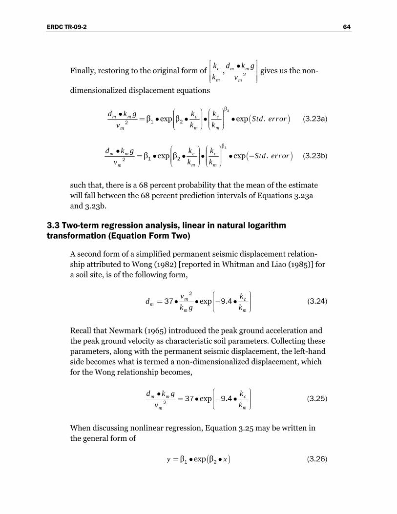
ERDC TR-09-2 64


m m

k d k g

k v

⎡ ⎤•⎢ ⎥⎢ ⎥⎢ ⎥⎣ ⎦

2 gives us the non-

dimensionalized displacement equations

(β

β exp β exp .m m c c

m mm

d k g k kStd error

k kv

⎛ ⎞ ⎛ ⎞• ⎟ ⎟⎜ ⎜⎟ ⎟= • • • •⎜ ⎜⎟ ⎟⎜ ⎜⎟ ⎟⎜ ⎜⎝ ⎠ ⎝ ⎠

3

1 22 ) (3.23a)

(β

β exp β exp .m m c c

m mm

d k g k kStd error

k kv

⎛ ⎞ ⎛ ⎞• ⎟ ⎟⎜ ⎜⎟ ⎟= • • • • −⎜ ⎜⎟ ⎟⎜ ⎜⎟ ⎟⎜ ⎜⎝ ⎠ ⎝ ⎠

3

1 22 ) (3.23b)

such that, there is a 68 percent probability that the mean of the estimate will fall between the 68 percent prediction intervals of Equations 3.23a and 3.23b.

3.3 Two-term regression analysis, linear in natural logarithm transformation (Equation Form Two)

A second form of a simplified permanent seismic displacement relation-ship attributed to Wong (1982) [reported in Whitman and Liao (1985)] for a soil site, is of the following form,

exp .m cm

m m

v kd

k g k

⎛ ⎞⎟⎜ ⎟= • • − •⎜ ⎟⎜ ⎟⎜⎝ ⎠

2

37 9 4 (3.24)

Recall that Newmark (1965) introduced the peak ground acceleration and the peak ground velocity as characteristic soil parameters. Collecting these parameters, along with the permanent seismic displacement, the left-hand side becomes what is termed a non-dimensionalized displacement, which for the Wong relationship becomes,

exp .m m c

mm

d k g k

kv

⎛ ⎞• ⎟⎜ ⎟= • − •⎜ ⎟⎜ ⎟⎜⎝ ⎠2 37 9 4 (3.25)

When discussing nonlinear regression, Equation 3.25 may be written in the general form of

( )β exp βy x= • •1 2 (3.26)

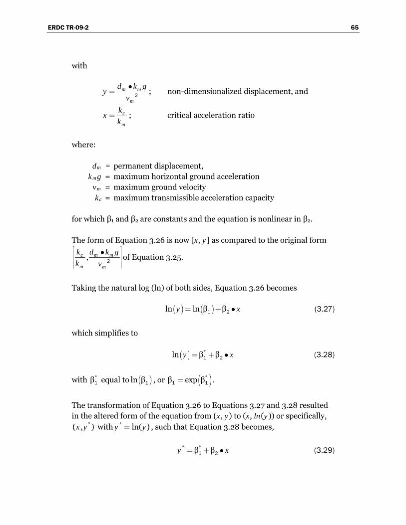
ERDC TR-09-2 65

with

m m

m

d k gy

v


c

m

kx


where:

dm = permanent displacement, kmg = maximum horizontal ground acceleration vm = maximum ground velocity kc = maximum transmissible acceleration capacity

for which β1 and β2 are constants and the equation is nonlinear in β2.


,c m m

m m

k d k g

k v

⎡ ⎤•⎢⎢⎢ ⎥⎣ ⎦


Taking the natural log (ln) of both sides, Equation 3.26 becomes

( ) ( )ln ln β βy x= +1 2 • (3.27)

which simplifies to

( ) *ln β βy x= + •1 2 (3.28)

with *β1 equal to ( )ln β1 , or ( )*β exp β=1 1 .

The transformation of Equation 3.26 to Equations 3.27 and 3.28 resulted in the altered form of the equation from (x, y) to (x, ln(y)) or specifically,

*( , )x y with , such that Equation 3.28 becomes, * ln( )y = y

* *β βy x= + •1 2 (3.29)

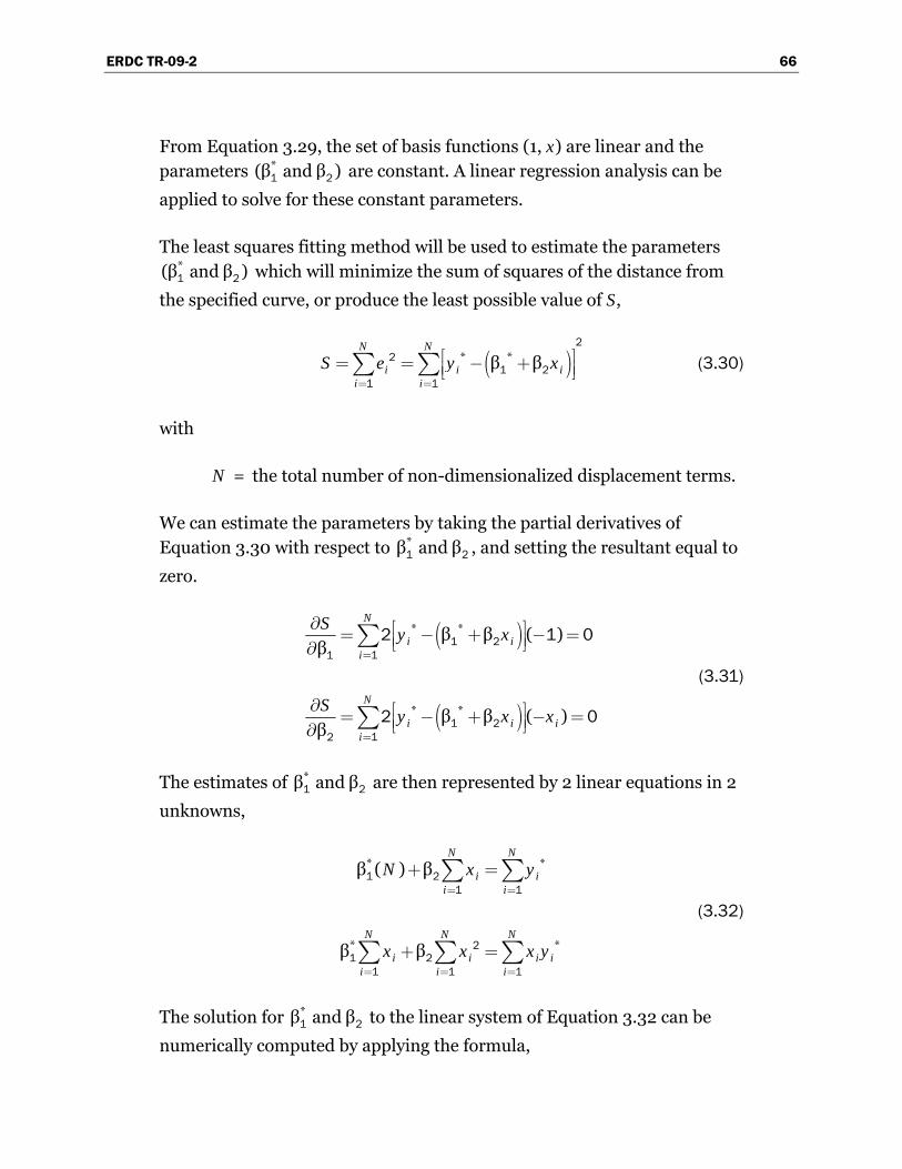
ERDC TR-09-2 66

From Equation 3.29, the set of basis functions (1, x) are linear and the parameters *(β and β )1 2 are constant. A linear regression analysis can be

applied to solve for these constant parameters.

The least squares fitting method will be used to estimate the parameters *(β and β )1 2

)i

which will minimize the sum of squares of the distance from

the specified curve, or produce the least possible value of S,

(* *β βN N

i ii i

S e y x= =

⎡ ⎤= = − +⎢ ⎥⎣ ⎦∑ ∑2

21 2

1 1

(3.30)

with

N = the total number of non-dimensionalized displacement terms.

We can estimate the parameters by taking the partial derivatives of Equation 3.30 with respect to *β and β1 2 , and setting the resultant equal to

zero.

( )

( )

* *

* *

β β ( )β

β β ( )β

N

i ii

N

i ii

Sy x

Sy x x

=

=

∂ ⎡ ⎤= − + − =⎢ ⎥⎣ ⎦∂

∂ ⎡ ⎤= − + − =⎢ ⎥⎣ ⎦∂

∑

∑

1 211

1 212

2 1

2 0i

0

(3.31)

The estimates of *β and β1 2

i i

are then represented by 2 linear equations in 2

unknowns,

* *

* *

β ( ) β

β β

N N

i ii i

N N N

i ii i i

N x y

x x x y

= =

= = =

+ =

+ =

∑ ∑

∑ ∑ ∑

1 21 1

21 2

1 1 1

(3.32)

The solution for *β and β1 2 to the linear system of Equation 3.32 can be

numerically computed by applying the formula,

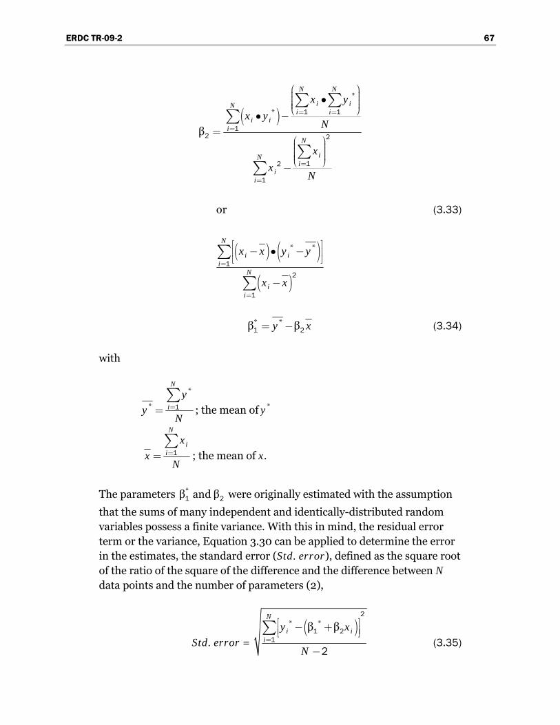
ERDC TR-09-2 67

( )

( ) ( )( )

*

*

* *

β

or

N N

i iNi i

i ii

N

iNi

ii

N

i ii

N

ii

x y

x yN

x

xN

x x y y

x x

= =

=

=

=

=

=

⎛ ⎞⎟⎜ ⎟•⎜ ⎟⎜ ⎟⎜⎝ ⎠• −=

⎛ ⎞⎟⎜ ⎟⎜ ⎟⎜ ⎟⎜⎝ ⎠−

⎡ ⎤− • −⎢ ⎥⎣ ⎦

−

∑ ∑∑

∑∑

∑

∑

1 1

12 2

12

1

12

1

(3.33)

* *β βy x= −1 2 (3.34)

with

*

*

N

i

y

yN==∑

1 ; the mean of *y

N

ii

x

xN==∑

1 ; the mean of x.

The parameters *β and β1 2 were originally estimated with the assumption

that the sums of many independent and identically-distributed random variables possess a finite variance. With this in mind, the residual error term or the variance, Equation 3.30 can be applied to determine the error in the estimates, the standard error (Std. error), defined as the square root of the ratio of the square of the difference and the difference between N data points and the number of parameters (2),

Std. error = ( )* *β β

N

i ii

y x

N=

⎡ ⎤− +⎢ ⎥⎣ ⎦−

∑2

1 21

2 (3.35)

ERDC TR-09-2 68

Typically, the smaller the Std. error, the more accurate the parameter esti-mation. As can be noted, the Std. error term will tend to get smaller with the increase in the number of data points. A 95 percent probability of non-exceedance will be used as an upper bound estimate. For a normally distributed variable, this value can be calculated by taking the product of the Std. error and 1.65, specifically from Equation 3.29 we can show that,

* *β β . .y x Std error= + • + •1 2 1 65 (3.36)

Recalling that ( )*β ln β=1 1 and ; taking the exponential of both

sides of Equation 3.29 and the residual error term, reintroduces a form of Equation 3.26, namely,

* ln( )y = y

) ( ) (β exp β exp . .y x Std e= • • • •1 2 1 65 rror (3.37)



m m

k d k g

k v

⎡ ⎤•⎢ ⎥⎢ ⎥⎢ ⎥⎣ ⎦

2 gives us the non-


(β exp β exp . .m m c

mm

d k g kStd error

kv

⎛ ⎞• ⎟⎜ ⎟= • • • •⎜ ⎟⎜ ⎟⎜⎝ ⎠1 22 1 65 ) (3.38)

and the non-dimensionalized displacement equation of the mean of the estimate, as presented in row two of Table 3.1,

β exp βm m c

mm

d k g k

kv

⎛ ⎞• ⎟⎜ ⎟= • •⎜ ⎟⎜ ⎟⎜⎝ ⎠1 22 (3.39)

The estimate and its Std. error can also be used to construct prediction intervals about the mean estimate. These prediction intervals reflect ranges that limit the average of the estimated value with a known proba-bility for a known distribution (a normal distribution for the transformed coordinate system in this case). For a selected N data set that is normally distributed, there is approximately a 68 percent probability that the average result will fall between one Std. error above the mean estimate

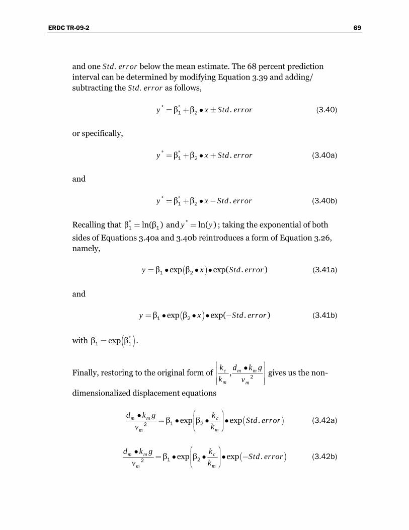
ERDC TR-09-2 69

and one Std. error below the mean estimate. The 68 percent prediction interval can be determined by modifying Equation 3.39 and adding/ subtracting the Std. error as follows,

* *β β .y x Std error= + • ±1 2 (3.40)

or specifically,

* *β β .y x Std error= + • +1 2 (3.40a)

and

* *β β .y x Std error= + • −1 2 (3.40b)

Recalling that *β ln(β )=1 1 and ; taking the exponential of both


* ln( )y = y

( )β exp β exp( . )y x Std error= • • •1 2 (3.41a)

and

( )β exp β exp( . )y x Std err= • • • −1 2 or (3.41b)



m m

k d k g

k v

⎡ ⎤•⎢ ⎥⎢ ⎥⎢ ⎥⎣ ⎦

2 gives us the non-


(β exp β exp .m m c

mm

d k g kStd error

kv

⎛ ⎞• ⎟⎜ ⎟= • • •⎜ ⎟⎜ ⎟⎜⎝ ⎠1 22 ) (3.42a)

(β exp β exp .m m c

mm

d k g kStd error

kv

⎛ ⎞• ⎟⎜ ⎟= • • • −⎜ ⎟⎜ ⎟⎜⎝ ⎠1 22 ) (3.42b)

ERDC TR-09-2 70


3.4 Two-term regression analysis, linear in common logarithm transformation (Equation Form One)

A third form of a simplified permanent seismic displacement relationship attributed to Richards and Elms (1979) for a soil site, is of the following form,

. m cm

m m

v kd

k g k

−⎛ ⎞⎟⎜ ⎟= • •⎜ ⎟⎜ ⎟⎜⎝ ⎠2

42

0 087 (3.43)

Recall that Newmark (1965) introduced the peak ground acceleration and the peak ground velocity as characteristic soil parameters. Collecting these parameters, along with the permanent seismic displacement, the left-hand side becomes what is termed a non-dimensionalized displacement, which for the Richards and Elms relationship becomes,

.m m c

mm

d k g k

kv

−⎛ ⎞• ⎟⎜ ⎟= •⎜ ⎟⎜ ⎟⎜⎝ ⎠

4

2 0 087 (3.44)

When discussing nonlinear regression, this Equation 3.44 may be written in the general form of

ββy x= • 54 (3.45)

with

m m

m

d k gy

v


c

m

kx


where:

dm = permanent displacement, kmg = maximum horizontal ground acceleration

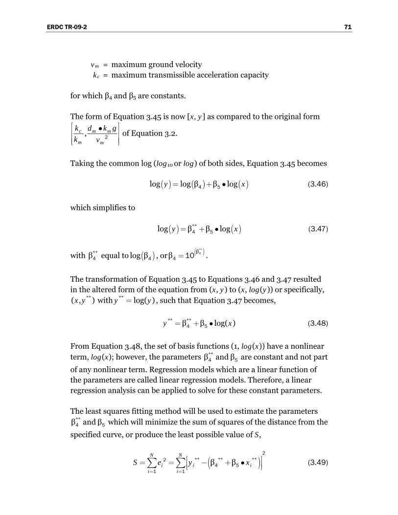
ERDC TR-09-2 71

vm = maximum ground velocity kc = maximum transmissible acceleration capacity

for which β4 and β5 are constants.


,c m m

m m

k d k g

k v

⎡ ⎤•⎢⎢⎢ ⎥⎣ ⎦


Taking the common log (log10 or log) of both sides, Equation 3.45 becomes

( ) ( ) ( )log log β β logy x= + •4 5 (3.46)

which simplifies to

( ) ( )**log β β logy x= + •4 5 (3.47)

with **β4 equal to ( )log β4 , or . ( )**ββ = 4

4 10

The transformation of Equation 3.45 to Equations 3.46 and 3.47 resulted in the altered form of the equation from (x, y) to (x, log(y)) or specifically,

**( , )x y with , such that Equation 3.47 becomes, ** log( )y = y

** **β β log( )y x= + •4 5 (3.48)

From Equation 3.48, the set of basis functions (1, log(x)) have a nonlinear term, log(x); however, the parameters **β and β4 5 are constant and not part

of any nonlinear term. Regression models which are a linear function of the parameters are called linear regression models. Therefore, a linear regression analysis can be applied to solve for these constant parameters.

The least squares fitting method will be used to estimate the parameters **β and β4 5

)

which will minimize the sum of squares of the distance from the

specified curve, or produce the least possible value of S,

(** ** **β βN N

i i ii i

S e y x= =

⎡ ⎤= = − + •⎢ ⎥⎣ ⎦∑ ∑2

24 5

1 1 (3.49)

ERDC TR-09-2 72

with

N = the total number of non-dimensionalized displacement terms. x** = log(x).

We can estimate the parameters by taking the partial derivatives of Equation 3.49 with respect to **β and β4 5 , and setting the resultant equal to

zero.

( )

( )

** ** ****

** ** ** **

β β ( )β

β β ( )β

N

i ii

N

i ii

Sy x

Sy x x

=

=

∂ ⎡ ⎤= − + • − =⎢ ⎥⎣ ⎦∂

∂ ⎡ ⎤= − + • − =⎢ ⎥⎣ ⎦∂

∑

∑

4 514

4 515

2 1

2 0i

0

(3.50)

The estimates of **β and β4 5

i

are then represented by 2 linear equations in 2

unknowns,

( )

** ** **

** ** ** ** **

β ( ) β

β β

N N

i ii i

N N N

i i ii i i

N x y

x x x y

= =

= = =

+ =

+ =

∑ ∑

∑ ∑ ∑

4 51 1

2

4 51 1 1

•

(3.51)

The solution for **β and β4 5 to the linear system of Equation 3.51 can be

numerically computed by applying the formulae,

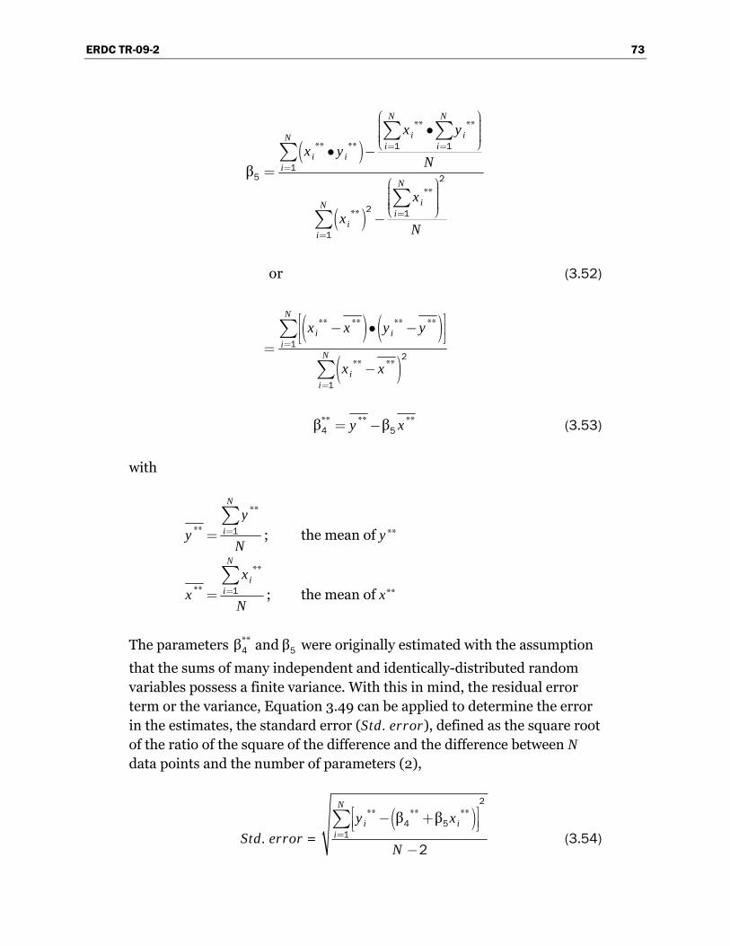
ERDC TR-09-2 73

( )

( )

( ) ( )( )

** **

** **

**

**

** ** ** **

** **

β

or

N N

i iNi i

i ii

N

iNi

ii

N

i ii

N

ii

x y

x yN

x

xN

x x y y

x x

= =

=

=

=

=

=

⎛ ⎞⎟⎜ ⎟•⎜ ⎟⎜ ⎟⎜⎝ ⎠• −=

⎛ ⎞⎟⎜ ⎟⎜ ⎟⎜ ⎟⎜⎝ ⎠−

⎡ ⎤− • −⎢ ⎥⎣ ⎦=−

∑ ∑∑

∑∑

∑

∑

1 1

15 2

2 1

1

12

1

(3.52)

** ** **β βy x= −4 5 (3.53)

with

**

**

N

i

y

yN==∑

1 ; the mean of y**

**

**

N

ii

x

xN

==∑

1 ; the mean of x**

The parameters **β and β4 5 were originally estimated with the assumption

that the sums of many independent and identically-distributed random variables possess a finite variance. With this in mind, the residual error term or the variance, Equation 3.49 can be applied to determine the error in the estimates, the standard error (Std. error), defined as the square root of the ratio of the square of the difference and the difference between N data points and the number of parameters (2),

Std. error = ( )** ** **β β

N

i ii

y x

N=

⎡ ⎤− +⎢ ⎥⎣ ⎦−

∑2

4 51

2 (3.54)

ERDC TR-09-2 74

Typically, the smaller the Std. error, the more accurate the parameter estimation. As can be noted, the Std. error term will tend to get smaller with the increase in the number of data points. A 95 percent probability of non-exceedance will be used as an upper bound estimate. For a normally distributed variable, this value can be calculated by taking the product of the Std. error and 1.65, specifically from Equation 3.48 we can show that,

** **β β log( ) . .y x Std error= + • + •4 5 1 65 (3.55)

Recalling that ( )**β log β=4 4 and ; taking the antilog of both

sides of Equation 3.55 with the residual error term, reintroduces a form of Equation 3.45, namely,

** log( )y = y

) (3.56) ( . .ββ Std errory x •= • •5 1 654 10

with . ( )**ββ = 4

4 10


m m

k d k g

k v

⎡ ⎤•⎢ ⎥⎢ ⎥⎢ ⎥⎣ ⎦

2 gives us the non-


(β

. .β Std errorm m c

mm

d k g k

kv•⎛ ⎞• ⎟⎜ ⎟= • •⎜ ⎟⎜ ⎟⎜⎝ ⎠

5

1 6542 10 ) (3.57)

and the non-dimensionalized displacement equation of the mean of the estimate, as presented in row three of Table 3.1,

β

βm m c

mm

d k g k

kv

⎛ ⎞• ⎟⎜ ⎟= •⎜ ⎟⎜ ⎟⎜⎝ ⎠

5

42 (3.58)

The estimate and its Std. error can also be used to construct prediction intervals about the mean estimate. These prediction intervals reflect ranges that limit the average of the estimated value with a known proba-bility for a known distribution (a normal distribution for the transformed coordinate system in this case). For a selected N data set that is normally distributed, there is approximately a 68 percent probability that the

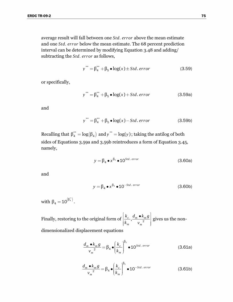
ERDC TR-09-2 75

average result will fall between one Std. error above the mean estimate and one Std. error below the mean estimate. The 68 percent prediction interval can be determined by modifying Equation 3.48 and adding/ subtracting the Std. error as follows,

** **β β log( ) .y x Std error= + • ±4 5 (3.59)

or specifically,

** **β β log( ) .y x Std error= + • +4 5 (3.59a)

and

** **β β log( ) .y x Std error= + • −4 5 (3.59b)

Recalling that ( )**β log β=4 4 and ** log( )y y= ; taking the antilog of both


(3.60a) β .β Std errory x= • •54 10

and

(3.60b) β .β Std errory x −= • •54 10

with . ( )**ββ = 4

4 10


m m

k d k g

k v

⎡ ⎤•⎢ ⎥⎢ ⎥⎢ ⎥⎣ ⎦

2 gives us the non-


β

.β Std errorm m c

mm

d k g k

kv

⎛ ⎞• ⎟⎜ ⎟= • •⎜ ⎟⎜ ⎟⎜⎝ ⎠

5

42 10 (3.61a)

β

.β Std errorm m c

mm

d k g k

kv−

⎛ ⎞• ⎟⎜ ⎟= • •⎜ ⎟⎜ ⎟⎜⎝ ⎠

5

42 10 (3.61b)

ERDC TR-09-2 76


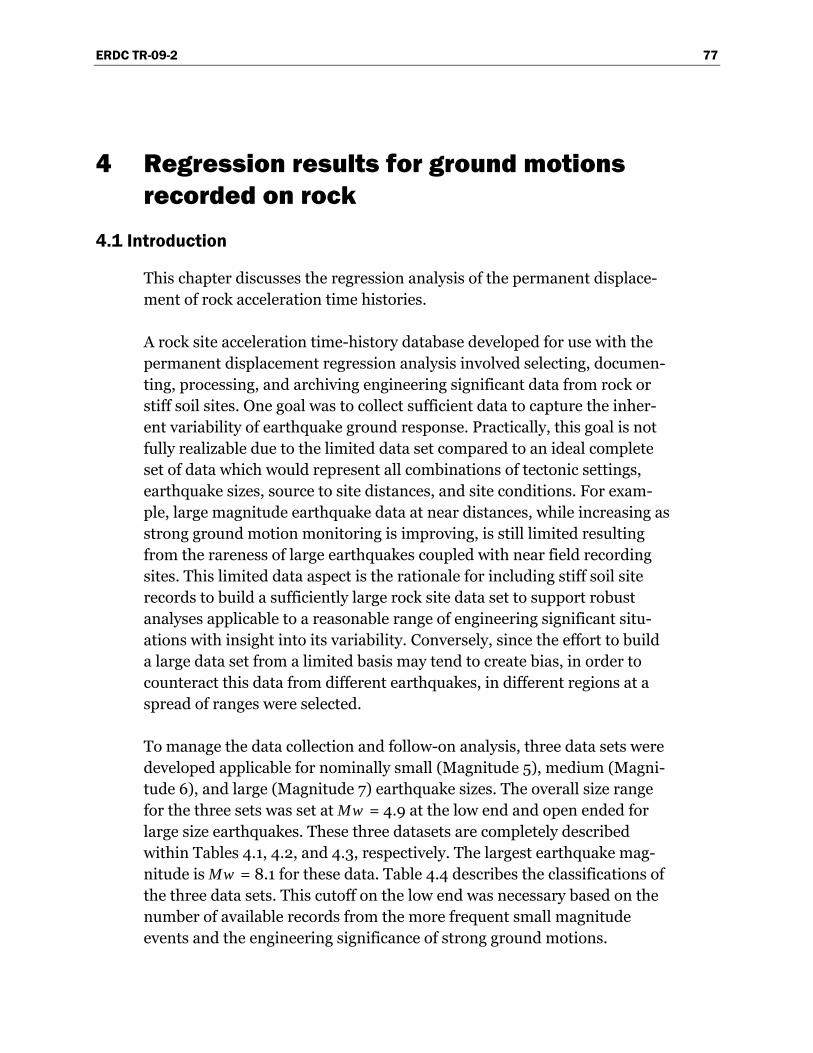
ERDC TR-09-2 77

4 Regression results for ground motions recorded on rock

4.1 Introduction

This chapter discusses the regression analysis of the permanent displace-ment of rock acceleration time histories.

A rock site acceleration time-history database developed for use with the permanent displacement regression analysis involved selecting, documen-ting, processing, and archiving engineering significant data from rock or stiff soil sites. One goal was to collect sufficient data to capture the inher-ent variability of earthquake ground response. Practically, this goal is not fully realizable due to the limited data set compared to an ideal complete set of data which would represent all combinations of tectonic settings, earthquake sizes, source to site distances, and site conditions. For exam-ple, large magnitude earthquake data at near distances, while increasing as strong ground motion monitoring is improving, is still limited resulting from the rareness of large earthquakes coupled with near field recording sites. This limited data aspect is the rationale for including stiff soil site records to build a sufficiently large rock site data set to support robust analyses applicable to a reasonable range of engineering significant situ-ations with insight into its variability. Conversely, since the effort to build a large data set from a limited basis may tend to create bias, in order to counteract this data from different earthquakes, in different regions at a spread of ranges were selected.

To manage the data collection and follow-on analysis, three data sets were developed applicable for nominally small (Magnitude 5), medium (Magni-tude 6), and large (Magnitude 7) earthquake sizes. The overall size range for the three sets was set at Mw = 4.9 at the low end and open ended for large size earthquakes. These three datasets are completely described within Tables 4.1, 4.2, and 4.3, respectively. The largest earthquake mag-nitude is Mw = 8.1 for these data. Table 4.4 describes the classifications of the three data sets. This cutoff on the low end was necessary based on the number of available records from the more frequent small magnitude events and the engineering significance of strong ground motions.

ERDC TR-09-2 78

In addition to a minimum magnitude restriction in the data search, an additional lower bound constraint was set at 0.007 g for the peak ground acceleration. The magnitude boundaries between the three earthquake data sets was arbitrary in the sense that there is not an implied physical basis for these separations at or near these magnitude boundaries of 4.9, 6.1, and 6.9, but were chosen based on populating a sufficient number in each set. In this respect, one should not expect to find different results in using data from either set near the dividing magnitudes.

Important to the documentation and use of these data are the definitions for the parameters of earthquake magnitude and site conditions. Inter-estingly, earthquake magnitude is not a simple data parameter because of the historical development of various earthquake magnitude scales and now backwards application of new magnitude scales to historical events. Earthquake magnitude scale to assess the size of an earthquake was ini-tially based on resulting levels of damage before seismic instrumentation was developed to measure ground motions. The initial use of the damage-based Mercali Intensity scale had evolved to determinations based on measured response of earthquake accelerographs and most recently to current use of a magnitude scale based on a mechanical concept based energy released, estimated on the area of the ruptured crust and the strength of crust. This current preferred scale in engineering seismology is the moment magnitude scale (Mw) and necessarily involves backwards assignment to historical data collected prior to its accepted and now rou-tine use. Table 4.5 is provided to illustrate this backward application and how the assigned earthquake magnitudes have changed for a few histori-cally significant earthquakes.

The Mw is a standard magnitude scale that is completely independent of the type of instrument such as Richter (M) and surface wave (Ms), which are indirect estimations of strain energy based on measured displacement amplitudes of seismic waves of certain periods and at certain distances from sources. The Mw is a more direct measure of energy since it is based on calculated frictional resistance over the area of fault slippage.

ERDC TR-09-2 79

Table 4.1. Master accelerograph table of magnitude 6.9 – 8.1.

M7 Master Accelerograph Table

PGA PGV PGD Ratio 1 Ratio 2

Lin Disp vm/km d*km/vm2

+ - + - + - + - + -

Set Rec# Filename Mw

Distance (hyp) km g% cm/s cm in./s/%g

AI 95%

Duration bracketed

Site Class Region Comp deg

Setting & Mech Earthquake Date Station

1 1 101_lpg1_090a.dat 7.0 33 0.442 -0.418 27.0 -33.8 8.50 -2.90 24.1 31.8 5.04 1.04 151 9.7 Rock(a) WUS H1 90 XX-RO-17 Loma Prieta 10/18/1989 Gilroy Array #1

2 102_lpg1_000a.dat 7.0 33 0.435 -0.375 32.5 -11.2 4.28 -9.49 29.4 11.8 1.73 27.71 95 13.2 Rock(a) WUS H2 0 XX-RO-17 Loma Prieta 10/18/1989 Gilroy Array #1

3 103_lpg1_0upa.dat 7.0 33 0.178 -0.210 8.3 -15.3 8.29 -3.79 18.4 28.6 20.99 3.36 26 4.3 Rock(a) WUS V UP XX-RO-17 Loma Prieta 10/18/1989 Gilroy Array #1

2 4 104_hmjt_360a.dat 7.1 52 0.168 -0.190 14.0 -23.2 5.40 -5.00 32.8 48.1 4.54 1.73 56 13.1 Rock(w/s) WUS H1 360 MF-SS-05 Hector Mine 10/16/1999 Joshua Tree Fire Sta

5 105_hmjt_090a.dat 7.1 52 0.102 -0.146 17.6 -17.1 7.00 -5.00 68.1 46.1 2.25 2.46 31 12.5 Rock(w/s) WUS H2 90 MF-SS-05 Hector Mine 10/16/1999 Joshua Tree Fire Sta

6 106_hmjt_0upa.dat 7.1 52 0.102 -0.121 9.0 -8.0 4.12 -4.16 34.7 25.9 5.10 7.77 27 14.0 Rock(w/s) WUS V UP MF-SS-05 Hector Mine 10/16/1999 Joshua Tree Fire Sta

3 7 107_lpld_000a.dat 7.1 26 0.388 -0.442 38.0 -84.3 12.03 -16.01 38.6 75.1 3.17 0.98 168 6.7 Rock WUS H1 0 XX-RO-17 Loma Prieta 10/18/1989 Lexington Dam -Abut

8 108_lpld_090a.dat 7.1 26 0.297 -0.409 31.9 -95.5 32.44 -10.98 42.3 91.9 9.27 0.48 158 7.1 Rock WUS H2 90 XX-RO-17 Loma Prieta 10/18/1989 Lexington Dam -Abut

9 109_lpld_0upa.dat 7.1 26 0.117 -0.133 25.9 -16.8 11.86 -16.77 87.1 49.8 2.03 7.74 18 5.2 Rock WUS V UP XX-RO-17 Loma Prieta 10/18/1989 Lexington Dam -Abut

4 10 110_inut_075a.dat 7.0 34 0.310 -0.224 15.8 -18.7 1.57 -2.32 20.1 32.8 1.90 1.46 87 8.3 Rock India H1 0 XX-XX-10 Uttarakshi, India 10/19/1991 IIT Roorkee, India

11 111_inut_345a.dat 7.0 34 0.227 -0.242 17.1 -9.6 1.82 -3.51 29.6 15.6 1.38 9.06 68 8.9 Rock India H2 345 XX-XX-10 Uttarakshi, India 10/19/1991 IIT Roorkee, India

12 112_inut_0upa.dat 7.0 34 0.189 -0.197 13.2 -7.6 2.93 -2.12 27.6 15.2 3.10 7.04 48 10.4 Rock India V V XX-XX-10 Uttarakshi, India 10/19/1991 IIT Roorkee, India

5 13 113_dz65_00xa.dat 7.1 23 0.496 -0.332 15.5 -16.5 1.58 -2.24 12.3 19.6 3.22 2.67 180 21.2 Rock Turkey H1 EW XX-SS-10 Duzce, Turkey 11/12/1999 LEDO Sta 6500

14 114_dz65_00ya.dat 7.1 23 0.619 -0.920 39.0 -27.1 2.76 -3.05 24.8 11.6 1.10 3.74 885 23.8 Rock Turkey H2 NS XX-SS-10 Duzce, Turkey 11/12/1999 LEDO Sta 6501

15 115_dz65_0upa.dat 7.1 23 0.182 -0.151 5.0 -5.3 1.32 -1.55 10.8 13.8 9.36 8.23 39 17.3 Rock Turkey V V XX-SS-10 Duzce, Turkey 11/12/1999 LEDO Sta 6502

6 16 116_kbku_000a.dat 6.9 31 0.290 -0.239 42.3 -54.8 8.92 -13.59 57.5 90.2 1.41 1.06 110 9.5 Rock Japan H1 0 XX-SS-18 Kobe, Japan 1/16/1995 Kobe University

17 117_kbku_090a.dat 6.9 31 0.310 -0.196 34.2 -20.2 7.17 -6.21 43.5 40.6 1.86 2.92 74 7.4 Rock Japan H2 90 XX-SS-18 Kobe, Japan 1/16/1995 Kobe University

18 118_kbku_0upa.dat 6.9 31 0.380 -0.324 16.5 -20.2 5.17 -6.55 17.1 24.5 7.06 5.12 59 6.8 Rock Japan V UP XX-SS-18 Kobe, Japan 1/16/1995 Kobe University

7 19 119_kbch_000a.dat 6.9 65 0.079 -0.093 5.9 -4.8 1.83 -2.90 29.4 20.3 4.08 11.51 11 6.2 Rock Japan H1 0 XX-SS-18 Kobe, Japan 1/20/1995 Chihaya

20 120_kbch_090a.dat 6.9 65 0.102 -0.108 3.4 -4.7 0.83 -1.08 13.0 17.1 7.25 5.19 14 8.5 Rock Japan H2 90 XX-SS-18 Kobe, Japan 1/20/1995 Chihaya

21 121_kbch_0upa.dat 6.9 65 0.067 -0.080 2.0 -2.4 1.14 -1.52 11.5 12.0 19.46 20.35 8 8.7 Rock Japan V UP XX-SS-18 Kobe, Japan 1/20/1995 Chihaya

8 22 122_lpuc_000a.dat 7.0 66 0.120 -0.157 17.2 -13.1 6.78 -5.20 56.6 33.1 2.68 4.62 26 9.8 Rock WUS H1 0 XX-RO-17 Loma Prieta 10/18/1989 Up. Crystal Spr Pulgas

23 123_lpuc_090a.dat 7.0 66 0.083 -0.086 10.3 -14.1 4.54 -5.85 48.9 64.3 3.46 2.49 16 7.8 Rock WUS H2 90 XX-RO-17 Loma Prieta 10/18/1989 Up. Crystal Spr Pulgas

24 124_lpuc_0upa.dat 7.0 66 0.041 -0.061 6.2 -4.3 2.51 -2.22 58.9 27.9 2.67 7.14 5 2.9 Rock WUS V UP XX-RO-17 Loma Prieta 10/18/1989 Up. Crystal Spr Pulgas

9 25 125_saak_090a.dat 7.1 79 0.208 -0.173 5.0 -4.6 0.70 -0.57 9.5 10.5 5.69 4.53 22 9.2 Rock Alaska H1 90 XX-XX-43 Southeast Alaska 5/2/1971 Adak AK Naval Base

26 126_saak_180a.dat 7.1 79 0.099 -0.117 3.2 -2.2 0.38 -0.57 13.0 7.5 3.48 13.10 6 3.7 Rock Alaska H2 180 XX-XX-43 Southeast Alaska 5/2/1971 Adak AK Naval Base

27 127_saak_0upa.dat 7.1 79 0.065 -0.063 2.0 -2.6 0.77 -0.51 12.4 16.3 11.75 4.61 4 1.1 Rock Alaska V UP XX-XX-43 Southeast Alaska 5/2/1971 Adak AK Naval Base

10 28 128_cmpt_090a.dat 7.0 16 1.040 -1.017 37.5 -42.4 12.59 -25.15 14.2 16.4 9.11 13.96 217 34.2 Rock WUS H2 90 XX-RV-10 Cape Mendocino 4/25/1992 Cape Mendocino - Petrolia

29 129_cmpt_000a.dat 7.0 16 1.498 -0.494 38.2 -129.2 11.80 -54.21 10.0 103.0 11.89 1.57 543 37.9 Rock WUS H1 180 XX-RV-10 Cape Mendocino 4/25/1992 Cape Mendocino - Petrolia

30 130_cmpt_0upa.dat 7.0 16 0.514 -0.755 70.0 -54.7 133.42 -13.94 53.6 28.5 13.73 3.45 125 7.9 Rock WUS V UP XX-RV-10 Cape Mendocino 4/25/1992 Cape Mendocino - Petrolia

11 31 131_lnbb_360a.dat 7.3 46 0.170 -0.192 14.0 -10.9 7.86 -9.44 32.3 22.4 6.71 14.89 56.64 25.1 Rock WUS H1 360 XX-SS-05 Landers 6/28/1992 Big Bear Lake - Civic Center

32 132_lnbb_270a.dat 7.3 46 0.165 -0.116 7.2 -7.6 3.43 -3.31 17.3 25.8 10.55 6.52 50.35 21.6 Rock WUS H2 270 XX-SS-05 Landers 6/28/1992 Big Bear Lake - Civic Center

33 133_lnbb_0upa.dat 7.3 46 0.064 -0.081 4.0 -4.1 1.18 -1.54 24.3 20.2 4.72 7.10 13.29 15.6 Rock WUS V UP XX-SS-05 Landers 6/28/1992 Big Bear Lake - Civic Center

12 34 134_tbir_190a.dat 7.4 18 0.401 -0.277 16.5 -25.0 9.86 -8.78 16.2 35.5 14.30 3.83 152.85 36.9 Rock Iran H1 190 XX-XX-XX Tabas, Iran 9/16/1978 Ministry of Housing & Urban Dev.

35 135_tbir_080a.dat 7.4 18 0.371 -0.290 24.5 -24.4 22.29 -23.32 25.9 33.1 13.58 11.15 160.34 36.8 Rock Iran H2 80 XX-XX-XX Tabas, Iran 9/16/1978 Ministry of Housing & Urban Dev.

36 136_tbir_0upa.dat 7.4 18 0.180 -0.189 12.1 -10.7 10.22 -6.28 26.4 22.3 12.38 10.17 84.9 35.7 Rock Iran V UP XX-XX-XX Tabas, Iran 9/16/1978 Ministry of Housing & Urban Dev.

ERDC TR-09-2 80



Lin Disp vm/km d*km/vm2

+ - + - + - + - + -



AI 95%

Duration bracketed


Setting & Mech Earthquake Date Station

13 37 137_elob_180a.dat 7.6 109 0.428 -0.404 35.7 -38.4 8.68 -4.12 32.8 37.4 2.86 1.11 346.19 33.7 Rock El Salvador H1 180 XX-XX-60 El Salvador 1/13/2001 Observatorio

38 138_elob_090a.dat 7.6 109 0.349 -0.379 24.6 -26.1 4.63 -5.82 27.7 27.1 2.62 3.17 225.96 31.0 Rock El Salvador H2 90 XX-XX-60 El Salvador 1/13/2001 Observatorio

39 139_elob_0upa.dat 7.6 109 0.253 -0.306 13.0 -11.6 6.33 -5.38 20.2 14.9 9.28 12.07 156.2 33.9 Rock El Salvador V UP XX-XX-60 El Salvador 1/13/2001 Observatorio

14 40 140_elsm_360a.dat 7.6 80 0.581 -0.881 26.6 -27.8 4.06 -5.95 18.0 12.4 3.26 6.65 866.49 33.3 Rock El Salvador H1 360 XX-XX-60 El Salvador 1/13/2001 Santiago de Maria

41 141_elsm_090a.dat 7.6 80 0.646 -0.716 40.4 -40.1 8.41 -6.70 24.6 22.0 3.27 2.93 1057.8 35.2 Rock El Salvador H2 90 XX-XX-60 El Salvador 1/13/2001 Santiago de Maria

42 142_elsm_0upa.dat 7.6 80 0.440 -0.402 14.0 -16.1 6.88 -4.66 12.5 15.7 15.18 7.10 302 31.1 Rock El Salvador V UP XX-XX-60 El Salvador 1/13/2001 Santiago de Maria

15 43 143_itst_000a.dat 6.9 32 0.251 -0.231 36.4 -27.7 10.61 -11.37 57.2 47.2 1.97 3.36 107.28 17.3 Rock Iprina, Italy H1 0 XX-XX-9.5 Iprina, Italy 11/23/1980 ENEL, Struno, Italy

44 144_itst_270a.dat 6.9 32 0.287 -0.358 49.2 -51.8 17.54 -32.36 67.5 57.0 2.04 4.23 127.08 23.7 Rock Iprina, Italy H2 270 XX-XX-9.5 Iprina, Italy 11/23/1980 ENEL, Struno, Italy

45 145_itst_0upa.dat 6.9 32 0.260 -0.166 16.7 -25.6 10.29 -6.36 25.3 60.8 9.41 1.58 46.52 11.6 Rock Iprina, Italy V UP XX-XX-9.5 Iprina, Italy 11/23/1980 ENEL, Struno, Italy

16 46 146_itba_000a.dat 6.9 25 0.133 -0.139 22.1 -15.8 7.96 -9.24 65.2 44.6 2.14 5.07 30.35 9.1 Rock Iprina, Italy H1 0 XX-XX-9.5 Iprina, Italy 11/23/1980 ENEL, Bagnoli, Italy

47 147_itba_270a.dat 6.9 25 0.202 -0.177 31.9 -17.8 9.59 -9.24 62.1 39.5 1.87 5.07 38.97 10.6 Rock Iprina, Italy H2 270 XX-XX-9.5 Iprina, Italy 11/23/1980 ENEL, Bagnoli, Italy

48 148_itba_0upa.dat 6.9 25 0.108 -0.090 11.8 -14.1 4.80 -5.75 43.0 61.9 3.65 2.54 15.66 7.2 Rock Iprina, Italy V UP XX-XX-9.5 Iprina, Italy 11/23/1980 ENEL, Bagnoli, Italy

17 49 149_itbi_000a.dat 6.9 25 0.061 -0.100 23.4 -14.4 14.03 -12.65 152.2 56.7 1.52 5.96 16.91 9.9 Rock Iprina, Italy H1 0 XX-XX-9.5 Iprina, Italy 11/23/1980 ENEL, Bisaccia, Italy

50 150_itbi_270a.dat 6.9 25 0.083 -0.057 11.9 -12.5 2.89 -2.93 56.6 86.9 1.65 1.04 12.46 2.1 Rock Iprina, Italy H2 270 XX-XX-9.5 Iprina, Italy 11/23/1980 ENEL, Bisaccia, Italy

51 151_itbi_0upa.dat 6.9 25 0.055 -0.067 14.1 -11.6 11.12 -9.09 100.9 68.1 3.02 4.46 10.49 0.8 Rock Iprina, Italy V UP XX-XX-9.5 Iprina, Italy 11/23/1980 ENEL, Bisaccia, Italy

18 52 152_tasm_0ewa.dat 7.3 73 0.112 -0.136 13.5 -9.5 5.90 -4.77 47.3 27.4 3.57 7.11 28.95 9.1 Rock Taiwan H1 EW XX-XX-15 Smart, Taiwan 11/14/1986 Smart, Taiwan

53 153_tasm_0nsa.dat 7.3 73 0.139 -0.143 12.4 -10.5 3.43 -6.06 35.2 29.0 3.02 7.67 33.87 37.6 Rock Taiwan H2 NS XX-XX-15 Smart, Taiwan 11/14/1986 Smart, Taiwan

54 154_tasm_0dna.dat 7.3 73 0.042 -0.052 4.8 -5.4 1.96 -3.05 45.3 40.8 3.49 5.33 6.44 0.0 Rock Taiwan V DN XX-XX-15 Smart, Taiwan 11/14/1986 Smart, Taiwan

19 55 155_tach_45ea.dat 7.6 78 0.401 -0.474 36.6 -32.7 21.51 -50.39 35.9 27.1 6.32 21.95 125.55 21.7 Rock Taiwan H1 E XX-XX-6.8 ChiChi 9/20/1999 ChiChi, Taiwan

56 156_tach_45na.dat 7.6 78 0.512 -0.250 27.8 -39.1 13.59 -14.20 21.4 61.5 8.81 2.28 105.88 14.2 Rock Taiwan H2 N XX-XX-6.8 ChiChi 9/20/1999 ChiChi, Taiwan

57 157_tach_45va.dat 7.6 78 0.181 -0.361 21.4 -15.9 12.43 -22.90 46.6 17.3 4.81 32.27 33.95 12.6 Rock Taiwan V V XX-XX-6.8 ChiChi 9/20/1999 ChiChi, Taiwan

20 58 158_tach_71ea.dat 7.6 17 0.567 -0.524 37.6 -44.5 13.76 -12.62 26.1 33.4 5.40 3.28 839.55 58.2 Rock Taiwan H1 E XX-XX-6.8 ChiChi 9/20/1999 ChiChi, Taiwan

59 159_tach_71na.dat 7.6 17 0.567 -0.655 47.0 -69.4 48.34 -49.53 32.6 41.7 12.17 6.60 855.32 58.7 Rock Taiwan H2 N XX-XX-6.8 ChiChi 9/20/1999 ChiChi, Taiwan

60 160_tach_71va.dat 7.6 17 0.449 -0.348 31.3 -34.8 23.33 -31.34 27.4 39.4 10.50 8.83 248.74 30.0 Rock Taiwan V V XX-XX-6.8 ChiChi 9/20/1999 ChiChi, Taiwan

21 61 261_mhlu_000a.dat 8.1 84 0.164 -0.169 21.6 -21.0 22.52 -14.68 51.8 48.9 7.78 5.53 91.67 31.8 Rock Mexico H1 N00W Su-IT-27 Michoacan 9/19/1985 La Union, Mexico

62 262_mhli_090a.dat 8.1 84 0.151 -0.141 10.3 -13.2 8.59 -5.23 27.0 36.8 11.88 4.16 81.12 31.8 Rock Mexico H2 N90W Su-IT-27 Michoacan 9/19/1985 La Union, Mexico

63 263_mhlu_0upa.dat 8.1 84 0.107 -0.132 14.4 -15.0 13.15 -16.03 52.8 44.8 6.69 9.20 36.94 23.7 Rock Mexico V V Su-IT-27 Michoacan 9/19/1985 La Union, Mexico

22 64 264_pich_000a.dat 7.8 84 0.259 -0.205 9.6 -11.7 3.72 -2.76 14.6 22.5 10.31 4.06 140.48 23.2 Rock Chile H1 0 Su-IT-33 Valparaiso 3/3/1985 Pichemu, Chile

65 265_pich_090a.dat 7.8 84 0.151 -0.178 12.4 -12.4 3.63 -3.92 32.5 27.5 3.47 4.43 76.65 22.5 Rock Chile H2 90 Su-IT-33 Valparaiso 3/3/1985 Pichemu, Chile

66 266_pich_0upa.dat 7.8 84 0.107 -0.121 5.1 -5.9 1.95 -1.77 18.8 19.3 7.81 5.95 24.04 18.2 Rock Chile V UP Su-IT-33 Valparaiso 3/3/1985 Pichemu, Chile

23 67 267_pach_140a.dat 7.8 84 0.231 -0.230 12.4 -11.3 1.67 -1.88 21.1 19.4 2.47 3.31 254.62 59.1 Rock Chile H 140 Su-IT-33 Valparaiso 3/3/1985 Papudo Chile

68 268_pach_0upa.dat 7.8 84 0.197 -0.177 6.2 -5.2 1.17 -1.12 12.5 11.6 5.79 7.22 93.93 50.3 Rock Chile V UP Su-IT-33 Valparaiso 3/3/1985 Papudo Chile

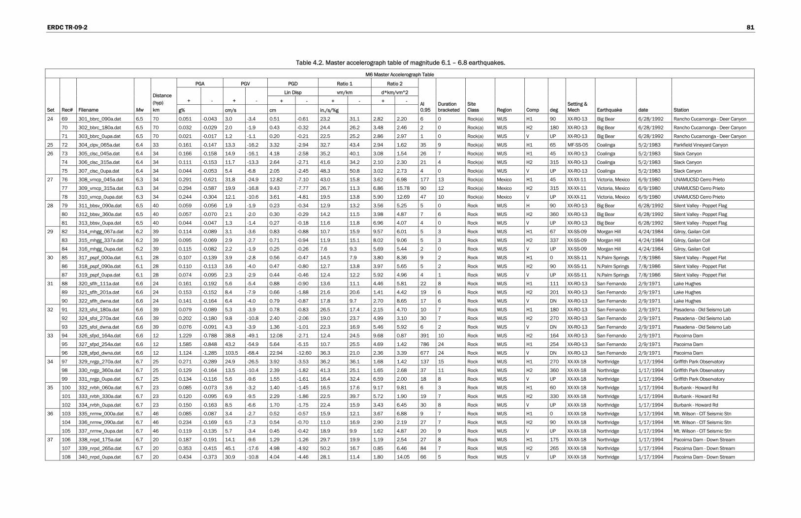
ERDC TR-09-2 81

Table 4.2. Master accelerograph table of magnitude 6.1 – 6.8 earthquakes.



Lin Disp vm/km d*km/vm^2 + - + - + - + - + -



AI 0.95

Duration bracketed


Setting & Mech Earthquake date Station

24 69 301_bbrc_090a.dat 6.5 70 0.051 -0.043 3.0 -3.4 0.51 -0.61 23.2 31.1 2.82 2.20 6 0 Rock(a) WUS H1 90 XX-RO-13 Big Bear 6/28/1992 Rancho Cucamonga - Deer Canyon

70 302_bbrc_180a.dat 6.5 70 0.032 -0.029 2.0 -1.9 0.43 -0.32 24.4 26.2 3.48 2.46 2 0 Rock(a) WUS H2 180 XX-RO-13 Big Bear 6/28/1992 Rancho Cucamonga - Deer Canyon

71 303_bbrc_0upa.dat 6.5 70 0.021 -0.017 1.2 -1.1 0.20 -0.21 22.5 25.2 2.86 2.97 1 0 Rock(a) WUS V UP XX-RO-13 Big Bear 6/28/1992 Rancho Cucamonga - Deer Canyon

25 72 304_clpv_065a.dat 6.4 33 0.161 -0.147 13.3 -16.2 3.32 -2.94 32.7 43.4 2.94 1.62 35 9 Rock(a) WUS H1 65 MF-SS-05 Coalinga 5/2/1983 Parkfield Vineyard Canyon

26 73 305_clsc_045a.dat 6.4 34 0.166 -0.158 14.9 -16.1 4.18 -2.58 35.2 40.1 3.08 1.54 26 7 Rock(a) WUS H1 45 XX-RO-13 Coalinga 5/2/1983 Slack Canyon

74 306_clsc_315a.dat 6.4 34 0.111 -0.153 11.7 -13.3 2.64 -2.71 41.6 34.2 2.10 2.30 21 4 Rock(a) WUS H2 315 XX-RO-13 Coalinga 5/2/1983 Slack Canyon

75 307_clsc_0upa.dat 6.4 34 0.044 -0.053 5.4 -6.8 2.05 -2.45 48.3 50.8 3.02 2.73 4 0 Rock(a) WUS V UP XX-RO-13 Coalinga 5/2/1983 Slack Canyon

27 76 308_vmcp_045a.dat 6.3 34 0.291 -0.621 31.8 -24.9 12.82 -7.10 43.0 15.8 3.62 6.98 177 13 Rock(a) Mexico H1 45 XX-XX-11 Victoria, Mexico 6/9/1980 UNAMUCSD Cerro Prieto

77 309_vmcp_315a.dat 6.3 34 0.294 -0.587 19.9 -16.8 9.43 -7.77 26.7 11.3 6.86 15.78 90 12 Rock(a) Mexico H2 315 XX-XX-11 Victoria, Mexico 6/9/1980 UNAMUCSD Cerro Prieto

78 310_vmcp_0upa.dat 6.3 34 0.244 -0.304 12.1 -10.6 3.61 -4.81 19.5 13.8 5.90 12.69 47 10 Rock(a) Mexico V UP XX-XX-11 Victoria, Mexico 6/9/1980 UNAMUCSD Cerro Prieto

28 79 311_bbsv_090a.dat 6.5 40 0.059 -0.056 1.9 -1.9 0.23 -0.34 12.9 13.2 3.56 5.25 5 0 Rock WUS H 90 XX-RO-13 Big Bear 6/28/1992 Silent Valley - Poppet Flag

80 312_bbsv_360a.dat 6.5 40 0.057 -0.070 2.1 -2.0 0.30 -0.29 14.2 11.5 3.98 4.87 7 6 Rock WUS H2 360 XX-RO-13 Big Bear 6/28/1992 Silent Valley - Poppet Flag

81 313_bbsv_0upa.dat 6.5 40 0.044 -0.047 1.3 -1.4 0.27 -0.18 11.6 11.8 6.96 4.07 4 0 Rock WUS V UP XX-RO-13 Big Bear 6/28/1992 Silent Valley - Poppet Flag

29 82 314_mhgg_067a.dat 6.2 39 0.114 -0.089 3.1 -3.6 0.83 -0.88 10.7 15.9 9.57 6.01 5 3 Rock WUS H1 67 XX-SS-09 Morgan Hill 4/24/1984 Gilroy, Gailan Coll

83 315_mhgg_337a.dat 6.2 39 0.095 -0.069 2.9 -2.7 0.71 -0.94 11.9 15.1 8.02 9.06 5 3 Rock WUS H2 337 XX-SS-09 Morgan Hill 4/24/1984 Gilroy, Gailan Coll

84 316_mhgg_0upa.dat 6.2 39 0.115 -0.082 2.2 -1.9 0.25 -0.26 7.6 9.3 5.69 5.44 2 0 Rock WUS V UP XX-SS-09 Morgan Hill 4/24/1984 Gilroy, Gailan Coll

30 85 317_pspf_000a.dat 6.1 28 0.107 -0.139 3.9 -2.8 0.56 -0.47 14.5 7.9 3.80 8.36 9 2 Rock WUS H1 0 XX-SS-11 N.Palm Springs 7/8/1986 Silent Valley - Poppet Flat

86 318_pspf_090a.dat 6.1 28 0.110 -0.113 3.6 -4.0 0.47 -0.80 12.7 13.8 3.97 5.65 5 2 Rock WUS H2 90 XX-SS-11 N.Palm Springs 7/8/1986 Silent Valley - Poppet Flat

87 319_pspf_0upa.dat 6.1 28 0.074 -0.095 2.3 -2.9 0.44 -0.46 12.4 12.2 5.92 4.96 4 1 Rock WUS V UP XX-SS-11 N.Palm Springs 7/8/1986 Silent Valley - Poppet Flat

31 88 320_sflh_111a.dat 6.6 24 0.161 -0.192 5.6 -5.4 0.88 -0.90 13.6 11.1 4.46 5.81 22 8 Rock WUS H1 111 XX-RO-13 San Fernando 2/9/1971 Lake Hughes

89 321_sflh_201a.dat 6.6 24 0.153 -0.152 8.4 -7.9 0.66 -1.88 21.6 20.6 1.41 4.42 19 6 Rock WUS H2 201 XX-RO-13 San Fernando 2/9/1971 Lake Hughes

90 322_sflh_dwna.dat 6.6 24 0.141 -0.164 6.4 -4.0 0.79 -0.87 17.8 9.7 2.70 8.65 17 6 Rock WUS V DN XX-RO-13 San Fernando 2/9/1971 Lake Hughes

32 91 323_sfol_180a.dat 6.6 39 0.079 -0.089 5.3 -3.9 0.78 -0.83 26.5 17.4 2.15 4.70 10 7 Rock WUS H1 180 XX-RO-13 San Fernando 2/9/1971 Pasadena - Old Seismo Lab

92 324_sfol_270a.dat 6.6 39 0.202 -0.180 9.8 -10.8 2.40 -2.06 19.0 23.7 4.99 3.10 30 7 Rock WUS H2 270 XX-RO-13 San Fernando 2/9/1971 Pasadena - Old Seismo Lab

93 325_sfol_dwna.dat 6.6 39 0.076 -0.091 4.3 -3.9 1.36 -1.01 22.3 16.9 5.46 5.92 6 2 Rock WUS V DN XX-RO-13 San Fernando 2/9/1971 Pasadena - Old Seismo Lab

33 94 326_sfpd_164a.dat 6.6 12 1.229 -0.788 38.8 -49.1 12.08 -2.71 12.4 24.5 9.68 0.87 391 10 Rock WUS H2 164 XX-RO-13 San Fernando 2/9/1971 Pacoima Dam

95 327_sfpd_254a.dat 6.6 12 1.585 -0.848 43.2 -54.9 5.64 -5.15 10.7 25.5 4.69 1.42 786 24 Rock WUS H1 254 XX-RO-13 San Fernando 2/9/1971 Pacoima Dam

96 328_sfpd_dwna.dat 6.6 12 1.124 -1.285 103.5 -68.4 22.94 -12.60 36.3 21.0 2.36 3.39 677 24 Rock WUS V DN XX-RO-13 San Fernando 2/9/1971 Pacoima Dam

34 97 329_nrgp_270a.dat 6.7 25 0.271 -0.289 24.9 -26.5 3.92 -3.53 36.2 36.1 1.68 1.42 137 15 Rock WUS H1 270 XX-XX-18 Northridge 1/17/1994 Griffith Park Observatory

98 330_nrgp_360a.dat 6.7 25 0.129 -0.164 13.5 -10.4 2.39 -1.82 41.3 25.1 1.65 2.68 37 11 Rock WUS H2 360 XX-XX-18 Northridge 1/17/1994 Griffith Park Observatory

99 331_nrgp_0upa.dat 6.7 25 0.134 -0.116 5.6 -9.6 1.55 -1.61 16.4 32.4 6.59 2.00 18 8 Rock WUS V UP XX-XX-18 Northridge 1/17/1994 Griffith Park Observatory

35 100 332_nrbh_060a.dat 6.7 23 0.085 -0.073 3.6 -3.2 1.40 -1.45 16.5 17.6 9.17 9.81 6 3 Rock WUS H1 60 XX-XX-18 Northridge 1/17/1994 Burbank - Howard Rd

101 333_nrbh_330a.dat 6.7 23 0.120 -0.095 6.9 -9.5 2.29 -1.86 22.5 39.7 5.72 1.90 19 7 Rock WUS H2 330 XX-XX-18 Northridge 1/17/1994 Burbank - Howard Rd

102 334_nrbh_0upa.dat 6.7 23 0.150 -0.163 8.5 -6.6 1.70 -1.75 22.4 15.9 3.43 6.45 30 8 Rock WUS V UP XX-XX-18 Northridge 1/17/1994 Burbank - Howard Rd

36 103 335_nrmw_000a.dat 6.7 46 0.085 -0.087 3.4 -2.7 0.52 -0.57 15.9 12.1 3.67 6.88 9 7 Rock WUS H1 0 XX-XX-18 Northridge 1/17/1994 Mt. Wilson - CIT Seismic Stn

104 336_nrmw_090a.dat 6.7 46 0.234 -0.169 6.5 -7.3 0.54 -0.70 11.0 16.9 2.90 2.19 27 7 Rock WUS H2 90 XX-XX-18 Northridge 1/17/1994 Mt. Wilson - CIT Seismic Stn

105 337_nrmw_0upa.dat 6.7 46 0.119 -0.135 5.7 -3.4 0.45 -0.42 18.9 9.9 1.62 4.87 20 9 Rock WUS V UP XX-XX-18 Northridge 1/17/1994 Mt. Wilson - CIT Seismic Stn

37 106 338_nrpd_175a.dat 6.7 20 0.187 -0.191 14.1 -9.6 1.29 -1.26 29.7 19.9 1.19 2.54 27 8 Rock WUS H1 175 XX-XX-18 Northridge 1/17/1994 Pacoima Dam - Down Stream

107 339_nrpd_265a.dat 6.7 20 0.353 -0.415 45.1 -17.6 4.98 -4.92 50.2 16.7 0.85 6.46 84 7 Rock WUS H2 265 XX-XX-18 Northridge 1/17/1994 Pacoima Dam - Down Stream

108 340_nrpd_0upa.dat 6.7 20 0.434 -0.373 30.9 -10.8 4.04 -4.46 28.1 11.4 1.80 14.05 66 5 Rock WUS V UP XX-XX-18 Northridge 1/17/1994 Pacoima Dam - Down Stream

ERDC TR-09-2 82






AI 0.95

Duration bracketed



38 109 341_nrpx_104a.dat 6.7 20 1.226 -0.977 112.6 -55.2 31.74 -35.01 36.1 22.3 3.01 11.00 800 34 Rock WUS H1 104 XX-XX-18 Northridge 1/17/1994 Pacoima Dam - Upper Left

110 342_nrpx_194a.dat 6.7 20 0.849 -1.160 54.1 -43.4 11.65 -5.03 25.1 14.7 3.31 3.04 687 33 Rock WUS H2 194 XX-XX-18 Northridge 1/17/1994 Pacoima Dam - Upper Left

111 343_nrpx_0upa.dat 6.7 20 0.650 -0.699 52.5 -56.4 18.51 -13.24 31.8 31.8 4.27 2.85 385 32 Rock WUS V UP XX-XX-18 Northridge 1/17/1994 Pacoima Dam - Upper Left

39 112 344_nrvr_000a.dat 6.7 38 0.091 -0.077 5.0 -6.1 1.17 -1.61 21.7 31.4 4.12 3.23 9 3 Rock WUS H1 0 XX-XX-18 Northridge 1/17/1994 Vasquez Rocks Park

113 345_nrvr_090a.dat 6.7 38 0.140 -0.151 18.4 -9.3 1.46 -2.88 51.9 24.3 0.59 4.90 34 8 Rock WUS H2 90 XX-XX-18 Northridge 1/17/1994 Vasquez Rocks Park

114 346_nrvr_0upa.dat 6.7 38 0.139 -0.128 11.1 -10.8 2.88 -2.86 31.3 33.4 3.21 3.06 29 8 Rock WUS V UP XX-XX-18 Northridge 1/17/1994 Vasquez Rocks Park

40 115 347_nrwa_095a.dat 6.7 19 0.069 -0.106 3.1 -3.6 1.11 -0.71 17.7 13.5 7.82 5.59 8 6 Rock WUS H1 95 XX-XX-18 Northridge 1/17/1994 LA - Wonderland Ave

116 348_nrwa_185a.dat 6.7 19 0.094 -0.112 5.7 -8.7 1.43 -1.80 23.9 30.3 4.04 2.64 13 6 Rock WUS H2 185 XX-XX-18 Northridge 1/17/1994 LA - Wonderland Ave

117 349_nrwa_0upa.dat 6.7 19 0.172 -0.087 11.8 -11.1 1.24 -2.80 27.1 50.0 1.49 1.94 18 6 Rock WUS V UP XX-XX-18 Northridge 1/17/1994 LA - Wonderland Ave

41 118 350_omnz_130a.dat 6.2 89 0.065 -0.080 4.0 -4.0 0.30 -0.38 24.5 19.5 1.17 1.88 8 4 Rock New Zealand H1 130 XX-XX-36 Ormond 8/10/1993 Maraenui, NZ

119 351_omnz_040a.dat 6.2 89 0.093 -0.107 3.7 -5.2 0.23 -0.34 15.6 19.0 1.53 1.33 11 5 Rock New Zealand H2 40 XX-XX-36 Ormond 8/10/1993 Maraenui, NZ

120 352_omnz_0upa.dat 6.2 89 0.039 -0.040 1.2 -1.1 0.16 -0.17 12.3 10.7 4.07 5.72 4 0 Rock New Zealand V UP XX-XX-36 Ormond 8/10/1993 Maraenui, NZ

42 121 353_vall_100a.dat 6.2 65 0.147 -0.191 12.0 -13.4 1.27 -1.36 32.1 27.7 1.27 1.41 61 17 Rock Chile H1 100 XX-XX-50 Valparaiso A Shock 3/3/1985 Llolleo, Chile

122 354_vall_010a.dat 6.2 65 0.163 -0.186 10.9 -10.8 1.50 -1.07 26.4 22.8 2.02 1.68 65 24 Rock Chile H2 10 XX-XX-50 Valparaiso A Shock 3/3/1985 Llolleo, Chile

123 355_vall_0upa.dat 6.2 65 0.137 -0.121 4.5 -4.6 0.71 -0.86 12.9 15.1 4.71 4.79 28 14 Rock Chile V UP XX-XX-50 Valparaiso A Shock 3/3/1985 Llolleo, Chile

43 124 356_cigo_290a.dat 6.6 17 0.199 -0.145 19.8 -22.9 2.84 -5.25 39.2 62.1 1.42 1.43 26 4 Rock India H1 290 XX-XX-15 Chamoli 3/28/1993 Gopeshwar, India

125 357_cigo_020a.dat 6.6 17 0.205 -0.360 44.9 -28.5 12.39 -4.16 86.1 31.2 1.24 1.80 72 10 Rock India H2 20 XX-XX-15 Chamoli 3/28/1993 Gopeshwar, India

126 358_cigo_0upa.dat 6.6 17 0.157 -0.151 6.9 -7.6 1.65 -3.25 17.5 19.7 5.26 8.44 22 6 Rock India V UP XX-XX-15 Chamoli 3/28/1993 Gopeshwar, India

44 127 359_cigo_000a.dat 6.6 75 0.064 -0.073 3.2 -3.5 0.86 -0.74 19.7 18.8 5.24 4.36 10 6 Rock India H1 0 XX-XX-15 Chamoli 3/28/1993 Ghansiali, India

128 360_cigo_090a.dat 6.6 75 0.081 -0.084 3.7 -4.2 1.25 -0.84 17.9 19.8 7.32 3.87 13 7 Rock India H2 90 XX-XX-15 Chamoli 3/28/1993 Ghansiali, India

129 361_cigo_0upa.dat 6.6 75 0.035 -0.040 2.1 -1.5 0.34 -0.39 24.4 15.3 2.52 6.36 3 0 Rock India V UP XX-XX-15 Chamoli 3/28/1993 Ghansiali, India

45 130 362_tknz_130a.dat 6.3 68 0.066 -0.084 2.3 -3.4 0.22 -0.21 13.6 15.8 2.73 1.50 6 2 Rock New Zealand H1 130 XX-XX-12 Offshore Te Kuha 12/15/1994 Maraenui, NZ

131 363_tknz_040a.dat 6.3 68 0.086 -0.079 3.6 -4.3 0.22 -0.37 16.5 21.5 1.42 1.54 8 3 Rock New Zealand H2 40 XX-XX-12 Offshore Te Kuha 12/15/1994 Maraenui, NZ

132 364_tknz_0upa.dat 6.3 68 0.035 -0.034 0.9 -1.2 0.12 -0.13 10.5 13.9 4.87 2.99 2 0 Rock New Zealand V UP XX-XX-12 Offshore Te Kuha 12/15/1994 Maraenui, NZ

46 133 365_nrmn_270a.dat 6.7 19 0.162 -0.147 7.3 -7.3 1.73 -2.04 17.7 19.6 5.17 5.49 28 9 Rock WUS H 270 XX-XX-18 Northridge 1/17/1994 Monte Nido Fire Station

134 366_nrmn_360a.dat 6.7 19 0.178 -0.179 6.8 -8.4 3.17 -2.54 15.0 18.5 12.01 6.30 31 9 Rock WUS H2 360 XX-XX-18 Northridge 1/17/1994 Monte Nido Fire Station

135 367_nrmn_0upa.dat 6.7 19 0.125 -0.118 3.4 -3.8 1.56 -0.96 10.8 12.8 16.25 7.50 17 10 Rock WUS V UP XX-XX-18 Northridge 1/17/1994 Monte Nido Fire Station

47 136 368_iibi_000a.dat 6.2 22 0.035 -0.049 4.5 -3.3 0.46 -0.52 50.8 26.5 0.78 2.31 3 0 Rock Italy H1 0 XX-XX-07 Irpinia 11/23/1980 Bagnoli Irpinio

137 369_iibi_270a.dat 6.2 22 0.031 -0.058 3.1 -3.5 0.67 -0.56 39.8 23.8 2.08 2.57 2 0 Rock Italy H2 270 XX-XX-07 Irpinia 11/23/1980 Bagnoli Irpinio

138 370_iibi_0upa.dat 6.2 22 0.032 -0.024 2.2 -2.9 0.73 -0.70 27.6 46.5 4.59 2.01 1 0 Rock Italy V UP XX-XX-07 Irpinia 11/23/1980 Bagnoli Irpinio

48 139 371_iist_000a.dat 6.2 27 0.056 -0.071 3.4 -3.3 0.73 -0.91 23.9 18.6 3.46 5.70 7 2 Rock Italy H1 0 XX-XX-07 Irpinia 11/23/1980 Sturno

140 372_iist_270a.dat 6.2 27 0.071 -0.077 4.4 -4.4 0.69 -0.73 24.5 22.3 2.46 2.91 7 2 Rock Italy H2 270 XX-XX-07 Irpinia 11/23/1980 Sturno

141 373_iist_0upa.dat 6.2 27 0.032 -0.037 2.2 -2.4 0.40 -0.39 26.7 25.8 2.66 2.45 1 0 Rock Italy V UP XX-XX-07 Irpinia 11/23/1980 Sturno

49 142 374_sffd_056a.dat 6.6 29 0.071 -0.060 4.7 -3.8 0.41 -0.68 25.8 25.1 1.31 2.71 4 1 Rock WUS H1 56 XX-RO-13 San Fernando 2/9/1971 Fairmont Dam

143 375_sffd_326a.dat 6.6 29 0.109 -0.092 6.4 -5.1 0.98 -1.08 23.3 22.0 2.53 3.68 5 2 Rock WUS H2 326 XX-RO-13 San Fernando 2/9/1971 Fairmont Dam

144 376_sffd_0upa.dat 6.6 29 0.039 -0.034 3.5 -2.9 0.73 -0.62 35.7 32.7 2.23 2.57 2 0 Rock WUS V UP XX-RO-13 San Fernando 2/9/1971 Fairmont Dam

50 145 377_ivcp_147a.dat 6.5 25 0.162 -0.169 11.6 -10.6 4.10 -4.26 28.1 24.8 4.87 6.24 110 34 Rock WUS H1 147 XX-RO-10 Imperial Valley 10/15/1979 Cerro Prieto

146 378_ivcp_237a.dat 6.5 25 0.148 -0.157 15.6 -18.6 8.04 -7.36 41.7 46.7 4.77 3.27 120 41 Rock WUS H2 237 XX-RO-10 Imperial Valley 10/15/1979 Cerro Prieto

147 379_ivcp_0dna.dat 6.5 25 0.175 -0.212 6.7 -6.7 2.12 -3.26 15.0 12.5 8.20 14.92 68 24 Rock WUS V DN XX-RO-10 Imperial Valley 10/15/1979 Cerro Prieto

51 148 380_kgkz_00la.dat 6.4 18 0.215 -0.147 9.2 -9.3 1.66 -1.47 16.8 25.0 4.16 2.44 25 5 Rock Greece H1 L XX-RO-13 Kozani, Greece 05/13/1995 ITSAK Kozani

ERDC TR-09-2 83






AI 0.95

Duration bracketed



149 381_kgkz_00ta.dat 6.4 18 0.139 -0.125 4.6 -6.7 0.54 -0.36 13.1 21.1 3.46 0.98 18 4 Rock Greece H2 T XX-RO-13 Kozani, Greece 05/13/1995 ITSAK Kozani

150 382_kgkz_0upa.dat 6.4 18 0.092 -0.072 4.3 -3.6 0.53 -0.58 18.2 19.6 2.63 3.19 6 4 Rock Greece V UP XX-RO-13 Kozani, Greece 05/13/1995 ITSAK Kozani

52 151 383_sfsa_003a.dat 6.6 46 0.151 -0.140 4.7 -4.2 1.64 -2.35 12.3 12.0 10.97 17.86 25 11 Rock WUS H1 3 XX-RO-13 San Fernando 2/9/1971 Santa Anita Dam

152 384_sfsa_273a.dat 6.6 46 0.212 -0.160 4.1 -6.1 2.98 -2.19 7.7 14.9 36.09 9.35 27 8 Rock WUS H2 273 XX-RO-13 San Fernando 2/9/1971 Santa Anita Dam

153 385_sfsa_0dna.dat 6.6 46 0.063 -0.056 2.6 -3.9 1.79 -1.64 16.4 27.7 16.25 5.80 5 3 Rock WUS V DN XX-RO-13 San Fernando 2/9/1971 Santa Anita Dam

53 153 386_cc71_71na.dat 6.2 21 0.195 -0.191 13.2 -11.8 0.90 -1.54 26.8 24.3 0.98 2.07 32 64 Rock Taiwan H1 71N XX-XX-08 Chi-Chi 09/20/1999 TCU071

154 387_cc71_71ea.dat 6.2 21 0.351 -0.380 13.0 -12.0 1.68 -1.72 14.5 12.4 3.45 4.49 63 11 Rock Taiwan H2 71E XX-XX-08 Chi-Chi 09/20/1999 TCU071

155 388_cc71_71va.dat 6.2 21 0.139 -0.143 2.9 -3.8 0.71 -1.16 8.2 10.5 11.43 11.18 11 3 Rock Taiwan V 71V XX-XX-08 Chi-Chi 09/20/1999 TCU071

54 156 389_cc12_02na.dat 6.2 61 0.064 -0.040 3.7 -2.7 0.71 -0.76 22.5 26.5 3.35 4.07 3 0 Rock Taiwan H1 102N XX-XX-08 Chi-Chi 09/20/1999 TCU102

157 390_cc12_02ea.dat 6.2 61 0.042 -0.030 4.2 -4.3 1.29 -1.64 39.4 56.3 2.98 2.61 3 0 Rock Taiwan H2 102E XX-XX-08 Chi-Chi 09/20/1999 TCU102

158 391_cc12_02va.dat 6.2 61 0.028 -0.029 3.2 -2.9 1.03 -0.95 46.0 39.5 2.66 3.25 1 0 Rock Taiwan V 102V XX-XX-08 Chi-Chi 09/20/1999 TCU102

55 159 392_mhg6_000a.dat 6.2 36 0.201 -0.222 8.7 -11.4 2.48 -2.18 17.1 20.2 6.42 3.66 34 8 Rock WUS H1 0 XX-SS-09 Morgan Hill 4/24/1984 Gilroy Array # 6

160 393_mhg6_090a.dat 6.2 36 0.259 -0.292 23.0 -36.7 6.17 -4.25 34.9 49.5 2.97 0.90 78 10 Rock WUS H2 90 XX-SS-09 Morgan Hill 4/24/1984 Gilroy Array # 6

161 394_mhg6_0upa.dat 6.2 36 0.405 -0.302 9.0 -14.0 1.89 -1.26 8.7 18.3 9.28 1.90 30 5 Rock WUS V UP XX-SS-09 Morgan Hill 4/24/1984 Gilroy Array # 6

56 162 395_mhsj_270a.dat 6.2 58 0.070 -0.081 6.5 -6.1 2.52 -2.59 36.8 29.7 4.06 5.52 17 9 Rock WUS H1 270 XX-SS-09 Morgan Hill 4/24/1984 San Justo Dam

163 396_mhsj_360a.dat 6.2 58 0.070 -0.061 4.7 -5.1 1.86 -1.28 26.6 33.2 5.72 2.92 9 5 Rock WUS H2 360 XX-SS-09 Morgan Hill 4/24/1984 San Justo Dam

164 397_mhsj_0upa.dat 6.2 58 0.030 -0.033 2.2 -1.7 0.50 -0.41 28.6 19.9 3.14 4.71 2 0 Rock WUS V UP XX-SS-09 Morgan Hill 4/24/1984 San Justo Dam

57 165 398_bbsf_090a.dat 6.5 71 0.172 -0.171 2.6 -3.0 0.17 -0.18 5.9 6.9 4.43 3.31 45 18 Rock WUS H1 90 XX-RO-13 Big Bear 6/28/1992 Sage Fire Station

166 399_bbsf_180a.dat 6.5 71 0.165 -0.165 2.7 -2.5 0.16 -0.16 6.3 5.9 3.76 4.10 50 21 Rock WUS H2 360 XX-RO-13 Big Bear 6/28/1992 Sage Fire Station

167 400_bbsf_0upa.dat 6.5 71 0.112 -0.118 1.7 -1.8 0.16 -0.14 5.9 5.9 6.35 5.03 25 22 Rock WUS V UP XX-RO-13 Big Bear 6/28/1992 Sage Fire Station

58 168 40a_nqhh_180a.dat 6.8 56 0.104 -0.104 17.1 -15.7 7.36 -9.32 64.6 59.4 2.57 3.85 37 17 Rock WUS H1 180 XX-XX-XX Nisqually 2/28/2001 Howard Hanson Dam, L abut

169 40b_nqhh_270a.dat 6.8 56 0.078 -0.106 20.9 -23.6 11.73 -8.27 105.6 88.0 2.05 1.53 36 17 Rock WUS H2 270 XX-XX-XX Nisqually 2/28/2001 Howard Hanson Dam, L abut

170 40c_nqhh_0upa.dat 6.8 56 0.048 -0.067 11.7 -11.7 9.00 -5.29 96.7 69.1 3.06 2.53 12 0 Rock WUS V UP XX-XX-XX Nisqually 2/28/2001 Howard Hanson Dam, L abut

59 171 40d_cvpl_070a.dat 6.4 20 0.168 -0.100 5.0 -4.2 1.42 -1.40 11.6 16.3 9.56 7.94 12 6 Rock WUS H1 70 XX-SS-10 Chalfant Valley 7/21/1986 Bishop CA - Paradise Lodge

172 40e_cvpl_160a.dat 6.4 20 0.117 -0.147 7.9 -11.1 3.01 -2.32 26.5 29.6 5.56 2.73 18 9 Rock WUS H2 160 XX-SS-10 Chalfant Valley 7/21/1986 Bishop CA - Paradise Lodge

173 40f_cvpl_0upa.dat 6.4 20 0.091 -0.087 5.5 -4.8 1.13 -1.06 24.0 21.8 3.29 3.90 11 7 Rock WUS V UP XX-SS-10 Chalfant Valley 7/21/1986 Bishop CA - Paradise Lodge

60 174 40g_cvlc_009a.dat 6.4 29 0.159 -0.101 4.1 -7.3 0.76 -0.67 10.2 28.5 7.05 1.24 12 3 Rock WUS H1 9 XX-SS-10 Chalfant Valley 7/21/1986 Lake Crowley, Shelborn Residence

175 40h_cvlc_099a.dat 6.4 29 0.070 -0.092 5.0 -3.6 0.53 -0.64 28.4 15.5 1.42 4.41 9 4 Rock WUS H2 99 XX-SS-10 Chalfant Valley 7/21/1986 Lake Crowley, Shelborn Residence

176 40i_cvlc_0upa.dat 6.4 29 0.078 -0.081 3.0 -2.6 0.22 -0.35 15.1 12.4 1.89 4.31 7 4 Rock WUS V UP XX-SS-10 Chalfant Valley 7/21/1986 Lake Crowley, Shelborn Residence

61 177 40j_cvml_290a.dat 6.4 43 0.049 -0.041 2.1 -2.9 0.33 -0.33 17.0 27.3 3.54 1.65 3 0 Rock WUS H1 290 XX-SS-10 Chalfant Valley 7/21/1986 Mamoth Lakes Sheriff Sta

178 40k_cvml_020a.dat 6.4 43 0.031 -0.042 2.3 -1.7 0.31 -0.35 29.1 16.5 1.79 4.67 2 0 Rock WUS H2 20 XX-SS-10 Chalfant Valley 7/21/1986 Mamoth Lakes Sheriff Sta

179 40m_cvml_0upa.dat 6.4 43 0.020 -0.025 1.4 -1.6 0.22 -0.25 26.3 25.3 2.35 2.31 1 0 Rock WUS V UP XX-SS-10 Chalfant Valley 7/21/1986 Mamoth Lakes Sheriff Sta

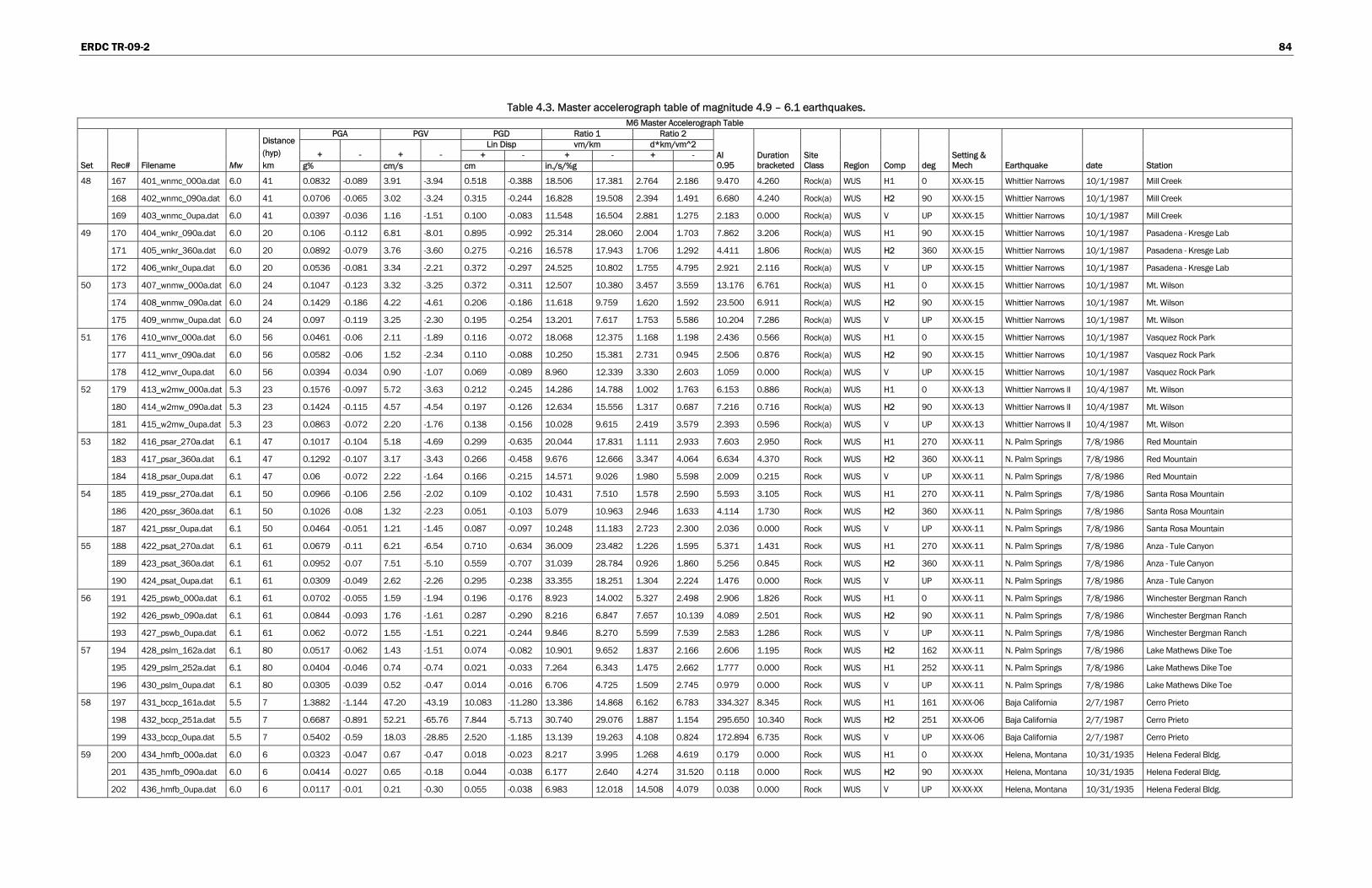
ERDC TR-09-2 84

Table 4.3. Master accelerograph table of magnitude 4.9 – 6.1 earthquakes. M6 Master Accelerograph Table

PGA PGV PGD Ratio 1 Ratio 2 Lin Disp vm/km d*km/vm^2

+ - + - + - + - + - Set Rec# Filename Mw


AI 0.95

Duration bracketed



48 167 401_wnmc_000a.dat 6.0 41 0.0832 -0.089 3.91 -3.94 0.518 -0.388 18.506 17.381 2.764 2.186 9.470 4.260 Rock(a) WUS H1 0 XX-XX-15 Whittier Narrows 10/1/1987 Mill Creek

168 402_wnmc_090a.dat 6.0 41 0.0706 -0.065 3.02 -3.24 0.315 -0.244 16.828 19.508 2.394 1.491 6.680 4.240 Rock(a) WUS H2 90 XX-XX-15 Whittier Narrows 10/1/1987 Mill Creek

169 403_wnmc_0upa.dat 6.0 41 0.0397 -0.036 1.16 -1.51 0.100 -0.083 11.548 16.504 2.881 1.275 2.183 0.000 Rock(a) WUS V UP XX-XX-15 Whittier Narrows 10/1/1987 Mill Creek

49 170 404_wnkr_090a.dat 6.0 20 0.106 -0.112 6.81 -8.01 0.895 -0.992 25.314 28.060 2.004 1.703 7.862 3.206 Rock(a) WUS H1 90 XX-XX-15 Whittier Narrows 10/1/1987 Pasadena - Kresge Lab

171 405_wnkr_360a.dat 6.0 20 0.0892 -0.079 3.76 -3.60 0.275 -0.216 16.578 17.943 1.706 1.292 4.411 1.806 Rock(a) WUS H2 360 XX-XX-15 Whittier Narrows 10/1/1987 Pasadena - Kresge Lab

172 406_wnkr_0upa.dat 6.0 20 0.0536 -0.081 3.34 -2.21 0.372 -0.297 24.525 10.802 1.755 4.795 2.921 2.116 Rock(a) WUS V UP XX-XX-15 Whittier Narrows 10/1/1987 Pasadena - Kresge Lab

50 173 407_wnmw_000a.dat 6.0 24 0.1047 -0.123 3.32 -3.25 0.372 -0.311 12.507 10.380 3.457 3.559 13.176 6.761 Rock(a) WUS H1 0 XX-XX-15 Whittier Narrows 10/1/1987 Mt. Wilson

174 408_wnmw_090a.dat 6.0 24 0.1429 -0.186 4.22 -4.61 0.206 -0.186 11.618 9.759 1.620 1.592 23.500 6.911 Rock(a) WUS H2 90 XX-XX-15 Whittier Narrows 10/1/1987 Mt. Wilson

175 409_wnmw_0upa.dat 6.0 24 0.097 -0.119 3.25 -2.30 0.195 -0.254 13.201 7.617 1.753 5.586 10.204 7.286 Rock(a) WUS V UP XX-XX-15 Whittier Narrows 10/1/1987 Mt. Wilson

51 176 410_wnvr_000a.dat 6.0 56 0.0461 -0.06 2.11 -1.89 0.116 -0.072 18.068 12.375 1.168 1.198 2.436 0.566 Rock(a) WUS H1 0 XX-XX-15 Whittier Narrows 10/1/1987 Vasquez Rock Park

177 411_wnvr_090a.dat 6.0 56 0.0582 -0.06 1.52 -2.34 0.110 -0.088 10.250 15.381 2.731 0.945 2.506 0.876 Rock(a) WUS H2 90 XX-XX-15 Whittier Narrows 10/1/1987 Vasquez Rock Park

178 412_wnvr_0upa.dat 6.0 56 0.0394 -0.034 0.90 -1.07 0.069 -0.089 8.960 12.339 3.330 2.603 1.059 0.000 Rock(a) WUS V UP XX-XX-15 Whittier Narrows 10/1/1987 Vasquez Rock Park

52 179 413_w2mw_000a.dat 5.3 23 0.1576 -0.097 5.72 -3.63 0.212 -0.245 14.286 14.788 1.002 1.763 6.153 0.886 Rock(a) WUS H1 0 XX-XX-13 Whittier Narrows II 10/4/1987 Mt. Wilson

180 414_w2mw_090a.dat 5.3 23 0.1424 -0.115 4.57 -4.54 0.197 -0.126 12.634 15.556 1.317 0.687 7.216 0.716 Rock(a) WUS H2 90 XX-XX-13 Whittier Narrows II 10/4/1987 Mt. Wilson

181 415_w2mw_0upa.dat 5.3 23 0.0863 -0.072 2.20 -1.76 0.138 -0.156 10.028 9.615 2.419 3.579 2.393 0.596 Rock(a) WUS V UP XX-XX-13 Whittier Narrows II 10/4/1987 Mt. Wilson

53 182 416_psar_270a.dat 6.1 47 0.1017 -0.104 5.18 -4.69 0.299 -0.635 20.044 17.831 1.111 2.933 7.603 2.950 Rock WUS H1 270 XX-XX-11 N. Palm Springs 7/8/1986 Red Mountain

183 417_psar_360a.dat 6.1 47 0.1292 -0.107 3.17 -3.43 0.266 -0.458 9.676 12.666 3.347 4.064 6.634 4.370 Rock WUS H2 360 XX-XX-11 N. Palm Springs 7/8/1986 Red Mountain

184 418_psar_0upa.dat 6.1 47 0.06 -0.072 2.22 -1.64 0.166 -0.215 14.571 9.026 1.980 5.598 2.009 0.215 Rock WUS V UP XX-XX-11 N. Palm Springs 7/8/1986 Red Mountain

54 185 419_pssr_270a.dat 6.1 50 0.0966 -0.106 2.56 -2.02 0.109 -0.102 10.431 7.510 1.578 2.590 5.593 3.105 Rock WUS H1 270 XX-XX-11 N. Palm Springs 7/8/1986 Santa Rosa Mountain

186 420_pssr_360a.dat 6.1 50 0.1026 -0.08 1.32 -2.23 0.051 -0.103 5.079 10.963 2.946 1.633 4.114 1.730 Rock WUS H2 360 XX-XX-11 N. Palm Springs 7/8/1986 Santa Rosa Mountain

187 421_pssr_0upa.dat 6.1 50 0.0464 -0.051 1.21 -1.45 0.087 -0.097 10.248 11.183 2.723 2.300 2.036 0.000 Rock WUS V UP XX-XX-11 N. Palm Springs 7/8/1986 Santa Rosa Mountain

55 188 422_psat_270a.dat 6.1 61 0.0679 -0.11 6.21 -6.54 0.710 -0.634 36.009 23.482 1.226 1.595 5.371 1.431 Rock WUS H1 270 XX-XX-11 N. Palm Springs 7/8/1986 Anza - Tule Canyon

189 423_psat_360a.dat 6.1 61 0.0952 -0.07 7.51 -5.10 0.559 -0.707 31.039 28.784 0.926 1.860 5.256 0.845 Rock WUS H2 360 XX-XX-11 N. Palm Springs 7/8/1986 Anza - Tule Canyon

190 424_psat_0upa.dat 6.1 61 0.0309 -0.049 2.62 -2.26 0.295 -0.238 33.355 18.251 1.304 2.224 1.476 0.000 Rock WUS V UP XX-XX-11 N. Palm Springs 7/8/1986 Anza - Tule Canyon

56 191 425_pswb_000a.dat 6.1 61 0.0702 -0.055 1.59 -1.94 0.196 -0.176 8.923 14.002 5.327 2.498 2.906 1.826 Rock WUS H1 0 XX-XX-11 N. Palm Springs 7/8/1986 Winchester Bergman Ranch

192 426_pswb_090a.dat 6.1 61 0.0844 -0.093 1.76 -1.61 0.287 -0.290 8.216 6.847 7.657 10.139 4.089 2.501 Rock WUS H2 90 XX-XX-11 N. Palm Springs 7/8/1986 Winchester Bergman Ranch

193 427_pswb_0upa.dat 6.1 61 0.062 -0.072 1.55 -1.51 0.221 -0.244 9.846 8.270 5.599 7.539 2.583 1.286 Rock WUS V UP XX-XX-11 N. Palm Springs 7/8/1986 Winchester Bergman Ranch

57 194 428_pslm_162a.dat 6.1 80 0.0517 -0.062 1.43 -1.51 0.074 -0.082 10.901 9.652 1.837 2.166 2.606 1.195 Rock WUS H2 162 XX-XX-11 N. Palm Springs 7/8/1986 Lake Mathews Dike Toe

195 429_pslm_252a.dat 6.1 80 0.0404 -0.046 0.74 -0.74 0.021 -0.033 7.264 6.343 1.475 2.662 1.777 0.000 Rock WUS H1 252 XX-XX-11 N. Palm Springs 7/8/1986 Lake Mathews Dike Toe

196 430_pslm_0upa.dat 6.1 80 0.0305 -0.039 0.52 -0.47 0.014 -0.016 6.706 4.725 1.509 2.745 0.979 0.000 Rock WUS V UP XX-XX-11 N. Palm Springs 7/8/1986 Lake Mathews Dike Toe

58 197 431_bccp_161a.dat 5.5 7 1.3882 -1.144 47.20 -43.19 10.083 -11.280 13.386 14.868 6.162 6.783 334.327 8.345 Rock WUS H1 161 XX-XX-06 Baja California 2/7/1987 Cerro Prieto

198 432_bccp_251a.dat 5.5 7 0.6687 -0.891 52.21 -65.76 7.844 -5.713 30.740 29.076 1.887 1.154 295.650 10.340 Rock WUS H2 251 XX-XX-06 Baja California 2/7/1987 Cerro Prieto

199 433_bccp_0upa.dat 5.5 7 0.5402 -0.59 18.03 -28.85 2.520 -1.185 13.139 19.263 4.108 0.824 172.894 6.735 Rock WUS V UP XX-XX-06 Baja California 2/7/1987 Cerro Prieto

59 200 434_hmfb_000a.dat 6.0 6 0.0323 -0.047 0.67 -0.47 0.018 -0.023 8.217 3.995 1.268 4.619 0.179 0.000 Rock WUS H1 0 XX-XX-XX Helena, Montana 10/31/1935 Helena Federal Bldg.

201 435_hmfb_090a.dat 6.0 6 0.0414 -0.027 0.65 -0.18 0.044 -0.038 6.177 2.640 4.274 31.520 0.118 0.000 Rock WUS H2 90 XX-XX-XX Helena, Montana 10/31/1935 Helena Federal Bldg.

202 436_hmfb_0upa.dat 6.0 6 0.0117 -0.01 0.21 -0.30 0.055 -0.038 6.983 12.018 14.508 4.079 0.038 0.000 Rock WUS V UP XX-XX-XX Helena, Montana 10/31/1935 Helena Federal Bldg.

ERDC TR-09-2 85

M6 Master Accelerograph Table PGA PGV PGD Ratio 1 Ratio 2




AI 0.95

Duration bracketed



60 203 437_s7gg_010a.dat 5.3 14 0.0934 -0.095 3.91 -2.16 0.187 -0.181 16.468 8.936 1.124 3.620 2.704 0.426 Rock WUS H1 10 XX-XX-08 San Francisco 3/22/1957 Golden Gate Park

204 438_s7gg_100a.dat 5.3 14 0.1118 -0.101 4.14 -4.58 0.432 -0.310 14.569 17.864 2.766 1.464 4.978 1.611 Rock WUS H2 100 XX-XX-08 San Francisco 3/22/1957 Golden Gate Park

205 439_s7gg_0upa.dat 5.3 14 0.0305 -0.047 1.09 -1.08 0.181 -0.134 14.118 9.020 4.525 5.334 0.667 0.000 Rock WUS V UP XX-XX-08 San Francisco 3/22/1957 Golden Gate Park

61 206 440_smcd_155a.dat 5.6 22 0.2963 -0.302 13.00 -14.87 1.604 -2.004 17.267 19.388 2.760 2.684 39.092 4.139 Rock WUS H1 155 XX-XX-12 Sierra Madre 6/28/1991 Cogswell Dam - Right Abutment

207 441_smcd_065a.dat 5.6 22 0.2641 -0.212 9.55 -7.99 0.579 -0.940 14.244 14.827 1.642 3.063 27.867 3.039 Rock WUS H2 65 XX-XX-12 Sierra Madre 6/28/1991 Cogswell Dam - Right Abutment

208 442_smcd_0upa.dat 5.6 22 0.1665 -0.228 6.09 -6.56 0.772 -0.445 14.394 11.347 3.400 2.311 19.435 3.379 Rock WUS V UP XX-XX-12 Sierra Madre 6/28/1991 Cogswell Dam - Right Abutment

62 209 443_hhg1_157a.dat 5.1 13 0.1054 -0.061 2.55 -2.71 0.089 -0.128 9.533 17.556 1.405 1.042 3.065 1.235 Rock WUS H1 157 XX-XX-06 Hollister 11/28/1974 Gillroy Array # 1

210 444_hhg1_247a.dat 5.1 13 0.1325 -0.084 3.99 -2.71 0.128 -0.168 11.859 12.673 1.045 1.886 4.168 1.100 Rock WUS H2 247 XX-XX-06 Hollister 11/28/1974 Gillroy Array # 1

63 211 445_oror_037a.dat 5.9 14 0.0775 -0.092 2.03 -3.70 0.169 -0.168 10.302 15.854 3.121 1.104 3.230 0.600 Rock WUS H1 37 XX-XX-06 Orville 8/1/1975 Oroville Seismograph

212 446_oror_307a.dat 5.9 14 0.0684 -0.072 2.84 -2.49 0.223 -0.214 16.364 13.548 1.853 2.446 3.581 1.425 Rock WUS H2 307 XX-XX-06 Orville 8/1/1975 Oroville Seismograph

64 213 447_clcd_160a.dat 5.7 11 0.1402 -0.157 10.80 -8.20 0.809 -1.306 30.332 20.505 0.953 2.999 17.005 3.162 Rock WUS H1 160 XX-XX-10 Coyote Lake 8/6/1979 Coyote Lake Dam(SW ABut)

214 448_clcd_250a.dat 5.7 11 0.2791 -0.259 14.18 -20.29 2.331 -1.896 20.002 30.839 3.173 1.170 32.313 3.992 Rock WUS H2 250 XX-XX-10 Coyote Lake 8/6/1979 Coyote Lake Dam(SW ABut)

215 449_clcd_0upa.dat 5.7 11 0.1212 -0.071 6.44 -4.16 0.384 -0.674 20.896 23.117 1.103 2.704 5.218 2.612 Rock WUS V UP XX-XX-10 Coyote Lake 8/6/1979 Coyote Lake Dam(SW ABut)

65 216 450_c7cm_030a.dat 5.2 37 0.085 -0.115 2.29 -3.10 0.092 -0.096 10.589 10.622 1.460 1.119 7.892 2.660 Rock WUS H1 30 XX-XX-21 Northern California 8/6/1979 Cape Mendocino

217 451_c7cm_120a.dat 5.2 37 0.1473 -0.179 4.90 -4.60 0.158 -0.121 13.097 10.121 0.950 1.006 10.688 2.645 Rock WUS H2 120 XX-XX-21 Northern California 8/6/1979 Cape Mendocino

218 452_c7cm_0dna.dat 5.2 37 0.0265 -0.024 0.76 -0.82 0.035 -0.039 11.274 13.652 1.568 1.331 0.702 0.000 Rock WUS V DN XX-XX-21 Northern California 8/6/1979 Cape Mendocino

66 219 453_lccs_095a.dat 5.3 21 0.0708 -0.059 1.80 -1.62 0.098 -0.115 9.993 10.914 2.114 2.503 1.638 0.686 Rock WUS H1 95 XX-XX-08 Lytle Creek 9/12/1970 Cedar Springs - Allen Ranch

220 454_lccs_185a.dat 5.3 21 0.0503 -0.046 1.14 -1.20 0.048 -0.058 8.935 10.228 1.825 1.804 1.065 0.001 Rock WUS H2 185 XX-XX-08 Lytle Creek 9/12/1970 Cedar Springs - Allen Ranch

67 221 455_lcdc_090a.dat 5.3 22 0.1321 -0.146 3.19 -3.33 0.153 -0.181 9.504 8.981 1.946 2.333 8.230 1.630 Rock WUS H1 90 XX-XX-08 Lytle Creek 9/12/1970 Devils Canyon

222 456_lcdc_180a.dat 5.3 22 0.1213 -0.151 4.54 -5.60 0.172 -0.228 14.754 14.598 0.988 1.077 9.388 2.030 Rock WUS H2 180 XX-XX-08 Lytle Creek 9/12/1970 Devils Canyon

223 457_lcdc_0dna.dat 5.3 22 0.0837 -0.08 1.64 -1.73 0.074 -0.101 7.702 8.534 2.258 2.636 1.945 0.260 Rock WUS V DN XX-XX-08 Lytle Creek 9/12/1970 Devils Canyon

68 224 458_lcsa_003a.dat 5.3 46 0.03 -0.042 0.94 -1.64 0.047 -0.095 12.362 15.260 1.566 1.461 0.642 0.000 Rock WUS H1 3 XX-XX-08 Lytle Creek 9/12/1970 Santa Anita Dam

225 459_lcsa_273a.dat 5.3 46 0.0178 -0.018 0.40 -0.50 0.040 -0.035 8.868 10.817 4.360 2.514 0.288 0.000 Rock WUS H2 273 XX-XX-08 Lytle Creek 9/12/1970 Santa Anita Dam

226 460_lcsa_0dna.dat 5.3 46 0.013 -0.013 0.20 -0.27 0.011 -0.011 6.204 8.307 3.358 1.788 0.073 0.000 Rock WUS V DN XX-XX-08 Lytle Creek 9/12/1970 Santa Anita Dam

69 227 461_dtdt_00la.dat 5.3 9 0.2234 -0.199 7.88 -6.72 0.537 -0.459 13.891 13.297 1.894 1.983 16.996 2.630 Rock Turkey H1 L XX-XX-07 Dursunbery, Turkey 7/18/1979 Dursunbery

228 462_dtdt_00ta.dat 5.3 9 0.3662 -0.168 8.11 -10.18 0.577 -0.743 8.714 23.858 3.151 1.181 20.120 2.360 Rock Turkey H2 T XX-XX-07 Dursunbery, Turkey 7/18/1979 Dursunbery

229 463_dtdt_00va.dat 5.3 9 0.127 -0.102 5.72 -4.01 0.309 -0.308 17.733 15.411 1.177 1.928 7.085 2.010 Rock Turkey V V XX-XX-07 Dursunbery, Turkey 7/18/1979 Dursunbery

70 230 464_itiz_00la.dat 5.3 6 0.3297 -0.41 12.46 -10.34 0.452 -0.388 14.877 9.931 0.942 1.460 31.661 1.160 Rock Turkey H L XX-XX-05 Izmir, Turkey 12/16/1977 Izmir

231 465_itiz_00ta.dat 5.3 6 0.1345 -0.146 3.75 -5.33 0.291 -0.203 10.967 14.369 2.737 1.025 5.812 0.720 Rock Turkey H2 T XX-XX-05 Izmir, Turkey 12/16/1977 Izmir

232 466_itiz_00va.dat 5.3 6 0.0707 -0.075 1.61 -2.38 0.065 -0.061 8.967 12.507 1.743 0.796 2.028 1.540 Rock Turkey V V XX-XX-05 Izmir, Turkey 12/16/1977 Izmir

71 233 467_fisr_000a.dat 5.9 18 0.0554 -0.06 4.82 -4.41 1.130 -0.918 34.222 29.082 2.646 2.762 2.958 1.885 Rock Italy H1 0 XX-XX-04 Friuli, Italy 9/15/1976 San Rocco

234 468_fisr_270a.dat 5.9 18 0.1244 -0.134 7.62 -6.27 1.242 -1.994 24.107 18.378 2.610 6.678 7.940 3.175 Rock Italy H2 270 XX-XX-04 Friuli, Italy 9/15/1976 San Rocco

235 469_fisr_0upa.dat 5.9 18 0.0585 -0.05 3.99 -6.23 1.987 -1.309 26.835 49.207 7.171 1.650 2.087 0.020 Rock Italy V UP XX-XX-04 Friuli, Italy 9/15/1976 San Rocco

72 236 470_f2sr_0nsa.dat 5.5 21 0.0282 -0.029 1.41 -2.33 0.478 -0.431 19.750 31.576 6.610 2.257 0.502 0.000 Rock Italy H1 NS XX-XX-06 Friuli, Italy 9/11/1976 San Rocco

237 471_f2sr_0wea.dat 5.5 21 0.0718 -0.045 3.59 -4.31 0.812 -0.543 19.704 38.087 4.426 1.279 1.863 0.091 Rock Italy H2 WE XX-XX-06 Friuli, Italy 9/11/1976 San Rocco

238 472_f2sr_0upa.dat 5.5 21 0.0102 -0.013 1.36 -1.82 0.295 -0.336 52.679 54.365 1.584 1.311 0.227 0.000 Rock Italy V UP XX-XX-06 Friuli, Italy 9/11/1976 San Rocco

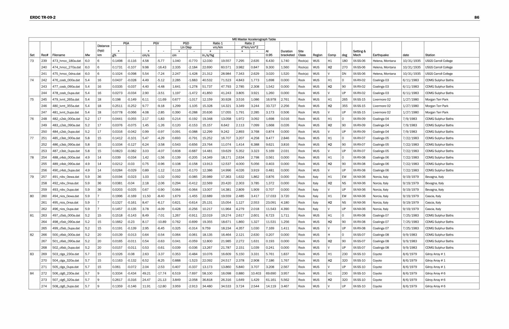
ERDC TR-09-2 86





AI 0.95

Duration bracketed



73 239 473_hmcc_180a.dat 6.0 6 0.1498 -0.116 4.58 -5.77 1.040 -0.770 12.030 19.557 7.295 2.635 6.430 1.740 Rock(a) WUS H1 180 XX-SS-06 Helena, Montana 10/31/1935 USGS Carroll College

240 474_hmcc_270a.dat 6.0 6 0.1731 -0.107 9.98 -16.43 2.335 -2.184 22.690 60.571 3.982 0.847 9.300 1.560 Rock(a) WUS H2 270 XX-SS-06 Helena, Montana 10/31/1935 USGS Carroll College

241 475_hmcc_0dna.dat 6.0 6 0.1024 -0.098 5.54 -7.24 2.247 -1.428 21.312 28.984 7.343 2.629 3.020 1.520 Rock(a) WUS V DN XX-SS-06 Helena, Montana 10/31/1935 USGS Carroll College

74 242 476_cosb_000a.dat 5.4 16 0.0437 -0.028 4.49 -5.12 2.285 -1.683 40.532 71.523 4.843 1.773 1.698 0.000 Rock WUS H1 0 XX-RX-02 Coalinga 03 6/11/1983 CDMG Sulphur Baths

243 477_cosb_090a.dat 5.4 16 0.0335 -0.037 4.40 -4.48 1.641 -1.278 51.737 47.793 2.785 2.308 1.542 0.000 Rock WUS H2 90 XX-RX-02 Coalinga 03 6/11/1983 CDMG Sulphur Baths

244 478_cosb_0upa.dat 5.4 16 0.0273 -0.034 2.90 -3.51 1.197 -1.472 41.850 41.243 3.805 3.921 1.260 0.000 Rock WUS V UP XX-RX-02 Coalinga 03 6/11/1983 CDMG Sulphur Baths

75 245 479_lvmt_265a.dat 5.4 18 0.198 -0.149 6.11 -11.69 0.677 -1.017 12.159 30.928 3.516 1.086 16.978 2.761 Rock WUS H1 265 XX-SS-15 Livermore 02 1/27/1980 Morgan Terr Park

246 480_lvmt_355a.dat 5.4 18 0.2511 -0.252 9.77 -9.18 1.299 -1.105 15.328 14.321 3.349 3.244 33.727 2.256 Rock WUS H2 355 XX-SS-15 Livermore 02 1/27/1980 Morgan Terr Park

247 481_lvmt_0upa.dat 5.4 18 0.0778 -0.066 4.08 -2.85 0.390 -0.288 20.636 17.055 1.791 2.285 3.173 0.506 Rock WUS V UP XX-SS-15 Livermore 02 1/27/1980 Morgan Terr Park

76 248 482_c2sb_000a.dat 5.2 17 0.0441 -0.055 2.17 -1.83 0.214 -0.192 19.348 13.058 1.972 3.092 1.698 0.016 Rock WUS H1 0 XX-RX-09 Coalinga 04 7/9/1983 CDMG Sulphur Baths

249 483_c2sb_090a.dat 5.2 17 0.0376 -0.075 1.45 -1.26 0.120 -0.153 15.157 6.642 2.113 7.099 1.668 0.026 Rock WUS H2 90 XX-RX-09 Coalinga 04 7/9/1983 CDMG Sulphur Baths

250 484_c2sb_0upa.dat 5.2 17 0.0316 -0.042 0.99 -0.97 0.091 -0.088 12.299 9.242 2.893 3.768 0.874 0.000 Rock WUS V UP XX-RX-09 Coalinga 04 7/9/1983 CDMG Sulphur Baths







79 257 491_nibv_0ewa.dat 5.9 36 0.0194 -0.023 1.03 -1.02 0.092 -0.085 20.989 17.363 1.632 1.862 0.876 0.000 Rock Italy H1 EW XX-NX-06 Norcia, Italy 9/19/1979 Bevagna, Italy

258 492_nibv_0nsa.dat 5.9 36 0.0381 -0.04 2.18 -2.06 0.294 -0.412 22.569 20.420 2.303 3.785 1.372 0.000 Rock Italy H2 NS XX-NX-06 Norcia, Italy 9/19/1979 Bevagna, Italy

259 493_nibv_0upa.dat 5.9 36 0.0203 -0.025 0.67 -0.90 0.064 -0.064 13.007 14.381 2.809 1.909 0.707 0.000 Rock Italy V UP XX-NX-06 Norcia, Italy 9/19/1979 Bevagna, Italy

80 260 494_nics_0ewa.dat 5.9 7 0.1996 -0.169 11.50 -8.40 1.679 -1.455 22.689 19.559 2.485 3.417 17.033 3.720 Rock Italy H1 EW XX-NX-06 Norcia, Italy 9/19/1979 Cascia, Italy

261 495_nics_0nsa.dat 5.9 7 0.1327 -0.161 8.47 -6.17 0.621 -0.614 25.131 15.054 1.127 2.553 23.091 4.180 Rock Italy H2 NS XX-NX-06 Norcia, Italy 9/19/1979 Cascia, Italy

262 496_nics_0upa.dat 5.9 7 0.1457 -0.135 3.78 -4.09 0.428 -0.256 10.217 11.964 4.279 2.018 11.543 4.390 Rock Italy V UP XX-NX-06 Norcia, Italy 9/19/1979 Cascia, Italy




82 266 500_c6sb_000a.dat 5.2 20 0.0139 -0.013 0.64 -0.54 0.064 -0.061 18.135 16.464 2.121 2.630 0.207 0.000 Rock WUS H 0 XX-SS-07 Coalinga 08 9/9/1983 CDMG Sulphur Baths

267 501_c6sb_090a.dat 5.2 20 0.0165 -0.011 0.54 -0.63 0.041 -0.059 12.800 21.985 2.272 1.631 0.193 0.000 Rock WUS H2 90 XX-SS-07 Coalinga 08 9/9/1983 CDMG Sulphur Baths

268 502_c6sb_0upa.dat 5.2 20 0.0157 -0.011 0.53 -0.61 0.039 -0.036 13.267 21.787 2.151 1.039 0.241 0.000 Rock WUS V UP XX-SS-07 Coalinga 08 9/9/1983 CDMG Sulphur Baths

83 269 503_clga_230a.dat 5.7 15 0.1026 -0.08 2.63 -3.37 0.353 -0.484 10.076 16.609 5.150 3.331 5.761 1.837 Rock WUS H1 230 XX-SS-10 Coyote 8/6/1979 Gilroy Array # 1

270 504_clga_320a.dat 5.7 15 0.1163 -0.132 6.52 -8.25 0.888 -1.523 22.092 24.517 2.378 2.908 7.186 1.767 Rock WUS H2 320 XX-SS-10 Coyote 8/6/1979 Gilroy Array # 1

271 505_clga_0upa.dat 5.7 15 0.061 -0.072 2.04 -2.53 0.407 -0.337 13.173 13.860 5.840 3.707 3.208 2.567 Rock WUS V UP XX-SS-10 Coyote 8/6/1979 Gilroy Array # 1

84 272 506_clg6_230a.dat 5.7 9 0.3334 -0.434 49.21 -17.74 6.519 -7.697 58.100 16.098 0.880 10.403 69.690 3.957 Rock WUS H1 230 XX-SS-10 Coyote 8/6/1979 Gilroy Array # 6

273 507_clg6_320a.dat 5.7 9 0.2617 -0.316 24.47 -21.13 3.849 -2.058 36.818 26.316 1.649 1.429 61.161 5.562 Rock WUS H2 320 XX-SS-10 Coyote 8/6/1979 Gilroy Array # 6

274 508_clg6_0upa.dat 5.7 9 0.1359 -0.146 11.91 -12.80 3.959 -2.913 34.480 34.533 3.724 2.544 14.119 3.467 Rock WUS V UP XX-SS-10 Coyote 8/6/1979 Gilroy Array # 6

ERDC TR-09-2 87





AI 0.95

Duration bracketed



85 275 509_mlmc_117a.dat 4.9 11 0.0784 -0.075 1.46 -1.62 0.102 -0.087 7.340 8.515 3.683 2.426 2.700 1.326 Rock WUS H 117 XX-XX-08 Mammoth Lakes 09 6/11/1980 USC McGee Creek

276 510_mlmc_207a.dat 4.9 11 0.1936 -0.211 2.97 -2.21 0.077 -0.085 6.046 4.121 1.659 3.614 9.212 0.701 Rock WUS H2 207 XX-XX-08 Mammoth Lakes 09 6/11/1980 USC McGee Creek

277 511_mlmc_0upa.dat 4.9 11 0.0904 -0.066 0.74 -0.76 0.035 -0.024 3.234 4.509 5.599 2.758 1.847 0.946 Rock WUS V UP XX-XX-08 Mammoth Lakes 09 6/11/1980 USC McGee Creek

86 278 512_azpf_045a.dat 5.2 19 0.1099 -0.086 1.71 -2.49 0.105 -0.110 6.141 11.419 3.844 1.492 2.417 1.000 Rock WUS H 45 XX-SS-14 Anza 2/25/1980 Pinyon Flat

279 513_azpf_135a.dat 5.2 19 0.107 -0.131 3.22 -5.11 0.492 -0.368 11.834 15.331 4.988 1.814 3.095 0.835 Rock WUS H2 135 XX-SS-14 Anza 2/25/1980 Pinyon Flat

280 514_azpf_0upa.dat 5.2 19 0.0459 -0.042 0.81 -1.11 0.064 -0.085 6.905 10.318 4.458 2.864 1.206 0.000 Rock WUS V UP XX-SS-14 Anza 2/25/1980 Pinyon Flat

87 281 515_scsl_234a.dat 6.0 76 0.036 -0.035 2.68 -2.94 0.655 -0.973 29.232 33.030 3.233 3.866 1.646 0.000 Rock WUS H 234 XX-XX-XX Southern Cal 11/22/1952 San Luis Obispo

282 516_scsl_324a.dat 6.0 76 0.0441 -0.054 2.57 -3.33 0.531 -0.470 22.951 24.490 3.469 2.227 2.083 0.021 Rock WUS H2 324 XX-XX-XX Southern Cal 11/22/1952 San Luis Obispo

283 517_scsl_0upa.dat 6.0 76 0.0275 -0.021 2.37 -1.60 0.671 -0.411 33.814 30.543 3.236 3.247 0.574 0.000 Rock WUS V UP XX-XX-XX Southern Cal 11/22/1952 San Luis Obispo

88 284 518_aztv_045a.dat 5.2 16 0.1283 -0.131 3.92 -2.80 0.166 -0.123 12.015 8.396 1.360 2.030 3.993 0.625 Rock WUS H 45 XX-SS-14 Anza 2/25/1980 Terwilliger Valley

285 519_aztv_135a.dat 5.2 16 0.0805 -0.079 1.67 -1.64 0.064 -0.064 8.181 8.223 1.803 1.824 1.980 0.705 Rock WUS H2 135 XX-SS-14 Anza 2/25/1980 Terwilliger Valley

286 520_aztv_0upa.dat 5.2 16 0.0678 -0.066 1.66 -1.29 0.057 -0.057 9.656 7.662 1.367 2.226 1.479 0.640 Rock WUS V UP XX-SS-14 Anza 2/25/1980 Terwilliger Valley

89 287 521_bb7r_090a.dat 4.9 33 0.0113 -0.011 0.31 -0.31 0.063 -0.067 10.699 11.048 7.399 7.667 0.094 0.000 Rock WUS H 90 XX-SS-06 Big Bear City 2/22/2003 Seven Oaks Dam Right Abut

288 522_bb7r_360a.dat 4.9 33 0.013 -0.012 0.45 -0.43 0.089 -0.091 13.686 14.132 5.553 5.789 0.115 0.000 Rock WUS H2 360 XX-SS-06 Big Bear City 2/22/2003 Seven Oaks Dam Right Abut

289 523_bb7r_0upa.dat 4.9 33 0.0081 -0.008 0.27 -0.23 0.020 -0.029 13.357 11.073 2.138 4.442 0.065 0.000 Rock WUS V UP XX-SS-06 Big Bear City 2/22/2003 Seven Oaks Dam Right Abut

90 290 524_bb7d_090a.dat 4.9 33 0.027 -0.031 0.77 -0.66 0.073 -0.081 11.251 8.462 3.260 5.558 0.633 0.000 Rock WUS H 90 XX-SS-06 Big Bear City 2/22/2003 Seven Oaks Dam Downstream

291 525_bb7d_360a.dat 4.9 33 0.0419 -0.03 0.77 -0.86 0.072 -0.081 7.268 11.231 4.958 3.228 0.648 0.000 Rock WUS H2 360 XX-SS-06 Big Bear City 2/22/2003 Seven Oaks Dam Downstream

292 526_bb7d_0upa.dat 4.9 33 0.0125 -0.012 0.22 -0.25 0.021 -0.024 6.875 8.123 5.488 4.613 0.143 0.000 Rock WUS V UP XX-SS-06 Big Bear City 2/22/2003 Seven Oaks Dam Downstream

91 293 527_bbsb_111a.dat 4.9 41 0.0064 -0.007 0.41 -0.33 0.055 -0.083 25.002 18.420 2.081 5.211 0.078 0.000 Rock WUS H 111 XX-SS-06 Big Bear City 2/22/2003 San Bernardino - Del Rosa

294 528_bbsb_021a.dat 4.9 41 0.0082 -0.008 0.38 -0.36 0.093 -0.123 18.173 19.237 5.234 6.740 0.087 0.000 Rock WUS H2 21 XX-SS-06 Big Bear City 2/22/2003 San Bernardino - Del Rosa

295 529_bbsb_0upa.dat 4.9 41 0.0062 -0.007 0.19 -0.24 0.036 -0.045 11.835 14.053 6.198 5.280 0.047 0.000 Rock WUS V UP XX-SS-06 Big Bear City 2/22/2003 San Bernardino - Del Rosa

92 296 530_lzat_0nsa.dat 5.8 19 0.0933 -0.061 3.33 -3.29 0.417 -0.437 14.059 21.150 3.437 2.425 5.515 2.111 Rock Italy H NS XX-XX-14 Lazio-Abruzzo 5/7/1984 ENEL 99999 Atina, Italy

297 531_lzat_0wea.dat 5.8 19 0.1135 -0.07 3.77 -4.00 0.345 -0.337 13.084 22.446 2.700 1.450 4.677 1.252 Rock Italy H2 WE XX-XX-14 Lazio-Abruzzo 5/7/1984 ENEL 99999 Atina, Italy

298 532_lzat_0upa.dat 5.8 19 0.0757 -0.046 1.75 -2.03 0.234 -0.263 9.105 17.227 5.656 2.910 3.096 0.035 Rock Italy V UP XX-XX-14 Lazio-Abruzzo 5/7/1984 ENEL 99999 Atina, Italy

93 299 533_h4ss_205a.dat 5.5 14 0.0439 -0.044 5.32 -5.03 1.266 -0.847 47.688 45.232 1.925 1.437 2.270 0.000 Rock WUS H 205 XX-SS-09 Hollister-04 1/26/1980 SAGO South - Surface

300 534_h4ss_295a.dat 5.5 14 0.0615 -0.09 4.96 -9.26 1.500 -1.698 31.735 40.546 3.683 1.745 4.619 1.276 Rock WUS H2 295 XX-SS-09 Hollister-04 1/26/1980 SAGO South - Surface

301 535_h4ss_0upa.dat 5.5 14 0.0305 -0.053 3.27 -3.38 0.529 -0.388 42.260 25.143 1.477 1.764 1.692 0.026 Rock WUS V UP XX-SS-09 Hollister-04 1/26/1980 SAGO South - Surface

94 302 536_pgpk_0nsa.dat 5.0 176 0.1499 -0.157 8.04 -8.03 0.541 -0.496 21.116 20.171 1.230 1.183 19.937 4.311 Rock Greece H NS XX-XX-81 Pelekanada 10/10/1984 ITSAK Pelekanada, Greece

303 537_pgpk_0wea.dat 5.0 176 0.1489 -0.168 7.80 -6.29 0.532 -0.481 20.638 14.750 1.274 2.001 20.317 3.814 Rock Greece H2 WE XX-XX-81 Pelekanada 10/10/1984 ITSAK Pelekanada, Greece

304 538_pgpk_0upa.dat 5.0 176 0.0834 -0.102 2.87 -2.93 0.175 -0.159 13.553 11.377 1.734 1.840 9.199 4.755 Rock Greece V UP XX-XX-81 Pelekanada 10/10/1984 ITSAK Pelekanada, Greece

95 305 539_dgkv_0nsa.dat 5.2 48 0.0398 -0.049 2.25 -1.83 0.105 -0.106 22.230 14.849 0.807 1.504 1.836 0.000 Rock Greece H NS XX-SS-14 Drama 11/9/1985 ITSAK Kavala

306 540_dgkv_0wea.dat 5.2 48 0.0387 -0.036 1.37 -1.20 0.082 -0.065 13.958 13.145 1.648 1.605 1.374 0.000 Rock Greece H2 WE XX-SS-14 Drama 11/9/1985 ITSAK Kavala

307 541_dgkv_0upa.dat 5.2 48 0.0491 -0.031 1.51 -1.11 0.090 -0.071 12.093 14.185 1.899 1.757 0.791 0.000 Rock Greece V UP XX-SS-14 Drama 11/9/1985 ITSAK Kavala

96 308 542_cc38_00ea.dat 5.9 64 0.009 -0.007 0.60 -0.75 0.131 -0.140 26.097 43.212 3.239 1.664 0.111 0.000 Rock Taiwan H E XX-XX-08 Chi-Chi 9/20/1999 CWB HWA 038, Taiwan

309 543_cc38_00na.dat 5.9 64 0.0125 -0.01 1.03 -0.73 0.192 -0.164 32.429 27.915 2.223 3.128 0.154 0.000 Rock Taiwan H2 N XX-XX-08 Chi-Chi 9/20/1999 CWB HWA 038, Taiwan

310 544_cc38_00va.dat 5.9 64 0.0085 -0.007 0.68 -0.42 0.115 -0.104 31.511 24.380 2.060 3.918 0.106 0.000 Rock Taiwan V V XX-XX-08 Chi-Chi 9/20/1999 CWB HWA 038, Taiwan

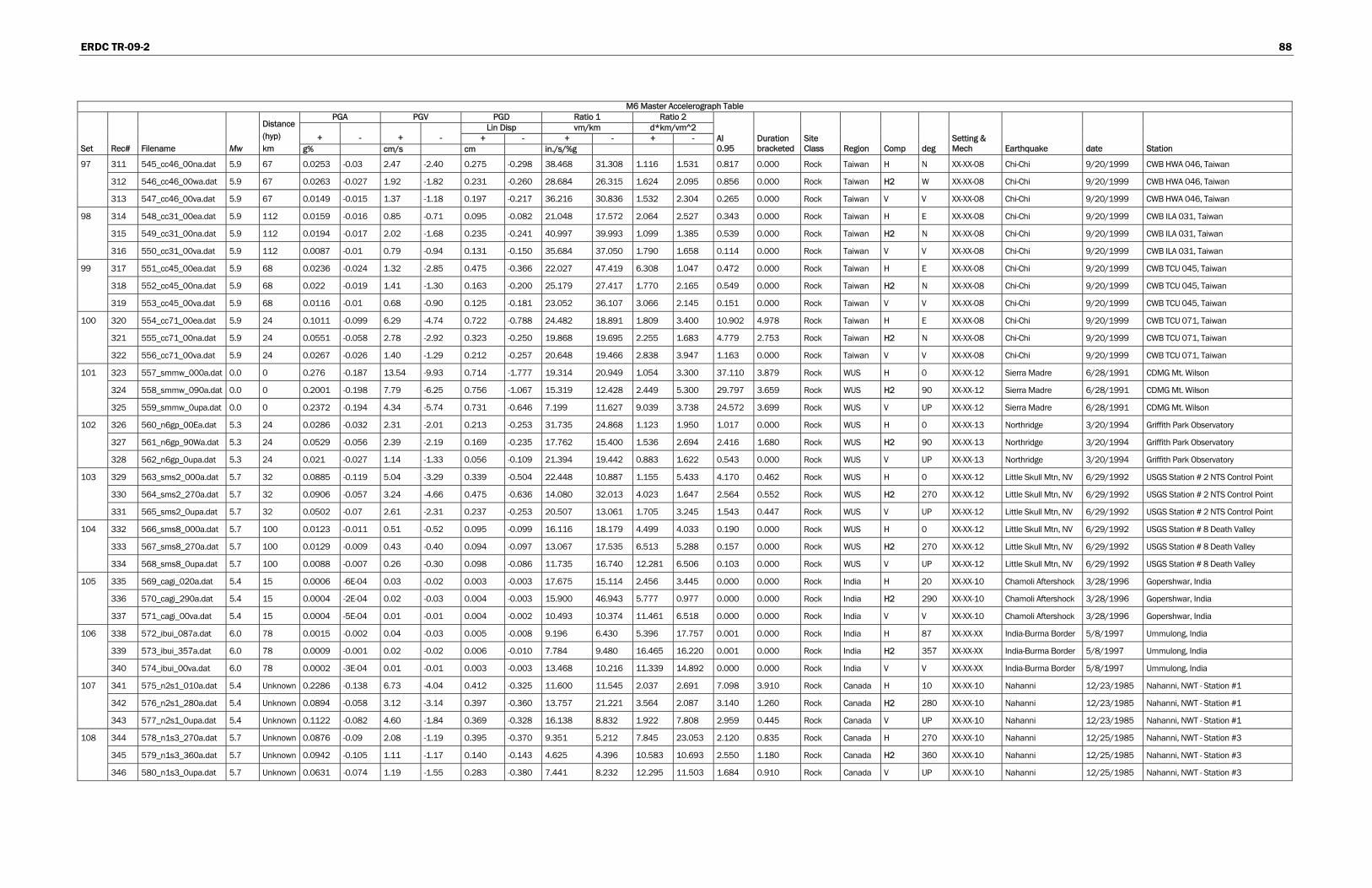
ERDC TR-09-2 88





AI 0.95

Duration bracketed



97 311 545_cc46_00na.dat 5.9 67 0.0253 -0.03 2.47 -2.40 0.275 -0.298 38.468 31.308 1.116 1.531 0.817 0.000 Rock Taiwan H N XX-XX-08 Chi-Chi 9/20/1999 CWB HWA 046, Taiwan

312 546_cc46_00wa.dat 5.9 67 0.0263 -0.027 1.92 -1.82 0.231 -0.260 28.684 26.315 1.624 2.095 0.856 0.000 Rock Taiwan H2 W XX-XX-08 Chi-Chi 9/20/1999 CWB HWA 046, Taiwan

313 547_cc46_00va.dat 5.9 67 0.0149 -0.015 1.37 -1.18 0.197 -0.217 36.216 30.836 1.532 2.304 0.265 0.000 Rock Taiwan V V XX-XX-08 Chi-Chi 9/20/1999 CWB HWA 046, Taiwan

98 314 548_cc31_00ea.dat 5.9 112 0.0159 -0.016 0.85 -0.71 0.095 -0.082 21.048 17.572 2.064 2.527 0.343 0.000 Rock Taiwan H E XX-XX-08 Chi-Chi 9/20/1999 CWB ILA 031, Taiwan

315 549_cc31_00na.dat 5.9 112 0.0194 -0.017 2.02 -1.68 0.235 -0.241 40.997 39.993 1.099 1.385 0.539 0.000 Rock Taiwan H2 N XX-XX-08 Chi-Chi 9/20/1999 CWB ILA 031, Taiwan

316 550_cc31_00va.dat 5.9 112 0.0087 -0.01 0.79 -0.94 0.131 -0.150 35.684 37.050 1.790 1.658 0.114 0.000 Rock Taiwan V V XX-XX-08 Chi-Chi 9/20/1999 CWB ILA 031, Taiwan

99 317 551_cc45_00ea.dat 5.9 68 0.0236 -0.024 1.32 -2.85 0.475 -0.366 22.027 47.419 6.308 1.047 0.472 0.000 Rock Taiwan H E XX-XX-08 Chi-Chi 9/20/1999 CWB TCU 045, Taiwan

318 552_cc45_00na.dat 5.9 68 0.022 -0.019 1.41 -1.30 0.163 -0.200 25.179 27.417 1.770 2.165 0.549 0.000 Rock Taiwan H2 N XX-XX-08 Chi-Chi 9/20/1999 CWB TCU 045, Taiwan

319 553_cc45_00va.dat 5.9 68 0.0116 -0.01 0.68 -0.90 0.125 -0.181 23.052 36.107 3.066 2.145 0.151 0.000 Rock Taiwan V V XX-XX-08 Chi-Chi 9/20/1999 CWB TCU 045, Taiwan

100 320 554_cc71_00ea.dat 5.9 24 0.1011 -0.099 6.29 -4.74 0.722 -0.788 24.482 18.891 1.809 3.400 10.902 4.978 Rock Taiwan H E XX-XX-08 Chi-Chi 9/20/1999 CWB TCU 071, Taiwan

321 555_cc71_00na.dat 5.9 24 0.0551 -0.058 2.78 -2.92 0.323 -0.250 19.868 19.695 2.255 1.683 4.779 2.753 Rock Taiwan H2 N XX-XX-08 Chi-Chi 9/20/1999 CWB TCU 071, Taiwan

322 556_cc71_00va.dat 5.9 24 0.0267 -0.026 1.40 -1.29 0.212 -0.257 20.648 19.466 2.838 3.947 1.163 0.000 Rock Taiwan V V XX-XX-08 Chi-Chi 9/20/1999 CWB TCU 071, Taiwan

101 323 557_smmw_000a.dat 0.0 0 0.276 -0.187 13.54 -9.93 0.714 -1.777 19.314 20.949 1.054 3.300 37.110 3.879 Rock WUS H 0 XX-XX-12 Sierra Madre 6/28/1991 CDMG Mt. Wilson

324 558_smmw_090a.dat 0.0 0 0.2001 -0.198 7.79 -6.25 0.756 -1.067 15.319 12.428 2.449 5.300 29.797 3.659 Rock WUS H2 90 XX-XX-12 Sierra Madre 6/28/1991 CDMG Mt. Wilson

325 559_smmw_0upa.dat 0.0 0 0.2372 -0.194 4.34 -5.74 0.731 -0.646 7.199 11.627 9.039 3.738 24.572 3.699 Rock WUS V UP XX-XX-12 Sierra Madre 6/28/1991 CDMG Mt. Wilson

102 326 560_n6gp_00Ea.dat 5.3 24 0.0286 -0.032 2.31 -2.01 0.213 -0.253 31.735 24.868 1.123 1.950 1.017 0.000 Rock WUS H 0 XX-XX-13 Northridge 3/20/1994 Griffith Park Observatory

327 561_n6gp_90Wa.dat 5.3 24 0.0529 -0.056 2.39 -2.19 0.169 -0.235 17.762 15.400 1.536 2.694 2.416 1.680 Rock WUS H2 90 XX-XX-13 Northridge 3/20/1994 Griffith Park Observatory

328 562_n6gp_0upa.dat 5.3 24 0.021 -0.027 1.14 -1.33 0.056 -0.109 21.394 19.442 0.883 1.622 0.543 0.000 Rock WUS V UP XX-XX-13 Northridge 3/20/1994 Griffith Park Observatory

103 329 563_sms2_000a.dat 5.7 32 0.0885 -0.119 5.04 -3.29 0.339 -0.504 22.448 10.887 1.155 5.433 4.170 0.462 Rock WUS H 0 XX-XX-12 Little Skull Mtn, NV 6/29/1992 USGS Station # 2 NTS Control Point

330 564_sms2_270a.dat 5.7 32 0.0906 -0.057 3.24 -4.66 0.475 -0.636 14.080 32.013 4.023 1.647 2.564 0.552 Rock WUS H2 270 XX-XX-12 Little Skull Mtn, NV 6/29/1992 USGS Station # 2 NTS Control Point

331 565_sms2_0upa.dat 5.7 32 0.0502 -0.07 2.61 -2.31 0.237 -0.253 20.507 13.061 1.705 3.245 1.543 0.447 Rock WUS V UP XX-XX-12 Little Skull Mtn, NV 6/29/1992 USGS Station # 2 NTS Control Point

104 332 566_sms8_000a.dat 5.7 100 0.0123 -0.011 0.51 -0.52 0.095 -0.099 16.116 18.179 4.499 4.033 0.190 0.000 Rock WUS H 0 XX-XX-12 Little Skull Mtn, NV 6/29/1992 USGS Station # 8 Death Valley

333 567_sms8_270a.dat 5.7 100 0.0129 -0.009 0.43 -0.40 0.094 -0.097 13.067 17.535 6.513 5.288 0.157 0.000 Rock WUS H2 270 XX-XX-12 Little Skull Mtn, NV 6/29/1992 USGS Station # 8 Death Valley

334 568_sms8_0upa.dat 5.7 100 0.0088 -0.007 0.26 -0.30 0.098 -0.086 11.735 16.740 12.281 6.506 0.103 0.000 Rock WUS V UP XX-XX-12 Little Skull Mtn, NV 6/29/1992 USGS Station # 8 Death Valley

105 335 569_cagi_020a.dat 5.4 15 0.0006 -6E-04 0.03 -0.02 0.003 -0.003 17.675 15.114 2.456 3.445 0.000 0.000 Rock India H 20 XX-XX-10 Chamoli Aftershock 3/28/1996 Gopershwar, India

336 570_cagi_290a.dat 5.4 15 0.0004 -2E-04 0.02 -0.03 0.004 -0.003 15.900 46.943 5.777 0.977 0.000 0.000 Rock India H2 290 XX-XX-10 Chamoli Aftershock 3/28/1996 Gopershwar, India

337 571_cagi_00va.dat 5.4 15 0.0004 -5E-04 0.01 -0.01 0.004 -0.002 10.493 10.374 11.461 6.518 0.000 0.000 Rock India V V XX-XX-10 Chamoli Aftershock 3/28/1996 Gopershwar, India

106 338 572_ibui_087a.dat 6.0 78 0.0015 -0.002 0.04 -0.03 0.005 -0.008 9.196 6.430 5.396 17.757 0.001 0.000 Rock India H 87 XX-XX-XX India-Burma Border 5/8/1997 Ummulong, India

339 573_ibui_357a.dat 6.0 78 0.0009 -0.001 0.02 -0.02 0.006 -0.010 7.784 9.480 16.465 16.220 0.001 0.000 Rock India H2 357 XX-XX-XX India-Burma Border 5/8/1997 Ummulong, India

340 574_ibui_00va.dat 6.0 78 0.0002 -3E-04 0.01 -0.01 0.003 -0.003 13.468 10.216 11.339 14.892 0.000 0.000 Rock India V V XX-XX-XX India-Burma Border 5/8/1997 Ummulong, India

107 341 575_n2s1_010a.dat 5.4 Unknown 0.2286 -0.138 6.73 -4.04 0.412 -0.325 11.600 11.545 2.037 2.691 7.098 3.910 Rock Canada H 10 XX-XX-10 Nahanni 12/23/1985 Nahanni, NWT - Station #1

342 576_n2s1_280a.dat 5.4 Unknown 0.0894 -0.058 3.12 -3.14 0.397 -0.360 13.757 21.221 3.564 2.087 3.140 1.260 Rock Canada H2 280 XX-XX-10 Nahanni 12/23/1985 Nahanni, NWT - Station #1

343 577_n2s1_0upa.dat 5.4 Unknown 0.1122 -0.082 4.60 -1.84 0.369 -0.328 16.138 8.832 1.922 7.808 2.959 0.445 Rock Canada V UP XX-XX-10 Nahanni 12/23/1985 Nahanni, NWT - Station #1

108 344 578_n1s3_270a.dat 5.7 Unknown 0.0876 -0.09 2.08 -1.19 0.395 -0.370 9.351 5.212 7.845 23.053 2.120 0.835 Rock Canada H 270 XX-XX-10 Nahanni 12/25/1985 Nahanni, NWT - Station #3

345 579_n1s3_360a.dat 5.7 Unknown 0.0942 -0.105 1.11 -1.17 0.140 -0.143 4.625 4.396 10.583 10.693 2.550 1.180 Rock Canada H2 360 XX-XX-10 Nahanni 12/25/1985 Nahanni, NWT - Station #3

346 580_n1s3_0upa.dat 5.7 Unknown 0.0631 -0.074 1.19 -1.55 0.283 -0.380 7.441 8.232 12.295 11.503 1.684 0.910 Rock Canada V UP XX-XX-10 Nahanni 12/25/1985 Nahanni, NWT - Station #3

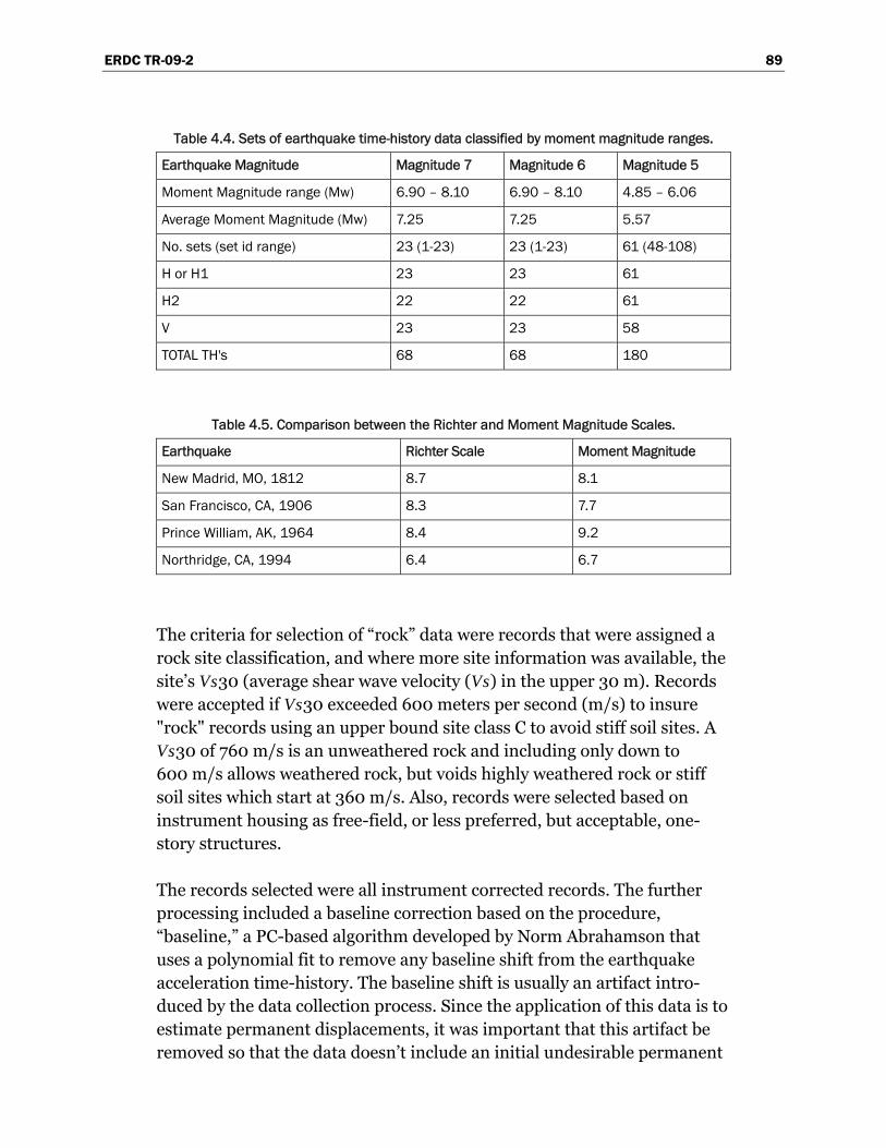
ERDC TR-09-2 89

Table 4.4. Sets of earthquake time-history data classified by moment magnitude ranges.

Earthquake Magnitude Magnitude 7 Magnitude 6 Magnitude 5

Moment Magnitude range (Mw) 6.90 – 8.10 6.90 – 8.10 4.85 – 6.06

Average Moment Magnitude (Mw) 7.25 7.25 5.57

No. sets (set id range) 23 (1-23) 23 (1-23) 61 (48-108)

H or H1 23 23 61

H2 22 22 61

V 23 23 58

TOTAL TH's 68 68 180

Table 4.5. Comparison between the Richter and Moment Magnitude Scales.

Earthquake Richter Scale Moment Magnitude

New Madrid, MO, 1812 8.7 8.1

San Francisco, CA, 1906 8.3 7.7

Prince William, AK, 1964 8.4 9.2

Northridge, CA, 1994 6.4 6.7

The criteria for selection of “rock” data were records that were assigned a rock site classification, and where more site information was available, the site’s Vs30 (average shear wave velocity (Vs) in the upper 30 m). Records were accepted if Vs30 exceeded 600 meters per second (m/s) to insure "rock" records using an upper bound site class C to avoid stiff soil sites. A Vs30 of 760 m/s is an unweathered rock and including only down to 600 m/s allows weathered rock, but voids highly weathered rock or stiff soil sites which start at 360 m/s. Also, records were selected based on instrument housing as free-field, or less preferred, but acceptable, one-story structures.

The records selected were all instrument corrected records. The further processing included a baseline correction based on the procedure, “baseline,” a PC-based algorithm developed by Norm Abrahamson that uses a polynomial fit to remove any baseline shift from the earthquake acceleration time-history. The baseline shift is usually an artifact intro-duced by the data collection process. Since the application of this data is to estimate permanent displacements, it was important that this artifact be removed so that the data doesn’t include an initial undesirable permanent

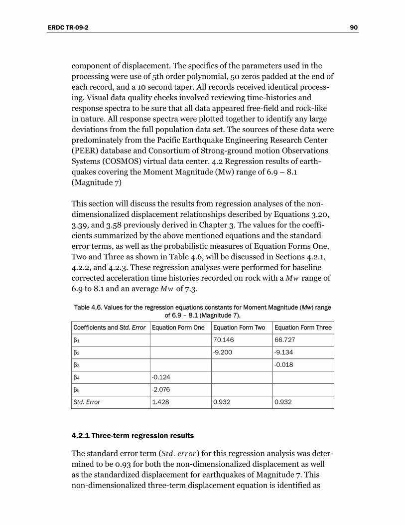
ERDC TR-09-2 90

component of displacement. The specifics of the parameters used in the processing were use of 5th order polynomial, 50 zeros padded at the end of each record, and a 10 second taper. All records received identical process-ing. Visual data quality checks involved reviewing time-histories and response spectra to be sure that all data appeared free-field and rock-like in nature. All response spectra were plotted together to identify any large deviations from the full population data set. The sources of these data were predominately from the Pacific Earthquake Engineering Research Center (PEER) database and Consortium of Strong-ground motion Observations Systems (COSMOS) virtual data center. 4.2 Regression results of earth-quakes covering the Moment Magnitude (Mw) range of 6.9 – 8.1 (Magnitude 7)

This section will discuss the results from regression analyses of the non-dimensionalized displacement relationships described by Equations 3.20, 3.39, and 3.58 previously derived in Chapter 3. The values for the coeffi-cients summarized by the above mentioned equations and the standard error terms, as well as the probabilistic measures of Equation Forms One, Two and Three as shown in Table 4.6, will be discussed in Sections 4.2.1, 4.2.2, and 4.2.3. These regression analyses were performed for baseline corrected acceleration time histories recorded on rock with a Mw range of 6.9 to 8.1 and an average Mw of 7.3.

Table 4.6. Values for the regression equations constants for Moment Magnitude (Mw) range of 6.9 – 8.1 (Magnitude 7).

Coefficients and Std. Error Equation Form One Equation Form Two Equation Form Three

β1 70.146 66.727

β2 -9.200 -9.134

β3 -0.018

β4 -0.124

β5 -2.076

Std. Error 1.428 0.932 0.932

4.2.1 Three-term regression results

The standard error term (Std. error) for this regression analysis was deter-mined to be 0.93 for both the non-dimensionalized displacement as well as the standardized displacement for earthquakes of Magnitude 7. This non-dimensionalized three-term displacement equation is identified as

ERDC TR-09-2 91

Equation Form Three with the coefficients and Std. error terms summa-rized in column four of Table 4.6.

4.2.1.1 Mean relationships

The regression analysis of the 23 sets of Magnitude 7 acceleration time histories resulted in the mean non-dimensionalized displacement rela-tionship of

.

. exp .m m c c

m mm

d k g k kk kv

−⎛ ⎞ ⎛ ⎞• ⎟ ⎟⎜ ⎜⎟ ⎟= • − • •⎜ ⎜⎟ ⎟⎜ ⎜⎟ ⎟⎜ ⎜⎝ ⎠ ⎝ ⎠

0 018

2 66 7 9 13 (4.1)

where:

dm = permanent displacement kmg = peak (positive) rock acceleration expressed in units of length

per sec2, consistent with units of dm (length) and vm (length per sec)

vm = peak (positive) ground velocity of the earthquake kc = critical acceleration expressed as a fraction of g km = peak (positive) rock acceleration expressed as a fraction of g.

This mean relationship is shown in yellow in Figure 4.1.

By a second independent regression analysis, the mean standardized maximum displacement (ds) in units of inches was derived for the stan-dardized velocity, vs = 29.92 in./sec (0.76 m/sec) and the standardized acceleration ks = 0.5 g (193.04 in./sec2 : 4.90 m/sec2)

.

. exp . c cs

m m

k kd

k k

−⎛ ⎞ ⎛ ⎞⎟ ⎟⎜ ⎜⎟ ⎟= • − • •⎜ ⎜⎟ ⎟⎜ ⎜⎟ ⎟⎜ ⎜⎝ ⎠ ⎝ ⎠

0 018

309 5 9 13 (4.2)

The standardized maximum displacement (ds) can be converted to the permanent displacement (dm) by the following transformation (Franklin and Chang 1977),

s mm s

ms

k vd d

kv

⎡ ⎤⎛ ⎞ ⎛ ⎞⎟⎜ ⎜ ⎟⎢ ⎥⎟= • •⎜ ⎜⎟ ⎟⎟⎢ ⎥⎜ ⎜⎟⎜ ⎜⎝ ⎠ ⎝ ⎠⎟⎢ ⎥⎣ ⎦

2

2 (4.3)

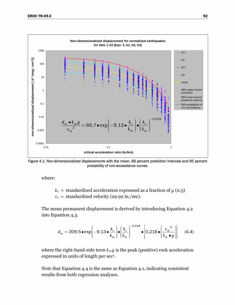
ERDC TR-09-2 92

Non-dimensionalized displacement for normalized earthquakes for Sets 1-23 (Eqn. 3, b1, b2, b3)

0.0001

0.001

0.01

0.1

1

10

100

1000

0.01 0.1 1

critical acceleration ratio (kc/km)

non-

dim

ensi

onal

ized

dis

plac

emen

t [ d

* km

g / v

m^2

]

H1+

H1-

H2+

H2-

mean

68% upper boundprediction

68% lower boundprediction interval

95% probability ofnon exceedance

.

. exp .m m c c

m mm

d k g k kk kv

−⎛ ⎞ ⎛ ⎞• ⎟ ⎟⎜ ⎜⎟ ⎟= • − • •⎜ ⎜⎟ ⎟⎜ ⎜⎟ ⎟⎜ ⎜⎝ ⎠ ⎝ ⎠

0 018

2 66 7 9 13

Figure 4.1. Non-dimensionalized displacements with the mean, 68 percent prediction intervals and 95 percent probability of non-exceedance curves.

where:

ks = standardized acceleration expressed as a fraction of g (0.5) vs = standardized velocity (29.92 in./sec).

The mean permanent displacement is derived by introducing Equation 4.2 into Equation 4.3.

.

. exp . .c c mm

m m m

k k vd

k k k g

− ⎡ ⎤⎛ ⎞⎛ ⎞ ⎛ ⎞ ⎟⎟ ⎟ ⎜⎜ ⎜ ⎢ ⎥⎟⎟ ⎟= • − • • • •⎜⎜ ⎜ ⎟⎟ ⎟ ⎢ ⎥⎜⎜ ⎜ ⎟⎟ ⎟⎜ ⎜ ⎜ •⎝ ⎠ ⎝ ⎠ ⎝ ⎠⎢ ⎥⎣ ⎦

0 018 2

309 5 9 13 0 216 (4.4)

where the right-hand-side term kmg is the peak (positive) rock acceleration expressed in units of length per sec2.

Note that Equation 4.4 is the same as Equation 4.1, indicating consistent results from both regression analyses.

ERDC TR-09-2 93

4.2.1.2 Ninety-five percent probability of non-exceedance

The regression analysis of the 23 sets of Magnitude 7 rock acceleration time histories resulted in the non-dimensionalized displacement for 95 percent probability of non-exceedance of

.

. exp . .m m c c

m mm

d k g k kk kv

−⎛ ⎞ ⎛ ⎞• ⎟ ⎟⎜ ⎜⎟ ⎟= • − • • •⎜ ⎜⎟ ⎟⎜ ⎜⎟ ⎟⎜ ⎜⎝ ⎠ ⎝ ⎠

0 018

2 66 7 9 13 4 64 (4.5)

The 95 percent probability of non-exceedance is shown in red in Figure 4.1.

By the second independent regression analysis, the standardized maxi-mum displacement (ds) in units of inches, derived using vs = 29.92 in./sec and ks = 0.5 g, is

.

. exp . c cs

m m

k kd

k k

−⎛ ⎞ ⎛ ⎞⎟ ⎟⎜ ⎜⎟ ⎟= • − • • •⎜ ⎜⎟ ⎟⎜ ⎜⎟ ⎟⎜ ⎜⎝ ⎠ ⎝ ⎠

0 018

309 5 9 13 4 64. (4.6)

The corresponding permanent displacement is

.

. exp . . .c c mm

m m m

k k vd

k k k g

− ⎡ ⎤⎛ ⎞⎛ ⎞ ⎛ ⎞ ⎟⎟ ⎟ ⎜⎜ ⎜ ⎢ ⎥⎟⎟ ⎟= • − • • • • •⎜⎜ ⎜ ⎟⎟ ⎟ ⎢ ⎥⎜⎜ ⎜ ⎟⎟ ⎟⎜ ⎜ ⎜ •⎝ ⎠ ⎝ ⎠ ⎝ ⎠⎢ ⎥⎣ ⎦

0 018 2

309 5 9 13 4 64 0 216 (4.7)

Note that Equation 4.7 is the same as Equation 4.5, indicating consistent results from both regression analyses,

4.2.1.3 Sixty-eight percent prediction intervals

The regression analysis of the 23 sets of Magnitude 7 rock acceleration time histories resulted in the non-dimensionalized displacement relation-ships for the 68 percent prediction intervals of

.

. exp . .m m c c

m mm

d k g k kk kv

−⎛ ⎞ ⎛ ⎞• ⎟ ⎟⎜ ⎜⎟ ⎟= • − • • •⎜ ⎜⎟ ⎟⎜ ⎜⎟ ⎟⎜ ⎜⎝ ⎠ ⎝ ⎠

0 018

2 66 7 9 13 2 53 (4.8a)

.

. exp . .m m c c

m mm

d k g k kk kv

−⎛ ⎞ ⎛ ⎞• ⎟ ⎟⎜ ⎜⎟ ⎟= • − • • •⎜ ⎜⎟ ⎟⎜ ⎜⎟ ⎟⎜ ⎜⎝ ⎠ ⎝ ⎠

0 018

2 66 7 9 13 0 39 (4.8b)

ERDC TR-09-2 94

The 68 percent prediction intervals are shown in blue in Figure 4.1.

By the second independent regression analysis, the standardized maxi-mum displacements (ds) in units of inches, derived using vs = 29.92 in./sec and ks = 0.5 g, are

.

. exp . .c cs

m m

k kd

k k

−⎛ ⎞ ⎛ ⎞⎟ ⎟⎜ ⎜⎟ ⎟= • − • • •⎜ ⎜⎟ ⎟⎜ ⎜⎟ ⎟⎜ ⎜⎝ ⎠ ⎝ ⎠

0 018

309 5 9 13 2 53 (4.9a)

.

. exp . c cs

m m

k kd

k k

−⎛ ⎞ ⎛ ⎞⎟ ⎟⎜ ⎜⎟ ⎟= • − • • •⎜ ⎜⎟ ⎟⎜ ⎜⎟ ⎟⎜ ⎜⎝ ⎠ ⎝ ⎠

0 018

309 5 9 13 0 39. (4.9b)

Introducing Equation 4.3, the corresponding permanent displacements are

.

. exp . . .c c mm

m m m

k k vd

k k k g

− ⎡ ⎤⎛ ⎞⎛ ⎞ ⎛ ⎞ ⎟⎟ ⎟ ⎜⎜ ⎜ ⎢ ⎥⎟⎟ ⎟= • − • • • • •⎜⎜ ⎜ ⎟⎟ ⎟ ⎢ ⎥⎜⎜ ⎜ ⎟⎟ ⎟⎜ ⎜ ⎜ •⎝ ⎠ ⎝ ⎠ ⎝ ⎠⎢ ⎥⎣ ⎦

0 018 2

309 5 9 13 2 53 0 216 (4.10a)

.

. exp . . .c c mm

m m m

k k vd

k k k g

− ⎡ ⎤⎛ ⎞⎛ ⎞ ⎛ ⎞ ⎟⎟ ⎟ ⎜⎜ ⎜ ⎢ ⎥⎟⎟ ⎟= • − • • • • •⎜⎜ ⎜ ⎟⎟ ⎟ ⎢ ⎥⎜⎜ ⎜ ⎟⎟ ⎟⎜ ⎜ ⎜ •⎝ ⎠ ⎝ ⎠ ⎝ ⎠⎢ ⎥⎣ ⎦

0 018 2

309 5 9 13 0 39 0 216 (4.10b)


Note that Equations 4.10a and 4.10b are the same as Equations 4.8a and 4.8b, indicating consistent results from both regression analyses.

4.2.2 Two-term regression results, linear in natural logarithm transformation

The standard error term (Std. error) for this regression analysis was deter-mined to be 0.93 for both the non-dimensionalized displacement as well as the standardized displacement for earthquakes of Magnitude 7. This non-dimensionalized two-term displacement equation is identified as Equation Form Two with the coefficients and Std. error terms sum-marized in column three of Table 4.6.

ERDC TR-09-2 95


The regression analysis of the 23 sets of Magnitude 7 rock acceleration time histories resulted in the mean non-dimensionalized displacement relationship of

. exp .m m c

mm

d k g k

kv

⎛ ⎞• ⎟⎜ ⎟= • − •⎜ ⎟⎜ ⎟⎜⎝ ⎠2 70 1 9 2 (4.11)

where the left-hand-side term kmg is the peak (positive) rock acceleration expressed in units of length per sec2, consistent with units of dm(length) and vm (length per sec) in which dm is the permanent displacement, vm is the peak (positive) ground velocity of the earthquake and kc is the critical acceleration expressed as a fraction of g. The right hand side term km is the peak (positive) rock acceleration expressed as a fraction of g.


Non-dimensionalized displacement for normalized earthquakes for Sets 1-23 (Eqn. 2, b1, b2)

0.0001

0.001

0.01

0.1

1

10

100

1000

0.01 0.1 1


non-

dim

ensi

onal

ized

dis

plac

emen

t [ d

* km

g / v

m^2

]

H1+

H1-

H2+

H2-

mean




. exp .m m c

mm

d k g k

kv

⎛ ⎞• ⎟⎜ ⎟= • − •⎜ ⎟⎜ ⎟⎜⎝ ⎠2 70 1 9 2


ERDC TR-09-2 96


. exp . cs

m

kd

k

⎛ ⎞⎟⎜ ⎟= • − •⎜ ⎟⎜ ⎟⎜⎝ ⎠325 3 9 2 (4.12)

The standardized maximum displacement (ds) can be converted to the permanent displacement (dm) by the following transformation,

s mm s

ms

k vd d

kv

⎡ ⎤⎛ ⎞ ⎛ ⎞⎟⎜ ⎜ ⎟⎢ ⎥⎟= • •⎜ ⎜⎟ ⎟⎟⎢ ⎥⎜ ⎜⎟⎜ ⎜⎝ ⎠ ⎝ ⎠⎟⎢ ⎥⎣ ⎦

2

2 (bis 4.3)

where:


The mean permanent displacement is derived by introducing Equation 4.12 into Equation 4.3.

. exp . .cm

m m

kd

k kmv

g

⎡ ⎤⎛ ⎞⎛ ⎞ ⎟⎟ ⎜⎜ ⎢ ⎥⎟⎟= • − • • •⎜⎜ ⎟⎟ ⎢ ⎥⎜⎜ ⎟⎟⎜ ⎜ •⎝ ⎠ ⎝ ⎠⎢ ⎥⎣ ⎦

2

325 3 9 2 0 216 (4.13)





. exp .m m c

mm

d k g k

kv

⎛ ⎞• ⎟⎜ ⎟= • − • •⎜ ⎟⎜ ⎟⎜⎝ ⎠2 70 1 9 2 4 64. (4.14)

ERDC TR-09-2 97


By the second, independent regression analysis, the standardized maxi-mum displacement (ds) in units of inches, derived using vs = 29.92 in./sec and ks = 0.5 g, is

. exp . cs

m

kd

k

⎛ ⎞⎟⎜ ⎟= • − • •⎜ ⎟⎜ ⎟⎜⎝ ⎠325 3 9 2 4 64. (4.15)

The corresponding permanent displacement is

. exp . . .c mm

m m

kd

k kv

g

⎡ ⎤⎛ ⎞⎛ ⎞ ⎟⎟ ⎜⎜ ⎢ ⎥⎟⎟= • − • • • •⎜⎜ ⎟⎟ ⎢ ⎥⎜⎜ ⎟⎟⎜ ⎜ •⎝ ⎠ ⎝ ⎠⎢ ⎥⎣ ⎦

2

325 3 9 2 4 64 0 216 (4.16)




The regression analysis of the 23 sets of Magnitude 7 rock acceleration time histories resulted in the non-dimensionalized displacement rela-tionships for the 68 percent prediction intervals of

. exp .m m c

mm

d k g k

kv

⎛ ⎞• ⎟⎜ ⎟= • − • •⎜ ⎟⎜ ⎟⎜⎝ ⎠2 70 1 9 2 2 53. (4.17a)

. exp .m m c

mm

d k g k

kv

⎛ ⎞• ⎟⎜ ⎟= • − • •⎜ ⎟⎜ ⎟⎜⎝ ⎠2 70 1 9 2 0 39. (4.17b)



ERDC TR-09-2 98

. exp . cs

m

kd

k

⎛ ⎞⎟⎜ ⎟= • − • •⎜ ⎟⎜ ⎟⎜⎝ ⎠325 3 9 2 2 53. (4.18a)

. exp . cs

m

kd

k

⎛ ⎞⎟⎜ ⎟= • − • •⎜ ⎟⎜ ⎟⎜⎝ ⎠325 3 9 2 0 39. (4.18b)


. exp . . .c mm

m m

kd

k kv

g

⎡ ⎤⎛ ⎞⎛ ⎞ ⎟⎟ ⎜⎜ ⎢ ⎥⎟⎟= • − • • • •⎜⎜ ⎟⎟ ⎢ ⎥⎜⎜ ⎟⎟⎜ ⎜ •⎝ ⎠ ⎝ ⎠⎢ ⎥⎣ ⎦

2

325 3 9 2 2 53 0 216 (4.19a)

. exp . . .c mm

m m

kd

k kv

g

⎡ ⎤⎛ ⎞⎛ ⎞ ⎟⎟ ⎜⎜ ⎢ ⎥⎟⎟= • − • • • •⎜⎜ ⎟⎟ ⎢ ⎥⎜⎜ ⎟⎟⎜ ⎜ •⎝ ⎠ ⎝ ⎠⎢ ⎥⎣ ⎦

2

325 3 9 2 0 39 0 216 (4.19b)



4.2.3 Two-term regression results, linear in common logarithm transformation

The standard error term (Std. error) for this regression analysis was deter-mined to be 1.43 for both the non-dimensionalized displacement as well as the standardized displacement for earthquakes of Magnitude 7. This non-dimensionalized two-term displacement equation is identified as Equation Form One with the coefficients and Std. error terms summarized in column two of Table 4.6.



ERDC TR-09-2 99

.

.m m c

mm

d k g kkv

−⎛ ⎞• ⎟⎜ ⎟= •⎜ ⎟⎜ ⎟⎜⎝ ⎠

2 08

2 0 124 (4.20)

where:





Non-dimensionalized displacement for normalized earthquakes for Sets 1-23 (Eqn. 1, b4,b5)

0.0001

0.001

0.01

0.1

1

10

100

1000

10000

0.01 0.1 1


non-

dim

ensi

onal

ized

dis

plac

emen

t [ d

* km

g / v

m^2

]

H1+

H1-

H2+

H2-

mean




.

.m m c

mm

d k g kkv

−⎛ ⎞• ⎟⎜ ⎟= •⎜ ⎟⎜ ⎟⎜⎝ ⎠

2 08

2 0 124


ERDC TR-09-2 100

By a second independent regression analysis, the mean standardized maximum displacement (ds) in units of inches was derived for the standardized velocity, vs = 29.92 in./sec (0.76 m/sec) and the standardized acceleration ks = 0.5 g (193.04 in./sec2 : 4.90 m/sec2)

.

. cs

m

kd

k

−⎛ ⎞⎟⎜ ⎟= •⎜ ⎟⎜ ⎟⎜⎝ ⎠

2 08

0 573 (4.21)


s mm s

ms

k vd d

kv

⎡ ⎤⎛ ⎞ ⎛ ⎞⎟⎜ ⎜ ⎟⎢ ⎥⎟= • •⎜ ⎜⎟ ⎟⎟⎢ ⎥⎜ ⎜⎟⎜ ⎜⎝ ⎠ ⎝ ⎠⎟⎢ ⎥⎣ ⎦

2

2 (bis 4.3)

where:


The mean permanent displacement is derived by introducing Equa-tion 4.21 into Equation 4.3.

.

. .cm

m m

kd

k kmv

g

− ⎡ ⎤⎛ ⎞⎛ ⎞ ⎟⎟ ⎜⎜ ⎢ ⎥⎟⎟= • • •⎜⎜ ⎟⎟ ⎢ ⎥⎜⎜ ⎟⎟⎜ ⎜ •⎝ ⎠ ⎝ ⎠⎢ ⎥⎣ ⎦

2 08 2

0 573 0 216 (4.22)


Note that Equation 4.22 is the same as Equation 4.20, indicating con-sistent results from both regression analyses.



ERDC TR-09-2 101

.

.m m c

mm

d k g kkv

−⎛ ⎞• ⎟⎜ ⎟= • •⎜ ⎟⎜ ⎟⎜⎝ ⎠

2 08

2 0 124 2 78. (4.23)



.

. cs

m

kd

k

−⎛ ⎞⎟⎜ ⎟= • •⎜ ⎟⎜ ⎟⎜⎝ ⎠

2 08

0 573 2 78. (4.24)

Introducing Equation 4.3, the corresponding permanent displacement is

.

. . .cm

m m

kd

k kmv

g

− ⎡ ⎤⎛ ⎞⎛ ⎞ ⎟⎟ ⎜⎜ ⎢ ⎥⎟⎟= • • • •⎜⎜ ⎟⎟ ⎢ ⎥⎜⎜ ⎟⎟⎜ ⎜ •⎝ ⎠ ⎝ ⎠⎢ ⎥⎣ ⎦

2 08 2

0 573 2 78 0 216 (4.25)





.

.m m c

mm

d k g kkv

−⎛ ⎞• ⎟⎜ ⎟= • •⎜ ⎟⎜ ⎟⎜⎝ ⎠

2 08

2 0 124 1 86. (4.26a)

.

.m m c

mm

d k g kkv

−⎛ ⎞• ⎟⎜ ⎟= • •⎜ ⎟⎜ ⎟⎜⎝ ⎠

2 08

2 0 124 0 538. (4.26b)


ERDC TR-09-2 102


. exp . cs

m

kd

k

⎛ ⎞⎟⎜ ⎟= • − • •⎜ ⎟⎜ ⎟⎜⎝ ⎠325 3 9 2 1 86. (4.27a)

. exp . .cs

m

kd

k

⎛ ⎞⎟⎜ ⎟= • − • •⎜ ⎟⎜ ⎟⎜⎝ ⎠325 3 9 2 0 538 (4.27b)

Introducing Equation 4.3, the corresponding permanent displacements are,

. exp . . .c mm

m m

kd

k kv

g

⎡ ⎤⎛ ⎞⎛ ⎞ ⎟⎟ ⎜⎜ ⎢ ⎥⎟⎟= • − • • • •⎜⎜ ⎟⎟ ⎢ ⎥⎜⎜ ⎟⎟⎜ ⎜ •⎝ ⎠ ⎝ ⎠⎢ ⎥⎣ ⎦

2

325 3 9 2 1 86 0 216 (4.28a)

. exp . . .c mm

m m

k vd

k k g

⎡ ⎤⎛ ⎞⎛ ⎞ ⎟⎟ ⎜⎜ ⎢ ⎥⎟⎟= • − • • • •⎜⎜ ⎟⎟ ⎢ ⎥⎜⎜ ⎟⎟⎜ ⎜ •⎝ ⎠ ⎝ ⎠⎢ ⎥⎣ ⎦

2

325 3 9 2 0 538 0 216 (4.28b)



4.2.4 Comparison of regression results of all three forms of the simplified non-dimensionalized displacement relationships

The three forms of regression analysis (discussed in Sections 4.2.1, 4.2.2, and 4.2.3), namely, the three-term regression analysis (identified as eqn3 in Figure 4.4), the two-term, linear in Natural Logarithm Transformation (eqn2 in Figure 4.4) and the two-term, linear in common logarithm trans-formation (eqn1 in Figure 4.4) will have their results compared and evaluated.

ERDC TR-09-2 103

Non-dimensionalized displacement for normalized earthquakes for 23 Sets

0.0001

0.001

0.01

0.1

1

10

100

1000

0.01 0.1 1


non-

dim

ensi

onal

ized

dis

plac

emen

t [ d

* km

g / v

m^2

]

H1+ H1- H2+ H2-

mean - eqn3 mean - eqn2 mean - eqn1

Figure 4.4. Non-dimensionalized displacements and comparisons of the means of the three regression

analysis equations for Magnitude 7 earthquakes.

One method of comparison will be the Std. error term determined from the error in the estimates. The Std. error for eqn3 is 0.93, for eqn2, 0.93 and for eqn1, equal to 1.43 when transformed to a natural logarithm from a common logarithm standard error value of 0.62. These results show that eqn3 and eqn2 have a more accurate estimate as compared to eqn1, and that eqn3 and eqn2 have practically equal values.

Another comparison is the mean relationships as illustrated in Figure 4.4. As can be seen, eqn2 and eqn3 follow the shape of the data and are posi-tioned at the center of the data points while eqn1 does not. Note also that the mean curves of eqn2 and eqn3 are almost superimposing each other, which show the similarity of the results.

Lastly, given the small value of the exponent for the (kc/km) term of eqn3 (-0.018), this explains the comparable results of eqn2 and eqn3.

ERDC TR-09-2 104

4.3 Regression results of earthquakes covering the Moment Magnitude (Mw) range of 6.1 – 6.8 (Magnitude 6)

This subsequent section will discuss the results from regression analyses of the non-dimensionalized displacement relationships described by Equations 3.20, 3.39, and 3.58 previously derived in chapter three. The values for the coefficients summarized by the above mentioned equations and the standard error terms, as well as the probabilistic measures of Equation Forms One, Two and Three, as documented in Table 4.7, will be discussed in Sections 4.2.1, 4.2.2, and 4.2.3. These regression analyses were performed for baseline corrected acceleration time histories recorded on rock with a Mw range of 6.1 to 6.8 and an average Mw of 6.5.



β1 78.618 71.851

β2 -9.121 -9.003

β3 -0.032

β4 -0.146

β5 -2.060

Std. Error 1.328 0.792 0.792


The standard error term (Std. error) for this regression analysis was deter-mined to be 0.79 for both the non-dimensionalized displacement as well as the standardized displacement for earthquakes of Magnitude 6. This non-dimensionalized three-term displacement equation is identified as Equation Form Three with the coefficients and Std. error terms sum-marized in column four of Table 4.7.



ERDC TR-09-2 105

.

. exp .m m c c

m mm

d k g k kk kv

−⎛ ⎞ ⎛ ⎞• ⎟ ⎟⎜ ⎜⎟ ⎟= • − • •⎜ ⎜⎟ ⎟⎜ ⎜⎟ ⎟⎜ ⎜⎝ ⎠ ⎝ ⎠

0 032

2 71 9 9 00 (4.29)

where:





Non-dimensionalized displacement for normalized earthquakes for 38 Sets(Eqn. 3, b1, b2, b3)

0.0001

0.001

0.01

0.1

1

10

100

1000

0.01 0.1 1


non-

dim

ensi

onal

ized

dis

plac

emen

t [ d

* km

g / v

m^2

]

H1+

H1-

H2+

H2-

mean


68% lower boundprediction interval95% probability ofnon exceedance

.

. exp .m m c c

m mm

d k g k kk kv

−⎛ ⎞ ⎛ ⎞• ⎟ ⎟⎜ ⎜⎟ ⎟= • − • •⎜ ⎜⎟ ⎟⎜ ⎜⎟ ⎟⎜ ⎜⎝ ⎠ ⎝ ⎠

0 032

2 71 9 9 00


ERDC TR-09-2 106

By a second independent regression analysis, the mean standardized maximum displacement (ds) in units of inches was derived for the standardized velocity, vs = 29.92 in./sec (0.76 m/sec) and the stan-dardized acceleration ks = 0.5 g (193.04 in./sec2 : 4.90 m/sec2)

.

. exp . c cs

m m

k kd

k k

−⎛ ⎞ ⎛ ⎞⎟ ⎟⎜ ⎜⎟ ⎟= • − • •⎜ ⎜⎟ ⎟⎜ ⎜⎟ ⎟⎜ ⎜⎝ ⎠ ⎝ ⎠

0 032

333 22 9 00 (4.30)


s mm s

ms

k vd d

kv

⎡ ⎤⎛ ⎞ ⎛ ⎞⎟⎜ ⎜ ⎟⎢ ⎥⎟= • •⎜ ⎜⎟ ⎟⎟⎢ ⎥⎜ ⎜⎟⎜ ⎜⎝ ⎠ ⎝ ⎠⎟⎢ ⎥⎣ ⎦

2

2 (bis. 4.3)

where:



.

. exp . .c c mm

m m m

k k vd

k k k g

− ⎡ ⎤⎛ ⎞⎛ ⎞ ⎛ ⎞ ⎟⎟ ⎟ ⎜⎜ ⎜ ⎢ ⎥⎟⎟ ⎟= • − • • • •⎜⎜ ⎜ ⎟⎟ ⎟ ⎢ ⎥⎜⎜ ⎜ ⎟⎟ ⎟⎜ ⎜ ⎜ •⎝ ⎠ ⎝ ⎠ ⎝ ⎠⎢ ⎥⎣ ⎦

0 032 2

333 22 9 00 0 216 (4.31)





ERDC TR-09-2 107

.

. exp . .m m c c

m mm

d k g k kk kv

−⎛ ⎞ ⎛ ⎞• ⎟ ⎟⎜ ⎜⎟ ⎟= • − • • •⎜ ⎜⎟ ⎟⎜ ⎜⎟ ⎟⎜ ⎜⎝ ⎠ ⎝ ⎠

0 032

2 71 9 9 00 3 68 (4.32)



.

. exp . c cs

m m

k kd

k k

−⎛ ⎞ ⎛ ⎞⎟ ⎟⎜ ⎜⎟ ⎟= • − • • •⎜ ⎜⎟ ⎟⎜ ⎜⎟ ⎟⎜ ⎜⎝ ⎠ ⎝ ⎠

0 032

333 2 9 00 3 68. (4.33)


.

. exp . . .c c mm

m m m

k k vd

k k k g

− ⎡ ⎤⎛ ⎞⎛ ⎞ ⎛ ⎞ ⎟⎟ ⎟ ⎜⎜ ⎜ ⎢ ⎥⎟⎟ ⎟= • − • • • • •⎜⎜ ⎜ ⎟⎟ ⎟ ⎢ ⎥⎜⎜ ⎜ ⎟⎟ ⎟⎜ ⎜ ⎜ •⎝ ⎠ ⎝ ⎠ ⎝ ⎠⎢ ⎥⎣ ⎦

0 032 2

333 2 9 00 3 68 0 216 (4.34)


Note that Equation 4.34 is the same as Equation 4.32, indicating con-sistent results from both regression analyses,


The regression analysis of the 38 sets of Magnitude 6 rock acceleration time histories resulted in the non-dimensionalized displacement rela-tionships for the 68 percent prediction intervals of

.

. exp . .m m c c

m mm

d k g k kk kv

−⎛ ⎞ ⎛ ⎞• ⎟ ⎟⎜ ⎜⎟ ⎟= • − • • •⎜ ⎜⎟ ⎟⎜ ⎜⎟ ⎟⎜ ⎜⎝ ⎠ ⎝ ⎠

0 032

2 71 9 9 00 2 20 (4.35a)

.

. exp . .m m c c

m mm

d k g k kk kv

−⎛ ⎞ ⎛ ⎞• ⎟ ⎟⎜ ⎜⎟ ⎟= • − • • •⎜ ⎜⎟ ⎟⎜ ⎜⎟ ⎟⎜ ⎜⎝ ⎠ ⎝ ⎠

0 032

2 71 9 9 00 0 45 (4.35b)


ERDC TR-09-2 108


.

. exp . c cs

m m

k kd

k k

−⎛ ⎞ ⎛ ⎞⎟ ⎟⎜ ⎜⎟ ⎟= • − • • •⎜ ⎜⎟ ⎟⎜ ⎜⎟ ⎟⎜ ⎜⎝ ⎠ ⎝ ⎠

0 032

333 2 9 00 2 20. (4.36a)

.

. exp . .c cs

m m

k kd

k k

−⎛ ⎞ ⎛ ⎞⎟ ⎟⎜ ⎜⎟ ⎟= • − • • •⎜ ⎜⎟ ⎟⎜ ⎜⎟ ⎟⎜ ⎜⎝ ⎠ ⎝ ⎠

0 032

333 2 9 00 0 454 (4.36b)


.

. exp . . .c c mm

m m m

k k vd

k k k g

− ⎡ ⎤⎛ ⎞⎛ ⎞ ⎛ ⎞ ⎟⎟ ⎟ ⎜⎜ ⎜ ⎢ ⎥⎟⎟ ⎟= • − • • • • •⎜⎜ ⎜ ⎟⎟ ⎟ ⎢ ⎥⎜⎜ ⎜ ⎟⎟ ⎟⎜ ⎜ ⎜ •⎝ ⎠ ⎝ ⎠ ⎝ ⎠⎢ ⎥⎣ ⎦

0 032 2

333 2 9 00 2 20 0 216 (4.37a)

.

. exp . . .c c mm

m m m

k k vd

k k k g

− ⎡ ⎤⎛ ⎞⎛ ⎞ ⎛ ⎞ ⎟⎟ ⎟ ⎜⎜ ⎜ ⎢ ⎥⎟⎟ ⎟= • − • • • • •⎜⎜ ⎜ ⎟⎟ ⎟ ⎢ ⎥⎜⎜ ⎜ ⎟⎟ ⎟⎜ ⎜ ⎜ •⎝ ⎠ ⎝ ⎠ ⎝ ⎠⎢ ⎥⎣ ⎦

0 032 2

333 2 9 00 0 454 0 216 (4.37b)




The standard error term (Std. error) for this regression analysis was deter-mined to be 0.79 for both the non-dimensionalized displacement as well as the standardized displacement for earthquakes of Magnitude 6. This non-dimensionalized two-term displacement equation is identified as Equation Form Two with the coefficients and Std. error terms summarized in column three of Table 4.7.

ERDC TR-09-2 109



. exp .m m c

mm

d k g k

kv

⎛ ⎞• ⎟⎜ ⎟= • − •⎜ ⎟⎜ ⎟⎜⎝ ⎠2 78 6 9 12 (4.38)

where:






. exp . cs

m

kd

k

⎛ ⎞⎟⎜ ⎟= • − •⎜ ⎟⎜ ⎟⎜⎝ ⎠364 6 9 12 (4.39)


s mm s

ms

k vd d

kv

⎡ ⎤⎛ ⎞ ⎛ ⎞⎟⎜ ⎜ ⎟⎢ ⎥⎟= • •⎜ ⎜⎟ ⎟⎟⎢ ⎥⎜ ⎜⎟⎜ ⎜⎝ ⎠ ⎝ ⎠⎟⎢ ⎥⎣ ⎦

2

2 (bis 4.3)

ERDC TR-09-2 110

Non-dimensionalized displacement for normalized earthquakes for 38 Sets (Eqn. 2, b1, b2)

0.0001

0.001

0.01

0.1

1

10

100

1000

0.01 0.1 1


non-

dim

ensi

onal

ized

dis

plac

emen

t [ d

* km

g / v

m^2

]

H1+

H1-

H2+

H2-

mean




. exp .m m c

mm

d k g k

kv

⎛ ⎞• ⎟⎜ ⎟= • − •⎜ ⎟⎜ ⎟⎜⎝ ⎠2 78 6 9 12


where:



. exp . .cm

m m

kd

k kmv

g

⎡ ⎤⎛ ⎞⎛ ⎞ ⎟⎟ ⎜⎜ ⎢ ⎥⎟⎟= • − • • •⎜⎜ ⎟⎟ ⎢ ⎥⎜⎜ ⎟⎟⎜ ⎜ •⎝ ⎠ ⎝ ⎠⎢ ⎥⎣ ⎦

2

364 6 9 12 0 216 (4.40)



ERDC TR-09-2 111



. exp .m m c

mm

d k g k

kv

⎛ ⎞• ⎟⎜ ⎟= • − • •⎜ ⎟⎜ ⎟⎜⎝ ⎠2 78 6 9 12 3 68. (4.41)



. exp . cs

m

kd

k

⎛ ⎞⎟⎜ ⎟= • − • •⎜ ⎟⎜ ⎟⎜⎝ ⎠364 6 9 12 3 68. (4.42)


. exp . . .c mm

m m

k vd

k k g

⎡ ⎤⎛ ⎞⎛ ⎞ ⎟⎟ ⎜⎜ ⎢ ⎥⎟⎟= • − • • • •⎜⎜ ⎟⎟ ⎢ ⎥⎜⎜ ⎟⎟⎜ ⎜ •⎝ ⎠ ⎝ ⎠⎢ ⎥⎣ ⎦

2

364 6 9 12 3 68 0 216 (4.43)




The regression analysis of the 38 sets of Magnitude 6 rock acceleration time histories resulted in the non-dimensionalized displacement relationships for the 68 percent prediction intervals of

. exp .m m c

mm

d k g k

kv

⎛ ⎞• ⎟⎜ ⎟= • − • •⎜ ⎟⎜ ⎟⎜⎝ ⎠2 78 6 9 12 2 20. (4.44a)

ERDC TR-09-2 112

. exp . .m m c

mm

d k g k

kv

⎛ ⎞• ⎟⎜ ⎟= • − • •⎜ ⎟⎜ ⎟⎜⎝ ⎠2 78 6 9 12 0 454 (4.44b)



. exp . cs

m

kd

k

⎛ ⎞⎟⎜ ⎟= • − •⎜ ⎟⎜ ⎟⎜⎝ ⎠364 6 9 12 2 20. (4.45a)

. exp . .cs

m

kd

k

⎛ ⎞⎟⎜ ⎟= • − • •⎜ ⎟⎜ ⎟⎜⎝ ⎠325 3 9 2 0 454 (4.45b)


. exp . . .c mm

m m

k vd

k k g

⎡ ⎤⎛ ⎞⎛ ⎞ ⎟⎟ ⎜⎜ ⎢ ⎥⎟⎟= • − • • • •⎜⎜ ⎟⎟ ⎢ ⎥⎜⎜ ⎟⎟⎜ ⎜ •⎝ ⎠ ⎝ ⎠⎢ ⎥⎣ ⎦

2

364 6 9 12 2 20 0 216 (4.46a)

. exp . . .c mm

m m

k vd

k k g

⎡ ⎤⎛ ⎞⎛ ⎞ ⎟⎟ ⎜⎜ ⎢ ⎥⎟⎟= • − • • • •⎜⎜ ⎟⎟ ⎢ ⎥⎜⎜ ⎟⎟⎜ ⎜ •⎝ ⎠ ⎝ ⎠⎢ ⎥⎣ ⎦

2

364 6 9 12 0 454 0 216 (4.46b)





ERDC TR-09-2 113



.

.m m c

mm

d k g kkv

−⎛ ⎞• ⎟⎜ ⎟= •⎜ ⎟⎜ ⎟⎜⎝ ⎠

2 06

2 0 146 (4.47)

where:


per sec2, consistent with units of dm(length) and vm(length per sec)




.

. cs

m

kd

k

−⎛ ⎞⎟⎜ ⎟= •⎜ ⎟⎜ ⎟⎜⎝ ⎠

2 06

0 676 (4.48)


s mm s

ms

k vd d

kv

⎡ ⎤⎛ ⎞ ⎛ ⎞⎟⎜ ⎜ ⎟⎢ ⎥⎟= • •⎜ ⎜⎟ ⎟⎟⎢ ⎥⎜ ⎜⎟⎜ ⎜⎝ ⎠ ⎝ ⎠⎟⎢ ⎥⎣ ⎦

2

2 (bis 4.3)

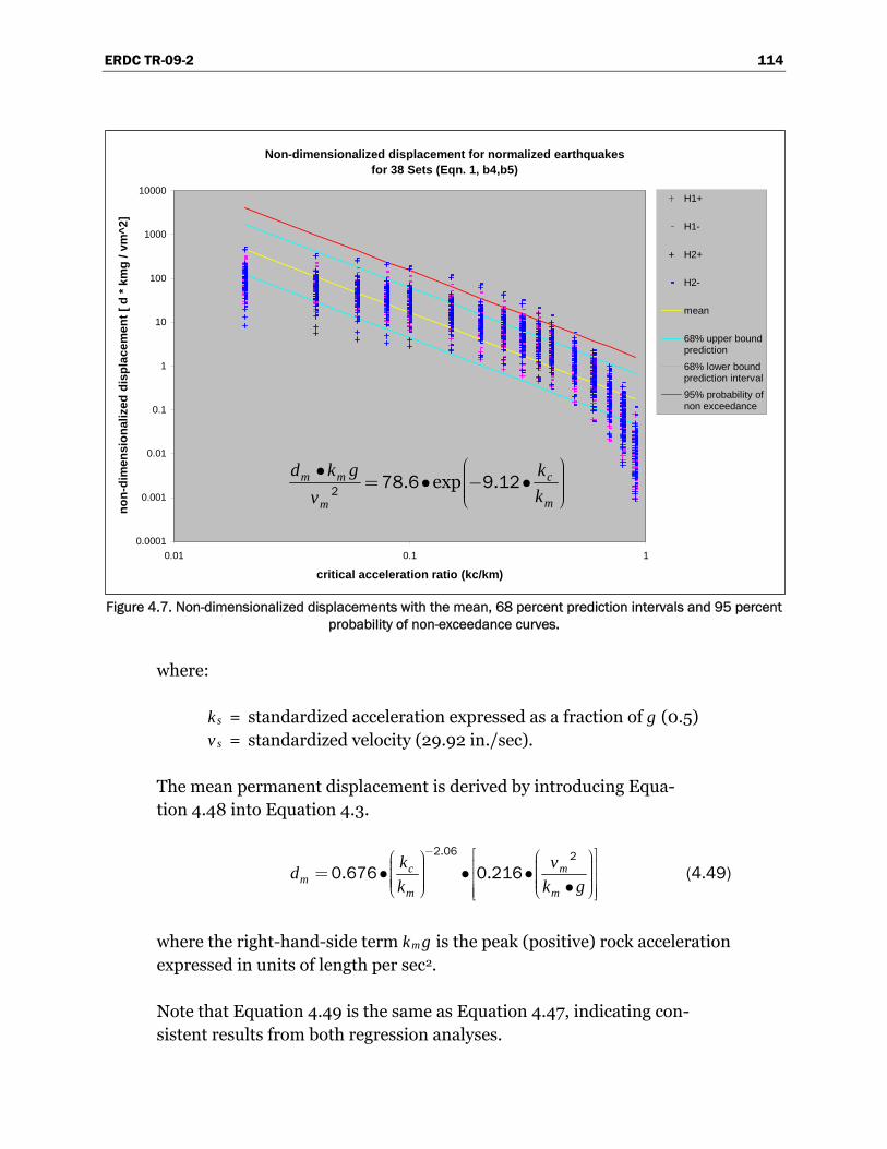
ERDC TR-09-2 114

Non-dimensionalized displacement for normalized earthquakes for 38 Sets (Eqn. 1, b4,b5)

0.0001

0.001

0.01

0.1

1

10

100

1000

10000

0.01 0.1 1


non-

dim

ensi

onal

ized

dis

plac

emen

t [ d

* km

g / v

m^2

]

H1+

H1-

H2+

H2-

mean




. exp .m m c

mm

d k g k

kv

⎛ ⎞• ⎟⎜ ⎟= • − •⎜ ⎟⎜ ⎟⎜⎝ ⎠2 78 6 9 12


where:



.

. .cm

m m

k vd

km

k g

− ⎡ ⎤⎛ ⎞⎛ ⎞ ⎟⎟ ⎜⎜ ⎢ ⎥⎟⎟= • • •⎜⎜ ⎟⎟ ⎢ ⎥⎜⎜ ⎟⎟⎜ ⎜ •⎝ ⎠ ⎝ ⎠⎢ ⎥⎣ ⎦

2 06 2

0 676 0 216 (4.49)



ERDC TR-09-2 115



.

.m m c

mm

d k g kkv

−⎛ ⎞• ⎟⎜ ⎟= • •⎜ ⎟⎜ ⎟⎜⎝ ⎠

2 06

2 0 146 2 60. (4.50)



.

. cs

m

kd

k

−⎛ ⎞⎟⎜ ⎟= • •⎜ ⎟⎜ ⎟⎜⎝ ⎠

2 06

0 676 2 60. (4.51)


.

. . .cm

m m

kd

k kmv

g

− ⎡ ⎤⎛ ⎞⎛ ⎞ ⎟⎟ ⎜⎜ ⎢ ⎥⎟⎟= • • • •⎜⎜ ⎟⎟ ⎢ ⎥⎜⎜ ⎟⎟⎜ ⎜ •⎝ ⎠ ⎝ ⎠⎢ ⎥⎣ ⎦

2 06 2

0 676 2 60 0 216 (4.52)





.

.m m c

mm

d k g kkv

−⎛ ⎞• ⎟⎜ ⎟= • •⎜ ⎟⎜ ⎟⎜⎝ ⎠

2 06

2 0 146 1 79. (4.53a)

ERDC TR-09-2 116

.

.m m c

mm

d k g kkv

−⎛ ⎞• ⎟⎜ ⎟= • •⎜ ⎟⎜ ⎟⎜⎝ ⎠

2 06

2 0 146 0 560. (4.53b)



.

. cs

m

kd

k

−⎛ ⎞⎟⎜ ⎟= •⎜ ⎟⎜ ⎟⎜⎝ ⎠

2 06

0 676 1 79. (4.54a)

.

. cs

m

kd

k

−⎛ ⎞⎟⎜ ⎟= • •⎜ ⎟⎜ ⎟⎜⎝ ⎠

2 06

0 676 0 560. (4.54b)


.

. . .c mm

m m

kd

k kv

g

− ⎡ ⎤⎛ ⎞⎛ ⎞ ⎟⎟ ⎜⎜ ⎢ ⎥⎟⎟= • • • •⎜⎜ ⎟⎟ ⎢ ⎥⎜⎜ ⎟⎟⎜ ⎜ •⎝ ⎠ ⎝ ⎠⎢ ⎥⎣ ⎦

2 06 2

0 676 1 79 0 216 (4.55a)

.

. . .c mm

m m

k vd

k k g

− ⎡ ⎤⎛ ⎞⎛ ⎞ ⎟⎟ ⎜⎜ ⎢ ⎥⎟⎟= • • • •⎜⎜ ⎟⎟ ⎢ ⎥⎜⎜ ⎟⎟⎜ ⎜ •⎝ ⎠ ⎝ ⎠⎢ ⎥⎣ ⎦

2 06 2

0 676 0 560 0 216 (4.55b)



4.3.4 Comparison of regression results of all three forms of the simplified non-dimensionalized displacement relationships

The three forms of regression analysis (discussed in Sections 4.3.1, 4.3.2, and 4.3.3), namely, the three-term regression analysis (eqn3 in Figure 4.8), the two-term, linear in Natural Logarithm Transformation (eqn2 in Fig-ure 4.8) and the two-term, linear in common logarithm transformation (eqn1 in Figure 4.8) will have their results compared and evaluated.

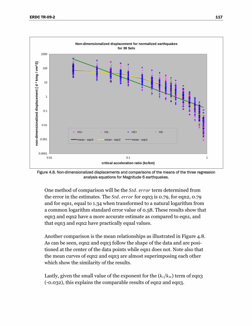
ERDC TR-09-2 117

Non-dimensionalized displacement for normalized earthquakes for 38 Sets

0.0001

0.001

0.01

0.1

1

10

100

1000

0.01 0.1 1


non-

dim

ensi

onal

ized

dis

plac

emen

t [ d

* km

g / v

m^2

]

H1+ H1- H2+ H2-





Another comparison is the mean relationships as illustrated in Figure 4.8. As can be seen, eqn2 and eqn3 follow the shape of the data and are posi-tioned at the center of the data points while eqn1 does not. Note also that the mean curves of eqn2 and eqn3 are almost superimposing each other which show the similarity of the results.


ERDC TR-09-2 118

4.4 Regression results of earthquakes covering the Moment Magnitude (Mw) range from 4.9 – 6.1 (Magnitude 5)

This subsequent section will discuss the results from regression analyses of the non-dimensionalized displacement relationships described by Equations 3.20, 3.39, and 3.58 previously derived in chapter three. The values for the coefficients summarized by the above mentioned equations and the standard error terms as well as the probabilistic measures of Equation Forms One, Two and Three, as documented in Table 4.8, will be discussed in Sections 4.4.1, 4.4.2, and 4.4.3. These regression analyses were performed for baseline corrected acceleration time histories recorded on rock with Mw range of 4.9 to 6.1 and an average Mw of 5.6.



β1 56.980 51.077

β2 -8.579 -8.436

β3 -0.039

β4 -0.153

β5 -1.940

Std. Error 1.242 0.738 0.738


The standard error term (Std. error) for this regression analysis was determined to be 0.74 for both the non-dimensionalized displacement as well as the standardized displacement for earthquakes of Magnitude 5. This non-dimensionalized three-term displacement equation is identified as Equation Form Three with the coefficients and Std. error terms summarized in column four of Table 4.8.



ERDC TR-09-2 119

.

. exp .m m c c

m mm

d k g k kk kv

−⎛ ⎞ ⎛ ⎞• ⎟ ⎟⎜ ⎜⎟ ⎟= • − • •⎜ ⎜⎟ ⎟⎜ ⎜⎟ ⎟⎜ ⎜⎝ ⎠ ⎝ ⎠

0 039

2 51 1 8 44 (4.56)

where:





Non-dimensionalized displacement for normalized earthquakes for 61 Sets(Eqn. 3, b1, b2, b3)

0.0001

0.001

0.01

0.1

1

10

100

1000

0.01 0.1 1


non-

dim

ensi

onal

ized

dis

plac

emen

t [ d

* km

g / v

m^2

]

H1+

H1-

H2+

H2-

mean


68% lower boundprediction interval95% probability ofnon exceedance

.

. exp .m m c c

m mm

d k g k kk kv

−⎛ ⎞ ⎛ ⎞• ⎟ ⎟⎜ ⎜⎟ ⎟= • − • •⎜ ⎜⎟ ⎟⎜ ⎜⎟ ⎟⎜ ⎜⎝ ⎠ ⎝ ⎠

0 039

2 51 1 8 44


ERDC TR-09-2 120

By a second independent regression analysis, the mean standardized maximum displacement (ds) in units of inches was derived for the standardized velocity, vs = 29.92 in./sec (0.76 m/sec) and the standardized acceleration ks = 0.5 g (193.04 in./sec2 : 4.90 m/sec2)

.

. exp . c cs

m m

k kd

k k

−⎛ ⎞ ⎛ ⎞⎟ ⎟⎜ ⎜⎟ ⎟= • − • •⎜ ⎜⎟ ⎟⎜ ⎜⎟ ⎟⎜ ⎜⎝ ⎠ ⎝ ⎠

0 039

236 9 8 44 (4.57)


s mm s

ms

k vd d

kv

⎡ ⎤⎛ ⎞ ⎛ ⎞⎟⎜ ⎜ ⎟⎢ ⎥⎟= • •⎜ ⎜⎟ ⎟⎟⎢ ⎥⎜ ⎜⎟⎜ ⎜⎝ ⎠ ⎝ ⎠⎟⎢ ⎥⎣ ⎦

2

2 (bis 4.3)

where:



.

. exp . .c c mm

m m m

k k vd

k k k g

− ⎡ ⎤⎛ ⎞⎛ ⎞ ⎛ ⎞ ⎟⎟ ⎟ ⎜⎜ ⎜ ⎢ ⎥⎟⎟ ⎟= • − • • • •⎜⎜ ⎜ ⎟⎟ ⎟ ⎢ ⎥⎜⎜ ⎜ ⎟⎟ ⎟⎜ ⎜ ⎜ •⎝ ⎠ ⎝ ⎠ ⎝ ⎠⎢ ⎥⎣ ⎦

0 039 2

236 9 8 44 0 216 (4.58)





ERDC TR-09-2 121

.

. exp . .m m c c

m mm

d k g k kk kv

−⎛ ⎞ ⎛ ⎞• ⎟ ⎟⎜ ⎜⎟ ⎟= • − • • •⎜ ⎜⎟ ⎟⎜ ⎜⎟ ⎟⎜ ⎜⎝ ⎠ ⎝ ⎠

0 039

2 51 1 8 44 3 39 (4.59)



.

. exp . c cs

m m

k kd

k k

−⎛ ⎞ ⎛ ⎞⎟ ⎟⎜ ⎜⎟ ⎟= • − • • •⎜ ⎜⎟ ⎟⎜ ⎜⎟ ⎟⎜ ⎜⎝ ⎠ ⎝ ⎠

0 039

236 9 8 44 3 39. (4.60)


.

. exp . . .c c mm

m m m

k k vd

k k k g

− ⎡ ⎤⎛ ⎞⎛ ⎞ ⎛ ⎞ ⎟⎟ ⎟ ⎜⎜ ⎜ ⎢ ⎥⎟⎟ ⎟= • − • • • • •⎜⎜ ⎜ ⎟⎟ ⎟ ⎢ ⎥⎜⎜ ⎜ ⎟⎟ ⎟⎜ ⎜ ⎜ •⎝ ⎠ ⎝ ⎠ ⎝ ⎠⎢ ⎥⎣ ⎦

0 039 2

236 9 8 44 3 39 0 216 (4.61)





.

. exp . .m m c c

m mm

d k g k kk kv

−⎛ ⎞ ⎛ ⎞• ⎟ ⎟⎜ ⎜⎟ ⎟= • − • • •⎜ ⎜⎟ ⎟⎜ ⎜⎟ ⎟⎜ ⎜⎝ ⎠ ⎝ ⎠

0 039

2 51 1 8 44 2 10 (4.62a)

.

. exp . .m m c c

m mm

d k g k kk kv

−⎛ ⎞ ⎛ ⎞• ⎟ ⎟⎜ ⎜⎟ ⎟= • − • • •⎜ ⎜⎟ ⎟⎜ ⎜⎟ ⎟⎜ ⎜⎝ ⎠ ⎝ ⎠

0 039

2 51 1 8 44 0 477 (4.62b)


ERDC TR-09-2 122


.

. exp . c cs

m m

k kd

k k

−⎛ ⎞ ⎛ ⎞⎟ ⎟⎜ ⎜⎟ ⎟= • − • • •⎜ ⎜⎟ ⎟⎜ ⎜⎟ ⎟⎜ ⎜⎝ ⎠ ⎝ ⎠

0 039

236 9 8 44 2 10. (4.63a)

.

. exp . .c cs

m m

k kd

k k

−⎛ ⎞ ⎛ ⎞⎟ ⎟⎜ ⎜⎟ ⎟= • − • • •⎜ ⎜⎟ ⎟⎜ ⎜⎟ ⎟⎜ ⎜⎝ ⎠ ⎝ ⎠

0 039

236 9 8 44 0 477 (4.63b)


.

. exp . . .c c mm

m m m

k k vd

k k k g

− ⎡ ⎤⎛ ⎞⎛ ⎞ ⎛ ⎞ ⎟⎟ ⎟ ⎜⎜ ⎜ ⎢ ⎥⎟⎟ ⎟= • − • • • • •⎜⎜ ⎜ ⎟⎟ ⎟ ⎢ ⎥⎜⎜ ⎜ ⎟⎟ ⎟⎜ ⎜ ⎜ •⎝ ⎠ ⎝ ⎠ ⎝ ⎠⎢ ⎥⎣ ⎦

0 039 2

236 9 8 44 2 10 0 216 (4.64a)

.

. exp . . .c c mm

m m m

k k vd

k k k g

− ⎡ ⎤⎛ ⎞⎛ ⎞ ⎛ ⎞ ⎟⎟ ⎟ ⎜⎜ ⎜ ⎢ ⎥⎟⎟ ⎟= • − • • • • •⎜⎜ ⎜ ⎟⎟ ⎟ ⎢ ⎥⎜⎜ ⎜ ⎟⎟ ⎟⎜ ⎜ ⎜ •⎝ ⎠ ⎝ ⎠ ⎝ ⎠⎢ ⎥⎣ ⎦

0 039 2

236 9 8 44 0 477 0 216 (4.64b)

where the right-hand-side term kmg is the peak (positive) rock acceleration expressed in units of length per sec2



The standard error term (Std. error) for this regression analysis was deter-mined to be 0.74 for both the non-dimensionalized displacement as well as the standardized displacement for earthquakes of Magnitude 5. This non-dimensionalized two-term displacement equation is identified as Equation Form Two with the coefficients and Std. error terms summarized in column three of Table 4.8.

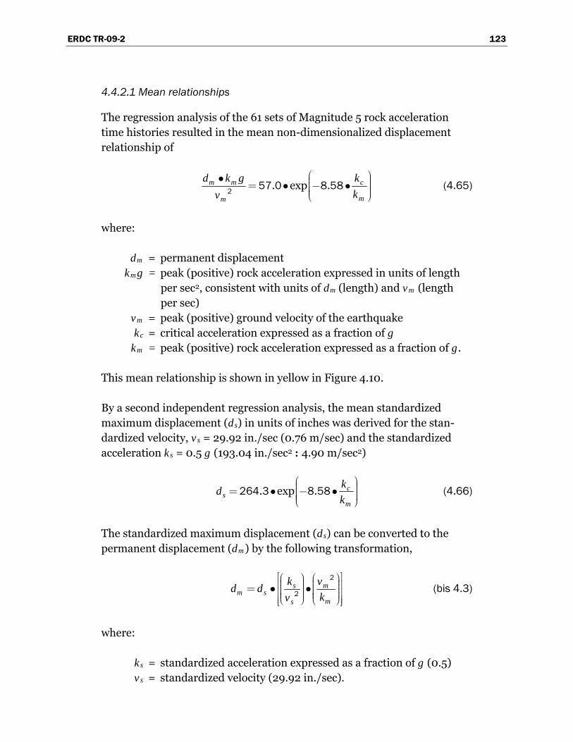
ERDC TR-09-2 123



. exp .m m c

mm

d k g k

kv

⎛ ⎞• ⎟⎜ ⎟= • − •⎜ ⎟⎜ ⎟⎜⎝ ⎠2 57 0 8 58 (4.65)

where:






. exp . cs

m

kd

k

⎛ ⎞⎟⎜ ⎟= • − •⎜ ⎟⎜ ⎟⎜⎝ ⎠264 3 8 58 (4.66)


s mm s

ms

k vd d

kv

⎡ ⎤⎛ ⎞ ⎛ ⎞⎟⎜ ⎜ ⎟⎢ ⎥⎟= • •⎜ ⎜⎟ ⎟⎟⎢ ⎥⎜ ⎜⎟⎜ ⎜⎝ ⎠ ⎝ ⎠⎟⎢ ⎥⎣ ⎦

2

2 (bis 4.3)

where:


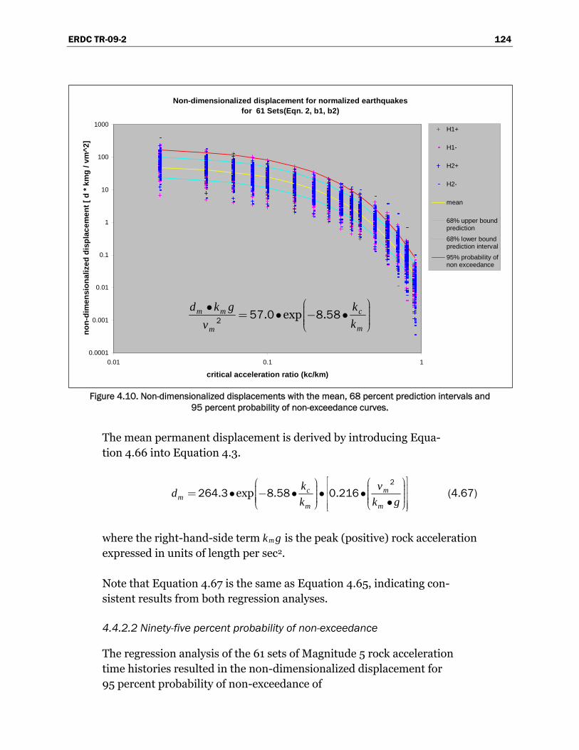
ERDC TR-09-2 124

Non-dimensionalized displacement for normalized earthquakes for 61 Sets(Eqn. 2, b1, b2)

0.0001

0.001

0.01

0.1

1

10

100

1000

0.01 0.1 1


non-

dim

ensi

onal

ized

dis

plac

emen

t [ d

* km

g / v

m^2

]

H1+

H1-

H2+

H2-

mean




. exp .m m c

mm

d k g k

kv

⎛ ⎞• ⎟⎜ ⎟= • − •⎜ ⎟⎜ ⎟⎜⎝ ⎠2 57 0 8 58



. exp . .cm

m m

k vd

k km

g

⎡ ⎤⎛ ⎞⎛ ⎞ ⎟⎟ ⎜⎜ ⎢ ⎥⎟⎟= • − • • •⎜⎜ ⎟⎟ ⎢ ⎥⎜⎜ ⎟⎟⎜ ⎜ •⎝ ⎠ ⎝ ⎠⎢ ⎥⎣ ⎦

2

264 3 8 58 0 216 (4.67)





ERDC TR-09-2 125

. exp .m m c

mm

d k g k

kv

⎛ ⎞• ⎟⎜ ⎟= • − • •⎜ ⎟⎜ ⎟⎜⎝ ⎠2 57 0 8 58 3 39. (4.68)



. exp . cs

m

kd

k

⎛ ⎞⎟⎜ ⎟= • − • •⎜ ⎟⎜ ⎟⎜⎝ ⎠264 3 8 58 3 39. (4.69)


. exp . . .c mm

m m

k vd

k k g

⎡ ⎤⎛ ⎞⎛ ⎞ ⎟⎟ ⎜⎜ ⎢ ⎥⎟⎟= • − • • • •⎜⎜ ⎟⎟ ⎢ ⎥⎜⎜ ⎟⎟⎜ ⎜ •⎝ ⎠ ⎝ ⎠⎢ ⎥⎣ ⎦

2

264 3 8 58 3 39 0 216 (4.70)





. exp .m m c

mm

d k g k

kv

⎛ ⎞• ⎟⎜ ⎟= • − • •⎜ ⎟⎜ ⎟⎜⎝ ⎠2 57 0 8 58 2 10. (4.71a)

. exp . .m m c

mm

d k g k

kv

⎛ ⎞• ⎟⎜ ⎟= • − • •⎜ ⎟⎜ ⎟⎜⎝ ⎠2 57 0 8 58 0 477 (4.71b)


ERDC TR-09-2 126


. exp . cs

m

kd

k

⎛ ⎞⎟⎜ ⎟= • − • •⎜ ⎟⎜ ⎟⎜⎝ ⎠264 3 8 58 2 10. (4.72a)

. exp . .cs

m

kd

k

⎛ ⎞⎟⎜ ⎟= • − • •⎜ ⎟⎜ ⎟⎜⎝ ⎠264 3 8 58 0 477 (4.72b)


. exp . . .c mm

m m

k vd

k k g

⎡ ⎤⎛ ⎞⎛ ⎞ ⎟⎟ ⎜⎜ ⎢ ⎥⎟⎟= • − • • • •⎜⎜ ⎟⎟ ⎢ ⎥⎜⎜ ⎟⎟⎜ ⎜ •⎝ ⎠ ⎝ ⎠⎢ ⎥⎣ ⎦

2

264 3 8 58 2 10 0 216 (4.73a)

. exp . . .c mm

m m

k vd

k k g

⎡ ⎤⎛ ⎞⎛ ⎞ ⎟⎟ ⎜⎜ ⎢ ⎥⎟⎟= • − • • • •⎜⎜ ⎟⎟ ⎢ ⎥⎜⎜ ⎟⎟⎜ ⎜ •⎝ ⎠ ⎝ ⎠⎢ ⎥⎣ ⎦

2

264 3 8 58 0 477 0 216 (4.73b)





ERDC TR-09-2 127



.

.m m c

mm

d k g kkv

−⎛ ⎞• ⎟⎜ ⎟= •⎜ ⎟⎜ ⎟⎜⎝ ⎠

1 94

2 0 153 (4.74)

where:






.

. cs

m

kd

k

−⎛ ⎞⎟⎜ ⎟= •⎜ ⎟⎜ ⎟⎜⎝ ⎠

1 94

0 71 (4.75)


s mm s

ms

k vd d

kv

⎡ ⎤⎛ ⎞ ⎛ ⎞⎟⎜ ⎜ ⎟⎢ ⎥⎟= • •⎜ ⎜⎟ ⎟⎟⎢ ⎥⎜ ⎜⎟⎜ ⎜⎝ ⎠ ⎝ ⎠⎟⎢ ⎥⎣ ⎦

2

2 (bis 4.3)

where:


ERDC TR-09-2 128

Non-dimensionalized displacement for normalized earthquakes for 61 Sets(Eqn. 1, b4,b5)

0.0001

0.001

0.01

0.1

1

10

100

1000

10000

0.01 0.1 1


non-

dim

ensi

onal

ized

dis

plac

emen

t [ d

* km

g / v

m^2

]

H1+

H1-

H2+

H2-

mean




.

.m m c

mm

d k g kkv

−⎛ ⎞• ⎟⎜ ⎟= •⎜ ⎟⎜ ⎟⎜⎝ ⎠

1 94

2 0 153



.

. .cm

m m

k vd

km

k g

− ⎡ ⎤⎛ ⎞⎛ ⎞ ⎟⎟ ⎜⎜ ⎢ ⎥⎟⎟= • • •⎜⎜ ⎟⎟ ⎢ ⎥⎜⎜ ⎟⎟⎜ ⎜ •⎝ ⎠ ⎝ ⎠⎢ ⎥⎣ ⎦

1 94 2

0 71 0 216 (4.76)





ERDC TR-09-2 129

.

.m m c

mm

d k g kkv

−⎛ ⎞• ⎟⎜ ⎟= • •⎜ ⎟⎜ ⎟⎜⎝ ⎠

1 94

2 0 153 2 44. (4.77)



.

. cs

m

kd

k

−⎛ ⎞⎟⎜ ⎟= • •⎜ ⎟⎜ ⎟⎜⎝ ⎠

1 94

0 71 2 44. (4.78)


.

. . .cm

m m

kd

k kmv

g

− ⎡ ⎤⎛ ⎞⎛ ⎞ ⎟⎟ ⎜⎜ ⎢ ⎥⎟⎟= • • • •⎜⎜ ⎟⎟ ⎢ ⎥⎜⎜ ⎟⎟⎜ ⎜ •⎝ ⎠ ⎝ ⎠⎢ ⎥⎣ ⎦

1 94 2

0 71 2 44 0 216 (4.79)





.

.m m c

mm

d k g kkv

−⎛ ⎞• ⎟⎜ ⎟= • •⎜ ⎟⎜ ⎟⎜⎝ ⎠

1 94

2 0 153 1 72. (4.80a)

.

.m m c

mm

d k g kkv

−⎛ ⎞• ⎟⎜ ⎟= • •⎜ ⎟⎜ ⎟⎜⎝ ⎠

1 94

2 0 153 0 583. (4.80b)


ERDC TR-09-2 130


.

. cs

m

kd

k

−⎛ ⎞⎟⎜ ⎟= • •⎜ ⎟⎜ ⎟⎜⎝ ⎠

1 94

0 71 1 72. (4.81a)

.

. cs

m

kd

k

−⎛ ⎞⎟⎜ ⎟= • •⎜ ⎟⎜ ⎟⎜⎝ ⎠

1 94

0 71 0 583. (4.81b)


.

. . .cm

m m

kd

k kmv

g

− ⎡ ⎤⎛ ⎞⎛ ⎞ ⎟⎟ ⎜⎜ ⎢ ⎥⎟⎟= • • • •⎜⎜ ⎟⎟ ⎢ ⎥⎜⎜ ⎟⎟⎜ ⎜ •⎝ ⎠ ⎝ ⎠⎢ ⎥⎣ ⎦

1 94 2

0 71 1 72 0 216 (4.82a)

.

. . .c mm

m m

kd

k kv

g

− ⎡ ⎤⎛ ⎞⎛ ⎞ ⎟⎟ ⎜⎜ ⎢ ⎥⎟⎟= • • • •⎜⎜ ⎟⎟ ⎢ ⎥⎜⎜ ⎟⎟⎜ ⎜ •⎝ ⎠ ⎝ ⎠⎢ ⎥⎣ ⎦

1 94 2

0 71 0 583 0 216 (4.82b)



4.4.4 Comparison of regression results of all three forms of the simplified non-dimensionalized displacement relationships.

The three forms of regression analysis (discussed in Sections 4.4.1, 4.4.2, and 4.4.3), namely, the three-term regression analysis (identified as eqn3 in Figure 4.12), the two-term, linear in Natural Logarithm Transformation (eqn2 in Figure 4.12) and the two-term, linear in common logarithm trans-formation (eqn1 in Figure 4.12) will have their results compared and evaluated.

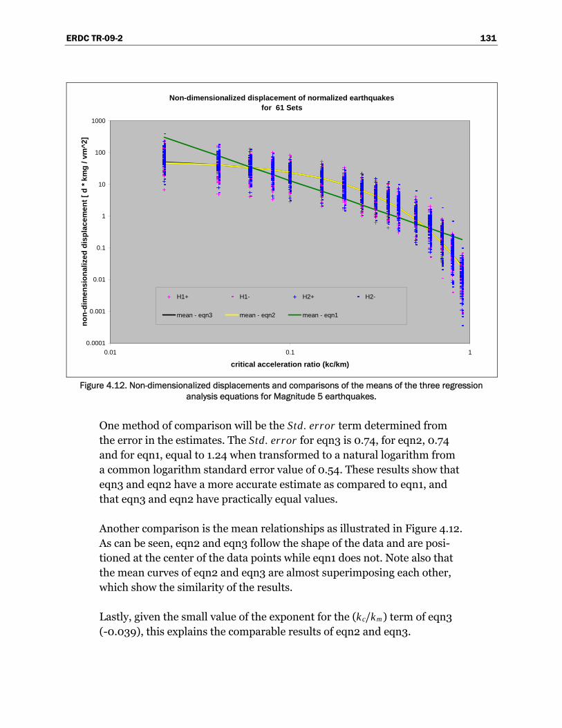
ERDC TR-09-2 131

Non-dimensionalized displacement of normalized earthquakes for 61 Sets

0.0001

0.001

0.01

0.1

1

10

100

1000

0.01 0.1 1


non-

dim

ensi

onal

ized

dis

plac

emen

t [ d

* km

g / v

m^2

]

H1+ H1- H2+ H2-





Another comparison is the mean relationships as illustrated in Figure 4.12. As can be seen, eqn2 and eqn3 follow the shape of the data and are posi-tioned at the center of the data points while eqn1 does not. Note also that the mean curves of eqn2 and eqn3 are almost superimposing each other, which show the similarity of the results.


ERDC TR-09-2 132

4.5 Special regression results of Equation Form Two of non-dimensionalized displacement relationships without differentiation of Moment Magnitude

This subsequent section will discuss the results from regression analyses of the non-dimensionalized displace-ment relationships described by Equation 3.39, previously derived in Chapter 3. The values for the coeffi-cients summarized by the above-mentioned equation and the standard error terms as well as the probabil-istic measures of Equation Form Two are documented in Table 4.9 and will be discussed in Sections 4.5.1, 4.5.2, and 4.5.3. The regression analysis was performed for baseline corrected acceleration time histories recorded on rock with Mw range of 4.9 to 8.1.

Table 4.9. Values for the regression Equation Form Two constants without differentiation of Mw.

Coefficients and Std. Error Equation Form Two

β1 64.439

β2 -8.862

β3

β4

β5

Std. Error 0.800

The standard error term (Std. error) for this regression analysis was deter-mined to be 0.80 for both the non-dimensionalized displacement as well as the standardized displacement. This non-dimensionalized two-term displacement equation is identified as Equation Form Two with the coeffi-cients and Std. error terms summarized in column two of Table 4.9.

4.5.1. Mean relationships

The regression analysis of the 122 sets of Magnitude 5 – 7 rock accelera-tion time histories resulted in the mean non-dimensionalized displace-ment relationship of

. exp .m m c

mm

d k g k

kv

⎛ ⎞• ⎟⎜ ⎟= • − •⎜ ⎟⎜ ⎟⎜⎝ ⎠2 65 44 8 86 (4.83)

where:



vm = peak (positive) ground velocity of the earthquake

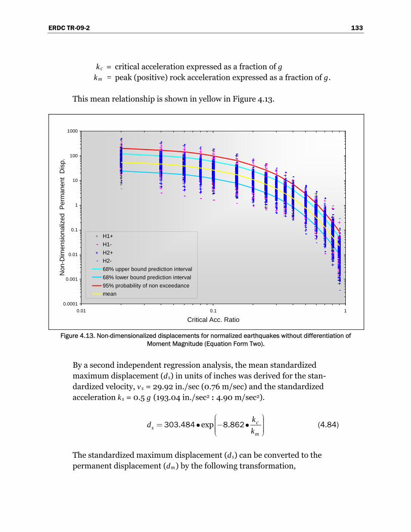
ERDC TR-09-2 133

kc = critical acceleration expressed as a fraction of g km = peak (positive) rock acceleration expressed as a fraction of g.


0.0001

0.001

0.01

0.1

1

10

100

1000

0.01 0.1 1

Critical Acc. Ratio

Non

-Dim

ensi

onal

ized

Per

man

ent

Dis

p.

H1+H1-H2+H2-68% upper bound prediction interval68% lower bound prediction interval95% probability of non exceedancemean

Figure 4.13. Non-dimensionalized displacements for normalized earthquakes without differentiation of

Moment Magnitude (Equation Form Two).

By a second independent regression analysis, the mean standardized maximum displacement (ds) in units of inches was derived for the stan-dardized velocity, vs = 29.92 in./sec (0.76 m/sec) and the standardized acceleration ks = 0.5 g (193.04 in./sec2 : 4.90 m/sec2).

. exp . cs

m

kd

k

⎛ ⎞⎟⎜ ⎟= • − •⎜ ⎟⎜ ⎟⎜⎝ ⎠303 484 8 862 (4.84)


ERDC TR-09-2 134

s mm s

ms

k vd d

kv

⎡ ⎤⎛ ⎞ ⎛ ⎞⎟⎜ ⎜ ⎟⎢ ⎥⎟= • •⎜ ⎜⎟ ⎟⎟⎢ ⎥⎜ ⎜⎟⎜ ⎜⎝ ⎠ ⎝ ⎠⎟⎢ ⎥⎣ ⎦

2

2 (bis 4.3)

where:



. exp . .cm

m m

kd

k kmv

g

⎡ ⎤⎛ ⎞⎛ ⎞ ⎟⎟ ⎜⎜ ⎢ ⎥⎟⎟= • − • • •⎜⎜ ⎟⎟ ⎢ ⎥⎜⎜ ⎟⎟⎜ ⎜ •⎝ ⎠ ⎝ ⎠⎢ ⎥⎣ ⎦

2

303 484 8 862 0 216 (4.86)


Note that Equation 4.83 is the approximately the same as Equation 4.86, indicating consistent results from both regression analyses.

4.5.2 Ninety-five percent probability of non-exceedance

The regression analysis of the 122 sets of Mw 5 to 7 rock acceleration time histories resulted in the non-dimensionalized displacement for 95 percent probability of non-exceedance of

. exp .m m c

mm

d k g k

kv

⎛ ⎞• ⎟⎜ ⎟= • − • •⎜ ⎟⎜ ⎟⎜⎝ ⎠2 65 44 8 86 3 75. (4.87)



. exp . cs

m

kd

k

⎛ ⎞⎟⎜ ⎟= • − • •⎜ ⎟⎜ ⎟⎜⎝ ⎠303 484 8 86 3 75. (4.88)

ERDC TR-09-2 135


. exp . . .c mm

m m

k vd

k k g

⎡ ⎤⎛ ⎞⎛ ⎞ ⎟⎟ ⎜⎜ ⎢ ⎥⎟⎟= • − • • • •⎜⎜ ⎟⎟ ⎢ ⎥⎜⎜ ⎟⎟⎜ ⎜ •⎝ ⎠ ⎝ ⎠⎢ ⎥⎣ ⎦

2

303 484 8 86 3 75 0 216 (4.89)


Note that Equation 4.89 is the approximately the same as Equation 4.87, indicating consistent results from both regression analyses.

4.5.3 Sixty-eight percent prediction intervals

The regression analysis of the 122 sets of Magnitude 5 - 7 rock acceleration time histories resulted in the non-dimensionalized displacement relation-ships for the 68 percent prediction intervals of

. exp .m m c

mm

d k g k

kv

⎛ ⎞• ⎟⎜ ⎟= • − • •⎜ ⎟⎜ ⎟⎜⎝ ⎠2 65 44 8 86 2 23. (4.90a)

. exp . .m m c

mm

d k g k

kv

⎛ ⎞• ⎟⎜ ⎟= • − • •⎜ ⎟⎜ ⎟⎜⎝ ⎠2 65 44 8 86 0 449 (4.90b)



. exp . cs

m

kd

k

⎛ ⎞⎟⎜ ⎟= • − • •⎜ ⎟⎜ ⎟⎜⎝ ⎠303 484 8 86 2 23. (4.91a)

. exp . .cs

m

kd

k

⎛ ⎞⎟⎜ ⎟= • − • •⎜ ⎟⎜ ⎟⎜⎝ ⎠303 484 8 86 0 449 (4.91b)


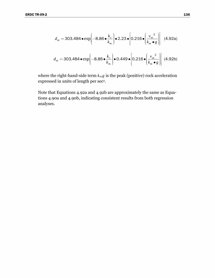
ERDC TR-09-2 136

. exp . . .c mm

m m

k vd

k k g

⎡ ⎤⎛ ⎞⎛ ⎞ ⎟⎟ ⎜⎜ ⎢ ⎥⎟⎟= • − • • • •⎜⎜ ⎟⎟ ⎢ ⎥⎜⎜ ⎟⎟⎜ ⎜ •⎝ ⎠ ⎝ ⎠⎢ ⎥⎣ ⎦

2

303 484 8 86 2 23 0 216 (4.92a)

. exp . . .c mm

m m

k vd

k k g

⎡ ⎤⎛ ⎞⎛ ⎞ ⎟⎟ ⎜⎜ ⎢ ⎥⎟⎟= • − • • • •⎜⎜ ⎟⎟ ⎢ ⎥⎜⎜ ⎟⎟⎜ ⎜ •⎝ ⎠ ⎝ ⎠⎢ ⎥⎣ ⎦

2

303 484 8 86 0 449 0 216 (4.92b)


Note that Equations 4.92a and 4.92b are approximately the same as Equa-tions 4.90a and 4.90b, indicating consistent results from both regression analyses.

ERDC TR-09-2 137

5 The Visual Modeler for Newmark – NewmarkVM

5.1 Introduction

This chapter provides guidance on the details of the Visual Modeler (NewmarkVM), the PC-based Graphical User Interface (GUI) to the pro-gram named Newmark. NewmarkVM gathers the necessary user specified information and provides a simple and expedient means of interpreting the results from a Newmark analysis (by executing Newmark, the FORTRAN engineering formulation discussed in Chapter 2). There will be discussions on how to perform and interpret the results of an analysis.

5.2 The Visual Modeling Environment

Newmark is a program that can perform a permanent sliding block dis-placement analysis given a baseline corrected rock site-specific accelera-tion time-history. Newmark can also conduct regression analyses for sets of rock founded acceleration time histories in order to develop up to three user selected forms of generalized equations of simplified permanent displacement relationships. The user has the option of performing one of two types of translational (i.e. sliding) analysis, either a single or deter-ministic analysis, or a multiple analysis that can include regression analyses.

At the onset of NewmarkVM, the user is automatically introduced to a graphical image representing the results obtained from a typical regres-sion analysis computed by Newmark. In this case, evaluation of 122 sets of (rock) acceleration time histories ranging from earthquake magnitudes of 5 thru 7 were used for the multiple analyses. This image is included in the Introduction tab and shown in Figure 5.1. Directly above this tab are two drop down menus. The first, entitled File, provides an easy and conven-ient way to open an existing file, create a new file or save existing data to a file. These files are user created and have an “.nmk” extension. Opening an existing file will immediately replenish the data within all tabs and thereby allow the user to quickly run an analysis from previous data input. The second drop down menu above the Introduction tab is labeled Analysis Type; here the user is given the option to select the scenario of either a single analysis or multiple analyses that may apply regression.

ERDC TR-09-2 138

Figure 5.1. The Introduction tab features the process of a multiple analysis.

5.2.1 Significant Tabs relevant to an analysis

With a single analysis, the input data to Newmark falls into three different groups and NewmarkVM displays these groups with the following tabs available for user input

• Earthquake Time-History Horizontal Component 1 data • Maximum Transmissible Acceleration values

ERDC TR-09-2 139

• Analysis of specified data

Input data for a multiple or regression analyses falls into six different groups and the NewmarkVM displays these groups as tabs and available for user input

• Multiple Horizontal Time-History Selections menu • Earthquake Time-History Horizontal Component 1 data • Earthquake Time-History Horizontal Component 2 data • Maximum Transmissible Acceleration values • Selection of Time Histories for analysis • Analysis of specified data

In order to perform multiple analyses, it is required that we consider only sets of acceleration time histories. A set is made up of two site-specific acceleration time-history files; each representing a horizontal component. If only one component is available for one or more sets of time histories, Newmark will acknowledge this fact and perform the analyses with the available time histories.

The following subsections of Section 5.2 are listed in the order as shown in the NewmarkVM tabs. Each subsection describes the function of each tab and identifies whether each tab relates to a single analysis, multiple analyses or both.

5.2.2 Multiple Horizontal Time-History Selections (Multiple Analyses only)

The function of this tab relates to the collection of sets of base-line corrected acceleration time histories as input and consists mainly of file handling. Figure 5.2 shows the many options necessary for the creation of a list of filenames relating to acceleration time histories for an analysis.

The user data entry within this tab will be described in a top-down manner. Data within this tab can be divided into subgroups and is described in the following two sections.

ERDC TR-09-2 140

Figure 5.2. The Multiple Horizontal Time-History Selections tab ready for user input.

5.2.2.1 Selection of Horizontal Earthquake Time-History Files

The Browse to Select Horizontal Earthquake Time-History File(s) allows the user to gather all relative acceleration time-history files necessary for computing multiple analyses. Once selected, a file manage-ment screen will appear for the user to choose all relevant files. The pull-down menu on the left of the screen (Figure 5.3) gives the path (i.e., drive and directory) to the location of the files. The large center box shows a list

ERDC TR-09-2 141

of files contained within the selected directory. The Copy Selected button at the right allows the selection of any or all files in the center box. If the user decides to start over or clear the list of files in the center box, the Clear List button on the upper right of the previous menu (Fig-ure 5.2) is an option used to remove the selected files. Finally, when the user is satisfied with all files, the OK button is accepted and the original screen of Section 5.2.2 will appear with the list of all selected files.

From the list of previously selected acceleration time-history files, the user can start matching the sets, i.e. the horizontal components of these earth-quake time histories need to belong to the same set. It is important to correctly pick the files that pertain to horizontal component 1 (group 1) and the files for horizontal component 2 (group 2). This is accomplished by the Assign File to frame or container located to the left in Figure 5.2 which contains 3 buttons. To select a set, use the following steps

1. Choose a file for group 1, by selecting the file listed in the center box and then pressing the Group#1 button

2. This file will appear in the File (H1) to Group #1: box within the New Time-History File Set frame

3. If file in step 2 is incorrect, select Clear H1 and start over with step 1 4. Choose a file for group 2, by selecting the file listed in the center box and

then pressing the Group#2 button 5. This group 2 file will appear in the File (H1) to Group #2: box within

the New Time-History File Set frame 6. If file in step 5 is incorrect, select Clear H2 and start over with step 4 for

selection of group 2 files. 7. Select the Add Set button located in the Assign File to frame to create

the set

Note: If there is no file pertaining to either group 1 or group 2, the user can take the default of N/A found within the New Time-History File Set frame.

After selecting the Add Set button, the new set will be added to a scroll-down list with a gray background, and each file will be located within its respective group number.

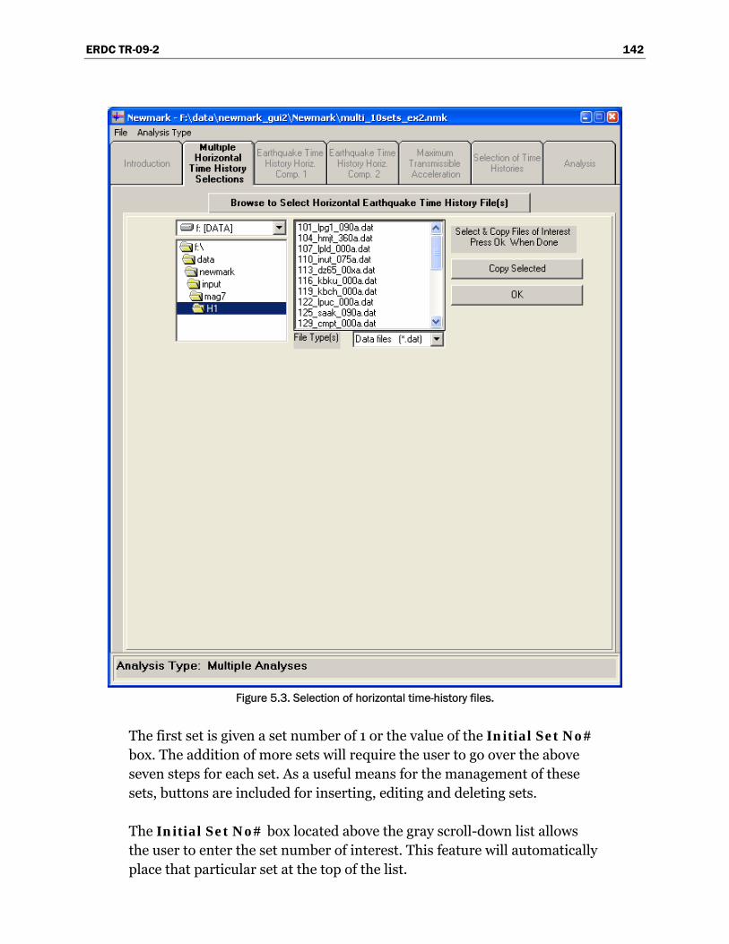
ERDC TR-09-2 142

Figure 5.3. Selection of horizontal time-history files.

The first set is given a set number of 1 or the value of the Initial Set No# box. The addition of more sets will require the user to go over the above seven steps for each set. As a useful means for the management of these sets, buttons are included for inserting, editing and deleting sets.

The Initial Set No# box located above the gray scroll-down list allows the user to enter the set number of interest. This feature will automatically place that particular set at the top of the list.

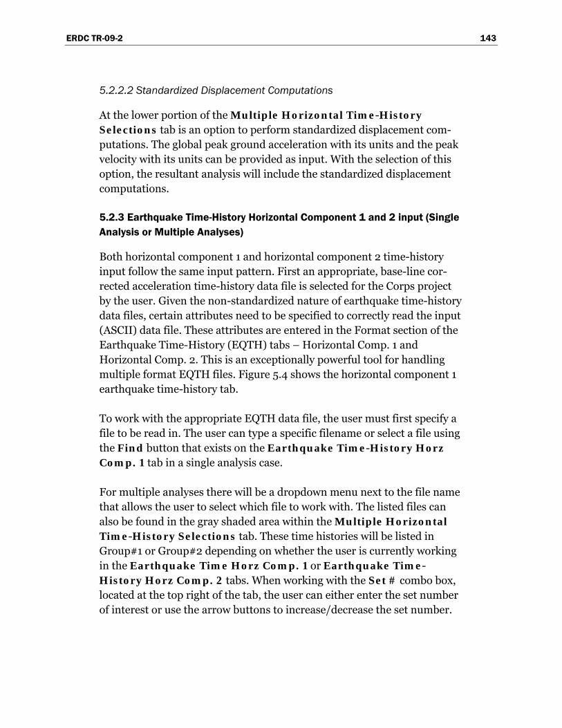
ERDC TR-09-2 143

5.2.2.2 Standardized Displacement Computations

At the lower portion of the Multiple Horizontal Time-History Selections tab is an option to perform standardized displacement com-putations. The global peak ground acceleration with its units and the peak velocity with its units can be provided as input. With the selection of this option, the resultant analysis will include the standardized displacement computations.

5.2.3 Earthquake Time-History Horizontal Component 1 and 2 input (Single Analysis or Multiple Analyses)

Both horizontal component 1 and horizontal component 2 time-history input follow the same input pattern. First an appropriate, base-line cor-rected acceleration time-history data file is selected for the Corps project by the user. Given the non-standardized nature of earthquake time-history data files, certain attributes need to be specified to correctly read the input (ASCII) data file. These attributes are entered in the Format section of the Earthquake Time-History (EQTH) tabs – Horizontal Comp. 1 and Horizontal Comp. 2. This is an exceptionally powerful tool for handling multiple format EQTH files. Figure 5.4 shows the horizontal component 1 earthquake time-history tab.

To work with the appropriate EQTH data file, the user must first specify a file to be read in. The user can type a specific filename or select a file using the Find button that exists on the Earthquake Time-History Horz Comp. 1 tab in a single analysis case.

For multiple analyses there will be a dropdown menu next to the file name that allows the user to select which file to work with. The listed files can also be found in the gray shaded area within the Multiple Horizontal Time-History Selections tab. These time histories will be listed in Group#1 or Group#2 depending on whether the user is currently working in the Earthquake Time Horz Comp. 1 or Earthquake Time-History Horz Comp. 2 tabs. When working with the Set # combo box, located at the top right of the tab, the user can either enter the set number of interest or use the arrow buttons to increase/decrease the set number.

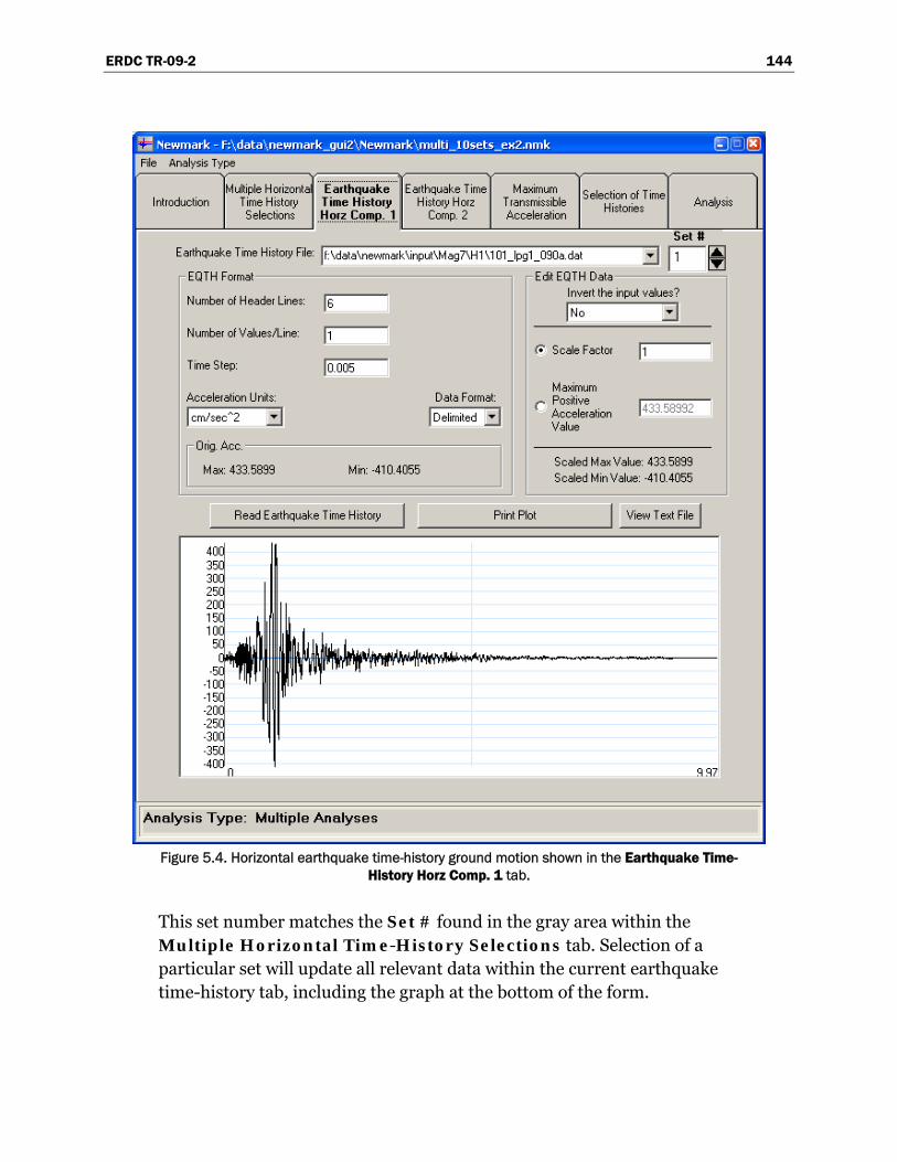
ERDC TR-09-2 144

Figure 5.4. Horizontal earthquake time-history ground motion shown in the Earthquake Time-

History Horz Comp. 1 tab.

This set number matches the Set # found in the gray area within the Multiple Horizontal Time-History Selections tab. Selection of a particular set will update all relevant data within the current earthquake time-history tab, including the graph at the bottom of the form.

ERDC TR-09-2 145

When a file has been selected, a format must be built. All specifications for reading a file are grouped in a frame labeled EQTH Format. To know what information to enter for reading the file, it will be beneficial to select the View Text File button and peruse the file to find each section of data.

The first block of data in each EQTH file is the number of header lines. Entering how many header lines there are allows the program to skip those lines. It is also important to know how many data samples are on each line. Entering the Number of Values/Line keeps the program from entering blank samples or ignoring samples. The value entered for Time Step should be the amount of time that occurs between samples, establishing the sampling frequency and the total time for the earthquake data.

Since Newmark works from the beginning of an earthquake, it is to be assumed that the first sample, time step 0, will have a value of 0.0 in what-ever units chosen. If the EQTH file does not have this zero point, it will be accounted for in the software.

There is a combo box that allows the user to specify the units that the data were recorded in. NOTE: The horizontal component 1 EQTH file uses the same units as the Horizontal component 2 EQTH file. There is no way to mix and match EQTH units.

There is a second combo box that shows several options for a data format. These formats are displayed as if they were in a FORTRAN FORMAT statement. These are especially important in areas where data text may run together. In the Data Format pull-down menu, the Delimited option is the space.

After an EQTH format has been built for a particular file, the user can read in the Earthquake Time-History. After the button is pressed, the actual values of the maximum and minimum values for that file are displayed in the Orig. Acc. sub-frame of the EQTH Format frame. A plot of the input data is also displayed at the bottom of the tab. The Edit EQTH Data frame will also be enabled.

The Edit EQTH Data frame is a tool that allows the user to scale the EQTH data to values more appropriate for modeling the problem at hand. There is a combo-box that allows the user to invert the user specified

ERDC TR-09-2 146

earthquake acceleration time-history values, which is valuable for deter-mining whether the direction of peak values influence the computed (permanent displacement) results.

There are also two possible ways of scaling the input data, either by setting an absolute scale value to multiply the samples by or by setting an absolute maximum value for the positive peak value and scaling the other samples to match. To choose the scale method, click the radio button beside that option. Then, type in the value desired.

When this is done, the inactive choice will be updated with the related value. Also, the scaled minimum and maximum values will be displayed, and the data plot at the bottom of the form will reflect the changes.

If the user desires a hardcopy of the scaled data in the same format as at the bottom of the tab, there is a button labeled Print Plot.

If the user would like to view the raw data in its original format, there is a button labeled View Text File.

5.2.4 Maximum Transmissible Acceleration input (Single Analysis or Multiple Analyses)

To perform a Newmark sliding block analysis, a maximum transmissible acceleration (as described in Section 1.1.3.2 of this report) has to be specified with this value of acceleration at the incipient of displacement resulting in a factor of safety less than of equal to 1.0. Figure 5.5 allows for user input for either a single analysis or multiple analyses.

In a single analysis, the user has the option of providing the maximum transmissible acceleration (kc) and its units or the ratio of kc and the peak acceleration (km) as user input.

For multiple analyses, the maximum transmissible acceleration is given as a fraction of the peak acceleration. Multiple kc /km values are necessary and the user has the option to add any values or accept the defaults (selected by the authors). The Multiple Analyses frame allows the user to modify the values by directly editing the existing 16 values; add additional values at the end of the list, delete and/or insert values.

ERDC TR-09-2 147

Figure 5.5. Maximum Transmissible Acceleration tab for multiple analyses data entry.

5.2.5 The Selection of Time Histories (Multiple Analyses)

This section summarizes a simple way of including all or excluding some files previously selected in the Multiple Horizontal Time-History Selections tab (Figure 5.6) for an analysis. The acceleration time histo-ries (i.e. the horizontal component 1 (H1) and horizontal component 2 (H2)) chosen will be used for user specified regression analyses and

ERDC TR-09-2 148

displayed after the completion of the execution of Newmark in the Analysis tab.

Figure 5.6. The Selection of Time Histories tab for data entry used for multiple analyses.

The first horizontal acceleration time-history set (i.e. H1 and H2) is dis-played within the View Earthquake Time-History Set frame and each labeled by File(H1): and File(H2): for the respective horizontal com-ponents. If either component was not available there would be an N/A placed instead of the name of the file. There is also a Choose Set to View

ERDC TR-09-2 149

entry/selection box with a default of 1 that allows the user to specify which set to list. This can be used to verify the files being used and is by no means a way of sorting the entire set of lists.

The earthquake time-history horizontal components H1 and H2 can fur-ther be evaluated by inverting the values of each horizontal component time-history. The reasoning for this is to determine whether the magni-tudes of H1 and/or H2 have an effect on the resultant (permanent dis-placement) analysis. Therefore, a separate time-history was created that is the inverse of the original. Thus, H1 is now H1(+), with an H1(-) as its inverse. The same logic is applied for H2.

About the center of this tab, there is the Global Select frame which allows the user an easy way to select any of the possible four horizontal components in a vertical sense (i.e. the selection of the H1(+) button will mark all the H1(+) buttons listed vertically in the sub-frame directly below). This feature also applies for the H1(-), H2(+), H2(-) buttons.

There is an All button, which accepts all files, and a None button, which clears out the files previous selected and un-marks all of the buttons.

The sub-frame located beneath the Global Select frame is used for selecting time histories on a set-by-set basis. For set 1, the user can mark or unmark any of the 4 buttons, i.e., H1(+), H1(-), H2(+), H2(-). There is an All button which accepts all files in this set and a None button which un-marks all the buttons of the current set. The sliding bar to the right allows the user to view which sets are marked or unmarked.

5.2.6 Analysis results (Single Analysis or Multiple Analyses)

The Figure 5.7 Analysis tab can be divided into three sections: Input Parameters, Run Newmark Analyzer and View Output. The Input Parameters section allows the user to select the regression analysis type and also set the output units from an execution of Newmark. The Run Newmark Analyzer section is a button that will execute the Newmark program. The View Output section contains options for viewing the many outputs of the Newmark Analysis, including the Regression Analysis subsection that allows the user to view the data and the statistic parameters derived from a multiple analysis.

ERDC TR-09-2 150

Figure 5.7. The Analysis tab used for all analyses.

In the Input Parameters frame of the Analysis tab, the user can select inputs from two combo boxes. The Regression Analysis Type combo box shows the option of no regression, performing regression analyses with three different forms of equations and the combinations of these equations.

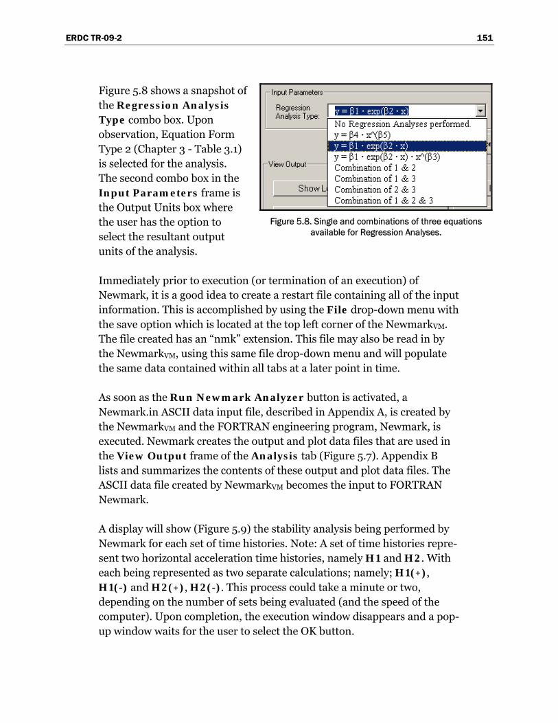
ERDC TR-09-2 151

Figure 5.8. Single and combinations of three equations available for Regression Analyses.

Figure 5.8 shows a snapshot of the Regression Analysis Type combo box. Upon observation, Equation Form Type 2 (Chapter 3 - Table 3.1) is selected for the analysis. The second combo box in the Input Parameters frame is the Output Units box where the user has the option to select the resultant output units of the analysis.

Immediately prior to execution (or termination of an execution) of Newmark, it is a good idea to create a restart file containing all of the input information. This is accomplished by using the File drop-down menu with the save option which is located at the top left corner of the NewmarkVM. The file created has an “nmk” extension. This file may also be read in by the NewmarkVM, using this same file drop-down menu and will populate the same data contained within all tabs at a later point in time.

As soon as the Run Newmark Analyzer button is activated, a Newmark.in ASCII data input file, described in Appendix A, is created by the NewmarkVM and the FORTRAN engineering program, Newmark, is executed. Newmark creates the output and plot data files that are used in the View Output frame of the Analysis tab (Figure 5.7). Appendix B lists and summarizes the contents of these output and plot data files. The ASCII data file created by NewmarkVM becomes the input to FORTRAN Newmark.

A display will show (Figure 5.9) the stability analysis being performed by Newmark for each set of time histories. Note: A set of time histories repre-sent two horizontal acceleration time histories, namely H1 and H2. With each being represented as two separate calculations; namely; H1(+), H1(-) and H2(+), H2(-). This process could take a minute or two, depending on the number of sets being evaluated (and the speed of the computer). Upon completion, the execution window disappears and a pop-up window waits for the user to select the OK button.

ERDC TR-09-2 152

Figure 5.9. Illustrative example of Newmark during execution.

The focus now returns to the Analysis Tab and the View Output section. The user has many options available for viewing and evaluating the data by the selection of any particular button. There are logs of input and run-time data for the user to examine. The scaled horizontal time-history results of acceleration, velocity and displacement are readily available for inspection. A sliding block analysis with the given maximum transmissible acceleration will report the value of the cumulative (permanent) horizontal relative wall displacement. In the event where multiple sets were used in the analysis, another window will appear (Figure 5.10) to allow the user to view the output data pertaining to any set.

In a multiple analyses simulation, resultant non-dimensionalized, stan-dardized if elected, and permanent displacement data for each time-history set will be available for evaluation. A similar form of Figure 5.10 will also be available for the viewing of these displacement results. Regres-sion analyses can be performed when specified, with resultant data and statistical parameters available for assessment. Figure 5.11 shows a portion of the output data from an ASCII text file resulting from a regression analysis.

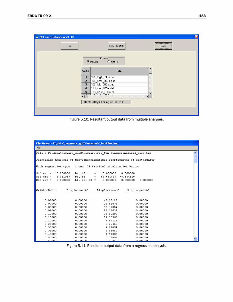
ERDC TR-09-2 153

Figure 5.10. Resultant output data from multiple analyses.

Figure 5.11. Resultant output data from a regression analysis.

ERDC TR-09-2 154

5.3 Example 1 – Single Analysis or Sliding Block Analysis

In this first example, a single acceleration time-history is considered. The tabs that will be used for this example are described in Section 5.2.1. From the File pull-down menu, select Open and accept the file “single_analysis_kcg.nmk”. This particular horizontal earthquake time-history was recorded having a moment magnitude of 6.6. The next step is to decide on the maximum transmissible acceleration or critical accelera-tion used for this analysis. At the Maximum Transmissible Accelera-tion Tab, for a single analysis, select the kc_g option and enter a value of 0.3 with the Acceleration Units as fractional G. Finally, in the Analysis tab (Figure 5.12), set the Output Units to values of inches. Run the analysis by selecting the Run Newmark Analyzer.

Figure 5.12. The Analysis tab for Example 1.

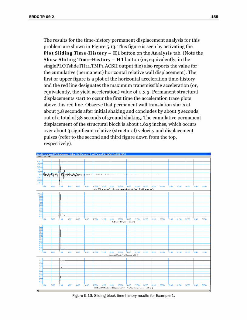
ERDC TR-09-2 155

The results for the time-history permanent displacement analysis for this problem are shown in Figure 5.13. This figure is seen by activating the Plot Sliding Time-History – H1 button on the Analysis tab. (Note the Show Sliding Time-History – H1 button (or, equivalently, in the singlePLOTslideTH11.TMP1 ACSII output file) also reports the value for the cumulative (permanent) horizontal relative wall displacement). The first or upper figure is a plot of the horizontal acceleration time-history and the red line designates the maximum transmissible acceleration (or, equivalently, the yield acceleration) value of 0.3 g. Permanent structural displacements start to occur the first time the acceleration trace plots above this red line. Observe that permanent wall translation starts at about 3.8 seconds after initial shaking and concludes by about 5 seconds out of a total of 38 seconds of ground shaking. The cumulative permanent displacement of the structural block is about 1.625 inches, which occurs over about 3 significant relative (structural) velocity and displacement pulses (refer to the second and third figure down from the top, respectively).

Figure 5.13. Sliding block time-history results for Example 1.

ERDC TR-09-2 156

5.4 Example 2 – Multiple Analyses with Regression using Equation Form Two.

In this second example and with compactness in mind, a set of 10 pairs of baseline corrected acceleration time histories are considered. These sets of horizontal earthquake time histories were recorded on rock and for moment magnitudes in the 7 range.

Starting from the File pull-down menu, select Open and accept the file “multi_10sets_ex2.nmk”. From this input file, the user can browse through data within tabs two through four. Data entry and information regarding these tabs are listed within the multiple analyses segment of Section 5.2.1 and also in Sections 5.2.2 and 5.2.3. Please note that for this example, standardized displacement computations have not been requested.

The next step is to decide on the maximum transmissible acceleration or critical acceleration used for this analysis. From the Maximum Trans-missible Acceleration tab and for multiple analyses, there are 16 kc /km values listed. These values are the default and will be used for this exam-ple. At the Selection of Time Histories tab, all of the various combi-nations will be included for this example.

In the Analysis tab, the regression form type two expression is the equation of choice and the output units will be in inches, as shown in Figure 5.14.

After this selection, run the analysis by selecting the Run Newmark Analyzer.

The results for the time-history permanent displacement analysis for this example 2 can be seen for each individually time-history or set, by activating the Plot Sliding Time-History – H1 or Plot Sliding Time-History – H2 button on the Analysis tab. (Note the Show Sliding Time-History – H1 button (or, equivalently, in the output ASCII texts file as described in Appendix B) also reports the value for the cumulative (permanent) horizontal relative structural displacement).

An observation from viewing the output of the non-dimensionalized displacement of set 1, Figure 5.15, shows for this analysis that the H2(-) graph has the largest magnitude.

ERDC TR-09-2 157

Figure 5.14. The Analysis tab for Example 2.

Upon inspection of the regression analysis for this example 2, Figure 5.16, shows that all of the data below a kc /km value of 0.4 is contained below the curve representing the 95 percent probability of non-exceedance relation-ship. Some of the data greater than a kc /km value of 0.4 does fall above the curve and lies above the 95 percent probability of non-exceedance rela-tionship. An ideal data set would have a few data points falling above the 95 percent probability of non-exceedance relationship for all kc /km data point values. This example illustrates the importance of including larger number of sets of horizontal time histories in order to more efficiently represent the data when performing a regression analysis. As a final note, observe the plotted data from the Introduction tab (Figure 5.1).

ERDC TR-09-2 158

Figure 5.15. Non-dimensionalized earthquake displacements.

The authors of this report believe that the resultant plot from the regres-sion analysis shows a reasonable data set base which results in reasonable statistical relationships for the 122 sets of horizontal earthquake time histories and over the entire range of kc /km data point values.

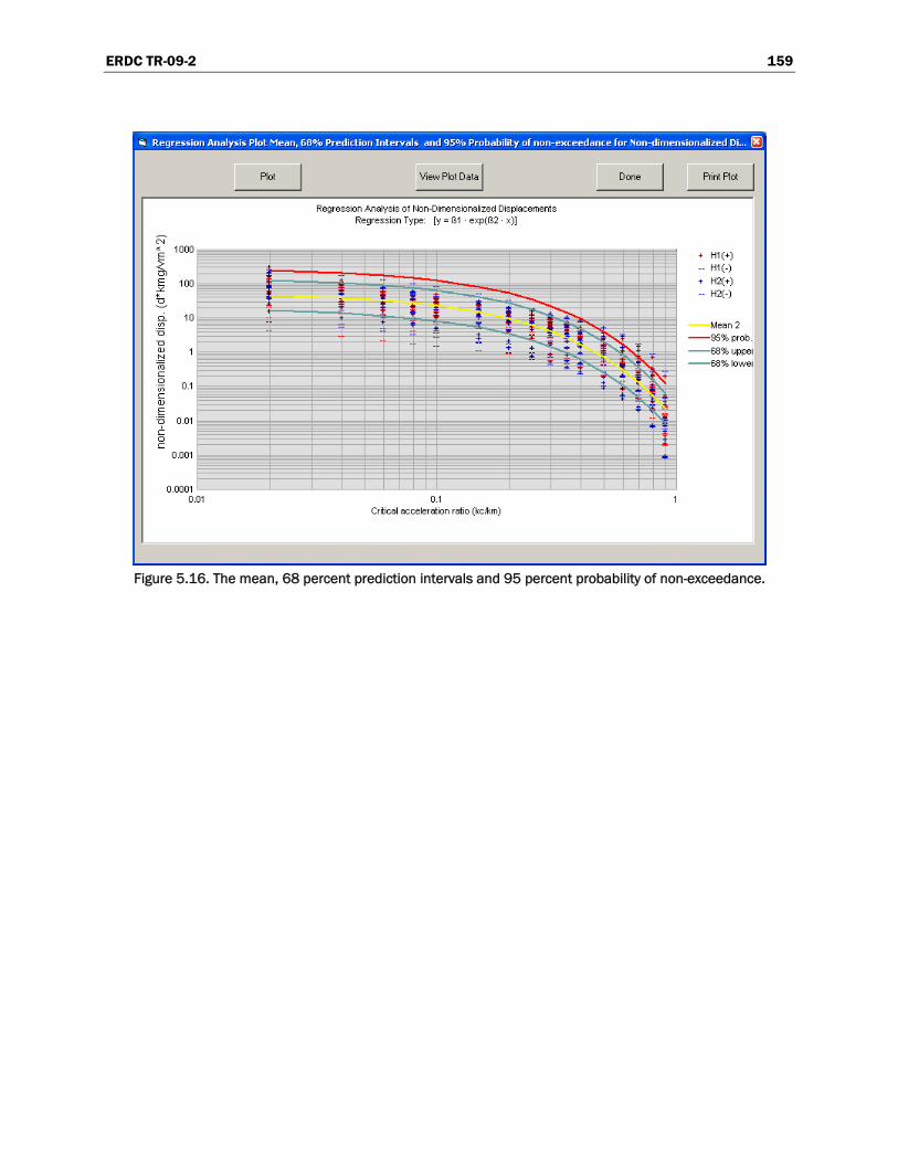
ERDC TR-09-2 159

Figure 5.16. The mean, 68 percent prediction intervals and 95 percent probability of non-exceedance.

ERDC TR-09-2 160

6 Conclusions and Recommendations 6.1 Introduction

This report describes the results of a series of numerical investigations using the PC-based software named Newmark that performs a permanent sliding block displacement analysis. The authors of this report note that baseline corrected acceleration time histories must be used in these per-manent deformation analyses. Newmark can also perform regression analyses in order to develop up to three user selected forms of generalized equations of simplified permanent displacement relationships for sets of user defined acceleration time histories. In Chapter 4, a series of regres-sion analyses were summarized for baseline corrected acceleration time histories recorded on rock for three earthquake moment magnitude Mw ranges of 4.85 to 6.06, 6.06 to 6.8, and 6.9 to 8.1, with average Mw values of 5.6, 6.5, and 7.3 for each of the three groups. An assessment discussed in Chapter 4 concluded that Equation Form Two, the two-term regression results for a form of equation that is linear in natural logarithm trans-formation, provides both the best fit to the (non-dimensionalized) permanent displacement data as well as the lowest order relationship without compromising accuracy. Lastly, as a special case established in Chapter 4, Equation Form Two regression results were evaluated for the entire 122 sets of baseline corrected acceleration time histories recorded on rock, without differentiation of Mw (group four). This chapter sum-marizes the probabilistic relationships derived from Equation Form Two of all four groups of earthquake magnitudes.

6.2 Ninety-five percent probability of non-exceedance

The next four subsections (6.2.1 – 6.2.4) report the 95 percent probability of non-exceedance relationships for each of the three magnitude groups with the last subsection, the fourth group, encompassing all three groups.

6.2.1 Non-dimensionalized displacements of 23 sets of Moment Magnitude 7 group.


ERDC TR-09-2 161

. exp .m m c

mm

d k g kkv

⎛ ⎞• ⎟⎜ ⎟= • − • •⎜ ⎟⎜ ⎟⎜⎝ ⎠2 70 1 9 2 4 64. (bis 4.14)

where:




The corresponding 95 percent probability of non-exceedance permanent displacement relationship is

. exp .mm

m m

vd

kck

g k

⎡ ⎤ ⎛ ⎞⎟⎜⎢ ⎥ ⎟= • • − •⎜ ⎟⎢ ⎥ ⎜ ⎟⎜• ⎝ ⎠⎣ ⎦

2

325 4 9 2 (6.1)


6.2.2 Non-dimensionalized displacements of 38 sets of Moment Magnitude 6 group

The regression analysis of the of the 38 sets of Magnitude 6 rock accel-eration time histories resulted in the non-dimensionalized displacement for 95 percent probability of non-exceedance of

. exp .m m c

mm

d k g kkv

⎛ ⎞• ⎟⎜ ⎟= • − • •⎜ ⎟⎜ ⎟⎜⎝ ⎠2 78 6 9 12 3 68. (bis 4.41)


. exp .mm

m m

vd

kck

g k

⎡ ⎤ ⎛ ⎞⎟⎜⎢ ⎥ ⎟= • • − •⎜ ⎟⎢ ⎥ ⎜ ⎟⎜• ⎝ ⎠⎣ ⎦

2

289 5 9 12 (6.2)

ERDC TR-09-2 162


6.2.3 Non-dimensionalized displacements of 66 sets of Moment Magnitude 5 group


. exp .m m c

mm

d k g kkv

⎛ ⎞• ⎟⎜ ⎟= • − • •⎜ ⎟⎜ ⎟⎜⎝ ⎠2 57 0 8 58 3 39. (bis 4.68)


. exp .mm

m m

vd

kck

g k

⎡ ⎤ ⎛ ⎞⎟⎜⎢ ⎥ ⎟= • • − •⎜ ⎟⎢ ⎥ ⎜ ⎟⎜• ⎝ ⎠⎣ ⎦

2

193 2 8 58 (6.3)


6.2.4 Non-dimensionalized displacements of 122 sets of Moment Magnitude 5 – 7 groups

The regression analysis of the 122 sets of all Magnitudes 5 - 7 of rock accel-eration time histories resulted in the non-dimensionalized displacement for 95 percent probability of non-exceedance of

. exp .m m c

mm

d k g kkv

⎛ ⎞• ⎟⎜ ⎟= • − • •⎜ ⎟⎜ ⎟⎜⎝ ⎠2 65 44 8 86 3 75. (bis 4.87)


. exp .mm

m m

vd

kck

g k

⎡ ⎤ ⎛ ⎞⎟⎜⎢ ⎥ ⎟= • • − •⎜ ⎟⎢ ⎥ ⎜ ⎟⎜• ⎝ ⎠⎣ ⎦

2

245 4 8 86 (6.4)

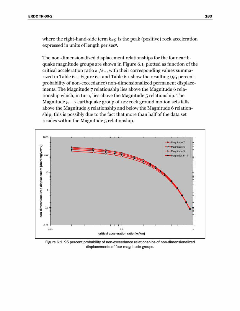
ERDC TR-09-2 163


The non-dimensionalized displacement relationships for the four earth-quake magnitude groups are shown in Figure 6.1, plotted as function of the critical acceleration ratio kc/km, with their corresponding values summa-rized in Table 6.1. Figure 6.1 and Table 6.1 show the resulting (95 percent probability of non-exceedance) non-dimensionalized permanent displace-ments. The Magnitude 7 relationship lies above the Magnitude 6 rela-tionship which, in turn, lies above the Magnitude 5 relationship. The Magnitude 5 – 7 earthquake group of 122 rock ground motion sets falls above the Magnitude 5 relationship and below the Magnitude 6 relation-ship; this is possibly due to the fact that more than half of the data set resides within the Magnitude 5 relationship.

0.01

0.1

1

10

100

1000

0.01 0.1 1


non-

dim

ensi

onal

ized

dis

plac

emen

t [dm

*km

g/vm

^2]

Magnitude 7

Magnitude 6

Magnitude 5

Magitudes 5 - 7

Figure 6.1. 95 percent probability of non-exceedance relationships of non-dimensionalized

displacements of four magnitude groups.

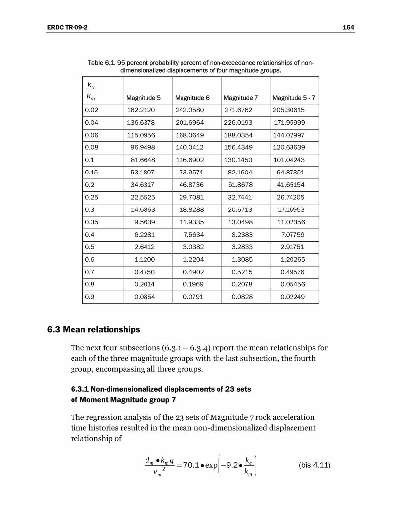
ERDC TR-09-2 164

Table 6.1. 95 percent probability percent of non-exceedance relationships of non-dimensionalized displacements of four magnitude groups.

c

m

kk

Magnitude 5 Magnitude 6 Magnitude 7 Magnitude 5 - 7

0.02 162.2120 242.0580 271.6762 205.30615

0.04 136.6378 201.6964 226.0193 171.95999

0.06 115.0956 168.0649 188.0354 144.02997

0.08 96.9498 140.0412 156.4349 120.63639

0.1 81.6648 116.6902 130.1450 101.04243

0.15 53.1807 73.9574 82.1604 64.87351

0.2 34.6317 46.8736 51.8678 41.65154

0.25 22.5525 29.7081 32.7441 26.74205

0.3 14.6863 18.8288 20.6713 17.16953

0.35 9.5639 11.9335 13.0498 11.02356

0.4 6.2281 7.5634 8.2383 7.07759

0.5 2.6412 3.0382 3.2833 2.91751

0.6 1.1200 1.2204 1.3085 1.20265

0.7 0.4750 0.4902 0.5215 0.49576

0.8 0.2014 0.1969 0.2078 0.05456

0.9 0.0854 0.0791 0.0828 0.02249

6.3 Mean relationships

The next four subsections (6.3.1 – 6.3.4) report the mean relationships for each of the three magnitude groups with the last subsection, the fourth group, encompassing all three groups.

6.3.1 Non-dimensionalized displacements of 23 sets of Moment Magnitude group 7


. exp .m m c

mm

d k g kkv

⎛ ⎞• ⎟⎜ ⎟= • − •⎜ ⎟⎜ ⎟⎜⎝ ⎠2 70 1 9 2 (bis 4.11)

ERDC TR-09-2 165

where:




The corresponding mean permanent displacement relationship is

. exp .mm

m m

vd

kck

g k

⎡ ⎤ ⎛ ⎞⎟⎜⎢ ⎥ ⎟= • • − •⎜ ⎟⎢ ⎥ ⎜ ⎟⎜• ⎝ ⎠⎣ ⎦

2

70 1 9 2 (6.5)



The regression analysis of the of the 38 sets of Magnitude 6 rock accel-eration time histories resulted in the mean non-dimensionalized dis-placement relationship of

. exp .m m c

mm

d k g kkv

⎛ ⎞• ⎟⎜ ⎟= • − •⎜ ⎟⎜ ⎟⎜⎝ ⎠2 78 6 9 12 (bis 4.38)


. exp .mm

m m

vd

kck

g k

⎡ ⎤ ⎛ ⎞⎟⎜⎢ ⎥ ⎟= • • − •⎜ ⎟⎢ ⎥ ⎜ ⎟⎜• ⎝ ⎠⎣ ⎦

2

78 6 9 12 (6.6)


ERDC TR-09-2 166



. exp .m m c

mm

d k g kkv

⎛ ⎞• ⎟⎜ ⎟= • − •⎜ ⎟⎜ ⎟⎜⎝ ⎠2 57 0 8 58 (bis 4.65)


. exp .mm

m m

vd

kck

g k

⎡ ⎤ ⎛ ⎞⎟⎜⎢ ⎥ ⎟= • • − •⎜ ⎟⎢ ⎥ ⎜ ⎟⎜• ⎝ ⎠⎣ ⎦

2

57 0 8 58 (6.7)


6.3.4 Non-dimensionalized displacements of 122 sets of Moment Magnitude 5 – 7 groups

The regression analysis of the 122 sets of Magnitude 5 - 7 rock acceleration time histories resulted in the mean non-dimensionalized displacement relationship of

. exp .m m c

mm

d k g kkv

⎛ ⎞• ⎟⎜ ⎟= • − •⎜ ⎟⎜ ⎟⎜⎝ ⎠2 65 44 8 86 (bis 4.83)


. exp .mm

m m

vd

kck

g k

⎡ ⎤ ⎛ ⎞⎟⎜⎢ ⎥ ⎟= • • − •⎜ ⎟⎢ ⎥ ⎜ ⎟⎜• ⎝ ⎠⎣ ⎦

2

65 44 8 86 (6.8)

where the right-hand-side term kmg is the peak (positive) rock acceleration expressed in units of length per sec2..

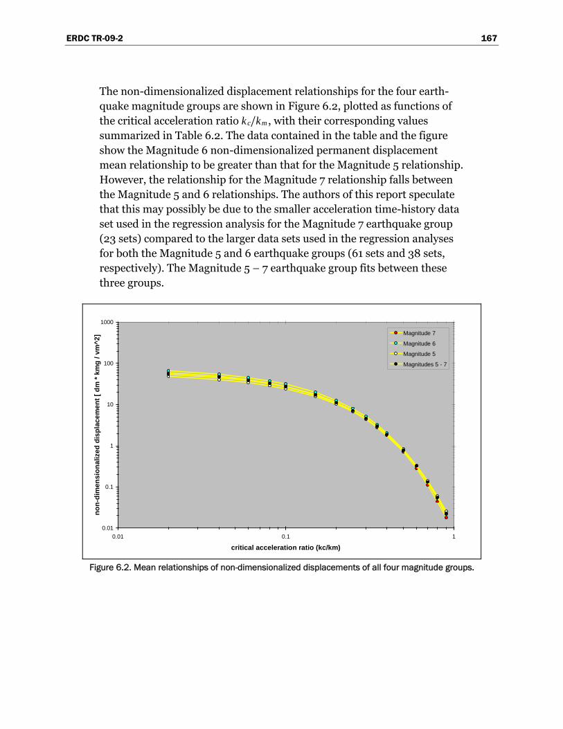
ERDC TR-09-2 167

The non-dimensionalized displacement relationships for the four earth-quake magnitude groups are shown in Figure 6.2, plotted as functions of the critical acceleration ratio kc/km, with their corresponding values summarized in Table 6.2. The data contained in the table and the figure show the Magnitude 6 non-dimensionalized permanent displacement mean relationship to be greater than that for the Magnitude 5 relationship. However, the relationship for the Magnitude 7 relationship falls between the Magnitude 5 and 6 relationships. The authors of this report speculate that this may possibly be due to the smaller acceleration time-history data set used in the regression analysis for the Magnitude 7 earthquake group (23 sets) compared to the larger data sets used in the regression analyses for both the Magnitude 5 and 6 earthquake groups (61 sets and 38 sets, respectively). The Magnitude 5 – 7 earthquake group fits between these three groups.

0.01

0.1

1

10

100

1000

0.01 0.1 1


non-

dim

ensi

onal

ized

dis

plac

emen

t [ d

m *

kmg

/ vm

^2] Magnitude 7

Magnitude 6

Magnitude 5

Magnitudes 5 - 7

Figure 6.2. Mean relationships of non-dimensionalized displacements of all four magnitude groups.

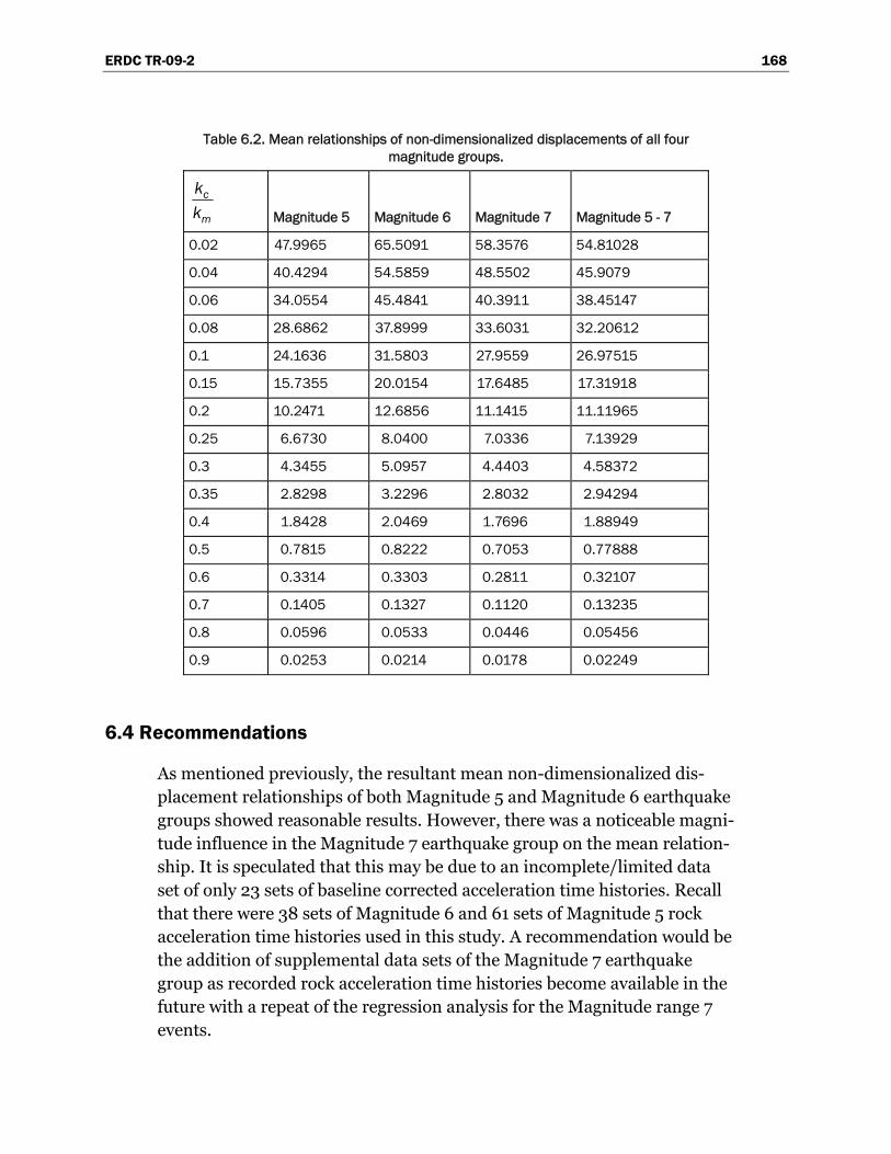
ERDC TR-09-2 168

Table 6.2. Mean relationships of non-dimensionalized displacements of all four magnitude groups.

c

m

kk Magnitude 5 Magnitude 6 Magnitude 7 Magnitude 5 - 7

0.02 47.9965 65.5091 58.3576 54.81028

0.04 40.4294 54.5859 48.5502 45.9079

0.06 34.0554 45.4841 40.3911 38.45147

0.08 28.6862 37.8999 33.6031 32.20612

0.1 24.1636 31.5803 27.9559 26.97515

0.15 15.7355 20.0154 17.6485 17.31918

0.2 10.2471 12.6856 11.1415 11.11965

0.25 6.6730 8.0400 7.0336 7.13929

0.3 4.3455 5.0957 4.4403 4.58372

0.35 2.8298 3.2296 2.8032 2.94294

0.4 1.8428 2.0469 1.7696 1.88949

0.5 0.7815 0.8222 0.7053 0.77888

0.6 0.3314 0.3303 0.2811 0.32107

0.7 0.1405 0.1327 0.1120 0.13235

0.8 0.0596 0.0533 0.0446 0.05456

0.9 0.0253 0.0214 0.0178 0.02249

6.4 Recommendations

As mentioned previously, the resultant mean non-dimensionalized dis-placement relationships of both Magnitude 5 and Magnitude 6 earthquake groups showed reasonable results. However, there was a noticeable magni-tude influence in the Magnitude 7 earthquake group on the mean relation-ship. It is speculated that this may be due to an incomplete/limited data set of only 23 sets of baseline corrected acceleration time histories. Recall that there were 38 sets of Magnitude 6 and 61 sets of Magnitude 5 rock acceleration time histories used in this study. A recommendation would be the addition of supplemental data sets of the Magnitude 7 earthquake group as recorded rock acceleration time histories become available in the future with a repeat of the regression analysis for the Magnitude range 7 events.

ERDC TR-09-2 169

References Ambraseys, N. N., and J. M. Menu. 1988. Earthquake-induced ground displacements.

Earthquake Engineering and Structural Dynamics. 16:985–1006.

American Society of Civil Engineers (ASCE) Standard. 1986. Seismic analysis of safety-related nuclear structures and commentary on Standard for Seismic Analysis of Safety Related Nuclear Structures. 004-98. New York: ASCE.

Cai, Z., and R. J. Bathurst. 1996. Deterministic sliding block methods for estimating seismic displacements of earth structures. Soil Dynamics and Earthquake Engineering 15:255–268.

Clough, G. W., and J. M. Duncan. 1969. Finite element analyses of Port Allen and Old River Locks. Contract Report S-69-6. Vicksburg, MS: U.S. Army Engineer Waterways Experiment Station.

______. 1991. Earth Pressures, Chapter 6. In Foundation Engineering Handbook, 2nd ed., ed. H. Y. Fang, 223–235.New York: Van Nostrand Reinhold.

Ebeling, R. M. 1992. Introduction to the computation of response spectrum for earthquake engineering. Technical Report ITL-92-4. Vicksburg, MS: U.S. Army Engineer Waterways Experiment Station.

Ebeling, R. M., and A. Chase. Translational response of rock-founded gravity dams to earthquake ground motions using CorpsDamSlip (CDSlip) (in preparation). Vicksburg, MS: U.S. Army Engineer Research and Development Center.

Ebeling, R. M., and E. E. Morrison. 1992. The seismic design of waterfront retaining structures. Technical Report ITL-92-11. Vicksburg, MS: U.S. Army Waterways Experiment Station.

Ebeling, R. M., and R. L. Mosher. 1996. Red River U-Frame Lock No. 1, Backfill-structure-foundation interaction. ASCE Journal of Geotechnical Engineering 122(3):216–225.

Ebeling, R. M., and R. E. Wahl. 1997. Soil-structure-foundation interaction analysis of new roller-compacted concrete north lock wall at McAlpine Locks. Technical Report ITL-97-5. Vicksburg, MS: U.S. Army Engineer Waterways Experiment Station.

Ebeling, R. M., and B. C. White. 2006. The rotational response of toe-restrained retain-ing walls to earthquake ground motions. ERDC/ITL TR-06-2. Vicksburg, MS: U.S. Army Engineer Research and Development Center

Ebeling, R. M., J. F. Peters, and G. W. Clough. 1992. Users Guide for the incremental construction, soil-structure interaction program SOILSTRUCT. Technical Report ITL-90-6. Vicksburg, MS: U.S. Army Waterways Experiment Station.

ERDC TR-09-2 170

Ebeling, R. M., R. L. Mosher, K. Abraham, and J. F. Peters. 1993. Soil-structure inter-action study of Red River Lock and Dam No. 1 subjected to sediment loading. Technical Report ITL-93-3. Vicksburg, MS: U.S. Army Engineer Waterways Experiment Station.

Ebeling, R. M., R. A. Green, and S. E. French. 1997a. Accuracy of response of single-degree-of-freedom systems to ground motion. Technical Report ITL-97-7. Vicksburg, MS: U.S. Army Engineer Waterways Experiment Station

Ebeling, R. M., M. E. Pace, and E. E. Morrison. 1997b. Evaluating the stability of existing massive concrete gravity structures founded on rock. Technical Report REMR-CS-54. Vicksburg, MS: U.S. Army Engineer Waterways Experiment Station.

Ebeling, R. M., J. F. Peters, and R. L. Mosher. 1997c. The role of non-linear deformation analyses in the design of a reinforced soil berm at Red River U-Frame Lock No. 1. International Journal for Numerical and Analytical Methods in Geomechanics 21:753–787.

Ebeling, R. M., A. Chase, and B. C. White. 2007. Translational response of toe-restrained retaining walls to earthquake ground motions using CorpsWallSlip (CWSlip). ERDC/ITL TR-07-1. Vicksburg, MS: U.S. Army Engineer Research and Develop-ment Center.

Franklin, A. G., and F. K. Chang. 1977. Earthquake resistance of earth and rockfill dams: Report 5: Permanent displacement of earth embankments by Newmark sliding block analysis. Miscellaneous Paper S-71-17. Vicksburg, MS: U.S. Army Water-ways Experiment Station.

Green, R. A., and R. M. Ebeling. 2002. Seismic analysis of cantilever retaining walls, Phase I. ERDC/ITL TR-02-3. Vicksburg, MS: U.S. Army Engineer Research and Development Center.

Headquarters, U.S. Army Corps of Engineers. 1989. Retaining and flood walls. EM 1110-2-2502.Washington, DC.

Headquarters, Department of the Army. 1995. Earthquake design and evaluation for civil works projects. ER 1110-2-1806. Washington, DC.

______. 2005. Stability analysis of concrete structures. EM 1110-2-2100. Washington, DC.

Hynes-Griffin, M. E., and A. G. Franklin. 1984. Rationalizing the seismic coefficient method. Miscellaneous Paper GL-84-13. Vicksburg, MS: U.S. Army Engineer Waterways Experiment Station.

Idriss, I. M. 1985. Evaluating seismic risk in engineering practice. In Proceeding, 11th International Conference on Soil Mechanics and Foundation Engineering 1:255–320.

Lysmer, J., T. Udaka, C.-F. Tsai, and H. B. Seed. 1975. FLUSH - A computer program for approximate 3-D analysis of soil-structure interaction problems. Report No. EERC 75-30. Berkley, CA: Earthquake Engineering Research Center, University of California, Berkeley.

ERDC TR-09-2 171

Makdisi, F. I., and H. B. Seed. 1978. Simplified procedure for estimating dam and embankment earthquake-induced deformations. Journal of the Geotechnical Engineering Division, ASCE, 104(GT7):849–867.

Mononobe, N., and H. Matsuo. 1929. On the determination of earth pressures during earthquakes. In Proceedings, World Engineering Congress 9:177–185.

Newmark, N. 1965. Effects of earthquakes on dams and embankments. Geotechnique 15(2):139–160.

Okabe, S. 1924. General theory of earth pressures and seismic stability of retaining walls. Journal Japan Society of Civil Engineering 10(6).

______. 1926. General theory of earth pressures. Journal Japan Society of Civil Engineering 12(1).

Richards, R., Jr., and D. Elms. 1979. Seismic behavior of gravity retaining walls. Journal of Geotechnical Engineering Division, ASCE, 105(GT4):449–464.

Schnabel, P. B., J. Lysmer, and H. B. Seed. 1972. SHAKE: A computer program for earthquake response analysis of horizontally layered sites. Report EERC-72-12. Berkley, CA: Earthquake Engineering Research Center, University of California, Berkeley.

Steedman, R. S., and X. Zeng. 1996. Rotation of large gravity walls on rigid foundations under seismic loading. In Proceedings, Analysis and Design of Retaining Struc-tures Against Earthquakes. ASCE Geotechnical Special Publication No. 60. ed., S. Prakash, 38-56. Soil Dynamics Committee of the Geo-Institute of ASCE.

Strom, R. W., and R. M. Ebeling. 2004. Simplified methods used to estimate the limit state axial load capacity of spillway invert slabs. ERDC/ITL TR-04-3. Vicksburg, MS: U.S. Army Engineer Research and Development Center.

Whitman, R. V. 1990. Seismic design behavior of gravity retaining walls. Proceedings of ASCE Specialty Conference on Design and Performance of Earth Retaining Structures. Geotechnical Special Publication No. 25:817–842.

Whitman, R. V., and S. Liao. 1985a. Seismic design of retaining walls. Miscellaneous Paper GL-85-1. Vicksburg, MS: U.S. Army Engineer Waterways Experiment Station.

______. 1985b. Seismic design of gravity retaining walls. Proc. 8th World Conference on Earthquake Engineering, San Francisco 3:533–540.

______. 2000. Fifty years of soil dynamics. Fifteenth Nabor Carrillo Lecture. Delivered during the XX National Meeting of Soil Mechanics, Oaxaca, Mexico, November 2000. 88 p.

Wong, C. 1982. Seismic analysis and improved seismic design procedure for gravity retaining walls. Research Report 82-32. Cambridge, MA: Department of Civil Engineering, Massachusetts Institute of Technology.

ERDC TR-09-2 172

Zeng, X., and R. S. Steedman. 2000. Rotating block method for seismic displacement of gravity walls. ASCE Journal of Geotechnical and Geoenvironmental Engineering 126(8):709–717.

ERDC TR-09-2 173

Appendix A: Listing and Description of the Newmark ASCII Input Data File (file name: Newmark.in) A.1 Introduction

This appendix lists and describes the contents of the ASCII input data file to the FORTRAN engineering computer program portion of Newmark. This input data file, always designated as Newmark.in, is created by the graphical user interface (GUI), the visual modeler portion of Newmark. The FORTRAN code of Newmark evolved from CorpsWallRotate_Wet (Ebeling et al. 2007)1 which encompasses similar engineering concepts and computations.

The ASCII input data to Newmark is provided in 6 groups of data. They are as follows:

A.2 Group 1 – Designate the type of Newmark Analysis

KEY_NEWMARK_Analysis

with

KEY_NEWMARK_Analysis = 1, Single Newmark analysis using one horizontal acceleration time-history.

= 2, Multiple Newmark time history analyses using multiple acceleration time histories are required.

A.3 Group 2 – Designate global parameters and horizontal components with the input listed in two parts

1Note: Part 1 will be skipped for a single Newmark analysis (KEY_NEWMARK_Analysis = 1)

Part 1: Key_GlobalAccVel 1 All references cited in this appendix are included in the Reference section at the end of the main text.

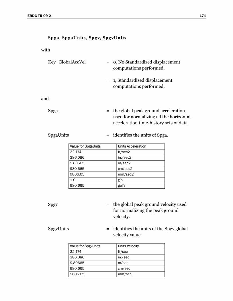
ERDC TR-09-2 174

Spga, SpgaUnits, Spgv, SpgvUnits

with

Key_GlobalAccVel = 0, No Standardized displacement computations performed.

= 1, Standardized displacement computations performed.

and

Spga = the global peak ground acceleration used for normalizing all the horizontal acceleration time-history sets of data.

SpgaUnits = identifies the units of Spga.

Value for SpgaUnits Units Acceleration 32.174 ft/sec2 386.086 in./sec2 9.80665 m/sec2 980.665 cm/sec2 9806.65 mm/sec2 1.0 g’s 980.665 gal’s

Spgv = the global peak ground velocity used for normalizing the peak ground velocity.

SpgvUnits = identifies the units of the Spgv global velocity value.

Value for SpgvUnits Units Velocity 32.174 ft/sec 386.086 in./sec 9.80665 m/sec 980.665 cm/sec 9806.65 mm/sec

ERDC TR-09-2 175

Note: Second Row of Part 1 data will not be read when no standardized displacement computations are to be performed. (Key_GlobalAccVel = 0)

Part 2: TH_State, Nset, H1set, H2set

with

TH_State = 1, time-history for horizontal component 1.

= 2, time-history for horizontal component 2.

= 3, both time-histories for horizontal components 1 & 2.

Always used for multiple time-history analyses.

Nset = the overall number of sets of horizontal components

H1set = the number of sets available for horizontal component 1

H2set = the number of sets available for horizontal component 2

Depending on the value of TH_State, the following input will either have one or two filenames.

A.4 Group 3 –Time-history information with input listed in two parts

Part 1: Acceleration time-history parameters and data for horizontal component 1

Note: For TH_State=2, the time-history information will be specified for horizontal component 2 and Part 2 will be omitted.

The data given in the following two sections list the acceleration time-history file[s] and summarize the parameters used to characterize each

ERDC TR-09-2 176

acceleration time-history. The horizontal component[s] evaluated will be dependent on the values of TH_State and Nset of information.

Section 1: SetId, DT, GACC, Xscale, NheaderLines, NvalsPerLine, DataFmt

H1_TimehistoryFile

with

SetId = the index of Nset (i.e., 1, 2, … to Nset, sequentially).

DT = the time step in seconds.

GACC = the constant of acceleration due to gravity. The value for GACC identifies the units of acceleration, velocity and intrinsic displacement according to following tabulation.

Value for GACC Units of Acceleration Units of Velocity Units of Intrinsic Displacement

32.174 ft/sec2 ft/sec feet

386.086 in./sec2 in./sec inches

9.80665 m/sec2 m/sec meters

980.665 cm/sec2 cm/sec centimeters

9806.65 mm/sec2 mm/sec millimeters


Xscale = the scale factor applied to the horizontal acceleration time history (negative value when time-history is inverted).

NheaderLines = number of header lines within the H1_TimehistoryFile.

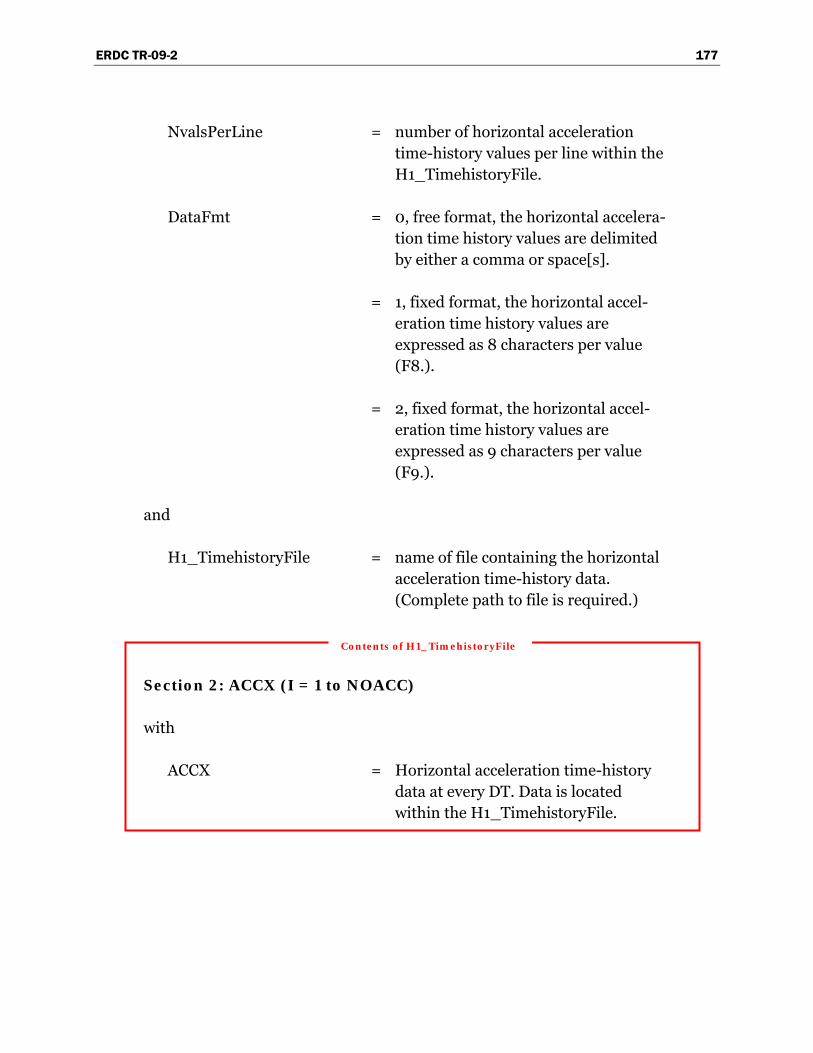
ERDC TR-09-2 177

NvalsPerLine = number of horizontal acceleration time-history values per line within the H1_TimehistoryFile.

DataFmt = 0, free format, the horizontal accelera-tion time history values are delimited by either a comma or space[s].

= 1, fixed format, the horizontal accel-eration time history values are expressed as 8 characters per value (F8.).

= 2, fixed format, the horizontal accel-eration time history values are expressed as 9 characters per value (F9.).

and

H1_TimehistoryFile = name of file containing the horizontal acceleration time-history data. (Complete path to file is required.)

Section 2: ACCX (I = 1 to NOACC)

with

ACCX = Horizontal acceleration time-history data at every DT. Data is located within the H1_TimehistoryFile.

Contents of H1_TimehistoryFile

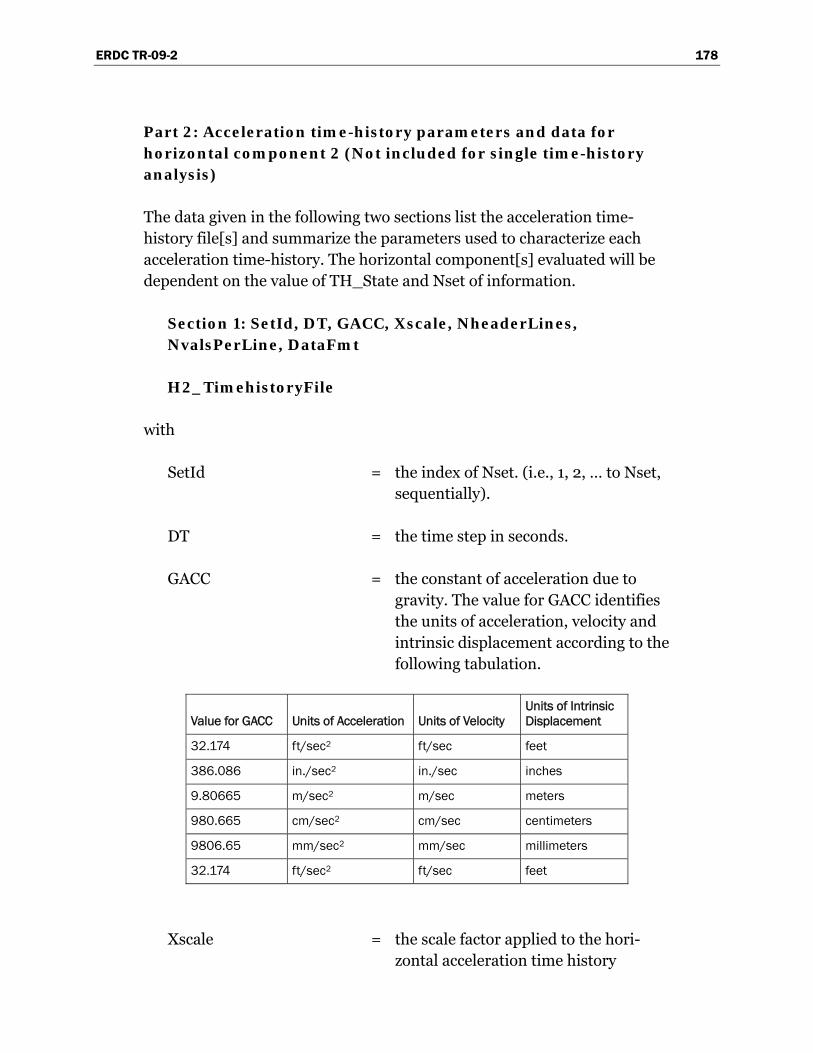
ERDC TR-09-2 178

Part 2: Acceleration time-history parameters and data for horizontal component 2 (Not included for single time-history analysis)

The data given in the following two sections list the acceleration time-history file[s] and summarize the parameters used to characterize each acceleration time-history. The horizontal component[s] evaluated will be dependent on the value of TH_State and Nset of information.

Section 1: SetId, DT, GACC, Xscale, NheaderLines, NvalsPerLine, DataFmt

H2_TimehistoryFile

with

SetId = the index of Nset. (i.e., 1, 2, … to Nset, sequentially).

DT = the time step in seconds.

GACC = the constant of acceleration due to gravity. The value for GACC identifies the units of acceleration, velocity and intrinsic displacement according to the following tabulation.

Value for GACC Units of Acceleration Units of Velocity Units of Intrinsic Displacement







Xscale = the scale factor applied to the hori-zontal acceleration time history

ERDC TR-09-2 179

(negative value when time-history is inverted).

NheaderLines = number of header lines within the H2_TimehistoryFile.

NvalsPerLine = number of horizontal acceleration values per line within the H2_TimehistoryFile.

DataFmt = 0, free format, the horizontal accel-eration time-history values are delimited by either a comma or space[s].

= 1, fixed format, the horizontal acceler-ation time-history values are expressed as 8 characters per value (F8.).

= 2, fixed format, the horizontal acceler-ation time-history values are expressed as 9 characters per value (F9.).

and

H2_TimehistoryFile = name of file containing the horizontal acceleration time-history data. (Complete path to file is required.)

Section 2: ACCX (I = 1 to NOACC)

with

ACCX = Horizontal acceleration time-history data at every DT. Data is located within the H2_TimehistoryFile.

Contents of H2_TimehistoryFile

Note: Values for the horizontal accelerations used in NEWMARK are equal to ACCX(I) times XSCALE times GACC.

ERDC TR-09-2 180

A.5 Group 4 – Regression Analysis for multiple acceleration time histories with input listed in two parts

Note: For a single Newmark analysis (KEY_NEWMARK_Analysis = 1) there will be no regression analysis: Group 4 will be skipped.

Part 1: KEY_REGRESSION

with

KEY_REGRESSION = 0, No Regression Analyses performed. (Default)

= 1, Common Log transformation for estimation of two parameters (β4, β5)

= 2, Natural Log transformation for estimation of two parameters (β1, β2)

= 3, Natural Log transformation for estimation of three parameters (β1, β2, β3)

= 4, combination of KEY_REGRESSION 1 & 2



= 7, combination of KEY_REGRESSION 1 & 2 & 3

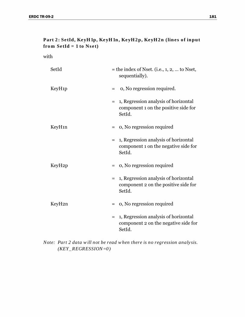
ERDC TR-09-2 181

Part 2: SetId, KeyH1p, KeyH1n, KeyH2p, KeyH2n (lines of input from SetId = 1 to Nset)

with

SetId = the index of Nset. (i.e., 1, 2, … to Nset, sequentially).

KeyH1p = 0, No regression required.

= 1, Regression analysis of horizontal component 1 on the positive side for SetId.

KeyH1n = 0, No regression required

= 1, Regression analysis of horizontal component 1 on the negative side for SetId.

KeyH2p = 0, No regression required

= 1, Regression analysis of horizontal component 2 on the positive side for SetId.

KeyH2n = 0, No regression required

= 1, Regression analysis of horizontal component 2 on the negative side for SetId.

Note: Part 2 data will not be read when there is no regression analysis. (KEY_REGRESSION=0)

ERDC TR-09-2 182

A.6 Group 5 – The classification and value[s] of the Maximum Transmissible Acceleration provide input in two parts, with part 2 only valid for Crit_Acc_State = 2.

Part 1: Crit_Acc_State, Crit_Acc_Units, Crit_Acc_Value

with

Crit_Acc_State = 1, value of ( )ck g , the maximum

transmissible acceleration

with

Crit_Acc_Units = identifies the units of the maximum transmissible acceleration ( )ck g or

input variable Crit_Acc_Value.

Value for Crit_Acc_Units Units Acceleration 32.174 ft/sec2

386.086 in./sec2

9.80665 m/sec2

980.665 cm/sec2

9806.65 mm/sec2

1.0 g’s 980.665 gal’s

and

Crit_Acc_Value = ck g , the maximum transmissible

acceleration.

or

Crit_Acc_State = 2, value[s] of ⎟⎟⎠

⎞⎜⎜⎝

⎛

m

c

kk

, the ratio of the

maximum transmissible acceleration value for the retaining wall ( )ck g and

the peak ground acceleration( )mk g .

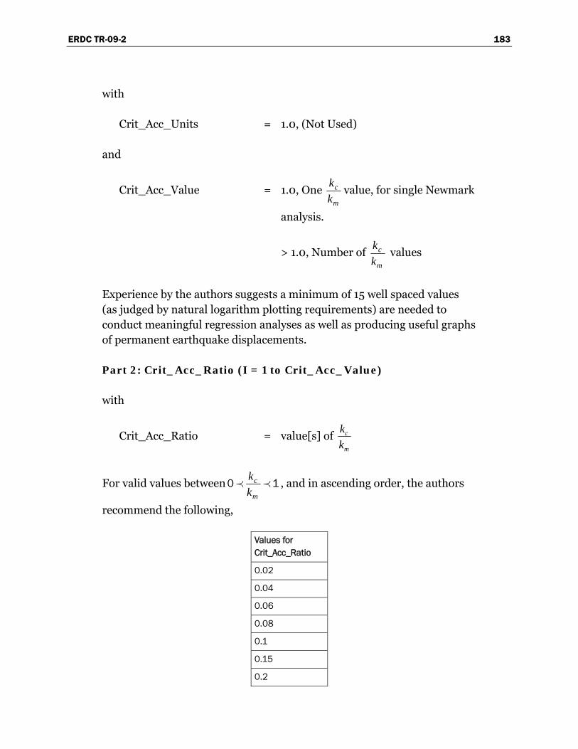
ERDC TR-09-2 183

with

Crit_Acc_Units = 1.0, (Not Used)

and

Crit_Acc_Value = 1.0, One c

m

kk

value, for single Newmark

analysis.

> 1.0, Number of c

m

kk

values

Experience by the authors suggests a minimum of 15 well spaced values (as judged by natural logarithm plotting requirements) are needed to conduct meaningful regression analyses as well as producing useful graphs of permanent earthquake displacements.

Part 2: Crit_Acc_Ratio (I = 1 to Crit_Acc_Value)

with

Crit_Acc_Ratio = value[s] of m

c

kk

For valid values between c

m

kk

0≺ ≺1 , and in ascending order, the authors

recommend the following,

Values for Crit_Acc_Ratio

0.02

0.04

0.06

0.08

0.1

0.15

0.2

ERDC TR-09-2 184

0.25

0.3

0.35

0.4

0.5

0.6

0.7

0.8

0.9

A.7 Group 6 – Designate the output units for computed displacements.

DISPACC

with

DISPACC = identifies the units of the scaled acceleration, computed velocity and computed displacements according to the following tabulation in a Complete Time-History Analysis.

Value for DISPACC Units of Acceleration Units of Velocity

Units of Displacement






ERDC TR-09-2 185

Appendix B: Listing of Newmark ASCII Data Output Files

This appendix lists the Newmark ASCII Output Data Files. Table B.1 lists the output box labels and corresponding files for the visual modeler analysis tabs and briefly describes the contents.

Table B.1. Output data files used by output buttons in the visual modeler analysis tab.

Visual Modeler View Output Label Name of File Description Show Log of Newmark Execution

Newmark.run Displays a listing of the runtime execution process.

Show Input Echo of Newmark Execution

Newmark.out Displays a listing of the input as read from Newmark.in

Plot Time Histories AccX – H1

PLOTaccX1[xxxx].TMP[1/2] StandardizedPlotaccX1[xxxx].TMP[1/2]

Scaled acceleration time-history for horizontal component 1. For a standardized displacement computation, a corresponding file for horizontal component 1 with the standardized computations will be provided.

Plot Time Histories AccX – H2

PLOTaccX2[xxxx].TMP[1/2] StandardizedPlotaccX2[xxxx].TMP[1/2]

Scaled acceleration time-history for horizontal component 2. For a standardized displacement computation, a corresponding file for horizontal component 2 with the standardized computations will be provided.

Plot Sliding Time- History – H1

PLOTslideTH1[xxxx].TMP[1/2] StandardizedPLOTslideTH1[xxxx].TMP[1/2] SinglePLOTslideTH11.TMP[1/2]

Time-history of sliding block analysis for horizontal component 1. For a standardized displacement computation, a corresponding file for horizontal component 1 with the standardized computations will be provided. For a single analysis, and with the critical acceleration as a fractional g.

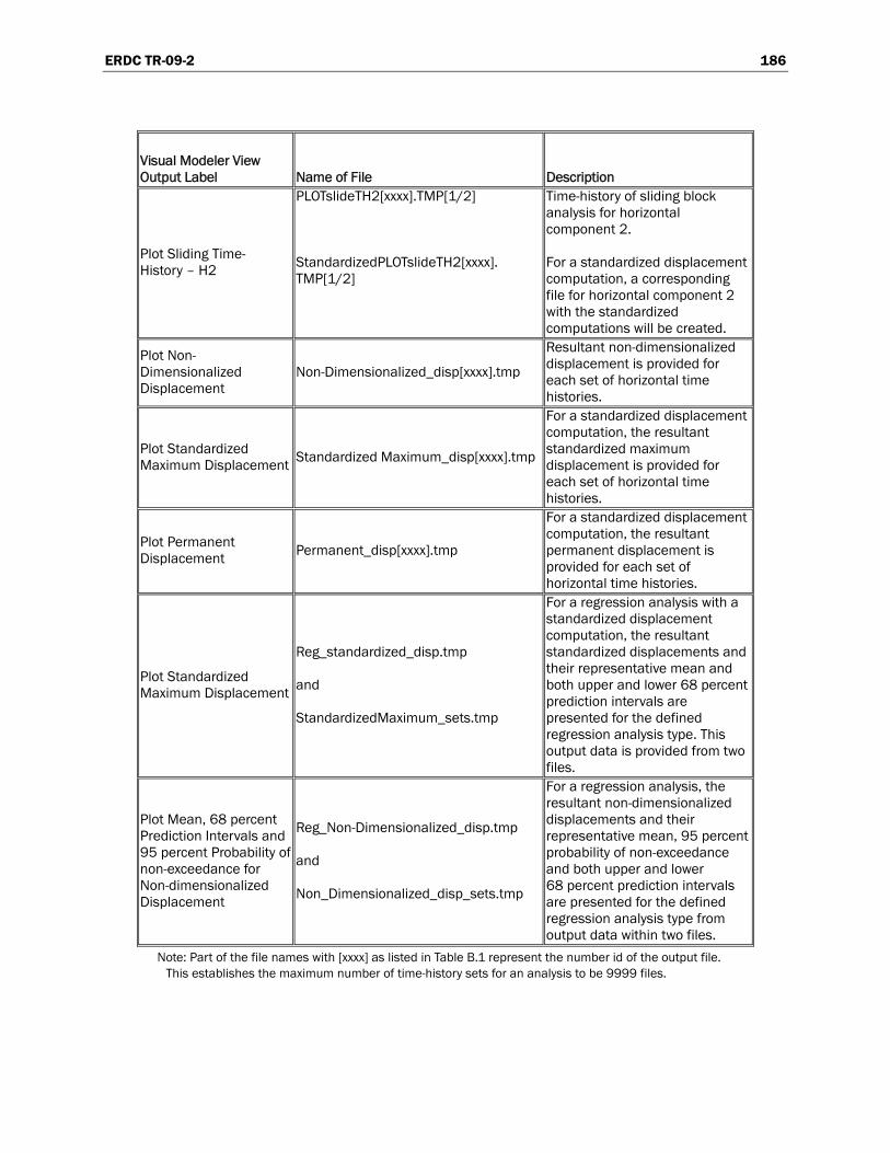
ERDC TR-09-2 186

Visual Modeler View Output Label Name of File Description

Plot Sliding Time- History – H2

PLOTslideTH2[xxxx].TMP[1/2] StandardizedPLOTslideTH2[xxxx]. TMP[1/2]

Time-history of sliding block analysis for horizontal component 2. For a standardized displacement computation, a corresponding file for horizontal component 2 with the standardized computations will be created.

Plot Non-Dimensionalized Displacement

Non-Dimensionalized_disp[xxxx].tmp

Resultant non-dimensionalized displacement is provided for each set of horizontal time histories.

Plot Standardized Maximum Displacement Standardized Maximum_disp[xxxx].tmp

For a standardized displacement computation, the resultant standardized maximum displacement is provided for each set of horizontal time histories.

Plot Permanent Displacement Permanent_disp[xxxx].tmp

For a standardized displacement computation, the resultant permanent displacement is provided for each set of horizontal time histories.

Plot Standardized Maximum Displacement

Reg_standardized_disp.tmp and StandardizedMaximum_sets.tmp

For a regression analysis with a standardized displacement computation, the resultant standardized displacements and their representative mean and both upper and lower 68 percent prediction intervals are presented for the defined regression analysis type. This output data is provided from two files.

Plot Mean, 68 percent Prediction Intervals and 95 percent Probability of non-exceedance for Non-dimensionalized Displacement

Reg_Non-Dimensionalized_disp.tmp and Non_Dimensionalized_disp_sets.tmp

For a regression analysis, the resultant non-dimensionalized displacements and their representative mean, 95 percent probability of non-exceedance and both upper and lower 68 percent prediction intervals are presented for the defined regression analysis type from output data within two files.

Note: Part of the file names with [xxxx] as listed in Table B.1 represent the number id of the output file. This establishes the maximum number of time-history sets for an analysis to be 9999 files.

REPORT DOCUMENTATION PAGE Form Approved

OMB No. 0704-0188 Public reporting burden for this collection of information is estimated to average 1 hour per response, including the time for reviewing instructions, searching existing data sources, gathering and maintaining the data needed, and completing and reviewing this collection of information. Send comments regarding this burden estimate or any other aspect of this collection of information, including suggestions for reducing this burden to Department of Defense, Washington Headquarters Services, Directorate for Information Operations and Reports (0704-0188), 1215 Jefferson Davis Highway, Suite 1204, Arlington, VA 22202-4302. Respondents should be aware that notwithstanding any other provision of law, no person shall be subject to any penalty for failing to comply with a collection of information if it does not display a currently valid OMB control number. PLEASE DO NOT RETURN YOUR FORM TO THE ABOVE ADDRESS.

1. REPORT DATE (DD-MM-YYYY) February 2009

2. REPORT TYPE Final report

3. DATES COVERED (From - To)

5a. CONTRACT NUMBER

5b. GRANT NUMBER

4. TITLE AND SUBTITLE


5c. PROGRAM ELEMENT NUMBER

5d. PROJECT NUMBER

5e. TASK NUMBER

6. AUTHOR(S)

Robert M. Ebeling, Moira T. Fong, Donald E. Yule, Amos Chase, Sr., and Raju V. Kala

5f. WORK UNIT NUMBER 142082

7. PERFORMING ORGANIZATION NAME(S) AND ADDRESS(ES) 8. PERFORMING ORGANIZATION REPORT NUMBER

U.S. Army Engineer Research and Development Center Information Technology Laboratory and Geotechnical and Structures Laboratory 3909 Halls Ferry Road, Vicksburg, MS 39180-6199; Science Applications International Corporation 3532 Manor Drive, Suite 4, Vicksburg, MS 39180

ERDC TR-09-2

9. SPONSORING / MONITORING AGENCY NAME(S) AND ADDRESS(ES) 10. SPONSOR/MONITOR’S ACRONYM(S)

11. SPONSOR/MONITOR’S REPORT NUMBER(S)

Headquarters, U.S. Army Corps of Engineers Washington, DC 20314-1000

12. DISTRIBUTION / AVAILABILITY STATEMENT

Approved for public release; distribution is unlimited.

13. SUPPLEMENTARY NOTES

14. ABSTRACT

This research report describes the engineering formulation and corresponding software developed for the translational response of rock-founded structural systems to earthquake ground motions. The PC software Newmark (and NewmarkVM) is developed to perform an analysis of the permanent sliding displacement response for a structural system founded on rock for a user specified earthquake acceleration time history via a Complete Time History Analysis, also know as the Newmark sliding block method of analysis. The PC-based program Newmark performs a permanent sliding block displacement analysis given a baseline corrected rock site-specific acceleration time history. Newmark can also conduct regression analyses for sets of rock founded acceleration time histories in order to develop up to three user selected forms of generalized equations of simplified permanent displacement relationships. The rock-founded structural system can be a variety of structural feature types; a concrete gravity dam, a concrete monolith, a retaining wall, etc.

(Continued)

15. SUBJECT TERMS Baseline corrected Maximum transmissible acceleration

Newmark sliding block analysis Permanent displacement Rock

Rock earthquake ground motions Seismic Translation

Yield Acceleration

16. SECURITY CLASSIFICATION OF: 17. LIMITATION OF ABSTRACT

18. NUMBER OF PAGES

19a. NAME OF RESPONSIBLE PERSON

a. REPORT

UNCLASSIFIED

b. ABSTRACT

UNCLASSIFIED

c. THIS PAGE

UNCLASSIFIED 203 19b. TELEPHONE NUMBER (include area code)

Standard Form 298 (Re . 8-98) vPrescribed by ANSI Std. 239.18

14. ABSTRACT (Concluded).

The results of the regression analyses discussed in this report resulted in Simplified permanent displacement relationships that were developed using data generated by Newmark for an extensive data base of 122 sets of baseline corrected rock acceleration time histories in the moment magnitude 5 to 7 range. The resulting simplified permanent displacement relationships allow the engineer to rapidly determine the earthquake-induced permanent displacement for a given rock-founded structural system. This alternative procedure requires only rudimentary design/analysis ground motion characterization and use of a simplified permanent seismic displacement relationship for a sliding block (structural) system model. The resulting simplified permanent displacement relationships dis-cussed in this report are being implemented in other Corps permanent (seismically-induced) displacement software such as CorpsWallSlip, and CorpsDamSlip.

ERDC TR-09-2, Permanent Seismically Induced Displacement ...ware Newmark and Newmark. VM. are...

Documents

Transcript of ERDC TR-09-2, Permanent Seismically Induced Displacement ...ware Newmark and Newmark. VM. are...