
Erasure Coding for Big-data Systems: Theory and Practice · PDF file1 Abstract Erasure Coding...
165
Erasure Coding for Big-data Systems: Theory and Practice Rashmi Vinayak Electrical Engineering and Computer Sciences University of California at Berkeley Technical Report No. UCB/EECS-2016-155 http://www2.eecs.berkeley.edu/Pubs/TechRpts/2016/EECS-2016-155.html September 14, 2016
Transcript of Erasure Coding for Big-data Systems: Theory and Practice · PDF file1 Abstract Erasure Coding...

Erasure Coding for Big-data Systems: Theory and Practice
Rashmi Vinayak
Electrical Engineering and Computer SciencesUniversity of California at Berkeley
Technical Report No. UCB/EECS-2016-155http://www2.eecs.berkeley.edu/Pubs/TechRpts/2016/EECS-2016-155.html
September 14, 2016

Copyright © 2016, by the author(s).All rights reserved.
Permission to make digital or hard copies of all or part of this work forpersonal or classroom use is granted without fee provided that copies arenot made or distributed for profit or commercial advantage and that copiesbear this notice and the full citation on the first page. To copy otherwise, torepublish, to post on servers or to redistribute to lists, requires priorspecific permission.

Erasure Coding for Big-data Systems: Theory and Practice
by
Rashmi Korlakai Vinayak
A dissertation submitted in partial satisfaction of the
requirements for the degree of
Doctor of Philosophy
in
Engineering – Electrical Engineering and Computer Sciences
in the
Graduate Division
of the
University of California, Berkeley
Committee in charge:
Professor Kannan Ramchandran, ChairProfessor Ion StoicaProfessor Randy Katz
Professor Rhonda Righter
Fall 2016

Erasure Coding for Big-data Systems: Theory and Practice
Copyright 2016
by
Rashmi Korlakai Vinayak

1
Abstract
Erasure Coding for Big-data Systems: Theory and Practice
by
Rashmi Korlakai Vinayak
Doctor of Philosophy in Engineering – Electrical Engineering and Computer Sciences
University of California, Berkeley
Professor Kannan Ramchandran, Chair
Big-data systems enable storage and analysis of massive amounts of data, and are fuel-ing the data revolution that is impacting almost all walks of human endeavor today. Thefoundation of any big-data system is a large-scale, distributed, data storage system. Thesestorage systems are typically built out of inexpensive and unreliable commodity components,which in conjunction with numerous other operational glitches make unavailability eventsthe norm rather than the exception.
In order to ensure data durability and service reliability, data needs to be stored redun-dantly. While the traditional approach towards this objective is to store multiple replicasof the data, today’s unprecedented data growth rates mandate more e�cient alternatives.Coding theory, and erasure coding in particular, o↵ers a compelling alternative by makingoptimal use of the storage space. For this reason, many data-center scale distributed stor-age systems are beginning to deploy erasure coding instead of replication. This paradigmshift has opened up exciting new challenges and opportunities both on the theoretical aswell as the system design fronts. Broadly, this thesis addresses some of these challenges andopportunities by contributing in the following two areas:
• Resource-e�cient distributed storage codes and systems: Although traditionalerasure codes optimize the usage of storage space, they result in a significant increase inthe consumption of other important cluster resources such as the network bandwidth,input-output operations on the storage devices (I/O), and computing resources (CPU).This thesis considers the problem of constructing codes, and designing and buildingstorage systems, that reduce the usage of I/O, network, and CPU resources while notcompromising on storage e�ciency.
2
• New avenues for erasure coding in big-data systems: In big-data systems,the usage of erasure codes has largely been limited to disk-based storage systems,and furthermore, primarily towards achieving space-e�cient fault tolerance—in otherwords, to durably store “cold” (less-frequently accessed) data. This thesis takes a stepforward in exploring new avenues for erasure coding—in particular for “hot” (more-frequently accessed) data—by showing how erasure coding can be employed to improveload balancing, and to reduce the (median and tail) latencies in data-intensive clustercaches.
An overarching goal of this thesis is to bridge theory and practice. Towards this goal, wepresent new code constructions and techniques that possess attractive theoretical guarantees.We also design and build systems that employ the proposed codes and techniques. Thesesystems exhibit significant benefits over the state-of-the-art in evaluations that we performin real-world settings, and are also slated to be a part of the next release of Apache Hadoop.

i
Contents
Contents i
1 Introduction 11.1 Thesis goals and contributions . . . . . . . . . . . . . . . . . . . . . . . . . . 31.2 Organization . . . . . . . . . . . . . . . . . . . . . . . . . . . . . . . . . . . 5
2 Background and Related Work 72.1 Notation and terminology . . . . . . . . . . . . . . . . . . . . . . . . . . . . 72.2 Problem of reconstructing erasure-coded data . . . . . . . . . . . . . . . . . 102.3 Related literature . . . . . . . . . . . . . . . . . . . . . . . . . . . . . . . . . 12
3 Measurements from Facebook’s data warehouse cluster in production 153.1 Overview of the warehouse cluster . . . . . . . . . . . . . . . . . . . . . . . . 153.2 Erasure coding in the warehouse cluster . . . . . . . . . . . . . . . . . . . . . 163.3 Measurements and observations . . . . . . . . . . . . . . . . . . . . . . . . . 173.4 Summary . . . . . . . . . . . . . . . . . . . . . . . . . . . . . . . . . . . . . 20
4 Piggybacking framework for constructing distributed storage codes 214.1 Introduction . . . . . . . . . . . . . . . . . . . . . . . . . . . . . . . . . . . . 214.2 Related work . . . . . . . . . . . . . . . . . . . . . . . . . . . . . . . . . . . 244.3 Examples . . . . . . . . . . . . . . . . . . . . . . . . . . . . . . . . . . . . . 254.4 The Piggybacking framework . . . . . . . . . . . . . . . . . . . . . . . . . . 274.5 Piggybacking design 1 . . . . . . . . . . . . . . . . . . . . . . . . . . . . . . 314.6 Piggybacking design 2 . . . . . . . . . . . . . . . . . . . . . . . . . . . . . . 354.7 Piggybacking design 3 . . . . . . . . . . . . . . . . . . . . . . . . . . . . . . 394.8 Comparative study . . . . . . . . . . . . . . . . . . . . . . . . . . . . . . . . 434.9 Repairing parities in existing codes that address only systematic repair . . . 454.10 Summary . . . . . . . . . . . . . . . . . . . . . . . . . . . . . . . . . . . . . 49
5 Hitchhiker: a resource-e�cient erasure coded storage system 515.1 Introduction . . . . . . . . . . . . . . . . . . . . . . . . . . . . . . . . . . . . 515.2 Related work . . . . . . . . . . . . . . . . . . . . . . . . . . . . . . . . . . . 55

ii
5.3 Background and notation . . . . . . . . . . . . . . . . . . . . . . . . . . . . . 565.4 Hitchhiker’s erasure code . . . . . . . . . . . . . . . . . . . . . . . . . . . . . 595.5 “Hop-and-Couple” for disk e�ciency . . . . . . . . . . . . . . . . . . . . . . 655.6 Implementation . . . . . . . . . . . . . . . . . . . . . . . . . . . . . . . . . . 675.7 Evaluation . . . . . . . . . . . . . . . . . . . . . . . . . . . . . . . . . . . . . 715.8 Discussion . . . . . . . . . . . . . . . . . . . . . . . . . . . . . . . . . . . . . 755.9 Summary . . . . . . . . . . . . . . . . . . . . . . . . . . . . . . . . . . . . . 76
6 Optimizing I/O and CPU along with storage and network bandwidth 786.1 Introduction . . . . . . . . . . . . . . . . . . . . . . . . . . . . . . . . . . . . 786.2 Related work . . . . . . . . . . . . . . . . . . . . . . . . . . . . . . . . . . . 826.3 Background . . . . . . . . . . . . . . . . . . . . . . . . . . . . . . . . . . . . 836.4 Optimizing I/O during reconstruction . . . . . . . . . . . . . . . . . . . . . . 876.5 Optimizing RBT-helper assignment . . . . . . . . . . . . . . . . . . . . . . . 916.6 Reducing computational complexity of encoding . . . . . . . . . . . . . . . . 956.7 Implementation and evaluation . . . . . . . . . . . . . . . . . . . . . . . . . 976.8 Summary . . . . . . . . . . . . . . . . . . . . . . . . . . . . . . . . . . . . . 104
7 EC-Cache: Load-balanced low-latency cluster caching using erasure coding1057.1 Introduction . . . . . . . . . . . . . . . . . . . . . . . . . . . . . . . . . . . . 1057.2 Related literature . . . . . . . . . . . . . . . . . . . . . . . . . . . . . . . . . 1087.3 Background and motivation . . . . . . . . . . . . . . . . . . . . . . . . . . . 1107.4 Analysis of production workload . . . . . . . . . . . . . . . . . . . . . . . . . 1127.5 EC-Cache design overview . . . . . . . . . . . . . . . . . . . . . . . . . . . . 1147.6 Analysis . . . . . . . . . . . . . . . . . . . . . . . . . . . . . . . . . . . . . . 1187.7 Evaluation . . . . . . . . . . . . . . . . . . . . . . . . . . . . . . . . . . . . . 1207.8 Discussion . . . . . . . . . . . . . . . . . . . . . . . . . . . . . . . . . . . . . 1307.9 Summary . . . . . . . . . . . . . . . . . . . . . . . . . . . . . . . . . . . . . 131
8 Conclusions and Future Directions 132
List of Figures 135
List of Tables 139
Bibliography 140

iii
Acknowledgments
First of all, I would like to express my deepest gratitude to my advisor Kannan Ramchandranfor his continued support and guidance throughout my PhD studies. Kannan provided mewith ample freedom in choosing the problems to work on all the while also providing thenecessary guidance. The confidence that he vested in me right from the beginning of myPhD has been a constant source of motivation.
I would also like to thank my dissertation committee members Ion Stocia, Randy Katzand Rhonda Righter, for their valuable feedback during and after my qualifying examinationas well as on the final dissertation. I also had the opportunity to closely collaborate withIon, which was a great learning experience.
Early on in my PhD, I did a summer internship at Facebook in their data warehouseteam, which helped me in understanding and appreciating the real-world systems and theirrequirements. This understanding has inspired and guided my research in many ways. Iam very grateful to my mentors and collaborators at Facebook, Hairong Kuang, DhrubaBorthakur, and Dikang Gu, for enabling this learning experience. I also spent two wonderfulsummers interning at Microsoft Research Redmond which provided me with an opportunityto explore topics completely di↵erent from my PhD research area. This added to the breadthof my learning and research. I am thankful to my mentors and managers at MicrosoftResearch: Ran Gilad-Bachrach, Cheng Huang and Jin Li.
This work would not have been possible without a number of amazing collaborators thatI had the fortune to work with: Nihar B. Shah, Preetum Nakkiran, Jingyan Wang, DikangGu, Hairong Kuang, Dhruba Borthakur, Mosharaf Chowdhury, and Jack Kosaian. I havealso had the opportunity to collaborate and interact with amazing people on works whichare not covered in this thesis: Kangwook Lee, Giulia Fanti, Asaf Cidon, Mitya Voloshchuk,Kai Zheng, Zhe Zhang, Jack Liuquan, Ankush Gupta, Diivanand Ramalingam, Je↵ Lievense,Rishi Sharma, Tim Brown, and Nader Behdin.
I was a graduate student instructor (GSI) for two courses at Berkeley, and I was verylucky to have amazing professors as my mentors in both the courses — Anant Sahai andThomas Courtade. I learnt a lot from both of them and this experience has further inspiredme to pursue a career that also involves teaching. In fact, with Anant we almost completelyrevamped the EE121 course bringing in current research topics, and this was a great learningexperience in course design.
I am deeply indebted to all the amazing teachers I had here at UC Berkeley, JeanWalrand,Ion Stoica, Randy Katz, Martin J. Wainright, Michael Jordan, Bin Yu, Ali Ghodsi, MichaelMahoney, Laurent El Ghaoui, Kurt Keutzer and Steve Blank. I am also very grateful to P.
iv
Vijay Kumar, who was my masters’ advisor at Indian Institute of Science, prior to joiningUC Berkeley, from whom I have learnt a lot both about research and life in general.
I am grateful to Facebook, Microsoft Research, and Google, for financially supportingmy PhD studies through their gracious fellowships.
I am thankful to all the members of the Berkeley Laboratory of Information and Sys-tem Sciences (BLISS) (formely Wireless Foundations, WiFo) for providing a fun-filled andinspiring work environment: Sameer Pawar, Venkatesan Ekambaram, Hao Zhang, GiuliaFanti, Dimitris Papailiopoulos, Sahand Negahban, Guy Bresler, Pulkit Grover, Salim ElRouayheb, Longbo Huang, I-Hsiang Wang, Naveen Goela, Se Yong Park, Sreeram Kannan,Nebojsa Milosavljevic, Joseph Bradley, Soheil Mohajer, Kate Harrison, Nima Noorshams,Seyed Abolfazl Motahari, Gireeja Ranade, Eren Sasoglu, Barlas Oguz, Sudeep Kamath, Po-ling Loh, Kangwook Lee, Kristen Woyach, Vijay Kamble, Stephan Adams, Nan Ma, NiharB. Shah, Ramtin Pedarsani, Ka Kit Lam, Vasuki Narasimha Swamy, Govinda Kamath,Fanny Yang, Dileep M. K., Steven Clarkson, Reza Abbasi Asl, Vidya Muthukumar, AshwinPananjady, Dong Yin, Orhan Ocal, Payam Delgosha, Yuting Wei, Ilan Shomorony, Rein-hard Heckel, Yudong Chen, Simon Li, Raaz Dwivedi, Sang Min Han, and Soham Phade. Iam also thankful to my friends at AMPLab where I started spending more time towardsthe end of my PhD: Neeraja Yadwadkar, Wenting Zheng, Arka Aloke Bhattacharya, SaraAlspaugh, Kristal Curtis, Orianna Dimasi, Virginia Smith, Shivaram Venkataraman, EvanSparks, Qifan Pu, Anand Iyer, Becca Roelofs, K. Shankari, Anurag Khandelwal, Elaine An-gelino, Daniel Haas, Philipp Moritz, Ahmed El Alaoui, and Aditya Ramdas. Many friendshave enriched my life outside of work at Berkeley. Many thanks to each and everyone of you.
Thanks to all the members of the Women In Computer Science and Electrical Engineer-ing (WICSE) for the wonderful conversations over our weekly lunches. Thanks to SheilaHumphreys, the former Director of Diversity in the EECS department and an ardent sup-porter of WICSE, for her never-ending enthusiasm and for constantly inspiring WICSEmembers.
I would also like to express gratitude to Shirley Salanio, Kim Kail, Jon Kuroda, KatttAtchley, Boban Zarkovich, Carlyn Chinen, and all the amazing EECS sta↵ who were alwayshappy to help.
I am deeply grateful to my family for their unconditional love and support over the years.My mother, Jalajakshi Hegde, has always encouraged me to aim higher and higher goals.She has made countless sacrifices to ensure that her children received the best educationand that they focused on studies more than anything else. Right from my childhood, sheinstilled a deep appreciation for education and its ability to transform ones life. This hasbeen the driving force throughout my life. My younger sister, Ramya, has always been a

v
very supportive companion right from childhood. I am thankful to her for being there for mewhenever I have needed her support. Finally and most importantly, the love, support, andunderstanding from my husband Nihar Shah has been the backbone of my graduate studies.He made the journey so much more fun and has helped me go through the ups and downs ofresearch without getting carried away. Thank you Nihar for being the amazing person thatyou are!

1
Chapter 1
Introduction
We are now living in the age of big data. People, enterprises and “smart” things are gener-ating enormous amounts of digital data; and the insights derived from this data have shownthe potential to impact almost all aspects of human endeavor from science and technologyto commerce and governance. This data revolution is being enabled by so-called “big-datasystems”, which make it possible to store and analyze massive amounts of data.
With the advent of big data, there has been a paradigm shift in the way computing infras-tructure is evolving: cheap, failure-prone, moderately-powerful commodity components arebeing extensively employed in building warehouse-scale distributed computing infrastructurein contrast to the paradigm of high-end supercomputers which are built out of expensive,highly reliable, and powerful components. A typical big-data system comprises a distributedstorage layer which allows one to store and access enormous amounts of data, an executionlayer which orchestrates execution of tasks and manages the run-time environment, and anapplication layer comprising of various applications which allows users to manipulate andanalyze data. Thus, the distributed storage layer forms the foundation on which big-datasystems function, and this layer will be the focus of the thesis.
In a distributed storage system, data is stored using a distributed file system (DFS)that spreads data across a cluster consisting of hundreds to thousands of servers connectedthrough a networking infrastructure. Such clusters are typically built out of commoditycomponents, and failures are the norm rather than the exception in their day-to-day opera-tion [37, 55]. 1 There are numerous sources of malfunctioning that can lead to data becomingunavailable from time-to-time, such as hardware failures, software bugs, maintenance shut-downs, power failures, issues in networking components etc. In the face of such incessant
1We will present our measurements on unavailability events from Facebook’s data warehouse cluster inproduction in Chapter 3.
CHAPTER 1. INTRODUCTION 2
unavailability events, it is the responsibility of the DFS to ensure that the data is stored in areliable and durable fashion. Equally important is its responsibility to ensure that the per-formance guarantees in terms of latencies (both median and tail latencies) are met. 2 Hencethe DFS has to ensure that any requested data is available to be accessed without muchdelay. In order to meet these objectives, distributed file systems store data redundantly,monitor the system to keep track of unavailable data, and recover the unavailable data tomaintain the targeted redundancy level.
A typical approach for introducing redundancy in distributed storage systems has beento replicate the data [57, 158], that is, to store multiple copies of the data on distinct serversspread across di↵erent failure domains. While the simplicity of the replication strategy isappealing, the rapid growth in the amount of data needing to be stored has made storingmultiple copies of the data an expensive solution. The volume of data needing to be storedis growing at a rapid rate, surpassing the e�ciency rate corresponding to Moore’s law forstorage devices. Thus, in spite of the continuing decline in the cost of storage devices,replication is too extravagant a solution for large-scale storage systems.
Coding theory (and erasure coding specifically) o↵ers an attractive alternative for in-troducing redundancy by making more e�cient use of the storage space in providing faulttolerance. For this reason, large-scale distributed storage systems are increasingly turningtowards erasure coding, with traditional Reed-Solomon (RS) codes being the popular choice.For instance, Facebook HDFS [66], Google Colossus [34], and several other systems [181, 147]employ RS codes. RS codes make optimal use of storage resources in the system for pro-viding fault tolerance. This property makes RS codes appealing for large-scale, distributedstorage systems where storage capacity is a critical resource.
Under traditional erasure codes such as RS codes, redundancy is introduced in the follow-ing manner: A file to be stored is divided into equal-sized units. These units are grouped intosets of k each, and for each such set of k units, r parity units (which are some mathematicalfunctions of the k original units) are computed. The set of these (k + r) units constitutea stripe. The data and parity units belonging to a stripe are placed on di↵erent servers,typically chosen from di↵erent failure domains. The parity units possess the property thatany k out the (k + r) units in a stripe su�ce to recover the original data. Thus, failure ofany r units in a stripe can be tolerated without any data loss.
Broadly, this thesis derives its motivation from the following two considerations:
• Although traditional erasure codes optimize the usage of storage space, they resultin a significant increase in the usage of other important cluster resources such as the
2Such guarantees are typically termed as service level agreements (SLAs).

CHAPTER 1. INTRODUCTION 3
network bandwidth, the input-output operations on the storage devices (I/O), and thecomputing resources (CPU): in large-scale distributed storage systems, operations torecover unavailable data are almost constantly running in the background. Since thereare no replicas in an erasure-coded system, a reconstruction operation necessitatesreading and downloading data from several other units from the stripe. This resultsin significant amount of I/O and network transfers. Further, the encoding/decodingoperations increase the usage of computational resources. In this thesis, we will considerthe problem of constructing codes, and designing and building storage systems thatreduce the usage of network, I/O, and CPU resources while not compromising onstorage e�ciency.
• In big-data systems, the usage of erasure codes has been largely limited to disk-basedstorage systems and primarily towards achieving fault tolerance in a space-e�cientmanner. This is identical to how erasure codes are employed in communication channelsfor reliably transmitting bits at the highest possible bit rate. Given the complexity ofbig-data systems and the myriad metrics of interest, erasure coding has the potentialto impact big-data systems beyond the realm of disk-based storage systems and forgoals beyond just fault tolerance. This potential has largely been unexplored. Thisthesis takes a step forward in exploring new avenues for erasure coding by showinghow they can be employed to improve load balancing, and to reduce the median andtail latencies in data-intensive cluster caches.
1.1 Thesis goals and contributions
The goals of this thesis are three fold:
1. Construct practical distributed-storage-codes that optimize various system resourcessuch as storage, I/O, network and CPU.
2. Design and build distributed storage systems that employ these new code constructionsin order to translate their promised theoretical gains to gains in real-world systems.
3. Explore new avenues for the applicability of erasure codes in big-data systems (beyondfault tolerance and beyond disk-based storage), and design and build systems thatvalidate the performance benefits that codes can realize in these new settings.
An overarching objective of this thesis is to bridge theory and practice. Towards thisobjective and the aforementioned goals, this thesis makes the following contributions:

CHAPTER 1. INTRODUCTION 4
• We present our measurements from Facebook’s data warehouse cluster in production,focusing on important relevant attributes related to erasure coding such as statisticsrelated to data unavailability in the cluster and how erasure coding impacts resourceconsumption in the cluster. This provides an insight into how large-scale distributedstorage systems in production are employing traditional erasure codes. The measure-ments presented also serve as a concrete, real-world example motivating the work onoptimizing resource consumption in erasure-coded distributed storage systems.
• We present a new framework for constructing distributed storage codes, which we callthe piggybacking framework, that o↵ers a rich design space for constructing storagecodes optimizing for I/O and network usage while retaining the storage e�ciency of-fered by RS codes. We illustrate the power of this framework by constructing explicitstorage codes that feature the minimum usage of I/O and network bandwidth amongall existing solutions among three classes of codes. One of these classes addresses theconstraints arising out of system considerations in big-data systems, thus leading toa practical code construction easily deployable in real-world systems. In addition, weshow how the piggybacking framework can be employed to enable e�cient reconstruc-tion of the parity units in existing codes that were originally designed to address thereconstruction of only the data units.
• We present Hitchhiker, a resource-e�cient erasure-coded storage system that reducesboth network and disk tra�c during reconstruction by 25% to 45% without requiringany additional storage and maintaining the same level of fault-tolerance as RS-basedsystems. Hitchhiker accomplishes this with the aid of the following two components:(i) an erasure code built on top of RS codes using the Piggybacking framework, (ii) adisk layout (or data placement) technique that translates the savings in network tra�co↵ered by the code to savings in disk tra�c (and disk seeks) as well. The proposeddata-placement technique for reducing the number of seeks is applicable in general toa broad class of storage codes, and is therefore of independent intellectual interest.We implement Hitchhiker on top of the Hadoop Distributed File System, and evaluateit on Facebook’s data warehouse cluster in production with real-time tra�c showingsignificant reduction in time taken to read data and perform computations duringreconstruction along with the reduction in network and disk tra�c.
• We present erasure codes aimed at jointly optimizing the usage of storage, network, I/Oand CPU resources. First, we design erasure codes that are simultaneously optimal interms of I/O, storage, and network usage. Here, we present a transformation that canbe employed on existing classes of storage codes called minimum-storage-regeneratingcodes [41] in order to optimize their usage of I/O while retaining their optimal usage of

CHAPTER 1. INTRODUCTION 5
storage and network. Through evaluations on Amazon EC2, we show that our proposeddesign results in a significant reduction in IOPS (that is, input-output operationsper second) during reconstructions: a 5⇥ reduction for typical parameters. Second,we show that optimizing I/O and CPU go hand-in-hand in these resource-e�cientdistributed storage codes, by showing that the transformation that optimizes I/O alsosparsifies the code thereby reducing the computational complexity.
• In big-data systems, erasure codes have been primarily employed for reliably storing“cold” (less-frequently accessed) data in a storage e�cient manner. We explore howerasure coding can be employed for improving performance in serving “hot” (more-frequently accessed) data. Data-intensive clusters rely on in-memory object caching tomaximize the number of requests that can be served from memory in the presence ofpopularity skew, background load imbalance, and server failures. For improved load-balancing and reduced I/O latency, these caches typically employ selective replication,where the number of cached replicas of an object is proportional to its popularity.We show that erasure coding can be e↵ectively employed to provide improved load-balancing under skewed popularity, and to reduce both median and tail latencies incluster caches. We present EC-Cache, a load-balanced, high-performance cluster cachethat employs erasure coding as a critical component of its data-serving path. Weimplement EC-Cache over Alluxio, a popular cluster cache, and through evaluationson Amazon EC2, show that EC-Cache improves load balancing by a factor of 3.3⇥and reduces the median and tail read latencies by more than 2⇥, while using the sameamount of memory. We also show that the benefits o↵ered by EC-Cache are furtheramplified in the presence of imbalance in the background network load.
1.2 Organization
The organization of the rest of the thesis is as follows.
Chapter 2 introduces the background and terminology that will be used in the upcomingchapters. A high-level overview of the landscape of the related literature is also pro-vided in this chapter. More extensive discussions on the related works in relation tothe contributions of this thesis are provided in the respective chapters.
Chapter 3 presents our measurements and observations from Facebook’s data warehousecluster in production focusing on various aspects related to erasure coding. This chap-ter is based on joint work with Nihar Shah, Dikang Gu, Hairong Kuang, Dhruba
CHAPTER 1. INTRODUCTION 6
Borthakur, and Kannan Ramchandran, and has been presented at USENIX HotStor-age 2013 [131].
Chapter 4 presents the Piggybacking framework and code constructions based on thisframework. This chapter is based on joint work with Nihar Shah and Kannan Ram-chandran. The results in this chapter have been presented in part at IEEE InternationalSymposium on Information Theory (ISIT) 2013 [128].
Chapter 5 changes gears from theory to systems and presents Hitchhiker and its evaluationon Facebook’s data warehouse cluster. This chapter is based on joint work with NiharShah, Dikang Gu, Hairong Kuang, Dhruba Borthakur, and Kannan Ramchandran,and has been presented at ACM SIGCOMM 2014 [134].
Chapter 6 deals with constructing codes that jointly optimize storage, network, I/O andCPU resources. This chapter is based on joint work with Preetum Nakkiran, JingyanWang, Nihar B. Shah, and Kannan Ramchandran. The results in this chapter havebeen presented in part at USENIX Conference File and Storage Technologies (FAST)2015 [136] and in part at IEEE ISIT 2016 [105].
Chapter 7 presents EC-Cache, a cluster cache that employs erasure coding for load bal-ancing and for reducing median and tail latencies. This chapter is based on joint workwith Mosharaf Chowdhury, Jack Kosaian, Ion Stoica, and Kannan Ramchandran. Theresults in this chapter will be presented at the USENIX Symposium on OperatingSystems Design and Implementation (OSDI) 2016 [135].

7
Chapter 2
Background and Related Work
In this chapter, we will first introduce the notation, terminology and some backgroundmaterial that we will refer to in the upcoming chapters. We will then provide a high-leveloverview of the landscape of the related literature. More extensive discussions on the relatedworks in relation to the contributions of this thesis are provided in the respective chapters.
2.1 Notation and terminology
We will start by presenting some notation and terminology. In this thesis, we will be dealingwith erasure codes in the context of computer systems, and hence we will start our intro-duction to erasure coding from this context rather than from the context of classical codingtheory.
Erasure codes
In the systems context, erasure coding can be viewed as an operation that takes k units ofdata and generates n = (k + r) units of data that are functions of the original k data units.Typically, in the codes employed in storage systems, the first k of the resultant n units areidentical to the original k units. These units are called data units (or systematic) units. Ther additional units generated are called parity units. The parity units are some mathematicalfunctions of the data units, and thus contain redundant information associated with the dataunits. This set of n = (k + r) units is called a stripe.
In the coding theory literature, an erasure code is associated to the two parameters n
and k introduced above, and a code is referred to as an (n, k) code. On the other hand,

CHAPTER 2. BACKGROUND AND RELATED WORK 8
in the computer systems literature, an erasure code is identified with the two parameters kand r introduced above, and a code is referred to as a (k, r) code. We will use both of thesenotations, as appropriate.
The computations performed to obtain the parity units from the data units is based onwhat is called finite-field-arithmetic. Such an arithmetic is defined over a set of elementscalled a finite field. The defined arithmetic operations on the elements of a finite field resultin an element within the finite field. The number of elements in a finite field is referred to asits size. A finite field of size q is denoted as F
q
. Elements of Fq
can be represented using bitvector of length dlog
2
(q)e. In practice, the field size is usually chosen to be a power of two,so that the elements of the field can be e�ciently represented using bit vectors leading toe�cient implementations. In this thesis, we will not use any specific properties of the finitefields, and for simplicity, the reader may choose to consider usual arithmetic without anyloss in comprehension.
Erasure coding in distributed storage systems
A file to be stored is first divided into equal-sized units that are also called as blocks. Theseunits are then grouped into sets of k each, and for each such set of k units r additional unitsare computed using a (k, r) erasure code. The data and parity units belonging to a stripeare placed on di↵erent servers (also referred as nodes), typically chosen from di↵erent failuredomains. In a distributed storage system, a node stores a large number of units belonging todi↵erent stripes. Each stripe is conceptually independent and identical, and hence, withoutloss of generality, we will typically consider only a single stripe. Given the focus on a singlestripe, with a slight abuse of terminology, we will at times (interchangeably) refer to an unitas a node (since only one unit from a particular stripe will be stored on any given node).
Maximum-Distance-Separable (MDS) codes
If the erasure code employed is aMaximum-Distance-Separable (MDS) code [100], the storagesystem will be optimal in utilizing the storage space for providing fault tolerance. Specifically,under a (k, r) MDS code, each node stores a ( 1
k
)th fraction of the data, and has the propertythat the entire data can be decoded from any k out of the n (= k+ r) nodes. Consequently,such a code can tolerate the failure of any r of the n nodes without any data loss. A singlestripe of a (k = 4, r = 2) MDS code is depicted in Figure 2.1, where {a
1
, a2
, a3
, a4
} arethe finite field elements corresponding to the data that is encoded. Observe that each nodestores 1
4
th
fraction of the total data, and all the data can be recovered from the data stored

CHAPTER 2. BACKGROUND AND RELATED WORK 9
Unit 1
Unit 2
Unit 3
Unit 4
Unit 5
Unit 6
a1
a2
a3
a4
P4
i=1
ai
P4
i=1
iai
Figure 2.1: A stripe of a (k=4, r=2) MDS code, with four data units and two parity units.
in any four nodes.
Code rate and Storage overhead
The redundancy or the storage overhead of a code is the ratio of the physical storage spaceconsumed to the actual (logical) size of the data stored, i.e.,
Storage overhead or redundancy =n
k. (2.1)
The redundancy factor thus reflects the additional storage space used by the code.
Following the terminology in the communications literature, the rate of an MDS storagecode is defined as
Rate =k
n. (2.2)
Thus, the rate of a code has an inverse relationship with the redundancy of the code: high-rate codes have low redundancy and vice versa.
Systematic codes
In general, all the n units in a stripe of a code can be parity units, that is, functions ofthe data units. Codes which have the property that the original k data units are availablein uncoded form among the n units in a stripe are called systematic codes. Systematiccodes have the advantage that the read requests to any of the data units can be servedwithout having to perform any decoding operation. The example depicted in Figure 2.1 isa systematic code as the original data units are available in uncoded form in the first fourunits.
CHAPTER 2. BACKGROUND AND RELATED WORK 10
Unit 1
Unit 2...
Unit n
substripesz }| {1 2 ··· ↵
···
···...
.... . .
...
···
������������!1 stripe
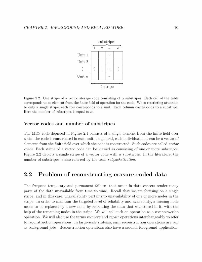
Figure 2.2: One stripe of a vector storage code consisting of ↵ substripes. Each cell of the tablecorresponds to an element from the finite field of operation for the code. When restricting attentionto only a single stripe, each row corresponds to a unit. Each column corresponds to a substripe.Here the number of substripes is equal to ↵.
Vector codes and number of substripes
The MDS code depicted in Figure 2.1 consists of a single element from the finite field overwhich the code is constructed in each unit. In general, each individual unit can be a vector ofelements from the finite field over which the code is constructed. Such codes are called vectorcodes. Each stripe of a vector code can be viewed as consisting of one or more substripes.Figure 2.2 depicts a single stripe of a vector code with ↵ substripes. In the literature, thenumber of substripes is also referred by the term subpacketization.
2.2 Problem of reconstructing erasure-coded data
The frequent temporary and permanent failures that occur in data centers render manyparts of the data unavailable from time to time. Recall that we are focusing on a singlestripe, and in this case, unavailability pertains to unavailability of one or more nodes in thestripe. In order to maintain the targeted level of reliability and availability, a missing nodeneeds to be replaced by a new node by recreating the data that was stored in it, with thehelp of the remaining nodes in the stripe. We will call such an operation as a reconstructionoperation. We will also use the terms recovery and repair operations interchangeably to referto reconstruction operations. In large-scale systems, such reconstruction operations are runas background jobs. Reconstruction operations also have a second, foreground application,

CHAPTER 2. BACKGROUND AND RELATED WORK 11
Node 1
Node 2
Node 3
Node 4
Node 5
Node 6
a1
a2
a3
a4
P4
i=1
ai
P4
i=1
iai
Figure 2.3: The traditional MDS code reconstruction framework: the first node (storing the finitefield element a
1
) is reconstructed by downloading the finite field elements from nodes 2, 3, 4 and5 (highlighted in gray) from which a
1
can be recovered. In this example, the amount of data readand transferred is k=4 times the amount of data being reconstructed.
that of degraded reads : Large-scale storage systems often receive read requests for datathat may be unavailable at that point in time. Such read requests are called degradedreads. Degraded reads are served by reconstructing the requisite data on the fly, that is, thereconstruction operation is run immediately as a foreground job.
Under replication, a reconstruction operation is carried out by copying the desired datafrom one of it replicas and creating a new replica on another node in the system. Here,the the amount of data read and transferred is equal to the amount of data being recon-structed. However, under erasure coding, there are no replicas, and hence, the part of thedata that is unavailable needs to be reconstructed through a decoding operation. Under thetraditional reconstruction framework for MDS codes, reconstruction of a node is achieved bydownloading the data stored in any k of the remaining nodes in the stripe, performing thedecoding operation, and retaining only the requisite data corresponding to the failed node.An example illustrating such a traditional reconstruction operation is depicted in Figure 2.3.In this example, data from nodes {2, 3, 4, 5} are used to reconstruct the data in node 1.
The nodes helping in a reconstruction operation are termed the helper nodes. Each helpernode transfers some data, which is in general a function of the data stored in it, to aid inthe reconstruction of the failed or otherwise unavailable node. The data from all the helpernodes is downloaded at a server and a decoding operation is performed to recover the datathat was stored on the failed or otherwise unavailable node. Thus a reconstruction operationgenerates data transfers through the interconnecting network, which consume the networkbandwidth of the cluster. The amount of data transfer involved in a reconstruction operationis also referred interchangeably by the terms reconstruction bandwidth or data download forreconstruction. A reconstruction operation also generates input-output operations at thestorage devices at the helper nodes. The amount of data that is required to be read from the

CHAPTER 2. BACKGROUND AND RELATED WORK 12
storage devices at the helper nodes is referred to as the amount of data read or data accessedor I/O. In the example depicted in Figure 2.3, nodes {2, 3, 4, 5} are the helper nodes, andthe amount of network transfer and I/O involved in the reconstruction are both four (finitefield elements). If q is the size of the finite field over which the code is constructed, thiscorresponds to log
q
(4) bits.
Thus, while traditional erasure codes provide significant increase in storage e�ciency ascompared to replication, they can result in significant increase in the amount of networktransfers and I/O during reconstruction of failed or otherwise unavailable nodes.
2.3 Related literature
In this section, we provide a high-level overview of the landscape of the related literature.More extensive discussions on the related works in relation to the contributions of this thesisare provided in the respective chapters.
Reconstruction-e�cient codes
There has been considerable amount of work in the recent past on constructing resource-e�cient codes for distributed storage.
Regenerating codes
In a seminal work [41], Dimakis et al., introduced the regenerating codes model, which opti-mizes the amount of data downloaded during repair operations. In [41], the authors providea network-flow (cutset) based lower bound for the amount of data download during what iscalled a functional repair. Under functional repair, the repaired node is only functionallyequivalent to the failed node. In [41, 182], the authors showed the theoretical existence ofcodes meeting the cutset bound for the functional repair setting. We will consider a morestringent requirement termed exact repair, wherein the reconstructed node is required to beidentical to the failed node.
The cutset bound on the repair bandwidth leads to a trade-o↵ between the storage spaceused per node and the bandwidth consumed for repair operations, and this trade-o↵ is calledthe storage-bandwidth tradeo↵ [41]. Two important points on the trade-o↵ are its endpoints termed the Minimum-Storage-Regenerating (MSR) and the Minimum-Bandwidth-Regenerating (MBR) points. MSR codes are MDS, and thus minimize the amount of storage
CHAPTER 2. BACKGROUND AND RELATED WORK 13
space consumed. For this minimal amount of storage space, MSR codes also minimize theamount of data downloaded during repair. On the other hand, MBR codes achieve the mini-mum possible download during repair while compromising on the storage space consumption.It has been shown that the MSR and MBR points are achievable even under the requirementof exact repair [127, 149, 26, 25, 115, 169]. It has also been shown that the intermediatepoints are not achievable for exact repair [149], and that there is a non-vanishing gap atthese intermediate points between the cutset bound and what is achievable [172]. Recently,there are a number of works on characterizing tighter outer bounds for the intermediatepoints [145, 46, 123, 43] and constructing codes for these points [60, 173, 45].
There have been several works on constructing explicit MSR and MBR codes [132, 127,149, 156, 164, 115, 169, 26, 185]. MSR codes are of particular interest since they areMDS. The Product-Matrix MSR codes [127] are explicit, practical MSR code constructionswhich have linear number of substripes. However, these codes have a low rate (i.e., highredundancy), requiring a storage overhead of
�2� 1
n
�or higher. In [25], the authors show
the existence of high-rate MSR codes as the number of substripes approaches infinity. TheMSR constructions presented in [115, 169, 26, 185] are high rate and have a finite numberof substripes. However, the number of substripes in these constructions is exponential ink. In fact, it has been shown that exponential number of substripes (more specificallyr
kr ) is necessary for high-rate MSR codes optimizing both the amount of data read and
downloaded [168]. In [61], the authors present a lower bound on the number of substripesfor MSR codes which optimize only for data download and do not optimize for data read.In [27, 144], MSR codes with polynomial number of substripes are presented for the settingof constant (high) rate greater than 2
3
.
Improving reconstruction e�ciency in existing codes
Binary MDS codes have received special attention in the literature due to their extensive usein disk array systems, for instance, EVEN-ODD and RDP codes [21, 35]. The EVEN-ODDand RDP codes have been optimized for reconstruction in [178] and [183] respectively. Arecent work [64] presents a reconstruction framework for traditional Reed-Solomon codes forreducing the amount of data transfer during reconstruction by downloading elements from asub-field rather than the finite field over which the code is constructed. This work optimizesonly the amount of data downloaded and not the amount of data read during reconstruction.
CHAPTER 2. BACKGROUND AND RELATED WORK 14
Computer-search based techniques
In [89], the authors present a search-based approach to find reconstruction symbols thatoptimize I/O for arbitrary binary erasure codes, but this search problem is shown to be NP-hard. The authors also present a reconstruction-e�cient MDS code construction based onRS codes, called Rotated-RS, with the number of substripes being 2. However, it supportsat most 3 parities, and moreover, its fault-tolerance capability is established via a computersearch.
Other settings
There are several other works in the literature that construct reconstruction-e�cient codesthat do not directly fall into the three areas listed above. These include codes that providesecurity [118, 148, 133, 159, 48, 138, 62, 170, 36, 83, 59, 75], co-operative reconstruction [88,157, 70, 95, 80], di↵erent cost models [153, 3], oblivious updates [106, 107], and others [126,154, 113].
Optimizing locality of reconstruction
Reconstruction-locality, that is the number of nodes contacted during a reconstruction op-eration, is another metric of interest that has been studied extensively in the recent litera-ture [110, 58, 116, 84, 114, 167, 161]. However, all the code constructions under this umbrellatrade the MDS property (that is storage e�ciency) in order to achieve a locality smaller thank.
Erasure codes in storage systems
Since decades, disk arrays have employed erasure codes to achieve space-e�cient fault-tolerance in the form of Redundant Array of Inexpensive Disks (RAID) systems [117]. Thebenefits of erasure coding over replication for providing fault tolerance in distributed storagesystems has also been well studied [191, 180], and erasure codes have been employed in manysettings such as network-attached-storage systems [2], peer-to-peer storage systems [93, 142],etc. Recently, erasure coding is being increasing deployed in datacenter-scale distributedstorage systems [51, 66, 34, 104, 181, 74] to achieve fault tolerance while minimizing storagerequirements.

15
Chapter 3
Measurements from Facebook’s datawarehouse cluster in production
In this chapter, we present our measurements from Facebook’s data warehouse clusterin production that stores hundreds of petabytes of data across a few thousand machines.We present statistics related to data unavailability in the cluster and how erasure codingimpacts resource consumption in the cluster. This study serves two purposes: (i) it providesan insight into how large-scale distributed storage systems in production are employingtraditional erasure codes, and (ii) the measurements reveal that there is a significant increasein the network tra�c due to the recovery operations of erasure-coded data, thus serving asa real-world motivation for the following chapters. To the best of our knowledge, this isthe first study in the literature that looks at the e↵ect of the reconstruction operations oferasure-coded data on the usage of network resources in data centers.
3.1 Overview of the warehouse cluster
In this section, we provide a brief description of Facebook’s data warehouse cluster in produc-tion (based on the system in production in 2013), on which we performed the measurementspresented in this chapter.
Before delving into the details of the data warehouse cluster, we will introduce someterms related to data-center architecture in general. In data centers, typically, the computingand the networking equipment are housed within racks. A rack is a group of 30-40 serversconnected to a common network switch. This switch is termed the top-of-rack (TOR) switch.

CHAPTER 3. MEASUREMENTS FROM FACEBOOK’S DATA WAREHOUSECLUSTER IN PRODUCTION 16
1"byte"block"1"
block"10"
block"11"
block"14"
256"MB"
byte2level"stripe" block2level"stripe"
…"
…"
…"
…"data"
blocks"
parity"blocks"
Figure 3.1: Erasure coding across blocks: 10 data blocks encoded using (k = 10, r = 4) RS code togenerate 4 parity blocks.
The top-of-rack switches from all the racks are interconnected through one or more layersof higher level switches (aggregation switches and routers) to provide connectivity from anyserver to any other server in the data center. Typically, the top-of-rack and higher levelswitches are heavily oversubscribed.
Facebook’s data warehouse cluster in production is a Hadoop cluster, where the storagelayer is the Hadoop Distributed File System (HDFS). The cluster comprises of two HDFSclusters, which we shall refer to as clusters A and B. In terms of the physical size, the twocluster together stores hundreds of petabytes of data, and the storage capacity used in theclusters is growing at a rate of a few petabytes every week. The cluster stores data across afew thousand machines, each of which has a storage capacity of 24-36TB. The data storedin this cluster is immutable until it is deleted, and is compressed prior to being stored in thecluster.
Since the amount of data stored is very large, the cost of operating the cluster is dom-inated by the cost of the storage capacity. The most frequently accessed data is stored as3 replicas, to allow for e�cient scheduling of the map-reduce jobs. In order to save on thestorage costs, the data which has not been accessed for more than three months is stored asa (k = 10, r = 4) Reed-Solomon (RS) code. The cluster stores more than ten petabytes ofRS-coded data. Since the employed RS code has a redundancy of only 1.4, this results inhuge savings (multiple petabytes) in storage capacity as compared to 3-way replication.
3.2 Erasure coding in the warehouse cluster
We shall now delve deeper into details of the RS-coded data in the cluster. A file or a directoryto be stored is first partitioned into blocks of size 256MB. These blocks are grouped into setsof 10 blocks each; every set is then encoded with a (k = 10, r = 4) RS code to obtain 4

CHAPTER 3. MEASUREMENTS FROM FACEBOOK’S DATA WAREHOUSECLUSTER IN PRODUCTION 17
!"#$ !"#$ !"#$ !"#$
%&'#()*+,$
!"# !$#!"#%#!$#
!"#%#$!$#
&# &# &# &#
-(.+$/$ -(.+$0$ -(.+$1$ -(.+$2$
30$
Figure 3.2: Recovery of erasure-coded data: a single missing block (a1
) is recovered by readinga block each at nodes 2 and 3 and transferring these two blocks through the top-of-rack (TOR)switches and the aggregation switch (AS).
parity blocks. As illustrated in Figure 3.1, one byte each at corresponding locations in the10 data blocks are encoded to generate the corresponding bytes in the 4 parity blocks. Theset of these 14 blocks constitutes a stripe of blocks. The 14 blocks belonging to a particularstripe are placed on 14 distinct (randomly chosen) machines. In order to secure the dataagainst rack failures, these machines are typically chosen from distinct racks.
To recover a missing or otherwise unavailable block, any 10 of the remaining 13 blocksof its stripe are read and downloaded. Since each block is placed on a di↵erent rack, thesetransfers take place through the top-of-rack switches. This consumes cross-rack bandwidththat is typically heavily oversubscribed in most data centers including the one studied here.Figure 3.2 illustrates the recovery operation through an example with (k = 2, r = 2) code.Here the first data unit a
1
(stored in server/node 1) is being recovered by downloading datafrom node 2 and node 3.
3.3 Measurements and observations
In this section, we present our measurements from the Facebook’s data warehouse clus-ter, and analyze them to study the impact of recovery of RS-coded data on the networkinfrastructure.
Unavailability statistics
We begin with some statistics on machine unavailability events. Figure 3.3 plots the numberof machines that were unavailable for more than 15 minutes in a day, over the period 22nd
January to 24th February 2013 (15 minutes is the default wait time of the cluster to flag a

CHAPTER 3. MEASUREMENTS FROM FACEBOOK’S DATA WAREHOUSECLUSTER IN PRODUCTION 18
Figure 3.3: The number of machines unavailable for more than 15 minutes in a day. The dottedline represents the median value which is 52.
machine as unavailable). We observe that the median is more than 50 machine-unavailabilityevents per day. This reasserts the necessity of redundancy in the data for both reliabilityand availability. A subset of these events ultimately trigger recovery operations.
Number of missing blocks in a stripe
Table 3.1 below shows the percentage of stripes with di↵erent number of blocks missing (onaverage). These statistics are based on data collected over a period of 6 months.
Number of missing blocks Percentage of stripes
1 98.08 %
2 1.87 %
3 0.036 %
4 9⇥ 10�4 %
>5 9⇥ 10�6 %
Table 3.1: Percentage of stripes with di↵erent numbers of missing blocks (average of data collectedover a period of six months).
We can see that one block missing in a stripe is the most dominant case: 98 % of all the

CHAPTER 3. MEASUREMENTS FROM FACEBOOK’S DATA WAREHOUSECLUSTER IN PRODUCTION 19
Figure 3.4: RS-coded HDFS blocks reconstructed and cross-rack bytes transferred for recoveryoperations per day, over a duration of around a month. The dotted lines represent the medianvalues.
stripes with missing blocks have only one block missing. Thus recovering from single failuresis by-far the most common scenario.
We now move on to measurements pertaining to the recovery operations for RS-codeddata in the cluster. The analysis below is based on the data collected from Cluster A for thefirst 24 days of February 2013.
Number of block recoveries
Figure 3.4 shows the number of block recoveries triggered each day. A median of 95, 500blocks of RS-coded data are recovered each day.
Cross-rack network transfers
We measured the number of bytes transferred across racks for the recovery of RS-codedblocks. The measurements, aggregated per day, are depicted in Figure 3.4. As shown inthe figure, a median of more than 180 TB and a maximum of 250 TB of data is transferredthrough the top-of-rack switches every day solely for the purpose of recovering RS-codeddata. The recovery operations, thus, consume a large amount of cross-rack bandwidth,thereby rendering the bandwidth unavailable for the foreground map-reduce jobs.
CHAPTER 3. MEASUREMENTS FROM FACEBOOK’S DATA WAREHOUSECLUSTER IN PRODUCTION 20
3.4 Summary
In this chapter, we presented our measurements and observations from Facebook’s datawarehouse cluster in production that stores hundreds of petabytes of data across a fewthousand machines, focusing on the unavailability statistics and the impact of using erasurecodes (in particular, RS codes) on the network infrastructure of a data center. In ourmeasurements, we observed a median of more than 50 machine unavailability events perday. These unavailablility measurements corroborate the previous reports from other datacenters regarding unavailabities being the norm rather than the exception. The analysis ofthe measurements also revealed that for the erasure-coded data, single failures in a stripe isby far the most dominant scenario. Motivated by this, we will be focusing on optimizing forreconstruction of single failure in a stripe in the following chapters. We also observed thatthe large amount of download performed by the RS-encoded data during reconstruction ofmissing blocks consumes a significantly high amount of network bandwidth and in particular,puts additional burden on the already oversubscribed top-of-rack switches. This provides areal-world motivation for our work on reconstruction-e�cient erasure codes for distributedstorage presented in the next few chapters.
21
Chapter 4
Piggybacking framework forconstructing distributed storage codes
In this chapter, we present a new framework for constructing distributed storage codes, whichwe call the Piggybacking framework, that o↵ers a rich design space for constructing storagecodes optimizing for I/O and network usage while retaining the storage e�ciency o↵ered bytraditional MDS codes. We also present three code constructions based on the Piggybackingframework that target di↵erent settings. In addition, we show how the piggybacking frame-work can be employed to enable e�cient reconstruction of the parity units in existing codesthat were originally designed to address the reconstruction of only the data units.
4.1 Introduction
A primary contributor to the cost of any large-scale storage system is the storage hardware.Further, several auxiliary costs, such as those of networking equipment, physical space, andcooling, grow proportionally with the amount of storage used. As a consequence, it is criticalfor any storage code to minimize the storage space consumed. With this motivation, we focuson codes that are MDS and have a high rate. (Recall from Chapter 2 that MDS codes areoptimal in utilizing the storage space in providing reliability, and that codes with high ratehave a small storage overhead factor.)
Further, recall from the measurements from Facebook’s data warehouse cluster in pro-duction presented in Chapter 3, that the scenario of a single node failure in a stripe is byfar the most prevalent. With this motivation, we will focus on optimizing for the case of asingle failure in a stripe.

CHAPTER 4. PIGGYBACKING FRAMEWORK FOR CONSTRUCTINGDISTRIBUTED STORAGE CODES 22
There has been considerable recent work in the area of designing reconstruction-e�cientcodes for distributed storage systems; these works are discussed in detail in Section 4.2. Ofparticular interest are the family Minimum Storage Regenerating (MSR) codes, which areMDS. While the papers [41, 182] showed the theoretical existence of MSR codes, severalrecent works [127, 156, 164, 115, 169, 26] have presented explicit MSR constructions fora wide range of parameters. Product-Matrix codes [127], and MISER codes [156, 164] areexplicit MSR code constructions which have a number of substripes linear in k. However,these codes have a low rate – MISER codes require a storage overhead of 2 and Product-Matrix codes require a storage overhead of
�2� 1
n
�. The constructions provided in [115, 169,
26] are high rate, but, necessarily require the number of substripes to be exponential in k. Infact, it has been shown in [168], that an exponential number of substripes (more specificallyr
kr ) is a fundamental limitation of any high-rate MSR code optimizing both the amount of
data read and downloaded.
The requirement of a large number of substripes presents multiple challenges on thesystems front: (i) A large number of substripes results in a large number of fragmentedreads which is detrimental to the read-latency performance of disks, (ii) A large number ofsubstripes, as a minor side e↵ect, also restricts the minimum size of files that can be handledby the code. This restricts the range of file sizes that the storage system can handle. Werefer the reader to Chapter 5 to see how the number of substripes manifests as practicalchallenges when employed in a distributed storage system. In addition to this practicalmotivation, there is also considerable theoretical interest in constructing reconstruction-e�cient codes that are MDS, high-rate and have a smaller number of substripes [27, 61,144]. To the best of our knowledge, the only explicit codes that meet these requirementsare the Rotated-RS [89] codes and the (reconstruction-optimized) EVENODD [21, 178] andRDP [35, 183] codes, all of which are MDS, high-rate and have either a constant or linear (ink) number of substripes. However, Rotated-RS codes exist only for r 2 {2, 3} and k 36,and the (reconstruction-optimized) EVENODD and RDP codes exist only for r = 2.
Furthermore, in any code, the amount of data read during a reconstruction operationis atleast as much as the amount of data downloaded, but in general, the amount of dataread can be significantly higher than the amount downloaded. This is because, many codes,including the regenerating codes, allow each node to read all its data, perform some com-putations, and transfer only the result. Our interest is in reducing both the amount of dataread and downloaded.
Here, we investigate the problem of constructing distributed storage codes that are e�-cient with respect to both the amount of data read and downloaded during reconstruction,while satisfying the constraints of (i) being MDS, (ii) having a high-rate, and (iii) having asmall (constant or linear) number of substripes. To this end, we present a new framework
CHAPTER 4. PIGGYBACKING FRAMEWORK FOR CONSTRUCTINGDISTRIBUTED STORAGE CODES 23
for constructing distributed storage codes, which we call the piggybacking framework. In anutshell, the piggybacking framework considers multiple instances of an existing code, anda piggybacking operation adds (carefully designed) functions of the data from one instanceto another.1 The framework preserves many useful properties of the underlying code suchas the minimum distance and the finite field of operation.
The piggybacking framework facilitates construction of codes that are MDS, high-rate,and have a constant (as small as 2) number of substripes, with the smallest average amount ofdata read and downloaded during reconstruction among all other known codes in this class.An appealing feature of piggyback codes is that they support all values of the code parametersk and r � 2. The typical savings in the average amount of data read and downloaded duringreconstruction is 25% to 50% depending on the choice of the code parameters. In additionto the aforementioned class of codes (which we will term as Class 1), the piggybackingframework o↵ers a rich design space for constructing codes for a wide variety of other settings.We illustrate the power of this framework by providing the following three additional classesof explicit code constructions.
(Class 2) Binary MDS codes with the lowest average amount of data read anddownloaded for reconstruction Binary MDS codes are extensively used in disk ar-rays [21, 35]. Using the piggybacking framework, we construct binary MDS codes that, tothe best of our knowledge, result in the lowest average amount of data read and downloadedfor reconstruction among all existing binary MDS codes for r � 3. Our codes support allthe parameters for which binary MDS codes are known to exist. The codes constructed herealso optimize the reconstruction of parity nodes along with that of systematic nodes.
(Class 3) MDS codes with smallest possible repair locality Repair locality is thenumber of nodes that need to be contacted during a repair operation. Several recentworks [110, 58, 116, 84, 161] present codes optimizing for repair locality. However, thesecodes are not MDS. Given our focus on MDS codes, we use the piggybacking frameworkto construct MDS codes that have the smallest possible repair locality of (k + 1) 2. To thebest of our knowledge, the amount of data read and downloaded during reconstruction inthe presented code is the smallest among all known explicit, exact-repair, minimum-locality,MDS codes for more than three parities (i.e., (n� k) > 3).
1Although we focus on MDS codes, it turns out that the piggybacking framework can be employed withnon-MDS codes as well.
2A locality of k is also possible in MDS codes, but this necessarily mandates the download of the entiredata, and hence we do not consider this option.

CHAPTER 4. PIGGYBACKING FRAMEWORK FOR CONSTRUCTINGDISTRIBUTED STORAGE CODES 24
(Class 4) A method for reducing the amount of data read and downloaded forrepair of parity nodes in existing codes that address only repair of systematicnodes The problem of e�cient node-repair in distributed storage systems has attractedconsiderable recent attention. However, many of the proposed codes [89, 26, 155, 179, 115]have algorithms for e�cient repair of only the systematic nodes. We show how the proposedpiggybacking framework can be employed to enable e�cient repair of parity nodes in suchcodes, while also retaining the e�ciency of the repair of systematic nodes.
Organization
The rest of the chapter is organized as follows. A discussion on related literature is providedin Section 4.2. Section 4.3 presents two examples that highlight the key ideas behind thePiggybacking framework. Section 4.4 introduces the general piggybacking framework. Sec-tions 4.5 and 4.6 present code designs and reconstruction algorithms based on the piggyback-ing framework, special cases of which result in classes 1 and 2 discussed above. Section 4.7provides a piggyback design which enables a small repair-locality in MDS codes (Class 3).Section 4.8 provides a comparison of Piggyback codes with various other codes in the liter-ature. Section 4.9 demonstrates the use of piggybacking to enable e�cient parity repair inexisting codes that were originally constructed for repair of only the systematic nodes (Class4).
4.2 Related work
Recall from Chapter 2 that MSR codes are MDS, and hence they are of particular relevanceto this chapter. There have been several works on constructing explicit MSR codes [127, 156,164, 26, 115, 169]. The Product-Matrix MSR codes [127] are explicit, practical MSR codeconstructions which have linear number of substripes. However, these codes have a low rate(i.e., high redundancy), requiring a storage overhead of
�2� 1
n
�or higher. In [25], the authors
show the existence of high-rate MSR codes as the number of substripes approaches infinity.The MSR constructions presented in [115, 169, 26] are high rate and have a finite numberof substripes. However, the number of substripes in these constructions is exponential ink. In fact, it has been shown that exponential number of substripes (more specificallyr
kr ) is necessary for high-rate MSR codes optimizing both the amount of data read and
downloaded [168]. In [61], the authors present a lower bound on the number of substripesfor MSR codes which optimize only for data download and do not optimize for data read.In [27, 144], MSR codes with polynomial number of substripes are presented for the setting of

CHAPTER 4. PIGGYBACKING FRAMEWORK FOR CONSTRUCTINGDISTRIBUTED STORAGE CODES 25
constant (high) rate greater than 2
3
. On the other hand, piggybacking framework allows forconstruction of repair-e�cient codes with respect to the amount of data read and downloadedthat are MDS, high-rate, and have a constant (as small as 2) number of substripes.
In [89], the authors present a search-based approach to find reconstruction symbols thatoptimize I/O for arbitrary binary erasure codes, but this search problem is shown to be NP-hard. The authors also present a reconstruction-e�cient MDS code construction based onRS codes, called Rotated-RS, with the number of substripes being 2. However, it supportsat most 3 parities, and moreover, its fault-tolerance capability is established via a computersearch. In contrast, piggybacking framework is applicable for all parameters, and piggy-backed RS codes achieve same or better savings in the amount of data read and download.
Binary MDS codes have received special attention due to their extensive use in disk arraysystems [21, 35]. The EVEN-ODD and RDP codes have been optimized for reconstructionin [178] and [183] respectively. In [47], the authors present a binary MDS code constructionfor 2 parities that achieve the regenerating codes bound for repair of systematic nodes. Incomparison, the repair-optimized binary MDS code constructions based on the Piggybackingframework provide as good or better savings for greater than 2 parities and also address therepair of both systematic and parity nodes.
Repair-locality, that is the number nodes contacted during the repair operation, is anothermetric of interest in distributed storage systems. Optimizing codes for repair-locality hasbeen extensively studied [110, 58, 116, 84, 161] in the recent past. However, all the codeconstructions under this umbrella give up on the MDS property to get smaller locality than k.
Most of the related works discussed above take the conceptual approach of constructingvector codes in order to improve the e�ciency of reconstruction with respect to the amountof data downloaded or both the amount of data read and downloaded. In a recent work [64],the authors present a reconstruction framework for (scalar) Reed-Solomon codes for reducingthe amount of data downloaded by downloading elements from a subfield rather than thefinite field over which the code is constructed. This work optimizes only the amount of datadownloaded and not the amount of data read.
4.3 Examples
We now present two examples that highlight the key ideas behind the piggybacking frame-work. The first example illustrates a method of piggybacking for reducing the amount ofdata read and downloaded during reconstruction of systematic nodes.

CHAPTER 4. PIGGYBACKING FRAMEWORK FOR CONSTRUCTINGDISTRIBUTED STORAGE CODES 26
Node 1
Node 2
Node 3
Node 4
Node 5
Node 6
An MDS Code
a1
b1
a2
b2
a3
b3
a4
b4
P4
i=1
ai
P4
i=1
bi
P4
i=1
iai
P4
i=1
ibi
(a)
Intermediate Step
a1
b1
a2
b2
a3
b3
a4
b4
P4
i=1
ai
P4
i=1
bi
P4
i=1
iai
P4
i=1
ibi
+P2
i=1
iai
(b)
Piggybacked Code
a1
b1
a2
b2
a3
b3
a4
b4
P4
i=1
ai
P4
i=1
bi
P4
i=3
iai
�P4
i=1
ibi
P4
i=1
ibi
+P2
i=1
iai
(c)
Figure 4.1: An example illustrating e�cient repair of systematic nodes using the piggybackingframework. Two instances of a (n=6,k=4) MDS code are piggybacked to obtain a new (n=6,k=4)MDS code that achieves 25% savings in the amount of data read and downloaded during the repairof any systematic node. A highlighted cell indicates a modified symbol.
Example 1. Consider two instances of a (n = 6, k = 4) MDS code as shown in Fig. 4.1a,with the 8 message symbols {a
i
}4i=1
and {bi
}4i=1
(each column of Fig. 4.1a depicts a singleinstance of the code). One can verify that the message can be recovered from the data of any4 nodes. The first step of piggybacking involves adding
P2
i=1
iai
to the second symbol of node6 as shown in Fig. 4.1b. The second step in this construction involves subtracting the secondsymbol of node 6 in the code of Fig. 4.1b from its first symbol. The resulting code is shownin Fig. 4.1c. This code has 2 substripes (the number of columns in Fig. 4.1c).
We now present the repair algorithm for the piggybacked code of Fig. 4.1c. Consider therepair of node 1. Under our repair algorithm, the symbols b
2
, b3
, b4
andP
4
i=1
bi
are downloadfrom the other nodes, and b
1
is decoded. In addition, the second symbol (P
4
i=1
ibi
+P
2
i=1
iai
)of node 6 is downloaded. Subtracting out the components of {b
i
}4i=1
gives the piggybackP2
i=1
iai
. Finally, the symbol a2
is downloaded from node 2 and subtracted to obtain a1
.Thus, node 1 is repaired by reading only 6 symbols which is 25% smaller than the total sizeof the message. Node 2 is repaired in a similar manner. Repair of nodes 3 and 4 follows onsimilar lines except that the first symbol of node 6 is read instead of the second.
The piggybacked code is MDS, and the entire message can be recovered from any 4 nodesas follows. If node 6 is one of these four nodes, then add its second symbol to its first, torecover the code of Fig. 4.1b. Now, the decoding algorithm of the original code of Fig, 4.1a isemployed to first recover {a
i
}4i=1
, which then allows for removal of the piggyback (P
2
i=1
iai
)from the second substripe, making the remainder identical to the code of Fig. 4.1c.
CHAPTER 4. PIGGYBACKING FRAMEWORK FOR CONSTRUCTINGDISTRIBUTED STORAGE CODES 27
Node 1
Node 2
Node 3
Node 4
Node 5
Node 6
a1
b1
c1
d1
a2
b2
c2
d2
a3
b3
c3
d3
a4
b4
c4
d4
P4
i=1
ai
P4
i=1
bi
P4
i=1
ci
+P4
i=1
ibi
+P2
i=1
iai
P4
i=1
di
P4
i=3
iai
�P4
i=1
ibi
P4
i=1
ibi
+P2
i=1
iai
P4
i=3
ici
�P4
i=1
idi
P4
i=1
idi
+P2
i=1
ici
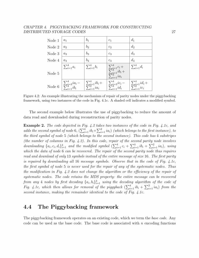
Figure 4.2: An example illustrating the mechanism of repair of parity nodes under the piggybackingframework, using two instances of the code in Fig. 4.1c. A shaded cell indicates a modified symbol.
The second example below illustrates the use of piggybacking to reduce the amount ofdata read and downloaded during reconstruction of parity nodes.
Example 2. The code depicted in Fig. 4.2 takes two instances of the code in Fig. 4.1c, andadds the second symbol of node 6, (
P4
i=1
ibi
+P
2
i=1
iai
) (which belongs to the first instance), tothe third symbol of node 5 (which belongs to the second instance). This code has 4 substripes(the number of columns in Fig. 4.2). In this code, repair of the second parity node involvesdownloading {a
i
, ci
, di
}4i=1
and the modified symbol (P
4
i=1
ci
+P
4
i=1
ibi
+P
2
i=1
iai
), usingwhich the data of node 6 can be recovered. The repair of the second parity node thus requiresread and download of only 13 symbols instead of the entire message of size 16. The first parityis repaired by downloading all 16 message symbols. Observe that in the code of Fig. 4.1c,the first symbol of node 5 is never used for the repair of any of the systematic nodes. Thusthe modification in Fig. 4.2 does not change the algorithm or the e�ciency of the repair ofsystematic nodes. The code retains the MDS property: the entire message can be recoveredfrom any 4 nodes by first decoding {a
i
, bi
}4i=1
using the decoding algorithm of the code ofFig. 4.1c, which then allows for removal of the piggyback (
P4
i=1
ibi
+P
2
i=1
iai
) from thesecond instance, making the remainder identical to the code of Fig. 4.1c.
4.4 The Piggybacking framework
The piggybacking framework operates on an existing code, which we term the base code. Anycode can be used as the base code. The base code is associated with n encoding functions
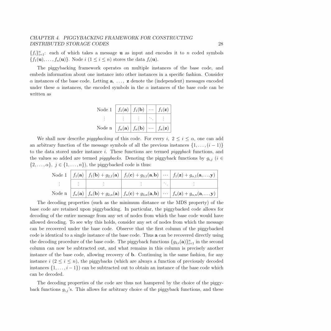
CHAPTER 4. PIGGYBACKING FRAMEWORK FOR CONSTRUCTINGDISTRIBUTED STORAGE CODES 28
{fi
}ni=1
: each of which takes a message u as input and encodes it to n coded symbols{f
1
(u), . . . , fn
(u)}. Node i (1 i n) stores the data fi
(u).
The piggybacking framework operates on multiple instances of the base code, andembeds information about one instance into other instances in a specific fashion. Consider↵ instances of the base code. Letting a, . . . , z denote the (independent) messages encodedunder these ↵ instances, the encoded symbols in the ↵ instances of the base code can bewritten as
Node 1...
Node n
f1
(a) f1
(b) · · · f1
(z)...
.... . .
...
fn
(a) fn
(b) · · · fn
(z)
We shall now describe piggybacking of this code. For every i, 2 i ↵, one can addan arbitrary function of the message symbols of all the previous instances {1, . . . , (i � 1)}to the data stored under instance i. These functions are termed piggyback functions, andthe values so added are termed piggybacks. Denoting the piggyback functions by g
i,j
(i 2{2, . . . ,↵}, j 2 {1, . . . , n}), the piggybacked code is thus:
Node 1...
Node n
f1
(a) f1
(b) + g2,1
(a) f1
(c) + g3,1
(a,b) · · · f1
(z) + g↵,1
(a, . . . ,y)...
......
. . ....
fn
(a) fn
(b) + g2,n
(a) fn
(c) + g3,n
(a,b) · · · fn
(z) + g↵,n
(a, . . . ,y)
The decoding properties (such as the minimum distance or the MDS property) of thebase code are retained upon piggybacking. In particular, the piggybacked code allows fordecoding of the entire message from any set of nodes from which the base code would haveallowed decoding. To see why this holds, consider any set of nodes from which the messagecan be recovered under the base code. Observe that the first column of the piggybackedcode is identical to a single instance of the base code. Thus a can be recovered directly usingthe decoding procedure of the base code. The piggyback functions {g
2,i
(a)}ni=1
in the secondcolumn can now be subtracted out, and what remains in this column is precisely anotherinstance of the base code, allowing recovery of b. Continuing in the same fashion, for anyinstance i (2 i n), the piggybacks (which are always a function of previously decodedinstances {1, . . . , i� 1}) can be subtracted out to obtain an instance of the base code whichcan be decoded.
The decoding properties of the code are thus not hampered by the choice of the piggy-back functions g
i,j
’s. This allows for arbitrary choice of the piggyback functions, and these

CHAPTER 4. PIGGYBACKING FRAMEWORK FOR CONSTRUCTINGDISTRIBUTED STORAGE CODES 29
functions need to be picked judiciously to achieve the desired goals (such as e�cient repair,which is the focus of this chapter).
The piggybacking procedure described above was followed in Example 1 to obtain thecode of Fig. 4.1b from that in Fig. 4.1a. Subsequently, in Example 2, this procedure wasfollowed again to obtain the code of Fig. 4.2 from that in Fig. 4.1c.
The piggybacking framework also allows any invertible transformation of the data storedin any individual node. In other words, each node of the piggybacked code (e.g., eachrow in Fig. 4.1b) can independently undergo any invertible transformation. A invertibletransformation of data within the nodes does not alter the decoding capabilities of thecode, i.e., the message can still be recovered from any set of nodes from which it couldbe recovered in the base code. This is because, the transformation can be inverted as thefirst step followed by the usual decoding procedure. In Example 1, the code of Fig. 4.1c isobtained from Fig. 4.1b via an invertible transformation of the data of node 6.
The following theorem formally proves that piggybacking does not reduce the amount ofinformation stored in any subset of nodes.
Theorem 1. Let U1
, . . . , U↵
be random variables corresponding to the messages associatedto the ↵ instances of the base code. For i 2 {1, . . . , n}, let X
i
denote the random variablecorresponding to the (encoded) data stored in node i under the base code. Let Y
i
denote the therandom variable corresponding to the (encoded) data stored in node i under the piggybackedversion of that code. Then for any subset of nodes S ✓ {1, . . . , n},
I�{Y
i
}i2S ;U1
, . . . , U↵
�� I
�{X
i
}i2S ;U1
, . . . , U↵
�. (4.1)
Proof. Let us restrict our attention to only the nodes in set S, and let |S| denote the sizeof this set. From the description of the piggybacking framework above, the data stored ininstance j (1 j ↵) under the base code is a function of U
j
. This data can be written as a|S|-length vector f(U
j
) with the elements of this vector corresponding to the data stored inthe |S| nodes in set S. On the other hand, the data stored in instance j of the piggybackedcode is of the form (f(U
j
) + gj
(U1
, . . . , Uj�1
)) for some arbitrary (vector-valued) functions
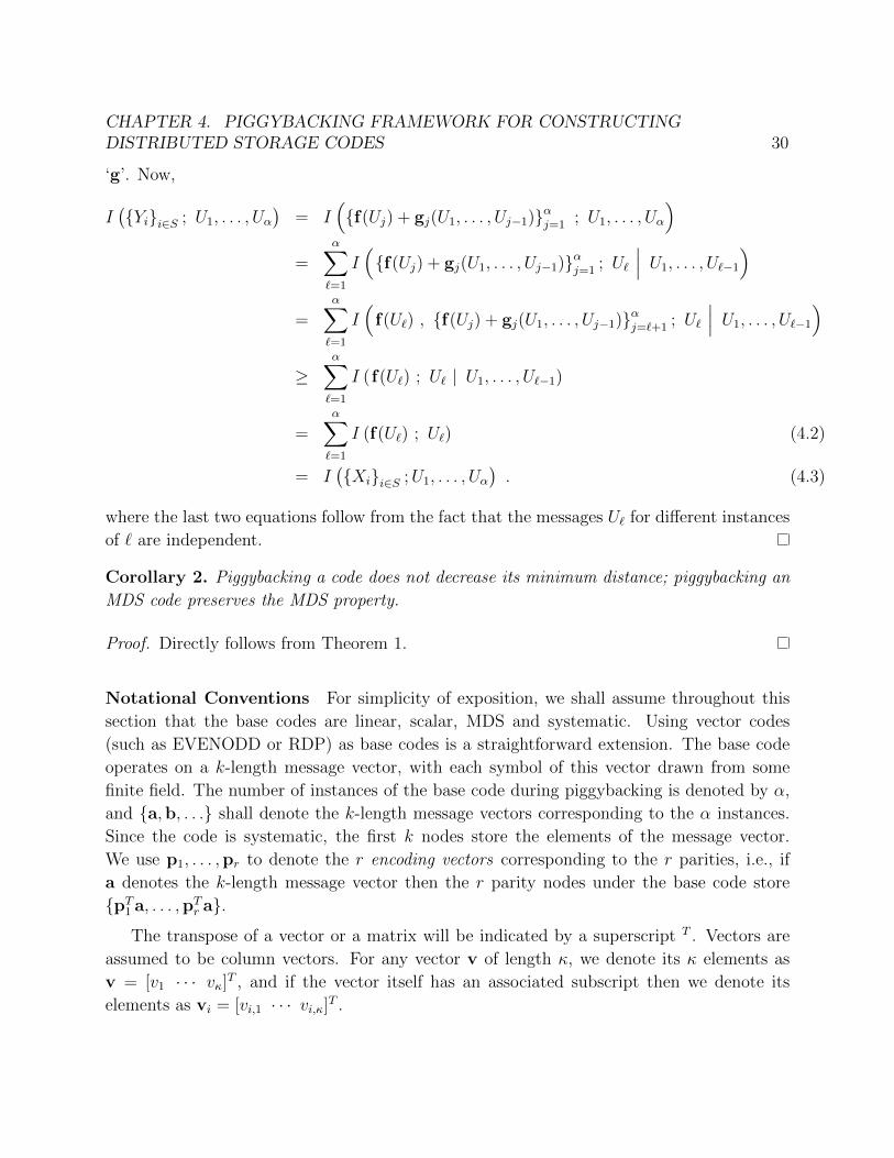
CHAPTER 4. PIGGYBACKING FRAMEWORK FOR CONSTRUCTINGDISTRIBUTED STORAGE CODES 30
‘g’. Now,
I�{Y
i
}i2S ; U
1
, . . . , U↵
�= I
⇣{f(U
j
) + gj
(U1
, . . . , Uj�1
)}↵j=1
; U1
, . . . , U↵
⌘
=↵X
`=1
I⇣{f(U
j
) + gj
(U1
, . . . , Uj�1
)}↵j=1
; U`
��� U1
, . . . , U`�1
⌘
=↵X
`=1
I⇣f(U
`
) , {f(Uj
) + gj
(U1
, . . . , Uj�1
)}↵j=`+1
; U`
��� U1
, . . . , U`�1
⌘
�↵X
`=1
I (f(U`
) ; U`
| U1
, . . . , U`�1
)
=↵X
`=1
I (f(U`
) ; U`
) (4.2)
= I�{X
i
}i2S ;U1
, . . . , U↵
�. (4.3)
where the last two equations follow from the fact that the messages U`
for di↵erent instancesof ` are independent.
Corollary 2. Piggybacking a code does not decrease its minimum distance; piggybacking anMDS code preserves the MDS property.
Proof. Directly follows from Theorem 1.
Notational Conventions For simplicity of exposition, we shall assume throughout thissection that the base codes are linear, scalar, MDS and systematic. Using vector codes(such as EVENODD or RDP) as base codes is a straightforward extension. The base codeoperates on a k-length message vector, with each symbol of this vector drawn from somefinite field. The number of instances of the base code during piggybacking is denoted by ↵,and {a,b, . . .} shall denote the k-length message vectors corresponding to the ↵ instances.Since the code is systematic, the first k nodes store the elements of the message vector.We use p
1
, . . . ,pr
to denote the r encoding vectors corresponding to the r parities, i.e., ifa denotes the k-length message vector then the r parity nodes under the base code store{pT
1
a, . . . ,pT
r
a}.
The transpose of a vector or a matrix will be indicated by a superscript T . Vectors areassumed to be column vectors. For any vector v of length , we denote its elements asv = [v
1
· · · v
]T , and if the vector itself has an associated subscript then we denote itselements as v
i
= [vi,1
· · · vi,
]T .

CHAPTER 4. PIGGYBACKING FRAMEWORK FOR CONSTRUCTINGDISTRIBUTED STORAGE CODES 31
Each of the explicit code constructions presented here possesses the property that therepair of any node entails reading of only as much data as what has to be downloaded. 3 Thisproperty is called repair-by-transfer [149]. Thus the amount of data read and the amount ofdata downloaded are equal under the presented code constructions, and hence we shall usethe same notation � to denote both these quantities.
4.5 Piggybacking design 1
In this section, we present the first design of piggyback functions and the associated repairalgorithms, which allows one to reduce the amount of data read and downloaded duringrepair while having a (small) constant number of substripes. For instance, even when thenumber of substripes is as small as 2, this piggybacking design can achieve a 25% to 50%saving in the amount of data read and downloaded during the repair of systematic nodes.We will first present the piggyback design for optimizing the repair of systematic nodes, andthen move on to the repair of parity nodes.
Repair of systematic nodes
This design operates on ↵ = 2 instances of the base code. We first partition the k systematicnodes into r sets, S
1
, . . . , Sr
, of equal size (or nearly equal size if k is not a multiple of r).For ease of understanding, let us assume that k is a multiple of r, which fixes the size ofeach of these sets to k
r
. Then, let S1
= {1, . . . , kr
}, S2
= {k
r
+ 1, . . . , 2kr
} and so on, with
Si
= { (i�1)k
r
+ 1, . . . , ikr
} for i = 1, . . . , r.
Define the k�length vectors q2
, . . . ,qr+1
,vr
to be the following projections of vector pr
:
3In general, the amount of data downloaded lower bounds the amount of data read, and the amount ofdata downloaded could be strictly smaller than that the amount of data read if a node passes a (non-injective)function of the data that it stores.

CHAPTER 4. PIGGYBACKING FRAMEWORK FOR CONSTRUCTINGDISTRIBUTED STORAGE CODES 32
q2
= [ pr,1
· · · pr,
kr
0 · · · · · · · · · · · · 0 ]T
q3
= [ 0 · · · 0 pr,
kr+1
· · · pr,
2kr
0 · · · · · · · · · 0 ]T
...
qr
= [ 0 · · · · · · · · · 0 pr,
kr (r�2)+1
· · · pr,
kr (r�1)
0 · · · 0 ]T
qr+1
= [ 0 · · · · · · · · · · · · 0 pr,
kr (r�1)+1
· · · pr,k
]T .
Also, let
vr
= pr
� qr
= [ pr,1
· · · · · · · · · pr,
kr (r�2)
0 · · · 0 pr,
kr (r�1)+1
· · · pr,k
]T .
Note that each element pi,j
is non-zero since the base code is MDS. We shall use this propertyduring repair operations.
The base code is piggybacked in the following manner:
Node 1...
Node k
Node k+1
Node k+2...
Node k+r
a1
b1
......
ak
bk
pT
1
a pT
1
b
pT
2
a pT
2
b+ qT
2
a...
...
pT
r
a pT
r
b+ qT
r
a
Fig. 4.1b depicts an example of such a piggybacking.
We shall now perform an invertible transformation of the data stored in node (k+ r). Inparticular, the first symbol of node (k + r) in the code above is replaced with the di↵erenceof this symbol from its second symbol, i.e., node (k + r) now stores
Node k+r vT
r
a� pT
r
b pT
r
b+ qT
r
a
The other symbols in the code remain intact. This completes the description of theencoding process.
Next, we present the algorithm for repair of any systematic node ` (2 {1, . . . , k}). Thisentails recovery of the two symbols a
`
and b`
from the remaining nodes.

CHAPTER 4. PIGGYBACKING FRAMEWORK FOR CONSTRUCTINGDISTRIBUTED STORAGE CODES 33
Case 1 (` /2 Sr
): Without loss of generality let ` 2 S1
. The k symbols{b
1
, . . . , b`�1
, b`+1
, . . . , bk
, pT
1
b} are downloaded from the remaining nodes, and the entirevector b is decoded (using the MDS property of the base code). It now remains to recovera`
. Observe that the `th element of q2
is non-zero. The symbol (pT
2
b+ qT
2
a) is downloadedfrom node (k+2), and since b is completely known, pT
2
b is subtracted from the downloadedsymbol to obtain the piggyback qT
2
a. The symbols {ai
}i2S1\{`} are also downloaded from the
other systematic nodes in set S1
. The specific (sparse) structure of q2
allows for recoveringa`
from these downloaded symbols. Thus the total amount of data read and downloadedduring the repair of node ` is (k + k
r
) (in comparison, the size of the message is 2k).
Case 2 (S = Sr
): As in the previous case, b is completely decoded by downloading{b
1
, . . . , b`�1
, b`+1
, . . . , bk
, pT
1
b}. The first symbol (vT
r
a�pT
r
b) of node (k+r) is downloaded.The second symbols {pT
i
b + qT
i
a}i2{2,...,r�1} of the parities (k + 2), . . . , (k + r � 1) are also
downloaded, and are then subtracted from the first symbol of node (k + r). This gives(qT
r+1
a+wTb) for some vector w. Using the previously decoded value of b, vTb is removedto obtain qT
r+1
a. Observe that the `th element of qr+1
is non-zero. The desired symbola`
can thus be recovered by downloading {a kr (r�1)+1
, . . . , a`�1
, a`+1
, . . . , ak
} from the othersystematic nodes in S
r
. Thus the total amount of data read and downloaded for recoveringnode ` is (k + k
r
+ r � 2).
Observe that the repair of systematic nodes in the last set Sr
requires larger amount ofdata to be read and downloaded as compared to the repair of systematic nodes in the othersets. Given this observation, we do not choose the sizes of the sets to be equal (as describedpreviously), and instead optimize the sizes to minimize the average read and downloadrequired. For i = 1, . . . , r, denoting the size of the set S
i
by ti
, the optimal sizes of the setsturn out to be
t1
= · · · = tr�1
=
⇠k
r+
r � 2
2r
⇡:= t, (4.4)
tr
= k � (r � 1)t . (4.5)
The amount of data read and downloaded for repair of any systematic node in the first (r�1)sets is (k + t), and the last set is (k + t
r
+ r � 2). Thus, the average amount of data readand downloaded �sys
1
for repair of systematic nodes, as a fraction of the total number 2k ofmessage symbols, is
�sys
1
=1
2k2
[(k � tr
) (k + t) + tr
(k + tr
+ r � 2)] . (4.6)
This quantity is plotted in Fig. 4.5a for several values of the system parameters n and k.

CHAPTER 4. PIGGYBACKING FRAMEWORK FOR CONSTRUCTINGDISTRIBUTED STORAGE CODES 34
Repair of parity nodes
We shall now piggyback the code constructed in Section 4.5 to introduce e�ciency in therepair of parity nodes, while also retaining the e�ciency in the repair of systematic nodes.Observe that in the code of Section 4.5, the first symbol of node (k + 1) is never read forrepair of any systematic node. We shall add piggybacks to this unused parity symbol to aidin the repair of other parity nodes.
This design employs m instances of the piggybacked code of Section 4.5. The number ofsubstripes in the resultant code is thus 2m. The choice of m can be arbitrary, and highervalues of m result in greater repair-e�ciency. For every even substripe i 2 {2, 4, . . . , 2m�2},the (r�1) parity symbols in nodes (k+2) to (k+ r) are summed up, and the result is addedas a piggyback to the (i + 1)th symbol of node (k + 1). The resulting code, when m = 2, isshown below.
Node 1...
Node k
Node k+1
Node k+2...
Node k+r-1
Node k+r
a1
b1
c1
d1
......
......
ak
bk
ck
dk
pT
1
a pT
1
b pT
1
c+P
r
i=2
(pT
i
b+ qT
i
a) pT
1
d
pT
2
a pT
2
b+ qT
2
a pT
2
c pT
2
d+ qT
2
c...
......
...
pT
r�1a pT
r�1b+ qT
r�1a pT
r�1c pT
r�1d+ qT
r�1c
vT
r
a� pT
r
b pT
r
b+ qT
r
a vT
r
c� pT
r
d pT
r
d+ qT
r
c
This completes the encoding procedure. The code of Fig. 4.2 is an example of this design.
As shown in Section 4.4, the piggybacked code retains the MDS property of the basecode. In addition, the repair of systematic nodes is identical to the that in the code ofSection 4.5, since the symbol modified in this piggybacking was never read for the repair ofany systematic node in the code of Section 4.5.
We now present an algorithm for e�cient repair of parity nodes under this piggybackdesign. The first parity node is repaired by downloading all 2mk message symbols from thesystematic nodes. Consider repair of any other parity node, say node ` 2 {k+2, . . . , k+ r}.All message symbols a, c, . . . in the odd substripes are downloaded from the systematicnodes. All message symbols of the last substripe (e.g., message d in the m = 2 code shownabove) are also downloaded from the systematic nodes. Further, the {3rd, 5th, . . . , (2m�1)th}

CHAPTER 4. PIGGYBACKING FRAMEWORK FOR CONSTRUCTINGDISTRIBUTED STORAGE CODES 35
symbols of node (k + 1) (i.e., the symbols that we modified in the piggybacking operationabove) are also downloaded, and the components corresponding to the already downloadedmessage symbols are subtracted out. By construction, what remains in the symbol fromsubstripe i (2 {3, 5, . . . , 2m � 1}) is the piggyback. This piggyback is a sum of the paritysymbols of the substripe (i � 1) from the last (r � 1) nodes (including the failed node).The remaining (r� 2) parity symbols belonging to each of the substripes {2, 4, . . . , 2m� 2}are downloaded and subtracted out, to recover the data of the failed node. The proceduredescribed above is illustrated via the repair of node 6 in Example 2.
The average amount of data read and downloaded �par
1
for repair of parity nodes, as afraction of the total message symbols, is
�par
1
=1
2kr
2k + (r � 1)
✓✓1 +
1
m
◆k +
✓1� 1
m
◆(r � 1)
◆�.
This quantity is plotted in Fig. 4.5b for several values of the system parameters n and k
with m = 4.
4.6 Piggybacking design 2
The design presented in this section provides a higher e�ciency of repair as compared to theprevious design. On the downside, it requires a larger number of substripes: the minimumnumber of substripes required under the design of Section 4.5 is 2 and under that of Sec-tion 4.5 is 4, while that required in the design of this section is (2r � 3). We first illustratethis piggybacking design with an example.
Example 3. Consider some (n = 13, k = 10) MDS code as the base code, and consider↵ = (2r � 3) = 3 instances of this code. Divide the systematic nodes into two sets of sizes 5each as S
1
= {1, . . . , 5} and S2
= {6, . . . , 10}. Define 10-length vectors q2
, v2
, q3
and v3
as
q2
= [p2,1
· · · p2,5
0 · · · 0]
v2
= [0 · · · 0 p2,6
· · · p2,10
]
q3
= [0 · · · 0 p3,6
· · · p3,10
]
v3
= [p3,1
· · · p3,5
0 · · · 0]
Now piggyback the base code in the following manner
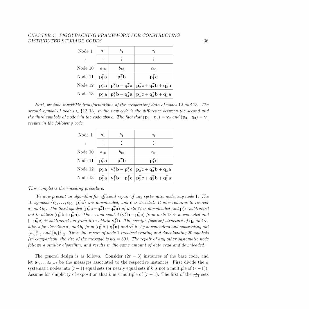
CHAPTER 4. PIGGYBACKING FRAMEWORK FOR CONSTRUCTINGDISTRIBUTED STORAGE CODES 36
Node 1...
Node 10
Node 11
Node 12
Node 13
a1
b1
c1
......
...
a10
b10
c10
pT
1
a pT
1
b pT
1
c
pT
2
a pT
2
b+ qT
2
a pT
2
c+ qT
2
b+ qT
2
a
pT
3
a pT
3
b+ qT
3
a pT
3
c+ qT
3
b+ qT
3
a
Next, we take invertible transformations of the (respective) data of nodes 12 and 13. Thesecond symbol of node i 2 {12, 13} in the new code is the di↵erence between the second andthe third symbols of node i in the code above. The fact that (p
2
�q2
) = v2
and (p3
�q3
) = v3
results in the following code
Node 1...
Node 10
Node 11
Node 12
Node 13
a1
b1
c1
......
...
a10
b10
c10
pT
1
a pT
1
b pT
1
c
pT
2
a vT
2
b� pT
2
c pT
2
c+ qT
2
b+ qT
2
a
pT
3
a vT
3
b� pT
3
c pT
3
c+ qT
3
b+ qT
3
a
This completes the encoding procedure.
We now present an algorithm for e�cient repair of any systematic node, say node 1. The10 symbols {c
2
, . . . , c10
, pT
1
c} are downloaded, and c is decoded. It now remains to recovera1
and b1
. The third symbol (pT
2
c+qT
2
b+qT
2
a) of node 12 is downloaded and pT
2
c subtractedout to obtain (qT
2
b+qT
2
a). The second symbol (vT
3
b�pT
3
c) from node 13 is downloaded and(�pT
3
c) is subtracted out from it to obtain vT
3
b. The specific (sparse) structure of q2
and v3
allows for decoding a1
and b1
from (qT
2
b+qT
2
a) and vT
3
b, by downloading and subtracting out{a
i
}5i=2
and {bi
}5i=2
. Thus, the repair of node 1 involved reading and downloading 20 symbols(in comparison, the size of the message is k↵ = 30). The repair of any other systematic nodefollows a similar algorithm, and results in the same amount of data read and downloaded.
The general design is as follows. Consider (2r � 3) instances of the base code, andlet a
1
, . . . a2r�3
be the messages associated to the respective instances. First divide the k
systematic nodes into (r�1) equal sets (or nearly equal sets if k is not a multiple of (r�1)).Assume for simplicity of exposition that k is a multiple of (r � 1). The first of the k
r�1
sets

CHAPTER 4. PIGGYBACKING FRAMEWORK FOR CONSTRUCTINGDISTRIBUTED STORAGE CODES 37
consist of the first k
r�1
nodes, the next set consists of the next k
r�1
nodes and so on. Definek-length vectors {v
i
, vi
}ri=2
as
vi
= ar�1
+ iar�2
+ i2ar�3
+ · · ·+ ir�2a1
vi
= vi
� ar�1
= iar�2
+ i2ar�3
+ · · ·+ ir�2a1
.
Further, define k-length vectors {qi,j
}r,r�1
i=2,j=1
as
qi,j
=
2
666666664
0. . .
01. . .
10. . .
0
3
777777775
pi
where the positions of the ones on the diagonal of the (k ⇥ k) diagonal matrix depictedcorrespond to the nodes in the jth group. It follows that
r�1X
j=1
qi,j
= pi
8 i 2 {2, . . . r} .
Parity node (k + i), i 2 {2, . . . , r}, is then piggybacked to store
pT
i
a1
··· pT
i
ar�2
pT
i
ar�1
+Pr�1
j=1,j 6=i�1
qT
i,j
vi
pT
i
ar
+qT
i,1
vi
··· pT
i
ar+i�3
+qT
i,i�2
vi
pT
i
ar
+qT
i,i
vi
··· pT
i
a2r�3
+qT
i,r�1
vi
Following this, an invertible linear combination is performed at each of the nodes{k + 2, . . . , k + r}. The transform subtracts the last (r � 2) substripes from the (r � 1)th
substripe, following which the node (k + i), i 2 {2, . . . , r}, stores
pT
i
a1
··· pT
i
ar�2
qT
i,i�1
ar�1
�P2r�3
j=r
pT
i
aj
pT
i
ar
+qT
i,1
vi
··· pT
i
ar+i�3
+qT
i,i�2
vi
pT
i
ar
+qT
i,i
vi
··· pT
i
a2r�3
+qT
i,r�1
vi
Let us now see how repair of a systematic node is performed. Consider repair of node `.First, from nodes {1, . . . , k+1}\{`}, all the data in the last (r�2) substripes is downloadedand the data a
r
, . . . , a2r�3
is recovered. This also provides us with a part of the desired data{a
r,`
, . . . , a2r�3,`
}. Next, observe that in each parity node {k+2, . . . , k+r}, there is preciselyone symbol whose ‘q’ vector has a non-zero `th component. From each of these nodes, thesymbol having this vector is downloaded, and the components along {a
r
, . . . , a2r�3
} are
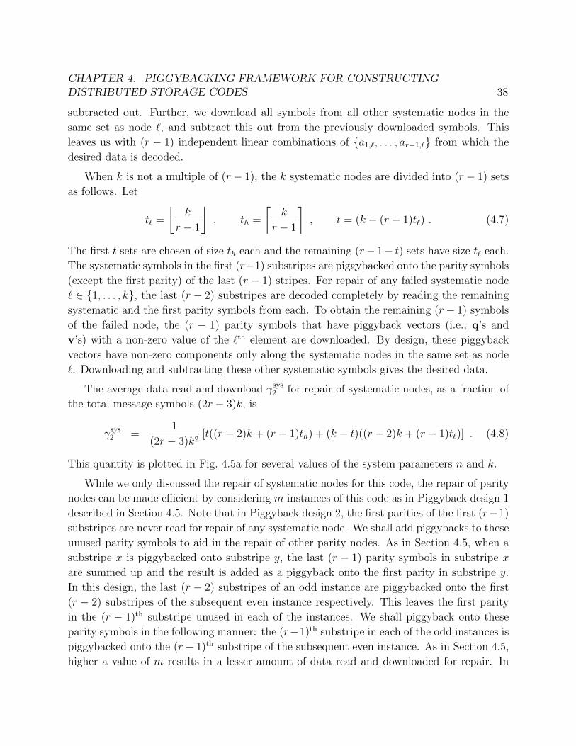
CHAPTER 4. PIGGYBACKING FRAMEWORK FOR CONSTRUCTINGDISTRIBUTED STORAGE CODES 38
subtracted out. Further, we download all symbols from all other systematic nodes in thesame set as node `, and subtract this out from the previously downloaded symbols. Thisleaves us with (r � 1) independent linear combinations of {a
1,`
, . . . , ar�1,`
} from which thedesired data is decoded.
When k is not a multiple of (r � 1), the k systematic nodes are divided into (r � 1) setsas follows. Let
t`
=
�k
r � 1
⌫, t
h
=
⇠k
r � 1
⇡, t = (k � (r � 1)t
`
) . (4.7)
The first t sets are chosen of size th
each and the remaining (r� 1� t) sets have size t`
each.The systematic symbols in the first (r�1) substripes are piggybacked onto the parity symbols(except the first parity) of the last (r � 1) stripes. For repair of any failed systematic node` 2 {1, . . . , k}, the last (r � 2) substripes are decoded completely by reading the remainingsystematic and the first parity symbols from each. To obtain the remaining (r� 1) symbolsof the failed node, the (r � 1) parity symbols that have piggyback vectors (i.e., q’s andv’s) with a non-zero value of the `th element are downloaded. By design, these piggybackvectors have non-zero components only along the systematic nodes in the same set as node`. Downloading and subtracting these other systematic symbols gives the desired data.
The average data read and download �sys
2
for repair of systematic nodes, as a fraction ofthe total message symbols (2r � 3)k, is
�sys
2
=1
(2r � 3)k2
[t((r � 2)k + (r � 1)th
) + (k � t)((r � 2)k + (r � 1)t`
)] . (4.8)
This quantity is plotted in Fig. 4.5a for several values of the system parameters n and k.
While we only discussed the repair of systematic nodes for this code, the repair of paritynodes can be made e�cient by considering m instances of this code as in Piggyback design 1described in Section 4.5. Note that in Piggyback design 2, the first parities of the first (r�1)substripes are never read for repair of any systematic node. We shall add piggybacks to theseunused parity symbols to aid in the repair of other parity nodes. As in Section 4.5, when asubstripe x is piggybacked onto substripe y, the last (r � 1) parity symbols in substripe x
are summed up and the result is added as a piggyback onto the first parity in substripe y.In this design, the last (r � 2) substripes of an odd instance are piggybacked onto the first(r � 2) substripes of the subsequent even instance respectively. This leaves the first parityin the (r � 1)th substripe unused in each of the instances. We shall piggyback onto theseparity symbols in the following manner: the (r�1)th substripe in each of the odd instances ispiggybacked onto the (r� 1)th substripe of the subsequent even instance. As in Section 4.5,higher a value of m results in a lesser amount of data read and downloaded for repair. In

CHAPTER 4. PIGGYBACKING FRAMEWORK FOR CONSTRUCTINGDISTRIBUTED STORAGE CODES 39
such a design, the average data read �par
2
for repair of parity nodes, as a fraction of the totalmessage symbols, is
�par
2
=1
r+
r � 1
(2r � 3)kmr
h(m+ 1)(r � 2)k + (m� 1)(r � 2)(r � 1) +
lm2
mk +
jm2
k(r � 1)
i.
(4.9)This quantity is also plotted in Fig. 4.5b for various values of the system parameters n andk with m = 4.
4.7 Piggybacking design 3
In this section, we present a piggybacking design to construct MDS codes with a primaryfocus on the locality of repair. The locality of a repair operation is defined as the numberof nodes that are contacted during the repair operation. The codes presented here performe�cient repair of any of the systematic nodes with the smallest possible locality for anyMDS code, which is equal to (k + 1). 4 To the best of our knowledge, the amount of dataread and downloaded during reconstruction in the presented code is the smallest among allknown explicit, exact-repair, minimum-locality, MDS codes for more than three parities (i.e.,(r > 3).
This design involves two levels of piggybacking, and these are illustrated in the followingtwo example constructions. The first example considers ↵ = 2m instances of the base codeand shows the first level of piggybacking, for any positive integerm > 1 (as we will see, highervalues of m will result in repair with a smaller amount of data read and download). Thesecond example uses two instances of this code and adds the second level of piggybacking.We note that this design deals with the repair of only the systematic nodes.
Example 4. Consider any (n = 11, k = 8) MDS code as the base code, and take 4 instancesof this code. Divide the systematic nodes into two sets as follows, S
1
= {1, 2, 3, 4}, S2
={5, 6, 7, 8}. We then add the piggybacks as shown in Fig. 4.3. Observe that in this design,the piggybacks added to an even substripe is a function of symbols in its immediately previous(odd) substripe from only the systematic nodes in the first set S
1
, while the piggybacks addedto an odd substripe are functions of symbols in its immediately previous (even) substripe fromonly the systematic nodes in the second set S
2
.
4A locality of k is also possible, but this necessarily mandates the download of the entire data, and hencewe do not consider this option.

CHAPTER 4. PIGGYBACKING FRAMEWORK FOR CONSTRUCTINGDISTRIBUTED STORAGE CODES 40
Node 1...
Node 4
Node 5...
Node 8
Node 9
Node 10
Node 11
a1
b1
c1
d1
......
......
a4
b4
c4
d4
a5
b5
c5
d5
......
......
a8
b8
c8
d8
pT
1
a pT
1
b pT
1
c pT
1
d
pT
2
a pT
2
b+a1
+ a2
pT
2
c+b5
+ b6
pT
2
d+c1
+ c2
pT
3
a pT
3
b+a3
+ a4
pT
3
c+b7
+ b8
pT
3
d+c3
+ c4
Figure 4.3: Example illustrating first level of piggybacking in design 3. The piggybacks in the evensubstripes (in blue) are a function of only the systematic nodes {1, . . . , 4} (also in blue), and thepiggybacks in odd substripes (in green) are a function of only the systematic nodes {5, . . . , 8} (alsoin green). This code requires an average amount of data read and download of only 71% of themessage size for repair of systematic nodes.
We now present the algorithm for repair of any systematic node. First consider therepair of any systematic node ` 2 {1, . . . , 4} in the first set. For instance, say ` = 1, then{b
2
, . . . , b8
, pT
1
b} and {d2
, . . . , d8
, pT
1
d} are downloaded, and {b, d} (i.e., the messages inthe even substripes) are decoded. It now remains to recover the symbols a
1
and c1
(belongingto the odd substripes). The second symbol (pT
2
b + a1
+ a2
) from node 10 is downloadedand pT
2
b subtracted out to obtain the piggyback (a1
+ a2
). Now a1
can be recovered bydownloading and subtracting out a
2
. The fourth symbol from node 10, (pT
2
d + c1
+ c2
), isalso downloaded and pT
2
d subtracted out to obtain the piggyback (c1
+ c2
). Finally, c1
isrecovered by downloading and subtracting out c
2
. Thus, node 1 is repaired by reading a totalof 20 symbols (in comparison, the total total message size is 32) and with a locality of 9. Therepair of node 2 can be carried out in an identical manner. The two other nodes in the firstset, nodes 3 and 4, can be repaired in a similar manner by reading the second and fourthsymbols of node 11 which have their piggybacks. Thus, repair of any node in the first grouprequires reading and downloading a total of 20 symbols and with a locality of 9.
Now we consider the repair of any node ` 2 {5, . . . , 8} in the second set S2
. For in-stance, consider ` = 5. The symbols
�a1
, . . . , a8
, pT
1
a \{a
5
},�c1
, . . . , c8
, pT
1
c \{c
5
} and�d1
, . . . , d8
, pT
1
d \{d
5
} are downloaded in order to decode a5
, c5
, and d5
. From node 10,the symbol (pT
2
c + b5
+ b6
) is downloaded and pT
2
c is subtracted out. Then, b5
is recovered
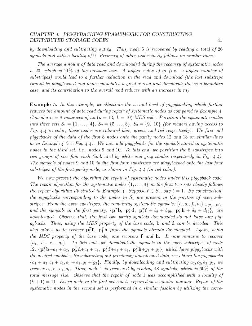
CHAPTER 4. PIGGYBACKING FRAMEWORK FOR CONSTRUCTINGDISTRIBUTED STORAGE CODES 41
by downloading and subtracting out b6
. Thus, node 5 is recovered by reading a total of 26symbols and with a locality of 9. Recovery of other nodes in S
2
follows on similar lines.
The average amount of data read and downloaded during the recovery of systematic nodesis 23, which is 71% of the message size. A higher value of m (i.e., a higher number ofsubstripes) would lead to a further reduction in the read and download (the last substripecannot be piggybacked and hence mandates a greater read and download; this is a boundarycase, and its contribution to the overall read reduces with an increase in m).
Example 5. In this example, we illustrate the second level of piggybacking which furtherreduces the amount of data read during repair of systematic nodes as compared to Example 4.Consider ↵ = 8 instances of an (n = 13, k = 10) MDS code. Partition the systematic nodesinto three sets S
1
= {1, . . . , 4}, S2
= {5, . . . , 8}, S3
= {9, 10} (for readers having access toFig. 4.4 in color, these nodes are coloured blue, green, and red respectively). We first addpiggybacks of the data of the first 8 nodes onto the parity nodes 12 and 13 on similar linesas in Example 4 (see Fig. 4.4). We now add piggybacks for the symbols stored in systematicnodes in the third set, i.e., nodes 9 and 10. To this end, we parititon the 8 substripes intotwo groups of size four each (indicated by white and gray shades respectively in Fig. 4.4).The symbols of nodes 9 and 10 in the first four substripes are piggybacked onto the last foursubstripes of the first parity node, as shown in Fig. 4.4 (in red color).
We now present the algorithm for repair of systematic nodes under this piggyback code.The repair algorithm for the systematic nodes {1, . . . , 8} in the first two sets closely followsthe repair algorithm illustrated in Example 4. Suppose ` 2 S
1
, say ` = 1. By construction,the piggybacks corresponding to the nodes in S
1
are present in the parities of even sub-stripes. From the even substripes, the remaining systematic symbols, {b
i
, di
, fi
, hi
}i={2,...,10},
and the symbols in the first parity, {pT
1
b, pT
1
d, pT
1
f + b9
+ b10
, pT
1
h + d9
+ d10
}, aredownloaded. Observe that, the first two parity symbols downloaded do not have any pig-gybacks. Thus, using the MDS property of the base code, b and d can be decoded. Thisalso allows us to recover pT
1
f , pT
1
h from the symbols already downloaded. Again, usingthe MDS property of the base code, one recovers f and h. It now remains to recover{a
1
, c1
, e1
, g1
}. To this end, we download the symbols in the even substripes of node12, {pT
2
b+a1
+ a2
, pT
2
d+c1
+ c2
, pT
2
f+e1
+ e2
, pT
2
h+g1
+ g2
}, which have piggybacks withthe desired symbols. By subtracting out previously downloaded data, we obtain the piggybacks{a
1
+ a2
, c1
+ c2
, e1
+ e2
, g1
+ g2
}. Finally, by downloading and subtracting a2
, c2
, e2
, g2
, werecover a
1
, c1
, e1
, g1
. Thus, node 1 is recovered by reading 48 symbols, which is 60% of thetotal message size. Observe that the repair of node 1 was accomplished with a locality of(k + 1) = 11. Every node in the first set can be repaired in a similar manner. Repair of thesystematic nodes in the second set is performed in a similar fashion by utilizing the corre-

CHAPTER 4. PIGGYBACKING FRAMEWORK FOR CONSTRUCTINGDISTRIBUTED STORAGE CODES 42
Node 1...
Node 4
Node 5...
Node 8
Node 9
Node 10
Node 11
Node 12
Node 13
a1
b1
c1
d1
e1
f1
g1
h1
......
......
......
......
a4
b4
c4
d4
e4
f4
g4
h4
a5
b5
c5
d5
e5
f5
g5
h5
......
......
......
......
a8
b8
c8
d8
e8
f8
g8
h8
a9
b9
c9
d9
e9
f9
g9
h9
a10
b10
c10
d10
e10
f10
g10
h10
pT
1
a pT
1
b pT
1
c pT
1
d pT
1
e+a9
+ a10
pT
1
f +b9
+ b10
pT
1
g +c9
+ c10
pT
1
h+c9
+ c10
pT
2
a pT
2
b+a1
+ a2
pT
2
c+b5
+ b6
pT
2
d+c1
+ c2
pT
2
e pT
2
f +e1
+ e2
pT
2
g +f5
+ f6
pT
2
h+g1
+ g2
pT
3
a pT
3
b+a3
+ a4
pT
3
c+b7
+ b8
pT
3
d+c3
+ c4
pT
3
e pT
3
f +e3
+ e4
pT
3
g +f7
+ f8
pT
3
h+g3
+ g4
Figure 4.4: An example illustrating piggyback design 3, with k = 10, n = 13, ↵ = 8. Thepiggybacks in the first parity node (in red) are functions of the data of nodes {8, 9} alone. Inthe remaining parity nodes, the piggybacks in the even substripes (in blue) are functions of thedata of nodes {1, . . . , 4} (also in blue), and the piggybacks in the odd substripes (in green) arefunctions of the data of nodes {5, . . . , 8} (also in green), and the piggybacks in red (also in red).The piggybacks in nodes 12 and 13 are identical to that in Example 4 (Fig 4.3). The piggybacks innode 11 piggyback the first set of 4 substripes (white background) onto the second set of numberof substripes (gray background)
.
sponding piggybacks, however, the total number of symbols read is 64 (since the last substripecannot be piggybacked; such was the case in Example 4 as well).
We now present the repair algorithm for systematic nodes {9, 10} in the third set S3
.Let us suppose ` = 9. Observe that the piggybacks corresponding to node 9 fall in thesecond group (i.e., the last four) of substripes. From the last four substripes, the remainingsystematic symbols {e
i
, fi
, gi
, hi
}i={1,...,8,10}, and the symbols in the second parity {pT
1
e, pT
1
f+e1
+ e2
, pT
1
g+ f1
+ f2
, pT
1
h+ g1
+ g2
, } are downloaded. Using the MDS property of the basecode, one recovers e, f , g and h. It now remains to recover a
9
, b9
, c9
and d9
. To this end,we download {pT
1
e + a9
+ a10
, pT
1
f + b9
+ b10
, pT
1
g + c9
+ c10
, pT
1
h + d9
+ d10
} from node11. Subtracting out the previously downloaded data, we obtain the piggybacks {a
9
+ a10
, b9
+b10
, c9
+ c10
, d9
+ d10
}. Finally, by downloading and subtracting out {a10
, b10
, c10
, d10
}, we
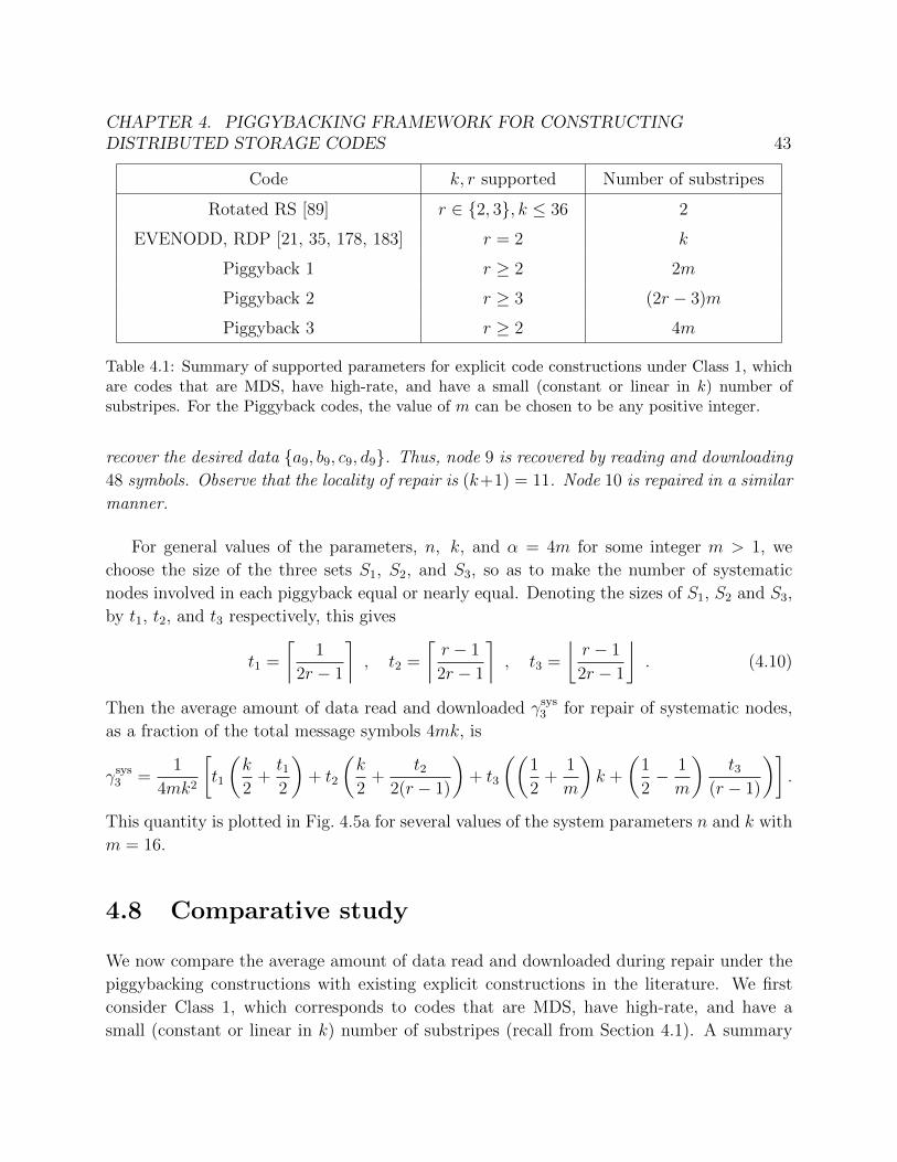
CHAPTER 4. PIGGYBACKING FRAMEWORK FOR CONSTRUCTINGDISTRIBUTED STORAGE CODES 43
Code k, r supported Number of substripes
Rotated RS [89] r 2 {2, 3}, k 36 2
EVENODD, RDP [21, 35, 178, 183] r = 2 k
Piggyback 1 r � 2 2m
Piggyback 2 r � 3 (2r � 3)m
Piggyback 3 r � 2 4m
Table 4.1: Summary of supported parameters for explicit code constructions under Class 1, whichare codes that are MDS, have high-rate, and have a small (constant or linear in k) number ofsubstripes. For the Piggyback codes, the value of m can be chosen to be any positive integer.
recover the desired data {a9
, b9
, c9
, d9
}. Thus, node 9 is recovered by reading and downloading48 symbols. Observe that the locality of repair is (k+1) = 11. Node 10 is repaired in a similarmanner.
For general values of the parameters, n, k, and ↵ = 4m for some integer m > 1, wechoose the size of the three sets S
1
, S2
, and S3
, so as to make the number of systematicnodes involved in each piggyback equal or nearly equal. Denoting the sizes of S
1
, S2
and S3
,by t
1
, t2
, and t3
respectively, this gives
t1
=
⇠1
2r � 1
⇡, t
2
=
⇠r � 1
2r � 1
⇡, t
3
=
�r � 1
2r � 1
⌫. (4.10)
Then the average amount of data read and downloaded �sys
3
for repair of systematic nodes,as a fraction of the total message symbols 4mk, is
�sys
3
=1
4mk2
t1
✓k
2+
t1
2
◆+ t
2
✓k
2+
t2
2(r � 1)
◆+ t
3
✓✓1
2+
1
m
◆k +
✓1
2� 1
m
◆t3
(r � 1)
◆�.
This quantity is plotted in Fig. 4.5a for several values of the system parameters n and k withm = 16.
4.8 Comparative study
We now compare the average amount of data read and downloaded during repair under thepiggybacking constructions with existing explicit constructions in the literature. We firstconsider Class 1, which corresponds to codes that are MDS, have high-rate, and have asmall (constant or linear in k) number of substripes (recall from Section 4.1). A summary

CHAPTER 4. PIGGYBACKING FRAMEWORK FOR CONSTRUCTINGDISTRIBUTED STORAGE CODES 44
of the supported parameters of various existing explicit constructions for Class 1 and thepiggybacking constructions is provided in Table 4.1. Fig. 4.5 presents plots comparing theamount of data read and downloaded during repair under these codes. Each of the codescompared in Fig. 4.5 have the property of repair-by-transfer [149], i.e., they read only thosesymbols that they wish to download. Consequently, the amount of data read and downloadedare equal under these codes. The average amount of data read and downloaded duringreconstruction of systematic nodes is compared in Fig. 4.5a, that during reconstruction ofparity nodes in Fig. 4.5b, and the average taking all nodes into account is compared inFig. 4.5c. Although the goal of Piggyback design 3 is to minimize the repair locality, it alsoreduces the amount of data read and downloaded during repair and hence we include it inthese comparison plots. In the plots, we consider the following number of substripes: 8 forPiggyback 1 and Rotated-RS codes, 4(2r� 3) for Piggyback 2, and 16 for Piggyback 3. Thenumber of substripes for EVENODD and RDP codes are (k � 1) and k respectively. Notethat the (repair-optimized) EVENODD and RDP codes exist only for r = 2, and Rotated-RS codes exist only for r = 3. The amount of data read and downloaded for repair underthe (repair-optimized) EVENODD and RDP codes is identical to that of a Rotated-RS codewith the same parameters.
To address Class 2, which corresponds to binary MDS codes, we propose using Piggy-backing designs 1 and 2 with traditional binary MDS array codes as the underlying basecodes (for instance, [22]). This provides repair-e�cient, binary, MDS codes for all param-eters where traditional binary MDS array codes exist. The (repair-optimized) EVENODDand RDP codes [183, 178] and the code presented in [47] are binary MDS codes and eachof these codes exists only for r = 2. Furthermore, (repair-optimized) EVENODD andthe construction in [47] consider reconstruction of only the systematic nodes. We have al-ready seen the comparison between the savings from the piggyback constructions and the(repair-optimized) EVENODD and RDP codes in Fig. 4.5. For r = 2, considering only thereconstruction of systematic nodes, the construction in [47] achieves the minimum amountof data read and download that of 50% of the message size while requiring an exponentialin k (more specifically, 2(k�1)) number of substripes.
Class 3, which corresponds to repair-e�cient MDS codes with smallest possible repairlocality of (k+1), was addressed by the Piggybacking design 3 in Section 4.7. Class 4, whichcorresponds to optimizing reconstruction of parity nodes in codes that optimize reconstruc-tion of only the systematic nodes will be considered in the following section.

CHAPTER 4. PIGGYBACKING FRAMEWORK FOR CONSTRUCTINGDISTRIBUTED STORAGE CODES 45
(12, 10) (14, 12) (15, 12) (12, 9) (16, 12) (20, 15) (24, 18)50
55
60
65
70
75
Code Parameters: (n, k)
Aver
age
data−r
ead
& do
wnl
oad
as %
of m
essa
ge s
ize
RRS, EVENODD, RDPPiggyback1Piggyback2Piggyback3
(a) Systematic(12, 10) (14, 12) (15, 12) (12, 9) (16, 12) (20, 15) (24, 18)75
80
85
90
95
100
Code Parameters: (n, k)
Aver
age
data−r
ead
& do
wnl
oad
as %
of m
essa
ge s
ize
RRS, EVENODD, RDPPiggyback1Piggyback2Piggyback3
(b) Parity
(12, 10) (14, 12) (15, 12) (12, 9) (16, 12) (20, 15) (24, 18)55
60
65
70
75
80
Code Parameters: (n, k)
Aver
age
data−r
ead
& do
wnl
oad
as %
of m
essa
ge s
ize
RRS, EVENODD, RDPPiggyback1Piggyback2Piggyback3
(c) Overall
Figure 4.5: Average amount of data read and downloaded for repair of systematic nodes, par-ity nodes, and all nodes in the three piggybacking designs, Rotated-RS codes [89], and (repair-optimized) EVENODD and RDP codes [183, 178]. The (repair-optimized) EVENODD and RDPcodes exist only for r = 2, and the amount of data read and downloaded for repair is identical tothat of a Rotated-RS code with the same parameters.
4.9 Repairing parities in existing codes that address
only systematic repair
Several codes proposed in the literature [89, 26, 155, 115] can e�ciently repair only thesystematic nodes, and require the download of the entire message for repair of any paritynode. In this section, we piggyback these codes to reduce the read and download duringrepair of parity nodes, while also retaining the e�ciency of repair of systematic nodes. Thispiggybacking design is first illustrated with the help of an example.

CHAPTER 4. PIGGYBACKING FRAMEWORK FOR CONSTRUCTINGDISTRIBUTED STORAGE CODES 46
Node 1
Node 2
Node 3
Node 4
a1
b1
a2
b2
3a1
+2b
1
+a2
b1
+2a
2
+3b2
3a1
+4b
1
+2a2
b1
+2a
2
+b2
(a)
a1
b1
c1
d1
a2
b2
c2
d2
3a1
+2b
1
+a2
b1
+2a
2
+3b2
3c1
+2d1
+c2
+(3a1
+4b1
+2a2
)d1
+2c2
+3d2
+(b1
+2a2
+b2
)
3a1
+4b
1
+2a2
b1
+2a
2
+b2
3c1
+4d1
+2c2
d1
+2c2
+d2
(b)
Table 4.2: An example illustrating piggybacking to perform e�cient repair of the parities in anexisting code that originally addressed the repair of only the systematic nodes: (a) An existingcode [155] originally designed to address repair of only systematic nodes; (b) Piggybacking to alsooptimize repair of parity nodes. See Example 6 for more details.
Example 6. Consider the code depicted in Fig. 4.2a, originally proposed in [155]. This isan MDS code with parameters (n = 4, k = 2), and the message comprises four symbols a
1
,a2
, b1
and b2
over finite field F5
. The code can repair any systematic node with an optimaldata read and download. Node 1 is repaired by reading and downloading the symbols a
2
,(3a
1
+ 2b1
+ a2
) and (3a1
+ 4b1
+ 2a2
) from nodes 2, 3 and 4 respectively; node 2 is repairedby reading and downloading the symbols b
1
, (b1
+ 2a2
+ 3b2
) and (b1
+ 2a2
+ b2
) from nodes1, 3 and 4 respectively. The amount of data read and downloaded in these two cases are theminimum possible. However, under this code, the repair of parity nodes with reduced dataread has not been addressed.
In this example, we piggyback the code of Fig. 4.2a to enable e�cient repair of the secondparity node. In particular, we take two instances of this code and piggyback it in a mannershown in Fig. 4.2b. This code is obtained by piggybacking on the first parity symbol of thelast two instance, as shown in Fig. 4.2b. In this piggybacked code, repair of systematicnodes follow the same algorithm as in the base code, i.e., repair of node 1 is accomplished bydownloading the first and third symbols of the remaining three nodes, while the repair of node2 is performed by downloading the second and fourth symbols of the remaining nodes. Onecan easily verify that the data obtained in each of these two cases are equivalent to what wouldhave been obtained in the code of Fig. 4.2a in the absence of piggybacking. Thus the repairof the systematic nodes remains optimal. Now consider repair of the second parity node,i.e., node 4. The code (Fig. 4.2a), as proposed in [155], would require reading 8 symbols(which is the size of the entire message) for this repair. However, the piggybacked version ofFig. 4.2b can accomplish this task by reading and downloading only 6 symbols: c
1
, c2
, d1
, d2
,(3c
1
+2d1
+c2
+3a1
+4b1
+2a2
) and (d1
+2c2
+3d2
+b1
+2a2
+b2
). Here, the first four symbolshelp in the recovery of the last two symbols of node 4, (3c
1
+ 4d1
+ 2c2
) and (d1
+ 2c2
+ d2
).

CHAPTER 4. PIGGYBACKING FRAMEWORK FOR CONSTRUCTINGDISTRIBUTED STORAGE CODES 47
Further, from the last two downloaded symbols, (3c1
+ 2d1
+ c2
) and (d1
+ 2c2
+ 3d2
) canbe subtracted out (using the known values of c
1
, c2
, d1
and d2
) to obtain the remaining twosymbols (3a
1
+ 4b1
+ 2a2
) and (b1
+ 2a2
+ b2
). Finally, one can easily verify that the MDSproperty of the code in Fig. 4.2a carries over to Fig. 4.2b as discussed in Section 4.4.
We now present a general description of this piggybacking design. We first set up somenotation. Let us assume that the base code is a vector code, under which each node storesa vector of length µ (a scalar code is, of course, a special case with µ = 1). Let a =[aT
1
aT
2
· · · aT
k
]T be the message, with systematic node i (2 {1, . . . , k}) storing the µ
symbols aT
i
. Parity node (k + j), j 2 {1, . . . , r}, stores the vector aTPj
of µ symbols forsome (kµ ⇥ µ) matrix P
j
. Fig. 4.6a illustrates this notation using two instances of such a(vector) code.
We assume that in the base code, the repair of any failed node requires only linearoperations at the other nodes. More concretely, for repair of a failed systematic node i,parity node (k + j) passes aTP
j
Q(i)
j
for some matrix Q(i)
j
.
The following proposition serves as a building block for this design.
Proposition 1. Consider two instances of any base code, operating on messages a and brespectively. Suppose there exist two parity nodes (k + x) and (k + y), a (µ ⇥ µ) matrix R,and another matrix S such that
RQ(i)
x
= Q(i)
y
S 8 i 2 {1, . . . , k} . (4.11)
Then, adding aTPy
R as a piggyback to the parity symbol bTPx
of node (k+x) (i.e., changingit from bTP
x
to (bTPx
+ aTPy
R)) does not alter the amount of read or download requiredduring repair of any systematic node.
Proof. Consider repair of any systematic node i 2 {1, . . . , k}. In the piggybacked code, welet each node pass the same linear combinations of its data as it did under the base code.This keeps the amount of data read and downloaded identical to the base code. Thus, paritynode (k + x) passes aTP
x
Q(i)
x
and (bTPx
+ aTPy
R)Q(i)
x
, while parity node (k + y) passesaTP
y
Q(i)
y
and bTPy
Q(i)
y
. From (4.11) we see that the data obtained from parity node (k+ y)gives access to aTP
y
Q(i)
y
S = aTPy
RQ(i)
x
. This is now subtracted from the data downloadedfrom node (k + x) to obtain bTP
x
Q(i)
x
. At this point, the data obtained is identical to whatwould have been obtained under the repair algorithm of the base code, which allows therepair to be completed successfully.
An example of such a piggybacking is depicted in Fig. 4.6b.

CHAPTER 4. PIGGYBACKING FRAMEWORK FOR CONSTRUCTINGDISTRIBUTED STORAGE CODES 48
Node 1...
Node k
Node k+1
Node k+2...
Node k+r
aT
1
bT
1
......
aT
k
bT
k
aTP1
bTP1
aTP2
bTP2
......
aTPr
bTPr
(a) Two instancesof the vector basecode.
aT
1
bT
1
......
aT
k
bT
k
aTP1
bTP1
+ aTP2
R
aTP2
bTP2
......
aTPr
bTPr
(b) Illustrating the piggybacking design of Proposi-tion 1. Parities (k + 1) and (k + 2) respectively cor-respond to (k + x) and (k + y) of the proposition.
Node 1...
Node k
Node k+1
Node k+2
Node k+3
aT
1
bT
1
......
aT
k
bT
k
aTP1
bTP1
+ aTP2
+ aTP3
aTP2
bTP2
aTP3
bTP3
(c) Piggybacking the regenerating code constructions of [26, 155, 179, 115] for e�cient parityrepair.
Figure 4.6: Piggybacking for e�cient parity-repair in existing codes originally constructed for repairof only systematic nodes.
Under a piggybacking as described in the lemma, the repair of parity node (k + y) canbe made more e�cient by exploiting the fact that the parity node (k + x) now stores thepiggybacked symbol (bTP
x
+aTPy
R). We now demonstrate the use of this design by makingthe repair of parity nodes e�cient in the explicit MDS ‘regenerating code’ constructionsof [26, 155, 179, 115] which address the repair of only the systematic nodes. These codeshave the property that
Q(i)
x
= Qi
8 i 2 {1, . . . , k}, 8 x 2 {1, . . . , r}
i.e., the repair of any systematic node involves every parity node passing the same linearcombination of its data (and this linear combination depends on the identity of the systematic

CHAPTER 4. PIGGYBACKING FRAMEWORK FOR CONSTRUCTINGDISTRIBUTED STORAGE CODES 49
node being repaired). It follows that in these codes, the condition (4.11) is satisfied for everypair of parity nodes with R and S being identity matrices.
Example 7. The piggybacking of (two instances) of any such code [26, 155, 179, 115] isshown in Fig. 4.6c (for the case r = 3). As discussed previously, the MDS property and theproperty of e�cient repair of systematic nodes is retained upon piggybacking. The repair ofparity node (k + 1) in this example is carried out by downloading all the 2kµ symbols. Onthe other hand, repair of node (k + 2) is accomplished by reading and downloading b fromthe systematic nodes, (bTP
1
+ aTP2
+ aTP3
) from the first parity node, and (aTP3
) from thethird parity node. This gives the two desired symbols aTP
2
and bTP2
. Repair of the thirdparity is performed in an identical manner, except that aTP
2
is downloaded from the secondparity node. The average amount of data read and downloaded for the repair of parity nodes,as a fraction of the size kµ of the message, is thus
2k + 2
3k
which translates to a saving of around 33%.
In general, the set of r parity nodes is partitioned into
g =
�rpk + 1
⌫
sets of equal sizes (or nearly equal sizes if r is not a multiple of g). Within each set, theencoding procedure of Fig. 4.6c is performed separately. The first parity in each group isrepaired by downloading all the data from the systematic nodes. On the other hand, as inExample 7, the repair of any other parity node is performed by reading b from the systematicnodes, the second (which is piggybacked) symbol of the first parity node of the set, and thefirst symbols of all other parity nodes in the set. Assuming the g sets have equal number ofnodes (i.e., ignoring rounding e↵ects), the average amount of data read and downloaded forthe repair of parity nodes, as a fraction of the size kµ of the message, is
1
2+
k + ( rg
� 1)2
2k⇣
r
g
⌘ .
4.10 Summary
In this chapter, we presented the Piggybacking framework for designing storage codes thatare e�cient in both the amount of data read and downloaded during reconstruction, while

CHAPTER 4. PIGGYBACKING FRAMEWORK FOR CONSTRUCTINGDISTRIBUTED STORAGE CODES 50
being MDS, high-rate, and having a small number of substripes and a small field size.Under this setting, to the best of our knowledge, Piggyback codes achieve the minimumamount of data read and downloaded for reconstruction among all existing solutions. Thepiggybacking framework operates on multiple instances of existing codes and adds carefullydesigned functions of the data from one instance onto the other, in a manner that preservesproperties such as minimum distance and the finite field of operation. We illustrate thepower of this framework by constructing classes of explicit codes that entail, to the bestof our knowledge, the smallest amount of data read and downloaded for reconstructionamong all existing solutions for two important settings in addition to the one mentionedabove. Furthermore, we showed how the piggybacking framework can be employed to enablee�cient repair of parity nodes in existing codes that were originally constructed to addressthe repair of only the systematic nodes.
In the following chapter, we present the design, implementation, and evaluation of anerasure-coded storage system, which we call Hitchhiker, that employs Piggyback codes.
51
Chapter 5
Hitchhiker: a resource-e�cienterasure coded storage system
In this chapter, we change gears from theory to systems and present Hitchhiker, a resource-e�cient erasure-coded storage system that reduces the usage of both I/O and network duringreconstruction by 25% to 45% without requiring any additional storage and maintainingthe same level of fault-tolerance as RS-based systems. Hitchhiker employs the Piggybackingframework presented in Chapter 4, and uses a novel disk layout (or data placement) techniqueto translate the gains promised in theory to gains in real-world systems. Hitchhiker hasreceived considerable attention from the industry, and is being incorporated into the nextrelease of Apache Hadoop Distributed File system (Apache HDFS).
5.1 Introduction
As discussed in the previous chapters, erasure coding o↵ers a storage-e�cient alternativefor introducing redundancy as compared to replication. For this reason, several large-scaledistributed storage systems [57, 66] now deploy erasure codes, that provide higher reliabilityat significantly lower storage overheads, with the most popular choice being the family ofReed-Solomon (RS) codes [140].
We posit that the primary reason that makes RS codes particularly attractive for large-scale distributed storage systems is its two following properties:P1: Storage optimality. A primary contributor to the cost of any large-scale storagesystem is the storage hardware. Further, several auxiliary costs, such as those of networkingequipment, physical space, and cooling, grow proportionally with the amount of storageused. As a consequence, it is critical for any storage code to minimize the storage space

CHAPTER 5. HITCHHIKER: A RESOURCE-EFFICIENT ERASURE CODEDSTORAGE SYSTEM 52
consumed. Recall from Chapter 2 that codes MDS codes are optimal in utilizing the storagespace in providing reliability. RS codes are MDS, and hence a (k, r) RS code entails theminimum storage overhead among all (k, r) erasure codes that tolerate any r failures.P2: Generic applicability. RS codes can be constructed for arbitrary values of theparameters (k, r), thus allowing complete flexibility in the design of the system.
As we have seen in the previous chapters, although RS codes improve storage e�ciency,they cause a significant increase in the disk and network tra�c. In addition to the increasedtoll on network and disk resources, the significant increase in the amount of data to beread and downloaded during reconstruction a↵ects RS-based storage systems in two ways.First, it drastically hampers the read performance of the system in “degraded mode”, i.e.,when there is a read request for a data unit that is missing or unavailable. Serving such arequest is called a ‘degraded read’. In a replication based system, degraded reads can beperformed very e�ciently by serving it from one of the replicas of the requisite data. On theother hand, the high amount of data read and downloaded as well as the computational loadfor reconstructing any data block in an RS-based system increases the latency of degradedreads. Second, it increases the recovery time of the system: recovering a failed machine ordecommissioning a machine takes significantly longer time than in a replication-based system.Based on conversations with teams from multiple enterprises that deploy RS codes in theirstorage systems, we gathered that this increased disk and network tra�c and its impact ondegraded reads and recovery is indeed a major concern, and is one of the bottlenecks toerasure coding becoming more pervasive in large-scale distributed storage systems.
The problem of reducing the amount of data required to be downloaded for reconstructionin erasure-coded systems has received considerable attention in the recent past both in thetheory and the systems literature [149, 115, 169, 129, 146, 73, 127, 49, 150, 178, 183, 81, 85,72]. However, all existing practical solutions either demand additional storage space [149,146, 73, 49, 127, 150]), or are applicable in very limited settings [89, 178, 183, 72]. Forexample, [73, 146, 49] add at least 25% to 50% more parity units to the code, therebyincreasing the storage overheads, [127, 150] necessitate a high redundancy of r � (k � 1) inthe system, while [89, 178, 183, 72] operate in a limited setting allowing only two or threeparity units.
In this chapter, we present Hitchhiker, an erasure-coded storage system that bridges thisgap between theory and practice. Hitchhiker reduces both network and disk tra�c duringreconstruction by 25% to 45% without requiring any additional storage and maintaining thesame level of fault-tolerance as RS-based systems.1 Furthermore, Hitchhiker can be usedwith any choice of the system parameters k and r, thus retaining both the attractive prop-
1It takes a free-ride on top of the RS-based system, retaining all its desired properties, and hence thename ‘Hitchhiker’.

CHAPTER 5. HITCHHIKER: A RESOURCE-EFFICIENT ERASURE CODEDSTORAGE SYSTEM 53
Storage optimality and generic applicability:
Storage requirement Same (optimal)
Supported parameters All
Fault tolerance Same (optimal)
Data reconstruction:
Data downloaded (i.e., network tra�c) 35% less
Data read (i.e., disk tra�c) 35% less
Data read time (median) 31.8% less
Data read time (95th percentile) 30.2% less
Computation time (median) 36.1% less
Encoding:
Encoding time (median) 72.1% more
Table 5.1: Performance of Hitchhiker as compared to Reed-Solomon-based system for default HDFSparameters.
erties of RS codes described earlier. Hitchhiker accomplishes this with the aid of two novelcomponents: (i) a new encoding and decoding technique that builds on top of RS codesand reduces the amount of download required during reconstruction of missing or otherwiseunavailable data, (ii) a novel disk layout technique that ensures that the savings in networktra�c o↵ered by the new code is translated to savings in disk tra�c as well.
In proposing the new storage code, we make use of the ‘Piggybacking framework’ pre-sented in Chapter 4. Specifically, we employ the Piggybacking design 1 to construct anerasure code that reduces the amount of data required during reconstruction while main-taining the storage optimality and generic applicability of RS codes. Our construction o↵ersthe choice of either using it with only XOR operations resulting in significantly faster com-putations or with finite field arithmetic for a greater reduction in the disk and network tra�cduring reconstruction. Interestingly, we also show that the XOR-only design can match thesavings of non-XOR design if the underlying RS code satisfies a certain simple condition. Theproposed codes also help reduce the computation time during reconstruction as comparedto the existing RS codes.

CHAPTER 5. HITCHHIKER: A RESOURCE-EFFICIENT ERASURE CODEDSTORAGE SYSTEM 54
The proposed storage codes reduce the amount of download required for data recon-struction, and this directly translates to reduction in network tra�c. We then propose anovel disk layout (or data placement) technique which ensures that the savings in networkresources are also translated to savings in disk resources. In fact, this technique is applicableto a number of other recently proposed storage codes [89, 127, 149, 150, 115, 169, 72] aswell, and hence is also of independent interest.
Hitchhiker optimizes reconstruction of a single unit in a stripe without compromisingany of the two properties of RS-based systems. Reconstruction of single units in a stripeis the most common reconstruction scenario in practice, as validated by our measurementsfrom Facebook’s data-warehouse cluster which reveal that 98.08% of all recoveries involverecovering a single unit in a stripe (see Chapter 3 and Section 5.7). Moreover, at any pointin time, Hitchhiker can alternatively perform the (non-optimized) reconstruction of singleor multiple units as in RS-based systems by connecting to any k of the remaining units. Itfollows that optimizations or solutions proposed outside the erasure coding component ofa storage system (e.g., [20, 102, 33]) can be used in conjunction with Hitchhiker by simplytreating Hitchhiker as functionally equivalent to an RS code, thereby allowing for the benefitsof both solutions.
We have implemented Hitchhiker in the Hadoop Distributed File System (HDFS). HDFSis one of the most popular open-source distributed file systems with widespread adoption inthe industry. For example, multiple tens of Petabytes are being stored via RS encoding inHDFS at Facebook, a popular social-networking company.
We evaluated Hitchhiker on two clusters in Facebook’s data centers, with the defaultHDFS parameters of (k = 10, r = 4). We first deployed Hitchhiker on a test cluster com-prising 60 machines, and verified that the savings in the amount of download during recon-struction is as guaranteed by theory. We then evaluated various metrics of Hitchhiker on thedata-warehouse cluster in production consisting of multiple thousands of machines, in thepresence of ongoing real-time tra�c and workloads. We observed that Hitchhiker reduces thetime required for reading data during reconstruction by 32%, and reduces the computationtime during reconstruction by 36%. Table 5.1 details the comparison between Hitchhikerand RS-based systems with respect to various metrics for (k = 10, r = 4).2 Based on ourmeasurements [131] of the amount of data transfer for reconstruction of RS-encoded datain the data-warehouse cluster at Facebook (discussed above), employing Hitchhiker wouldsave close to 62TB of disk and cross-rack tra�c every day while retaining the same storageoverhead, reliability, and system parameters.
2More specifically, these numbers are for the ‘Hitchhiker-XOR+’ version of Hitchhiker.
CHAPTER 5. HITCHHIKER: A RESOURCE-EFFICIENT ERASURE CODEDSTORAGE SYSTEM 55
5.2 Related work
Erasure codes have many pros and cons over replication [143, 180]. The most attractive fea-ture of erasure codes is that while replication entails a minimum of 2⇥ storage redundancy,erasure codes can support significantly smaller storage overheads for the same levels of relia-bility. Many storage systems thus employ erasure codes for various application scenarios [142,20, 51, 147]. Traditional erasure codes however face the problem of ine�cient reconstruc-tion. To this end, several works (e.g., [20, 102, 33]) propose system level solutions thatcan be employed to reduce data transfer during reconstruction operations, such as cachingthe data read during reconstruction, batching multiple recovery operations in a stripe, ordelaying the recovery operations. While these solutions consider the erasure code as a black-box, Hitchhiker modifies this black box, employing the new erasure code constructed usingthe Piggybacking framework presented in Chapter 4 to address the reconstruction problem.Note that Hitchhiker retains all the properties of the underlying RS-based system. Henceany solution proposed outside of the erasure-code module can be employed in conjunctionwith Hitchhiker to benefit from both the solutions.
The problem of reducing the amount of data accessed during reconstruction through thedesign of new erasure codes has received much attention in the recent past [115, 129, 146,73, 127, 49, 150, 178, 183, 72]. However, all existing practical solutions either require theinclusion of additional parity units, thereby increasing the storage overheads [146, 73, 49,127, 150], or are applicable in very limited settings [89, 178, 183, 72].
The idea of connecting to more machines and downloading smaller amounts of data fromeach node was proposed in [41] as a part of the ‘regenerating codes model’. However, allexisting practical constructions of regenerating codes necessitate a high storage redundancyin the system, e.g., codes in [127] require r � (k � 1). Rotated-RS [89] is another class ofcodes proposed for the same purpose. However, it supports at most 3 parities, and more-over, its fault tolerance is established via a computer search. Recently, optimized recoveryalgorithms [178, 183] have been proposed for EVENODD and RDP codes, but they supportonly 2 parities. For the parameters where [89, 178, 183] exist, Hitchhiker performs at leastas good, while also supporting an arbitrary number of parities. An erasure-coded storagesystem which also optimizes for data download during reconstruction is presented in [72].While this system achieves minimum possible download during reconstruction, it supportsonly 2 parities. Furthermore, [72] requires decode operation to be performed for every readrequest since it cannot reconstruct an identical version of a failed unit but only reconstructa functionally equivalent version.

CHAPTER 5. HITCHHIKER: A RESOURCE-EFFICIENT ERASURE CODEDSTORAGE SYSTEM 56
The systems proposed in [73, 146, 49] employ another class of codes called local-repaircodes to reduce the number blocks accessed during reconstruction. This, in turn, also reducesthe total amount of data read and downloaded during reconstruction. However, these codesnecessitate addition of at least 25% to 50% more parity units to the code, thereby increasingthe storage space requirements.
5.3 Background and notation
In this section, we will briefly discuss some background material, while also introducing thenotation and terminology that will be used throughout this chapter.
Reed-Solomon (RS) codes
A (k, r) RS code [140] encodes k data bytes into r parity bytes. The code operates oneach set of k bytes independently and in an identical fashion. Each such set on whichindependent and identical operations are performed by the code is called a stripe. Figure 5.1depicts ten units of data encoded using a (k = 10, r = 4) RS code that generates fourparity units. Here, a
1
, . . . , a10
are one byte each, and so are b1
, . . . , b10
. Note that thecode is operating independently and identically on the two columns, and hence each of thetwo columns constitute a stripe of this code. We use the notation a = [a
1
· · · a10
] andb = [b
1
· · · b10
]. Each of the functions f1
, f2
, f3
and f4
, called parity functions, operateon k = 10 data bytes to generate the r = 4 parities. The output of each of these functionscomprises one byte. These functions are such that one can reconstruct a from any 10 of the14 bytes {a
1
, . . . , a10
, f1
(a), . . . , f4
(a)}. In general, a (k, r) RS code has r parity functionsgenerating the r parity bytes such that all the k data bytes are recoverable from any k ofthe (k + r) bytes in a stripe.
In the above discussion, each unit is considered indivisible: all the bytes in a unit sharethe same fate, i.e., all the bytes are either available or unavailable. Hence, a reconstructionoperation is always performed on one or more entire units. A unit may be the smallestgranularity of the data handled by a storage system, or it may be a data chunk that isalways written onto the same disk block.
Reconstruction of any unit under the traditional RS framework is performed in the fol-lowing manner. Both the stripes of any 10 of the remaining 13 units are accessed. The RScode guarantees that any desired data can be obtained from any 10 of the units, allowing forreconstruction of the requisite unit from this accessed data. This reconstruction operationin the RS code requires accessing a total of 20 bytes from the other units.

CHAPTER 5. HITCHHIKER: A RESOURCE-EFFICIENT ERASURE CODEDSTORAGE SYSTEM 57
unit 1
Data...
unit 10
unit 11
Parity unit 12
unit 13
unit 14
1 byte ���! 1 byte ���!
a1
b1
......
a10
b10
f1
(a) f1
(b)
f2
(a) f2
(b)
f3
(a) f3
(b)
f4
(a) f4
(b)| {z }stripe
| {z }stripe
Figure 5.1: Two stripes of a (k=10, r=4) Reed-Solomon (RS) code. Ten units of data (first tenrows) are encoded using the RS code to generate four parity units (last four rows).
unit 1
Data...
unit 10
unit 11
Parity unit 12
unit 13
unit 14
1 byte �����! 1 byte �����!
a1
b1
+g1
(a)...
...
a10
b10
+g10
(a)
f1
(a) f1
(b)+g11
(a)
f2
(a) f2
(b)+g12
(a)
f3
(a) f3
(b)+g13
(a)
f4
(a) f4
(b)+g14
(a)| {z }1st substripe
| {z }2nd substripe
| {z }stripe
Figure 5.2: The Piggybacking framework for parameters (k=10, r=4) with a systematic RS codeas the base code. Each row represents one unit of data.
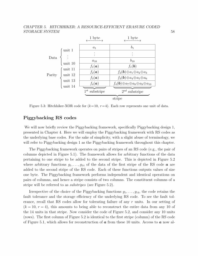
CHAPTER 5. HITCHHIKER: A RESOURCE-EFFICIENT ERASURE CODEDSTORAGE SYSTEM 58
unit 1
Data...
unit 10
unit 11
Parity unit 12
unit 13
unit 14
1 byte �����! 1 byte �����!
a1
b1
......
a10
b10
f1
(a) f1
(b)
f2
(a) f2
(b)�a1
�a2
�a3
f3
(a) f3
(b)�a4
�a5
�a6
f4
(a) f4
(b)�a7
�a8
�a9
�a10
| {z }1st substripe
| {z }2nd substripe
| {z }stripe
Figure 5.3: Hitchhiker-XOR code for (k=10, r=4). Each row represents one unit of data.
Piggybacking RS codes
We will now briefly review the Piggybacking framework, specifically Piggybacking design 1,presented in Chapter 4. Here we will employ the Piggybacking framework with RS codes asthe underlying base codes. For the sake of simplicity, with a slight abuse of terminology, wewill refer to Piggybacking design 1 as the Piggybacking framework throughout this chapter.
The Piggybacking framework operates on pairs of stripes of an RS code (e.g., the pair ofcolumns depicted in Figure 5.1). The framework allows for arbitrary functions of the datapertaining to one stripe to be added to the second stripe. This is depicted in Figure 5.2where arbitrary functions g
1
, . . . , g14
of the data of the first stripe of the RS code a areadded to the second stripe of the RS code. Each of these functions outputs values of sizeone byte. The Piggybacking framework performs independent and identical operations onpairs of columns, and hence a stripe consists of two columns. The constituent columns of astripe will be referred to as substripes (see Figure 5.2).
Irrespective of the choice of the Piggybacking functions g1
, . . . , g14
, the code retains thefault tolerance and the storage e�ciency of the underlying RS code. To see the fault tol-erance, recall that RS codes allow for tolerating failure of any r units. In our setting of(k = 10, r = 4), this amounts to being able to reconstruct the entire data from any 10 ofthe 14 units in that stripe. Now consider the code of Figure 5.2, and consider any 10 units(rows). The first column of Figure 5.2 is identical to the first stripe (column) of the RS codeof Figure 5.1, which allows for reconstruction of a from these 10 units. Access to a now al-
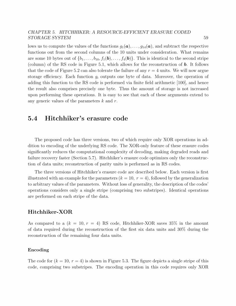
CHAPTER 5. HITCHHIKER: A RESOURCE-EFFICIENT ERASURE CODEDSTORAGE SYSTEM 59
lows us to compute the values of the functions g1
(a), . . . , g14
(a), and subtract the respectivefunctions out from the second columns of the 10 units under consideration. What remainsare some 10 bytes out of {b
1
, . . . , b10
, f1
(b), . . . , f4
(b)}. This is identical to the second stripe(column) of the RS code in Figure 5.1, which allows for the reconstruction of b. It followsthat the code of Figure 5.2 can also tolerate the failure of any r = 4 units. We will now arguestorage e�ciency. Each function g
i
outputs one byte of data. Moreover, the operation ofadding this function to the RS code is performed via finite field arithmetic [100], and hencethe result also comprises precisely one byte. Thus the amount of storage is not increasedupon performing these operations. It is easy to see that each of these arguments extend toany generic values of the parameters k and r.
5.4 Hitchhiker’s erasure code
The proposed code has three versions, two of which require only XOR operations in ad-dition to encoding of the underlying RS code. The XOR-only feature of these erasure codessignificantly reduces the computational complexity of decoding, making degraded reads andfailure recovery faster (Section 5.7). Hitchhiker’s erasure code optimizes only the reconstruc-tion of data units; reconstruction of parity units is performed as in RS codes.
The three versions of Hitchhiker’s erasure code are described below. Each version is firstillustrated with an example for the parameters (k = 10, r = 4), followed by the generalizationto arbitrary values of the parameters. Without loss of generality, the description of the codes’operations considers only a single stripe (comprising two substripes). Identical operationsare performed on each stripe of the data.
Hitchhiker-XOR
As compared to a (k = 10, r = 4) RS code, Hitchhiker-XOR saves 35% in the amountof data required during the reconstruction of the first six data units and 30% during thereconstruction of the remaining four data units.
Encoding
The code for (k = 10, r = 4) is shown in Figure 5.3. The figure depicts a single stripe of thiscode, comprising two substripes. The encoding operation in this code requires only XOR

CHAPTER 5. HITCHHIKER: A RESOURCE-EFFICIENT ERASURE CODEDSTORAGE SYSTEM 60
unit 1...
unit 10
unit 11
unit 12
unit 13
unit 14
a1
b1
......
a10
b10
f1
(a) f1
(b)L
10
i=4
ai
�L
10
i=1
bi
L10
i=1
bi
�L
3
i=1
ai
f3
(a) f3
(b)�L
6
i=4
ai
f4
(a) f4
(b)�L
9
i=7
ai
Figure 5.4: Hitchhiker-XOR+ for (k=10,r=4). Parity 2 of the underlying RS code is all-XOR.
unit 1...
unit 10
unit 11
unit 12
unit 13
unit 14
a1
b1
......
a10
b10
f1
(a) f1
(b)
f2
(0,0,0,a4
,...,a10
)�f2
(b) f2
(b)�f2
(a1
,a2
,a3
,0,...,0)
f3
(a) f3
(b)�f2
(0,0,0,a4
,a5
,a6
,0,...,0)
f4
(a) f4
(b)�f2
(0,...,0,a7
,a8
,a9
,0)
Figure 5.5: Hitchhiker-nonXOR code for (k=10,r=4). This can be built on any RS code. Eachrow is one unit of data.
operations in addition to the underlying RS encoding.
Reconstruction
First consider reconstructing the first unit. This requires reconstruction of {a1
, b1
} from theremaining units. Hitchhiker-XOR accomplishes this using only 13 bytes from the other units:the bytes belonging to both the substripes of units {2, 3} and the bytes belonging to only thesecond substripe of units {4, . . . , 12}. These 13 bytes are {a
2
, a3
, b2
, b3
. . . , b10
, f1
(b), f2
(b)�a1
� a2
� a3
}. The decoding procedure comprises three steps. Step 1: observe that the 10bytes {b
2
, . . . , b10
, f1
(b)} are identical to the corresponding 10 bytes in the RS encoding ofb (Figure 5.1). RS decoding of these 10 bytes gives b (and this includes one of the desiredbytes b
1
). Step 2: XOR f2
(b) with the second byte (f2
(b) � a1
� a2
� a3
) of the 12th unit.This gives (a
1
� a2
� a3
). Step 3: XORing this with a2
and a3
gives a1
. Thus both a1
andb1
are reconstructed by using only 13 bytes, as opposed to 20 bytes in RS codes, resultingin a saving of 35%.
CHAPTER 5. HITCHHIKER: A RESOURCE-EFFICIENT ERASURE CODEDSTORAGE SYSTEM 61
Let us now consider the reconstruction of any unit i 2 {1, . . . , 10}, which requires re-construction of {a
i
, bi
}. We shall first describe what data (from the other units) is re-quired for the reconstruction, following which we describe the decoding operation. Anydata unit i 2 {1, 2, 3} is reconstructed using the following 13 bytes: the bytes of both thesubstripes of units {1, 2, 3}\{i}, and the bytes belonging to only the second substripe fromunits {4, . . . , 12}.3 Any data unit i 2 {4, 5, 6} is also reconstructed using only 13 bytes:the bytes belonging to both the substripes of units {4, 5, 6}\{i}, and the bytes belonging toonly the second substripe of units {1, 2, 3, 7, . . . , 11, 13}. Any data unit i 2 {7, 8, 9, 10} isreconstructed using 14 bytes: both substripes of units {7, 8, 9, 10}\{i}, and only the secondsubstripe of units {1, . . . , 6, 11, 14}.
Three-step decoding procedure:Step 1: The set of 10 bytes {b
1
, . . . , b10
, f1
(b)}\{bi
} belonging to the second substripe ofthe units {1, . . . , 11}\{i} is identical to the 10 corresponding encoded bytes in the RS code.Perform RS decoding of these 10 bytes to get b (which includes one of the desired bytes b
i
).Step 2: In the other bytes accessed, subtract out all components that involve b.Step 3: XOR the resulting bytes to get a
i
.
Observe that during the reconstruction of any data unit, the remaining data units do notperform any computation. This property is termed ‘repair-by-transfer’ [149], and it carriesover to all three versions of Hitchhiker’s erasure code.
Hitchhiker-XOR+
Hitchhiker-XOR+ further reduces the amount of data required for reconstruction as com-pared to Hitchhiker-XOR, and employs only additional XOR operations. It however requiresthe underlying RS code to possess a certain property. This property, which we term the all-XOR-parity property, requires at least one parity function of the RS code to be an XOR ofall the data units. That is, a (k, r) RS code satisfying all-XOR-parity will have one of ther parity bytes as an XOR of all the k data bytes. For (k = 10, r = 4), Hitchhiker-XOR+requires 35% lesser data for reconstruction of any of the data units as compared to RS codes.
Encoding
The (k = 10, r = 4) Hitchhiker-XOR+ code is shown in Figure 5.4. The Hitchhiker-XOR+code is obtained by performing one additional XOR operation on top of Hitchhiker-XOR:in the second parity of Hitchhiker-XOR, the byte of the second substripe is XORed onto
3For any set A and any element i 2 A, the notation A\{i} denotes all elements of A except i.

CHAPTER 5. HITCHHIKER: A RESOURCE-EFFICIENT ERASURE CODEDSTORAGE SYSTEM 62
the byte of the first substripe to give Hitchhiker-XOR+. The underlying RS code in thisexample satisfies the all-XOR-parity property with its second parity function f
2
being anXOR of all the inputs.
We now argue that this additional XOR operation does not violate the fault tolerancelevel and storage e�ciency. To see fault tolerance, observe that the data of the second parityunit of Hitchhiker-XOR+ can always be converted back to that under Hitchhiker-XOR byXORing its second substripe with its first substripe. It follows that the data in any unitunder Hitchhiker-XOR+ is equivalent to the data in the corresponding unit in Hitchhiker-XOR. The fault tolerance properties of Hitchhiker-XOR thus carry over to Hitchhiker-XOR+.Storage e�ciency is retained because the additional XOR operation does not increase thespace requirement.
Decoding
The recovery of any unit i requires 13 bytes from the other units. The choice of the bytesto be accessed depends on the value of i, and is described below. The bytes required forthe reconstruction of any data unit i 2 {1, . . . , 6} are identical to that in Hitchhiker-XOR.Any data unit i 2 {7, 8, 9} is reconstructed using the following 13 bytes: the bytes ofboth substripes of units {7, 8, 9}\{i}, and the bytes of only the second substripes of units{1, . . . , 6, 10, 11, 14}. The tenth unit is also reconstructed using only 13 bytes: the bytesof only the second substripes of units {1, . . . , 9, 11, 13, 14}, and the byte of only the firstsubstripe of unit 12. The decoding procedure that operates on these 13 bytes is identical tothe three-step decoding procedure described above.
Hitchhiker-nonXOR
We saw that Hitchhiker-XOR+ results in more savings as compared to Hitchhiker-XOR, butrequires the underlying RS code to have the all-XOR-parity property. Hitchhiker-nonXORpresented here guarantees the same savings as Hitchhiker-XOR+ even when the underlyingRS code does not possess the all-XOR-parity property, but at the cost of additional finite-field arithmetic. Hitchhiker-nonXOR can thus be built on top of any RS code. It o↵ers asaving of 35% during the reconstruction of any data unit.
Encoding
The code for (k = 10, r = 4) is shown in Figure 5.5. As in Hitchhiker-XOR, in the secondparity, the first byte is XORed with the second byte. The final value of the second parity

CHAPTER 5. HITCHHIKER: A RESOURCE-EFFICIENT ERASURE CODEDSTORAGE SYSTEM 63
as shown in Figure 5.5 is a consequence of the fact that f2
(a) � f2
(a1
, a2
, a3
, 0, . . . , 0) =f2
(0, 0, 0, a4
, . . . , a10
) due to the linearity of RS encoding (this is discussed in greater detailin Section 5.6).
Decoding
Recovery of any unit requires only 13 bytes from other units. This set of 13 bytes is thesame as in Hitchhiker-XOR+. The decoding operation is a three-step procedure. The firsttwo steps are identical to the first two steps of the decoding procedure of Hitchhiker-XORdescribed above. The third step is slightly di↵erent, and requires an RS decoding operation(for units 1 to 9), as described below.
During reconstruction of any unit i 2 {1, 2, 3}, the output of the second step is the set ofthree bytes {a
1
, a2
, a3
, f1
(a1
, a2
, a3
, 0, . . . , 0)}\{ai
}. This is equivalent to having some 10 ofthe 11 bytes of the set {a
1
, a2
, a3
, 0, . . . , 0, f1
(a1
, a2
, a3
, 0, . . . , 0)}. Now, this set of 11 bytes isequal to the set of first 11 bytes of the RS encoding of {a
1
, a2
, a3
, 0, . . . , 0}. An RS decodingoperation thus gives {a
1
, a2
, a3
} which contains the desired byte ai
. Recovery of any otherunit i 2 {4, . . . , 9} follows along similar lines.
During the reconstruction of unit 10, the output of the second step is f1
(0, . . . , 0, a10
).Hence the third step involves only a single (finite-field) multiplication operation.
Generalization to any (k, r)
The encoding and decoding procedures for the general case follow along similar lines as theexamples discussed above, and are formally described below. In each of the three versions,the amount of data required for reconstruction is reduced by 25% to 45% as compared toRS codes, depending on the values of the parameters k and r. For instance, (k = 6, r =3) provides a saving of 25% with Hitchhiker-XOR and 34% with Hitchhiker-XOR+ andHitchhiker-nonXOR; (k = 20, r = 5) provides a savings of 37.5% with Hitchhiker-XOR and40% with Hitchhiker-XOR+ and Hitchhiker-nonXOR.
Hitchhiker-XOR: The encoding procedure of Hitchhiker-XOR first divides the k dataunits into (r� 1) disjoint sets of roughly equal sizes. For instance, in the (k=10, r=4) codeof Figure 5.3, the three sets are units {1, 2, 3}, units {4, 5, 6} and units {7, 8, 9, 10}. For eachset j 2 {1, . . . , r � 1}, the bytes of the first substripe of all units in set j are XORed, andthe resultant is XORed with the second substripe of the (j + 1)th parity unit.
Reconstruction of a data unit belonging to any set j requires the bytes of both thesubstripes of the other data units in set j, only the second byte of all other data units,

CHAPTER 5. HITCHHIKER: A RESOURCE-EFFICIENT ERASURE CODEDSTORAGE SYSTEM 64
and the second bytes of the first and (j + 1)th parity units. The decoding procedure forreconstruction of any data unit i is executed in three steps:Step 1 : The k bytes {b
1
, . . . , bk
, f1
(b)}\{bi
} belonging to the second substripe of the units{1, . . . , k + 1}\{i} are identical to the k corresponding encoded bytes in the underlying RScode. Perform RS decoding of these k bytes to get b (which includes one of the desired bytesbi
).Step 2 : In the other bytes accessed, subtract out all components that involve b.Step 3 : XOR the resulting bytes to get a
i
.
If the size of a set is s, reconstruction of any data unit in this set requires (k + s) bytes(as compared to 2k under RS codes).
Hitchhiker-XOR+: Assume without loss of generality that, in the underlying RScode, the all-XOR property is satisfied by the second parity. The encoding procedure firstselects a number ` 2 {0, . . . , k} and partitions the first (k� `) data units into (r� 1) sets ofroughly equal sizes. On these (k� `) data units and r parity units, it performs an encodingidentical to that in Hitchhiker-XOR. Next, in the second parity unit, the byte of the secondsubstripe is XORed onto the byte of the first substripe.
Reconstruction of any of the first (k� `) data units is performed in a manner identical tothat in Hitchhiker-XOR. Reconstruction of any of the last ` data units requires the byte of thefirst substripe of the second parity and the bytes of the second substripes of all other units.The decoding procedure remains identical to the three-step procedure of Hitchhiker-XORstated above.
For any of the first (k� `) data units, if the size of its set is s then reconstruction of thatdata unit requires (k+ s) bytes (as compared to 2k under RS). The reconstruction of any ofthe last ` units requires (k+ r+ `�2) bytes (as compared to 2k under RS). The parameter `can be chosen to minimize the average or maximum data required for reconstruction as perthe system requirements.
Hitchhiker-nonXOR: The encoding procedure is identical to that ofHitchhiker-XOR+, except that instead of XORing the bytes of the first substripe of thedata units in each set, these bytes are encoded using the underlying RS encoding functionconsidering all other data units that do not belong to the set as zeros.
The collection of data bytes required for the reconstruction of any data unit is identicalto that under Hitchhiker-XOR+. The decoding operation for reconstruction is a three-stepprocedure. The first two steps are identical to the first two steps of the decoding procedure ofHitchhiker-XOR described above. The third step requires an RS decoding operation (recallfrom the (k = 10, r = 4) case described above). In particular, the output of the second stepwhen reconstructing a data unit i will be equal to k bytes that would have been obtained

CHAPTER 5. HITCHHIKER: A RESOURCE-EFFICIENT ERASURE CODEDSTORAGE SYSTEM 65
from the RS encoding of the data bytes in the units belonging to that set with all otherdata bytes set to zero. An RS decoding operation performed on these bytes now gives a
i
,thus recovering the ith data unit (recall that b
i
is reconstructed in Step 1 itself.) The dataaccess patterns during reconstruction and the amount of savings under Hitchhiker-nonXORare identical to that under Hitchhiker-XOR+.
5.5 “Hop-and-Couple” for disk e�ciency
The description of the codes in Section 5.3 and Section 5.4 considers only two bytes per dataunit. We now move on to consider the more realistic scenario where each of the k data unitsto be encoded is larger (than two bytes). In the encoding process, these k data units arefirst partitioned into stripes, and identical encoding operations are performed on each of thestripes. The RS code considers one byte each from the k data units as a stripe. On theother hand, Hitchhiker’s erasure code has two substripes within a stripe (Section 5.4), andhence it couples pairs of bytes within each of the k data units to form the substripes of astripe. We will shortly see that the choice of the bytes to be coupled plays a crucial role indetermining the e�ciency of disk reads during reconstruction.
A natural strategy for forming the stripes for Hitchhiker’s erasure code is to coupleadjacent bytes within each unit, with the first stripe comprising the first two bytes of eachof the units, the second stripe comprising the next two bytes, and so on. Figure 5.6a depictssuch a method of coupling for (k = 10, r = 4). In the figure, the bytes accessed duringthe reconstruction of the first data unit are shaded. This method of coupling, however,results in highly discontiguous reads during reconstruction: alternate bytes are read fromunits 4 to 12 as shown in the figure. This high degree of discontinuity is detrimental to diskread performance, and forfeits the potential savings in disk IO during data reconstruction.The issue of discontiguous reads due to coupling of adjacent bytes is not limited to thereconstruction of the first data unit - it arises during reconstruction of any of the data units.
In order to ensure that the savings o↵ered by Hitchhiker’s erasure codes in the amount ofdata read during reconstruction are e↵ectively translated to gains in disk read e�ciency, wepropose a coupling technique for forming stripes that we call hop-and-couple. This techniqueaims to minimize the degree of discontinuity in disk reads during the reconstruction of dataunits. The hop-and-couple technique couples a byte with another byte within the sameunit that is a certain distance ahead (with respect to the natural ordering of bytes within aunit), i.e., it couples bytes after “hopping” a certain distance. We term this distance as thehop-length. This technique is illustrated in Figure 5.6b, where the hop-length is chosen to

CHAPTER 5. HITCHHIKER: A RESOURCE-EFFICIENT ERASURE CODEDSTORAGE SYSTEM 66
…
. . .
. . .
. . .
. . .
. . .
. . .
. . .
. . .
. . .
coupled bytes (encoded together)
unit 1 unit 2
unit 10
unit 14
unit 3
…
unit 4
unit 12 unit 13
…
. . .
. . .
. . .
. . .
. . .
. . .
. . .
. . .
. . . . . .
hop length
unit 1 unit 2
unit 10 unit 11
unit 14
…
data units
parity units
unit 3
…
unit 4
unit 12 unit 13
. . .
. . .
. . .
. . .
. . .
. . .
. . .
. . .
1 byte
coupled bytes (encoded together)
(a) coupling adjacent bytes to form stripes (b) hop-and-couple
. . .
. . . . . .
unit 11
data units
parity units
Figure 5.6: Two ways of coupling bytes to form stripes for Hitchhiker’s erasure code. The shadedbytes are read and downloaded for the reconstruction of the first unit. While both methods requirethe same amount of data to be read, the reading is discontiguous in (a), while (b) ensures that thedata to be read is contiguous.
be half the size of a unit.
The hop-length may be chosen to be any number that divides B
2
, where B denotes thesize of each unit. This condition ensures that all the bytes in the unit are indeed coupled.Coupling adjacent bytes (e.g., Figure 5.6a) is a degenerate case where the hop-length equals1. The hop-length significantly a↵ects the contiguity of the data read during reconstructionof the data units, in that the data is read as contiguous chunks of size equal to the hop-length. For Hitchhiker’s erasure codes, a hop-length of B
2
minimizes the total number ofdiscontiguous reads required during the reconstruction of data units. While higher values ofhop-length reduces the number of discontiguous reads, it results in bytes further apart beingcoupled to form stripes. This is a trade-o↵ to be considered when choosing the value of thehop-length, and is discussed further in Section 5.8.
We note that the reconstruction operation under RS codes reads the entire data from k ofthe units, and hence trivially, the reads are contiguous. On the other hand, any erasure codethat attempts to make reconstruction more e�cient by downloading partial data from theunits (e.g.,[89, 127, 149, 150, 115, 169, 72]) will encounter the issue of discontiguous reads, asin Hitchhiker’s erasure code. Any such erasure code would have multiple (say, ↵) substripesin every stripe and would read a subset of these substripes from each of the units duringreconstruction. The hop-and-couple technique can be applied to any such erasure code totranslate the network savings to disk savings as well. The hop-length can be chosen to beany number that divides B
↵
. As in the case of Hitchhiker’s erasure codes (where ↵ = 2), thiscondition ensures that all the bytes are indeed coupled. If the bytes to be coupled are chosen
CHAPTER 5. HITCHHIKER: A RESOURCE-EFFICIENT ERASURE CODEDSTORAGE SYSTEM 67
with hop-length equal to B/↵, then the hop-and-couple technique would ensure that all thebytes of a substripe are contiguous within any unit. Reading a substripe from a unit wouldthen result in a contiguous disk read, thereby minimizing the total degree of discontiguityin disk reads during reconstruction.
5.6 Implementation
We have implemented Hitchhiker in the Hadoop Distributed File System (HDFS). HDFS-RAID [67] is a module in HDFS that deals with erasure codes and is based on [51]. Thismodule forms the basis for the erasure-coded storage system employed in the data-warehousecluster at Facebook, and is open sourced under Apache. HDFS-RAID deployed at Facebookis based on RS codes, and we will refer to this system as RS-based HDFS-RAID. Hitchhikerbuilds on top of RS codes, and the present implementation uses the RS encoder and decodermodules of RS-based HDFS-RAID as its building blocks.
Brief description of HDFS-RAID
HDFS stores each file by dividing it into blocks of a certain size. By default, the size of eachblock is 256 MB, and this is also the value that is typically used in practice. In HDFS, threereplicas of each block are stored in the system by default. HDFS-RAID o↵ers RS codes asan alternative to replication for maintaining redundancy.
The relevant modules of HDFS-RAID and the execution flows for relevant operations aredepicted in Figure 5.7. The RAID-Node manages all operations related to the use of erasurecodes in HDFS. It has a list of files that are to be converted from the replicated state to theerasure-coded state, and periodically performs encoding of these files via MapReduce jobs.Sets of k blocks from these files are encoded to generate r parity blocks each.4 Once the r
parity blocks of a set are successfully written into the file system, the replicas of the k datablocks of that set are deleted. The MapReduce job calls the Encoder of the erasure code toperform encoding. The Encoder uses the Parallel-Reader to read the data from the k blocksthat are to be encoded. The Parallel-Reader opens k parallel streams, issues HDFS readrequests for these blocks, and puts the data read from each stream into di↵erent bu↵ers.Typically, the bu↵ers are 1 MB each. When one bu↵er-sized amount of data is read fromeach of the k blocks, the Encoder performs the computations pertaining to the encodingoperation. This process is repeated until the entire data from the k blocks are encoded.
4In the context of HDFS, the term block corresponds to a unit and we will use these terms interchangeably.
CHAPTER 5. HITCHHIKER: A RESOURCE-EFFICIENT ERASURE CODEDSTORAGE SYSTEM 68
RAID%File%System%
Erasure%code%Encoder%
Erasure%code%Decoder%
Parallel%Reader%
HDFS-RAID
HDFS
RAID%Node%
Degraded read Recovery Encoding
Legend
Figure 5.7: Relevant modules in HDFS-RAID. The execution flow for encoding, degraded readsand reconstruction operations are shown. Hitchhiker is implemented in the shaded modules.
The RAID-Node also handles recovery operations, i.e., reconstructing missing blocks inorder to maintain the reliability of the system. The RAID-Node has a list of blocks that aremissing and need to be recovered. It periodically goes through this list and reconstructs theblocks by executing a MapReduce job. The MapReduce job calls the Decoder of the erasurecode to perform the reconstruction operation. The Decoder uses the Parallel-Reader to readthe data required for reconstruction. For an RS code, data from k blocks belonging to thesame set as that of the block under reconstruction is read in parallel. As in the encodingprocess, data from the k blocks are read into bu↵ers, and the computations are performedonce one bu↵er size amount of data is read from each of the k blocks. This is repeated untilthe entire block is reconstructed.
HDFS directs any request for a degraded read (i.e., a read request for a block that isunavailable) to the RAID File System. The requested block is reconstructed on the fly bythe RAID-Node via a MapReduce job. The execution of this reconstruction operation isidentical to that in the reconstruction process discussed above.
Hitchhiker in HDFS
We implemented Hitchhiker in HDFS making use of the new erasure code constructedusing the Piggybacking framework (Section 5.4) and the hop-and-couple technique (Sec-tion 5.5). We implemented all three versions of the proposed storage code: Hitchhiker-XOR,Hitchhiker-XOR+, and Hitchhiker-nonXOR. This required implementing new Encoder, De-

CHAPTER 5. HITCHHIKER: A RESOURCE-EFFICIENT ERASURE CODEDSTORAGE SYSTEM 69
coder and Parallel-Reader modules (shaded in Figure 5.7), entailing 7k lines of code. Theimplementation details described below pertain to parameters (k = 10, r = 4) which arethe default parameters in HDFS. We emphasize that, however, Hitchhiker is generic andsupports all values of the parameters k and r.
Hitchhiker-XOR and Hitchhiker-XOR+
The implementation of these two versions of Hitchhiker is exactly as described in Section 5.4and Section 5.4 respectively.
Hitchhiker-nonXOR
Hitchhiker-nonXOR requires finite field arithmetic operations to be performed in additionto the operations performed for the underlying RS code. We now describe how our imple-mentation executes these operations.
Encoder: As seen in Figure 5.5, in addition to the underlying RS code, the Encoderneeds to compute the functions f
2
(a1
,a2
,a3
,0...,0), f2
(0,...,0,a4
,a5
,a6
,0...,0), andf2
(0,...,0,a7
,a8
,a9
,0), where f2
is the second parity function of the RS code. One way toperform these computations is to simply employ the existing RS encoder. This approach,however, involves computations that are superfluous to our purpose: The RS encoder usesan algorithm based on polynomial computations [100] that inherently computes all thefour parities f
1
(x), f2
(x), f3
(x), and f4
(x) for any given input x. On the other hand, werequire only one of the four parity functions for each of the three distinct inputs(a
1
,a2
,a3
,0...,0), (0,...,0,a4
,a5
,a6
,0...,0) and (0,...,0,a7
,a8
,a9
,0). Furthermore, these inputs aresparse, i.e., most of the input bytes are zeros.
Our Encoder implementation takes a di↵erent approach, exploiting the fact that RS codeshave the property of linearity, i.e., each of the parity bytes of an RS code can be writtenas a linear combination of the data bytes. Any parity function f
`
can thus be specified asf`
(x) =L
10
j=1
c`,j
xj
for some constants c`,1
, . . . , c`,10
. We first inferred the values of theseconstants for each of the parity functions (from the existing “black-box” RS encoder) in thefollowing manner. We first fed the input [1 0 · · · 0] to the encoder. This gives the constantsc1,1
, . . . , c4,1
as the values of the four parities respectively in the output from the encoder.The values of the other constants were obtained in a similar manner by feeding di↵erent unitvectors as inputs to the encoder. Note that obtaining the values of these constants from the“black-box” RS encoder is a one-time task. With these constants, the encoder computesthe desired functions simply as linear combinations of the given data units (for example, wecompute f
2
(a1
, a2
, a3
, 0 . . . , 0) simply as c2,1
a1
� c2,2
a2
� c2,3
a3
).

CHAPTER 5. HITCHHIKER: A RESOURCE-EFFICIENT ERASURE CODEDSTORAGE SYSTEM 70
Decoder: As seen in Section 5.4, during reconstruction of any of the first nine units,the first byte is reconstructed by performing an RS decoding of the data obtained in theintermediate step. One straightforward way to implement this is to use the existing RSdecoder for this operation. However, we take a di↵erent route towards a computationallycheaper option. We make use of two facts: (a) Observe from the description of the recon-struction process (Section 5.4) that for this RS decoding operation the data is known to be‘sparse’, i.e., contains many zeros, and (b) the RS code has the linearity property, and fur-thermore, any linear combination of zero-valued data is zero. Motivated by this observation,our Decoder simply inverts this sparse linear combination to reconstruct the first substripein a more e�cient manner.
Hop-and-couple
Hitchhiker uses the proposed hop-and-couple technique to couple bytes during encoding. Weuse a hop-length of half a block since the granularity of data read requests and recovery inHDFS is typically an entire block. As discussed in Section 5.5, this choice of the hop-lengthminimizes the number of discontiguous reads. However, the implementation can be easilyextended to other hop-lengths as well.
When the block size is larger than the bu↵er size, coupling bytes that are half a blockapart requires reading data from two di↵erent locations within a block. In Hitchhiker, thisis handled by the Parallel-Reader.
Data read patterns during reconstruction
During reconstruction in Hitchhiker, the choice of the blocks from which data is read, theseek locations, and the amount of data read are determined by the identity of the blockbeing reconstructed. Since Hitchhiker uses the hop-and-couple technique for coupling bytesto form stripes during encoding, the reads to be performed during reconstruction are alwayscontiguous within any block (Section 5.5).
For reconstruction of any of the first nine data blocks in Hitchhiker-XOR+ or Hitchhiker-nonXOR or for reconstruction of any of the first six data blocks in Hitchhiker-XOR, Hitch-hiker reads and downloads two full blocks (i.e., both substripes) and nine half blocks (onlythe second substripes). For example, the read patterns for decoding blocks 1 and 4 areas shown in Figure 5.8a and 5.8b respectively. For reconstruction of any of the last fourdata blocks in Hitchhiker-XOR, Hitchhiker reads and downloads three full blocks (both sub-stripes) and nine half blocks (only the second substripes). For recovery of the tenth data

CHAPTER 5. HITCHHIKER: A RESOURCE-EFFICIENT ERASURE CODEDSTORAGE SYSTEM 71
block 10 block 11
block 14 256 MB
block 13 block 12
block 9 block 8 block 7 block 6 block 5 block 4
block 2 block 1
block 3
256 MB 256 MB (a) block 1 (b) block 4 (c) block 10
data
parity
Figure 5.8: Data read patterns during reconstruction of blocks 1, 4 and 10 in Hitchhiker-XOR+:the shaded bytes are read and downloaded.
block in Hitchhiker-XOR+ or Hitchhiker-nonXOR, Hitchhiker reads half a block each fromthe remaining thirteen blocks. This read pattern is shown in Figure 5.8c.
5.7 Evaluation
Evaluation setup and metrics
We evaluate Hitchhiker using two HDFS clusters at Facebook: (i) the data-warehouse clusterin production comprising multiple thousands of machines, with ongoing real-time tra�c andworkloads, and (ii) a smaller test cluster comprising around 60 machines. In both theclusters, machines are connected to a rack switch through 1Gb/s Ethernet links. The higherlevels of the network tree architecture have 8Gb/s Ethernet connections.
We compare Hitchhiker and RS-based HDFS-RAID in terms of the time taken for compu-tations during encoding and reconstruction, the time taken to read the requisite data duringreconstruction, and the amount of data that is read and transferred during reconstruction.5
Note that in particular, the computation and the data read times during reconstruction arevital since they determine the performance of the system during degraded reads and recovery.
5Both systems read the same data during encoding, and are hence trivially identical on this metric.

CHAPTER 5. HITCHHIKER: A RESOURCE-EFFICIENT ERASURE CODEDSTORAGE SYSTEM 72
Evaluation methodology
We first deployed HDFS-RAID with both Hitchhiker and the RS-based system on a 60-machine test cluster at Facebook in order to verify Hitchhiker’s end-to-end functionality.We created multiple files with a block size of 256MB, and encoded them separately usingHitchhiker and RS-based HDFS-RAID. The block placement policy of HDFS-RAID ensuresthat the 14 blocks of an encoded stripe are all stored on di↵erent machines. We thenforced some of these machines to become unavailable by stopping HDFS related scriptsrunning on them, and collected the logs pertaining to the MapReduce jobs that performedthe reconstruction operations. We verified that all reconstruction operations were successful.We also confirmed that the amount of data read and downloaded in Hitchhiker was 35% lowerthan in RS-based HDFS-RAID, as guaranteed by the proposed codes. We do not performtiming measurements on the test cluster since the network tra�c and the workload on thesemachines do not reflect the real (production) scenario. Instead, we evaluated these metricsdirectly on the production cluster itself as discussed below.
The encoding and reconstruction operations in HDFS-RAID, including those for degradedreads and recovery, are executed as MapReduce jobs. The data-warehouse cluster does notmake any distinction between the MapReduce jobs fired by the RAID-Node and those firedby a user. This allows us to perform evaluations of the timing metrics for encoding, recovery,and degraded read operations by running them as MapReduce jobs on the production cluster.Thus evaluation of all the timing metrics is performed in the presence of real-time productiontra�c and workloads.
For all the evaluations, we consider the encoding parameters (k = 10, r = 4), a blocksize of 256 MB (unless mentioned otherwise), and a bu↵er size of 1 MB. These are thedefault parameters of HDFS-RAID. Moreover, these are the parameters employed in thedata-warehouse cluster in production at Facebook to store multiple tens of Petabytes.
In the evaluations, we show results of the timing metrics for one bu↵er size. This issu�cient since the same operations are performed repeatedly on one bu↵er size amount ofdata until an entire block is processed.
Computation time for degraded reads & recovery
Figure 5.9 shows the comparison of computation time during data reconstruction (from 200runs each). Note that (i) in both Hitchhiker-XOR+ and Hitchhiker-nonXOR, reconstructionof any of the first nine data blocks entails same amount of computation, (ii) reconstructionof any data block in Hitchhiker-XOR is almost identical to reconstruction of block 1 in

CHAPTER 5. HITCHHIKER: A RESOURCE-EFFICIENT ERASURE CODEDSTORAGE SYSTEM 73
Figure 5.9: A box plot comparing the computation time for reconstruction of 1MB (bu↵er size)from 200 runs each on Facebook’s data-warehouse cluster with real-time production tra�c andworkloads. (HH = Hitchhiker.)
Hitchhiker-XOR+. Hence, for brevity, no separate measurements are shown.
We can see that Hitchhiker’s erasure codes perform faster reconstruction than RS-basedHDFS-RAID for any data block. This is because (recall from Section 5.4) the reconstructionoperation in Hitchhiker requires performing the resource intensive RS decoding only forhalf the substripes as compared to RS-based HDFS-RAID. In Hitchhiker, the data in theother half of substripes is reconstructed by performing either a few XOR operations (underHitchhiker-XOR and Hitchhiker-XOR+) or a few finite-field operations (under Hitchhiker-nonXOR). One can also see that Hitchhiker-XOR+ has 25% lower computation time duringreconstruction as compared to Hitchhiker-nonXOR for the first nine data blocks; for block10, the time is almost identical in Hitchhiker-XOR+ and Hitchhiker-nonXOR (as expectedfrom theory (Section 5.4)).
Read time for degraded reads & recovery
Figure 5.12a and Figure 5.12b respectively compare the median and the 95th percentile ofthe read times during reconstruction for three di↵erent block sizes: 4MB, 64MB, and 256MBin Hitchhiker-XOR+. The read patterns for reconstruction of any of the first nine blocks areidentical (Section 5.4).
In the median read times for reconstruction of blocks 1-9 and block 10 respectively, in

CHAPTER 5. HITCHHIKER: A RESOURCE-EFFICIENT ERASURE CODEDSTORAGE SYSTEM 74
Figure 5.10: Median
Figure 5.11: 95th percentile
Figure 5.12: Total read time (in seconds) during reconstruction from 200 runs each on Facebook’sdata-warehouse cluster with real-time production tra�c and workloads. (HH = Hitchhiker.)
comparison to RS-based HDFS-RAID, we observed a reduction of 41.4% and 41% respec-tively for 4MB block size, 27.7% and 42.5% for 64MB block size, and 31.8% and 36.5% for256MB block size. For the 95th percentile of the read time we observed a reduction of 35.4%and 48.8% for 4MB, 30.5% and 29.9% for 64MB, and 30.2% and 31.2% for 256MB blocksizes.
The read pattern of Hitchhiker-nonXOR is identical to Hitchhiker-XOR+, while that ofHitchhiker-XOR is the same for the first six blocks and almost the same for the remainingfour blocks. Hence for brevity, we plot the statistics only for Hitchhiker-XOR+.
Although Hitchhiker reads data from more machines as compared to RS-based HDFS-RAID, we see that it gives a superior performance in terms of read latency during reconstruc-tion. The reason is that Hitchhiker reads only half a block size from most of the machinesit connects to (recall from Section 5.6) whereas RS-based HDFS-RAID reads entire blocks.

CHAPTER 5. HITCHHIKER: A RESOURCE-EFFICIENT ERASURE CODEDSTORAGE SYSTEM 75
Figure 5.13: A box plot comparing the computation time for encoding of 1MB (bu↵er size) from 200runs each on Facebook’s data-warehouse cluster with real-time production tra�c and workloads.(HH = Hitchhiker.)
Computation time for encoding
Figure 5.13 compares the computation time for the encoding operation. Hitchhiker en-tails higher computational overheads during encoding as compared to RS-based systems,and Hitchhiker-XOR+ and Hitchhiker-XOR are faster than the Hitchhiker-nonXOR. Thisis expected since Hitchhiker’s encoder performs computations in addition to those of RSencoding. Section 5.8 discusses the tradeo↵s between higher encoding time and savings inother metrics.
5.8 Discussion
In this section, we discuss the various tradeo↵s a↵orded by Hitchhiker.
a) Three versions of the code: During encoding and reconstruction, Hitchhiker-XOR re-quires performing only XOR operations in addition to the operations of the underlying RScode. Hitchhiker-XOR+ allows for more e�cient reconstruction in terms of network and diskresources in comparison to Hitchhiker-XOR, while still using only XOR operations in addi-tion to the RS code’s operations. Hitchhiker-XOR+, however, requires the underlying RScode to satisfy the all-XOR-parity property (Section 5.4). Hitchhiker-nonXOR provides the

CHAPTER 5. HITCHHIKER: A RESOURCE-EFFICIENT ERASURE CODEDSTORAGE SYSTEM 76
same e�ciency in reconstruction as Hitchhiker-XOR+ without imposing the all-XOR-parityrequirement on the RS code, but entails additional finite-field arithmetic during encodingand reconstruction.
b) Connecting to more machines during reconstruction: Reconstruction in RS-coded sys-tems requires connecting to exactly k machines, whereas Hitchhiker entails connecting tomore than k machines. In certain systems, depending on the setting at hand, this may leadto an increase in the read latency during reconstruction. However, in our experiments onthe production data-warehouse cluster at Facebook, we saw no such increase in read latency.On the contrary, we consistently observed a significant reduction in the latency due to thesignificantly lower amounts of data required to be read and downloaded in Hitchhiker (seeFigure 5.12).
c) Option of operating as an RS-based system: The storage overheads and fault toleranceof Hitchhiker are identical to RS-based systems. Moreover, a reconstruction operation inHitchhiker can alternatively be performed as in RS-based systems by downloading any k
entire blocks. Hitchhiker thus provides an option to operate as an RS-based system whennecessary, e.g., when increased connectivity during reconstruction is not desired. This featurealso ensures Hitchhiker’s compatibility with other alternative solutions proposed outside theerasure-coding component (e.g., [20, 102, 33]).
d) Choice of hop-length: As discussed in Section 5.5, a larger hop-length leads to morecontiguous reads, but requires coupling of bytes that are further apart. Recall that recon-structing any byte also necessitates reconstructing its coupled byte. In a scenario where onlya part of a block may need to be reconstructed, all the bytes that are coupled with the bytesof this part must also be reconstructed even if they are not required. A lower hop-lengthreduces the amount such unnecessary reconstructions.
5.9 Summary
In this chapter, we presented a systematically-designed, novel storage system, called Hitch-hiker, that “rides” on top of existing Reed-Solomon based erasure-coded systems utilizingthe Piggybacking framework presented in Chapter 4. Hitchhiker retains the key benefitsof RS-coded systems over replication-based counterparts, namely that of (i) optimal stor-age space needed for a targeted level of reliability, as well as (ii) complete flexibility in thedesign choice for the system parameters. We show how Hitchhiker can additionally reduceboth network tra�c and disk tra�c by 25% to 45% over that of RS-coded systems duringreconstruction of missing or otherwise unavailable data. Further, our implementation andevaluation of Hitchhiker on two HDFS clusters at Facebook also reveals savings of 36% in

CHAPTER 5. HITCHHIKER: A RESOURCE-EFFICIENT ERASURE CODEDSTORAGE SYSTEM 77
the computation time and 32% in the time taken to read data during reconstruction.
Hitchhiker is being incorporated into the next release of Apache Hadoop Distributed Filesystem (Apache HDFS).

78
Chapter 6
Optimizing I/O and CPU along withstorage and network bandwidth
In this chapter, we present erasure codes aimed at jointly optimizing the usage of storage,network, I/O and CPU resources. First, we design erasure codes that are simultaneouslyoptimal in terms of I/O, storage, and network usage. As a part of this design, we present atransformation that can be employed on existing classes of storage codes called minimum-storage-regenerating codes [41] in order to optimize their usage of I/O while retaining theiroptimal usage of storage and network. Through evaluations on Amazon EC2, we showthat the proposed design results in a significant reduction in IOPS (I/O operations persecond) during reconstructions: a 5⇥ reduction for typical parameters. Second, we showthat optimizing I/O and CPU go hand-in-hand in these resource-e�cient distributed storagecodes, by showing that our transformation that optimizes I/O also sparsifies the code therebyreducing the computational complexity.
6.1 Introduction
Recall from Chapter 2 that under RS codes, redundancy is introduced in the followingmanner: a file to be stored is divided into equal-sized units, which we will call blocks. Blocksare grouped into sets of k each, and for each such set of k blocks, r parity blocks arecomputed. The set of these (k + r) blocks consisting of both the data and the parity blocksconstitute a stripe. The data and parity blocks belonging to a stripe are placed on di↵erentnodes in the storage network, and these nodes are typically chosen from di↵erent racks.

CHAPTER 6. OPTIMIZING I/O AND CPU ALONG WITH STORAGE ANDNETWORK BANDWIDTH 79
1"he
lper
s!
decoding !node!
12"
8"
7"
6"
2"
1"
total"transfer"""""="96MB"
(a) RShelpers!
decoding!node!
1"
12"
8"
7"
6"
2"
1"
total"transfer""""="29.7MB"
(b) Minimum-storage-regenerating (MSR)code
Figure 6.1: Amount of data transfer involved in reconstruction of block 1 for an RS code withk = 6, r = 6 and an MSR code with k = 6, r = 6, d = 11, with blocks of size 16MB. The datablocks are shaded.
Also, recall that under traditional repair of RS codes, a missing block is replaced bydownloading all data from (any) k other blocks in the stripe and decoding the desired datafrom it. Let us look at an example. Consider an RS code with k = 6 and r = 6. While thiscode has a storage overhead of 2⇥, it o↵ers orders of magnitude higher reliability than 3⇥replication. Figure 6.1a depicts a stripe of this code, and also illustrates the reconstructionof block 1 using the data from blocks 2 to 7. Here, blocks 2 to 7 are the helpers. Inthis example, in order to reconstruct a 16 MB block, 6 ⇥ 16MB = 96 MB of data is readfrom disk at the helpers and transferred across the network to the node performing thedecoding computations. In general, the disk read and the network transfer overheads duringa reconstruction operation is k times that under replication. Consequently, under RS codes,reconstruction operations result in a large amount of disk I/O and network transfers, puttinga huge burden on these system resources.
Minimum-storage-regenerating (MSR) codes [41] are a recently proposed framework fordistributed storage codes that optimize storage and network-bandwidth usage during re-construction operations. Under an MSR code, an unavailable block is reconstructed bydownloading a small fraction of the data from any d (> k) blocks in the stripe, in a mannerthat the total amount of data transferred during reconstruction is lower than that in RS

CHAPTER 6. OPTIMIZING I/O AND CPU ALONG WITH STORAGE ANDNETWORK BANDWIDTH 80
codes. Let us consider an example with k = 6, r = 6 and d = 11. For these parameters,reconstruction of block 1 under an MSR code is illustrated in Figure 6.1b. In this example,the total network transfer is only 29.7 MB as opposed to 96 MB under RS. MSR codes areoptimal with respect to storage and network transfers: the storage capacity and reliabilityis identical to that under RS codes, while the network transfer is significantly lower thanthat under RS and in fact, is the minimum possible under any code. However, in general,MSR codes do not optimize the usage of I/Os. The I/O overhead during a reconstructionoperation in a system employing an MSR code is, in general, higher than that in a sys-tem employing RS code. This is illustrated in Figure 6.2a which depicts the amount dataread from disks for reconstruction of block 1 under a practical construction of MSR codescalled product-matrix-MSR (PM-MSR) codes. This entails reading 16 MB at each of the 11helpers, totaling 176 MB of data read. While under RS codes, the amount of data read isonly 96 MB.
I/Os are a valuable resource in storage systems. With the increasing speeds of newergeneration network interconnects and the increasing storage capacities of individual storagedevices, I/O is becoming the primary bottleneck in the performance of disk-based storagesystems. Moreover, many applications that the storage systems serve today are I/O bound,for example, applications that serve a large number of user requests [18]. Motivated by theincreasing importance of I/O, we investigate practical erasure codes for storage systems thatare also I/O optimal along with storage and network-bandwidth optimality.
Furthermore, one of the most frequent operations performed in distributed storage sys-tems is encoding of the new data entering the system. The CPU cost of encoding is anon-issue when using replication, but can be significant when using erasure codes. This canalso slow down the data ingestion process. Thus it is desirable for the storage code to possessa low-complexity, fast encoding operation. For any linear code, the encoding operation canbe represented as a matrix-vector multiplication between a matrix termed as the generatormatrix of the code and a vector consisting of data symbols to be encoded [100]. This encod-ing operation will be fast and less CPU intensive if the generator matrix is sparse, since thisreduces the number of computations to be performed.
In this chapter, we consider the problem of designing practical erasure codes that aresimultaneously optimal in terms of I/O, storage, and network bandwidth while also sup-porting fast encoding. To this end, we first identify two properties that aid in transformingMSR codes to be disk-read optimal during reconstruction while retaining their storage andnetwork optimality. We show that a class of powerful practical constructions for MSR codes,the product-matrix-MSR codes (PM-MSR) [127], indeed satisfy these desired properties. Wethen present an algorithm to transform any MSR code satisfying these properties into a codethat is optimal in terms of the amount of data read from disks. We apply our transformation

CHAPTER 6. OPTIMIZING I/O AND CPU ALONG WITH STORAGE ANDNETWORK BANDWIDTH 81
helpers!
16MB"read"
16MB"read"
16MB"read"
16MB"read"
16MB"read"
1"
12"
8"
7"
6"
2"total"data"read"
="176MB"
(a) PM-MSR
1"
helpers!
2.7MB"read"
2.7MB"read"
2.7MB"read"
2.7MB"read"
2.7MB"read"12"
8"
7"
6"
2"total"data"read"
="29.7MB"
(b) PM-RBT
Figure 6.2: Amount of data read from disks during reconstruction of block 1 for k = 6, r = 6,d = 11 with blocks of size 16 MB.
to PM-MSR codes and call the resulting I/O optimal codes as PM-RBT codes. Figure 6.2bdepicts the amount of data read for reconstruction of block 1 for the example parameters:PM-RBT entails reading only 2.7 MB at each of the 11 helpers, totaling 29.7 MB of dataread as opposed to 176 MB under PM-MSR. We note that the PM-MSR codes operate inthe regime r � k � 1, and consequently the PM-RBT codes also operate in this regime.
We implement PM-RBT codes in C/C++, and show through experiments on AmazonEC2 instances that our approach results in a 5⇥ reduction in I/Os consumed during recon-struction as compared to the original product-matrix codes, for a typical set of parameters.For general parameters, the number of I/Os consumed would reduce approximately by afactor of (d� k + 1). For typical values of d and k, this can result in substantial gains. Wethen show that if the relative frequencies of reconstruction of blocks are di↵erent, a moreholistic system-level design of helper assignments is needed to optimize I/Os across the entiresystem. Such situations are common: for instance, in a system that deals with degradedreads as well as node failures, the data blocks will be reconstructed more frequently than theparity blocks. We pose this problem as an optimization problem and present an algorithm toobtain the optimal solution to this problem. We evaluate our helper assignment algorithmthrough simulations using data from experiments on Amazon EC2 instances.
We then establish a general connection between optimizing I/O and reducing the encodingcomplexity, by showing that a specific transformation that we present for I/O optimizationin MSR codes leads to sparsity in the generator matrix of the code. Through evaluations on

CHAPTER 6. OPTIMIZING I/O AND CPU ALONG WITH STORAGE ANDNETWORK BANDWIDTH 82
Amazon EC2 using PM-MSR codes, we show that such a transformation leads to approxi-mately k⇥ reduction in the encoding complexity and thus a k⇥ speed up in the computationtime of the encoding process.
PM-RBT codes presented in this chapter provide higher savings in I/O and networkbandwidth as compared to Piggybacked-RS codes presented in Chapter 5. On the otherhand, Piggybacked-RS codes have the advantage of being applicable for all values of k andr, whereas PM-RBT codes are only applicable for d � (2k � 2) and thereby necessitate astorage overhead of atleast (2� 1
k
).
6.2 Related work
In [71], the authors build a file system based on the minimum-bandwidth-regenerating(MBR) code constructions of [149]. While this system minimizes network transfers andthe amount of data read during reconstruction, it mandates additional storage capacity toachieve the same. That is, the system is not optimal with respect to storage-reliability trade-o↵. The storage systems proposed in [73, 146, 49] employ a class of codes called local-repaircodes which optimize the number of blocks accessed during reconstruction. This, in turn,also reduces the amount of disk reads and network transfers. However, these systems alsonecessitate an increase in storage-space requirements in the form of at least 25% to 50% addi-tional parities. In [92], authors present a system which combines local-repair codes with thegraph-based MBR codes presented in [149]. This work also necessitates additional storagespace. The goal of the present chapter is to optimize I/Os consumed during reconstructionwithout losing the optimality with respect to storage-reliability tradeo↵.
In [72] and [11], the authors present storage systems based on random network-codingthat optimize resources consumed during reconstruction. Here the data that is reconstructedis not identical and is only “functionally equivalent” to the failed data. As a consequence,the system is not systematic, and needs to execute the decoding procedure for serving everyread request. The present chapter designs codes that are systematic, allowing read requestsduring the normal mode of operation to be served directly without executing the decodingprocedure.
In [150], the authors consider the theory behind reconstruction-by-transfer for MBRcodes, which as discussed earlier are not optimal with respect to storage-reliability tradeo↵.Some of the techniques employed in the current chapter are inspired by the techniques intro-duced in [150]. In [178] and [183], the authors present optimizations to reduce the amountof data read for reconstruction in array codes with two parities. The code constructions pro-

CHAPTER 6. OPTIMIZING I/O AND CPU ALONG WITH STORAGE ANDNETWORK BANDWIDTH 83
vided in [44, 119, 91, 160] optimize both I/O and network bandwidth during reconstruction.However, these codes are not MDS and thus necessitate additional storage overhead.
[89] presents a search-based approach to find reconstruction symbols that optimize I/Ofor arbitrary binary erasure codes, but this search problem is shown to be NP-hard. In[89], authors also present Rotated-RS codes which reduce the amount of data read duringrebuilding. However, the reduction achieved is significantly lower than that in PM-RBT.
Several works (e.g., [20, 102, 33]) have proposed system-level solutions to reduce networkand I/O consumption for reconstruction, such as caching the data read during reconstruction,batching multiple reconstruction operations, and delaying the reconstruction operations.While these solutions consider the erasure code as a black-box, our work optimizes thisblack-box and can be used in conjunction with these system-level solutions.
The computational complexity of the encoding operation can be reduced by decreasingthe field size over which the code is constructed as well as by making the generator matrixof the code sparse. There have been a number of recent works [47, 69, 137] on constructingMSR codes with small field size requirement. In this chapter, we look at sparsifying thegenerator matrix of MSR codes.
6.3 Background
Notation and terminology
We will refer the smallest granularity of the data in the system as a symbol. The actualsize of a symbol is dependent on the finite-field arithmetic that is employed. For simplicity,the reader may consider a symbol to be a single byte. A vector will be column vector bydefault. We will use boldface to denote column vectors, and use T to denote a matrix orvector transpose operation.
We will now introduce some more terminology in addition to that introduced in Sec-tion 6.1. This terminology is illustrated in Figure 6.3. Let n (= k + r) denote the totalnumber of blocks in a stripe. In order to encode the k data blocks in a stripe, each of thek data blocks are first divided into smaller units consisting of ↵ symbols each. A set of ↵symbols from each of the k blocks is encoded to obtain the corresponding set of ↵ symbolsin the parity blocks. We call the set of data and parities at the granularity of ↵ symbols asa byte-level stripe. Thus in a byte-level stripe, B = k↵ original data symbols (↵ symbolsfrom each of the k original data blocks) are encoded to generate n↵ symbols (↵ symbols foreach of the n encoded blocks). The data symbols in di↵erent byte-level stripes are encoded

CHAPTER 6. OPTIMIZING I/O AND CPU ALONG WITH STORAGE ANDNETWORK BANDWIDTH 84
block1
blockk
blockk+1
blockn(=k+r)
……
……
αsymbols
α symbols
w symbols
α symbols
... α symbols
α symbols
α symbols
α symbols
...
...
...
byte-levelstripe
Figure 6.3: Illustration of notation: hierarchy of symbols, byte-level stripes and block-level stripe.The first k blocks shown shaded are systematic.
independently in an identical fashion. Hence in the rest of the chapter, for simplicity ofexposition, we will assume that each block consists of a single byte-level stripe. We denotethe B original data symbols as {m
1
, . . . ,mB
}. For i 2 {1, . . . , n}, we denote the ↵ symbolsstored in block i by {s
i1
, . . . , si↵
}. The value of ↵ is called the number of substripes.
During reconstruction of a block, the other blocks from which data is accessed are termedthe helpers for that reconstruction operation (see Figure 6.1). The accessed data is trans-ferred to a node that performs the decoding operation on this data in order to recover thedesired data. This node is termed the decoding node.
Linear and systematic codes
A code is said to be linear, if all operations including encoding, decoding and reconstructioncan be performed using linear operations over the finite field. Any linear code can be repre-sented using a (nw⇥B) matrix G, called its generator matrix. The nw encoded symbols canbe obtained by multiplying the generator matrix with a vector consisting of the B messagesymbols:
Ghm
1
m2
· · · mB
iT
. (6.1)
We will consider only linear codes in this chapter.
In most systems, the codes employed have the property that the original data is availablein unencoded (i.e., raw) form in some k of the n blocks. This property is appealing since

CHAPTER 6. OPTIMIZING I/O AND CPU ALONG WITH STORAGE ANDNETWORK BANDWIDTH 85
it allows for read requests to be served directly without having to perform any decodingoperations. Codes that possess this property are called systematic codes. We will assumewithout loss of generality that the first k blocks out of the n encoded blocks store theunencoded data. These blocks are called systematic blocks. The remaining (r = n � k)blocks store the encoded data and are called parity blocks. For a linear systematic code, thegenerator matrix can be written as 2
4 I
G
3
5 , (6.2)
where I is a (B⇥B) identity matrix, and G is a ((nw�B)⇥B) matrix. The codes presentedin this chapter are systematic.
Optimality of storage codes
A storage code is said to be optimal with respect to the storage-reliability tradeo↵ if it o↵ersmaximum fault tolerance for the storage overhead consumed. Recall from Chapter 2 thatMDS codes are optimal with respect to the storage-reliability tradeo↵. RS codes are MDSand hence RS codes are optimal with respect to the storage-reliability tradeo↵.
In [41], the authors introduced another dimension of optimality for storage codes, thatof reconstruction bandwidth, by providing a lower bound on the amount of data that needsto be transferred during a reconstruction operation. Codes that meet this lower bound aretermed optimal with respect to storage-bandwidth tradeo↵.
Minimum Storage Regenerating codes
In addition to the parameters k, r, and ↵, a minimum-storage-regenrating (MSR) code [41]is associated with two other parameters d and �. The parameter d (> k) refers to thenumber of helpers used during a reconstruction operation, and the parameter � refers to thenumber of symbols downloaded from each helper. We will refer to such an MSR code as[n, k, d](↵, �) MSR code. Throughout this chapter, we consider MSR codes with � = 1. Foran [n, k, d](↵, � = 1) MSR code, the number of substripes ↵ is given by ↵ = d�k+1. Thus,each byte-level stripe stores B = k↵ = k(d� k + 1) original data symbols.
We now describe the reconstruction process under the framework of MSR codes. A blockto be reconstructed can choose any d other blocks as helpers from the remaining (n�1) blocksin the stripe. Each of these d helpers compute some function of the ↵ symbols stored whose

CHAPTER 6. OPTIMIZING I/O AND CPU ALONG WITH STORAGE ANDNETWORK BANDWIDTH 86
resultant is a single symbol (for each byte-level stripe). Note that the symbol computed andtransferred by a helper may, in general, depend on the choice of (d� 1) other helpers.
Consider the reconstruction of block f . Let D denote that set of d helpers participatingin this reconstruction operation. We denote the symbol that a helper block h transfers toaid in the reconstruction of block f when the set of helpers is denoted by D as t
hfD
. Thisresulting symbol is transferred to the decoding node, and the d symbols received from thehelpers are used to reconstruct block f .
Like RS codes, MSR codes are optimal with respect to the storage-reliability tradeo↵.Furthermore, they meet the lower bound on the amount of data transfer for reconstruction,and hence are optimal with respect to storage-bandwidth tradeo↵ as well.
Product-Matrix-MSR Codes
Product-matrix-MSR codes are a class of practical constructions for MSR codes that wereproposed in [127]. These codes are linear. We consider the systematic version of these codeswhere the first k blocks store the data in an unencoded form. We will refer to these codesas PM-vanilla codes.
PM-vanilla codes exist for all values of the system parameters k and d satisfying d �(2k � 2). In order to ensure that, there are atleast d blocks that can act as helpers duringreconstruction of any block, we need atleast (d+1) blocks in a stripe, i.e., we need n � (d+1).It follows that PM-vanilla codes need a storage overhead of
n
k�✓2k � 1
k
◆= 2� 1
k. (6.3)
We now briefly describe the reconstruction operation in PM-vanilla codes to the extentthat is required for the exposition of this chapter. We refer the interested reader to [127]for more details on how encoding and decoding operations are performed. Every block i
(1 i n) is assigned a vector gi of length ↵, which we will call the reconstruction vectorfor block i. Let gi = [g
i1
, . . . , gi↵
]T . The n (= k+ r) vectors, {g1, . . . ,gn}, are designed suchthat any ↵ of these n vectors are linearly independent.
During reconstruction of a block, say block f , each of the chosen helpers, take a linearcombination of their ↵ stored symbols with the reconstruction vector of the failed block, gf ,and transfer the result to the decoding node. That is, for reconstruction of block f , helperblock h computes and transfers the symbol
thfD
=↵X
j=1
shj
gfj
, (6.4)

CHAPTER 6. OPTIMIZING I/O AND CPU ALONG WITH STORAGE ANDNETWORK BANDWIDTH 87
where {sh1
, . . . , sh↵
} are the ↵ symbols stored in block h, and D denotes the set of helpers.
PM-vanilla codes are optimal with respect to the storage-reliability tradeo↵ and storage-bandwidth tradeo↵. However, PM-vanilla codes are not optimal with respect to the amountof data read during reconstruction: The values of most coe�cients g
fj
in the reconstructionvector are non-zero. Since the corresponding symbol s
hj
must be read for every gfj
that isnon-zero, the absence of sparsity in g
fj
results in a large I/O overhead during the rebuildingprocess, as illustrated in Figure 6.2a (and experimentally evaluated in Figure 6.7).
6.4 Optimizing I/O during reconstruction
We will now employ the PM-vanilla codes to construct codes that optimize I/Os duringreconstruction, while retaining optimality with respect to storage, reliability and network-bandwidth. In this section, we will optimize the I/Os locally in individual blocks, andSection 6.5 will build on these results to design an algorithm to optimize the I/Os globallyacross the entire system. The resulting codes are termed the PM-RBT codes. We note thatthe methods described here are more broadly applicable to other MSR codes as discussedsubsequently.
Reconstruct-by-transfer
Under an MSR code, during a reconstruction operation, a helper is said to performreconstruct-by-transfer (RBT) if it does not perform any computation and merely transfersone its stored symbols (per byte-level stripe) to the decoding node.1 In the notationintroduced in Section 6.3, this implies that gf in (6.4) is a unit vector, and
thfD
2 {sh1
, . . . , sh↵
} .
We call such a helper as an RBT-helper. At an RBT-helper, the amount of data read fromthe disks is equal to the amount transferred through the network.
During a reconstruction operation, a helper reads requisite data from the disks, computes(if required) the desired function, and transfers the result to the decoding node. It followsthat the amount of network transfer performed during reconstruction forms a lower boundon the amount of data read from the disk at the helpers. Thus, a lower bound on the
1This property was originally titled ‘repair-by-transfer’ in [149] since the focus of that paper was primarilyon node failures. We consider more general reconstruction operations that include node-repair, degradedreads etc., and hence the slight change in nomenclature.

CHAPTER 6. OPTIMIZING I/O AND CPU ALONG WITH STORAGE ANDNETWORK BANDWIDTH 88
network transfers is also a lower bound on the amount of data read. On the other hand,MSR codes are optimal with respect to network transfers during reconstruction since theymeet the associated lower bound [41]. It follows that, under an MSR code, an RBT-helperis optimal with respect to the amount of data read from the disk.
We now present our technique for achieving the reconstruct-by-transfer property in MSRcodes.
Achieving reconstruct-by-transfer
Towards the goal of designing reconstruct-by-transfer codes, we first identify two propertiesthat we would like a helper to satisfy. We will then provide an algorithm to convert any(linear) MSR code satisfying these two properties into one that can perform reconstruct-by-transfer at such a helper.
Property 1: The function computed at a helper is independent of the choice of theremaining (d� 1) helpers. In other words, for any choice of h and f , t
hfD
is independent ofD (recall the notation t
hfD
from Section 6.3).
This allows us to simplify the notation by dropping the dependence on D and referringto t
hfD
simply as thf
.
Property 2: Assume Property 1 is satisfied. Then the helper would take (n � 1) linearcombinations of its own data to transmit for the reconstruction of the other (n�1) blocks inthe stripe. We want every ↵ of these (n� 1) linear combinations to be linearly independent.
We now show that under the product-matrix-MSR (PM-vanilla) codes, every helper sat-isfies the two properties enumerated above. Recall from Equation (6.4), the computationperformed at the helpers during reconstruction in PM-vanilla codes. Observe that the righthand side of Equation (6.4) is independent of ‘D’, and therefore the data that a helper trans-fers during a reconstruction operation is dependent only on the identity of the helper andthe block being reconstructed. The helper, therefore, does not need to know the identity ofthe other helpers. It follows that PM-vanilla codes satisfy Property 1.
Let us now investigate Property 2. Recall from Equation (6.4), the set of (n�1) symbols,{t
h1
, . . . , th(h�1)
, th(h+1)
, . . . , thn
}, that a helper block h transfers to aid in reconstruction ofeach the other (n � 1) blocks in the stripe. Also, recall that the reconstruction vectors{g
1
, . . . ,gn
} assigned to the n blocks are chosen such that every ↵ of these vectors arelinearly independent. It follows that for every block, the (n� 1) linear combinations that itcomputes and transfers for the reconstruction of the other (n� 1) blocks in the stripe havethe property of any ↵ being independent. PM-vanilla codes thus satisfy Property 2 as well.

CHAPTER 6. OPTIMIZING I/O AND CPU ALONG WITH STORAGE ANDNETWORK BANDWIDTH 89
PM-vanilla codes are optimal with respect to the storage-bandwidth tradeo↵(Section 6.3). However, these codes are not optimized in terms of I/O. As we will showthrough experiments on the Amazon EC2 instances (Section 6.7), PM-vanilla codes, infact, have a higher I/O overhead as compared to RS codes. In this section, we will makeuse of the two properties listed above to transform the PM-vanilla codes into being I/Ooptimal for reconstruction, while retaining its properties of being storage and networkoptimal. While we focus on the PM-vanilla codes for concreteness, we remark that thetechnique described is generic and can be applied to any (linear) MSR code satisfying thetwo properties listed above.
Algorithm 1 Algorithm to achieve reconstruct-by-transfer at helpersEncode the data in k data blocks using PM-vanilla code to obtain the n encoded blocksfor every block h in the set of n blocks...Let {i
h1
, . . . , ih↵
} denote the set of ↵ blocks that block h will help to reconstruct by transfer...Let {s
h1
, . . . , sh↵
} denote the set of ↵ symbols that block h stores under PM � vanilla...Compute [s
h1
· · · sh↵
] [gih1
· · · gih↵
] and store the resulting ↵ symbols in block h insteadof the original ↵ symbols
Under our algorithm, each block will function as an RBT-helper for some ↵ other blocksin the stripe. For the time being, let us assume that for each helper block, the choice of these↵ blocks is given to us. Under this assumption, Algorithm 1 outlines the procedure to convertthe PM-vanilla code (or in general any linear MSR code satisfying the two aforementionedproperties) into one in which every block can function as an RBT-helper for ↵ other blocks.Section 6.5 will subsequently provide an algorithm to make the choice of RBT-helpers foreach block to optimize the I/O cost across the entire system.
Let us now analyze Algorithm 1. Observe that each block still stores ↵ symbols andhence Algorithm 1 does not increase the storage requirements. Further, recall from Sec-tion 6.3 that the reconstruction vectors {g
ih1, · · · ,g
ih↵} are linearly independent. Hence the
transformation performed in Algorithm 1 is an invertible transformation within each block.Thus the property of being able to recover all the data from any k blocks continues to hold asunder PM-vanilla codes, and the transformed code retains the storage-reliability optimality.
Let us now look at the reconstruction process in the transformed code given by Algo-rithm 1. The symbol transferred by any helper block h for the reconstruction of any block f
remains identical to that under the PM-vanilla code, i.e., is as given by the right hand sideof Equation (6.4). Since the transformation performed in Algorithm 1 is invertible withineach block, such a reconstruction is always possible and entails the minimum network trans-fers. Thus, the code retains the storage-bandwidth optimality as well. Observe that for ablock f in the set of the ↵ blocks for which a block h intends to function as an RBT-helper,

CHAPTER 6. OPTIMIZING I/O AND CPU ALONG WITH STORAGE ANDNETWORK BANDWIDTH 90
block h now directly stores the symbol thf
= [sh1
· · · sh↵
]gf
. As a result, whenever calledupon to help block f , block h can directly read and transfer this symbol, thus performinga reconstruct-by-transfer operation. As discussed in Section 6.4, by virtue of its storage-bandwidth optimality and reconstruct-by-transfer, the transformed code from Algorithm 1(locally) optimizes the amount of data read from disks at the helpers. We will consideroptimizing I/O across the entire system in Section 6.5.
Making the code systematic
Transforming the PM-vanilla code using Algorithm 1 may result in a loss of the systematicproperty. A further transformation of the code, termed ‘symbol remapping’, is requiredto make the transformed code systematic. Symbol remapping [127, Theorem 1] involvestransforming the original data symbols {m
1
, . . . ,mB
} using a bijective transformation beforeapplying Algorithm 1, as described below.
Since every step of Algorithm 1 is linear, the encoding under Algorithm 1 can be repre-sented by a generator matrix, say G
Alg1
, of dimension (n↵ ⇥ B) and the encoding can be
performed by the matrix-vector multiplication: GAlg1
hm
1
m2
· · · mB
iT
. Partition GAlg1
as
GAlg1
=
2
4 G1
G2
3
5 , (6.5)
where G1
is a (B⇥B) matrix corresponding to the encoded symbols in the first k systematicblocks, and G
2
is an ((n↵ � B) ⇥ B matrix. The symbol remapping step to make thetransformed code systematic involves multiplication by G�1
1
. The invertibility of G1
followsfrom the fact that G
1
corresponds to the encoded symbols in the first k blocks and all theencoded symbols in any set of k blocks are linearly independent. Thus the entire encodingprocess becomes
2
4 G1
G2
3
5G�1
1
2
6666664
m1
m2
...
mB
3
7777775=
2
4 I
G2
G�1
1
3
5
2
6666664
m1
m2
...
mB
3
7777775, (6.6)
where I is the (B⇥B) identity matrix. We can see that the symbol remapping step followedby Algorithm 1 makes the first k blocks systematic.
Since the transformation involved in the symbol remapping step is invertible and is ap-plied to the data symbols before the encoding process, this step does not a↵ect the perfor-

CHAPTER 6. OPTIMIZING I/O AND CPU ALONG WITH STORAGE ANDNETWORK BANDWIDTH 91
mance with respect to storage, reliability, and network and I/O consumption during recon-struction.
Making reads sequential
Optimizing the amount of data read from disks might not directly correspond to optimizedI/Os, unless the data read is sequential. In the code obtained from Algorithm 1, an RBT-helper reads one symbol per byte-level stripe during a reconstruction operation. Thus, ifone chooses the ↵ symbols belonging to a byte-level stripe within a block in a contiguousmanner, as in Figure 6.3, the data read at the helpers during reconstruction operations willbe fragmented. In order to the read sequential, we employ the hop-and-couple techniqueintroduced in Chapter 5. Recall that the basic idea behind this technique is to choosesymbols that are farther apart within a block to form the byte-level stripes. If the numberof substripes of the code is ↵, then choosing symbols that are a 1
↵
fraction of the block sizeaway will make the read at the helpers during reconstruction operations sequential. Notethat this technique does not a↵ect the natural sequence of the raw data in the data blocks,so the normal read operations can be served directly without any sorting. In this manner,we ensure that reconstruct-by-transfer optimizes I/O at the helpers along with the amountof data read from the disks.
6.5 Optimizing RBT-helper assignment
In Algorithm 1 presented in Section 6.4, we assumed the choice of the RBT-helpers foreach block to be given to us. Under any such given choice, we saw how to perform a localtransformation at each block such that reconstruction-by-transfer could be realized underthat assignment. In this section, we present an algorithm to make this choice such thatthe I/Os consumed during reconstruction operations is optimized globally across the entiresystem. Before going into any details, we first make an observation which will motivate ourapproach.
A reconstruction operation may be instantiated in any one of the following two scenarios:
• Failures: When a node fails, the reconstruction operation restores the contents ofthat node in another storage nodes in order to maintain the system reliability andavailability. Failures may entail reconstruction operations of either systematic or parityblocks.

CHAPTER 6. OPTIMIZING I/O AND CPU ALONG WITH STORAGE ANDNETWORK BANDWIDTH 92
Algorithm 2 Algorithm for optimizing RBT-helper assignment//To compute number of RBT-helpers for each blockSet num rbt helpers[block] = 0 for every blockfor total rbt help = n↵ to 1...for block in all blocks......if num rbt helpers[block] ¡ n-1.........Set improvement[block] = Cost(num rbt helpers[block]) - Cost(num rbt helpers[block]+1)......else.........Set improvement[block] = -1...Let max improvement be the set of blocks with the maximum value of improvement...Let this block be a block in max improvement with the largest value of num rbt helpers...Set num rbt helpers[this block] = num rbt helpers[this block]+1...//To select the RBT-helpers for each blockCall the Kleitman-Wang algorithm [90] to generate a digraph on n vertices with incomingdegrees num rbt helpers and all outgoing degrees equal to ↵for every edge i! j in the digraph...Set block i as an RBT-helper to block j
• Degraded reads: When a read request arrives, the systematic block storing the re-quested data may be busy or unavailable. The request is then served by calling upon areconstruction operation to recover the desired data from the remaining blocks. Thisis called a degraded read. Degraded reads entail reconstruction of only the systematicblocks.
A system may be required to support either one or both of these scenarios, and as a result,the importance associated to the reconstruction of a systematic block may often be higherthan the importance associated to the reconstruction of a parity block.
We now present a simple yet general model that we will use to optimize I/Os holisticallyacross the system. The model has two parameters, � and p. The relative importance betweensystematic and parity blocks is captured by the first parameter �. The parameter � takes avalue between (and including) 0 and 1, and the cost associated with the reconstruction ofany parity block is assumed to be � times the cost associated to the reconstruction of anysystematic block. The “cost” can be used to capture the relative di↵erence in the frequencyof reconstruction operations between the parity and systematic blocks or the preferentialtreatment that one may wish to confer to the reconstruction of systematic blocks in orderto serve degraded reads faster.

CHAPTER 6. OPTIMIZING I/O AND CPU ALONG WITH STORAGE ANDNETWORK BANDWIDTH 93
When reconstruction of any block is to be carried out, either for repairing a possible failureor for a degraded read, not all remaining blocks may be available to help in the reconstructionprocess. The parameter p (0 p 1) aims to capture this fact: when the reconstructionof a block is to be performed, every other block may individually be unavailable with aprobability p independent of all other blocks. Our intention here is to capture the fact thatif a block has certain number of helpers that can function as RBT-helpers, not all of themmay be available when reconstruction is to be performed.
We performed experiments on Amazon EC2 measuring the number of I/Os performedfor reconstruction when precisely j (0 j d) of the available helpers are RBT-helpers andthe remaining (d � j) helpers are non-RBT-helpers. The non-RBT-helpers do not performreconstruct-by-transfer, and are hence optimal with respect to network transfers but not theI/Os. The result of this experiment aggregated from 20 runs is shown in Figure 6.4a, wherewe see that the number of I/Os consumed reduces linearly with an increase in j. We alsomeasured the maximum of the time taken by the d helper blocks to complete the requisiteI/O, which is shown Figure 6.4b. Observe that as long as j < d, this time decays veryslowly upon increase in j, but reduces by a large value when j crosses d. The reason forthis behavior is that the time taken by the non-RBT-helpers to complete the required I/Ois similar, but is much larger than the time taken by the RBT-helpers.
Algorithm 2 takes the two parameters � and p as inputs and assigns RBT-helpers to allthe blocks in the stripe. The algorithm optimizes the expected cost of I/O for reconstructionacross the system, and furthermore subject to this minimum cost, minimizes the expectedtime for reconstruction. The algorithm takes a greedy approach in deciding the number ofRBT-helpers for each block. Observing that, under the code obtained from Algorithm 1,each block can function as an RBT-helper for at most ↵ other blocks, the total RBT-helpingcapacity in the system is n↵. This total capacity is partitioned among the n blocks as follows.The allocation of each unit of RBT-helping capacity is made to the block whose expectedreconstruction cost will reduce the most with the help of this additional RBT-helper. Theexpected reconstruction cost for any block, under a given number of RBT-helper blocks, canbe easily computed using the parameter p; the cost of a parity block is further multipliedby �. Once the number of RBT-helpers for each block is obtained as above, all that remainsis to make the choice of the RBT-helpers for each block. In making this choice, the onlyconstraints to be satisfied are the number of RBT-helpers for each block as determinedabove and that no block can help itself. The Kleitman-Wang algorithm [90] facilitates sucha construction.
The following theorem provides rigorous guarantees on the performance of Algorithm 2.
Theorem 1. For any given (�, p), Algorithm 2 minimizes the expected amount of disk reads

CHAPTER 6. OPTIMIZING I/O AND CPU ALONG WITH STORAGE ANDNETWORK BANDWIDTH 94
(a) Total number of I/Os consumed
(b) Maximum of the I/O completion times at helpers
Figure 6.4: Reconstruction under di↵erent number of RBT-helpers for k = 6, d = 11, and a blocksize of 16 MB.

CHAPTER 6. OPTIMIZING I/O AND CPU ALONG WITH STORAGE ANDNETWORK BANDWIDTH 95
for reconstruction operations in the system. Moreover, among all options resulting in thisminimum disk read, the algorithm further chooses the option which minimizes the expectedtime of reconstruction.
The proof proceeds by first showing that the expected reconstruction cost of any par-ticular block is convex in the number of RBT-helpers assigned to it. It then employs thisconvexity, along with the fact that the expected cost must be non-increasing in the num-ber of assigned RBT-helpers, to show that no other assignment algorithm can yield a lowerexpected cost. We omit the complete proof of the theorem due to space constraints.
The output of Algorithm 2 for n = 15, k = 6, d = 11 and (� = 0.25, p = 0.03) is illustratedin Fig 6.5. Blocks 1, . . . , 6 are systematic and the rest are parity blocks. Here, Algorithm 2assigns 12 RBT-helpers to each of the systematic blocks, and 11 and 7 RBT-helpers to thefirst and second parity blocks respectively.
The two ‘extremities’ of the output of Algorithm 2 form two interesting special cases:
1. Systematic (SYS): All blocks function as RBT-helpers for the first min(k,↵) systematicblocks.
2. Cyclic (CYC): Block i 2 {1, . . . , n} functions as an RBT-helper for blocks {i+1, . . . , i+↵} mod n.
Algorithm 2 will output the SYS pattern if, for example, reconstruction of parity blocksincur negligible cost (� is close to 0) or if � < 1 and p is large. Algorithm 2 will outputthe CYC pattern if, for instance, the systematic and the parity blocks are treated on equalfooting (� is close to 1), or in low churn systems where p is close to 0.
While Theorem 1 provides mathematical guarantees on the performance of Algorithm 2,Section 6.7 will present an evaluation of its performance via simulations using data fromAmazon EC2 experiments.
6.6 Reducing computational complexity of encoding
In this section, we show how transforming MSR codes to achieve repair-by-transfer alsomakes their generator matrix sparse, thereby reducing the computational complexity (andhence CPU usage) of encoding and also making the encoding process faster.
Let C be a linear systematic MSR [n, k, d](↵, � = 1), with (n↵⇥B) generator matrix G.Let G(i) be the (↵⇥B) submatrix of the generator matrix G corresponding to the i-th node.

CHAPTER 6. OPTIMIZING I/O AND CPU ALONG WITH STORAGE ANDNETWORK BANDWIDTH 96
1
2
3
4
56
7
8
9
1011
12
13
14
15
Figure 6.5: The output of Algorithm 2 for the parameters n = 15, k = 6, d = 11, and (� = 0.25, p =0.03) depicting the assignment of RBT-helpers. The directed edges from a block indicate the setof blocks that it helps to reconstruct-by-transfer. Systematic blocks are shaded.
Theorem 2. If C supports repair of a systematic node ⌫ via RBT with helper nodes compris-ing the remaining (k� 1) systematic nodes and d� (k� 1) = ↵ other parity nodes, then foreach parity i, the corresponding generator-submatrix G(i) has a row with at most d non-zeroentries.
Proof. Say systematic node 0 fails, and is repaired via RBT by the (k� 1) other systematicnodes, and ↵ other parity nodes. Each helper will send one of its ↵ stored symbols. Forthe systematic helpers, these symbols correspond directly to message symbols – let S be theset of these message symbol indices. Notice that S is disjoint from the symbols that node0 stores. For the parity helpers, each transferred symbol is a linear combination of messagesymbols. We claim that these linear combinations cannot be supported on more than themessage symbols that node 0 stores, and the set S. That is, in total the support size can beat most ↵ + (k � 1) = d.
Intuitively, Theorem 2 holds because the symbols from systematic helpers can only “can-cel interference” in (k � 1) coordinates (of S), and the ↵ parity helpers must allow the

CHAPTER 6. OPTIMIZING I/O AND CPU ALONG WITH STORAGE ANDNETWORK BANDWIDTH 97
repair of node 0’s ↵ coordinates, and thus cannot contain more interference. This concept ofinterference-alignment is made precise in [156], and our Theorem 2 follows from “Property2 (Necessity of Interference Alignment)” proved in Section VI.D of [156].
Theorem 3. If C supports the RBT-SYS pattern, then for each parity i, the correspond-ing generator-submatrix G(i) has min(↵, k) rows that have at most d non-zero entries. Inparticular, if d (2k � 1), then all rows of G are d-sparse.
Proof. In the RBT-SYS pattern, each parity node i helps the first ↵ nodes via RBT, includingmin(↵, k) systematic nodes. In repair of a systematic node, the row of G(i) correspondingto the RBT symbol sent is d-sparse (by Theorem 2). This is true for each of the symbolssent during repair of each of the systematic nodes. These transferred symbols correspond todistinct symbols stored in node i, by Property 3, Section 6 of [156], which states that thesesymbols must be linearly independent. Therefore, min(↵, k) rows of G(i) are d-sparse.
In particular, for an MSR code, d (2k� 1) implies ↵ k, so all rows of G are d-sparsein this regime.
6.7 Implementation and evaluation
Implementation and evaluation setting
We have implemented the PM-vanilla codes [127] and the PM-RBT codes (Section 6.4 andSection 6.5) in C/C++. In our implementation, we make use of the fact that the PM-vanillaand the PM-RBT codes are both linear. That is, we compute the matrices that representthe encoding and decoding operations under these codes and execute these operations with asingle matrix-vector multiplication. We employ the Jerasure2 [121] and GF-Complete [122]libraries for finite-field arithmetic operations also for the RS encoding and decoding opera-tions.
We performed all the evaluations, except the encoding and decoding time evaluations, onAmazon EC2 instances of type m1.medium (with 1 CPU, 3.75 GB memory, and attached to410 GB of hard disk storage). We chose m1.medium type since these instances have hard-disk storage. We evaluated the encoding and decoding performance on instances of typem3.medium which run on an Intel Xeon E5-2670v2 processor with a 2.5GHz clock speed.All evaluations are single-threaded.

CHAPTER 6. OPTIMIZING I/O AND CPU ALONG WITH STORAGE ANDNETWORK BANDWIDTH 98
Figure 6.6: Total amount of data transferred across the network from the helpers during recon-struction. Y-axes scales vary across plots.
All the plots are from results aggregated over 20 independent runs showing the medianvalues with 25th and 75th percentiles. In the plots, PM refers to PM-vanilla codes and RBTrefers to PM-RBT codes. Unless otherwise mentioned, all evaluations on reconstruction arefor (n = 12, k = 6, d = 11), considering reconstruction of block 1 (i.e., the first systematicblock) with all d = 11 RBT-helpers. We note that all evaluations except the one on decodingperformance (Section 6.7) are independent of the identity of the block being reconstructed.
Data transfers across the network
Figure 6.6 compares the total amount of data transferred from helper blocks to the decodingnode during reconstruction of a block. We can see that, both PM-vanilla and PM-RBTcodes have identical and significantly lower amount of data transferred across the networkas compared to RS codes: the network transfers during the reconstruction for PM-vanillaand PM-RBT are about 4x lower than that under RS codes.
Data read and number of I/Os
A comparison of the total number of disk I/Os and the total amount of data read from disksat helpers during reconstruction are shown in Figure 6.7a and Figure 6.7b respectively. Weobserve that the amount of data read from the disks is as given by the theory across all blocksizes that we experimented with. We can see that while PM-vanilla codes provide significant

CHAPTER 6. OPTIMIZING I/O AND CPU ALONG WITH STORAGE ANDNETWORK BANDWIDTH 99
(a) Total number of disk I/Os consumed
(b) Total amount of data read from disks
Figure 6.7: Total number of disk I/Os and total amount of data read from disks at the helpersduring reconstruction. Y-axes scales vary across plots.

CHAPTER 6. OPTIMIZING I/O AND CPU ALONG WITH STORAGE ANDNETWORK BANDWIDTH 100
Figure 6.8: Maximum of the I/O completion times at helpers. Y-axes scales vary across plots.
savings in network transfers during reconstruction as compared to RS as seen in Figure 6.6,they result in an increased number of I/Os. Furthermore, the PM-RBT code leads to asignificant reduction in the number of I/Os consumed and the amount of data read fromdisks during reconstruction. For all the block sizes considered, we observed approximately a5x reduction in the number of I/Os consumed under the PM-RBT as compared to PM-vanilla(and approximately 3⇥ reduction as compared to RS).
I/O completion time
The I/O completion times during reconstruction are shown in Figure 6.8. During a recon-struction operation, the I/O requests are issued in parallel to the helpers. Hence we plot thethe maximum of the I/O completion times from the k = 6 helpers for RS coded blocks andthe maximum of the I/O completion times from d = 11 helpers for PM-vanilla and PM-RBTcoded blocks. We can see that PM-RBT code results in approximately 5⇥ to 6⇥ reductionI/O completion time.
Decoding performance
We measure the decoding performance during reconstruction in terms of the amount of dataof the failed/unavailable block that is decoded per unit time. We compare the decoding speedfor various values of k, and fix n = 2k and d = 2k � 1 for both PM-vanilla and PM-RBT.For reconstruction under RS codes, we observed that a higher number of systematic helpers

CHAPTER 6. OPTIMIZING I/O AND CPU ALONG WITH STORAGE ANDNETWORK BANDWIDTH 101
Figure 6.9: Comparison of decoding speed during reconstruction for various values of k with n = 2k,and d = 2k � 1 for PM-vanilla and PM-RBT.
results in a faster decoding process, as expected. In the plots discussed below, we will showtwo extremes of this spectrum: (RS1) the best case of helper blocks comprising all theexisting (k � 1) = 5 systematic blocks and one parity block, and (RS2) the worst case ofhelper blocks comprising all the r = 6 parity blocks.
Figure 6.9 shows a comparison of the decoding speed during reconstruction of block 0. Wesee that the best case (RS1) for RS is the fastest since the operation involves only substitutionand solving a small number of linear equations. On the other extreme, the worst case (RS2)for RS is much slower than PM-vanilla and PM-RBT. The actual decoding speed for RSwould depend on the number of systematic helpers involved and the performance would liebetween the RS1 and RS2 curves. We can also see that the transformations introducedhere to optimize I/Os does not a↵ect the decoding performance: PM-vanilla and PM-RBThave roughly the same decoding speed. In our experiments, we also observed that in bothPM-vanilla and PM-RBT, the decoding speeds were identical for the n blocks.
Encoding performance
We measure the encoding performance in terms of the amount of data encoded per unit time.A comparison of the encoding speed for varying values of k is shown in Figure 6.10. Here we

CHAPTER 6. OPTIMIZING I/O AND CPU ALONG WITH STORAGE ANDNETWORK BANDWIDTH 102
Figure 6.10: Encoding speed for various values of k with n = 2k, and d = 2k � 1 for PM-vanillaand PM-RBT.
fix d = 2k�1 and n = 2k and vary the values of k. The lower encoding speeds for PM-vanillaand PM-RBT as compared to RS are expected since the encoding complexity of these codesis higher. In RS codes, computing each encoded symbol involves a linear combination of onlyk data symbols, which incurs a complexity of O(k), whereas in PM-vanilla and PM-RBTwith CYC RBT-helper pattern each encoded symbol is a linear combination of k↵ symbolswhich incurs a complexity of ⇥(k2).
We observe that encoding under PM-RBT with the SYS RBT-helper pattern (Section 6.5)is significantly faster than that under the PM-vanilla code. This is because the generatormatrix of the code under the SYS RBT-helper pattern is sparse (i.e., has many zero-valuedentries); this reduces the number of finite-field multiplication operations, that are otherwisecomputationally heavy. Thus, PM-RBT with SYS RBT-helper pattern results in fasterencoding as compared to PM-vanilla codes, in addition to minimizing the disk I/O duringreconstruction. From the encoding time data corresponding to Figure 6.10, we observe thatthe resulting encoding speed is approximately k⇥, as expected. Such sparsity does not ariseunder the CYC RBT-helper pattern, and hence its encoding speed is almost identical toPM-vanilla.
Remark: The reader may observe that the speed (MB/s) of encoding in Figure 6.10 isfaster than that of decoding during reconstruction in Figure 6.9. This is because encoding

CHAPTER 6. OPTIMIZING I/O AND CPU ALONG WITH STORAGE ANDNETWORK BANDWIDTH 103
Figure 6.11: A box plot of the reconstruction cost for di↵erent RBT-helper assignments, for � =0.25, p = 0.03, n = 15, k = 6, d = 11, and block size of 16 MB. In each box, the mean is shown bythe small (red) square and the median is shown by the thick (red) line.
addresses k blocks at a time while the decoding operation addresses only a single block.
RBT-helper assignment algorithm
As discussed earlier in Section 6.5, we conducted experiments on EC2 performing recon-struction using di↵erent number of RBT-helpers (see Figure 6.4). We will now evaluate theperformance of the helper assignment algorithm, Algorithm 2, via simulations employingthe measurements obtained from these experiments. The plots of the simulation results pre-sented here are aggregated from one million runs of the simulation. In each run, we failed oneof the n blocks chosen uniformly at random. For its reconstruction operation, the remaining(n� 1) blocks were made unavailable (busy) with a probability p each, thereby also makingsome of the RBT-helpers assigned to this block unavailable. In the situation when only j
RBT-helpers are available (for any j in {0, . . . , d}), we obtained the cost of reconstruction(in terms of number of I/Os used) by sampling from the experimental values obtained fromour EC2 experiments with j RBT-helpers and (d� j) non-RBT-helpers (Figure 6.4a). Thereconstruction cost for parity blocks is weighted by �.
Figure 6.11 shows the performance of the RBT-helper assignment algorithm for the pa-rameter values � = 0.25 and p = 0.03. The plot compares the performance of three possiblechoices of helper assignments: the assignment obtained by Algorithm 2 for the chosen pa-rameters (shown in Figure 6.5), and the two extremities of Algorithm 2, namely SYS and

CHAPTER 6. OPTIMIZING I/O AND CPU ALONG WITH STORAGE ANDNETWORK BANDWIDTH 104
CYC. We make the following observations from the simulations. In the CYC case, the un-weighted costs for reconstruction are homogeneous across systematic and parity blocks dueto the homogenity of the CYC pattern, but upon reweighting by �, the distribution of costsbecome (highly) bi-modal. In Figure 6.11, the performance of SYS and the solution obtainedfrom Algorithm 2 are comparable, with the output of Algorithm 2 slightly outperformingSYS. This is as expected since for the given choice of parameter values � = 0.25 and p = 0.03,the output of Algorithm 2 (see Figure 6.5) is close to SYS pattern.
6.8 Summary
With rapid increases in the network-interconnect speeds and the advent of high-capacitydisks, disk I/O is increasingly becoming the bottleneck in many large-scale distributed stor-age systems. A family of erasure codes called minimum-storage-regeneration (MSR) codeshas recently been proposed as a superior alternative to the popular Reed-Solomon codes interms of storage, fault-tolerance and network-bandwidth consumed. However, existing prac-tical MSR codes do not address the critically growing problem of optimizing for I/Os. In thischapter, we considered the problem of optimizing MSR codes for the usage of storage deviceI/Os, while simultaneously retaining their optimality in terms of both storage, reliabilityand network-bandwidth.
The proposed solution is based on the identification of two key properties of existingMSR codes that can be exploited to make them I/O optimal. We presented an algorithmto transform MSR codes satisfying these properties into I/O optimal codes while retainingtheir storage and network optimality. Through an extensive set of experiments on AmazonEC2, using Product-Matrix-MSR codes, we have shown that transformed codes (PM-RBT)result in significant reduction in the I/O consumed (more than 5⇥ for typical parameters).Additionally, we also presented an optimization framework for helper assignment to attaina system-wide optimal solution.
Further, we established a general connection between optimizing I/O and reducing theencoding complexity in such MSR codes, by showing that the a specific transformation thatwe present for I/O optimization in MSR codes leads to sparsity in the generator matrix ofthe code. Through evaluations on EC2 using PM-MSR codes, we have shown that such atransformation leads to approximately k⇥ speed up in the encoding computation time.

105
Chapter 7
EC-Cache: Load-balanced low-latencycluster caching using erasure coding
In the preceding four chapters, the focus has been on addressing the critical shortcomingsof the traditional erasure codes for application in distributed storage systems. Specifically,we presented new code constructions and some techniques for existing code constructionsfor optimizing the usage of I/O, CPU and network resources while maintaining the storagee�ciency o↵ered by traditional codes. We also designed and built erasure-coded storagesystems employing the proposed codes and techniques along with system-level optimizationsto ensure that the promised theoretical gains translate to real-world system gains. In thischapter, we change gears to explore new opportunities for erasure coding in big-data systems,going beyond its traditional application in disk-based storage systems and going beyond itsusage as a tool for achieving fault tolerance. Specifically, we show how erasure coding canbe employed in in-memory (caching) systems for load balancing and improving read latencyperformance.
7.1 Introduction
In recent years, in-memory analytics [188, 97, 124, 14, 186] has gradually replaced disk-basedsolutions [12, 24, 39] as the primary toolchain for high-performance data analytics in big-datasystems. The root cause behind the transition is simple: in-memory I/O is multiple orders ofmagnitude faster than that involving disks. In the architecture of big-data systems, the in-memory (caching) layer lies between the storage layer and the execution layer, providing fastaccess to the data for tasks/queries run by the execution layer. Such an in-memory systemis a distributed cache making use of the memory space across all the servers in the cluster,

CHAPTER 7. EC-CACHE: LOAD-BALANCED LOW-LATENCY CLUSTERCACHING USING ERASURE CODING 106
and is also called a ‘cluster cache’. For instance, Alluxio (formerly known as Tachyon [97])is a popular cluster cache employed between execution frameworks such as Spark [188] andHadoop Mapreduce [39] and storage systems such as the Hadoop Distributed File System(HDFS) [24] and Amazon S3 [6].
There are three primary challenges towards e↵ectively using cluster caches for high-performance data-analytics:
(i) Judiciously determining which data items to cache and which ones to evict. Cachingand eviction algorithms have been well studied in a number of past works, for examplesee [13, 19, 7, 125].
(ii) Increasing the e↵ective memory capacity to be able to cache more data. Sampling [1,86, 124] and compression [171, 17] are some of the popular approaches employed toincrease the e↵ective memory capacity.
(iii) Improving the I/O performance for data that is cached in memory.
It is the third challenge of improving the I/O performance for objects that are cachedin memory that will be the focus of the current chapter. One of the key challenges towardsthis is the heavy skew in the popularity of these objects [9, 77]. A skew in the popularityof objects creates significant load imbalance across the servers in the cluster [9, 78]. Theload imbalance results in over-provisioning in order to accommodate the peaks in the loaddistribution. The load imbalance also adversely a↵ects the latency performance as heavilyloaded servers will have poor response times. Consequently, load imbalance is one of the keychallenges toward improving the performance of cluster caches.
A popular approach employed to address the challenge of popularity skew is selectivereplication [109, 9], which replicates objects based on their popularity; i.e., it creates morereplicas for more popular objects as compared to the less popular ones. However, due to thelimited amount of available memory, selective replication falls short in practice, for instanceas shown for networked caches employed for web services [78]. While typical caches usedin web services cache small-sized objects in the range of a few bytes to few kilobytes, data-intensive cluster caches used for data analytics [97, 7] store larger objects in the range of tensto hundreds of megabytes (Section 7.4). The larger sizes of the objects allow us to take anovel approach, using erasure coding, toward load balancing and improving I/O performancein cluster caches.
We present EC-Cache, an in-memory object cache that leverages online erasure coding– that is, the data is never stored in a decoded form – to provide better load balancingand latency performance. We show through extensive system evaluation that EC-Cache

CHAPTER 7. EC-CACHE: LOAD-BALANCED LOW-LATENCY CLUSTERCACHING USING ERASURE CODING 107
Client
read A
Existing Solutions
Object A of size A
Client
read A
EC-Store
Any n splits from A1, … An+keach of size A/n
High-level R/W
Client
read A
Existing Solutions
Object A of size A
Client
read A
EC-Cache
Any k splits from A1, … Ak+reach of size A/k
Figure 7.1: EC-Cache splits individual objects and encodes them to enable parallelism and latebinding during individual reads.
can outperform the optimal selective replication mechanism while using the same amount ofmemory.
EC-Cache employs erasure coding and its properties toward load balancing and reducingI/O latency in the following manner:
(a) Self-Coding and load spreading: EC-Cache employs Maximum-Distance-Separable(MDS) codes. Recall from Chapter 2 that a (k, r) MDS code encodes k data units andgenerates r parity units, and that any k of the (k + r) total units are su�cient to decodethe original k data units. Erasure coding is traditionally employed in disk-based systemsto provide fault-tolerance in a storage e�cient manner. In many such systems [73, 15, 130,104], erasure coding is applied across objects : k objects are encoded to generate r additionalobjects. Read requests to an object are served from the original object unless it is missing.If the object is missing, it is reconstructed using the parities. In such a configuration,reconstruction using parities incurs a huge amount of bandwidth overhead [130, 15]; hence,coding across objects is not useful for load balancing or improving I/O performance. Incontrast, EC-Cache divides individual objects into k splits and creates r additional parities.Read requests to an object are served by reading any k of the (k+r) splits and decoding themto recover the desired object (Figure 7.1). This approach provides multiple benefits: First,spreading the load of read requests across both data and parity splits results in better loadbalancing under skewed popularity. Second, reading/writing in parallel from multiple splitsprovides better I/O performance due to parallelism during both reading and writing. Third,decoding the object using the parities does not incur any additional bandwidth overhead.
(b) Late Binding: Under self-coding, an object can be reconstructed from any k of its(k + r) splits. This allows us to leverage the power of choices: instead of reading from

CHAPTER 7. EC-CACHE: LOAD-BALANCED LOW-LATENCY CLUSTERCACHING USING ERASURE CODING 108
exactly k splits, we read from (k +�) splits (where � r) and wait for the reading of anyk splits to complete. Late binding makes EC-Cache resilient to background load imbalanceand unforeseen stragglers, which are common in data intensive clusters [189, 8].
We have implemented EC-Cache over Alluxio (formerly called Tachyon) [97] using Intel’sISA-L library [79]. EC-Cache can be used directly as a caching layer in front of object storessuch as Amazon S3 [6], Windows Azure Storage [28], OpenStack Swift [111]. It can alsobe used in front of cluster file systems such as HDFS [24], GFS [57], and Cosmos [29] byconsidering each block of a distributed file as an individual object.
We evaluated EC-Cache by deploying it on Amazon EC2 using synthetic workloads as wellas a production workload from a 3000-machine cluster at Facebook. We observed that, forsynthetic workloads, EC-Cache improves the median and the tail read latencies as comparedto the optimal selective replication scheme by a factor greater than 2⇥, and improves the loaddistribution by more than 3⇥, while using the same amount of memory 1. For productionworkloads, EC-Cache’s reductions in latency range from 1.33⇥ for 1 MB objects to 5.5⇥ for100 MB objects with an upward trend. We note that using the parameter values k = 10 and� = 1 su�ces to avail these benefits. In other words, a bandwidth overhead of at most 10%can lead to more than 50% reduction in the median and tail latencies. EC-Cache performseven better in the presence of an imbalance in the background network load, which is acommon occurrence in data-intensive clusters [31]. Finally, EC-Cache performs well over awide range of parameter settings.
Despite its e↵ectiveness, our current implementation of EC-Cache o↵ers advantages onlyfor objects greater than 1 MB due to the overheads of creating (k+�) parallel TCP connec-tions for each read. However, small objects form a negligible fraction of the cache footprintin data-intensive workloads (Section 7.4). Consequently, EC-Cache simply replicates objectssmaller than this threshold to minimize the overhead. In other words, EC-Cache is designedto operate in the bandwidth-limited regime, where most data-intensive clusters operate; itis not ideal for key-value stores, where the number of requests handled per second is oftenthe bottleneck.
7.2 Related literature
The focus on this chapter is to demonstrate and validate a new application for erasurecoding, specifically in in-memory caching systems toward load balancing and reducing readlatencies. The basic building blocks employed in EC-Cache are simple and have been studied
1This evaluation is in terms of the percent imbalance metric described in Section 7.7.

CHAPTER 7. EC-CACHE: LOAD-BALANCED LOW-LATENCY CLUSTERCACHING USING ERASURE CODING 109
and employed in various other systems and settings. We borrow and build on the large bodyof existing work in this area.
Erasure coding in storage systems Since decades, disk arrays have employed erasurecodes to achieve space-e�cient fault-tolerance in the form of Redundant Array of InexpensiveDisks (RAID) systems [117]. The benefits of erasure coding over replication for providingfault tolerance in distributed storage systems has also been well studied [191, 180], anderasure codes have been employed in many settings such as network-attached-storage sys-tems [2], peer-to-peer storage systems [93, 142], etc. Recently, erasure coding is being increas-ing deployed for storing relatively cold data in datacenter-scale distributed storage systems[104, 181, 73] to achieve fault tolerance while minimizing storage requirements. While someof the storage systems [171, 131, 104] encode across objects, some employ self-coding [181,174]. However, the purpose of erasure coding in these systems is to achieve storage-e�cientfault tolerance while the focus of EC-Cache is on load balancing and reducing median andtail read latencies.
Analyzing performance of erasure-coded storage systems Recently, there have beena number of theoretical works analyzing file-download times under certain queuing modelsfor erasure-coded storage systems [76, 151, 82, 98, 184]. There are also a number of worksstudying scheduling and placement algorithms for erasure-coded storage systems [53, 165].
Late binding Many systems have employed the technique of sending additional/redundantrequests or running redundant jobs to reign in tail latency in various settings [120, 10, 176,38, 163, 54]. The e↵ectiveness of late binding for load balancing and scheduling has beenwell known and well utilized in many systems [103, 112, 175]. Recently, there have been anumber of theoretical works that analyze the performance of redundant requests [151, 98,152, 82, 177, 56]. Specifically, [151, 82, 98] analyze the average content-download delay forerasure-coded storage systems using late binding under certain queuing models.
In-memory key-value stores A large body of work in recent years has focused on build-ing high-performance in-memory key-value stores [101, 52, 99, 42, 109, 139]. EC-Cachefocuses on a di↵erent workload where object sizes are much larger than sizes those allowedin these key-value stores. A recent work [190] employs erasure coding to provide fault tol-erance in in-memory key-value stores. In EC-Cache, we use erasure codes toward providingload balancing and reducing I/O latency.

CHAPTER 7. EC-CACHE: LOAD-BALANCED LOW-LATENCY CLUSTERCACHING USING ERASURE CODING 110
7.3 Background and motivation
This section provides a brief overview of object stores (e.g., Amazon S3 [6], Windows AzureStorage [28], OpenStack Swift [111], and Ceph [181]) and in-memory caching solutions (e.g.,Tachyon/Alluxio [97] and PACMan [7]) used in modern data-intensive clusters which serveas an interface to these object stores. We discuss the tradeo↵s and challenges faced in thesesystems followed by the opportunities for improvements over the state-of-the-art.
Cluster caching for object stores
Cloud object stores [6, 28, 111, 181] provide a simple PUT/GET interface to store andretrieve arbitrary objects at an attractive price point. In recent years, due to the rapidincrease in the datacenter bandwidth [16, 162], cloud tenants are increasingly relying onthese object stores as their primary storage solutions instead of cluster file systems such asHDFS [24]. For example, Netflix has been exclusively using Amazon S3 since 2013 [65].
Despite their prevalence, these object stores can rarely o↵er end-to-end non-blockingconnectivity at cloud scale (unlike FDS [108]). Hence, for high-performance applications, in-memory storage systems [97] are becoming immensely popular as caching layers over theseobject stores. Objects stored in such systems can range from a few kilobytes to severalgigabytes [104, 97, 7]. In contrast, key-value stores [94, 52, 42, 99]) deal with values rangingfrom a few bytes to few kilobytes.
Naturally, the highest-order metric for these caching systems is the I/O performance.Load balancing and fault-tolerance act as means toward lowering access latencies – theformer increases I/O parallelism and mitigates hotspots, while the latter decreases disk hitsin presence of failures.
Challenges in object caching
In-memory object caches face unique tradeo↵s and challenges due to workload variationsand dynamic infrastructure in large-scale deployments.
Popularity Skew Recent studies from production clusters show that the popularity ofobjects in cluster caches are heavily skewed [9, 77], which creates significant load imbalanceacross the storage workers in the cluster. This hurts I/O performance and also requires over-provisioning the cluster to accommodate the peaks in the load distribution. Unsurprisingly,

CHAPTER 7. EC-CACHE: LOAD-BALANCED LOW-LATENCY CLUSTERCACHING USING ERASURE CODING 111
load imbalance has been reported to be one of the key challenges toward improving theperformance of cluster caches [78, 68].
Background Load Imbalance Across the Infrastructure In addition to skews inobject popularity, network interfaces – and I/O subsystems in general – throughout thecluster experience massive load fluctuations due to background activities [31]. Predicting andreacting to these variations in time is di�cult. Even with selective replication, performancecan deteriorate significantly if the source of an object suddenly becomes a hotspot.
Tradeo↵ Between Memory E�ciency, Fault Tolerance, and I/O PerformanceGiven that memory is a constrained and expensive resource, existing solutions either sac-rifice fault tolerance (i.e., no redundancy) to increase memory e�ciency [97, 188], or incurhigh memory overheads (e.g., three-way replication) to provide fault tolerance [141, 187].However, in caches, fault tolerance and I/O performance are inherently tied together sincefailures result in disk I/O activities; thereby, also increasing latency.
Potential for Benefits
Due to the challenges of popularity skew, background load imbalance, and failures, havinga single copy of the objects is not su�cient to provide good performance. Replicationschemes that treat all objects alike do not perform well under popularity skew as they resultin wastage of memory on not-so-popular objects. Selective replication [109, 68, 9], whereadditional replicas of hot objects are cached, only provides coarse-grained support: eachreplica incurs an additional memory overhead of 1⇥ while only providing fractional benefitsin terms of latency and load balancing. Selective replication has been shown to fall short interms of both load balancing and read performance [78].
Selective replication along with object splitting (all splits of the same object have thesame replication factor) does not solve the problem either. While such splitting providesbetter load balancing and opportunities for read parallelism, it cannot exploit late bindingwithout incurring high memory and bandwidth overheads. As shown in Section 7.7, con-tacting multiple servers to read the splits severely a↵ect the tail latencies, and late bindingis necessary to reign in tail latencies. Hence, under splitting and selective replication, eachobject will need at least 2⇥ memory overhead. Furthermore, in order to make use of latebinding, one must read multiple copies of each split resulting in at least 2⇥ bandwidthoverhead.

CHAPTER 7. EC-CACHE: LOAD-BALANCED LOW-LATENCY CLUSTERCACHING USING ERASURE CODING 112
0
0.25
0.5
0.75
1
1 10 100 1000
Frac
tion
of O
bjec
ts
Object Size (MB)
0
0.25
0.5
0.75
1
1 10 100 1000
Frac
tion
of B
ytes
Object Size (MB)
(a) Object size (X-axis in log-scale)
0
0.25
0.5
0.75
1
1 10 100 1000
Frac
tion
of O
bjec
ts
Object Size (MB)
0
0.25
0.5
0.75
1
1 10 100 1000
Frac
tion
of B
ytes
Object Size (MB)
(b) Object footprint (X-axis in log-scale)
0
0.2
0.4
0.6
0.8
1
0 5 10 15 20
Frac
tion
of O
bjec
ts
Access Count
(c) Object access characteristics [7, Figure 9]
Figure 7.2: Characteristics of object reads in the Facebook data analytics cluster. We observethat (a) objects vary widely in size; (b) small objects have even smaller footprint; and (c) a smallfraction of the objects are accessed the most. Note that the X-axes are in log-scale in (a) and (b).
7.4 Analysis of production workload
Object stores are gaining popularity as the primary data storage solution for data analyticspipelines (e.g., at Netflix [50, 65]). As EC-Cache is designed to cater to these use cases, inorder to obtain a better understanding of the requirements, we analyzed a trace consisting ofmillions of reads in a 3000-machine analytics cluster at Facebook. The trace was collected inOctober 2010, and it consisted of a mix of batch and interactive MapReduce analytics jobsgenerated from Hive queries. Each task accesses one or more blocks of a file and thus hereobject corresponds to a block. The default block size for the HDFS installation in this clusterwas 256 MB, and the corresponding network had a 10 : 1 oversubscription ratio. Our goalbehind analyzing these traces is to highlight characteristics – distributions of object sizes,their relative impact, access characteristics, and the nature of imbalance in I/O utilizations

CHAPTER 7. EC-CACHE: LOAD-BALANCED LOW-LATENCY CLUSTERCACHING USING ERASURE CODING 113
0
0.2
0.4
0.6
0.8
1
1 10 100
Fra
ctio
n of
Tim
e
Ratio of Maximum and Average Load in Links
Up links
Down links
Figure 7.3: Imbalance in utilizations (averaged over 10-second intervals) of up and down oversub-scribed links in Facebook clusters due to data analytics workloads. The X-axis is in log-scale.
– that enable us to make realistic assumptions in our analysis, design, and evaluation.
Large objects are prevalent
Data-intensive jobs in production clusters are known to follow skewed distributions in termsof their input size, output size, and number of tasks [7, 30, 32]. We observe a similar skewedpattern (Figure 7.2): only 7% (11%) of the objects read are smaller than 1 (10) MB, andtheir total size in terms of storage usage is miniscule. Furthermore, 28% of the objects areless than 100 MB in size with less than 5% storage footprint. Note that a large fractionof the blocks in the Facebook cluster are 256 MB in size, which corresponds to the verticalsegment in Figure 7.2a.
Skew in popularity of objects
Next, we focus on object popularity/access patterns. As noted in prior works [30, 97, 7, 104,9], the popularity of objects follow a Zipf-like skewed pattern, that is, a small fraction of theobjects are highly popular. Figure 7.2c [7, Figure 9] plots the object access characteristics.(Note that this measurement does not include objects that were never accessed.) Here,the most popular 5% of the objects are seven times more popular than the bottom three-quarters [7].

CHAPTER 7. EC-CACHE: LOAD-BALANCED LOW-LATENCY CLUSTERCACHING USING ERASURE CODING 114
Overall'Architecture
B1 B2 B3 BN
F1 F2 FM
…
…
B4
F3
BackendCache/StorageServers
Frontend CodingServers
Coordinator1(Active)
Coordinator2(Passive)
Coordinator3(Passive)
ZooKeeperQuorum
M1 M2 M3 MN…M4Cache/StorageServers
Coordinator1(Active)
Coordinator2(Passive)
Coordinator3(Passive)
ZooKeeperQuorum
Figure 7.4: Alluxio architecture.
Network load imbalance is inherent
As also observed in prior studies [31, 87, 63, 23], we found that tra�c from data analyticsworkloads is significantly imbalanced across the oversubscribed links in the network. Fur-thermore, the network imbalances are time varying. The root causes behind such imbalancesinclude, among others, skew in application-level communication patterns [23, 87, 96], rollingupgrades and maintenance operations [23], and imperfect load balancing inside multipathdatacenter networks [4]. We measured the network imbalance as the ratio of the maxi-mum and the average utilizations across all oversubscribed links2 in the Facebook cluster(Figure 7.3). This ratio was more than 4.5⇥ more than 50% of the time for both up anddownlinks, indicating a significant imbalance. More importantly, the maximum utilizationwas significantly high for a large fraction of the time, thereby increasing the possibility ofcongestion. For instance, the maximum uplink utilization was more than 50% of the capacityfor more than 50% of the time. Since operations on object stores must go over the network,network hotspots can significantly impact their performance. This impact is more significantin-memory object caches where the network is the primary bottleneck.
7.5 EC-Cache design overview
The primary objective of EC-Cache is to enable load-balancing and high-performance I/Oin cluster caches. This section provides a high-level overview of EC-Cache’s architecture.
2Links connecting top-of-the-rack (ToR) switches to the core.

CHAPTER 7. EC-CACHE: LOAD-BALANCED LOW-LATENCY CLUSTERCACHING USING ERASURE CODING 115
Backend
DRAM Cache
EvictionCac
hing
PUT
GET
(a) Backend server
Backend
DRAM Cache
EvictionCac
hing
PUT
GET
Splitter / Receiver
PUT
GET
Encoder / Decoder
(b) EC-Cache client
Figure 7.5: Roles in EC-Cache: (a) backend servers manage interactions between caches and persis-tent storage for client libraries; (b) EC-Cache clients perform encoding and decoding during writesand reads.
Overall architecture
We have implemented EC-Cache on top of the Alluxio (formerly known as Tachyon [97])codebase — Alluxio is a popular caching solution for big data clusters. Consequently, EC-Cache shares some high-level similarities with Alluxio’s architecture, such as a centralizedarchitecture (Figure 7.4). Throughout the rest of the section, we highlight EC-Cache’s keycomponents that are di↵erent from Alluxio.
EC-Cache stores objects in a flat address space. An object is a byte sequence witha unique name (e.g., 128-bit GUID) as its key. Each object is divided into k splits andencoded using a Reed-Solomon code to add r parities. Each of these (k+r) splits are cachedon independent backend servers.
Backend Storage Servers Both in-memory and on-disk storage in each server is managedby an EC-Cache worker that responds to read and write requests for splits from clients(Figure 7.5a). Backend servers are unaware of object-level erasure coding introduced byEC-Cache. They also take care of caching and eviction of objects to and from memory usingthe least-recently-used (LRU) heuristic [97].
EC-Cache Client Library EC-Cache applications use a simple PUT-GET client API tostore and retrieve objects (Figure 7.5b). As with backend servers, erasure coding remainstransparent to the applications.

CHAPTER 7. EC-CACHE: LOAD-BALANCED LOW-LATENCY CLUSTERCACHING USING ERASURE CODING 116
B1 B2 B3 BN
F1 F2 FM
…
…
B4
F3
PUT
Split
Encode
Write'+'Frontend
M1 M2 M3 MN
C1
…M4
C2
(a)
B1 B2 B3 BN
F1 F2 F3 FM
…
…
B4
F4
BackendCache/StorageServers
Frontend CodingServers
PUT
Split
Encode
Write&+&Frontend
(b)
Figure 7.6: Writes to EC-Cache. (a) Two concurrent writes with k = 2 and r = 1. (b) Stepsinvolved in an individual write in the client library with k = 2 and r = 1.
EC-Cache departs significantly from Alluxio in two major ways in its design of the user-facing client library. First, EC-Cache’s client library exposes a significantly narrower inter-face for object-level operations as compared to Alluxio’s file-level interface. Second, EC-Cache’s client library takes care of splitting and encoding during writes and of reception anddecoding during reads instead of writing and reading entire objects.
EC-Cache Coordinator EC-Cache also has a coordinator that has limited involvementduring normal operations: it maintains an updated list of the active backend servers andmanages object metadata. In addition, the EC-Cache coordinator performs several periodicbackground tasks such as garbage cleaning and split recovery after server failures.
Writes
EC-Cache stores each object by dividing it into k splits and encoding these splits using aReed-Solomon code to add r parities. It then distributes these (k + r) splits across uniquebackend servers. Figure 7.6 depicts an example of object writes with k = 2 and r = 1 for bothobjects C
1
and C2
. EC-Cache uses Intel’s ISA-L library [79] for the encoding operations.
A key issue in any distributed storage solution is that of data placement and rendezvous,that is, where to write and where to read from. The fact that each object is further divided

CHAPTER 7. EC-CACHE: LOAD-BALANCED LOW-LATENCY CLUSTERCACHING USING ERASURE CODING 117
B1 B2 B3 BN
F1 F2 FM
…
…
B4
F3
GET
Decode
Receive
Read'+'Frontend
M1 M2 M3 MN
C1
…M4
C2
(a)
B1 B2 B3 BN
F1 F2 F3 FM
…
…
B4
F4
BackendCache/StorageServers
Frontend CodingServers
GET
Decode
Receive
Read&+&Frontend
(b)
Figure 7.7: Reads from EC-Cache. (a) Two concurrent reads with k = 2 and r = 1. (b) Stepsinvolved in an individual read in the client library, with k = 2 and r = 1. Because 2 out of 3 readsfrom the backend server is enough, the remaining ones are cancelled (crossed).
into (k + r) splits in EC-Cache only magnifies its impact. For the same reason, metadatamanagement is also an important issue in our design.
Similar to Alluxio and most other storage systems [57, 24, 97], the EC-Cache coordinatordetermines and manages the locations of the splits. Each write is preceded by an interactionwith the coordinator server that determines where to write for all the (k+r) splits. Similarly,each reader receives the locations of the splits in a single interaction with the coordinator.This approach provides the maximum flexibility in load-aware data placement [31], and ittakes only a small fraction of time in comparison to actual object writes and reads. We planto study fully decentralized placement schemes [108] in the future.
The total amount of additional metadata due to splitting of objects is small. For eachobject, EC-Cache stores its associated k and r values and the associated (k + r) serverlocations (32-bit unsigned integers). This forms only a small fraction of the total metadatasize of an object. Since EC-Cache does not track lineage information, the amount of metadatafor each object is often smaller than that in Alluxio.
Reads
The key advantage of EC-Cache comes into picture during the read operations. Instead ofreading from a single replica, the EC-Cache client library reads from some (k + �) splits

CHAPTER 7. EC-CACHE: LOAD-BALANCED LOW-LATENCY CLUSTERCACHING USING ERASURE CODING 118
(out of the (k+ r) total splits of the object) in parallel. This provides two benefits. First, itexploits I/O parallelism and distributes the load across many backend servers. Second, it cancomplete reading as soon as any k out of (k +�) splits arrive, thereby avoiding stragglers.Once some k splits of the objects have been received, the decoding operation is performedto obtain the object. EC-Cache uses Intel’s ISA-L library [79] for the decoding operations.Each additional read introduces an additional bandwidth usage of at most B/k for eachobject.
Figure 7.7a provides an example of a reading operation over the objects stored in theexample presented in Figure 7.6, where both the objects have k = 2 and r = 1. Although2 splits are enough to complete each read, in this example, EC-Cache is performing anadditional reads (that is, � = 1). Since both objects had one split in server M
3
, readingfrom that server may be slow. However, instead of waiting for that read, EC-Cache willproceed as soon as it receives the other 2 splits (Figure 7.7b) and decode them to completethe object reads.
7.6 Analysis
In this section, we provide an analytical explanation for the benefits o↵ered by EC-Cache.
Impact on Load Balancing
Consider a cluster with S servers and F objects. For simplicity, let us first assume that allobjects are equally popular. Under selective replication, each object is placed on a serverchosen uniformly at random out of the S servers. For simplicity, first consider EC-Cachewhere each split of a object is placed on a server chosen uniformly at random (neglectingthe fact that each split is placed on a unique server). The total load on a server equals thesum of the loads on each of the splits stored on that server. Thus the load on each serveris a random variable. Without loss of generality, let us consider the load on any particularserver and denote the corresponding random variable by L.
The variance of L has a direct impact on the load imbalance in the cluster – intuitively,a higher variance of L, implies a load on the maximally loaded server in comparison to theaverage load, and consequently, a higher load imbalance.
Under this simplified setting, the following result holds.

CHAPTER 7. EC-CACHE: LOAD-BALANCED LOW-LATENCY CLUSTERCACHING USING ERASURE CODING 119
Theorem 1 For the setting described above:
Var(LEC-Cache
)
Var(LSelective Replication
)=
1
k.
Proof: Let w > 0 denote the popularity of each of the files. The random variableLSelective Replication
is distributed as a Binomial random variable with F trials and successprobability 1
S
, scaled by w. On the other hand, LEC-Cache
is distributed as a Binomialrandom variable with kF trials and success probability 1
S
, scaled by w
k
. Thus we have
Var(LEC-Cache
)
Var(LSelective Replication
)=
�w
k
�2
(kF ) 1S
�1� 1
S
�
w2F 1
S
�1� 1
S
� =1
k,
thereby proving our claim. ⇤Intuitively, the splitting action of EC-Cache leads to a smoother spreading of the load
in comparison to selective replication. One can further extend Theorem 1 to accommodatea skew in the popularity of the objects. Such an extension leads to an identical result onthe ratio of the variances. Additionally, the fact that each split of a object in EC-Cache isplaced on a unique server only helps in spreading the load better, leading to even better loadbalancing.
Impact on Latency
Next, we focus on how object splitting impacts read latencies. Under selective replication,a read request for an object is served by reading the object from a server. We first considernaive EC-Cache without any additional reads. Under naive EC-Cache, a read request for anobject is served by reading k of its splits in parallel from k servers and performing a decodingoperation. Let us also assume that the time taken for decoding is negligible compared tothe time taken to read the splits.
Intuitively, one may expect that reading splits in parallel from di↵erent servers willreduce read latencies due to the parallelism. While this reduction indeed occurs for theaverage/median latencies, the tail latencies behave in an opposite manner due to the presenceof stragglers.
In order to obtain a better understanding of the aforementioned phenomenon, let usconsider the following simplified model. Consider a parameter p 2 [0, 1] and assume that forany request, a server becomes a straggler with probability p, independent of all else. Thereare two primarily contributing factors to the distributions of the latencies under selectivereplication and EC-Cache:

CHAPTER 7. EC-CACHE: LOAD-BALANCED LOW-LATENCY CLUSTERCACHING USING ERASURE CODING 120
(a) Proportion of stragglers: Under selective replication, the fraction of requests that hitstragglers is p. On the other hand, under EC-Cache, a read request for an object will face astraggler if any of the k servers from where splits are being read becomes a straggler. Hence,a higher fraction
�1� (1� p)k
�of read requests can hit stragglers under naive EC-Cache.
(b) Latency conditioned on absence/presence of stragglers: If a read request does not facestragglers, the time taken for serving a read request is significantly smaller under EC-Cacheas compared to selective replication, because of the parallel reading of the smaller size splits.On the other hand, in the presence of a straggler in the two scenarios, the time taken forreading under EC-Cache is about as large as that under selective replication.
Putting the aforementioned two factors together we get that the relatively higher likeli-hood of a straggler under EC-Cache increases the number of read requests incurring a higherlatency. The read requests that do not encounter any straggler incur a lower latency ascompared to selective replication. These two factors explain the decrease in the median andmean latencies, and the increase in the tail latencies.
In order to alleviate the impact on tail latencies, we use additional reads and late bindingin EC-Cache. Reed-Solomon codes, by virtue of being MDS, have the property that any k ofthe collection of all splits of an object su�ce to decode the object. We exploit this propertyby reading more than k splits in parallel, and using the k splits that are read first. It iswell-known that such additional reads help in mitigating the straggler problem and alleviatethe a↵ect on tail latencies [112, 175, 38, 151, 82, 98].
7.7 Evaluation
We evaluated EC-Cache through a series of experiments on Amazon EC2 [5] clusters usingsynthetic workloads and traces from Facebook production clusters. The highlights of theevaluation results are:
• For skewed popularity distributions, EC-Cache improves load balancing over selectivereplication by 3.3⇥ while using the same amount of additional extra memory. EC-Cachealso decreases the median latency by 2.64⇥ and the 99.9th percentile latency by 1.79⇥.
• For skewed popularity distributions and in the presence of background load imbalance,EC-Cache decreases the 99.9th percentile latency over selective replication by 2.56⇥ whilemaintaining the same benefits in median latency and load balancing as in the case withoutbackground load imbalance.
• EC-Cache’s improvements over selective replication keeps increasing as object sizes keepincreasing in production traces; e.g., 5.5⇥ at median for 100 MB objects with an upward

CHAPTER 7. EC-CACHE: LOAD-BALANCED LOW-LATENCY CLUSTERCACHING USING ERASURE CODING 121
trend.
• EC-Cache outperforms selective replication across a wide range of values of k, r, and �.
Methodology
Cluster Unless otherwise specified, our experiments use 55 c4.8xlarge EC2 instances.25 of these machines act as backend servers for EC-Cache, each with 8 GB cache space,and 30 machines generate thousands of read requests to EC-Cache. All these machineswere instantiated in the same Amazon Virtual Private Cloud (VPC) with 10 Gbps enhancednetworking enabled; we observed around 5 Gbps bandwidth between machines in the VPCusing iperf. As mentioned earlier, we implemented EC-Cache on Alluxio [97], which, inturn, uses HDFS [24] as its persistence layer and runs on the 25 backend servers. We usedDFS-Perf [40] to generate the workload on the 30 client machines.
Metrics Our primary metrics for comparison are latency in reading objects and load im-balance across the backend servers.
Given a workload, we consider mean, median, and high-percentile latencies. We measureimprovements in latency as:
Latency Improvement =Latency w/ Compared Scheme
Latency w/ EC-Cache
If the value of this “latency improvement” is greater (or smaller) than one, EC-Cache isbetter (or worse).
We measure load imbalance using the percent imbalance metric � defined as follows:
� =
✓Lmax
� Lavg
?
Lavg?
◆⇤ 100, (7.1)
where Lmax
is the load on the server which is maximally loaded and Lavg?
is the load onany server under an oracle scheme where the total load is equally distributed among all theservers without any overhead. �measures the percentage of additional load on the maximallyloaded server as compared to the ideal average load. For the percent imbalance metric �, alower value is better. As EC-Cache operates in the bandwidth-limited regime, the load on aserver is the total amount of data read from that server.

CHAPTER 7. EC-CACHE: LOAD-BALANCED LOW-LATENCY CLUSTERCACHING USING ERASURE CODING 122
245
238 286 43
5
1226
99 93 141 22
9
478
0
200
400
600
800
1000
1200
1400
Mean Median 95th 99th 99.9th
Rea
d L
aten
cy (m
s)
Selective Replication
EC-Cache
242
238
283 340
881
96 90 134 193
492
0
200
400
600
800
1000
1200
1400
Mean Median 95th 99th 99.9th
Rea
d L
aten
cy (m
s)
Selective Replication
EC-Cache
Figure 7.8: Read latencies under skewed popularity of objects.
Skew Resilience
We begin by evaluating the performance of EC-Cache in the presence of skews in objectpopularity.
We consider a Zipf distribution, which is common in many real-world object popularitydistributions [7, 97, 9]. In particular, we consider a skew parameter of 0.9 (i.e., high skew).EC-Cache uses the parameter values k = 10, and � = 1. We allow both selective replicationand EC-Cache to use a 15% memory overhead to handle the skew. Both schemes makeuse of the skew information to decide how to allocate the allowed memory overhead amongdi↵erent objects in an identical manner: flattening out the skew starting from the mostpopular objects until the allowed memory overhead is consumed. Moreover, both use uniformrandom placement policy to evenly distribute the objects across memory servers. The sizeof each object considered in this experiment is 40 MB. We present results for varying objectsizes observed in the Facebook trace, and also perform a sensitivity analysis with respect toall the above parameters.
Latency Characteristics Figure 7.8 compares the mean, median, and tail latencies ofEC-Cache and selective replication. We observe that EC-Cache improves median and meanlatencies by factors of 2.64⇥ and 2.52⇥, respectively. EC-Cache outperforms selective repli-cation at high percentiles as well, improving the latency by a factor of 1.76⇥ at the 99thpercentile and by a factor of 1.79⇥ at the 99.9th percentile.

CHAPTER 7. EC-CACHE: LOAD-BALANCED LOW-LATENCY CLUSTERCACHING USING ERASURE CODING 123
050
100150200250300350400
Dat
a R
ead
(GB
)
Servers Sorted by Load
050
100150200250300350400
Dat
a R
ead
(GB
)
Servers Sorted by Load
(a) Selective replication
050
100150200250300350400
Dat
a R
ead
(GB
)
Servers Sorted by Load
050
100150200250300350400
Dat
a R
ead
(GB
)
Servers Sorted by Load
(b) EC-Cache with k = 10
Figure 7.9: A comparison of the load distribution across servers in terms of amount of data readfrom each server.
Load Balancing Characteristics Figure 7.9 presents the distribution of loads acrossservers. (In the figure, the servers are sorted based on their load). The percent imbalancemetric � observed for selective replication and EC-Cache in this experiment are 43.45% and13.14% respectively.
Decoding Overhead During Reads We observe that the time taken to decode duringthe reads is approximately 30% of the total time taken to complete a read request. Despitethis overhead, we see (Figure 7.8) that EC-Cache provides a significant reduction in bothmedian and tail latencies. Our current implementation uses only a single thread for perform-ing the decoding operation. Importantly, the underlying erasure codes permit the decodingoperation to be made embarrassingly parallel, potentially allowing for a linear speed up andconsequently further improving the latency performance of EC-Cache.

CHAPTER 7. EC-CACHE: LOAD-BALANCED LOW-LATENCY CLUSTERCACHING USING ERASURE CODING 124
245
238 286 43
5
1226
99 93 141 22
9
478
0
200
400
600
800
1000
1200
1400
Mean Median 95th 99th 99.9th
Rea
d L
aten
cy (m
s)
Selective Replication
EC-Cache
242
238
283 340
881
96 90 134 193
492
0
200
400
600
800
1000
1200
1400
Mean Median 95th 99th 99.9th
Rea
d L
aten
cy (m
s)
Selective Replication
EC-Cache
Figure 7.10: Read latencies under skewed popularity of objects in the presence of background tra�cfrom big data workload.
Impact of Background Load Imbalance
We now investigate the performance of EC-Cache in the presence of a background networkload, specifically in the presence of an imbalance in background tra�c. For this experiment,we used the same skew and parameter settings as in the previous experiments. We generatedbackground tra�c using a big data workload with network tra�c characteristics as describedin Section 7.4, that is, the network interfaces of a handful of the machines were overloaded.
Latency Characteristics Figure 7.10 compares the mean, median, and tail latencies usingboth EC-Cache and selective replication. We observe that, EC-Cache improves the medianand median latencies by factos of 2.56⇥ and 2.47⇥ respectively.
Importantly, at higher percentiles, the benefits o↵ered by EC-Cache over selective repli-cation are even more than that observed above in the absence of background load imbalance.In particular, EC-Cache outperforms selective replication by a factor of 1.9⇥ at the 99thpercentile and by a factor of 2.56⇥ at the 99.9th percentile. The reason for such an im-proved performance of EC-Cache is that while selective replication gets stuck in few of theoverloaded backend servers, EC-Cache remains almost impervious to such imbalance due tolate binding.
Load Balancing Characteristics The percent imbalance metric � for selective replica-tion and EC-Cache are similar to that reported above in the absence of background load

CHAPTER 7. EC-CACHE: LOAD-BALANCED LOW-LATENCY CLUSTERCACHING USING ERASURE CODING 125
0
500
1000
1500
2000
0 20 40 60 80 100
Rea
d La
tenc
y (m
s)
Object Size (MB)
EC-Cache (Median)Selective Replication (Median)
0
500
1000
1500
2000
0 20 40 60 80 100
Rea
d La
tenc
y (m
s)
Object Size (MB)
EC-Cache (99th)Selective Replication (99th)
(a) Median latency
0
500
1000
1500
2000
0 20 40 60 80 100
Rea
d La
tenc
y (m
s)
Object Size (MB)
EC-Cache (Median)Selective Replication (Median)
0
500
1000
1500
2000
0 20 40 60 80 100
Rea
d La
tenc
y (m
s)
Object Size (MB)
EC-Cache (99th)Selective Replication (99th)
(b) 99th percentile latency
Figure 7.11: Comparison of EC-Cache and selective replication read latencies over varying objectsizes in the Facebook production trace. EC-Cache advantages keep improving for larger objectsizes.
imbalance. This is because with the same setting as earlier, the background load imbalancedoes not a↵ect the load distribution arising from read requests.
Performance on Production Workload
So far we have focused on EC-Cache’s performance on skewed popularity distributions andbackground load imbalance for a fixed object size. Here, we compare EC-Cache againstselective replication on the workload collected from Facebook (details in Section 7.4), whereobjects sizes vary widely.
Figure 7.11 presents the median and the 99th percentile read latencies for objects of

CHAPTER 7. EC-CACHE: LOAD-BALANCED LOW-LATENCY CLUSTERCACHING USING ERASURE CODING 126
36.73
18.6213.3 11.73 11.5
0
10
20
30
40
7 9 11 13 15Per
cent
Imba
lanc
e (λ)
Number of Splits (k)
Figure 7.12: Percent imbalance metric (�) for various values of the number of splits (k). Theimbalance decreases as objects are divided into more splits (up to a certain threshold).
di↵erent sizes (starting from 1 MB) in the Facebook workload. Note that EC-Cache resortsto replication for objects smaller than 1 MB to avoid communication overheads.
We make two primary observations. First, EC-Cache’s median improvements over selec-tive replication steadily increases with the object size; e.g., EC-Cache is 1.33⇥ faster for 1MB-sized objects, which improves to 5.5⇥ for 100 MB-sized objects and beyond. Second,EC-Cache’s 99th percentile improvements over selective replication kick o↵ when object sizesgrow beyond 10 MB. This is because the overheads of creating (k +�) connections a↵ectsfew of the reads in EC-Cache. Beyond 10 MB, the connection overhead gets amortized, andEC-Cache’s improvements over selective replication even in tail percentile latencies steadilyincreases from 1.25⇥ to 3.85⇥ for 100 MB objects.
Sensitivity Analysis
Here, we analyze the e↵ects of the choice of EC-Cache’s parameters on its performance. Wepresent the results for 10 MB objects (instead of 40 MB as above) in order to highlightthe e↵ects of all the parameters more clearly and to be able to sweep for a wide range ofparameters.
Number of splits k
We begin with the number of splits k.
Load Balancing Characteristics The percent imbalance metric for varying values of kwith � = 1 are shown in Figure 7.12. We can see that the load balancing e↵ect improvesas the value of k is increased. There are two reasons for this phenomenon: (i) A higher the

CHAPTER 7. EC-CACHE: LOAD-BALANCED LOW-LATENCY CLUSTERCACHING USING ERASURE CODING 127
Figure 7.13: Impact of number of splits k on the read latency. SR refers to selective replication.
value of k leads to a smaller granularity of individual splits, thereby resulting in a greatersmoothing on the load under skewed popularity; and (ii) the load overhead due to additionalreads varies inversely with the value of k. This trend is as expected by our theoreticalanalysis (Section 7.6).
Latency Characteristics Figure 7.13 shows a comparison of median and tail percentile ofthe read latencies for di↵erent values of k. The corresponding values for selective replication isalso provided for comparison. We see that parallelism helps to improve the median latencies,but with diminishing returns. However, higher values of k lead to worse tail read latencies asa result of the straggler e↵ect discussed earlier in Section 7.6. Hence, for values of k higherthan 10, we need more than one additional reads to reign in the tail percentile latencies.This e↵ect is studied in the subsequent evaluation.
Additional Reads �
Figure 7.14 shows the CDF of the read latencies from about 160, 000 reads for selectivereplication and EC-Cache with k = 10 with and without additional reads. We can see thatEC-Cache without any additional reads performs quite well in terms of the median latency,

CHAPTER 7. EC-CACHE: LOAD-BALANCED LOW-LATENCY CLUSTERCACHING USING ERASURE CODING 128
Figure 7.14: CDF of read latencies showing the need for additional reads in reining in tail latenciesin EC-Cache.
but becomes severely inferior at latencies above the 80th percentile. Here, adding just oneadditional read helps EC-Cache tame the negative e↵ect of the fan-out on the tail latencies.
The impact of higher number of additional reads for k = 12, and an object size of 20MB
is shown in Figure 7.15. (We choose k = 12 instead of 10 since the e↵ect of more additionalreads is more prominent for higher values of k.) The results plotted in Figure 7.15 showthat the first one or two additional read provide a significant reduction in the tail latencieswhile subsequent additional reads provide little additional benefits. In general, having toomany additional reads would start hurting the performance since they would necessitate aproportional increase in the communication and bandwidth overheads.
Memory Overhead
In the previous evaluations, we compared EC-Cache and selective replication with a fixedmemory overhead of 15%. Given a fixed amount of total memory, increasing memory over-head allows a scheme to store more redundant objects but fewer unique objects. Here, wevaried memory overhead and evaluated the latency and load balancing characterisitics ofselective replication and EC-Cache.
We observed that the relative di↵erence in terms of latency between EC-Cache andselective replication remained similar to that shown in Figure 7.8 – EC-Cache provided a

CHAPTER 7. EC-CACHE: LOAD-BALANCED LOW-LATENCY CLUSTERCACHING USING ERASURE CODING 129
Figure 7.15: Impact of number of additional reads on read latency. SR refers to selective replication.
significant reduction in the median and tail latencies as compared to selective replicationeven for higher memory overhead.
However, in terms of load balancing, the gap between EC-Cache and selective replicationdecreased with increasing memory overhead. This is because EC-Cache was almost balancedeven with just 15% memory overhead (Figure 7.9) with little room for further improvement.In contrast, selective replication became more balanced, reducing the relative gap from EC-Cache
Write Performance
Figure 7.16 shows a comparison of the average write times. The time taken to write anobject in EC-Cache involves the time to encode and the time to write out the splits todi↵erent workers, and the figure depicts the breakdown of the write time in terms of thesetwo components. We observe that EC-Cache is faster than selective replication for objectslarger than 40 MB, supplementing its faster performance in terms of the read times observedearlier. EC-Cache performs worse for smaller objects due to the overheads of connecting toseveral machines in parallel. Finally, we observe that the time taken for encoding is less than10% of the total write time, regardless of the object size.

CHAPTER 7. EC-CACHE: LOAD-BALANCED LOW-LATENCY CLUSTERCACHING USING ERASURE CODING 130
0
200
400
600
800
1000
EC SR EC SR EC SR EC SR
10 MB 20 MB 40 MB 80MB
Wri
te L
aten
cy (
ms) Write Encode
Figure 7.16: Comparison of writing times (and encoding time for EC-Cache) for di↵erent objectsizes.
7.8 Discussion
While EC-Cache outperforms existing solutions both in terms of latency and load balancing,our current implementation has several known limitations. We envisage that addressingthese limitations will further improve the performance of EC-Cache.
Networking Overheads. A key reason behind EC-Cache not being as e↵ective for smallerobjects is its networking overheads. More specifically, creating many TCP connections takesa non-negligible fraction (few milliseconds) of a read’s duration. Instead, using long-running,reusable connections may allow us to support even smaller objects. Furthermore, multiplex-ing will also help in decreasing the total number of TCP connections in the cluster.
Reducing Bandwidth Overhead. EC-Cache has at most 10% bandwidth overheads inour present setup. While this overhead does not significantly impact performance duringo↵-peak hours, it can have a non-negligible impact during the peak. In order to address thisissue, one may additionally employ proactive cancellation [38, 112] that can help reduce thebandwidth overheads due to additional reads.
Time Varying Skew. EC-Cache can handle time-varying popularity skew and load im-balance by changing the number of parities. However, we have not yet implemented this

CHAPTER 7. EC-CACHE: LOAD-BALANCED LOW-LATENCY CLUSTERCACHING USING ERASURE CODING 131
feature due to a limitation posed by Alluxio. In our current implementation, we store in-dividual splits of an object as part of the file abstraction in Alluxio to reduce metadataoverheads (Section 7.5). Since Alluxio does not currently o↵er support for appending toa file once the file is closed (ALLUXIO-25 [166]), at present we are unable to dynamicallychange the number of parities, and hence to adapt to time-varying skew. Assuming that theunderlying support for appending is obtained, EC-Cache will respond to time-varying skewbetter as compared to selective replication since the overhead of any object can be changedin fractional increments in EC-Cache as opposed to the limitation of having only integralincrements in selective replication.
7.9 Summary
In this chapter, we presented EC-Cache, a cluster cache that employs erasure coding for loadbalancing and for reducing the I/O latencies under skewed object popularity. Through ex-tensive evaluations, we showed that, as compared to the state-of-the art, EC-Cache improvesload balancing by a factor of 3.3⇥ and reduces the median and tail read latencies by morethan 2⇥, while using the same amount of memory. EC-Cache does so using 10% additionalbandwidth and a small increase in the amount of stored metadata. The benefits o↵ered byEC-Cache are further amplified in the presence of background network load imbalance.

132
Chapter 8
Conclusions and Future Directions
As we look to scale next-generation big-data systems, a primary challenge is that of sustainingthe massive growth in the volume of data needing to be stored and retrieved reliably ande�ciently. Replication of data, while ideal from the viewpoint of its simplicity and flexibleaccess, is clearly not a sustainable option for all but a small fraction of the data. Notsurprisingly, therefore, erasure-coded storage systems have recently received more traction,despite their shortcomings. This has opened up many exciting challenges and opportunitiesin the theoretical as well as systems fronts. In this thesis, we addressed some of thesechallenges and explored some new opportunities. However, a lot still remains to be done,and we discuss potential future directions below.
Advancing theory and practice in tandem for erasure-coded
storage systems
As discussed in the thesis, there has been a significant amount of recent work in the codingtheory community on constructing reconstruction-optimal MDS codes. However, most of theconstructions are theoretical, falling short in one or the other way in being readily applicableto real-world systems. For instance, many constructions either need very high field size,or require very large number of substripes, or support only a limited set of parametersthat do not cover the parameters of interest in many real-world systems. In this thesis,we proposed the Piggybacking framework that enabled construction of practical, high-rate,reconstruction-e�cient MDS codes with a small field size, a small number of substripes,and without any restrictions on the code parameters. However, the amount of networkbandwidth and I/O consumed by the proposed constructions are not optimal, that is, theydo not meet the theoretical minimum established by the cutset lower bound [41]. It is of both

CHAPTER 8. CONCLUSIONS AND FUTURE DIRECTIONS 133
theoretical and practical interest to construct high-rate, MDS codes with a small field sizeand a small number of substripes that can achieve better reconstruction e�ciency reducingthe gap between Piggyback code designs presented in this thesis and the cutset lower bound.
While the above discussion points to approaching the gap from the theoretical perspec-tive, similar e↵orts are needed from the systems side as well. The current generation ofdistributed storage systems have been designed for replication. Although traditional Reed-Solomon codes are being deployed recently, there is no general framework for more advancederasure codes. In this thesis, we presented Hitchhiker built over HDFS, which employedPiggybacked-RS codes with just 2 substripes and same field size as RS codes. Despite therelative simplicity of Hitchhiker’s erasure code and its similarity to RS codes, a slew of novelsystem level optimizations, such as the hop-and-couple technique, were necessary to trans-late the gains promised in theory to real system gains. In order to reap the full benefitsof the recent and ongoing theoretical advances, the next-generation distributed storage sys-tems need to be designed to natively and holistically support superior, sophisticated codeconstructions.
Non-traditional applications of erasure codes
In this thesis, we explored new avenues of applicability of erasure codes in big-data systems,going beyond their conventional application domain of disk-based storage systems and aswell as going beyond their traditional objective of fault tolerance. We presented EC-Cache,a cluster cache that employs erasure codes for load balancing and for reducing both themedian and tail latencies for data cached in memory. This is just the tip of the iceberg, andthere are many more interesting and exciting questions that remain to be answered.
In what follows, we discuss two specific potential future directions for erasure-coded in-memory systems. In EC-Cache, we focused on improving the performance for the workingdatasets that fit in the memory of the cluster cache. Situations where the working datasetdoes not fit in the memory trigger the caching and eviction dynamics. EC-Cache currentlyemploys the standard least-recently-used (LRU) eviction policy. Its not known whetherthe LRU policy is optimal, and designing optimal caching/eviction algorithms suited forerasure-coded in-memory caching systems is a challenging open problem. A second interest-ing direction of future work is that of e�ciently handling time-varying popularity of objects.In general, we expect erasure coding to be better suited to respond to time-varying skewthan selective replication due to its ability to vary the overhead of an object in fractionalincrements as opposed to the limitation of having only integral increments in selective repli-cation. It remains to investigate this conjecture as well as to design optimal algorithms forhandling time-varying popularity skew in cluster caches.

CHAPTER 8. CONCLUSIONS AND FUTURE DIRECTIONS 134
Finally, in-memory caching is one of the numerous places where erasure coding has thepotential to significantly enhance performance of big-data systems. Further opportunitiesfor using erasure-coding as a tool in other layers of big-data systems, such as the executionlayer and the application layer, remain to be explored.

135
List of Figures
2.1 A stripe of a (k = 4, r = 2) MDS code, with four data units and two parity units. 92.2 One stripe of a vector storage code consisting of ↵ substripes. Each cell of the
table corresponds to an element from the finite field of operation for the code.When restricting attention to only a single stripe, each row corresponds to a unit.Each column corresponds to a substripe. Here the number of substripes is equalto ↵. . . . . . . . . . . . . . . . . . . . . . . . . . . . . . . . . . . . . . . . . . . 10
2.3 The traditional MDS code reconstruction framework: the first node (storing thefinite field element a
1
) is reconstructed by downloading the finite field elementsfrom nodes 2, 3, 4 and 5 (highlighted in gray) from which a
1
can be recovered. Inthis example, the amount of data read and transferred is k = 4 times the amountof data being reconstructed. . . . . . . . . . . . . . . . . . . . . . . . . . . . . . 11
3.1 Erasure coding across blocks: 10 data blocks encoded using (k = 10, r = 4) RScode to generate 4 parity blocks. . . . . . . . . . . . . . . . . . . . . . . . . . . 16
3.2 Recovery of erasure-coded data: a single missing block (a1
) is recovered by readinga block each at nodes 2 and 3 and transferring these two blocks through the top-of-rack (TOR) switches and the aggregation switch (AS). . . . . . . . . . . . . . 17
3.3 The number of machines unavailable for more than 15 minutes in a day. Thedotted line represents the median value which is 52. . . . . . . . . . . . . . . . . 18
3.4 RS-coded HDFS blocks reconstructed and cross-rack bytes transferred for recov-ery operations per day, over a duration of around a month. The dotted linesrepresent the median values. . . . . . . . . . . . . . . . . . . . . . . . . . . . . . 19
4.1 An example illustrating e�cient repair of systematic nodes using the piggyback-ing framework. Two instances of a (n = 6, k = 4) MDS code are piggybackedto obtain a new (n = 6, k = 4) MDS code that achieves 25% savings in theamount of data read and downloaded during the repair of any systematic node.A highlighted cell indicates a modified symbol. . . . . . . . . . . . . . . . . . . . 26
4.2 An example illustrating the mechanism of repair of parity nodes under the pig-gybacking framework, using two instances of the code in Fig. 4.1c. A shaded cellindicates a modified symbol. . . . . . . . . . . . . . . . . . . . . . . . . . . . . . 27

LIST OF FIGURES 136
4.3 Example illustrating first level of piggybacking in design 3. The piggybacks in theeven substripes (in blue) are a function of only the systematic nodes {1, . . . , 4}(also in blue), and the piggybacks in odd substripes (in green) are a functionof only the systematic nodes {5, . . . , 8} (also in green). This code requires anaverage amount of data read and download of only 71% of the message size forrepair of systematic nodes. . . . . . . . . . . . . . . . . . . . . . . . . . . . . . . 40
4.4 An example illustrating piggyback design 3, with k = 10, n = 13, ↵ = 8.The piggybacks in the first parity node (in red) are functions of the data ofnodes {8, 9} alone. In the remaining parity nodes, the piggybacks in the evensubstripes (in blue) are functions of the data of nodes {1, . . . , 4} (also in blue),and the piggybacks in the odd substripes (in green) are functions of the data ofnodes {5, . . . , 8} (also in green), and the piggybacks in red (also in red). Thepiggybacks in nodes 12 and 13 are identical to that in Example 4 (Fig 4.3). Thepiggybacks in node 11 piggyback the first set of 4 substripes (white background)onto the second set of number of substripes (gray background) . . . . . . . . . . 42
4.5 Average amount of data read and downloaded for repair of systematic nodes, par-ity nodes, and all nodes in the three piggybacking designs, Rotated-RS codes [89],and (repair-optimized) EVENODD and RDP codes [183, 178]. The (repair-optimized) EVENODD and RDP codes exist only for r = 2, and the amountof data read and downloaded for repair is identical to that of a Rotated-RS codewith the same parameters. . . . . . . . . . . . . . . . . . . . . . . . . . . . . . 45
4.6 Piggybacking for e�cient parity-repair in existing codes originally constructed forrepair of only systematic nodes. . . . . . . . . . . . . . . . . . . . . . . . . . . . 48
5.1 Two stripes of a (k = 10, r = 4) Reed-Solomon (RS) code. Ten units of data(first ten rows) are encoded using the RS code to generate four parity units (lastfour rows). . . . . . . . . . . . . . . . . . . . . . . . . . . . . . . . . . . . . . . . 57
5.2 The Piggybacking framework for parameters (k = 10, r = 4) with a systematicRS code as the base code. Each row represents one unit of data. . . . . . . . . . 57
5.3 Hitchhiker-XOR code for (k = 10, r = 4). Each row represents one unit of data. 585.4 Hitchhiker-XOR+ for (k = 10, r = 4). Parity 2 of the underlying RS code is
all-XOR. . . . . . . . . . . . . . . . . . . . . . . . . . . . . . . . . . . . . . . . . 605.5 Hitchhiker-nonXOR code for (k = 10, r = 4). This can be built on any RS code.
Each row is one unit of data. . . . . . . . . . . . . . . . . . . . . . . . . . . . . 605.6 Two ways of coupling bytes to form stripes for Hitchhiker’s erasure code. The
shaded bytes are read and downloaded for the reconstruction of the first unit.While both methods require the same amount of data to be read, the reading isdiscontiguous in (a), while (b) ensures that the data to be read is contiguous. . . 66
5.7 Relevant modules in HDFS-RAID. The execution flow for encoding, degradedreads and reconstruction operations are shown. Hitchhiker is implemented in theshaded modules. . . . . . . . . . . . . . . . . . . . . . . . . . . . . . . . . . . . 68

LIST OF FIGURES 137
5.8 Data read patterns during reconstruction of blocks 1, 4 and 10 in Hitchhiker-XOR+: the shaded bytes are read and downloaded. . . . . . . . . . . . . . . . . 71
5.9 A box plot comparing the computation time for reconstruction of 1MB (bu↵ersize) from 200 runs each on Facebook’s data-warehouse cluster with real-timeproduction tra�c and workloads. (HH = Hitchhiker.) . . . . . . . . . . . . . . 73
5.10 Median . . . . . . . . . . . . . . . . . . . . . . . . . . . . . . . . . . . . . . . . 745.11 95th percentile . . . . . . . . . . . . . . . . . . . . . . . . . . . . . . . . . . . . . 745.12 Total read time (in seconds) during reconstruction from 200 runs each on Face-
book’s data-warehouse cluster with real-time production tra�c and workloads.(HH = Hitchhiker.) . . . . . . . . . . . . . . . . . . . . . . . . . . . . . . . . . . 74
5.13 A box plot comparing the computation time for encoding of 1MB (bu↵er size)from 200 runs each on Facebook’s data-warehouse cluster with real-time produc-tion tra�c and workloads. (HH = Hitchhiker.) . . . . . . . . . . . . . . . . . . . 75
6.1 Amount of data transfer involved in reconstruction of block 1 for an RS code withk = 6, r = 6 and an MSR code with k = 6, r = 6, d = 11, with blocks of size16MB. The data blocks are shaded. . . . . . . . . . . . . . . . . . . . . . . . . . 79
6.2 Amount of data read from disks during reconstruction of block 1 for k = 6, r = 6,d = 11 with blocks of size 16 MB. . . . . . . . . . . . . . . . . . . . . . . . . . . 81
6.3 Illustration of notation: hierarchy of symbols, byte-level stripes and block-levelstripe. The first k blocks shown shaded are systematic. . . . . . . . . . . . . . . 84
6.4 Reconstruction under di↵erent number of RBT-helpers for k = 6, d = 11, and ablock size of 16 MB. . . . . . . . . . . . . . . . . . . . . . . . . . . . . . . . . . 94
6.5 The output of Algorithm 2 for the parameters n = 15, k = 6, d = 11, and(� = 0.25, p = 0.03) depicting the assignment of RBT-helpers. The directed edgesfrom a block indicate the set of blocks that it helps to reconstruct-by-transfer.Systematic blocks are shaded. . . . . . . . . . . . . . . . . . . . . . . . . . . . 96
6.6 Total amount of data transferred across the network from the helpers duringreconstruction. Y-axes scales vary across plots. . . . . . . . . . . . . . . . . . . 98
6.7 Total number of disk I/Os and total amount of data read from disks at the helpersduring reconstruction. Y-axes scales vary across plots. . . . . . . . . . . . . . . 99
6.8 Maximum of the I/O completion times at helpers. Y-axes scales vary across plots. 1006.9 Comparison of decoding speed during reconstruction for various values of k with
n = 2k, and d = 2k � 1 for PM-vanilla and PM-RBT. . . . . . . . . . . . . . . . 1016.10 Encoding speed for various values of k with n = 2k, and d = 2k�1 for PM-vanilla
and PM-RBT. . . . . . . . . . . . . . . . . . . . . . . . . . . . . . . . . . . . . . 1026.11 A box plot of the reconstruction cost for di↵erent RBT-helper assignments, for
� = 0.25, p = 0.03, n = 15, k = 6, d = 11, and block size of 16 MB. In eachbox, the mean is shown by the small (red) square and the median is shown bythe thick (red) line. . . . . . . . . . . . . . . . . . . . . . . . . . . . . . . . . . . 103

LIST OF FIGURES 138
7.1 EC-Cache splits individual objects and encodes them to enable parallelism andlate binding during individual reads. . . . . . . . . . . . . . . . . . . . . . . . . 107
7.2 Characteristics of object reads in the Facebook data analytics cluster. We observethat (a) objects vary widely in size; (b) small objects have even smaller footprint;and (c) a small fraction of the objects are accessed the most. Note that theX-axes are in log-scale in (a) and (b). . . . . . . . . . . . . . . . . . . . . . . . 112
7.3 Imbalance in utilizations (averaged over 10-second intervals) of up and downoversubscribed links in Facebook clusters due to data analytics workloads. TheX-axis is in log-scale. . . . . . . . . . . . . . . . . . . . . . . . . . . . . . . . . . 113
7.4 Alluxio architecture. . . . . . . . . . . . . . . . . . . . . . . . . . . . . . . . . . 1147.5 Roles in EC-Cache: (a) backend servers manage interactions between caches and
persistent storage for client libraries; (b) EC-Cache clients perform encoding anddecoding during writes and reads. . . . . . . . . . . . . . . . . . . . . . . . . . 115
7.6 Writes to EC-Cache. (a) Two concurrent writes with k = 2 and r = 1. (b) Stepsinvolved in an individual write in the client library with k = 2 and r = 1. . . . 116
7.7 Reads from EC-Cache. (a) Two concurrent reads with k = 2 and r = 1. (b)Steps involved in an individual read in the client library, with k = 2 and r = 1.Because 2 out of 3 reads from the backend server is enough, the remaining onesare cancelled (crossed). . . . . . . . . . . . . . . . . . . . . . . . . . . . . . . . 117
7.8 Read latencies under skewed popularity of objects. . . . . . . . . . . . . . . . . 1227.9 A comparison of the load distribution across servers in terms of amount of data
read from each server. . . . . . . . . . . . . . . . . . . . . . . . . . . . . . . . . 1237.10 Read latencies under skewed popularity of objects in the presence of background
tra�c from big data workload. . . . . . . . . . . . . . . . . . . . . . . . . . . . . 1247.11 Comparison of EC-Cache and selective replication read latencies over varying ob-
ject sizes in the Facebook production trace. EC-Cache advantages keep improvingfor larger object sizes. . . . . . . . . . . . . . . . . . . . . . . . . . . . . . . . . 125
7.12 Percent imbalance metric (�) for various values of the number of splits (k). Theimbalance decreases as objects are divided into more splits (up to a certain thresh-old). . . . . . . . . . . . . . . . . . . . . . . . . . . . . . . . . . . . . . . . . . . 126
7.13 Impact of number of splits k on the read latency. SR refers to selective replication.1277.14 CDF of read latencies showing the need for additional reads in reining in tail
latencies in EC-Cache. . . . . . . . . . . . . . . . . . . . . . . . . . . . . . . . . 1287.15 Impact of number of additional reads on read latency. SR refers to selective
replication. . . . . . . . . . . . . . . . . . . . . . . . . . . . . . . . . . . . . . . 1297.16 Comparison of writing times (and encoding time for EC-Cache) for di↵erent ob-
ject sizes. . . . . . . . . . . . . . . . . . . . . . . . . . . . . . . . . . . . . . . . 130

139
List of Tables
3.1 Percentage of stripes with di↵erent numbers of missing blocks (average of datacollected over a period of six months). . . . . . . . . . . . . . . . . . . . . . . . 18
4.1 Summary of supported parameters for explicit code constructions under Class 1,which are codes that are MDS, have high-rate, and have a small (constant orlinear in k) number of substripes. For the Piggyback codes, the value of m canbe chosen to be any positive integer. . . . . . . . . . . . . . . . . . . . . . . . . 43
4.2 An example illustrating piggybacking to perform e�cient repair of the parities inan existing code that originally addressed the repair of only the systematic nodes:(a) An existing code [155] originally designed to address repair of only systematicnodes; (b) Piggybacking to also optimize repair of parity nodes. See Example 6for more details. . . . . . . . . . . . . . . . . . . . . . . . . . . . . . . . . . . . . 46
5.1 Performance of Hitchhiker as compared to Reed-Solomon-based system for defaultHDFS parameters. . . . . . . . . . . . . . . . . . . . . . . . . . . . . . . . . . . 53

140
Bibliography
[1] Sameer Agarwal et al. “BlinkDB: Queries with bounded errors and bounded responsetimes on very large data”. In: EuroSys. 2013.
[2] Marcos Aguilera, Ramaprabhu Janakiraman, and Lihao Xu. “Using erasure codese�ciently for storage in a distributed system”. In: International Conference on De-pendable Systems and Networks (DSN’05). 2005, pp. 336–345.
[3] S. Akhlaghi, A. Kiani, and M. R. Ghanavati. “A Fundamental Trade-o↵ Between TheDownload Cost And Repair Bandwidth In Distributed Storage Systems”. In: Proc.IEEE International Symposium on Network Coding (NetCod). Toronto, June 2010.
[4] Mohammad Alizadeh et al. “CONGA: Distributed Congestion-Aware Load Balancingfor Datacenters”. In: SIGCOMM. 2014.
[5] Amazon EC2. http://aws.amazon.com/ec2.
[6] Amazon Simple Storage Service. http://aws.amazon.com/s3.
[7] G. Ananthanarayanan et al. “PACMan: Coordinated Memory Caching for ParallelJobs”. In: NSDI. 2012.
[8] G. Ananthanarayanan et al. “Reining in the Outliers in MapReduce Clusters usingMantri”. In: OSDI. 2010.
[9] G. Ananthanarayanan et al. “Scarlett: Coping with Skewed Popularity Content inMapReduce Clusters”. In: EuroSys. 2011.
[10] G. Ananthanarayanan et al. “Why let resources idle? Aggressive Cloning of Jobs withDolly”. In: USENIX HotCloud. June 2012.
[11] Fabien Andre et al. “Archiving cold data in warehouses with clustered network cod-ing”. In: Proceedings of the Ninth European Conference on Computer Systems. ACM.2014, p. 21.
[12] Apache Hadoop. http://hadoop.apache.org.

BIBLIOGRAPHY 141
[13] Martin Arlitt et al. “Evaluating content management techniques for web proxycaches”. In: ACM SIGMETRICS Performance Evaluation Review 27.4 (2000),pp. 3–11.
[14] Michael Armbrust et al. “Spark SQL: Relational data processing in Spark”. In: SIG-MOD. 2015.
[15] M. Asteris et al. “XORing Elephants: Novel Erasure Codes for Big Data”. In: PVLDB.2013.
[16] AWS Innovation at Scale. https://www.youtube.com/watch?v=JIQETrFC_SQ.
[17] Luiz Andre Barroso, Jimmy Clidaras, and Urs Holzle. “The datacenter as a computer:An introduction to the design of warehouse-scale machines”. In: Synthesis lectures oncomputer architecture 8.3 (2013), pp. 1–154.
[18] Doug Beaver et al. “Finding a Needle in Haystack: Facebook’s Photo Storage.” In:OSDI. Vol. 10. 2010, pp. 1–8.
[19] Laszlo A. Belady. “A study of replacement algorithms for a virtual-storage computer”.In: IBM Systems journal 5.2 (1966), pp. 78–101.
[20] R. Bhagwan et al. “Total Recall: System Support for Automated Availability Man-agement”. In: Proc. 1st conference on Symposium on Networked Systems Design andImplementation (NSDI). 2004.
[21] M. Blaum et al. “EVENODD: An e�cient scheme for tolerating double disk failuresin RAID architectures”. In: IEEE Transactions on Computers 44.2 (1995), pp. 192–202.
[22] Mario Blaum, Jehoshua Bruck, and Alexander Vardy. “MDS array codes with inde-pendent parity symbols”. In: Information Theory, IEEE Transactions on 42.2 (1996),pp. 529–542.
[23] P. Bodik et al. “Surviving Failures in Bandwidth-Constrained Datacenters”. In: SIG-COMM. 2012.
[24] Dhruba Borthakur. The Hadoop Distributed File System: Architecture and Design.Hadoop Project Website. 2007.
[25] Viveck R Cadambe et al. “Asymptotic interference alignment for optimal repair ofMDS codes in distributed storage”. In: Information Theory, IEEE Transactions on59.5 (2013), pp. 2974–2987.
[26] V.R. Cadambe, C. Huang, and J. Li. “Permutation code: optimal exact-repair of asingle failed node in MDS code based distributed storage systems”. In: IEEE Inter-national Symposium on Information Theory (ISIT). 2011, pp. 1225–1229.

BIBLIOGRAPHY 142
[27] V.R. Cadambe et al. “Polynomial Length MDS Codes With Optimal Repair in Dis-tributed Storage”. In: Forty Fifth Asilomar Conference on Signals, Systems and Com-puters. Nov. 2011, pp. 1850–1854.
[28] B. Calder et al. “Windows Azure Storage: A Highly Available Cloud Storage Servicewith Strong Consistency”. In: SOSP. 2011.
[29] R. Chaiken et al. “SCOPE: Easy and E�cient Parallel Processing of MassiveDatasets”. In: VLDB. 2008.
[30] Yanpei Chen, Sara Alspaugh, and Randy Katz. “Interactive analytical processing inbig data systems: A cross-industry study of mapreduce workloads”. In: 2012.
[31] Mosharaf Chowdhury, Srikanth Kandula, and Ion Stoica. “Leveraging Endpoint Flex-ibility in Data-Intensive Clusters”. In: SIGCOMM. 2013.
[32] Mosharaf Chowdhury, Yuan Zhong, and Ion Stoica. “E�cient Coflow Scheduling withVarys”. In: SIGCOMM. 2014.
[33] Byung-Gon Chun et al. “E�cient replica maintenance for distributed storage sys-tems”. In: NSDI. Vol. 6. 2006, pp. 225–264.
[34] Colossus, successor to Google File System. http: // static. googleusercontent.com / media / research . google . com / en / us / university / relations /
facultysummit2010/ storage_ architecture_ and_ challenges. pdf .
[35] P. Corbett et al. “Row-Diagonal Parity for Double Disk Failure Correction”. In: Proc.3rd USENIX Conference on File and Storage Technologies (FAST). 2004, pp. 1–14.
[36] Son Hoang Dau, Wentu Song, and Chau Yuen. “On block security of regeneratingcodes at the MBR point for distributed storage systems”. In: Information Theory(ISIT), 2014 IEEE International Symposium on. IEEE. 2014, pp. 1967–1971.
[37] Je↵rey Dean. “Evolution and future directions of large-scale storage and computationsystems at Google”. In: Proceedings of the 1st ACM symposium on Cloud computing.ACM. 2010, pp. 1–1.
[38] Je↵rey Dean and Luiz Andre Barroso. “The tail at scale”. In: Communications of theACM 56.2 (2013), pp. 74–80.
[39] Je↵rey Dean and Sanjay Ghemawat. “MapReduce: Simplified Data Processing onLarge Clusters”. In: OSDI. 2004.
[40] DFS-Perf. http://pasa-bigdata.nju.edu.cn/dfs-perf.
[41] A. G. Dimakis et al. “Network Coding for Distributed Storage Systems”. In: IEEETransactions on Information Theory 56.9 (2010), pp. 4539–4551.

BIBLIOGRAPHY 143
[42] Aleksandar Dragojevic et al. “FaRM: Fast Remote Memory”. In: NSDI. 2014.
[43] Iwan M Duursma. “Shortened regenerating codes”. In: arXiv preprintarXiv:1505.00178 (2015).
[44] Salim El Rouayheb and Kannan Ramchandran. “Fractional Repetition Codes for Re-pair in Distributed Storage Systems”. In: Allerton Conference on Control, Computing,and Communication. Urbana-Champaign, Sept. 2010.
[45] Mehran Elyasi and Soheil Mohajer. “New exact-repair codes for distributed storagesystems using matrix determinant”. In: 2016 IEEE International Symposium on In-formation Theory (ISIT). IEEE. 2016, pp. 1212–1216.
[46] Mehran Elyasi, Soheil Mohajer, and Ravi Tandon. “Linear exact repair rate region of(k+ 1, k, k) distributed storage systems: A new approach”. In: 2015 IEEE Interna-tional Symposium on Information Theory (ISIT). IEEE. 2015, pp. 2061–2065.
[47] Eyal En Gad et al. “Repair-optimal MDS array codes over GF (2)”. In: InformationTheory Proceedings (ISIT), 2013 IEEE International Symposium on. IEEE. 2013,pp. 887–891.
[48] Toni Ernvall et al. “Capacity and security of heterogeneous distributed storagesystems”. In: Selected Areas in Communications, IEEE Journal on 31.12 (2013),pp. 2701–2709.
[49] Kyumars Sheykh Esmaili, Lluis Pamies-Juarez, and Anwitaman Datta. “CORE:Cross-object redundancy for e�cient data repair in storage systems”. In: IEEEInternational Conference on Big data. 2013, pp. 246–254.
[50] Evolution of the Netflix Data Pipeline. http://techblog.netflix.com/2016/02/evolution-of-netflix-data-pipeline.html.
[51] B. Fan et al. “DiskReduce: RAID for data-intensive scalable computing”. In: Pro-ceedings of the 4th Annual Workshop on Petascale Data Storage. ACM. 2009, pp. 6–10.
[52] Bin Fan, David G Andersen, and Michael Kaminsky. “MemC3: Compact and concur-rent memcache with dumber caching and smarter hashing”. In: NSDI. 2013.
[53] Ulric J Ferner, Emina Soljanin, and Muriel Medard. “Why Reading Patterns Mat-ter in Storage Coding & Scheduling Design”. In: 2015 IEEE 8th InternationalConference on Cloud Computing. IEEE. 2015, pp. 357–364.
[54] Tobias Flach et al. “Reducing Web Latency: the Virtue of Gentle Aggression”. In:ACM SIGCOMM. 2013.

BIBLIOGRAPHY 144
[55] D. Ford et al. “Availability in globally distributed storage systems”. In: USENIXSymposium on Operating Systems Design and Implementation. 2010.
[56] Kristen Gardner et al. “Reducing latency via redundant requests: Exact analysis”.In: ACM SIGMETRICS Performance Evaluation Review 43.1 (2015), pp. 347–360.
[57] S. Ghemawat, H. Gobio↵, and S.T. Leung. “The Google file system”. In: ACMSIGOPS Operating Systems Review. Vol. 37. 5. ACM. 2003, pp. 29–43.
[58] P. Gopalan et al. “On the locality of codeword symbols”. In: IEEE Transactions onInformation Theory (Nov. 2012).
[59] Sreechakra Goparaju, Salim El Rouayheb, and Robert Calderbank. “Can linear mini-mum storage regenerating codes be universally secure?” In: 2015 49th Asilomar Con-ference on Signals, Systems and Computers. IEEE. 2015, pp. 549–553.
[60] Sreechakra Goparaju, Salim El Rouayheb, and Robert Calderbank. “New codes andinner bounds for exact repair in distributed storage systems”. In: 2014 IEEE Inter-national Symposium on Information Theory. IEEE. 2014, pp. 1036–1040.
[61] Sreechakra Goparaju, Itzhak Tamo, and Robert Calderbank. “An improved sub-packetization bound for minimum storage regenerating codes”. In: Information The-ory, IEEE Transactions on 60.5 (2014), pp. 2770–2779.
[62] Sreechakra Goparaju et al. “Data secrecy in distributed storage systems under exactrepair”. In: Network Coding (NetCod), 2013 International Symposium on. IEEE. 2013,pp. 1–6.
[63] Albert Greenberg et al. “VL2: A Scalable and Flexible Data Center Network”. In:SIGCOMM. 2009.
[64] Venkatesan Guruswami and Mary Wootters. “Repairing Reed-solomon codes”. In:Proceedings of the 48th Annual ACM SIGACT Symposium on Theory of Computing.ACM. 2016, pp. 216–226.
[65] Hadoop Platform as a Service in the Cloud. http://techblog.netflix.com/2013/01/hadoop-platform-as-service-in-cloud.html.
[66] HDFS and Erasure Codes (HDFS-RAID). http: // hadoopblog. blogspot. com/2009/ 08/ hdfs-and-erasure-codes-hdfs-raid. html .
[67] HDFS-RAID. http://wiki.apache.org/hadoop/HDFS-RAID.
[68] Yu-Ju Hong and Mithuna Thottethodi. “Understanding and mitigating the impactof load imbalance in the memory caching tier”. In: Proceedings of the 4th annualSymposium on Cloud Computing. ACM. 2013, p. 13.

BIBLIOGRAPHY 145
[69] Hanxu Hou et al. “BASIC regenerating code: Binary addition and shift for exactrepair”. In: IEEE International Symposium on Information Theory (ISIT). IEEE.2013, pp. 1621–1625.
[70] Y. Hu et al. “Cooperative Recovery of Distributed Storage Systems from MultipleLosses with Network Coding”. In: IEEE Journal on Selected Areas in Communication28.2 (Feb. 2010), pp. 268–276.
[71] Y. Hu et al. “NCFS: On the practicality and extensibility of a network-coding-baseddistributed file system”. In: International Symposium on Network Coding (NetCod).Beijing, July 2011.
[72] Yuchong Hu et al. “NCCloud: Applying network coding for the storage repair in acloud-of-clouds”. In: USENIX FAST. 2012.
[73] C. Huang et al. “Erasure Coding in Windows Azure Storage”. In: Proc. USENIXAnnual Technical Conference (ATC). 2012.
[74] Cheng Huang et al. “Erasure Coding in Windows Azure Storage”. In: USENIX ATC.2012.
[75] Kun Huang, Udaya Parampalli, and Ming Xian. “On Secrecy Capacity of MinimumStorage Regenerating Codes”. In: arXiv preprint arXiv:1505.01986 (2015).
[76] L. Huang et al. “Codes Can Reduce Queueing Delay in Data Centers”. In: (July2012).
[77] Qi Huang et al. “An analysis of Facebook photo caching”. In: SOSP. 2013.
[78] Qi Huang et al. “Characterizing load imbalance in real-world networked caches”. In:Proceedings of the 13th ACM Workshop on Hot Topics in Networks. ACM. 2014, p. 8.
[79] Intel Storage Acceleration Library (Open Source Version). https://goo.gl/zkVl4N.
[80] Steve Jiekak and Nicolas Le Scouarnec. “CROSS-MBCR: Exact minimum bandwithcoordinated regenerating codes”. In: arXiv preprint arXiv:1207.0854 (2012).
[81] Steve Jiekak et al. “Regenerating codes: A system perspective”. In: ACM SIGOPSOperating Systems Review 47.2 (2013), pp. 23–32.
[82] Gauri Joshi, Yanpei Liu, and Emina Soljanin. “On the delay-storage trade-o↵ in con-tent download from coded distributed storage systems”. In: Selected Areas in Com-munications, IEEE Journal on 32.5 (2014), pp. 989–997.
[83] Swanand Kadhe and Alex Sprintson. “On a weakly secure regenerating code con-struction for minimum storage regime”. In: Communication, Control, and Computing(Allerton), 2014 52nd Annual Allerton Conference on. IEEE. 2014, pp. 445–452.

BIBLIOGRAPHY 146
[84] Govinda M Kamath et al. “Codes with local regeneration”. In: Information Theoryand Applications Workshop (ITA), 2013. IEEE. 2013, pp. 1–5.
[85] Govinda M Kamath et al. “Explicit MBR all-symbol locality codes”. In: IEEE Inter-national Symposium on Information Theory. 2013, pp. 504–508.
[86] Srikanth Kandula et al. “Quickr: Lazily Approximating Complex AdHoc Queries inBigData Clusters”. In: SIGMOD. 2016.
[87] Srikanth Kandula et al. “The Nature of Datacenter Tra�c: Measurements and Anal-ysis”. In: IMC. 2009.
[88] Anne-Marie Kermarrec, Nicolas Le Scouarnec, and Gilles Straub. “Repairing multiplefailures with coordinated and adaptive regenerating codes”. In: 2011 InternationalSymposium on Networking Coding. IEEE. 2011, pp. 1–6.
[89] O. Khan et al. “Rethinking erasure codes for cloud file systems: minimizing I/Ofor recovery and degraded reads”. In: Proc. Usenix Conference on File and StorageTechnologies (FAST). 2012.
[90] Daniel J Kleitman and Da-Lun Wang. “Algorithms for constructing graphs and di-graphs with given valences and factors”. In: Discrete Mathematics 6.1 (1973), pp. 79–88.
[91] J.C. Koo and JT Gill. “Scalable constructions of fractional repetition codes in dis-tributed storage systems”. In: Communication, Control, and Computing (Allerton),2011 49th Annual Allerton Conference on. IEEE. 2011, pp. 1366–1373.
[92] M Nikhil Krishnan et al. “Evaluation of Codes with Inherent Double Replication forHadoop”. In: (2014).
[93] John Kubiatowicz et al. “Oceanstore: An architecture for global-scale persistent stor-age”. In: ACM Sigplan Notices 35.11 (2000), pp. 190–201.
[94] Avinash Lakshman and Prashant Malik. “Cassandra: a decentralized structured stor-age system”. In: ACM SIGOPS Operating Systems Review 44.2 (2010), pp. 35–40.
[95] Nicolas Le Scouarnec. “Exact scalar minimum storage coordinated regeneratingcodes”. In: IEEE International Symposium on Information Theory Proceedings(ISIT). 2012, pp. 1197–1201.
[96] Jeongkeun Lee et al. “Application-driven bandwidth guarantees in datacenters”. In:SIGCOMM. 2014.
[97] Haoyuan Li et al. “Tachyon: Reliable, memory speed storage for cluster computingframeworks”. In: SoCC. 2014.

BIBLIOGRAPHY 147
[98] G. Liang and U.C. Kozat. “FAST CLOUD: Pushing the Envelope on Delay Perfor-mance of Cloud Storage with Coding”. In: arXiv:1301.1294 (Jan. 2013).
[99] Hyeontaek Lim et al. “MICA: A holistic approach to fast in-memory key-value stor-age”. In: NSDI. 2014.
[100] Shu Lin and Daniel Costello. Error control coding. Prentice-hall Englewood Cli↵s,2004.
[101] MemCached. http://www.memcached.org.
[102] James Mickens and Brian Noble. “Exploiting availability prediction in distributedsystems”. In: NSDI. 2006.
[103] Michael Mitzenmacher, Andrea W. Richa, and Ramesh Sitaraman. “The Power ofTwo Random Choices: A Survey of Techniques and Results”. In: Handbook of Ran-domized Computing (1 2001), pp. 255–312.
[104] Subramanian Muralidhar et al. “f4: Facebook’s warm BLOB storage system”. In:OSDI. 2014.
[105] Preetum Nakkiran, KV Rashmi, and Kannan Ramchandran. “Optimal systematicdistributed storage codes with fast encoding”. In: 2016 IEEE International Sympo-sium on Information Theory (ISIT). IEEE.
[106] Preetum Nakkiran, Nihar B Shah, and KV Rashmi. “Fundamental limits on commu-nication for oblivious updates in storage networks”. In: 2014 IEEE Global Commu-nications Conference. IEEE. 2014, pp. 2363–2368.
[107] Preetum Nakkiran et al. “Optimal Oblivious Updates in Distributed Storage Net-works”. In: (2016).
[108] Ed Nightingale et al. “Flat Datacenter Storage”. In: OSDI. 2012.
[109] Rajesh Nishtala et al. “Scaling Memcache at Facebook”. In: Presented as part of the10th USENIX Symposium on Networked Systems Design and Implementation (NSDI13). 2013, pp. 385–398.
[110] Frederique Oggier and Anwitaman Datta. “Self-repairing homomorphic codes for dis-tributed storage systems”. In: INFOCOM, 2011 Proceedings IEEE. 2011, pp. 1215–1223.
[111] OpenStack Swift. http://swift.openstack.org.
[112] Kay Ousterhout et al. “Sparrow: Distributed, low latency scheduling”. In: SOSP.2013.

BIBLIOGRAPHY 148
[113] Lluis Pamies-Juarez, Cyril Guyot, and Robert Mateescu. “Spider Codes: Practicalerasure codes for distributed storage systems”. In: 2016 IEEE International Sympo-sium on Information Theory (ISIT). IEEE. 2016, pp. 1207–1211.
[114] Lluis Pamies-Juarez, Henk DL Hollmann, and Frederique Oggier. “Locally repairablecodes with multiple repair alternatives”. In: Information Theory Proceedings (ISIT),2013 IEEE International Symposium on. IEEE. 2013, pp. 892–896.
[115] D Papailiopoulos, A Dimakis, and V Cadambe. “Repair Optimal Erasure Codesthrough Hadamard Designs”. In: IEEE Transactions on Information Theory 59.5(May 2013), pp. 3021–3037.
[116] D.S. Papailiopoulos and A.G. Dimakis. “Locally repairable codes”. In: InformationTheory Proceedings (ISIT), 2012 IEEE International Symposium on. IEEE. 2012,pp. 2771–2775.
[117] D. A. Patterson, G. Gibson, and R. H. Katz. “A Case for Redundant Arrays ofInexpensive Disks (RAID)”. In: Proc. ACM SIGMOD international conference onmanagement of data. Chicago, USA, June 1988, pp. 109–116.
[118] S. Pawar, S. El Rouayheb, and K. Ramchandran. “Securing dynamic distributed stor-age systems against eavesdropping and adversarial attacks”. In: IEEE Transactionson Information Theory 57.10 (2011), pp. 6734–6753.
[119] S. Pawar et al. “DRESS Codes for the Storage Cloud: Simple Randomized Construc-tions”. In: Proc. IEEE International Symposium on Information Theory (ISIT). St.Petersburg, Aug. 2011.
[120] Mikko Juhani Pitkanen and Jorg Ott. “Redundancy and distributed caching in mobiledtns”. In: ACM/IEEE MobiArch. 2007.
[121] James S Plank and Kevin M Greenan. Jerasure: A library in C facilitating erasurecoding for storage applications–version 2.0. Tech. rep. Technical Report UT-EECS-14-721, University of Tennessee, 2014.
[122] James S Plank et al. GF-Complete: A Comprehensive Open Source Library for GaloisField Arithmetic, Version 1.0. Tech. rep. CS-13-716. University of Tennessee, 2013.
[123] N Prakash and M Nikhil Krishnan. “The Storage-Repair-Bandwidth Trade-o↵ of Ex-act Repair Linear Regenerating Codes for the Case d = k = n� 1”. In: IEEE Inter-national Symposium on Information Theory (ISIT). 2015.
[124] Presto: Distributed SQL Query Engine for Big Data. https://prestodb.io.
[125] Qifan Pu et al. “FairRide: Near-Optimal, Fair Cache Sharing”. In: NSDI. 2016.

BIBLIOGRAPHY 149
[126] K. V. Rashmi, N. B. Shah, and P. V. Kumar. “Enabling Node Repair in Any ErasureCode for Distributed Storage”. In: Proc. IEEE International Symposium on Informa-tion Theory (ISIT). July 2011.
[127] K. V. Rashmi, N. B. Shah, and P. V. Kumar. “Optimal Exact-Regenerating Codesfor the MSR and MBR Points via a Product-Matrix Construction”. In: IEEE Trans-actions on Information Theory 57.8 (Aug. 2011), pp. 5227–5239.
[128] K. V. Rashmi, N. B. Shah, and K. Ramchandran. “A Piggybacking Design Frameworkfor Read-and Download-e�cient Distributed Storage Codes”. In: IEEE InternationalSymposium on Information Theory. July 2013.
[129] K. V. Rashmi, N. B. Shah, and K. Ramchandran. “A Piggybacking Design Frameworkfor Read-and Download-e�cient Distributed Storage Codes”. In: IEEE InternationalSymposium on Information Theory. 2013.
[130] K. V. Rashmi et al. “A hitchhiker’s guide to fast and e�cient data reconstruction inerasure-coded data centers”. In: SIGCOMM. 2015.
[131] K. V. Rashmi et al. “A Solution to the Network Challenges of Data Recovery inErasure-coded Distributed Storage Systems: A Study on the Facebook WarehouseCluster”. In: Proc. USENIX HotStorage. June 2013.
[132] K. V. Rashmi et al. “Explicit Construction of Optimal Exact Regenerating Codes forDistributed Storage”. In: Proc. 47th Annual Allerton Conference on Communication,Control, and Computing. Urbana-Champaign, Sept. 2009, pp. 1243–1249.
[133] K. V. Rashmi et al. “Regenerating Codes for Errors and Erasures in DistributedStorage”. In: Proc. International Symposium on Information Theory. July 2012.
[134] KV Rashmi et al. “A Hitchhiker’s guide to fast and e�cient data reconstruction inerasure-coded data centers”. In: Proceedings of the 2014 ACM conference on SIG-COMM. ACM. 2014, pp. 331–342.
[135] KV Rashmi et al. “EC-Cache: Load-Balanced, Low-Latency Cluster Caching withOnline Erasure Coding”. In: 12th USENIX Symposium on Operating Systems Designand Implementation (OSDI 16). 2016.
[136] KV Rashmi et al. “Having your cake and eating it too: jointly optimal erasure codesfor I/O, storage, and network-bandwidth”. In: 13th USENIX Conference on File andStorage Technologies (FAST 15). 2015, pp. 81–94.
[137] Netanel Raviv, Natalia Silberstein, and Tuvi Etzion. “Constructions of high-rate MSRcodes over small fields”. In: arXiv preprint arXiv:1505.00919 (2015).

BIBLIOGRAPHY 150
[138] Ankit Singh Rawat et al. “Optimal locally repairable and secure codes fordistributed storage systems”. In: Information Theory, IEEE Transactions on 60.1(2014), pp. 212–236.
[139] Redis. http://www.redis.io.
[140] I.S. Reed and G. Solomon. “Polynomial Codes over certain Finite Fields”. In: Journalof the Society for Industrial and Applied Mathematics 8.2 (1960), pp. 300–304.
[141] Robbert van Renesse and Fred B. Schneider. “Chain Replication for Supporting HighThroughput and Availability”. In: OSDI. 2004.
[142] S. Rhea et al. “Pond: The OceanStore prototype”. In: Proc. 2nd USENIX conferenceon File and Storage Technologies (FAST). 2003, pp. 1–14.
[143] R. Rodrigues and B. Liskov. “High Availability in DHTs: Erasure coding vs. Replica-tion”. In: Proc. International Workshop on Peer-To-Peer Systems. Feb. 2005, pp. 226–239.
[144] Birenjith Sasidharan, Gaurav Kumar Agarwal, and P Vijay Kumar. “A high-rateMSR code with polynomial sub-packetization level”. In: 2015 IEEE InternationalSymposium on Information Theory (ISIT). IEEE. 2015, pp. 2051–2055.
[145] Birenjith Sasidharan, Kaushik Senthoor, and P Vijay Kumar. “An improved outerbound on the storage-repair-bandwidth tradeo↵ of exact-repair regenerating codes”.In: Information Theory (ISIT), 2014 IEEE International Symposium on. IEEE. 2014,pp. 2430–2434.
[146] Mahesh Sathiamoorthy et al. “XORing Elephants: Novel Erasure Codes for Big Data”.In: VLDB Endowment. 2013.
[147] Seamless Reliability. http://www.cleversafe.com/overview/reliable. Feb. 2014.
[148] N. B. Shah, K. V. Rashmi, and P. V. Kumar. “Information-theoretically Secure Re-generating Codes for Distributed Storage”. In: Proc. Globecom. Houston, Dec. 2011.
[149] N. B. Shah et al. “Distributed Storage Codes with Repair-by-Transfer and Non-achievability of Interior Points on the Storage-Bandwidth Tradeo↵”. In: IEEE Trans-actions on Information Theory 58.3 (Mar. 2012), pp. 1837–1852.
[150] Nihar B. Shah. “On Minimizing Data-read and Download for Storage-Node Recov-ery”. In: IEEE Communications Letters (2013).
[151] Nihar B Shah, Kangwook Lee, and Kannan Ramchandran. “The MDS queue:Analysing the latency performance of erasure codes”. In: 2014 IEEE InternationalSymposium on Information Theory. IEEE. 2014, pp. 861–865.

BIBLIOGRAPHY 151
[152] Nihar B Shah, Kangwook Lee, and Kannan Ramchandran. “When do redundantrequests reduce latency?” In: IEEE Transactions on Communications 64.2 (2016),pp. 715–722.
[153] Nihar B. Shah, K. V. Rashmi, and P. Vijay Kumar. “A Flexible Class of Regener-ating Codes for Distributed Storage”. In: Proc. IEEE International Symposium onInformation Theory (ISIT). Austin, June 2010, pp. 1943–1947.
[154] Nihar B Shah, KV Rashmi, and Kannan Ramchandran. “One extra bit of downloadensures perfectly private information retrieval”. In: 2014 IEEE International Sympo-sium on Information Theory. IEEE. 2014, pp. 856–860.
[155] Nihar B. Shah et al. “Explicit Codes Minimizing Repair Bandwidth for DistributedStorage”. In: Proc. IEEE Information Theory Workshop (ITW). Cairo, Jan. 2010.
[156] Nihar B. Shah et al. “Interference Alignment in Regenerating Codes for DistributedStorage: Necessity and Code Constructions”. In: IEEE Transactions on InformationTheory 58.4 (Apr. 2012), pp. 2134–2158.
[157] Kenneth W Shum and Yuchong Hu. “Exact minimum-repair-bandwidth cooperativeregenerating codes for distributed storage systems”. In: Information Theory Proceed-ings (ISIT), 2011 IEEE International Symposium on. IEEE. 2011, pp. 1442–1446.
[158] Konstantin Shvachko et al. “The Hadoop distributed file system”. In: IEEE Sympo-sium on Mass Storage Systems and Technologies (MSST). 2010.
[159] N. Silberstein, A.S. Rawat, and S. Vishwanath. “Adversarial Error Resilience in Dis-tributed Storage Using MRD Codes and MDS Array Codes”. In: arXiv:1202.0800(2012).
[160] Natalia Silberstein and Tuvi Etzion. “Optimal fractional repetition codes based ongraphs and designs”. In: IEEE Transactions on Information Theory 61.8 (2015),pp. 4164–4180.
[161] Natalia Silberstein, Ankit Singh Rawat, and Sriram Vishwanath. “Error-CorrectingRegenerating and Locally Repairable Codes via Rank-Metric Codes”. In: InformationTheory, IEEE Transactions on 61.11 (2015), pp. 5765–5778.
[162] Arjun Singh et al. “Jupiter Rising: A Decade of Clos Topologies and CentralizedControl in Google’s Datacenter Network”. In: SIGCOMM. 2015.
[163] Christopher Stewart, Aniket Chakrabarti, and Rean Gri�th. “Zoolander: E�cientlymeeting very strict, low-latency SLOs”. In: USENIX ICAC. 2013.
[164] C. Suh and Kannan Ramchandran. “Exact-Repair MDS Code Construction UsingInterference Alignment”. In: IEEE Transactions on Information Theory (Mar. 2011),pp. 1425–1442.

BIBLIOGRAPHY 152
[165] Yin Sun et al. “Provably delay e�cient data retrieving in storage clouds”. In: 2015IEEE Conference on Computer Communications (INFOCOM). IEEE. 2015, pp. 585–593.
[166] Support append operation after completing a file. https://alluxio.atlassian.net/browse/ALLUXIO-25.
[167] Itzhak Tamo and Alexander Barg. “A family of optimal locally recoverable codes”.In: IEEE Transactions on Information Theory 60.8 (2014), pp. 4661–4676.
[168] Itzhak Tamo, Zhiying Wang, and Jehoshua Bruck. “Access Versus Bandwidth inCodes for Storage”. In: IEEE Transactions on Information Theory 60.4 (2014),pp. 2028–2037.
[169] Itzhak Tamo, Zhiying Wang, and Jehoshua Bruck. “Zigzag codes: MDS array codeswith optimal rebuilding”. In: Information Theory, IEEE Transactions on 59.3 (2013),pp. 1597–1616.
[170] Ravi Tandon et al. “Towards Optimal Secure Distributed Storage Systems with ExactRepair”. In: arXiv preprint arXiv:1310.0054 (2013).
[171] Ashish Thusoo et al. “Data Warehousing and Analytics Infrastructure at Facebook”.In: SIGMOD. 2010.
[172] Chao Tian. “Characterizing the rate region of the (4, 3, 3) exact-repair regeneratingcodes”. In: Selected Areas in Communications, IEEE Journal on 32.5 (2014), pp. 967–975.
[173] Chao Tian et al. “Layered exact-repair regenerating codes via embedded error correc-tion and block designs”. In: IEEE Transactions on Information Theory 61.4 (2015),pp. 1933–1947.
[174] Cristian Ungureanu et al. “HydraFS: A High-Throughput File System for the HY-DRAstor Content-Addressable Storage System.” In: FAST. Vol. 10. 2010, pp. 225–239.
[175] Shivaram Venkataraman et al. “The Power of Choice in Data-Aware Cluster Schedul-ing”. In: OSDI. 2014.
[176] A. Vulimiri et al. “More is Less: Reducing Latency via Redundancy”. In: 11th ACMWorkshop on Hot Topics in Networks. Oct. 2012, pp. 13–18.
[177] Da Wang, Gauri Joshi, and Gregory Wornell. “E�cient task replication for fast re-sponse times in parallel computation”. In: ACM SIGMETRICS Performance Evalu-ation Review. Vol. 42. 1. ACM. 2014, pp. 599–600.

BIBLIOGRAPHY 153
[178] Z. Wang, A. Dimakis, and J. Bruck. “Rebuilding for Array Codes in DistributedStorage Systems”. In: Workshop on the Application of Communication Theory toEmerging Memory Technologies (ACTEMT). Dec. 2010.
[179] Z. Wang, I. Tamo, and J. Bruck. “On codes for optimal rebuilding access”. In: Commu-nication, Control, and Computing (Allerton), 2011 49th Annual Allerton Conferenceon. 2011, pp. 1374–1381.
[180] Hakim Weatherspoon and John D Kubiatowicz. “Erasure coding vs. replication:A quantitative comparison”. In: International Workshop on Peer-to-Peer Systems.Springer, 2002, pp. 328–337.
[181] Sage A Weil et al. “Ceph: A scalable, high-performance distributed file system”. In:OSDI. 2006.
[182] Yunnan Wu. “Existence and Construction of Capacity-Achieving Network Codesfor Distributed Storage”. In: IEEE Journal on Selected Areas in Communications.Vol. 28. 2. 2010, pp. 277–288.
[183] L. Xiang et al. “Optimal recovery of single disk failure in RDP code storage systems”.In: ACM SIGMETRICS. Vol. 38. 1. 2010, pp. 119–130.
[184] Yu Xiang et al. “Joint latency and cost optimization for erasurecoded data centerstorage”. In: ACM SIGMETRICS Performance Evaluation Review 42.2 (2014), pp. 3–14.
[185] Min Ye and Alexander Barg. “Explicit constructions of MDS array codes and RScodes with optimal repair bandwidth”. In: 2016 IEEE International Symposium onInformation Theory (ISIT). IEEE. 2016, pp. 1202–1206.
[186] Yuan Yu et al. “DryadLINQ: A System for General-Purpose Distributed Data-ParallelComputing Using a High-Level Language”. In: OSDI. 2008.
[187] M. Zaharia et al. “Discretized Streams: Fault-Tolerant Stream Computation at Scale”.In: SOSP. 2013.
[188] M. Zaharia et al. “Resilient Distributed Datasets: A Fault-Tolerant Abstraction forIn-Memory Cluster Computing”. In: NSDI. 2012.
[189] Matei Zaharia et al. “Improving MapReduce Performance in Heterogeneous Environ-ments”. In: OSDI. 2008.
[190] Heng Zhang, Mingkai Dong, and Haibo Chen. “E�cient and available in-memoryKV-store with hybrid erasure coding and replication”. In: 14th USENIX Conferenceon File and Storage Technologies (FAST 16). 2016, pp. 167–180.

BIBLIOGRAPHY 154
[191] Zhe Zhang et al. “Does erasure coding have a role to play in my data center”. In:Microsoft research MSR-TR-2010 52 (2010).