
Erasmus Mass 2004.PDF
257
MASS TRANSFER IN STRUCTURED PACKING by André Brink Erasmus Dissertation presented for the Degree of DOCTOR OF PHILOSOPHY IN ENGINEERING (Chemical Engineering) in the Department of Process Engineering at the University of Stellenbosch Promotor Prof. Izak Nieuwoudt STELLENBOSCH JANUARY 2004 i DECLARATION I, the undersigned, hereby declare that the work contained in this dissertation is my own original work and that I have not previously, in its entirety or in part, su bmitted it at any university for a degree. Signature:............................. Date: .................................... ii ACKNOWLEDGEMENTS There are quite a few people that contributed directly and indirectly towards th e contents and successful completion of this thesis. First and foremost is my stud y leader, prof. Izak Nieuwoudt. Without his guidance and supervision during the pa st four years, this thesis would not have been possible. No project is possible wit hout a substantial economic investment. I am grateful for the research sponsorship awar ded to me by the NRF during the first three years of the project, and the post gradu ate
Transcript of Erasmus Mass 2004.PDF

8/10/2019 Erasmus Mass 2004.PDF
http://slidepdf.com/reader/full/erasmus-mass-2004pdf 1/257
MASS TRANSFER IN STRUCTURED PACKING
by
André Brink Erasmus
Dissertation presented for the Degreeof
DOCTOR OF PHILOSOPHY IN ENGINEERING(Chemical Engineering)
in the Department of Process Engineeringat the University of Stellenbosch
PromotorProf. Izak Nieuwoudt
STELLENBOSCHJANUARY 2004iDECLARATION
I, the undersigned, hereby declare that the work contained in this dissertationis myown original work and that I have not previously, in its entirety or in part, submitted it
at any university for a degree.
Signature:.............................
Date: ....................................
iiACKNOWLEDGEMENTS
There are quite a few people that contributed directly and indirectly towards the
contents and successful completion of this thesis. First and foremost is my studyleader, prof. Izak Nieuwoudt. Without his guidance and supervision during the pastfour years, this thesis would not have been possible. No project is possible without asubstantial economic investment. I am grateful for the research sponsorship awardedto me by the NRF during the first three years of the project, and the post graduate

8/10/2019 Erasmus Mass 2004.PDF
http://slidepdf.com/reader/full/erasmus-mass-2004pdf 2/257
departmental bursary from the Department of Process Engineering during the final year. A special word of thanks towards Koch-Glitsch for supplying the structured packing. I enjoyed some of the best times of my life during the past four yearsinStellenbosch. This was made possible by all my wonderful friends and colleagues. They celebrated with me during good times and encouraged me through the difficulttimes. I am grateful towards my family for always being there when I needed them.Without their words of encouragement, especially during the final months, it wouldindeed have been an uphill battle. Finally, without guidance and strength from Above,this would have been a futile exercise.
iiiSYNOPSISStructured packing is a popular column internal for both distillation and absorptionunit operations. This is due to the excellent mass transfer characteristics andlow
pressure drop that it offers compared to random packing or trays. The maindisadvantage is the lack in reliable models to describe the mass transfercharacteristics of this type of packing. The recent development of the non-equilibriummodel or rate based modelling approach has also emphasized the need for accurate hydraulic and efficiency models for sheet metal structured packing.
The main focus of this study was to develop an accurate model for the mass transferefficiency of Flexipac 350Y using a number of experimental and modellingtechniques. Efficiency is however closely related to hydraulic capacity. Beforeattempting to measure and model the efficiency of Flexipac 350Y, the ability of
existing published models to accurately describe the hydraulic capacity of thispacking was tested. Holdup and pressure drop were measured using air/water andair/heavy paraffin as test systems. All experiments were performed on pilot plantscale 200mm ID glass columns. Satisfactory results were obtained with most of themodels for determining the loading point and pressure drop for the air/water testsystem. All of the models tested predicted a conservative dependency of capacity onliquid viscosity for the air/paraffin test system. Efficiency and pressure dropweremeasured using the chlorobenzene/ethylbenzene test systems under conditions of
total reflux in a 200mm ID glass column. Widely differing results were howeverobtained with the different models for the efficiency of Flexipac 350Y. Experimentswere subsequently designed and performed to measure and correlate the vapourphase mass transfer coefficient and the effective surface area of Flexipac 350Yindependently. The vapour phase mass transfer coefficient was measured andcorrelated by subliming naphthalene into air from coatings applied to speciallyfabricated 350Y gauze structured packing. The use of computational fluid dynamics(CFD) to model the vapour phase mass transfer coefficient is also demonstrated.

8/10/2019 Erasmus Mass 2004.PDF
http://slidepdf.com/reader/full/erasmus-mass-2004pdf 3/257
Theeffective surface area for vapour phase mass transfer was measured with thechemical technique. The specific absorption rate of CO2 into monoethanolamine(MEA) using n-propanol as solvent was determined in a wetted-wall column and usedto determine the effective surface area of Flexipac 350Y on pilot plant scale (200mmID glass column). The efficiency of Flexipac 350Y could be modelled within anaccuracy of 9% when using the correlations developed in this study and ignoringivliquid phase resistance to mass transfer for the chlorobenzene/ethylbenzene test system under conditions of total reflux.
The capacity and efficiency of the new generation high capacity packing Flexipac 350Y HC was also measured and compared with that of the normal capacity packingFlexipac 350Y. An increase in capacity of 20% was observed for the HC packing forthe air/water system and 4% for the air/heavy paraffin system compared with thenormal packing. For the binary total reflux distillation the increase in capacity variedbetween 8% and 15% depending on the column pressure. The gain in capacity wasat the expense of a loss in efficiency of around 3% in the preloading region.
vOPSOMMINGGestruktureerde pakking is 'n populêre pakkingsmateriaal en word algemeen gebruikin distillasie en absorpsie kolomme. Dit is hoofsaaklik as gevolg van die goeiemassa-oordragseienskappe en lae drukval wat dit bied in vergelyking met 'random' pakking en plate. The hoof nadeel is egter die tekort aan akkurate modelle om diemassa-oordrags eienskappe te bepaal. Om modelle te kan gebruik waar die massa-oordragstempo direk gebruik word om gepakte hoogte te bepaal, word akkuratekapasiteits- en effektiwiteitsmodelle vir gestruktureerde plaatmetaalpakking benodig.
Die hoof doelwit van hierdie studie was om 'n akkurate model te ontwikkel vir diemassa-oordragseffektiwiteit van die plaat metaal pakking Flexipac 350Y deur gebruikte maak van verskillende eksperimentele- en modelleringstegnieke. Effektiwiteitisegter direk gekoppel aan hidroliese kapasiteit. Bestaande modelle in die literatuur iseers getoets om te bepaal of hulle die hidroliese kapasitiet van Flexipac 350Yakkuraat kan voorspel. Vir die doel is vloeistofterughou en drukval gemeet deurgebruik te maak van die sisteme lug/water en lug/swaar parafien. Alle eksperimenteis in loodsaanlegskaal 200mm ID glaskolomme uitgevoer. Meeste van die modelle
was relatief akkuraat in hulle berekening van die ladingspunt en die drukval vir dielug/water toets sisteem, maar was konsertief in voorspellings van die groothedevirdie lug/swaar parafien sisteem. Effektiwiteit en drukval was gemeet deur gebruik temaak van die binêre toetssisteem chlorobenseen/etielbenseen onder totaleterugvloei kondisies in 'n 200mm ID glaskolom. Daar is 'n groot verskil in dieeffektiwiteitsvoorspelling deur die verskillende modelle. Vervolgens is eksperimente

8/10/2019 Erasmus Mass 2004.PDF
http://slidepdf.com/reader/full/erasmus-mass-2004pdf 4/257
ontwerp en uitgevoer om die dampfase massaoordragskoeffisiënt en die effektieweoppervlakarea vir Flexipac 350Y onafhanklik te meet en te korreleer. Die dampfasemassaoordragskoeffisient is gemeet en gekorreleer deur naftaleen te sublimeervanaf spesiaal vervaardigde 350Y gestruktureerde pakking van metaalgaas. Diegebruik van numeriese vloeimeganika (CFD) om die dampfasemassaoordragskoeffisient te bereken word gedemonstreer. Die effektieweoppervlakarea vir dampfase massaoordrag is bepaal deur van 'n chemiese metodegebruik te maak. Die spesifieke absorpsietempo van CO2 in monoetanolamien (MEA)met n-propanol as oplosmiddel is gemeet in a benatte wand kolom en gebruik om dieeffektiewe oppervlakarea van Flexipac 350Y te bepaal op loodsaanlegskaal (200mmID). Die effektiwiteit van Flexipac 350Y kon met 'n akkuraatheid van binne 9%vigemodelleer word deur vloeistoffaseweerstand te ignoreer en van die korrelasiesgebruik te maak wat in hierdie studie ontwikkel is.
Die effektiwiteit en kapasiteit van die nuwe generasie hoë kapasiteit pakking Flexipac350Y HC is ook gemeet en vergelyk met die normale kapasiteit pakking Flexipac350Y. 'n Verhoging in kapsiteit van 20% is gemeet vir die HC pakking in vergelykingmet die normale kapasiteit pakking vir die lug/water sisteem en 'n 4% verhogingin
kapasiteit vir die lug/swaar parafien sisteem. Die verhoging in kapasiteit het gevarieërtussen 8% en 14% in die binêre totale terugvloei distillasie toetse en was afhanklikvan die kolom druk. Die verhoging in kapasiteit was ten koste van 'n verlaging ineffektiwiteit van ongeveer 3% onderkant die ladingspunt.
viiCONTENTS
1 Introduction .............................................................................................1
1.1 History of distillation .................................................................................... 11.2 Distillation and absorption today.................................................................. 21.3 Column internals ......................................................................................... 31.3.1 Trays.................................................................................................... 31.3.2 Packing................................................................................................ 41.3.3 Trays or packing? ................................................................................ 61.4 Modelling of distillation and absorption....................................
.................... 71.5 Aims of this study........................................................................................ 8
2 Modelling of distillation ........................................................................102.1 Introduction ............................................................................................... 102.2 Mass transfer across interfaces................................................................. 10
8/10/2019 Erasmus Mass 2004.PDF
http://slidepdf.com/reader/full/erasmus-mass-2004pdf 5/257
2.2.1 Definition of mass transfer coefficients............................................... 102.2.2 Models for mass transfer at phase boundaries................................... 122.3 The Equilibrium Model .............................................................................. 152.3.1 Historical perspective ......................................................................... 152.3.2 Model equations................................................................................. 152.3.3 Tray/stage efficiency in tray columns ................................................. 172.3.4 Height equivalent to a theoretical plate (HETP) in packed columns.... 182.4 Modelling distillation in packed columns: The HTU/NTU concept..............182.4.1 Historical perspective ......................................................................... 182.4.2 Model equations................................................................................. 182.5 The Non-equilibrium Model ....................................................................... 212.5.1 Historical perspective ......................................................................... 212.5.2 Model equations...........................................................
...................... 212.6 Concluding remarks .........................................................
......................... 252.7 Nomenclature............................................................................................ 27
viii3 CFD and Structured Packing................................................................293.1 Introduction ............................................................................................... 293.2 Literature review ....................................................................................... 29
3.2.1 Application of CFD in the structured packing industry ........................ 293.2.2 Aim of CFD in this study..................................................................... 313.3 Theory: Computational fluid dynamics....................................................... 323.3.1 Conservation equations ..................................................................... 323.3.2 Discretization of the governing equations........................................... 383.3.3 Solution procedure............................................................................. 413.4 CFD code used in this study ................................................
..................... 433.4.1 Pre-processor .................................................................................... 433.4.2 Solver................................................................................................. 443.4.3 Post-processor................................................................................... 453.5 Implementation of CFD in this study.......................................................... 453.6 Nomenclature................................................................
8/10/2019 Erasmus Mass 2004.PDF
http://slidepdf.com/reader/full/erasmus-mass-2004pdf 6/257
............................ 49
4 Hydrodynamics .....................................................................................514.1 Introduction ............................................................................................... 514.2 Literature survey ....................................................................................... 514.2.1 Basic concepts................................................................................... 514.2.2 Capacity charts and empirical correlations ......................................... 534.2.3 Semi-theoretical models..................................................................... 564.2.4 Discussion ......................................................................................... 684.3 Experimental............................................................................................. 694.3.1 Experimental set-up ........................................................................... 694.3.2 Experimental procedure ..................................................................... 724.3.3 Physical properties and packing dimensions...................................... 73
4.4 Results and discussion ............................................................................. 744.4.1 Comparison between normal and high capacity packing.................... 74 4.4.2 Comparison with semi-theoretical models .......................................... 804.4.3 Implementation of models in design calculations................................ 874.5 Conclusions .............................................................................................. 884.6 Nomenclature............................................................................................ 89
ix5 Mass transfer.........................................................................................925.1 Introduction ............................................................................................... 925.2 Literature survey ....................................................................................... 925.2.1 Literature Review ............................................................................... 925.2.2 Discussion ......................................................................................... 965.3 Theory....................................................................................................... 98
5.3.1 Naphthalene sublimation in structured packing ................................ 1005.3.2 Evaporation in a wetted wall column ................................................ 1005.4 Experimental........................................................................................... 1015.4.1 Experimental set-up ......................................................................... 1015.4.2 Naphthalene coating ........................................................................ 101
8/10/2019 Erasmus Mass 2004.PDF
http://slidepdf.com/reader/full/erasmus-mass-2004pdf 7/257
5.4.3 Experimental procedure ................................................................... 1035.5 Results and discussion ........................................................................... 1035.5.1 Experimental results......................................................................... 1035.5.2 Sensitivity analysis........................................................................... 1055.5.3 Comparison with existing correlations .............................................. 1055.5.4 Correlation of experimental results................................................... 1075.6 CFD modelling ........................................................................................ 1105.6.1 Wetted-wall CFD simulations ........................................................... 1105.6.2 CFD modelling of naphthalene sublimation ...................................... 1135.7 Conclusions ............................................................................................ 1235.8 Nomenclature.......................................................................................... 127
6 Effective Interfacial Area....................................................
.................1296.1 Introduction ...............................................................
.............................. 1296.2 Literature survey ..................................................................................... 1296.2.1 Definitions of effective interfacial area.............................................. 1296.2.2 Methods for determining interfacial area .......................................... 1296.2.3 Interfacial area in structured packing................................................ 1306.2.4 Chemical systems for determining effective interfacial area .............135
6.3 Theory..................................................................................................... 1376.3.1 Gas-liquid absorption with chemical reaction.................................... 1376.3.2 Laboratory apparatus for determining absorption rates .................... 1426.4 Experimental........................................................................................... 144x6.4.1 Experimental setup .......................................................................... 1446.4.2 Experimental procedure ................................................................... 150
6.5 Results and discussion ........................................................................... 1526.5.1 Experimental determined absorption rates ....................................... 1536.5.2 Effective surface area of Fexipac 350Y............................................ 1576.5.3 Comparison with existing correlations .............................................. 1606.5.4 Correlation of experimental results................................................... 162
8/10/2019 Erasmus Mass 2004.PDF
http://slidepdf.com/reader/full/erasmus-mass-2004pdf 8/257
6.6 Conclusions ............................................................................................ 1646.7 Nomenclature.......................................................................................... 165
7 Binary Distillation in Structured Packing..........................................1677.1 Introduction ............................................................................................. 1677.2 Characterization of structured packing .................................................... 1677.3 Predicting separation efficiency and pressure drop for Flexipac 350Y..... 1687.4 Experimental........................................................................................... 1727.4.1 Setup ............................................................................................... 1727.4.2 Procedure ........................................................................................ 1737.5 Thermodynamic data and transport properties........................................ 1757.6 Results and discussion ........................................................................... 1767.6.1 Experimental results for Flexipac 350Y and 350Y HC...................... 1
767.6.2 Flexipac 350Y: Model predictions..................................................... 1807.6.3 Efficiency ......................................................................................... 1837.7 Conclusions ............................................................................................ 1917.8 Nomenclature.......................................................................................... 193
8 Conclusions.........................................................................................195
References .................................................................................................199Appendix A.................................................................................................214Appendix B.................................................................................................216Appendix C.................................................................................................225Appendix D.................................................................................................239Appendix E .................................................................................................242xi
Appendix F .................................................................................................246
xiiLIST OF FIGURES
Figure 2.1 Stage j in equilibrium model...............................................................16Figure 2.2 Packed column with differential element ............................................19

8/10/2019 Erasmus Mass 2004.PDF
http://slidepdf.com/reader/full/erasmus-mass-2004pdf 9/257
Figure 2.3 Stage j in non-equilibrium model........................................................22Figure 3.1 Control volume in three-dimensional Cartesian coordinates...............38Figure 3.2 Transformation of grid to curve linear coordinates .............................41Figure 3.3 Breakdown of structured packing into re-occurring micro elements....48Figure 4.1 Pressure drop as a function of superficial vapour velocity..................52Figure 4.2 Liquid hold-up as a function of superficial vapour velocity..................52Figure 4.3 Experimental set-up...........................................................................71Figure 4.4 Distributor ..........................................................................................72Figure 4.5 Characteristic dimensions of packing.................................................75Figure 4.6 Comparison between dry-bed pressure drop for Flexipac 350Y andFlexipac 350Y HC..............................................................................76Figure 4.7 Corrugation geometry at top and bottom of packing element .............77Figure 4.8 Comparison of pressure drop over normal and modified packing for the
air/water system.................................................................................78Figure 4.9 Comparison of hold-up on normal and modified packing for the air/watersystem ...............................................................................................79Figure 4.10..Comparison of pressure drops over normal and modified packing for theair/Kerosol 200 system ......................................................................79Figure 4.11 Comparison of hold-up on normal and modified packing for the air/Kerosol200 system .....................................................................
...................80Figure 4.12 Comparison between pressure drop calculated with semi-theoreticalmodels and experimental values. Flexipac 350Y, air/water system....82Figure 4.13 Comparison between pressure drop calculated with semi-theoreticalmodels and experimental values. Flexipac 350Y, air/water system....82Figure 4.14 Comparison between measured and predicted liquid hold-up. Flexipac350Y, air/water system ......................................................................83Figure 4.15 Comparison between measured and predicted liquid hold-up. Flexipac350Y, air/water system ......................................................................83xiiiFigure 4.16 Comparison between pressure drop calculated with semi-theoretical
models and experimental values. Flexipac 350Y, air/Kerosol 200......85Figure 4.17 Comparison between pressure drop calculated with semi-theoreticalmodels and experimental values. Flexipac 350Y, air/Kerosol 200......85Figure 4.18 Comparison between measured and predicted liquid hold-up. Flexipac350Y, air/Kerosol 200 ........................................................................86Figure 4.19 Comparison between measured and predicted liquid hold-up. Flexipac350Y, air/Kerosol 200 ........................................................................86Figure 5.1 Experimental results for naphthalene coated packing. Coating I: coati
8/10/2019 Erasmus Mass 2004.PDF
http://slidepdf.com/reader/full/erasmus-mass-2004pdf 10/257
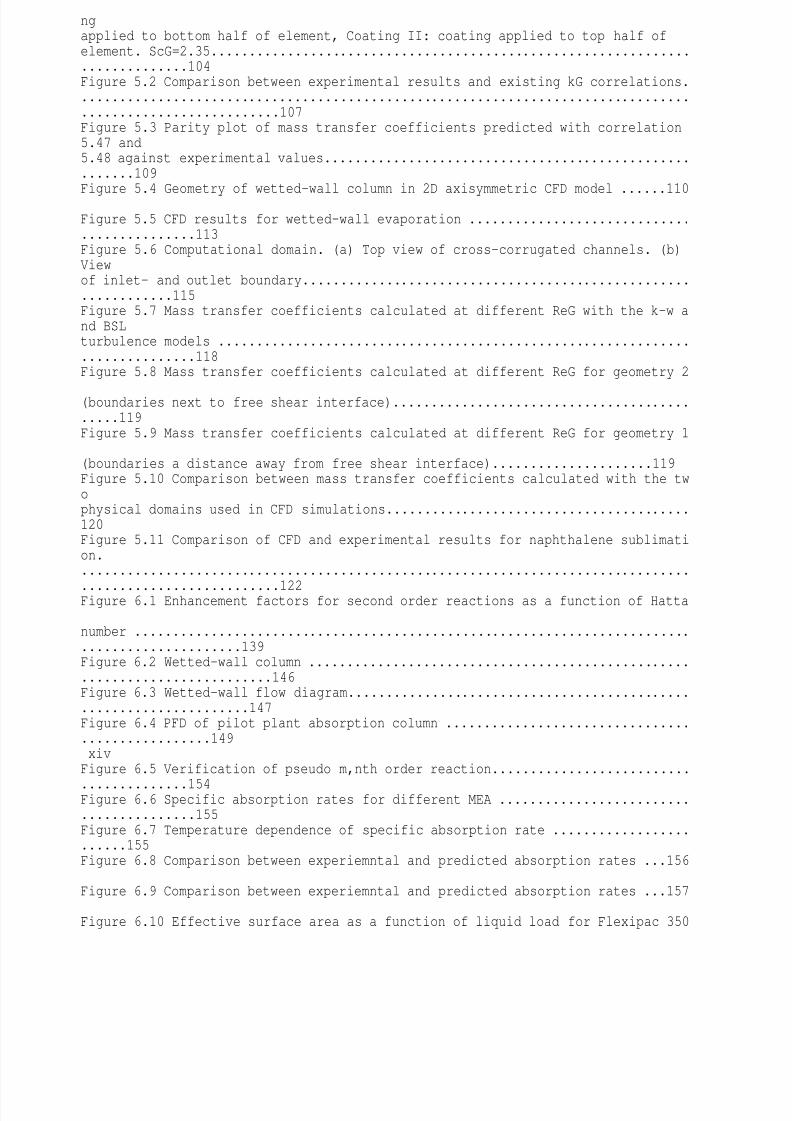
ngapplied to bottom half of element, Coating II: coating applied to top half ofelement. ScG=2.35.............................................................................104Figure 5.2 Comparison between experimental results and existing kG correlations...........................................................................................................107Figure 5.3 Parity plot of mass transfer coefficients predicted with correlation5.47 and5.48 against experimental values.......................................................109Figure 5.4 Geometry of wetted-wall column in 2D axisymmetric CFD model ......110 Figure 5.5 CFD results for wetted-wall evaporation ............................................113Figure 5.6 Computational domain. (a) Top view of cross-corrugated channels. (b)Viewof inlet- and outlet boundary...............................................................115Figure 5.7 Mass transfer coefficients calculated at different ReG with the k-w and BSLturbulence models .............................................................................118Figure 5.8 Mass transfer coefficients calculated at different ReG for geometry 2
(boundaries next to free shear interface)............................................119Figure 5.9 Mass transfer coefficients calculated at different ReG for geometry 1 (boundaries a distance away from free shear interface).....................119Figure 5.10 Comparison between mass transfer coefficients calculated with the twophysical domains used in CFD simulations........................................120Figure 5.11 Comparison of CFD and experimental results for naphthalene sublimation.................................................................................
..........................122Figure 6.1 Enhancement factors for second order reactions as a function of Hatta number ..............................................................................................139Figure 6.2 Wetted-wall column ...........................................................................146Figure 6.3 Wetted-wall flow diagram...................................................................147Figure 6.4 PFD of pilot plant absorption column .................................................149xivFigure 6.5 Verification of pseudo m,nth order reaction..........................
..............154Figure 6.6 Specific absorption rates for different MEA ........................................155Figure 6.7 Temperature dependence of specific absorption rate ........................155Figure 6.8 Comparison between experiemntal and predicted absorption rates ...156 Figure 6.9 Comparison between experiemntal and predicted absorption rates ...157 Figure 6.10 Effective surface area as a function of liquid load for Flexipac 350
8/10/2019 Erasmus Mass 2004.PDF
http://slidepdf.com/reader/full/erasmus-mass-2004pdf 11/257
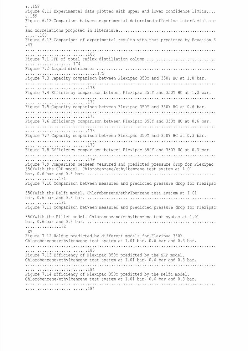
Y..158Figure 6.11 Experimental data plotted with upper and lower confidence limits......159Figure 6.12 Comparison between experimental determined effective interfacial areaand correlations proposed in literature...............................................160Figure 6.13 Comparison of experimental results with that predicted by Equation 6.47..........................................................................................................163Figure 7.1 PFD of total reflux distillation column .................................................174Figure 7.2 Liquid distributor ................................................................................175Figure 7.3 Capacity comparison between Flexipac 350Y and 350Y HC at 1.0 bar...........................................................................................................176Figure 7.4 Efficiency comparison between Flexipac 350Y and 350Y HC at 1.0 bar...........................................................................................................177Figure 7.5 Capacity comparison between Flexipac 350Y and 350Y HC at 0.6 bar...........................................................................................................177
Figure 7.6 Efficiency comparison between Flexipac 350Y and 350Y HC at 0.6 bar...........................................................................................................178Figure 7.7 Capacity comparison between Flexipac 350Y and 350Y HC at 0.3 bar...........................................................................................................178Figure 7.8 Efficiency comparison between Flexipac 350Y and 350Y HC at 0.3 bar...........................................................................................................179Figure 7.9 Comparison between measured and predicted pressure drop for Flexipac350Ywith the SRP model. Chlorobenzene/ethylbenzene test system at 1.01bar, 0.6 bar and 0.3 bar. ....................................................................181
Figure 7.10 Comparison between measured and predicted pressure drop for Flexipac 350Ywith the Delft model. Chlorobenzene/ethylbenzene test system at 1.01bar, 0.6 bar and 0.3 bar. ....................................................................181Figure 7.11 Comparison between measured and predicted pressure drop for Flexipac 350Ywith the Billet model. Chlorobenzene/ethylbenzene test system at 1.01bar, 0.6 bar and 0.3 bar. ....................................................................182xvFigure 7.12 Holdup predicted by different models for Flexipac 350Y.Chlorobenzene/ethylbenzene test system at 1.01 bar, 0.6 bar and 0.3 bar.
................................................................................
..........................183Figure 7.13 Efficiency of Flexipac 350Y predicted by the SRP model.Chlorobenzene/ethylbenzene test system at 1.01 bar, 0.6 bar and 0.3 bar...........................................................................................................184Figure 7.14 Efficiency of Flexipac 350Y predicted by the Delft model.Chlorobenzene/ethylbenzene test system at 1.01 bar, 0.6 bar and 0.3 bar...........................................................................................................184

8/10/2019 Erasmus Mass 2004.PDF
http://slidepdf.com/reader/full/erasmus-mass-2004pdf 12/257
Figure 7.15 Efficiency of Flexipac 350Y predicted by the Billet model.Chlorobenzene/ethylbenzene test system at 1.01 bar, 0.6 bar and 0.3 bar...........................................................................................................185Figure 7.16 Vapour phase mass transfer coefficient predictions by SRP, Delft and Billetmodels for Flexipac 350Y. Chlorobenzene/ethylbenzene test system at1.01 bar, 0.6 bar and 0.3 bar..............................................................186Figure 7.17 Liquid phase mass transfer coefficient predictions by SRP, Delft and Billetmodels for Flexipac 350Y. Chlorobenzene/ethylbenzene test system at1.01 bar, 0.6 bar and 0.3 bar..............................................................186Figure 7.18 Effective surface area predictions by SRP, Delft and Billet models forFlexipac 350Y. Chlorobenzene/ethylbenzene test system at 1.01 bar, 0.6bar and 0.3 bar. .................................................................................188Figure 7.19 Vapour phase mass transfer coefficient predicted with equation 5.48compared to predictions by SRP, Billet and Delft models.Chlorobenzene/ethylbenzene test system, 1.01 bar...........................189Figure 7.20 Effective surface area predicted with equation 6.47 compared to predictions
by SRP, Billet and Delft models. Chlorobenzene/ethylbenzene test system,total reflux, 1.01 bar. ..........................................................................190Figure 7.21 Efficiency of Flexipac 350Y predicted with kG and ae correlations developedin this study. Chlorobenzene/ethylbenzene test system at 1.01 bar, 0.6 barand 0.3 bar. .......................................................................................191Figure C.1 Pressure drop as function of F-factor for Flexipac 350Y, air/water system..........................................................................................................226Figure C.2 Holdup as function of F-factor for Flexipac 350Y, air/water system ..
.226xviFigure C.3 Pressure drop as function of F-factor for Flexipac 350Y, air/Kerosol200system ..............................................................................................227Figure C.4 Holdup as function of F-factor for Flexipac 350Y, air/Kerosol 200 system..........................................................................................................227Figure C.5 Pressure drop as function of F-factor for Flexipac 350Y HC, air/water system .........................................................................
.....................228Figure C.6 Holdup as function of F-factor for Flexipac 350Y HC, air/water system ..........................................................................................................228Figure C.7 Pressure drop as function of F-factor for Flexipac 350Y HC, air/Kerosol 200system ..............................................................................................229Figure C.8 Holdup as function of F-factor for Flexipac 350Y HC, air/Kerosol 200

8/10/2019 Erasmus Mass 2004.PDF
http://slidepdf.com/reader/full/erasmus-mass-2004pdf 13/257
system ..............................................................................................229
xviiLIST OF TABLES
Table 1.1 Examples from different generations of random packing......................4Table 1.2 Examples from different generations of structured packing ..................5Table 3.1 Formulas for the function f(|P|) .............................................................40Table 4.1 Physical properties of test system........................................................74Table 4.2 Dimensions of packing .........................................................................74Table 5.1 Dimensions of naphthalene coated packing section.............................103Table 5.2 Correlations for the gas phase mass transfer coefficient in Figure 5.2..106Table 5.3 Regression results for naphthalene sublimation data ...........................108Table 5.4 Boundary conditions: 2D axisymmetric wetted-wall model ...................111
Table 5.5 Mesh detail for 2D axisymmetric wetted-wall model .............................112Table 5.6 Properties of air/naphthalene system ...................................................114Table 5.7 Boundary conditions for micro element ................................................116Table 5.8 Details of converged grid for packing micro element ............................117Table 7.1 Constants for Flexipac 350Y used in the SRP model ...........................170Table 7.2 Constants for Flexipac 350Y used in the Delft model ...........................171Table 7.3 Constants for Flexipac 350Y used in the Billet model..................
.........171Table B.1 SRP model equations ..................................................
........................216Table B.2 Delft model equations ..........................................................................218Table B.3 Billet model equations..........................................................................220Table C.1 Experimental data for Flexipac 350Y, air/water system ........................230Table C.2 Experimental data for Flexipac 350Y, air/Kerosol 200 system..............233Table C.3 Experimental data for Flexipac 350Y HC, air/water system..................234
Table C.4 Experimental data for Flexipac 350Y HC, air/Kerosol 200 system........237Table D.1 Experimental sublimation data, bottom half of packing coated .............240Table D.2 Experimental sublimation data, top half of packing coated ...................241Table E.1 Physical properties of n-propanol.........................................................242Table E.2 Physical properties of monoethanolamine/n-propanol..........................242
8/10/2019 Erasmus Mass 2004.PDF
http://slidepdf.com/reader/full/erasmus-mass-2004pdf 14/257
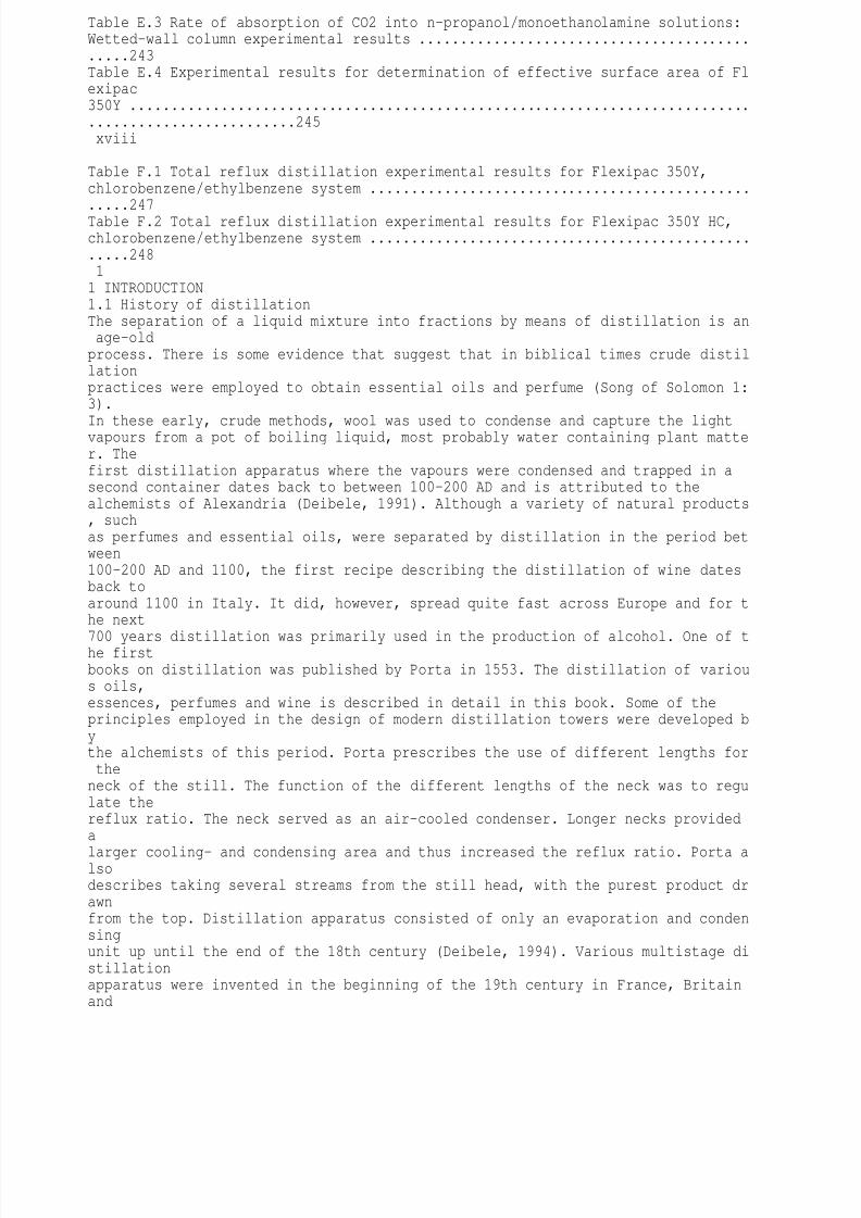
Table E.3 Rate of absorption of CO2 into n-propanol/monoethanolamine solutions:Wetted-wall column experimental results .............................................243Table E.4 Experimental results for determination of effective surface area of Flexipac350Y ....................................................................................................245xviii
Table F.1 Total reflux distillation experimental results for Flexipac 350Y,chlorobenzene/ethylbenzene system ...................................................247Table F.2 Total reflux distillation experimental results for Flexipac 350Y HC,chlorobenzene/ethylbenzene system ...................................................24811 INTRODUCTION1.1 History of distillationThe separation of a liquid mixture into fractions by means of distillation is an age-oldprocess. There is some evidence that suggest that in biblical times crude distillationpractices were employed to obtain essential oils and perfume (Song of Solomon 1:3).
In these early, crude methods, wool was used to condense and capture the lightvapours from a pot of boiling liquid, most probably water containing plant matter. Thefirst distillation apparatus where the vapours were condensed and trapped in asecond container dates back to between 100-200 AD and is attributed to thealchemists of Alexandria (Deibele, 1991). Although a variety of natural products, suchas perfumes and essential oils, were separated by distillation in the period between100-200 AD and 1100, the first recipe describing the distillation of wine datesback toaround 1100 in Italy. It did, however, spread quite fast across Europe and for the next
700 years distillation was primarily used in the production of alcohol. One of the firstbooks on distillation was published by Porta in 1553. The distillation of various oils,essences, perfumes and wine is described in detail in this book. Some of theprinciples employed in the design of modern distillation towers were developed bythe alchemists of this period. Porta prescribes the use of different lengths for theneck of the still. The function of the different lengths of the neck was to regulate thereflux ratio. The neck served as an air-cooled condenser. Longer necks provideda
larger cooling- and condensing area and thus increased the reflux ratio. Porta alsodescribes taking several streams from the still head, with the purest product drawnfrom the top. Distillation apparatus consisted of only an evaporation and condensingunit up until the end of the 18th century (Deibele, 1994). Various multistage distillationapparatus were invented in the beginning of the 19th century in France, Britainand

8/10/2019 Erasmus Mass 2004.PDF
http://slidepdf.com/reader/full/erasmus-mass-2004pdf 15/257
Germany. These apparatus were almost exclusively used in the production of alcoholfrom the various starting materials. In France wine was used as starting material, inEngland grain and in Germany potatoes. With some of these inventions it waspossible to obtain alcohol purities in excess of 90 vol%. The distillation column as weknow it today was invented in France in 1808 by Jean Baptiste Cellier-Blumenthal (Deibele, 1994). His column was equipped with an early form of the bubble cap trayand was used in the production of alcohol from wine. The first sieve tray column waspatented by Aenneas Coffey in England in 1832. Packing were used as far back as1830 when glass spheres were used in an alcohol still (Kister, 1992). During the 2beginning of the twentieth century the application of distillation spread rapidly fromalmost exclusively being used in the production of alcoholic beverages to the primaryseparation technique of liquid mixtures in the chemical industries. This rapidexpansion was largely due to the invention of petrol and diesel engines and thedemand for fuel. Distillation is presently still the primary method used for the
separation of liquid mixtures and with no technology set to replace it, will continue tobe so in future.1.2 Distillation and absorption todayThe oil and natural gas industry are by far the largest users of distillation andabsorption technology today. The size of the refining industry was estimated at3.7billion tonnes a year in 1991 and the amount of natural gas consumed in the same year in the order of 2000 billion m3 (Darton, 1992). The total distillation capacity of
refineries is estimated to exceed 5 billion tonnes a year. The natural gas industry isan important market for absorption technology since most of the natural gas istreated in absorption columns to remove water and acid gases. The petrochemicals sector is also a major user of distillation technology. In 1991 the global production ofolefins and aromatics were estimated to be around 130 million tonnes a year. Withouteven mentioning the use of distillation and absorption technology in the chemical andpharmaceutical industry, these figures show that distillation and absorption are
indeed a significant business area. Distillation and absorption are by no meansamature technology. Because of the shear size of the industry, small improvements inefficiency will result in large energy savings. It is estimated that by improving theestimation of the height equivalent to a theoretical plate, energy savings in the orderof 5% and capital savings in the order of 20% may be possible. Environmentallegislation and the global energy crisis in the 1970's and 1980's have stimulated

8/10/2019 Erasmus Mass 2004.PDF
http://slidepdf.com/reader/full/erasmus-mass-2004pdf 16/257
research into cheaper and more energy efficient distillation and absorptiontechnologies. This drive towards cheaper and more efficient processes has also leadto the combination of different unit operations in a single distillation column. Reactivedistillation has gained huge popularity in the past decade and a lot of research effortis focussed in this area. Another capital and energy saving development is thecombination of two columns in one shell, also referred to as the Petlyuk or dividedwall column. With this arrangement it is possible to obtain three product streams ofhigh purity from such a single column.
From the above figures and trends it is evident that distillation and absorption operations still pose huge challenges to the modern engineer. There is a constant3need for improving the efficiency and capacity of column internals. On the other handthere is a need for accurate models in order to be able to confidently design columnsthat will realize the improvements in efficiency and capacity of new column inte
rnalswithout resorting to huge design safety factors.1.3 Column internalsColumn internals may be classified as either trays or packing. The function of bothtrays and packing are to provide a large surface area for the vapour- and liquid phases to make contact with one another. When using trays, contact between vapourand liquid is established by bubbling the vapour through the liquid phase. The liquidphase is the continuous phase with the gas the dispersed phase. In packed columns
the packing provides a large surface area for the liquid to wet. The area between thevapour and liquid phases is provided by liquid films and drops. The vapour istherefore the continuous phase with the liquid the dispersed phase. Both trays andpacking are used extensively in modern distillation towers.1.3.1 TraysThere are a number of different types of trays commonly used in columns. They maybe broadly divided into bubble cap trays, sieve trays and valve trays. Most of theproprietary designs fall into one of these categories.
The bubble cap tray is the oldest design and has been the workhorse in columnsprior to 1960 (Kister, 1992). A bubble cap tray is a flat perforated plate withpipes(also called gas risers ) extending upwards from the perforations (holes). Caps arethe placed over the gas risers . These caps are equipped with slots and perforationsthrough which the vapour escapes to bubble through the liquid (hence the naming
bubble cap ). Compared to other trays they are expensive. They have a highturndown ratio but a low capacity. They are rarely used in modern towers.

8/10/2019 Erasmus Mass 2004.PDF
http://slidepdf.com/reader/full/erasmus-mass-2004pdf 17/257
The sieve tray is a simple design. It is basically a flat perforated plate without any`gas risers' or bubble caps. They are easy to fabricate and are therefore inexpensivecompared to other designs. They do however suffer from weeping (liquid flowingthrough the holes) and have a low turndown ratio.
A valve tray is also a flat perforated plate, but each perforation is equipped with amovable disk. At low vapour rates, these disks cover most of the open area andprevent the liquid from
weeping
. At larger vapour rates, the disks move vertically up4and expose more of the hole area. There is an upper limit on the movement of the disks determined by the length of the restrictive legs or the caging structure.Thereare a variety of proprietary designs for the perforations and the valves . Valve traysare frequently preferred above sieve trays because of their high turndown ratioandrelative small increase in cost.
The past decade has seen some major advances in tray design that have lead to an increase in both the hydraulic capacity and tray efficiency. The hydraulic capacity hasbeen increased by using multiple liquid downcomers. An example of such a designisthe VGMD tray and VortexTray from Sulzer Chemtech. The efficiency has beenincreased by using various valve- and aperture designs on valve- and sieve trays toincrease vapour/liquid contact and decrease dead volumes on trays.1.3.2 PackingPacking may be divided into three classes: Random packing
Structured packing GridsRandom packing was first developed followed by structured packing and grids.Random- and structured packing are widely used with grids being restricted to heattransfer applications and wash services (Kister, 1992). The following discussions willfocus on the development of random and structured packingRandom packingWith random packing, the packing elements are dumped into a column and form arandom structure for the liquid and vapour phases to pass through. These elementsare available in a wide variety of designs, sizes and materials. The development
ofrandom packing may historically be divided into three distinct phases. The differenttypes of random packing are therefore grouped into three generations. There arealarge number of proprietary designs. Some of the well known designs of the differentgenerations are given in table 1.1 (Kister, 1992). Each successive generationimproved on both the hydraulic capacity and the efficiency of the packing. Theimprovement from the second to the third generation was however less than from t

8/10/2019 Erasmus Mass 2004.PDF
http://slidepdf.com/reader/full/erasmus-mass-2004pdf 18/257
hefirst to the second generation of packing (Kister, 1992)
5Table 1.1 Examples from different generations of random packingFirst generation(1907-1950s)Second generation(1950s-1970s)Third generation(1970s-present)Raschig ringLessing ringBerl saddleIntalox saddleSuper Intalox packingPall ringHy-Pak packingIntalox metalCascade Mini-ringsLevapakNutter rings
FleximaxHiflow ringIntalox SnowflakeStructured packingThe need for packing with a high efficiency combined with an extremely low pressuredrop per theoretical stage lead to the development of packing with a regular orstructured geometry (Billet, 1995). Kister (Kister, 1992) describes the evolution ofstructured packing analogous to the evolution of random packing by classifying it intodifferent generations. The first two generations of structured packing weremanufactured from wire gauze. This type of packing was quite expensive compared
to random packing. They were mainly used in vacuum distillation applications wherea high number of theoretical stages were required combined with an extremely low pressure drop. The development of sheet metal structured packing (3rd generation ofstructured packing) by Sulzer in the late 1970's revolutionized the packing industry. Itmade structured packing more affordable and it became competitive withconventional internals (trays, random packing). The use of structured packing rose inpopularity to the point where it became the most popular column internal in useby
the end of the 1980's and early 1990's. The constant drive towards an increase incapacity has lead to some modifications being made to the third generation ofpacking in the late 1990's. These modifications have lead to an increase in capacitywith the same efficiency as the conventional third generation structured packing.Table 1.2 lists some of the well-known structured packing of the differentgenerations. A fourth generation of packing is included in the table. With two of thesepacking, namely Rombopak and Optiflow, there has been a move away from the
8/10/2019 Erasmus Mass 2004.PDF
http://slidepdf.com/reader/full/erasmus-mass-2004pdf 19/257
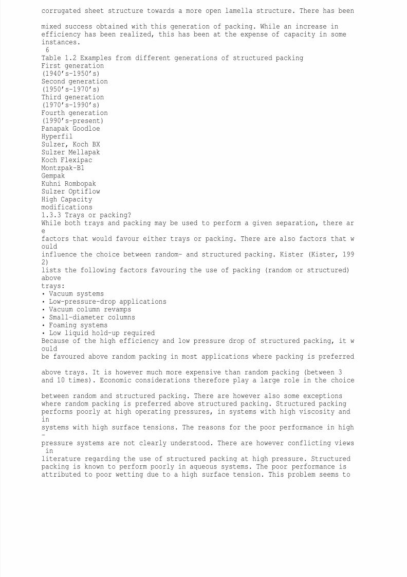
corrugated sheet structure towards a more open lamella structure. There has been mixed success obtained with this generation of packing. While an increase inefficiency has been realized, this has been at the expense of capacity in someinstances.6Table 1.2 Examples from different generations of structured packingFirst generation(1940's-1950's)Second generation(1950's-1970's)Third generation(1970's-1990's)Fourth generation(1990's-present)Panapak GoodloeHyperfilSulzer, Koch BXSulzer MellapakKoch FlexipacMontzpak-B1GempakKuhni RombopakSulzer Optiflow
High Capacitymodifications1.3.3 Trays or packing?While both trays and packing may be used to perform a given separation, there arefactors that would favour either trays or packing. There are also factors that wouldinfluence the choice between random- and structured packing. Kister (Kister, 1992)lists the following factors favouring the use of packing (random or structured)abovetrays: Vacuum systems
Low-pressure-drop applications Vacuum column revamps Small-diameter columns Foaming systems Low liquid hold-up requiredBecause of the high efficiency and low pressure drop of structured packing, it wouldbe favoured above random packing in most applications where packing is preferred above trays. It is however much more expensive than random packing (between 3and 10 times). Economic considerations therefore play a large role in the choice between random and structured packing. There are however also some exceptions
where random packing is preferred above structured packing. Structured packingperforms poorly at high operating pressures, in systems with high viscosity andinsystems with high surface tensions. The reasons for the poor performance in high-pressure systems are not clearly understood. There are however conflicting views inliterature regarding the use of structured packing at high pressure. Structuredpacking is known to perform poorly in aqueous systems. The poor performance isattributed to poor wetting due to a high surface tension. This problem seems to
8/10/2019 Erasmus Mass 2004.PDF
http://slidepdf.com/reader/full/erasmus-mass-2004pdf 20/257
bemost serious when stainless steel is used. The poor performance in systems withhigh viscosity is not fully understood yet. The older generations of structuredpackingalso performs poorly at high liquid loads, although it would seem that themodifications made to the third generation has improved this situation.7
There are situations where trays are favoured over packing. Kister, 1992, listssomeof these situations as: Solids present in feed High liquid rates Large diameter columns Complex columns Uncertainty in performance predictionMost of the arguments favouring the use of trays over packing presented by Kister(Kister, 1992) stem from practical considerations. Packing tends to become blockedwhen there is a large percentage of solids present in the feed or when coking or polymerisation occurs. Trays are favoured because they are easier to cleancompared to packing. In large diameter columns, good liquid and vapour distribut
ionbecomes essential to the efficient operation of both random and structured packing.Although efficient distributors are available for large diameter columns, it isoftenmore economical to use a tray column where mal-distribution of the phases is muchless of a problem. It is easier to accommodate heaters and coolers inside the columnshell when using trays compared to when using packing (complex columns). Highliquid rates may be accommodated in tray columns with the use of multi pass trays.These are all valid considerations favouring the use of trays over packing. What
is ofconcern though is when trays are favoured above packing because of the uncertaintyin predicting the performance of packing. The state of the art in predicting packingperformance is such that the same author (Kister, 1992) prefers rules of thumb anddata interpolation above semi theoretical models in predicting packing efficiency. Theproblem is also more severe with structured packing. This is probably because it hasnot been in use for as long a period as random packing. There have only beenrelatively few studies concerned with predicting structured packing efficiency.
1.4 Modelling of distillation and absorptionIn order to utilize the advantages that modern column internals offer, accuratemathematical models are needed to predict their efficiency and capacity.
For more than a century the equilibrium stage model has been used to modeldistillation and absorption equipment. The equilibrium stage model divides a columninto a number of stages where the liquid and vapour leaving such a stage are inthermodynamic equilibrium. In order to link these theoretical stages to real trays or

8/10/2019 Erasmus Mass 2004.PDF
http://slidepdf.com/reader/full/erasmus-mass-2004pdf 21/257
8beds of packing in columns, concepts like tray efficiencies and height equivalent to atheoretical plate (HETP) are introduced. While these concepts are adequate fordescribing binary systems, they are extremely confusing in multi component systems.In some circles it is believed that these concepts have severely retarded thedevelopment of distillation and absorption (Wesselingh, 1997).
The limitations of the equilibrium model in multi component and non-ideal systems,has lead to the development of the non-equilibrium model or rate-based approach(Krishnamurthy, 1985). With this modelling technique, thermodynamic equilibriumisonly assumed at the interface between the vapour and liquid phases. Rate equationsgovern the rate at which mass and heat are transferred from the interface to the bulkof the liquid and vapour phases leaving a non-equilibrium stage. Although this is animprovement on the equilibrium model, it is still not the exact model that engineersdream of.
The ideal `exact' model (Wesselingh, 1997) would be to subdivide the column into alarge number of sub domains (or grid) and solve the difference forms of theequations of fluid motion, diffusion and energy transfer on this computational grid.There are, however, still a few problems associated with doing this. The extremelylarge number of sub domains that would be necessary to adequately capture all theflow phenomena can not be accommodated by even the most advanced computeravailable at present. Even if this was the case, there is still a long way to go inunderstanding the physics governing multiphase, turbulent flow.
Since it is at present not possible to obtain an `exact' model, simplified hydraulic- andmass transfer models are needed in the equilibrium and non-equilibrium modelling approaches in order to predict the capacity and efficiency of column internals.Thereare a large number of correlations and semi-empirical models available in literatureon the capacity and efficiency of trays and random packing. Although structuredpacking offers significant capacity and efficiency advantages in some applications,there seems to be a lack of accurate efficiency models. It will also be shown that
some rather disturbing results are obtained with some of the efficiency modelspublished in the literature.1.5 Aims of this studyThis study focuses on the modelling of the capacity and efficiency of the sheetmetalstructured packing Flexipac 350Y, manufactured and marketed by Koch-Glitsch. Itis9a typical third generation structured packing. A modification has recently beenmade

8/10/2019 Erasmus Mass 2004.PDF
http://slidepdf.com/reader/full/erasmus-mass-2004pdf 22/257
to this packing that has lead to an increase in its capacity. At present this packingenjoys a fair portion of the market share with Koch-Glitsch performing at leastoneinstallation per week of the new high capacity version of Flexipac (Nieuwoudt,December 2003). There are, however, only a few mass transfer models available in literature to model the efficiency and capacity of sheet metal structured packing.Design engineers rarely trust these models and often resort to expensive pilot planttesting when designing a column containing structured packing. A major cause ofconcern in these mass transfer models is the accurate correlation of the vapourphase mass transfer coefficient and effective surface area. Correlations for thesequantities are often fitted on distillation data rather than measuring and correlatingthem independently. The primary objective of this study is therefore to developaccurate correlations for the vapour phase mass transfer coefficient and effectivesurface area. Accurate correlations will allow design engineers to use mass transfermodels with greater confidence and therefore save on time and money spent on pilot
plant testing. The aims of this study may be summarized as follows: Comparing results obtained with existing models in modelling the capacity ofFlexipac 350Y and identifying those more suitable. Measuring and correlating the vapour phase mass transfer coefficient forFlexipac 350Y independently from the effective surface area. Assessing the suitability of Computational Fluid Dynamics (CFD) in modellingthe vapour phase mass transfer coefficient in sheet metal structured packing. Measuring and correlating the effective interfacial area for vapour phasemass transfer for Flexipac 350Y independently from the vapour phase masstransfer coefficient. Comparing the results with existing efficiency and capacity models. Quantifying the performance of the high capacity packing in terms of capacityand efficiency and comparing it with the standard packing.
102 MODELLING OF DISTILLATION2.1 IntroductionThe equilibrium or stage based model has been used to model distillation columns for more than a century. The limitations of this approach have been recognized froman early stage. But, this approach is so simple and elegant from a mathematicalpointof view that it continues to be the primary method used in designing new distillation
columns. The recent advances made in the field of multicomponent mass transfercoupled with modern computing power and speed, have triggered the developmentof the so-called `non-equilibrium' or `rate-based' approach. It is fundamentally morecorrect than the equilibrium model. There is, however, a price to pay in terms ofcomplexity and computing resources. This chapter aims to introduce the different modelling approaches, and to highlight their strengths and weaknesses. Beforediscussing the different approaches, it is necessary to introduce basic concepts

8/10/2019 Erasmus Mass 2004.PDF
http://slidepdf.com/reader/full/erasmus-mass-2004pdf 23/257
regarding mass transfer across phase boundaries.2.2 Mass transfer across interfacesThe physical process that occurs inside a packed column is that of mass transfer across a vapour/liquid interface. The theory describing diffusional mass transfer inbinary systems is well developed (Cussler, 1984). Fick's Law is often used because of its simplicity and similarity to Fourier's Law for heat transfer (Incropera and DeWitt, 1990). In multicomponent mass transfer the Maxwell-Stefan relation fordiffusional mass transfer is used because it is generally less composition dependentcompared to the Fick diffusion coefficient (Taylor and Krishna, 1993). In the followingdiscussion on mass transfer across a phase boundary, the Maxwell-Stefan approach will be used. Only a brief review will be given. The literature should be consulted for amore complete discussion (Taylor and Krishna, 1993).2.2.1 Definition of mass transfer coefficientsIt is customary to define a mass transfer coefficient when estimating mass transferrates across a phase boundary. In order to avoid confusion, the mass transfer
coefficient in a binary system is defined in the same way as suggested by (Birdet al.,1960) and used by (Taylor and Krishna, 1993):( )1,b 1,b t 1,bb1 t 11,b 1,IN x N JlimitkN 0 c xx x-= =fi D- (2.1)]11The driving force is taken as the difference between the mole fraction of the
component in the bulk phase (x1,b) and the interface (x1,I). kb is expressed inunits of[m/s]. The mass transfer coefficient defined by Equation 2.1 is the zero flux masstransfer coefficient in terms of the bulk phase. For finite mass transfer rates, themass transfer coefficient is defined by:( )b1,b 1,b t 1,bt 11,b 1,IN x N Jkc xx x* -= =
D- (2.2)
The finite- (or high-) and zero flux coefficient are related through:b b bk k* = X (2.3)where Xb is the high flux correction factor. The mass transfer coefficient defined inEquation 2.1 (kb) corresponds to conditions of vanishing small mass transfer rates. Inreality, the velocity and composition profiles are distorted by the diffusion of

8/10/2019 Erasmus Mass 2004.PDF
http://slidepdf.com/reader/full/erasmus-mass-2004pdf 24/257
thespecies across the interface. The high flux correction factor (Xb) accounts forthisdistortion when calculating the high flux coefficient (kb*) from the zero flux coefficient(kb). Most mass transfer correlations are fitted on experimental data where themasstransfer rates are low. The zero flux coefficient is therefore obtained from thesecorrelations and should be corrected according to Equation 2.3 when used insituations where the mass transfer rate across an interface is high.
For a multicomponent system the diffusional flux is given by:( ) ( ) ( )( )b b tt bJ N x Nc k x*= -
= D (2.4)The high flux mass transfer coefficient is needed to determine the diffusional fluxes Jithat in turn are needed to determine the molar fluxes Ni. In order to determine
thediffusional fluxes and therefore the molar fluxes, we need to have methods fordetermining the low flux mass transfer coefficients and the high flux correction factors. A few models have been proposed to model the mass transfer across aphase boundary. The film model will be discussed in detail. A brief overview oftheremaining models will follow.122.2.2 Models for mass transfer at phase boundariesThe Film modelThe most common (and simplest) approach to modelling mass transfer acrossinterfaces is the well-known film theory proposed by Whitman (Whitman, 1923). Fr
oma mass transfer point of view the film model is attractive because of its simplicity. It isused more often than any of the other models. According to this model there exists astagnant layer of fluid next to the phase boundary through which mass transferoccurs by molecular diffusion alone. It is assumed that the level of turbulencein thebulk phase is high and will eliminate any concentration gradients. The concentrationgradient is confined to the stagnant layer next to the phase boundary. Krishna andStandart (Krishna and Standart, 1976) developed an exact solution to the Maxwell
-Stefan relations for the film model for an ideal gas mixture. For an ideal gas mixturethe Fick diffusion coefficient is constant and this is also a fair approximation fornonideal fluid mixtures where the change in concentration is small. The matrix of lowflux mass transfer coefficients is given by:[ ] [ ] 1k R -= (2.5)where
8/10/2019 Erasmus Mass 2004.PDF
http://slidepdf.com/reader/full/erasmus-mass-2004pdf 25/257
ni kiiin ikk 1k iij iij iny yR1 1R y=¹= +k k
= - - k k
(2.6)kij is the low flux mass transfer coefficient for the i-j binary pair and is defined by:k = ijij D
(2.7)If the diffusion fluxes are calculated at edge of the `film', the molar fractions used inEquation 2.4 are the bulk phase molar fractions. When the diffusion fluxes arecalculated at the interface the interface molar fractions are used. The high flu
xcorrection factors at the edge of the `film' and at the interface are given respectivelyby:[ ] [ ] [ ] [ ] 10 exp I - X = F F - (2.8)and[ ] [ ] [ ]0 expdX = X F (2.9)13[I] is the identy matrix and [F] is the rate factor matrix. The elements of therate factormatrix are calculated with:ni kii
t in t ikk 1k iij it ij t inN Nc c1 1Nc c=¹F = +k k
F = - - k k
(2.10)Assuming a constant D' along the diffusion path does not influence the molar fluxto asignificant extent (Taylor and Krishna, 1993). This assumption would lead to the useof average mole fractions in calculating [k] rather than boundary mole fractions. The
8/10/2019 Erasmus Mass 2004.PDF
http://slidepdf.com/reader/full/erasmus-mass-2004pdf 26/257
rate factor matrix [F] simplifies to [Y] with elements:ni,av t k,av tiit in t ikk 1k iij i,av tt ij t iny N y Nc c1 1y Nc c=¹Y = +k k
Y = - - k k
(2.11)For a non-ideal fluid system Krishna (Krishna, 1977) developed an approximatesolution by assuming that the thermodynamic rate factors Gik and Maxwell-Stefandiffusivity D'ik are constant along the diffusion path. The low flux mass transfer
coefficients are calculated with (using the appropriate molar fraction):[ ] [ ] [ ]1 avk R -= G (2.12)The elements of the matrix [R] are the same as in the ideal solution (Equation 2.6).The high flux correction factors are given by:[ ] [ ] [ ] [ ] 10 exp I - X = Q Q - (2.13)and[ ] [ ] [ ]0 expdX = X Q (2.14)where[ ] [ ] [ ]1av -Q = G F (2.15)[F] is the same as defined before.The binary low flux mass transfer coefficients are usually calculated from a mass
transfer correlation with the appropriate diffusivity. The molar fluxes (Ni) are neededin calculating the multi component low flux mass transfer coefficients and highfluxcorrection factors. An iterative scheme is therefore required in solving for Ni. Anumber of algorithms are given by Taylor and Krishna (Taylor and Krishna, 1993). 14Penetration theoryAccording to the penetration theory of Higbie the film next to the interface isconstantly replenished by eddies from the bulk of the fluid. These eddies stay at the
interface for a period of time. During this time mass transfer takes place normal to theinterface due to molecular diffusion (the eddies are static next to the interface). Theeddies then leave the interface to mix again with the bulk fluid. All eddies are assumed to stay at the interface for the same period of time. Equations for thelowflux mass transfer coefficients and high flux correction factors are presented by Bird

8/10/2019 Erasmus Mass 2004.PDF
http://slidepdf.com/reader/full/erasmus-mass-2004pdf 27/257
et al. (Bird et al., 1960) for binary systems and by Taylor and Krishna (TaylorandKrishna, 1993) for multicomponent systems. The penetration theory predicts themass transfer coefficient to be proportional to the square root of the diffusivity.Random surface renewal theoryDanckwerts (Danckwerts, 1951) refined the penetration theory by enforcing aresidence time distribution on the eddies at the interface. Mass transfer coefficientsand high flux correction factors for binary and multicomponent systems are given byTaylor and Krishna (Taylor and Krishna, 1993). This theory predicts the samedependence of the mass transfer coefficients on the diffusivity as the penetrationtheory.Film penetration theoryToor and Marchello (Toor and Marchello, 1958) showed that the film model and the penetration- and surface renewal models are complementary to each other and arelimiting cases of a more general solution. According to this general solution thepenetration- and surface renewal models will predominate in a developing boundarylayer while the film model will predominate in a fully developed boundary layer.
Between the two regions both mechanisms will contribute to the transfer process. Boundary layer theoryIn the boundary layer theory (Bird et al., 1960) allowance is made for a two-dimensional velocity profile. Transfer therefore occurs due to molecular diffusion in adirection normal to the interface and by convection parallel to the interface. Masstransfer coefficients and high flux correction factors are given by Bird et al.(Bird etal., 1960) in the form of plots for transfer from a flat surface to a laminar boundary
layer.15Turbulent mass transferIn turbulent flows there will be an extra contribution to the overall transfer process inthe form of turbulent eddies. A more detailed discussion of turbulence is giveninchapter 3.2.3 The Equilibrium Model2.3.1 Historical perspectiveThe first theoretical equations for continuous, steady state distillation were developedby Sorel in 1893. It was based on the concept of an equilibrium stage. These
equations formed the basis of the well known graphical solution methods: ThePonchon-Savarit method and the McCabe-Thiele construction. These methods werereplaced by rigorous computational methods when digital computers becameavailable. Numerous solution algorithms have been developed over the years(Naphtali and Sandholm, 1971) (Boston and Sullivan, 1972) (Tomich, 1970) (Wangand Henke, 1966) which have been implemented into commercially available process simulation software. It has been the subject of quite a few books (Henley andSeader, 1981, King, 1980, Holland, 1975).2.3.2 Model equations

8/10/2019 Erasmus Mass 2004.PDF
http://slidepdf.com/reader/full/erasmus-mass-2004pdf 28/257
In the equilibrium model the column is split up into a number of equilibrium stages (1to N stages). Figure 2.1 is a representation of an equilibrium stage (stage j).Thevapour and liquid leaving an equilibrium stage are assumed to be in thermodynamicequilibrium, i.e. there are no temperature difference and the mole fractions ofthecomponents in both phases correspond to their equilibrium values. Material andenergy balances are performed around each stage. These balances are collectively known as the `MESH' equations: M for material balances, E for equilibrium relations, S for summation equations and H for enthalpy balances (Henley and Seader, 1981,Holland, 1975, Foust et al., 1980).16UjWjQjVjyi,jTjHVjLj-1,
xi,j-1Tj-1HLj-1Vj+1yi,j+1Tj+1HVj+1Ljxi,jTjHLjFj, HFj
Figure 2.1 Stage j in equilibrium modelOverall material balance:( ) ( )t,j j 1 j 1 j j j j jM L V F L U V W 0- += + + - + - + = (2.16)Component balance:( ) ( )i,j j 1 i,j 1 j 1 i,j 1 j i,j j j i,j j j i,jM L x V y F z L U x V W y 0- - + += + + - + - + = (2.17)Equilibrium relations:i,j i,j i,j i,jE y K x 0= - = (2.18)Summation equations:( )cj ij iji 1S x y 0=
= - = (2.19)Enthalpy balances:( ) ( )L V F L Vj j 1 j 1 j 1 j 1 j j j j j j j j jH L H V H FH L U H V W H Q 0- - + += + + - + - + - = (2.20)Solution procedureIf there are c components in the system, 2c+3 equations have to be solved for eachstage. The 2c+3 variables are represented by a vector as:( ) ( )Tj j 1,j 2,j c,j j 1,j 2,j c,j jx V ,y ,y ,..,y ,T ,x ,x ,..,x ,L= (2.21)
8/10/2019 Erasmus Mass 2004.PDF
http://slidepdf.com/reader/full/erasmus-mass-2004pdf 29/257
The corresponding 2c+3 equations are represented by a vector as:( ) ( )Tj t,j 1,j 2,j c,j j 1,j 2,j c,j jF M ,M ,M ,..,M ,H ,E ,E ,..,E ,S= (2.22)17There are a vast number of iterative numerical methods and techniques used tosolve these equations. The most common methods are equation tearing proceduresand simultaneous correction procedures. The bubble point method (Wang andHenke, 1966) and sum-rates method are examples of the former class of methods.The Naphtali-Sandholm simultaneous correction method (Naphtali and Sandholm,1971) and the inside out method (Boston and Sullivan, 1972) are examples of thelatter class of procedures. In all the methods the well-known Thomas algorithm iswidely used because of the tridiagonal matrix form of the equations. Thesimultaneous correction procedures use a Newton Raphson method in conjunctionwith a matrix generalization of the Thomas algorithm. A detailed discussion of themethods and algorithms are beyond the scope of this text and can be foundelsewhere (Seader and Henley, 1998).2.3.3 Tray/stage efficiency in tray columnsThe method discussed above assumes that thermodynamic equilibrium is achievedbetween the liquid and vapour leaving a stage, with respect to both temperatureandcomposition. This assumption is acceptable for heat transfer in systems where the
temperature differences between stages are small. In most cases the assumption ofequilibrium between vapour- and liquid compositions are not reasonable. Thislimitation is overcome in tray columns by introducing stage- or tray efficiencies. Themethod proposed by Murphree is widely used. According to this method thecomponent K-value in equation 2.3, defined asi,ji,ji,jyKx= (2.23)are replaced with the Murphree vapour phase tray efficiency:
( ) i,j i,j 1MV i,ji,j i,j 1y yEy y+* +-=- (2.24)The equilibrium composition yi,j* is obtained from equation 2.6. The Murphreeefficiency is thus the ratio of the actual change in vapour phase composition to thechange that would have occurred if equilibrium were achieved. A measure of succe
sswas achieved in developing correlations for the Murphree efficiency and using it inbinary and ideal or near-ideal multicomponent systems. It has been demonstratedthat the Murphree efficiency varies widely from component to component and traytotray in non-ideal multicomponent mixtures, even becoming negative.182.3.4 Height equivalent to a theoretical plate (HETP) in packed columnsThe most common approach in evaluating the performance of packed columns in
8/10/2019 Erasmus Mass 2004.PDF
http://slidepdf.com/reader/full/erasmus-mass-2004pdf 30/257
distillation is in terms of the height equivalent to a theoretical plate, or HETP. Thismethod does not have any theoretical basis and is only used out of convenience.It isrelated to the height of packing needed for a specific separation by:eqzHETPN= (2.25)Neq is the number of equilibrium stages needed to model the separation performed ina real column with a packed height z.
2.4 Modelling distillation in packed columns: The HTU/NTUconcept2.4.1 Historical perspectiveThe packing in a packed column provides surface area for the continuous contactbetween the liquid and vapour phases. This is quite different from the stage conceptthat has been discussed up to this point. A method was proposed by Chilton andColburn (Chilton and Colburn, 1935) whereby the
HETP
concept is replaced by the
HTU
method. With this new method differential equations are integrated between the top and bottom compositions of the column to determine the height of packing
needed for a specific separation. At first it was assumed that the resistance to masstransfer is entirely in the vapour phase. The method was extended to account for resistance in both phases (Colburn, 1941). This method is still used extensively today, especially in the design of packed absorption columns (Sherwood et al., 1975,Seader and Henley, 1998, Foust et al., 1980, Henley and Seader, 1981, Holland,1975).2.4.2 Model equationsA mass balance is performed around a differential section of the tower (Foust et
al.,1980) (Figure 2.2):
19V1, y1V2, y2 L2, x2L1, x10z(V,y)z(V,y)z+dz (L,x)z+dz(L,x)zdz
Figure 2.2 Packed column with differential elementdV dL= (2.26)with the corresponding component balance given by:( ) ( )d Vy d Lx= (2.27)The rate of change of a component in a phase is equal to the rate at which thatcomponent is transferred to the phase. For equimolar counter diffusion the masstransfer rate for a component in the vapour phase can be expressed in terms of the

8/10/2019 Erasmus Mass 2004.PDF
http://slidepdf.com/reader/full/erasmus-mass-2004pdf 31/257
vapour phase mass transfer coefficient and the driving force:( ) ( )= -Gt G id Vy c k y y aSdz (2.28)where a is the interfacial area per unit volume of packing and S the cross sectionarea of the empty column. In this equation the flux correction factor has beenignored.It is more convenient to express the mass transfer rate in terms of the overallgasphase mass transfer coefficient:( ) ( )= -Gt OGd Vy c k y * y aSdz (2.29)y* is the mole fraction of the component corresponding to the concentration inequilibrium with the bulk liquid phase concentration. The vapour phase mass transfercoefficient (kG) and overall vapour phase mass transfer coefficient (kOG) is relatedthrough (Taylor and Krishna, 1993):= +GtOG LL Vtc m 1kk kc (2.30)20where m is the slope of the equilibrium curve.
Equation 2.12 may be used to solve the column height required by integratingbetween bottom and top compositions:( )( )21yzVt OG0 yd Vy1dzaS c k y * y= -

8/10/2019 Erasmus Mass 2004.PDF
http://slidepdf.com/reader/full/erasmus-mass-2004pdf 32/257

8/10/2019 Erasmus Mass 2004.PDF
http://slidepdf.com/reader/full/erasmus-mass-2004pdf 33/257
(2.31)If L and V are assumed constant over the length of the column and the physicalproperties do not vary appreciably so that a, ctV and kOG stay constant, equation 2.14simplifies to:( )( )= -=

8/10/2019 Erasmus Mass 2004.PDF
http://slidepdf.com/reader/full/erasmus-mass-2004pdf 34/257
21yGt OGyT,OG T,OGd yVzy * yaSc kH N (2.32)The quantity outside the integral is called the `height of a transfer unit' (HT) while theintegral term is called the `number of transfer units' (NT). The driving force and masstransfer coefficients used in this equation are based on the bulk vapour phase andare indicated by the subscript (OG). An approximation of the integral term, or numberof transfer units (NT,OG) is given by:( )( )2 1T,OG LMy yNy y*
-=- (2.33)where( ) ( ) ( )( )( )2 2 1 1LM 2 21 1y y y yy yy yln
y y* ****- - -- =-- (2.34)If the slope of the equilibrium line is constant, then this approximation simplifies to:( )
( )T,OGVln K LN VK 1L=- (2.35)In distillation the assumption of constant L and V is only true for equimolar transferand for columns operated under conditions of total reflux. If the method is to b
8/10/2019 Erasmus Mass 2004.PDF
http://slidepdf.com/reader/full/erasmus-mass-2004pdf 35/257
e usedfor packed distillation columns in general, then the simplifications introducedbyassuming constant L and V and constant properties cannot be made and equation2.29 has to be integrated over the height of the column, or at least separatelyfor therectification- and stripping sections. The method is, however, widely applied to anequilibrium stage where the assumptions do apply (Sherwood et al., 1975). The21height of packing determined in this way is simply the HETP. A summation of theHETP's over all the equilibrium stages give the total height of packing. An extensionof the method using multicomponent mass transfer theory is giving by Taylor andKrishna (Taylor and Krishna, 1993).2.5 The Non-equilibrium Model2.5.1 Historical perspectiveReal stages in a distillation column rarely operate at equilibrium conditions. Stage- ortray efficiencies were introduced into the equilibrium model to account for this departure from equilibrium. The Murphree efficiency described previously is oneofmany such definitions. For a multicomponent mixture containing c components, the
reare c-1 independent component efficiencies. These efficiencies are usually taken tobe equal to one another. A wide body of evidence suggested that this is not true (Krishna et al., 1977, Vogelpohl, 1979). This is because in multicomponent mixturesthe diffusion of different species is coupled with one another. Models that account forthese interaction effects became available (Krishna and Standart, 1979). At firstthese models were used to estimate efficiencies in multicomponent systems(Vogelpohl, 1979). These models were, however, quite complicated. A new modellin
gapproach was suggested (Krishnamurthy and Taylor, 1985a) where themulticomponent mass transfer models are used directly instead of in the form oftrayefficiencies. The model was tested against binary and multicomponent distillationdata, and found to yield satisfactory results (Krishnamurthy and Taylor, 1985b). Itwas also compared with the equilibrium stage model (with tray efficiencies) andfound to be superior (Krishnamurthy and Taylor, 1985c). This model is called the non-equilibrium model or rate-based approach and will be discussed in more detail in
the next paragraph. Since its inception there has been various modifications and extensions. The solution algorithm was improved (Powers et al., 1988) and the modelwas extended to include pressure as a variable and to account for weeping andentrainment in plate columns (Taylor et al., 1994). It has also been used to modelreactive separation processes (Higler et al., 1998, Higler et al., 1999a, Higler et al.,1999b).

8/10/2019 Erasmus Mass 2004.PDF
http://slidepdf.com/reader/full/erasmus-mass-2004pdf 36/257
2.5.2 Model equationsIn the non-equilibrium model the column is again split up into a number of stages (1to N). Phase equilibrium is only assumed at the interface between two adjoiningphases. This is fundamentally different from the equilibrium approach where22thermodynamic equilibrium is assumed between the liquid and vapour leaving astage. In the non-equilibrium model, separate material- and energy balances areperformed for each phase. These balances are linked by mass- and energy transfer across the interface. Collectively the equations for the non-equilibrium model areknown as the `MERSHQ' equations: M for material balances, E for energy balances,R for transfer rate equations, S for summation equations, H for hydraulic equationsand Q for equilibrium equations. Figure 2.3 represents stage j in the non-equilibriummodelVj+1yi,j+1TVj+1HVj+1UjWj
QjLQjVfLi,j, HLFjLj-1,xi,j-1TLj-1HLj-1Vjyi,jTVjHVjLjxi,jTLj
HLjfVi,j, HVFj NjEj Figure 2.3 Stage j in non-equilibrium modelConservation equations for the vapour phase:Component material balance for species i in the vapour phase:( ) + += + - - + N =V V Vi,j j j i,j j 1 i,j 1 i,j i,jM V W y V y f 0 (2.36)where fi,jV is the vapour feed flow rate of component i on stage j.Overall material balance for the vapour phase:+= - - + + N =V V Vt,j j j 1 j j t,jM V V F W 0 (2.37)where FjV is the total vapour feed flow rate to stage j.Energy balance for the vapour phase:
( ) + += + - - + + E =V V V V VF V Vj j j j j 1 j 1 j j j jE V W H V H F H Q 0(2.38)Conservation equations for the liquid phase:23Component material balance for species i in the liquid phase:( ) + += + - - - N =L L Li,j j j i,j j 1 i,j 1 i,j i,jM L U x L x f 0 (2.39)where fi,jL is the liquid feed flow rate of component i on stage j.Overall material balance for the liquid phase:+= - - + - N =L L Lt,j j j 1 j j t,jM L L F U 0 (2.40)where FjL is the total liquid feed flow rate to stage j.

8/10/2019 Erasmus Mass 2004.PDF
http://slidepdf.com/reader/full/erasmus-mass-2004pdf 37/257
Energy balance for the liquid phase:( ) + += + - - - E =L L L L LF L Lj j j j j 1 j 1 j j j jE L U H L H F H Q 0 (2.41)Conservation equations for the interface:There is no accumulation of material at the interface:= N - N =I V Li,j i,j i,jM 0 (2.42)An energy balance performed around the interface yields:= E - E =I V Lj j jE 0 (2.43)Equilibrium equationsEquilibrium between vapour and liquid is assumed at the interface:I I Ii,j i,j i,j i,jQ K x y 0= - = (2.44)In addition the mole fractions at the interface should sum to unity:cVI Ij i,ji 1S y 1 0== - = (2.45)cLI Ij i,ji 1S x 1 0== - = (2.46)
Hydraulic equationWith the pressure on the first (top) stage specified, the pressure across the columncould be calculated from a suitable model. The pressure on stage j is calculated from:( )j j j 1 j 1P P P P 0- -= - - D = (2.47)Rate equationsThe total mass transfer rate for the vapour phase is given by:( ) ( ) ( ) N = X - + N V V V V I Vj t,j j j j j j t,j jc k a y y y (2.48)and for the liquid phase:24( ) ( ) ( ) N = X - + N L L L L I Lj t,j j j j j j t,j jc k a x x x (2.49)
[kjV] and [kjL] are the matrices of multicomponent low flux mass transfer equations.The energy transfer rate for the vapour phase is obtained from:( )=E = - + N c VV V V Ii,jj j j j j i,ji 1h a T T H (2.50)The energy transfer rate for the liquid phase is obtained from:( )=
E = - + N c LL L I Li,jj j j j j i,ji 1h a T T H (2.51)Reduction in number of variablesA reduction in the total number of unknown variables is possible because only oneset of mass transfer rates is independent:N = N = NV Li,j i,j i,j (2.52)
8/10/2019 Erasmus Mass 2004.PDF
http://slidepdf.com/reader/full/erasmus-mass-2004pdf 38/257
The mass transfer rates for the vapour and liquid phases in Equations 2.36 and 2.39are replaced with Ni,j and the mass transfer rates (Equations 2.48 and 2.49) are combined with the interface material balances (Equation 2.42) to give:= N - N =i,jV Vi,j i,jR 0 (2.53)where ( )=N = NV V I Vi,j ik,j j k,j k,j k,jk 1,2,..,cf k ,a ,y ,y , (2.54)and= N - N =i,jL Li,j i,jR 0 (2.55)where ( )=N = NL L I Li,j ik,j j k,j k,j k,jk 1,2,..,cf k ,a ,x ,x , (2.56)Only c-1 of these equations are independent. The mass transfer rate for the last
component is implicit in the energy balances. The energy transfer rates (Equations2.50 and 2.51) are combined with the interface energy balance (Equation 2.43) to give:( ) ( )=
= - - - + N - =
c V LI V V I L I Li,j i,jj j j j j j j j j i,ji 1
E h a T T h a T T H H 0 (2.57)Solution procedureThe 5c+6 variables for each stage are represented by a vector as:25( ) ()=N N NT V I I I I I I Ij j 1,j 2,j c,j j 1,j 2,j c,j 1,j 2,j c,j j jL1,j 2,j c,j j 1,j 2,j c,j jx V ,y ,y ,..,y ,T ,y ,y ,..,y ,x ,x ,..,x ,T ,L ,x ,x ,..,x ,T , , ,.., ,P
(2.58)The corresponding 5c+6 equations are represented by a vector as:( ) ()T V V V V V V V V VI I I I Ij t,j 1,j 2,j c,j j 1,j 2,j c 1,j j 1,j 2,j c,j jL L L L L L L L LIt,j 1,j 2,j c,j j 1,j 2,j c 1,j j jF M ,M ,M ,..,M ,E ,R ,R ,..,R ,S ,Q ,Q ,..,Q ,E ,M ,M ,M ,..,M ,E ,R ,R ,..,R ,S ,P-

8/10/2019 Erasmus Mass 2004.PDF
http://slidepdf.com/reader/full/erasmus-mass-2004pdf 39/257
-= (2.59)The condenser and reboiler in a non-equilibrium model are modelled as equilibriumstages. Simultaneous correction methods are widely used to solve the set of non-linear equations (Taylor and Krishna, 1993, Krishnamurthy and Taylor, 1985a). Whenusing a simultaneous correction method, it is necessary to supply an initial estimatefor all the variables. It is important that these initial estimates are sensible in the caseof the non-equilibrium model. Incorporated into the model are models (empiricalandfundamental) for mass transfer coefficients and pressure drop. Initial estimates outside the physical bounds of these `closure' models will cause the non-equilibrium model to diverge. Because of pressure being included as a variable, a computationalpenalty is added in the evaluation of partial derivatives of all the equations withrespect to pressure (especially the thermodynamic properties). Although there ar
equite a few more equations per stage to solve, and the added complexity of obtainingpartial derivatives of equations with respect to pressure, a non-equilibrium model isabout as difficult to converge as its equilibrium counterpart (Krishnamurthy and Taylor, 1985a) The computational effort is further reduced if the high flux correctionfactors are omitted. They were found not to be important in distillation (Powers et al.,1988).2.6 Concluding remarks
Despite its weaknesses and lack of any theoretical basis, the HETP concept is stillwidely used in the design of columns containing structured packing. When using thisconcept one often has to resort to expensive and time consuming pilot plant testing.This could impact the economics of a process negatively. In this chapter thealternative modelling approaches have been introduced and discussed. Thesemodelling approaches are not new and have been around for some time. TheHTU/NTU method were introduced in the 1930 s and the rate-based approach in the1980 s. In order to use the advantages that these modelling approaches offer,accurate hydrodynamic- and mass transfer models are needed. The current state of
26affairs is such that a leading authority on distillation still views the use ofmasstransfer models as the least accurate method to determine the height of packingfor agiven separation (Kister, 1992).
The chapters that follow aim to introduce and critically assess the hydrodynamic- andmass transfer models available in literature. Inaccurate correlations for the va

8/10/2019 Erasmus Mass 2004.PDF
http://slidepdf.com/reader/full/erasmus-mass-2004pdf 40/257
pourphase mass transfer coefficient and effective surface area were identified asweaknesses in current available mass transfer models. Experimental- and modellingtechniques are employed to develop more accurate correlations for these quantities.272.7 Nomenclaturea Effective surface area of packing [m2/m3]c Molar density [mol/m3]D Fick diffusion coefficient [m2/s]D
Maxwell-Stefan diffusion coefficient [m2/s]E Energy transfer rate [W]F Feed molar flow rate [mol/s]H Enthalpy [J/mol]h Heat transfer coefficient [W/(m2 K)]H Partial specific enthalpy [J/mol]HETP Height equivalent to a theoretical plate [m]HT Height of a transfer unit [m]J Diffusional flux [mol/(m2 s)]K Equilibrium constant [--]k Low flux mass transfer coefficient [m/s]k* Finite flux mass transfer coefficient [m/s]L Liquid molar flow rate [mol/s]
Film thickness [m]N Molar flux [mol/(m2 s)]N Molar transfer rate [mol/s]Neq Number of equilibrium stages [-]NT Number of transfer units [-]P Pressure [Pa]Q Heat duty [W]S Column cross sectional area [m2]T Temperature [K]U Liquid side draw molar flow rate [mol/s]V Vapour molar flow rate [mol/s]W Vapour side draw molar flow rate [mol/s]x Mole fraction, liquid phase [-]
y Mole fraction, vapour phase [-]z Height of packing [m]GreekG Thermodynamic rate factors [-]28d Kronecker delta [-]d Distance from interface [m]g Liquid activity coefficient [-]X High flux correction factor [-]kij Low flux i-j pair binary mass transfer coefficient [m/s]F Rate factors [-]Y Rate factors assuming constant D
[-]Q Rate factors for mass transfer in non-ideal fluids [-]
Subscriptsav Average propertyi,j,k Component indicesL Liquid phase propertyOL Overall liquid phase propertyOG Overall vapour phase propertyt Refers to the total mixtureG Vapour phase propertySuperscriptF Feed property

8/10/2019 Erasmus Mass 2004.PDF
http://slidepdf.com/reader/full/erasmus-mass-2004pdf 41/257
I Interface propertyL Liquid phase propertyV Vapour phase property
293 CFD AND STRUCTURED PACKING3.1 IntroductionComputational Fluid Dynamics (CFD) is now an established modelling tool in thechemical process industry. This is to a large extent due to the advances made in computational speed and improvements in physical models implemented into CFD.There are already plans to combine CFD with traditional process simulation softwarein order to make it accessible to the average chemical engineer (Shanley, 2000). Themajor advantage of CFD is that it reduces the amount of physical testing that has tobe performed and therefore reduces overall development costs. There are howeverlimitations to what CFD can do and this should always be kept in mind. Theselimitations usually manifest itself in two ways. The first is that current modelsavailable in CFD may not be able to accurately model the physical process. Secondly
the physical domain may be too large and complex to be represented by a CFDmodel. In the current study both these limitations are encountered. In a packeddistillation column one is faced with stratified counter current two phase flowthrougha complex geometry. Only elementary physical models are available for this typeofflow. It would also be impossible to model a whole segment of packing, let alone thewhole column. In order to use the advantages that CFD offers, some simplificationshave to be made. This chapter will look at how CFD has been used in the past inthestructured packing industry and how it was implemented in this study.
3.2 Literature review3.2.1 Application of CFD in the structured packing industryCFD technology has been used in the past in the optimisation of structured packingdesigns. Mention is sometimes made of the use of CFD in optimising designs insome packing vendor brochures. These results are certainly of a proprietary natureand therefore not published in the open literature. There are however a few studiesthat have been conducted at universities for which results are available. In most ofthese studies only single-phase flow is assumed. Some of the studies werespecifically on structured packing while others focussed on applications where
geometries similar to that of structured packing are employed. These applicationsgenerally involve heat transfer. A short review of these follows.
30Probably the first published CFD study on a geometry quite similar to that found incorrugated structured packing, is the study by Ciofalo and co-workers (Ciofalo et al.,1996), (Ciofalo, 1996). The study was performed on a type of compact heat

8/10/2019 Erasmus Mass 2004.PDF
http://slidepdf.com/reader/full/erasmus-mass-2004pdf 42/257
exchanger called a rotary regenerator. This heat exchanger is made of a matrix ofclosely packed corrugated steel plates, quite similar to the corrugated geometry ofmost commercial structured packing (Mellapak, Flexipac). The heat transfer andpressure drop occurring in a unitary cell in the corrugated matrix were modelled usingan early release of the software used in this study (FLOW3D). The results obtainedwith different turbulence models were compared with experimental data. The lowReynolds number formulation of the k-e model and LES (large eddy simulation) gavethe best overall agreement compared to experimental data.
The motivation behind the study of Hodson (Hodson, 1997) (Hodson et al., 1997)was to modify the existing geometry of corrugated sheet structured packing in orderto maximize the gas phase mass transfer rate. The study was not concerned withpredicting the gas phase mass transfer rate, but rather to compare qualitatively different modifications to the standard design. The standard k-e model was usedwitha wall function to bridge the laminar sublayer. A single unitary cell was modelled and
the outflow used as inflow to a next cell. A layer of packing was modelled bystaggering a number of these cells. Heat transfer from the wall as well as pressuredrop was modelled. A modification to the standard design was proposed. Thismodification involved punching slots into the corrugated sheets with the punched outtabs protruding into neighbouring channels. A sample of the modified packing was produced and tested. The separation efficiency of the packing was marginallyincreased. This was however at the expense of capacity.
The dry pressure drop over structured packing is used in most of the proposedpressure drop models. CFD has recently been successfully used to predict the dry
pressure drop of most commercially available structured packing (Petre et al., 2003).The study was also extended to the dry pressure drop through the modern
highcapacity structured packing (Larachi et al., 2003). In the study, the total pressuredrop is divided into different contributing mechanism. Each mechanism is modelledseparately and then combined according to the model proposed by Olujic (Olujic,1997). The k-e turbulence model with a wall function was used in the study.
31A successful attempt has been made at using CFD to model binary distillation in
abed of random packing (Yin et al., 2000). The packed bed is modelled as a twodimensional porous region and existing correlations are used for quantities like pressure drop, hold-up and mass transfer coefficients. The results comparedfavourably with experimental results obtained from the FRI.
The radial and axial dispersion of the liquid phase in structured packing developedfor catalytic distillation (KATAPAK-S) (Van Baten et al., 2001) has been modelle
8/10/2019 Erasmus Mass 2004.PDF
http://slidepdf.com/reader/full/erasmus-mass-2004pdf 43/257
dwith CFD. Good agreement was obtained with experimental data.
Vapour flow around some of the other internals found in packed columns has alsobeen the subject of a few CFD studies. These include the modelling of reboilervapour return lines (Wehrli et al., 2002) and the maldistribution of the vapourphasecaused by liquid redistributors (Mohamed Ali et al., 2002). In these studies the k-eturbulence model with a wall function were used. CFD has also been used in a studyon liquid film flow on inclined plates (Ataki and Bart, 2002).
The use of CFD is not only confined to structured packing. It has also been used tomodel sieve tray hydrodynamics (Krishna et al., 1999) and the flow inside liquid-liquidextractors (Rieger et al., 1996).3.2.2 Aim of CFD in this studyCFD has previously successfully been used to model mass transfer rates in complexwall bounded flows (Nesic and Postlethwaite, 1992, Nesic et al., 1993, Wang andShirazi, 2001). It has also been demonstrated that CFD can be successfully usedto
model the vapour phase flow in structured packing (Larachi et al., 2003, Petre et al.,2003, Hodson, 1997). A natural extension of these ideas would be to use CFD tomodel the vapour phase mass transfer in structured packing. This was the mainfocus of the CFD work in this study. In the remainder of this chapter the generalmodelling philosophy will be presented. It will start with an overview of the governingequations of fluid flow and how these equations are approximated with the use of computational fluid dynamics. The main features of the CFD code used in this studywill be introduced. Finally some details will be given on how CFD was implemente
d inthis study. Chapter 5 should be consulted for a more detailed description of the geometry and boundary conditions used in implementing CFD in this study.323.3 Theory: Computational fluid dynamicsThe governing equations describing the motion of a fluid are complex and highlynon-linear. Analytical methods for solving these equations are limited to only the mostelementary problems. In computational fluid dynamics (or CFD in short) thegoverning equations are approximated with a suitable discretization method. Theequations are expressed in terms of a set of algebraic equations for the discret
evariables at a set of discrete locations in the computational space. Variousdiscretization methods have been developed over the years. Methods that arefrequently used are the finite element method, the finite difference method andthefinite volume method. Most CFD codes use the finite volume method. This is alsothecase with CFX-4, the commercial package used in this study. In the paragraphs thatfollow the conservation equations will be discussed, followed by the discretizat
8/10/2019 Erasmus Mass 2004.PDF
http://slidepdf.com/reader/full/erasmus-mass-2004pdf 44/257
ionmethod and finally the solution procedure. The discretization method that will bediscussed is the finite volume method. Discretization methods for the finite differenceand finite element methods can be found elsewhere.(Patankar, 1980)3.3.1 Conservation equationsThe Navier-Stokes equationsThe conservation equation for mass over a stationary volume element through whicha fluid flows is known as the continuity equation. In a three dimensional cartesiancoordinate frame it is represented by (Schlichting, 1979):x y zU U U 0t x y z
¶r ¶ ¶ ¶+ r + r + r = ¶ ¶ ¶ ¶ (3.1)The conservation equations for momentum in Newtonian fluids in a three dimensionalcartesian coordinate frame are given by (Schlichting, 1979):( )x x x y x z xxx yx zx xU U U U U U Ut x y zp gx x y z
¶ ¶ ¶ ¶r + r + r + r ¶ ¶ ¶ ¶ ¶ ¶ ¶ ¶= - - t + t + t + r ¶ ¶ ¶ ¶ (3.2)( )y x y y y z yxy yy zy yU U U U U U Ut x y zp gy x y z
¶ ¶ ¶ ¶r + r + r + r ¶ ¶ ¶ ¶ ¶ ¶ ¶ ¶= - - t + t + t + r
¶ ¶ ¶ ¶ (3.3)33( )z x z y z z zxz yz zz zU U U U U U Ut x y zp gz x y z
¶ ¶ ¶ ¶r + r + r + r ¶ ¶ ¶ ¶ ¶ ¶ ¶ ¶= - - t + t + t + r ¶ ¶ ¶ ¶ (3.4)
The expressions for the stress terms are:( )U+¶¶m-=t 32xU2 xxx (3.5)( )U+¶¶-= 32yU2 yyy mt (3.6)( )U+¶¶m-=t 32zU2 zzz (3.7)yxxy yxUUy x¶ ¶t = t = -m +
¶ 
8/10/2019 Erasmus Mass 2004.PDF
http://slidepdf.com/reader/full/erasmus-mass-2004pdf 45/257
(3.8)y zyz zyU Uz y¶ ¶t = t = -m +
¶ ¶ (3.9)z xzx xz U Ux z¶ ¶ t = t = -m +
¶ ¶ (3.10)It is convenient to write the continuity equation in vector notation:( ) 0t =r+¶r¶ U (3.11)In vector notation the momentum balances are represented by:( ) ( ) gUUU r+--=Är+r¶¶ t pt (3.12)The above equations are known as the Navier-Stokes equations. They completelydescribe the flow of an isothermal Newtonian fluid.General conservation equationA general convection-diffusion conservation equation may by written that governs momentum, mass and heat transfer (Patankar, 1980):
( ) ( ) ( ) ff +f G=fr+rf¶¶ St U (3.13)In this equation f is the dependent variable, Gf is the diffusion coefficient and Sf isthe source term. The source term represents the creation or destruction of thedependent variable. For the simple example of conduction, f would representtemperature, Gf the thermal conductivity and Sf some external heat source. Forthe34momentum equation (Equation 3.12), f represents the velocity vector and Gfrepresents viscosity . A number of quantities are lumped into the source term, Sf . Itcontains the pressure gradient, body forces such as gravitation and a part of the
stress term.TurbulenceIn most engineering problems turbulent flows are encountered. Turbulence is still anactive area of research and there is a large amount of literature devoted to it. Fundamentally, the Navier-Stokes equations also apply to turbulent flows. It ispossible to use these equations directly to simulate turbulent flow. This is called
Direct Numerical Simulation . It is currently possible to model only simple turbulentflows with this method and even then extensive computational resources are needed
(Hirsch, 1988). Most of the models in use today rely on the Reynolds averagedNavier Stokes equations. With this method the turbulent fluctuations are averagedout. This gives rise to mean or time averaged turbulence quantities. The time overwhich this averaging is carried out must be sufficiently large compared to the timescale of the turbulent fluctuations but sufficiently small compared to the timescale ofother time dependent phenomena. The time-averaged component of velocity in the x
8/10/2019 Erasmus Mass 2004.PDF
http://slidepdf.com/reader/full/erasmus-mass-2004pdf 46/257
direction is given by (Schlichting, 1979):0t+tx xt01U U dtt= (3.14)The instantaneous velocity is then the sum of the time averaged velocity and avelocity fluctuation:xx xU U U= + (3.15)Similar expressions apply to the other components of velocity and any othertransported quantity in general. The Navier-Stokes equations are rewritten in terms ofthese quantities. In Cartesian coordinates the continuity equation is given by:x y zU U U 0t x y z
¶r ¶ ¶ ¶+ r + r + r = ¶ ¶ ¶ ¶ (3.16)The momentum equation in the x direction is represented by:( )x x x y x z x2 xx x y x z x xU U U U U U Ut x y zp U U U U U U U gx x y z
¶ ¶ ¶ ¶r + r + r + r
¶ ¶ ¶ ¶ ¶ ¶ ¶ ¶= - - r + r + r + m + r ¶ ¶ ¶ ¶ (3.17)Similar expressions can be written for the y and z components of the momentumequation. The terms35txx x xU U t = r tyx y xU U t = r tzx z xU U t = r (3.18)are known as the Reynolds stresses. Various models have been proposed tocalculate these stresses. Most models rely on Boussinesq s eddy viscosityhypothesis, analogous to Newton s law of viscosity:xtyx t
dUdyt = -m (3.19)were mt is the turbulent- or eddy viscosity. Similar averaging may be performedonthe general convection-diffusion equation. The eddy diffusivity hypothesis is theresult. The turbulent transport of quantities like heat and mass are due to thesamemechanism as momentum transport. It is therefore expected that the value of theeddy diffusivity will be close or equal to that of the eddy viscosity. This hasresulted inthe definition of turbulent Prandtl/Schmidt numbers:t
ttffms =G (3.20)Quite a few turbulence models have been proposed that rely on the eddy viscosity concept. These models can be divided into one- and two equation models. The k-e

8/10/2019 Erasmus Mass 2004.PDF
http://slidepdf.com/reader/full/erasmus-mass-2004pdf 47/257
model by Jones and Launder (Jones and Launder, 1972) and the k-w model due toWilcox (Wilcox, 1993b) are examples of two equation eddy viscosity models. In someof the more complex models the eddy viscosity hypothesis is not invoked. Separatetransport equations are developed for the different Reynolds stresses. These modelsare generally referred to as
Second Moment Closure
models. In most engineering calculations for turbulent flows the so-called
two equation eddy viscosity
models areused (Menter and Grotjans, 2000). They are more robust than the SMC models andbecause they have been in use for quite a number of years, they can be applied witha certain amount of confidence. There are however also known limitations to thesemodels (Menter and Grotjans, 2000).
The k-e model by Jones and Launder (Jones and Launder, 1972) solves an equationfor the turbulent kinetic energy (k) and one equation for the turbulent kineticenergydissipation rate (e). The equations for the turbulent kinetic energy and the dissipationrate can be written in the following form:
Turbulent kinetic energy (k):( ) ( ) re-+ sm+m=r+r
¶kktt Pkkkt U (3.21)36Turbulent kinetic energy dissipation rate (e):( ) ( ) ( )re-e+
e
sm+m=er+re¶¶eee 2k1tt CPC

8/10/2019 Erasmus Mass 2004.PDF
http://slidepdf.com/reader/full/erasmus-mass-2004pdf 48/257
kt U (3.22)The eddy viscosity (mt) is given by:2tkCmm = r e (3.23)The production term for turbulent kinetic energy (Pk) and the model constants aregiven in Appendix A.
In the k-w model of Wilcox (Wilcox, 1988) the dissipation rate (e) is replaced with the
pseudovorticity w. The equation for the turbulent kinetic energy (k) is givenby:( ) ( ) ( )( ) wrb-+ ms+m=r+r¶¶ * kPkkkt ktkt U (3.24)The equation for the pseudovorticity w is given by:( ) ( ) ( )( ) 2ktt Pkt rwb-wa+w ms+m=wr+rw¶¶ *w U (3.25)The eddy viscosity (mt) is given by:tk*m = a rw (3.26)The production term (Pk) and closure coefficients are given in Appendix A.
An extensive review of these models is given by a number of investigators (Wilco
x,1993a) (Patel et al., 1985) (Menter, 1994). It is known that both models sufferfromdisadvantages in certain types of flow. The k-e model is problematic in the viscoussublayer. In order to integrate the equations through this layer complicated viscousdamping functions have to introduced. This makes the equations numerically stiff and difficult to solve (Wilcox, 1993a). The k-w also suffers from certain drawbacks infree shear flows (Menter, 1992). It does have an advantage over the k-e model in that
it does not require complicated damping functions in the viscous sublayer. Menter(Menter, 1994) proposed a turbulence model that combines the advantages of the k-eand k-w models. Close to the wall the k-w model is used while the k-e model is usednear the boundary layer edge and in regions away from the wall (free stream). Thereare two versions of this hybrid model. The first is known as the Baseline (BSL)modeland the second as the Shear-Stress-Transport (SST) model. The BSL model is usedin this study and will be discussed next.37
In the BSL model the k-e model is transformed into a k-w formulation. The original k-w model is multiplied with a function F1 and added to the transformed model that ismultiplied by (1-F1). The resulting equation for k is:( ) ( ) ( )( ) wrb-+ ms+m=r+r¶¶ * kPkkkt ktkt U (3.27)The pseudovorticity w is given by:( ) ( ) ( )( )( ) w wrs-+
8/10/2019 Erasmus Mass 2004.PDF
http://slidepdf.com/reader/full/erasmus-mass-2004pdf 49/257
rwb-ng+w ms+m=wr+rw¶¶w*wk1F12Pt212kttt U (3.28)The constants for the BSL model are calculated from:( )1 1 1 2C F C 1 F C= + - (3.29)The production term and constants for the model are given in Appendix A.
The turbulence models discussed above are the so-called
low-Reynolds number
formulations. The turbulence equations are integrated through the viscous sublayer.A popular way of treating the viscous sublayer is by bridging it with a wall function
.This study will focus on mass transport from the wall and it is for this reasonthat a
low-Reynolds number turbulence model was used. Such a treatment is known togive better results for wall quantities like wall shear stress and heat transfer
coefficients (Menter and Grotjans, 2000) It is therefore expected to give superiorresults for mass transfer as well. There are also some serious disadvantages whenusing wall functions. Menter (Menter and Grotjans, 2000) gives a comprehensivereview of these disadvantages.Boundary ConditionsIn order to obtain a unique solution to the governing equations, boundary conditionshave to imposed. There are basically three types of boundary conditions (written interms of a dependent variable f):
1. Dirichlet boundary condition:valuef = (3.30)2. Neumann boundary conditions: The gradient of f is specified in a directionnormal to the boundary:valuen¶f =¶ (3.31)38n is in a direction normal to the boundary.3. Combination of Dirichlet and Neumann type boundary conditions:valuen¶f + ef =¶ (3.32)3.3.2 Discretization of the governing equationsCartesian coordinatesIn the following paragraphs the discretization of the governing equations on arectangular grid will be discussed. A rectangular control volume in three-dimens
ionalCartesian coordinates is shown in Figure 3.1. The governing equations for all thedependant variables are written in the following general form (Patankar, 1980):( ) ( ) ( ) ff +f G=fr+rf¶¶ St U (3.33)were Gf is the diffusion coefficient and Sf is the source term, as discussedpreviously.TBN

8/10/2019 Erasmus Mass 2004.PDF
http://slidepdf.com/reader/full/erasmus-mass-2004pdf 50/257
SEWPyzxdxdxdydy dzdz Figure 3.1 Control volume in three-dimensional Cartesian coordinatesThe solution to this equation is obtained at a finite number of discreet pointsin thecomputational domain. Some analytical function for the variation of the dependentvariable between the discreet points is assumed. This is known as interpolationor39differencing schemes. The most common schemes are the central difference schemeand the upwind difference scheme. For this control volume, the general discretizationequation for Equation 3.33 is represented by:
P P E E W W N N S S T T B Ba a a a a a a bf = f + f + f + f + f + f + (3.34)Subscripts N,S,T and B refer to the discreet points to the North, South, Top and Bottom of the discreet point under consideration. The influence coefficients are:( ) ( )E e eeAa f P max uA ,0xf G = + - r
d (3.35)
( ) ( )W w wwAa f P max uA ,0xf G = + r
d (3.36)( ) ( )N n nnAa f P max uA ,0yf G
= + - r d (3.37)( ) ( )S s ssAa f P max uA ,0yf G = + r

8/10/2019 Erasmus Mass 2004.PDF
http://slidepdf.com/reader/full/erasmus-mass-2004pdf 51/257
d (3.38)( ) ( )T t ttAa f P max uA ,0zf G = + - r
d (3.39)( ) ( )B b bbAa f P max uA ,0zf G = + r
d (3.40)0 0P PCb S V af= + f (3.41)00 PPVat
r=D (3.42)0P E W N S T B PPa a a a a a a a S Vf= + + + + + + - (3.43)In equations 3.35 to 3.40 A represents the area of the boundary face underconsideration and V represents the total volume of the control volume. fP0 and rP0refer to the known values at time t, while all the other values are the unknownvaluesat time t+Dt. The variables SfC and SfP result from the linearization of the sourceterm:
PPCS S Sf ff = + f (3.44)Formulas for the function f(|P|) for the different differencing schemes are given inTable 3.1 (Patankar, 1980):40Table 3.1 Formulas for the function f(|P|)Differencing Scheme Formula for f(|P|)Central 1 0.5 P- (3.45)Upwind 1 (3.46)Hybrid ( )max 0, 1 0.5 P - (3.47)
In Table 3.1 P is the mesh Peclet number. For the west face of the control, the
Pecletnumber is defined by:wwu xPf
r d= G (3.48)Similar expressions are valid for the other control volume faces. The discretization of
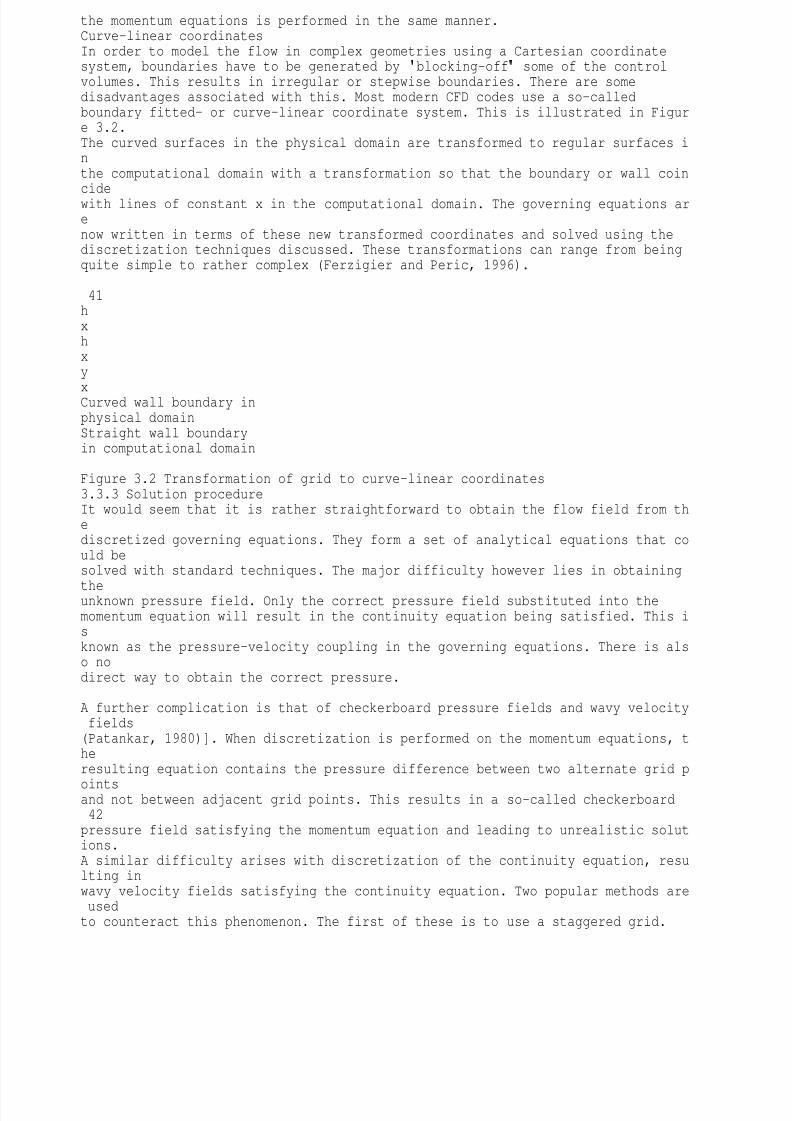
8/10/2019 Erasmus Mass 2004.PDF
http://slidepdf.com/reader/full/erasmus-mass-2004pdf 52/257
the momentum equations is performed in the same manner.Curve-linear coordinatesIn order to model the flow in complex geometries using a Cartesian coordinatesystem, boundaries have to be generated by blocking-off some of the controlvolumes. This results in irregular or stepwise boundaries. There are somedisadvantages associated with this. Most modern CFD codes use a so-calledboundary fitted- or curve-linear coordinate system. This is illustrated in Figure 3.2.The curved surfaces in the physical domain are transformed to regular surfaces inthe computational domain with a transformation so that the boundary or wall coincidewith lines of constant x in the computational domain. The governing equations arenow written in terms of these new transformed coordinates and solved using thediscretization techniques discussed. These transformations can range from beingquite simple to rather complex (Ferzigier and Peric, 1996).
41hxhxy
xCurved wall boundary inphysical domainStraight wall boundaryin computational domain
Figure 3.2 Transformation of grid to curve-linear coordinates3.3.3 Solution procedureIt would seem that it is rather straightforward to obtain the flow field from thediscretized governing equations. They form a set of analytical equations that could besolved with standard techniques. The major difficulty however lies in obtaining
theunknown pressure field. Only the correct pressure field substituted into themomentum equation will result in the continuity equation being satisfied. This isknown as the pressure-velocity coupling in the governing equations. There is also nodirect way to obtain the correct pressure.
A further complication is that of checkerboard pressure fields and wavy velocity fields(Patankar, 1980)]. When discretization is performed on the momentum equations, theresulting equation contains the pressure difference between two alternate grid p
ointsand not between adjacent grid points. This results in a so-called checkerboard42pressure field satisfying the momentum equation and leading to unrealistic solutions.A similar difficulty arises with discretization of the continuity equation, resulting inwavy velocity fields satisfying the continuity equation. Two popular methods are usedto counteract this phenomenon. The first of these is to use a staggered grid.

8/10/2019 Erasmus Mass 2004.PDF
http://slidepdf.com/reader/full/erasmus-mass-2004pdf 53/257
According to this method all the variables except velocity are computed at the centralgrid points (point P in Figure 3.2). The components of velocity are calculated at thepoints that lie on the face of a control volume. For the control volume shown in Figure3.2 these points would lie halfway between point P and all the other points insurrounding control volumes, i.e. on the six faces of the control volume. Thediscretized continuity equation would then contain differences between velocitycomponents at adjacent grid points. Similarly the discretized momentum equations would contain the pressure difference between adjacent grid points. There are someproblems associated with this method applied to non-orthogonal grids (Rhie andChow, 1983). Rhie and Chow (Rhie and Chow, 1983) proposed a method where asingle grid is used. The momentum equations are used to interpolate grid pointvelocities onto control volume faces in such a way as to avoid the use of pressuredifferences over alternating grid points.
An extra equation is however still needed to determine the unknown pressure field.This equation is known as the pressure correction equation.The pressure correction equation
This equation is derived by assuming that the correct pressure field is obtained byadding a pressure correction (p ) to the guessed pressure (p*):p p p *= + (3.49)This also gives rise to corresponding velocity corrections:
x x xU U U*= + y y yU U U*= + z z zU U U*= + (3.50)Discretization equations are obtained for the guessed velocity field (U*) usingtheguessed pressure field (p*). A discretization equation for the velocity correction field(U ) is also obtained (in terms of U and p ). These equations (one for eachcomponent of velocity) are then used for the velocity corrections U in Equation 3.50.
The pressure correction equation is now obtained by discretizing the continuityequation and substituting the velocity components with the corresponding velocitycorrection formula. A complete description of this method is beyond the scope of thistext and is given by Patankar (Patankar, 1980) and also by Rhie and Chow (Rhie andChow, 1983).43Solution algorithmThe solution algorithm that forms the basis for most commercial codes is the well-known SIMPLE algorithm (Patankar, 1980). The acronym SIMPLE stands for Semi-
Implicit Method for Pressure Linked Equations. The sequence of operations is:1. Guess the pressure field p* and the velocity field U*.2. Solve the momentum equations to obtain new values for U*.3. Solve the pressure correction equation to obtain p .4. Correct the pressure field by adding p to p*.5. Calculate U from the velocity correction formulas.6. Solve the discretization equations for the other variables (f
s) if they influencethe flow field.7. Treat the corrected pressure as the new guessed pressure and repeat the

8/10/2019 Erasmus Mass 2004.PDF
http://slidepdf.com/reader/full/erasmus-mass-2004pdf 54/257
procedure until a converged solution is obtained.There are a number of algorithms based on the original SIMPLE algorithm. The maindifference is the way in which the pressure correction equation is derived. Thewords
semi-implicit
refer to the omission of the influence of pressure correction on velocity.In the derivation of the pressure correction dicretization equation, the velocitycorrection terms are omitted. The converged solution obtained from using theSIMPLE algorithm does not contain errors resulting from this omission. Convergencedifficulties could however result from this. In algorithms like the SIMPLEC (Van Doormal and Raithby, 1984) the velocity correction equations are modified. Thisalsocauses a modification in the pressure correction equation and ultimately results in amore consistent correction field. This results in an overall faster convergencerate.3.4 CFD code used in this studyCFX-4.4 from AEA technology (Technology, 1999) was used in this study. Like most CFD codes, it is divided into three functional units: Pre-processor, Solver and
Post-processor. The pre-processor is used to construct the physical domain, specifyboundary surfaces and to create a grid. The solver transforms the grid from thephysical domain to the computational domain and solves the discretised equations.The post-processor is used for flow visualization. The main features of each oftheseunits will be briefly discussed next. For a complete discussion the CFX-4.4 user manual should be consulted (Technology, 1999).3.4.1 Pre-processorThe pre-processor is called CFX-4.4 Build. It contains a lot of the functionalities of a
conventional computer aided design package (CAD). The boundaries of the physical 44domain can therefore be created with this unit or alternatively imported from otherCAD design software. The major steps that have to be followed are:1. Create (or subdivide imported) geometry with a number of sub regions orblocks. Each of these blocks has to be a hexadron (contain six faces, eightvertices).2. Label boundaries according to type of condition imposed (inflow, outflow,pressure, periodic, wall etc.)3. Create structured surface mesh on all 2 dimensional surfaces.4. Generate hexahedral volume elements using 2D surface mesh.
The output of this unit contains all the geometric data of the multiblock grid (or body-fitted grid) in physical space and the location and type of boundaries imposed.3.4.2 SolverIn the solver part of the software the grid is transformed from the physical domain tothe computational domain. The governing equations are then discretised and solved.The major steps are:1. Transformation of the grid to the computational domain.

8/10/2019 Erasmus Mass 2004.PDF
http://slidepdf.com/reader/full/erasmus-mass-2004pdf 55/257
2. Discretization of governing equations3. Solving the discretised equationsThese steps will be discussed in turn next. Some comments regarding closuremodels will also be made.Transformation of grid to computational spaceThe grid in physical space is transformed to a grid in computational space. Forsimple rectangular geometries, the grid may be specified in this unit without importingit from the pre-processor. For a body fitted grid each block in the physical domainare transformed to a rectangular grid in the computational domain. This means thatthe coordinates are transformed (as discussed in curve linear coordinates) so thatthe boundaries in the physical domain coincide with one of the coordinate directionsin the computational domain. This results in a topological rectangular grid foreachblock in the computational domain. The different blocks with their rectangular grids inthe computational domain are then glued together to form the computational grid.Discretization of governing equationsThe next step is to discretise the governing equations. The governing equations
aretransformed to the computational domain coordinate system and discretised. A non-staggered grid is employed in the discretization. The velocity-pressure coupling in the45governing equations is treated according to the Rhie-Chow method (Rhie and Chow, 1983), as discussed in the section on the pressure correction equation. A number ofdifferent pressure-velocity coupling solution algorithms are available in the programwith the default being the SIMPLEC algorithm (Van Doormal and Raithby, 1984).
Solving the discretised equationsThe linearized (discretised) equations are not solved simultaneously, but rather by aniterative procedure. There are two steps employed in the method used by CFX-4.4. In the inner iteration the spatial coupling for a single variable is solved while in the
outer iteration
the coupling between variables is solved. In the
inner iteration thevalue for each variable is updated while regarding all the other variables as beingconstant. The non-linearity of the governing equations is simulated by updatingthe
coefficients in the discrete equations with the most recent calculated value for avariable before the
outer iteration
is performed. The pressure corrections are performed according to the velocity-pressure method and algorithm describedpreviously. A number of different convergence criteria may be specified for the
outeriteration or for global convergence. These range from specifying a global masssource residual to specifying residuals for specific variables There are also anumber

8/10/2019 Erasmus Mass 2004.PDF
http://slidepdf.com/reader/full/erasmus-mass-2004pdf 56/257
of ways in which damping may be employed. Full details are provided with thesoftware (Technology, 1999).
Closure models In this study turbulence modelling, and more specifically low Reynolds numberformulations of the eddy-viscosity two-equation models, was of high importance.CFX-4.4 contains the low Reynolds number BSL eddy-viscosity model of Menter,which is discussed in more detail in the paragraphs dealing with turbulencemodelling. In this regard CFX-4.4 was thought to be superior compared to otheravailable CFD codes.3.4.3 Post-processorThe post processor is known as CFX-Analyse. A variety of plots may be generatedwith this software. These include vector plots, fringe plots and particle tracklines. Itmay also be used for animated flow visualization.3.5 Implementation of CFD in this studyThe ideal model for mass transfer inside structured packing would be to divide thecolumn into a large number of small control volumes. The discretised equations of46fluid motion, mass- and heat transfer may then be simultaneously solved for allthecontrol volumes, subject to some specified boundary conditions. At present sucha
model is not possible. Only elementary physical models are available to modelcounter current stratified two phase flow. Even if more accurate and robust modelswere available, then the sheer number of control volumes needed to capture all thedetails of the multi phase flow field in a bed of structured packing would makesuch amodel impossible. With the elementary physical models currently available it ispossible to model the vapour/liquid interface in flow fields where there is no largeshear force at the interface between the two phases. Extremely fine grids are thennecessary in regions where the interface is expected to be. Since it is usually
notknown where the interface between the phases will be, a fine grid has to be createdover the entire physical domain.
At present it is therefore possible to model only the vapour phase flow insidestructured packing with some degree of accuracy. The vapour phase mass transferrate may be modelled by assuming that the boundary of the physical domaincoincides with the interface between the vapour and liquid phases. If it is furtherassumed that equilibrium is maintained at the interface between the two phases,thenthe equilibrium concentration of the species transferring into the physical doma
in maybe specified as a wall boundary. The vapour phase mass transfer coefficient maybecalculated by performing a mass balance for this species between the inlet and outletboundaries. This approach was tested in this study by modelling the mass transferrate for a species evaporating in a short counter current wetted-wall column. Thevalues for the mass transfer coefficient obtained in this manner compared favour

8/10/2019 Erasmus Mass 2004.PDF
http://slidepdf.com/reader/full/erasmus-mass-2004pdf 57/257
ablywith experimental results. Full details are provided in Chapter 5.
As mentioned before, despite recent advances in computing power, it is at presentnot possible to model a complete bed of structured packing. This is even more truewhen a low Reynolds number formulation of a two-equation eddy-viscosity typeturbulence model (like the k-e or k-w turbulence models) is used. The grid has to berefined to such an extent near the wall that extremely fine grids are necessarytoobtain convergence compared to when using the same model with a wall function.The use of the low Reynolds number formulation of these turbulence models wasdeemed necessary in order to model mass transfer from a wall boundary.
The bed may, however, be broken down into smaller re-occurring sub-domains. ACFD model is set up for each of these sub-domains. The bed is then reconstructed 47by adding the contribution from each sub-domain. The contributions are calculatedfrom the number of times that such a sub-domain re-occurs in the bed. A number of
previous investigators have followed this approach (Ciofalo et al., 1996, Hodson,1997, Hodson et al., 1997, Larachi et al., 2003, Petre et al., 2003). From a masstransfer point of view, the most important sub-domain or micro element, is thejunction between two cross-corrugated channels. There are three other sub-domainsor micro elements also occurring in a bed of packing. These may be visualized by tracing the path that the vapour follows when flowing through a bed of structuredpacking and are explained by referring to Figure 3.3. Micro element 1 is found at the
base of the bed where the vapour phase enters the bed of packing. Micro element2is the junction between two cross-corrugated channels. A number of these elementsare found before a channel either ends up at the column wall, or reach the horizontalplane where two packing segments meet. At the column wall micro element 3 isfound. The vapour is deflected from the wall and switch from the channel of theparent sheet to a channel starting at the wall on the sheet facing the parent sheet. Atthe horizontal plane where two packing segments meet, the vapour phase undergo a sharp change in direction (total direction change not shown in Figure 3.3. The m
icroelement that re-occurs the most is the junction between corrugated passages (microelement 2). It has been shown that it causes between 65% and 72% of the dry bedpressure drop over the packing (Petre et al., 2003, Larachi et al., 2003). In this studythe focus has been on the CFD modelling of micro element 2. The bulk of thepacking may be reconstructed by arranging a number of these micro elements inseries. The outlets of one element are used as the inlets to the next element and the

8/10/2019 Erasmus Mass 2004.PDF
http://slidepdf.com/reader/full/erasmus-mass-2004pdf 58/257
process is repeated for the whole length of a corrugated channel.
The approach outlined above for modelling the vapour phase mass transfer rateinside structured packing was followed in obtaining the CFD results shown in Chapter5. Since the aim of this chapter is to introduce the general modelling approach, moredetails on the physical domain, computational grid and boundary conditions may befound in Chapter 5.481234
Figure 3.3 Breakdown of structured packing into re-occurring micro elements.493.6 NomenclatureA Area [m2]a Influence coefficients [-]g Gravitational acceleration [m/s2]k Turbulent kinetic energy [m2/s2]
P Peclet number [-]p Pressure [Pa]Pk Production of turbulent kinetic energy [kg/(m3s2]S Source term [-]u Component of velocity [m/s]U Velocity vector [m/s]U Velocity fluctuation vector [m/s]U Time averaged velocity vector [m/s]V Volume [m3]x,y,z Cartesian coordinates [m]GreekDel operator
m Molecular (dynamic) viscosity [kg/(m.s)]
mt Turbulent (eddy) viscosity [kg/(m.s)]h,x Curve linear coordinates [m]G Diffusion coefficient (diffusivity) [kg/(m.s)]Gt Turbulent (eddy) diffusivity [kg/(m.s)]d distance from point to control volume face [m]e Turbulent kinetic energy dissipation rate [m2/s3]f Variable [-]r Density [kg/m3]st Turbulent Prandtl/Schmidt number [-]t Stress [Pa]w Pseudo vorticity [1/s]Subscriptsb Refers to control face beneath point P
B Refers to grid point beneathe Refers to control face to the east of point P50E Refers to grid point to the eastn Refers to control face to the north of point PN Refers to grid point to the northP Centre point of control volumes Refers to control face to the south of point PS Refers to grid point to the southt Refers to control face above point P
8/10/2019 Erasmus Mass 2004.PDF
http://slidepdf.com/reader/full/erasmus-mass-2004pdf 59/257
T Refers to grid point abovew Refers to control face to the west of point PW Refers to grid point to the westSuperscript0 Values at time tf Refers to property of general variable
514 HYDRODYNAMICS4.1 IntroductionFor both equilibrium and rate-based simulations it is important to know the hydrauliccapacity of packing, since it determines the diameter of the column. With anequilibrium simulation the column diameter is determined after determining the flowrates and compositions in the column. With a rate-based simulation, the diameter ofthe column is an input parameter into the model. The modelling of the hydrauliccapacity is therefore important if an accurate rate-based simulation is to beperformed. The lack in reliable hydraulic models has lead to limited use of rate-basedsimulations. A few new hydrodynamic models have recently been developed (Olujicet al., 1999, Olujic, 1997, Brunazzi and Pagliante, 1997) and there have also be
enrefinements to existing models (Fair et al., 2000, Billet, 1995). In this chapter thesehydrodynamic models are discussed and compared with measured experimentaldata. The recent improvements in the hydraulic capacity of structured packing arealso investigated (Billingham and Lockett, 1999).4.2 Literature survey4.2.1 Basic conceptsBefore discussing the methods and correlations used to predict the hydrauliccapacity of structured packing, it is first necessary to introduce a few basic concepts.These concepts are discussed with relation to Figure 4.1 and Figure 4.2. Figure
4.1represents the pressure drop over a packed bed and Figure 4.2 shows the hold-up. On both graphs these quantities are plotted against the superficial vapour velocity.Figure 4.1 shows that the pressure drop curve at a specific liquid load is parallel tothe pressure drop curve for the dry packing up to a certain point. Beyond this pointthe pressure drop increases rapidly with an increase in the superficial vapour velocity(the slope of the curve increases). In Figure 4.2 this point coincides with theliquid
hold-up starting to be influenced by the vapour velocity. Up to this point the hold-up isindependent of the superficial vapour velocity and only dependent on the liquidloadand liquid properties. This point shifts to lower superficial vapour velocitieswith anincrease in liquid load. In Figures 4.1 and 4.2 these points are represented with lineA-A. Beyond this point the slope of the hold-up curve increases rapidly up to the point
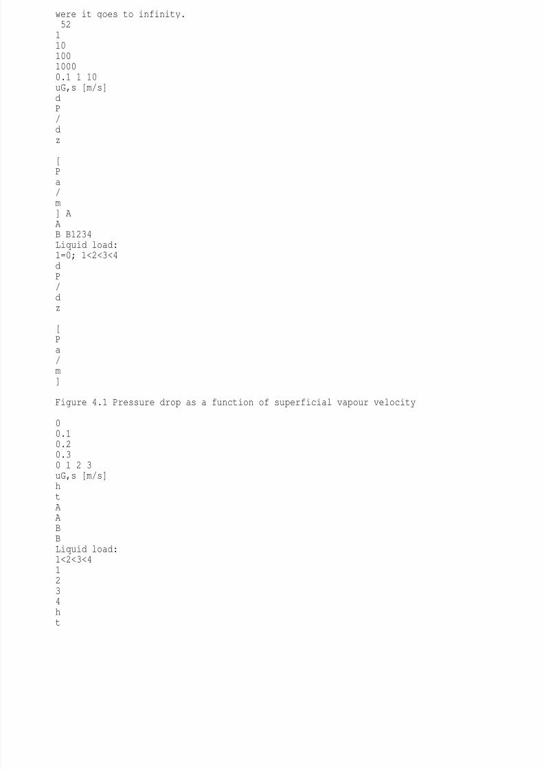
8/10/2019 Erasmus Mass 2004.PDF
http://slidepdf.com/reader/full/erasmus-mass-2004pdf 60/257
were it goes to infinity.5211010010000.1 1 10uG,s [m/s]dP/dz [Pa/m] AAB B1234Liquid load:1=0; 1<2<3<4
dP/dz [Pa/m]
Figure 4.1 Pressure drop as a function of superficial vapour velocity
00.10.20.30 1 2 3uG,s [m/s]htAAB
BLiquid load:1<2<3<41234ht
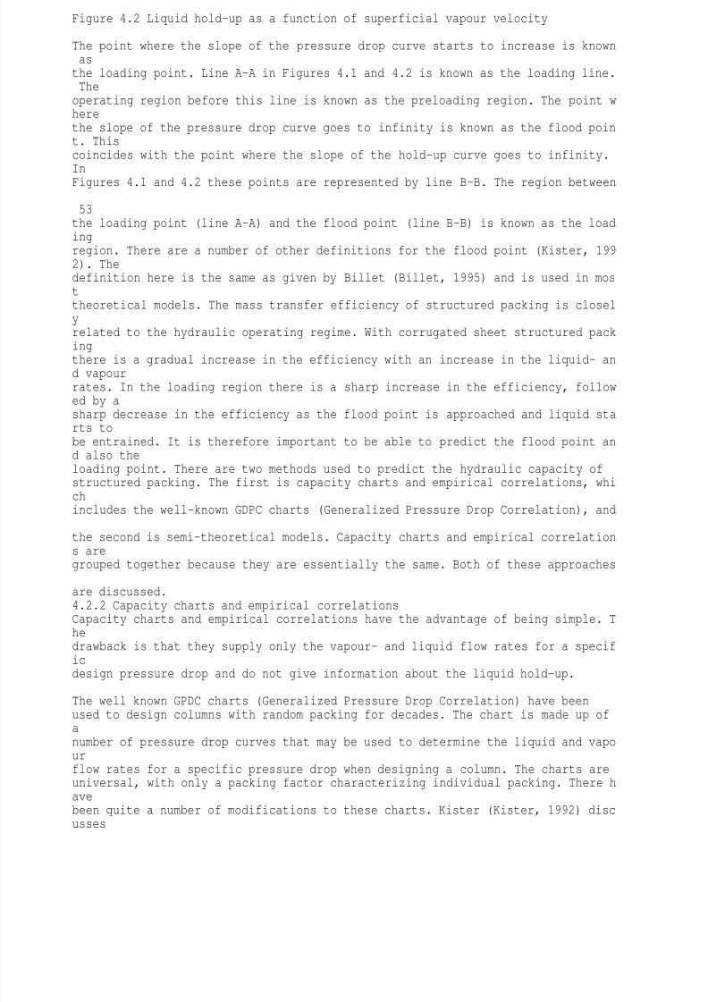
8/10/2019 Erasmus Mass 2004.PDF
http://slidepdf.com/reader/full/erasmus-mass-2004pdf 61/257
Figure 4.2 Liquid hold-up as a function of superficial vapour velocity
The point where the slope of the pressure drop curve starts to increase is known asthe loading point. Line A-A in Figures 4.1 and 4.2 is known as the loading line. Theoperating region before this line is known as the preloading region. The point wherethe slope of the pressure drop curve goes to infinity is known as the flood point. Thiscoincides with the point where the slope of the hold-up curve goes to infinity.InFigures 4.1 and 4.2 these points are represented by line B-B. The region between 53the loading point (line A-A) and the flood point (line B-B) is known as the loadingregion. There are a number of other definitions for the flood point (Kister, 1992). Thedefinition here is the same as given by Billet (Billet, 1995) and is used in mosttheoretical models. The mass transfer efficiency of structured packing is closelyrelated to the hydraulic operating regime. With corrugated sheet structured pack
ingthere is a gradual increase in the efficiency with an increase in the liquid- and vapourrates. In the loading region there is a sharp increase in the efficiency, followed by asharp decrease in the efficiency as the flood point is approached and liquid starts tobe entrained. It is therefore important to be able to predict the flood point and also theloading point. There are two methods used to predict the hydraulic capacity ofstructured packing. The first is capacity charts and empirical correlations, whichincludes the well-known GDPC charts (Generalized Pressure Drop Correlation), and
the second is semi-theoretical models. Capacity charts and empirical correlations aregrouped together because they are essentially the same. Both of these approaches are discussed.4.2.2 Capacity charts and empirical correlationsCapacity charts and empirical correlations have the advantage of being simple. Thedrawback is that they supply only the vapour- and liquid flow rates for a specificdesign pressure drop and do not give information about the liquid hold-up.
The well known GPDC charts (Generalized Pressure Drop Correlation) have beenused to design columns with random packing for decades. The chart is made up ofanumber of pressure drop curves that may be used to determine the liquid and vapourflow rates for a specific pressure drop when designing a column. The charts areuniversal, with only a packing factor characterizing individual packing. There havebeen quite a number of modifications to these charts. Kister (Kister, 1992) discusses

8/10/2019 Erasmus Mass 2004.PDF
http://slidepdf.com/reader/full/erasmus-mass-2004pdf 62/257
these in detail. There are results from a few studies that are presented in theform ofsimilar capacity charts.
The first published comprehensive study was by McNulty and Hsieh (McNulty andHsieh, 1982). They measured and characterized the hydraulic performance andefficiency of the Flexipac range of structured packing from Koch in a 3 foot diametercolumn. Air and water was used at ambient conditions to perform the experimental work. The GPDC method for predicting pressure drop and capacity was found to beinadequate for Flexipac structured packing. Over the liquid loads investigated,thepacking factor had to be varied by a factor of two for the GPDC curves to fit the54experimental data. The so-called `CGCL' method is proposed to correlate theflooding point for the different packing investigated. The `CGCL' model uses thecapacity factors CG and CL to correlate the velocity and density dependence ofpressure drop and flooding. The correlation suggests a linear relationship for theflooding points in terms of CG½ and CL½. Experimental data confirmed this trend. The influence of liquid viscosity and surface tension was not investigated experimen
tally.The `CGCL' model was modified to include viscosity effects by incorporating thesame viscosity dependence as has been used in the GPDC model. Surface tensioneffects were neglected because the surface tension varies within a narrow band formost applications. Efficiency tests were also performed by doing heat transferexperiments. These tests showed that the efficiency increased with an increase inliquid flow rate and this was attributed to better spreading and wetting behaviour ofthe packing at higher liquid flow rates. Efficiency was found to be `reasonablyindependent' of vapour flow rate up to a certain point. An increase in vapour flow rate
beyond this point caused a sharp decrease in efficiency. This point is called themaximum design vapour velocity and was found to be at approximately 80% offlooding for a given liquid flow rate. The capacity factor for the vapour- and liquidphases are given by:r=r - rGG G,sL GC u (4.1)LL L,sL G
C u r= r - r (4.2)The correlation to determine the flood point (or any percentage there of) is:
+ = m1 12G 2L0.03C cmCf (4.3)m is the viscosity of the fluid relative to that of water at 70oF (1cP) and f is

8/10/2019 Erasmus Mass 2004.PDF
http://slidepdf.com/reader/full/erasmus-mass-2004pdf 63/257
the fractionof flooding. For design purposes, a value of f=0.8 is recommended. Values for mandc are given for the different types of Flexipac (McNulty and Hsieh, 1982).
Spiegel and Meier (Spiegel and Meier, 1987) characterized the Mellapak range ofstructured packing using chloro-/ethylbenzene and trans-/cis-decalin test mixtures attotal reflux in a column with an internal diameter of 1m. The capacity results areplotted on both a Souders and a Wallis diagram. The results are correlated withanequation of the form:551 12 2G LC mC c+ = (4.4)where m and c are adjustable constants. The exact values of these constants arenotgiven but the correlation are reported to predict the capacity with an accuracyof 6%.
The attempts by McNulty and Hsieh (McNulty and Hsieh, 1982) to apply the GDPCcharts to structured packing were one of several attempts that were only partially
successful. Kister and Gill (Kister and Gill, 1992) identified the limitations of theGDPC charts and proposed the following modifications. The abscissa is the flowparameter and is defined as:0.5GLLXG
r= r (4.5)The ordinate is the capacity parameter:0.5 0.05S PY C F= n (4.6)
FP is an empirical factor that characterizes the packing shape and size. CS is thesuperficial vapour velocity corrected for density:GS G,sL GC u r= r - r (4.7)A list of packing factors for well known commercial packing is provided (KisterandGill, 1992). The proposed chart is called the GPDC (SP) interpolation chart. The available experimental data for each type and size of packing is also plotted on thechart. This makes it possible to interpolate between experimental values in oper
atingregions where data are available. Kister (Kister, 1992) provides charts for most of theavailable commercial structured packing. They also found that the pressure dropatwhich flooding occurs is accurately correlated by:0.7flood PP 0.115FD = (4.8)with dimensions [in H2O/ft].Robbins (Robbins, 1991) proposed a correlation to predict pressure drop andflooding for random and structured packing. At low liquid loadings, the pressure

8/10/2019 Erasmus Mass 2004.PDF
http://slidepdf.com/reader/full/erasmus-mass-2004pdf 64/257
dropdepends only on the vapour flow rate and the geometry of the packing. The packingfactors are calculated from dry bed pressure drop data. The correlation is plotted ona chart with the pressure drop as a function of a vapour capacity factor. Pressuredrop curves are provided on the chart for different liquid-to-vapour capacity factorratios. It is generally not recommended for operation at elevated pressures (Kister,1992).564.2.3 Semi-theoretical modelsThere are quite a few semi-theoretical models published for random- and structuredpacking. These models are in the form of equations and correlations that can beimplemented into numerical algorithms. They can be divided into two categories:channel models and porous bed or particle models. In the channel type models the packed bed is modelled as a series of inclined wetted-wall channels. The liquidandvapour is split up, uniformly or non-uniformly, between the different channels.Pressure drop is due to skin friction, form drag and abrupt changes in the flow
path.Hold-up in the bed causes the liquid films to become thicker and decrease the totalarea available for the vapour flow. Examples of channel models are those due toBravo et al. (Bravo et al., 1985, Bravo et al., 1986), Rocha et al. (Rocha et al., 1993),Billet et al. (Billet, 1995), Brunazzi et al. (Brunazzi and Pagliante, 1997) and Olujic etal. (Olujic, 1997, Olujic et al., 1999). In the particle model the column is modelled asa packed bed using the classic Ergun equation. Pressure drop is due to form drag associated with the particles. The liquid hold-up in the bed reduces the void fr
actionof the bed and increases the dimension of the particles. Because of the well orderednature of structure packing and its close resemblance to a series of inclined wetted-walls, there are only a few porous bed (or particle) type models developed forstructured packing. A well known particle model is that of Stichlmair et al. (Stichlmairet al., 1989). A more detailed discussion of some of the models will follow.Channel modelsThe SRP model was developed at the University of Texas over several years (Bravo et al., 1985, Bravo et al., 1986, Fair et al., 2000, Rocha et al., 1993, Rocha a
ndBravo, 1996). The first model (Bravo et al., 1986) was fitted on air-water pressuredrop data for two types of packing, the Flexipac range of packing (McNulty andHsieh, 1982) and the Gempak range of packing. The dry pressure drop over the bed is correlated with a Darcy type equation:2G,eGhGd
8/10/2019 Erasmus Mass 2004.PDF
http://slidepdf.com/reader/full/erasmus-mass-2004pdf 65/257
udP fdz d
= r (4.9)The friction factor is given by:21G,eCf CRe= + (4.10)where C1 and C2 are packing specific constants. The pressure drop over an irrigatedbed is correlated with an expression similar to that developed for random packing:575tddP dP 1dz dz 1 h
=
-
8/10/2019 Erasmus Mass 2004.PDF
http://slidepdf.com/reader/full/erasmus-mass-2004pdf 66/257
(4.11)The liquid hold-up is correlated with the Froude number:0.5t 3 Lh C Fr= (4.12)In total three packing specific constants are needed. These constants are publishedfor the Flexipac and Gempak range of packing (Bravo et al., 1986). The model doesnot apply to conditions where the loading causes significant liquid hold-up.
The model was extended by Rocha et al. (Rocha et al., 1993) in order to predictpressure drop and hold-up in the loading region. The correlations for the dry pressuredrop and friction factor are the same as previously (Equation 4.9 and 4.10). The irrigated pressure drop is calculated with an expression similar to Equation 4.11, withthe addition of an extra constant:52 tddP dP 1dz dz 1 K h
=
-

8/10/2019 Erasmus Mass 2004.PDF
http://slidepdf.com/reader/full/erasmus-mass-2004pdf 67/257
(4.13)where2K 0.614 71.35S= + (4.14)with S the side dimension of a corrugated passage.In order to calculate the liquid hold-up an effective gravity is used. It is derived byperforming a force balance on a fluid element. The final form of the equation is:( )L GeffL flooddP / dzg g 1dP / dz
r - r
= - r

8/10/2019 Erasmus Mass 2004.PDF
http://slidepdf.com/reader/full/erasmus-mass-2004pdf 68/257
(4.15)The pressure drop at flooding needs to be prescribed and in the model it is assumedto be constant at 1025 Pa/m. The film thickness and wetted area is used to calculatethe liquid hold-up. The film thickness is calculated according to the classic equationfor a laminar falling film, utilizing the effective gravity. A The final form of the equationfor liquid hold-up is:( )1233 L L,sttL eff3 uFh 4S sin g
m = r q e (4.16)The term Ft is a correction factor to account for under wetting of the packing and is
based on the Shi and Mersmann (Shi and Mersmann, 1985) correlation for effective interfacial area in random packing:58( )( )( )0.15 0.359L Lt0.30.2 0.6L29.12 We Fr SFRe 1 0.93cos sin=
e - g q (4.17)Expressions were developed for the constants in the model based on thecharacteristic dimensions of seven types of common commercial structured packing.Information needed in the model is the pressure drop at which flooding occurs andthe dry pressure drop over the packing.
More recently (Fair et al., 2000) the model was changed by implementing the loadingpoint correlation by Verschoof et al (Verschoof et al., 1999) and renamed the SRP
model. The pressure drop in the loading region is calculated with:loadpreloaddP dP Fdz dz
= (4.18)The pressure enhancement factor for the loading region is given by:q

8/10/2019 Erasmus Mass 2004.PDF
http://slidepdf.com/reader/full/erasmus-mass-2004pdf 69/257
= e 0.132 / sin 2L,sGload 2G,lp hGuFF 3.8F gd (4.19)The loading point F-factor is calculated with:( ) ( )- r
= e r - r q r 0.50.251.15L,s2 LG,lp hG L GG,s GuF 0.053 gd sinu (4.20)Billet (Billet, 1995) developed a model for both random and structured packing.Mostof the experimental data on which the model was fitted were for random packing.There are quite a number of packing specific constants in the model. This makes
themodel less applicable to structured packing, as only a few types of structured packingwere characterized in the study. A broad range of random packing was used and allthe necessary packing specific constants in the model for these packing arepublished (Billet, 1995). Some structured packing data are also included. Althoughmost of the quantities are calculated with correlations, a fundamental approachwasfollowed in deriving the specific form of these correlations. An equation describing thecounter current two-phase flow was developed and then used as the basis for
developing the different correlations. The dry pressure drop is calculated with: = x r e2p G,sd G s3da udP fdz 2 (4.21)where59
x = +
d p 0.08G,s G,s64 1.8CRe Re (4.22)and= +s p c1 41f a d (4.23)The irrigated pressure drop is calculated from:3

8/10/2019 Erasmus Mass 2004.PDF
http://slidepdf.com/reader/full/erasmus-mass-2004pdf 70/257
wd tddP dPdz dz h
x e = x e - (4.24)where( ) e -
x = + e 1.5tw p0.08G,s G,sh64 1.8C WRe Re (4.25)and
=
8/10/2019 Erasmus Mass 2004.PDF
http://slidepdf.com/reader/full/erasmus-mass-2004pdf 71/257
0.3L,s tt,lpRe hW exp200 h (4.26)In order to determine the pressure drop, values for the hold-up are needed. Thereare two different types of hold-up calculated with the model. The first hold-upis usedto calculate the pressure drop over the packing. Complete wetting is assumed incalculating this hold-up. The hold-up at the loading point is calculated from:- r
= m 111 2 33L,s pL,s L3t,lpp Lu auh 12a g (4.27)The hold-up at the flood point is correlated from experimental data as:ms/kg4101L
05.0WWLLfp,t 3741.0h -·>m
mrrme= (4.28)
Subscript W refers to the properties of water. The hold-up above the loading point iscalculated from:( ) ( ) ( ) ( )G,s G,slp13G,st t,lp t,fp t,lpu uG,s fpuh h h hu>
= + -
(4.29)In the second approach non-uniform wetting is assumed. The hold-up at the loadingpoint is determined from:60( ) ( )£ m = = r
G,s G,s lp1 2

8/10/2019 Erasmus Mass 2004.PDF
http://slidepdf.com/reader/full/erasmus-mass-2004pdf 72/257
2 3 3L L,sht t,lpu u L pa u ah h 12g a (4.30)The ratio of the hydraulic area to the wetted area (ah/ap) is calculated with:<
= L0.15 0.1h h L,s L,sp Re 5a C Re Fra (4.31)³
= L0.25 0.1h h L,s L,sp Re 5a 0.85C Re Fra (4.32)The liquid hold-up at the flood point was found to be approximately 2.2 times higher
than the hold-up below the loading point:t,fp t,lph 2.2h@ (4.33)The hold-up between the loading- and flood points is calculated with Equation 4.29.In order to calculate hold-up and pressure drop, the superficial vapour velocities atthe load- and flood points have to be determined. The superficial vapour velocity atthe loading point is calculated from:( ) ( ) r= e -x rt,lp LG,s t,lplplp p Ghgu ha (4.34)
where the resistance factor is defined as:lplp 2n0.42 LlpGgCx =
m
y m

8/10/2019 Erasmus Mass 2004.PDF
http://slidepdf.com/reader/full/erasmus-mass-2004pdf 73/257
(4.35)The superficial vapour velocity at the flood point is given by:( ) ( )e - r= x re3 2t,fp t,fp LG,s 1 2fpfp p Gh h2gu a (4.36)The resistance factor differs slightly from the definition in Equation 4.35:fpfp 2n0.22 LfpGgCx =
m
y m

8/10/2019 Erasmus Mass 2004.PDF
http://slidepdf.com/reader/full/erasmus-mass-2004pdf 74/257
(4.37)In order to use the model, four packing specific constants are needed: Cp, Ch, Clp andCfp. As mentioned before, a large number of these constants are available for61random packing (Billet, 1995). The number of constants available for structuredpacking limits the use of the model.
In the pressure drop model by Brunazzi et al. (Brunazzi and Pagliante, 1997), thetotal pressure drop is calculated as the sum of friction, gravitation and accelerationterms:TOT F G AdP dP dP dPdz dz dz dz
= + + (4.38)The friction term is split up into contributions from losses at the channel walls and atthe vapour-liquid interface (distributed losses), and losses from changes in the flow
direction (concentrated losses):F F,d F,cdP dP dPdz dz dz
= + (4.39)For the dry pressure drop the different terms are:Acceleration term:G,eG G,sAdudP u
dz dz = r (4.40)Gravitational term:GGdP gdz
= -r (4.41)Distributed frictional term:
( )wG GGF,ddP 1 Sdz A sin
= t q (4.42)AG is the channel area and SG is the channel perimeter (defined using the equivalentdiameter). The shear stress at the channel wall is calculated from:2wG G G G,e1 f u
8/10/2019 Erasmus Mass 2004.PDF
http://slidepdf.com/reader/full/erasmus-mass-2004pdf 75/257
2t = r (4.43)The friction factor is calculated with:2G 1GBf BRe= + (4.44)B1 and B2 are packing specific constants. The concentrated frictional term iscalculated from:2eq G G,eG chGF,cL udP 4f Ndz d 2r =
(4.45)62Nc is the number of bends per unit height of packing and Leq is the equivalent lengthof a channel. The values of these constants are dependent on the height of a packingelement and the corrugation angle and are given by Brunazzi et al. (Brunazzi and
Pagliante, 1997). In order to calculate the irrigated pressure drop, the wettedareahas to be known to calculate frictional losses at the vapour-liquid and vapour-solidinterfaces respectively. From the equation for the film thickness of a laminar fallingfilm the following equation is derived:0.51.5e hG Ltp L L,sa d sin gha 4 3 u
q r =
e m (4.46)For the irrigated pressure drop the gravitational term is the same as for the drypressure drop. The distributed frictional term is given by:( )wG G i iGF,ddP 1 1S Sdz A sin
= t + t q (4.47)SG and Si are the dry and wet channel perimeters respectively and AG is the avai
lablearea for the vapour phase. In calculating these quantities allowance are made for theliquid hold-up (Brunazzi and Pagliante, 1997). The shear stress at the vapour-liquidinterface is calculated from:( )2i i G G,e L,e1 f u u2t = r + (4.48)The friction factor is calculated using an equation similar to that proposed for countercurrent annular two-phase flow:

8/10/2019 Erasmus Mass 2004.PDF
http://slidepdf.com/reader/full/erasmus-mass-2004pdf 76/257
5o0.1B0.3 0 Li G 3 4 LhG W,20 Cf f 1 B Bo B Wed
d - d m
= + +
m

8/10/2019 Erasmus Mass 2004.PDF
http://slidepdf.com/reader/full/erasmus-mass-2004pdf 77/257
(4.49)The concentrated frictional term is given by:2eq G G,em chGF,cL udP 4f Ndz d 2r =
(4.50)fm is a mean friction factor, weighed on the wetted area and calculated from the wall-and interfacial friction factors. The film thickness is calculated from:2 L,ei i LL L LchanLLchanudP4 gsin2 2 dz 32 dPgsin3 dz
t t + ± + r q- m m m

8/10/2019 Erasmus Mass 2004.PDF
http://slidepdf.com/reader/full/erasmus-mass-2004pdf 78/257
r q-
m
8/10/2019 Erasmus Mass 2004.PDF
http://slidepdf.com/reader/full/erasmus-mass-2004pdf 79/257
d = (4.51)where63Gchan F,ddP dP sin gsindz dz
= q - r q (4.52)The liquid hold-up is calculated from the correlation proposed by Suess et al. (Suessand Spiegel, 1992):( ) m = m
o0.25x0.83 Lt p L,sW,20 Ch C a 3600u (4.53)In total six characteristic constants are needed in the model. Constants are availablefor Sulzer Mellapak 250Y/X and BX packing made from metal or plastic (Brunazzi
and Pagliante, 1997).
In the Olujic et al. (Olujic et al., 1999) model the vapour flows in a zigzag patternthrough the different packing elements along the triangular channels formed by thecorrugated sheets. The pressure drop in the preloading region is calculated with theconventional Darcy type pressure drop equation. In calculating the loss coefficient,three contributions to pressure loss are identified. The first is the overall vapour/liquidinteraction, into which losses due to vapour/liquid friction is lumped. The seco
nd islosses due to vapour interaction between adjacent triangular channels and the thirdis pressure losses due to directional changes of the vapour and liquid phases:( )2G G,eGL GG DCpreloadudPdz 2r = z + z + z
(4.54)The overall vapour/liquid interaction coefficient is calculated with:
z = jx qpbGL GLhGhd sin (4.55)and the vapour/liquid friction factor from:( ) ( ) 2hG hGGLG,r G,r/ d / d5.02 14.52log log3.7 Re 3.7 Re

8/10/2019 Erasmus Mass 2004.PDF
http://slidepdf.com/reader/full/erasmus-mass-2004pdf 80/257
- d d x = - - +
8/10/2019 Erasmus Mass 2004.PDF
http://slidepdf.com/reader/full/erasmus-mass-2004pdf 81/257
(4.56)The vapour/vapour interaction coefficient is calculated with:( ) ( )z = - j q qpb3.14GGhGh1 0.722 cosd sin (4.57)Losses due to directional changes are given by:( )pbDC bulk wallpehhz = x + yx (4.58)The fraction of channels ending against a wall is:64
y = + p qp q q 0.52pe pe pe2c2 2cc2h h h2d arcsind tand tan tan (4.59)The loss coefficient at the interface between packing elements is given by:( )x = q 1.63bulk 1.76 cos (4.60)
and the loss coefficient of channels ending at a wall by:( ) ( )+ qx = + q0.4450.31 0.779L,s 0.44wall L,sG,e4092u 4715 cos 34.19u cosRe (4.61)The pressure drop in the loading region is calculated using the correlations proposedby Verschoof et al. (Verschoof et al., 1999) for predicting the loading point andloading effect. The same equations are used as discussed in the SRP model. Theliquid hold-up is calculated simply from the geometric area of the packing and the
liquid film thickness:t ph a= d (4.62)The liquid film thickness is calculated with the Nusselt formula for falling films,provision being made for the inclination angle of the packing:
md = r q 13L L,sL p3 uga sin (4.63)
There are no packing specific constants in the model. All the constants needed in themodel are calculated using the characteristic lengths B, S and h of corrugatedstructured packing.
There are a few more recent models that are also classified as channel models.These models are more fundamental in nature and have been developed to predictpressure drop and hold-up in the preloading region. Because of the fundamentalnature of these models, the model equations are quite complicated. These modelsare probably a start to a new generation of hydraulic models. Their complexity a

8/10/2019 Erasmus Mass 2004.PDF
http://slidepdf.com/reader/full/erasmus-mass-2004pdf 82/257
ndlimited range limits their use in hydraulic calculations at present.
Woerlee et al (Woerlee et al., 2001) developed a fundamental model for pressuredrop in packed columns. The packed bed is modelled as a series of inclined tubes.The liquid is modelled as a laminar film that totally wets the tube walls. The pressuredrop comprises of frictional losses at the vapour-liquid interface and losses due to thegeometry or form drag. The friction factor for a smooth liquid interface is calculated65with the Blasius equation. The pressure drop due to form drag and geometry iscombined with the interfacial losses using the Ergun equation for packed beds. Thefriction factors are then determined by fitting the Ergun relation on experimental data(dry packing). The proposed equation for the friction factor is extended to includewhat is termed as the `effective' packing inclination angle. This angle is calculatedfrom dry pressure drop data. A modification is also made to take column diameter
effects into account. The increase in pressure drop due to the presence of adisturbed liquid film (not smooth any more) is taken into account by defining avapour-liquid interaction coefficient. The pressure drop for a smooth (non-disturbed)film is then multiplied by this factor to calculate the overall total pressure drop. Thisinteraction coefficient is determined by fitting the model to experimental data. Themodel did not predict the pressure drop in structured packing accurately. This isthought to be due to liquid entrainment (Woerlee et al., 2001).
Iliuta and Larachi (Iliuta and Larachi, 2001) proposed a hydraulic model for str
ucturedpacking in the preloading region. The model is based on the hydrodynamic modellingof concurrent two phase flow in a randomly packed trickle bed reactor. In the modelthe irrigated pressure drop, liquid hold-up and fraction wetted area is simultaneouslycalculated. Inputs needed are the dry pressure drop for the specific packing and thepacking constants. The packing is assumed to be partially wetted. The partiallywetted packing is conceptually split up into wet channels and dry channels (or slits).The vapour flow rate is split up between the dry and wet channels. The dimension
s ofthese channels are related to the packing geometry. A few simplifying assumptionsregarding the flow are made. A smooth vapour-liquid interface is assumed. Thecontribution made to the effective surface area by liquid droplets is assumed to benegligible. The effective phase velocities in the channels or slits are identical to theeffective velocities in the packing geometry. The friction factors at the wall and at the
8/10/2019 Erasmus Mass 2004.PDF
http://slidepdf.com/reader/full/erasmus-mass-2004pdf 83/257
vapour-liquid interface are equal. There are no discontinuities in the velocityandshear profiles at the vapour-liquid interface and the pressure drop across theconceptual channels (slits) are equal to the pressure drop over the packed bed.Momentum balances are performed for the vapour phase in the dry and wet channels and for the liquid phase in the wet channels. An expression is developed for the liquidvelocity at the interface and the average liquid film velocity. After some simplification,the model consists of three non-linear coupled algebraic equations that are solvedwith an iterative technique. The results compare favourably with experimental resultsand with the model of Billet (Billet, 1995).
66Ranke et al. (Ranke et al., 2000) suggested a model to predict pressure drop and hold-up based on experimental work carried out on two types of structured packingmade from aluminium and with a specific surface area of 750m2/m3. An organic liquidwas used in the experiments and the vapour entering the column was saturated wit
hthe liquid. In developing the model it is assumed that the vapour follows the channelsprovided by the packing. The liquid phase stays on a single corrugated sheet and follows a path down the plane with the steepest inclination angle. The angle atwhichthe liquid flows down the sheet is influenced by the interfacial shear stress at thevapour-liquid interface. In calculating the dry pressure drop, the friction factor is splitup into contributions from interfacial friction, losses due to changes in direction
between packing elements and losses due to the outflow of vapour from a packedsection. A force balance for the liquid film is done and shear at the vapour-liquidinterface is taken into account. This yields an equation from which the velocity distribution and film thickness can be obtained (after integration). The dynamic liquidhold-up is determined from the geometric area of the packing and the average liquidfilm thickness. Complete wetting of the packing is assumed. The irrigated pressuredrop is calculated from the dry pressure drop multiplied by the ratio of the `available
cross sectional area' for vapour flow raised to the power 2.5. A radial distributionmodel was developed for the liquid phase. At each contact point a portion of the liquid flows to the adjacent sheet. Lateral liquid shift is also thought to be generatedin the troughs of the channels. The model was fitted on measured distribution data inorder to determine the distribution width (and therefore the radial distribution of the
8/10/2019 Erasmus Mass 2004.PDF
http://slidepdf.com/reader/full/erasmus-mass-2004pdf 84/257
liquid phase). The model contains three fitting parameters that have to be determinedexperimentally for individual types of packing. Unfortunately these constants are onlyavailable for the packing investigated in the study. It would be difficult to use themodel for other types of packing since the radial distribution of the liquid phase needsto be measured and correlated. This is quite a difficult quantity to measureexperimentally.Particle- or porous bed modelsStichlmair et al. (Stichlmair et al., 1989) developed a model for the prediction ofpressure drop and capacity for columns containing random- and structured packing.The model use fundamental studies on capacity and pressure drop in porous beds(fluidised or fixed) to model the hydrodynamics. An expression is developed tocalculate the pressure drop for a dry bed (no liquid irrigation) based on theRichardson and Zaki relationship between vapour velocity and porosity for fluidisedbeds:67( ) 2G G,so 4.65
hGu1dP 3 fdz 4 dr - e=
e

8/10/2019 Erasmus Mass 2004.PDF
http://slidepdf.com/reader/full/erasmus-mass-2004pdf 85/257
(4.64)where= + +1 2o 30.5G,s G,sC Cf CRe Re (4.65)C1, C2 and C3 are packing specific and values for quite a few types of randompacking and some structured packing are given (Stichlmair et al., 1989). To calculatethe pressure drop in an irrigated bed the change in void fraction due to liquidhold-upis considered. The irrigated pressure drop is calculated by using a modified frictionfactor that takes the hold-up into account:( ) - - e - eD
8/10/2019 Erasmus Mass 2004.PDF
http://slidepdf.com/reader/full/erasmus-mass-2004pdf 86/257
= - D - e e 2 3 4.65t tirrd1 1 h hP 1P 1 (4.66)A correlation was fitted on experimental hold-up data for eight types of packing (random and structured) below the loading point:= 1 3t,0 L,sh 0.555Fr (4.67)The hold-up above the loading point is calculated with an expression fitted onexperimental data:2irrt t,0LPh h 1 20z g
D
= +
r
8/10/2019 Erasmus Mass 2004.PDF
http://slidepdf.com/reader/full/erasmus-mass-2004pdf 87/257
(4.68)The irrigated pressure drop is used in this expression. In order to calculate thepressure drop above the loading point an iterative scheme is followed since theirrigated pressure drop is an implicit variable. The flood point is defined as the pointwhere the pressure drop increases infinitely with increasing vapour load.Differentiation of the pressure drop equation yields an equation with which theflooding pressure drop is calculated:( ){ }( ){ }2 t,0irr2L ft,0 irr L ft,02t,0 irr L f240 hP 3z g 1 h 1 20 P z g186h 0h 1 20 P z g- D
- - r - e + + D r

8/10/2019 Erasmus Mass 2004.PDF
http://slidepdf.com/reader/full/erasmus-mass-2004pdf 88/257
= e - + D r

8/10/2019 Erasmus Mass 2004.PDF
http://slidepdf.com/reader/full/erasmus-mass-2004pdf 89/257
(4.69)The model was validated with experimental data for structured- and random packing.684.2.4 DiscussionKister (Kister, 1992) recommends interpolation between packing pressure drop datafor determining column pressure drop. In the absence of pressure drop data,empirical pressure drop correlations are recommended. The various empiricalcorrelations for flooding and pressure drop could be used to determine pressuredropand flooding. There is however one aspect that should be kept in mind. Thedifference between the non-equilibrium model and the equilibrium stage model isthecalculation of mass- and heat transfer rates. Models are needed for these transferrates. Empirical pressure drop correlations will predict the pressure drop but will giveno information on the local properties of the liquid and vapour phases, such aseffective velocities. The local interaction between liquid and vapour needs to bemodelled (or correlated) in order to determine the transfer rates. Good semi-theoretical models are therefore needed in the rate-based approach. There are qu
itea number of semi-theoretical models, as discussed in section 4.2.1. All of themcontain a fair amount of empiricism. This is because counter current two phase flowis complicated and good fundamental models do not yet exist. The models fitted andvalidated on large experimental databases should therefore give more reliable resultsthan those fitted on small data sets. Models fitted on large data bases are thoseproposed by Rocha et al. (Rocha et al., 1993), Billet (Billet, 1995), Stichlmair et al.(Stichlmair et al., 1989) and Olujic (Olujic, 1997). A concern in some of these
modelsis the large amount of air/water hold-up and pressure drop data used for fitting andvalidation of the models. Bennett and Ludwig (Bennett and Ludwig, 1994) highlightthe limitations of air/water tests. The model of Billet (Billet, 1995) was fitted on anextensive data set where the liquid properties varied over a wide range. The liquid-and vapour load also varied over a wide range. All the other models rely heavily onair/water experimental data. The model proposed by Rocha et al. (Rocha et al.,1993) was fitted on air-water data from literature (Chen et al., 1983, McNulty a
ndHsieh, 1982). The model of Olujic (Olujic, 1997) was fitted on experimental air/waterdata. In the latest versions of the Delft and SRP models, the loading point predictionis improved by a correlation to predict the loading point (Verschoof et al., 1999). Thiscorrelation was fitted on a data set containing both air/water and distillationdata.Rather than proposing a new semi-theoretical model fitted on a limited range of

8/10/2019 Erasmus Mass 2004.PDF
http://slidepdf.com/reader/full/erasmus-mass-2004pdf 90/257
experimental data, this study focuses on evaluating the models mentioned above andto identify those more suitable and reliable for use in a rate-based simulation. Pressure drop and hold-up measurements were performed using the systemsair/water and air/Kerosol 200. Kerosol 200 is a heavy paraffin cut with a normal 69boiling point of around 200oC. It was chosen because of its low surface tensionandhigh viscosity. Because of its high boiling point it has a low vapour pressure atambient conditions that limits emissions and losses in the open loop systememployed. Failures of structured packing in the past in extractive distillationapplications are thought to be mainly due to inaccurate predictions of the effect ofviscosity on packing capacity. By using this system the effect of viscosity on capacityis investigated. Since air/water data are abundant in the literature, it makes sense tocompare the performance of the new generation of high capacity structured packingwith that of normal structured packing using this system.4.3 Experimental
4.3.1 Experimental set-upThe experimental set-up is shown in Figure 4.3. The required airflow rate is obtainedby throttling the air intake to the centrifugal blower. The air is fed to the columnthrough a 140mm OD class 4 PVC pipe. The airflow rate is measured with a squareedged orifice plate constructed according to ASME standards (Meters, 1959). Theorifice plate is situated 20 pipe diameters above the blower outlet to ensure adeveloped flow profile. Pressure taps are situated at one pipe diameter up stream(1D) and a half pipe diameter down stream (½D). Different sizes orifice plates are used in order to cover the whole operating regime and to avoid large errors caus
edby small differential pressure measurements. The pressure drop across the orificeplate and the static pressure at the upstream pressure tap are measured withmanometers. The air enters the column through a glass 200 mm ID Schott columnadaptor with a 90mm ID side inlet. The 140mm ID PVC inlet pipe is reduced to 90mmID with a reducer. A special flange made from PVC is used to connect the inlet pipeto the glass column adapter. Before entering the column section, the air passesthrough an inlet section with an ID and height of 200mm made from stainless steel.This section is equipped with a static mixer to ensure good air distribution acr
oss thecolumn cross sectional area. On top of this section is a glass 200mm ID Schottcolumn section containing a bed of structured packing. The packed bed containsthree structured packing elements. The height of an element is 265mm Flexipac350Y and 267mm for Flexipac 350Y HC. The packing elements are rotated 90o withrespect to one another. The top of the packed bed is situated just below the top flange of the glass column section. This is achieved by using a spacer on top of thestatic mixer. The spacer is constructed in a manner so as not to obstruct the ai

8/10/2019 Erasmus Mass 2004.PDF
http://slidepdf.com/reader/full/erasmus-mass-2004pdf 91/257
rflowinto the passages of the bottom packing element. On top of the glass column section70is a liquid distributor section followed by the air outlet section. Both these sectionsare 200mm in height and constructed from stainless steel. The air is vented to theatmosphere through a 140mm ID class 4 PVC pipe that is fastened to the outletsection with a threaded adapter.
The liquid reservoir is situated beneath the column to facilitate gravity drainage fromthe bottom of the column. The fluid is heated with an electric heater before beingpumped to the top of the column. The flow rate is controlled with a glass bellowsvalve and measured with a rotameter, calibrated for the working fluid. The liquid isdistributed over the packed bed with a specially constructed liquid distributor, asshown in Figure 4.4, having a drip point density of 1600 drip points/m2. The liquid isdrained from the column through the 50mm ID bottom exit of the Schott glass colu
mnadapter and flows over a constant height overflow to the storage vessel. There is a 2"ball valve situated directly beneath the column in the drain line. This valve is connected with a metal bush to a 1" ball valve in a line that runs from the liquid feedline to the storage vessel (bypass line). A yoke is welded onto the bush and isconnected to the push arm of a pneumatic piston assembly. The position of thepiston is controlled with compressed air fed to either side of the plunger through theuse of solenoid valves. The solenoid valves are controlled from a computer thatalso
controls the pump and blower. The liquid hold-up is determined by measuring thevolume of free draining liquid from the column after the air and liquid flows to thecolumn have been switched off. The distributor is constructed so that the liquid feedenters the distributor from the bottom. When the pump and blower are switched off,the liquid left in the distributor is drained through the bypass line to the storagevessel. The bypass line completely fills up with liquid during normal operation. Thiscauses the distributor to be emptied completely and quickly when the ball valvein the
bypass line is opened. This coincides with the ball valve in the column drain linebeing closed and trapping all the liquid draining from the packing. The wholeswitching operation is computer controlled and is done in less than a second. Thetemperature of the air and liquid is measured on entering and on exiting the columnwith grade B PT100 s calibrated against a grade A PT100. The column is operatedatambient conditions. The pressure drop over the column is measured with a Shaevit
8/10/2019 Erasmus Mass 2004.PDF
http://slidepdf.com/reader/full/erasmus-mass-2004pdf 92/257
zmodel 6061 differential pressure cell.
71TITITIDPTIPIDPVENTColumnLiquid distributorRotameterElectric heaterBlowerPumpOrifice plateVesselPneumaticvalvesAir distributor Figure 4.3 Experimental set-up
7225.5404040Drip pipeswith split legsOD 6.45 per side arm81517
Centre piece5 sideslength/side 35352525.5XX Figure 4.4 Distributor4.3.2 Experimental procedureEach structured packing element was washed in an acetone/alcohol mixture beforeinstalling it in the column to rid it of oil and grease used in the manufacturing process.
Before the start of an experiment, the lines to the DP cell are flushed with air to makesure that the pressure drop readings are not influenced by any condensate buildupin these lines. The dry packing pressure drop is measured before the packing iswetted. Before the start of air/liquid experimental operation, the packing is irrigatedwith the working fluid for about an hour to ensure thorough wetting of the surface of73
8/10/2019 Erasmus Mass 2004.PDF
http://slidepdf.com/reader/full/erasmus-mass-2004pdf 93/257
the packing. The air- and liquid flow rates are then adjusted to their desired valuesand the column left for between 10-15 minutes to attain steady operation. The air-and liquid feed are then switched off while simultaneously opening the bypass valveand closing the valve in the column drain line. The liquid left in the constantoverflowleg of the drain line is allowed to drain and the ball valve in this line is closed. Duringthis time the liquid draining from the packing is collected at the bottom of the column.When all the liquid has drained from the constant overflow leg, the drain valvebeneath the column is opened and the volume of liquid draining from the bottom ofthe column is collected and measured. The liquid is allowed to drain from the packingfor a period of 10 to 15 minutes, depending on the liquid being used. Before the startof the next experiment, the packing is irrigated at a high liquid rate to ensure goodwetting. The liquid that drains from the column is corrected for the large empty spacein the column by performing hold-up experiments with an empty column. The volume
of liquid collected with an empty column is multiplied by the total empty height fraction of the packed column and this amount then subtracted from the measuredtotal hold-up in order to determine the packing hold-up. The hold-up measured in thisway is the dynamic hold-up . The liquid left on the packing after the allottedtime haspassed is termed the static hold-up . This hold-up is determined by weighing adrypacking element before submerging it in the working fluid and completely wetting thesurface. The packing is then left to drain for the same amount of time allowed i
n theexperiments and then weighed again. The volume of liquid still left on the packing isthus determined and added to the
dynamic hold-up
determined previously. The totalhold-up is determined in this way. This method allows more experiments to beperformed in a period of time compared to when leaving the column to drain for a long time in order to determine the total hold-up. Since the static hold-up is notinfluenced by the liquid load (Billet, 1995, Rocha et al., 1993), only a singlemeasurement is necessary for each liquid used. It is also a small fraction of the total
hold-up (Billet, 1995, Rocha et al., 1993) and any errors made in determining it should not have a large impact on the results.4.3.3 Physical properties and packing dimensionsThe physical properties for the test systems are listed in Table 4.1 and thedimensions of the packing in Table 4.2. Figure 4.5 shows the dimensions of acorrugated channel and the modifications made to the inlet and outlet sections of thehigh capacity packing.74

8/10/2019 Erasmus Mass 2004.PDF
http://slidepdf.com/reader/full/erasmus-mass-2004pdf 94/257
Table 4.1 Physical properties of test systemComponent r[kg/m3]m[Pa.s]s[N/m]Air 1.15 1.86·10-5 n/aWater 1000 8.02·10-4 71.2·10-3Kerosol 200 763 2.31·10-3 23.9·10-3
Table 4.2 Dimensions of packingProperty Flexipac 350Y Flexipac 350Y HCCorrugation base, B [mm] 15.5 16.5Corrugation side, S [mm] 11.5 11Crimp height, h [mm] 8.4 7.5Void fraction, e 0.985 0.984Corrugation angle, q [o] 45 45Inlet/exit calming section, ze [mm] 0 15Height of element, hpe [mm] 265 267
4.4 Results and discussion4.4.1 Comparison between normal and high capacity packingThe experimental results are given in table format in Appendix B. In the followi
nggraphs the pressure drop and hold-up for the two types of packing are compared atthree liquid flow rates. The pressure drops shown in the following graphs are thepressure drops over the packed bed. The pressure drop due to the static vapourhead between the pressure taps situated above and below the packed bed wassubtracted from the experimentally measured values.
The dry-bed pressure drops for the two packing are compared in Figure 4.6. Thisgraph clearly shows that the dry-bed pressure drop for Flexipac 350Y HC is higherthan that for Flexipac 350Y. There are two contributing mechanisms that are thou
ghtto cause the higher dry bed pressure drop in the high capacity packing. The first ofthese are due to the corrugation dimensions that differ slightly (see Table 4.2). Thevolume of a single criss-cross element is 1.5% smaller in the high capacity packingthan in the normal packing.75(a) (b)BhS
ze Figure 4.5 Characteristic dimensions of packing (a) Corrugation channel (b)Modification to entrance and exit region (high capacity packing).
This would lead to a higher number of these elements for the high capacity packingin the same column volume compared to the normal packing.
76

8/10/2019 Erasmus Mass 2004.PDF
http://slidepdf.com/reader/full/erasmus-mass-2004pdf 95/257
The biggest contribution to the overall dry pressure drop is from the vapour phaseinteraction at the free shear layer between facing corrugation channels. An increasein the number of these free shear interfaces would therefore lead to an increase inthe pressure drop. The second mechanism that is thought to contribute to the higherpressure drop in the high capacity packing is due to the misalignment of adjacentpacking sheets.
With the new design the first and last 15 mm of the channels are bent parallel to thevertical column axis. The increase in dry bed pressure drop may also be due to thealignment between sheets being out of phase. Visual inspection of the modifiedpacking elements (see Figure 4.7) showed a number of adjacent sheets being out ofphase. Although this would not decrease the available surface area for vapour flow, itwould cause a boundary layer to develop in the middle of the corrugated passage. The high capacity packing also has a slightly smaller crimp height (see Table 4.
1).This resulted in two more layers of corrugated sheets in a packing segmentcompared to the normal capacity packing. There will therefore be more corrugated channels in the high capacity packing compared to the normal packing with a largernumber of micro elements contributing to the overall dry pressure loss, as discussedbefore.0100200300
4005006007000 0.5 1 1.5 2 2.5 3 3.5 4 4.5FG [m/s.(kg/m3)0.5)]dP/dz [
Pa/m]350Y350Y HC Figure 4.6 Comparison between dry-bed pressure drop for Flexipac 350Y andFlexipac 350Y HC

8/10/2019 Erasmus Mass 2004.PDF
http://slidepdf.com/reader/full/erasmus-mass-2004pdf 96/257
77(a) (b)Figure 4.7 Corrugation geometry at top and bottom of packing element. (a)Corrugations out of phase, (b) Corrugations in phase
The pressure drops over the normal and high capacity packing are shown in Figure 4.8 for the air/water system. When comparing the flooding points at different liquidloads for the two types of packing, the figure shows that there is an increase incapacity in the high capacity packing compared to the normal packing for thissystem. At a liquid load of 35.7 m3/(m2hr) the increase in capacity is approximately20%. This increase in capacity is more evident if the hold-up curves are compared,as is done in Figure 4.9. Although the hold-up is slightly higher for the high capacitypacking, the slopes of the hold-up curves for this packing are not nearly as steep asfor the normal packing at high pressure drops, i.e. high up in the loading region. Theincrease in capacity is less evident for the air/Kerosol 200 system. Figures 4.1
0 and784.11 compare the pressure drop and hold-up of the two types of packing for thissystem. The increase in capacity is shown to be marginal. At a liquid load of 35.6m3/(m2.hr) the increase in capacity is 4%. This poorer than expected performance ofthe high capacity packing may again be due to the corrugations being out of phase atthe top and bottom of a packing element. This would cause adjacent sheets to form anarrow channel for the vapour flow (see Figure 4.7) and the development of aboundary layer as discussed before. When the corrugations are out of phase, liqu
idflowing down the vertical ridge of a corrugation will be exposed to a high shear forcecaused by the developing boundary layer in the middle of the passage. It would seemthat a liquid with a higher viscosity and lower surface tension than water is morelikely to be entrained by this mechanism.
0200400
600800100012000 0.5 1 1.5 2 2.5 3 3.5 4FG [m/s.(kg/m3)0.5)]dP/d

8/10/2019 Erasmus Mass 2004.PDF
http://slidepdf.com/reader/full/erasmus-mass-2004pdf 97/257
z [Pa/m]6.0 20.5 35.6uL,s[m3/(m2.hr)dP/dz [Pa/m] Figure 4.8 Comparison of pressure drop over normal and modified packing for
the air/water system. ( ): Flexipac 350Y, ( ): Flexipac 350Y HC.
7900.020.040.060.080.10.120.140.160 0.5 1 1.5 2 2.5 3 3.5 4
FG [m/s.(kg/m3)0.5)]ht6.0 20.5 35.6uL,s[m3/(m2.hr)ht Figure 4.9 Comparison of hold-up on normal and modified packing for theair/water system. ( ): Flexipac 350Y, ( ): Flexipac 350Y HC.0200400
600800100012000 0.5 1 1.5 2 2.5 3 3.5 4FG [m/s.(kg/m3)0.5)]dP/d

8/10/2019 Erasmus Mass 2004.PDF
http://slidepdf.com/reader/full/erasmus-mass-2004pdf 98/257
z [Pa/m]6.0 20.5 35.6uL,s[m3/(m2.hr)dP/dz [Pa/m] Figure 4.10 Comparison of pressure drops over normal and modified packing for
the air/Kerosol 200 system. ( ): Flexipac 350Y, ( ): Flexipac 350Y HC.8000.020.040.060.080.10.120.140.160 0.5 1 1.5 2 2.5 3 3.5 4FG [m/s.(kg/m3)0.5)]
ht6.0 20.5 35.6uL,s[m3/(m2.hr)ht Figure 4.11 Comparison of hold-up on normal and modified packing for theair/Kerosol 200 system. ( ): Flexipac 350Y, ( ): Flexipac 350Y HC.4.4.2 Comparison with semi-theoretical modelsThe pressure drop and hold-up predictions of the semi-theoretical models arecompared with the experimental results for the highest and lowest experimental liquid
loads used for each test system in this section. Before comparing the results, it isnecessary to discuss some of the assumptions made in implementing the models.For each model, except the Delft model, the proposed dry pressure drop correlationwas fitted to the experimental data. For the SRP and Stichlmair models, this istheonly additional information needed. A modification had to be made to the Delft modelin order to apply it to the packing element heights used in this study. The mode
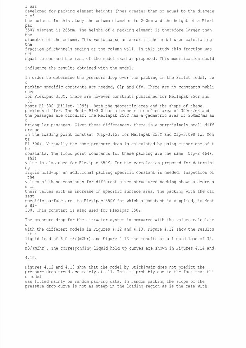
8/10/2019 Erasmus Mass 2004.PDF
http://slidepdf.com/reader/full/erasmus-mass-2004pdf 99/257
l wasdeveloped for packing element heights (hpe) greater than or equal to the diameter ofthe column. In this study the column diameter is 200mm and the height of a Flexipac350Y element is 265mm. The height of a packing element is therefore larger thanthediameter of the column. This would cause an error in the model when calculatingthefraction of channels ending at the column wall. In this study this fraction wassetequal to one and the rest of the model used as proposed. This modification could influence the results obtained with the model.
In order to determine the pressure drop over the packing in the Billet model, twopacking specific constants are needed, Clp and Cfp. There are no constants publishedfor Flexipac 350Y. There are however constants published for Mellapak 250Y and81Montz B1-300 (Billet, 1995). Both the geometric area and the shape of thesepackings differ. The Montz B1-300 has a geometric surface area of 300m2/m3 andthe passages are circular. The Mellapak 250Y has a geometric area of 250m2/m3 an
dtriangular passages. Given these differences, there is a surprisingly small differencein the loading point constant (Clp=3.157 for Mellapak 250Y and Clp=3.098 for MontzB1-300). Virtually the same pressure drop is calculated by using either one of theconstants. The flood point constants for these packing are the same (Cfp=2.464). Thisvalue is also used for Flexipac 350Y. For the correlation proposed for determiningliquid hold-up, an additional packing specific constant is needed. Inspection of the
values of these constants for different sizes structured packing shows a decrease intheir values with an increase in specific surface area. The packing with the closestspecific surface area to Flexipac 350Y for which a constant is supplied, is Montz B1-300. This constant is also used for Flexipac 350Y.
The pressure drop for the air/water system is compared with the values calculatedwith the different models in Figures 4.12 and 4.13. Figure 4.12 show the results at aliquid load of 6.0 m3/(m2hr) and Figure 4.13 the results at a liquid load of 35.
7m3/(m2hr). The corresponding liquid hold-up curves are shown in Figures 4.14 and 4.15.
Figures 4.12 and 4.13 show that the model by Stichlmair does not predict thepressure drop trend accurately at all. This is probably due to the fact that this modelwas fitted mainly on random packing data. In random packing the slope of thepressure drop curve is not as steep in the loading region as is the case with

8/10/2019 Erasmus Mass 2004.PDF
http://slidepdf.com/reader/full/erasmus-mass-2004pdf 100/257
structured packing. It performs reasonably well in predicting hold-up, especially athigh liquid loads (see Figure 4.15). The remaining three models predict the pressuredrop trend in the loading region. The Delft and SRP models predict the onset ofloading at lower vapour phase F-factors compared to the experimental data. TheDelft model predicts a higher pressure drop in the preloading region. The SRP modelaccurately predicts the pressure drop in the preloading region. At high liquid flowrates (Figure 4.13) the predicted slope of the pressure drop curve for the Delft andSRP models in the loading region is not as steep as was measured experimentally. Figures 4.12 and 4.13 show that the model by Billet tends to under predict thepressure drop in the preloading region slightly. It is accurate in predicting the loadingpoint and the slope of the pressure drop curve in the loading region.82
0200400600
8001000120014000 0.5 1 1.5 2 2.5 3 3.5 4 4.5FG [m/s.(kg/m3)0.5)]dP/dz [
Pa/m]experimentalSRPDelftStichlmairBillet Figure 4.12 Comparison between pressure drop calculated with semi-theoreticalmodels and experimental values. Flexipac 350Y, air/water system, uL,s=6.0
m3/(m2hr).02004006008001000120014000 0.5 1 1.5 2 2.5 3
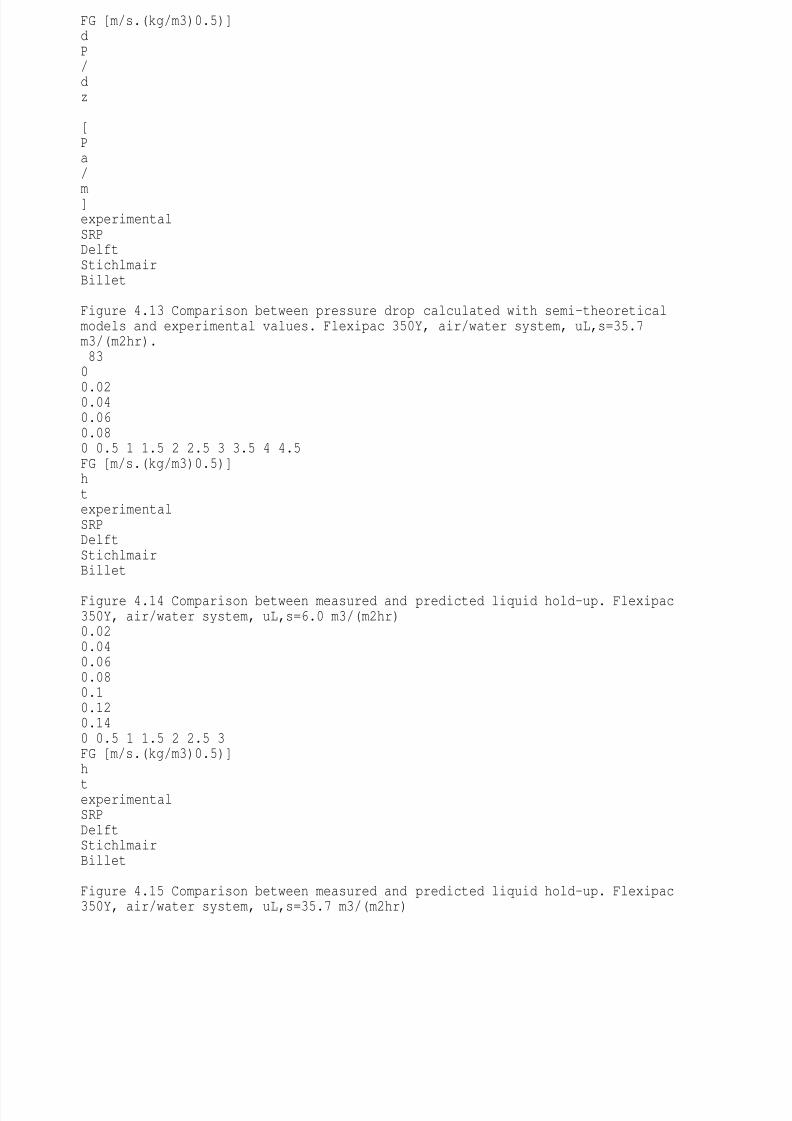
8/10/2019 Erasmus Mass 2004.PDF
http://slidepdf.com/reader/full/erasmus-mass-2004pdf 101/257
FG [m/s.(kg/m3)0.5)]dP/dz [Pa/m]experimentalSRPDelftStichlmairBillet Figure 4.13 Comparison between pressure drop calculated with semi-theoreticalmodels and experimental values. Flexipac 350Y, air/water system, uL,s=35.7m3/(m2hr).830
0.020.040.060.080 0.5 1 1.5 2 2.5 3 3.5 4 4.5FG [m/s.(kg/m3)0.5)]htexperimentalSRPDelftStichlmairBillet
Figure 4.14 Comparison between measured and predicted liquid hold-up. Flexipac350Y, air/water system, uL,s=6.0 m3/(m2hr)0.020.040.060.080.10.120.140 0.5 1 1.5 2 2.5 3FG [m/s.(kg/m3)0.5)]h
texperimentalSRPDelftStichlmairBillet Figure 4.15 Comparison between measured and predicted liquid hold-up. Flexipac350Y, air/water system, uL,s=35.7 m3/(m2hr)
8/10/2019 Erasmus Mass 2004.PDF
http://slidepdf.com/reader/full/erasmus-mass-2004pdf 102/257
84The Delft model assumes a constant liquid hold-up. Figure 4.14 and 4.15 show that itis rather accurate in the preloading region, but obviously fails to predict hold-up in theloading region. In this model the total surface area of the packing is assumed to bewetted. The SRP model predicts lower than measured liquid hold-up. It also fails topredict the right trend in the loading region. The experimental results of McNulty andHsieh (McNulty and Hsieh, 1982) formed a large portion of the data used indetermining the model constants. In this study the liquid hold-up is determinedbymeasuring the drop in the level of a recirculation tank. The system is calibrated byfirst operating the column without packing. The hold-up is then determined bysubtracting the hold-up in the system without packing from the hold-up measuredinthe system with packing. The hold-up determined in this way is smaller than thetruevalue. This is because for the empty column there is a volume of liquid free falling in
the column between the distribution point and the point where it is collected. Thecolumn is therefore not truly empty during calibration experiments. The modelbyBillet tends to under predict the liquid hold-up. It does however seem to predict theright trend of an increase in the hold-up in the loading region.
The pressure drop for the system air/Kerosol 200 is compared with the semi-theoretical models in Figure 4.16 and 4.17. Figure 4.16 show the results for a liquidload of 6.1 m3/(m2hr) and Figure 4.17 the results for a liquid load of 35.6 m3/(m2hr).
The corresponding hold-up curves are shown in Figures 4.18 and 4.19.
The model by Stichlmair again fails to predict the trend in the pressure drop curve.The SRP and Delft models predict the pressure drop in the preloading region with reasonable accuracy. The onset of loading conditions is predicted prematurely.Caution should however be exercised when using the SRP model for systems wherethe surface tension and viscosity differ from water. With the surface tension andviscosity shown in Table 4.1, a hold-up correction factor for partial wetting wascalculated to be approximately 4. This value is expected to be in the range 0-1
andwas subsequently set to unity. The model by Billet is again more accurate inpredicting the loading point compared to the other models. The predictions arehowever not as accurate as in the air/water system. At higher liquid loads (seeFigure4.17) the model predicts a lower than measured pressure drop in the preloadingregion.850200

8/10/2019 Erasmus Mass 2004.PDF
http://slidepdf.com/reader/full/erasmus-mass-2004pdf 103/257
4006008001000120014000 0.5 1 1.5 2 2.5 3 3.5 4FG [m/s.(kg/m3)0.5)]dP/dz [Pa/m]experimentalSRPDelftStichlmair
Billet Figure 4.16 Comparison between pressure drop calculated with semi-theoreticalmodels and experimental values. Flexipac 350Y, air/Kerosol 200 system, uL,s=6.1m3/(m2hr).0200400600800100012001400
0 0.5 1 1.5 2 2.5FG [m/s.(kg/m3)0.5)]dP/dz [Pa/m
]experimentalSRPDelftStichlmairBillet Figure 4.17 Comparison between pressure drop calculated with semi-theoreticalmodels and experimental values. Flexipac 350Y, air/Kerosol 200 system, uL,s=35.6

8/10/2019 Erasmus Mass 2004.PDF
http://slidepdf.com/reader/full/erasmus-mass-2004pdf 104/257
m3/(m2hr)8600.020.040.060.080.10.120 0.5 1 1.5 2 2.5 3 3.5 4FG [m/s.(kg/m3)0.5)]htexperimentalSRPDelftStichlmairBillet Figure 4.18 Comparison between measured and predicted liquid hold-up. Flexipac350Y, air/Kerosol 200 system, uL,s=6.1 m3/(m2hr)
0.040.06
0.080.10.120.140.160 0.5 1 1.5 2 2.5FG [m/s.(kg/m3)0.5)]htexperimentalSRPDelftStichlmair
Billet Figure 4.19 Comparison between measured and predicted liquid hold-up. Flexipac350Y, air/Kerosol 200 system, uL,s=35.6 m3/(m2hr)87Both the SRP and Delft models tend to over predict the liquid hold-up. At the highliquid load (Figure 4.19) the Delft models predicts the preloading liquid hold-upaccurately. The SRP model again fails to predict the steep increase in liquid hold-upin the loading region (Figure 4.18 and 4.19). The model by Billet predicts a too low
liquid hold-up, but predicts the correct trend in the loading region.
A comparison between the model predictions for the air/water and air/Kerosolsystems show that the semi-theoretical models show a conservative dependence ofcapacity on liquid viscosity.4.4.3 Implementation of models in design calculationsA column will typically be designed to operate in the region of the loading point. It istherefore important that any model accurately predicts the onset of loading conditions

8/10/2019 Erasmus Mass 2004.PDF
http://slidepdf.com/reader/full/erasmus-mass-2004pdf 105/257
and the pressure drop at this point. The next important parameter to be calculated isthe liquid hold-up at the loading point. The liquid hold-up will influence the effectivephase velocities and thus influence the calculated heat- and mass transfer rates
Of all the models evaluated in this study, the model of Stichlmair performed the worstoverall. This is, however, to be expected, since the bulk of the data used to fit themodel were for random packing. It does not predict the correct trend in the pressuredrop curve. It also tends to predict too low a liquid hold-up. The remainder ofthemodels performed reasonably well in predicting the loading point. The SRP modelisaccurate in predicting the loading point pressure drop. The Delft model prediction istoo high, while the Billet model prediction is too low. For predicting the pressure dropin the loading region, the model by Billet outperforms the SRP and Delft models. Although the Delft model does not predict the correct trend of the liquid hold-u
p in theloading region, it predicts the hold-up in the preloading region more accurately thanthe SRP or Billet models. The Billet model does however contain a packing specificconstant that was estimated in this study. Fitting the model to the experimental datawould obviously lead to an improvement in hold-up prediction by this model.
It would seem that a combination of the models should be used. In the preloading region up to the loading point, any of the models may be used. The Delft modelshould be preferred to calculate liquid hold-up and the SRP model will be more
accurate in predicting the loading point pressure drop. In the loading region, the Billetmodel is superior to the Delft and SRP models. The number of packing constantslimits the use of the Billet model. It does however provide an easy means to correlate88experimental data with. It is also demonstrated that the loading and flooding pointconstants are not packing specific and may be used for packing supplied by differentvendors. What is of importance though is the specific surface area of the packing.This will obviously apply to the normal capacity structured packing, and not the
highcapacity packing.
An advantage of any model would be versatility. High capacity packing is becomingincreasingly more popular and models need to be adapted to be able to predict theirperformance. Al the models rely on empirical correlations. It would therefore seemthat no model has a distinct advantage above another.

8/10/2019 Erasmus Mass 2004.PDF
http://slidepdf.com/reader/full/erasmus-mass-2004pdf 106/257
4.5 ConclusionsThe following conclusions may be drawn from the results obtained in this chapter forthe hold-up and pressure drop of Flexipac 350Y and Flexipac 350Y HC: The high capacity packing used in this study showed a higher dry bed pressuredrop compared with the normal capacity packing. This is due to the slightdifference in corrugation geometry between the two types of packing. There is an increase in capacity of 20% for the new packing compared with thenormal packing for the air/water system. The increase in capacity for theair/Kerosol 200 system is only 4%. The hydraulic capacity model by Stichlmair fails to predict the correct pressure drop trend. The SRP, Delft and Billet models perform reasonably well in predicting theloading point of the normal capacity packing. The model by Billet is more accurate in predicting steep slope of the pressuredrop curve in the loading region compared to the SRP and Delft models. The Delft model is more accurate than the SRP and Billet models in predictingthe hold-up in the preloading region. The SRP model should be used to predict pressure drop in the preloadingregion, as it is more accurate than the Billet and Delft models. All the models predict a conservative dependency of packing capacity on liquidviscosity.89
4.6 Nomenclatureae Effective surface area of packing [m2/m3]AG Channel area [m2]ah Specific hydraulic area [m2/m3]ap Geometric area of packing [m2/m3]B Channel base dimension [m]Bo Bond number [-]CL Liquid capacity factor [m/s]CG Vapour capacity factor [m/s]dc Diameter of column [m]dh Hydraulic diameter [m]dp Particle diameter [m]f Fraction of flooding [-]
f friction factor [-]FG Vapour phase load factor [(m/s)(kg/m3)0.5]Fload Pressure drop enhancement factor for loading region [-]Fp Packing factor [ft2/ft3]Fr Froude number [-]fs Wall factor [m]Ft Holdup correction factor for partial wetting [-]G Vapour mass flow rate [kg/s]g Gravitational acceleration [m/s2]geff Effective gravitational acceleration [m/s2]h Channel crimp height [m]hpb Height of a packed bed [m]hpe Height of a packing element [m]
ht Total liquid holdup [m3/m3]ht,0 Liquid holdup below the loading point [m3/m3]L Liquid mass flow rate [kg/s]Leq Equivalent length of channel [m]
G,pe Length of triangular vapour phase channel [m]NC Number of bends per unit height of packing [-]P Pressure [Pa]Re Reynolds number [-]S Channel side dimension [m]90
8/10/2019 Erasmus Mass 2004.PDF
http://slidepdf.com/reader/full/erasmus-mass-2004pdf 107/257
SG Dry channel perimeter [m]Si Wet channel perimeter [m]u Velocity [m/s]We Weber number [-]z Packing height [m]ze Inlet/exit calming section [m]Greekq Corrugation angle [o]m Dynamic viscosity [Pa.s]y Flow parameter [-]j Fraction of triangular passage occupied by liquid [-]y Fraction of vapour channels ending at column wall [-] (Delft model)d Liquid film thickness [m]d0 Liquid film thickness in absence of vapour flow [m]xbulk Direction change factor for bulk zone [-]xd Dry bed resistance factor [-]zDC Overall coefficient for direction change losses [-]xfp Flood point resistance factor [-]zGG Overall coefficient for vapour/vapour friction losses [-]xGG Vapour/vapour friction factor [-]zGL Overall coefficient for vapour/liquid friction losses [-]xGL Vapour/liquid friction factor [-]xlp Loading point resistance facto [-]e Void fraction [-]
g Contact angle between solid and liquid film [o]r Density [kg/m3]s Surface tension [N/m]t Shear stress [Pa]Subscriptsd Refers to dry bede Effectivefp Refers to flood pointG Refers to vapour phase propertyi Refers to vapour/liquid interface91irr Refers to irrigated (wetted) bedL Refers to liquid phase property
lp Refers to loading pointm Mean propertys Superficialw Refers to channel wallW Refers to property of water
925 MASS TRANSFER5.1 IntroductionThe HETP concept has been used to express the efficiency of column packing formany years (Sherwood et al., 1975). The limitations of this approach have long been
known (Chilton and Colburn, 1935). The HETP concept is sufficient to compare the performance of different types of structured packing with one another, as is oftendone in vendors brochures. But in order to use both the HTU/NTU method and thenon-equilibrium model, accurate mass transfer models and correlations are needed.In this chapter the different mass transfer correlations proposed for structured packing are presented and compared with one another. A simple, classical method

8/10/2019 Erasmus Mass 2004.PDF
http://slidepdf.com/reader/full/erasmus-mass-2004pdf 108/257
isused to measure vapour phase mass transfer coefficients in structured packing. Theuse of CFD to determine vapour phase mass transfer coefficients is demonstrated. The focus in this chapter is on vapour phase mass transfer, as it is widely acceptedthat the resistance in the vapour phase determines the overall mass transfer rate indistillation applications (Spiegel and Meier, 1987). Correlations proposed in literaturefor the liquid phase mass transfer coefficient in structured packing are alsodiscussed.5.2 Literature survey5.2.1 Literature ReviewThe first model proposed to determine the mass transfer coefficients in structuredpacking is that of Bravo et al. (Bravo et al., 1985). The model was developed forgauze-type structured packing where complete wetting of the packing surface isassumed. The relationship proposed by Johnstone and Pigford (Johnstone andPigford, 1942) for counter current evaporation in a wetted-wall column is used for thegas phase mass transfer coefficient with minor changes to the constants in the
correlation:0.8 0.333G G,e GSh 0.0338Re Sc= (5.1)The penetration theory of Higbie is used for the liquid side mass transfer coefficient:L L,eLD uk 2S= p (5.2)where the exposure time is taken as the time it takes for a fluid element to flowbetween corrugation channels. This distance is assumed to be equal to the93corrugation side length (S). The complete model (hydrodynamics and efficiency) i
sgiven in Appendix B.Spiegel and Meier (Spiegel and Meier, 1987) developed correlations for theperformance of the Mellapak range of corrugated sheet metal packing in the formofa series of graphs. The resistance to mass transfer in the liquid phase is assumed tobe much lower than the resistance to mass transfer in the vapour phase. For thegasphase the same proportionality as that proposed by Bravo et al. (Bravo et al., 1985)was found:0.8 0.333G G,e GSh Re Sc (5.3)
Rocha et al. (Rocha and Bravo, 1996) extended the model proposed by Bravo et al. (Bravo et al., 1985) to include sheet metal structured packing. The constants in thecorrelation for the gas phase mass transfer coefficient were changed slightly fromthat first suggested for gauze type packing. A packing specific constant was added inthe correlation for the liquid phase mass transfer coefficient. The effective surface
8/10/2019 Erasmus Mass 2004.PDF
http://slidepdf.com/reader/full/erasmus-mass-2004pdf 109/257
area is not assumed to be equal to the geometric surface area. The correlation byShi and Mersman (Shi and Mersmann, 1985) is used together with a factor thataccounts for surface texture to calculate the effective surface area. The completemodel is given in Appendix B. The mass transfer correlations are:( ) 0.8G,e L,e G 0.33G GGu u SSh 0.054 Sc + r =
m (5.4)9.0CwithduCD2kEhGe,LELL=p= (5.5)The model developed by Billet (Billet, 1995) focused primarily on random packing.The model was fitted on a large number of experimental data for distillation and
absorption and contains quite a number of packing specific constants. Constantsarealso available for a limited number of commercially available structured packing. Themodel is quite extensive and an attempt was made to highlight the most important equations in Appendix B. The correlation for the gas phase mass transfer coefficientis:=e -131.5p e34
G e G G G,s Gph ta a1k a C D Re Scad h (5.6)The correlation for the liquid phase mass transfer coefficient is split into two. Belowthe loading point:94
r= m 1 11 2 16 2 eL L6 3 3L e L p L,s
L h paDk a C g a ud a (5.7)Between the loading point and the flood point:
= 11 12 eL2 2L e L p L,eh p

8/10/2019 Erasmus Mass 2004.PDF
http://slidepdf.com/reader/full/erasmus-mass-2004pdf 110/257
aDk a 12 C a ud a (5.8)Laso et al. (Laso et al., 1995) measured the volumetric liquid side mass transfercoefficient (aekL) for the desorption of oxygen from water in a column equippedwithMellapak 250Y and 500Y. The proposed correlations are:= 0.62L e L,sk a 0.574u (Mellapak 250Y) (5.9)= 0.71L e L,sk a 0.713u (Mellapak 500Y) (5.10)The correlation for the liquid phase mass transfer coefficient of Brunazzi andPaglianti (Brunazzi and Paglianti, 1997) was fitted on experimental desorption andabsorption data using Mellapak 250Y and Sulzer BX packing. Data were obtained forthe desorption of CO2 from aqueous solutions and the absorption of chlorinatedcompounds into liquids of relative high viscosity and relative low surface tension. Thecorrelation was based on a proportionality proposed by Nawrocki and Chuang(Nawrocki and Chuang, 1996) who studied the absorption of carbon dioxide intostable rivulets on an inclined plate. Lower liquid phase mass transfer coefficientswere measured than predicted by the correlations of Bravo et al. (Bravo et al.,1985)and Billet (Billet, 1995). The mass transfer coefficients were higher than predi
cted bythe correlation of Laso et al. (Laso et al., 1995). The proposed correlation is: BL CGzSh AKa= (5.11)The definition of the Graetz (Gz) and Kapitsa (Ka) numbers are given in Appendix B.The constants in the correlation for Mellapak 250Y and Sulzer BX packing arepublished (Brunazzi and Paglianti, 1997).
In the model by Olujic (Olujic, 1997, Olujic et al., 1999) the vapour phase mass transfer coefficient is calculated as the average of laminar and turbulentcontributions.2 2G G,lam G,turbk k k= + (5.12)The laminar and turbulent mass transfer coefficients are obtained by invoking theheat/mass transfer analogy and using correlations for heat transfer:95= G,lam hG 1/ 3 hGG G,rG G,pek d d0.664Sc ReD (5.13)
( )x j
= +
x j + -
8/10/2019 Erasmus Mass 2004.PDF
http://slidepdf.com/reader/full/erasmus-mass-2004pdf 111/257
GL 2 / 3G,r GG,turb hG hGG G,pe2 / 3GLGRe Sck d d81D1 12.7 Sc 18 (5.14)Definitions for all the constants and dimensionless numbers may be obtained from Appendix B. The coefficient xGL is the so-called gas-liquid interaction coefficient. Theexpression for the liquid phase mass transfer coefficient is the same as thatproposed by Rocha et al. (Rocha and Bravo, 1996).
Weiland et al. (Weiland et al., 1993) studied the mass transfer characteristicsof twotypes of structured packing, Goodloe and Montz A2. The absorption of SO2 from airinto aqueous caustic soda solutions was used to determine the volumetric gas phasemass transfer coefficient (kGae). Interfacial area was measured by the absorption of
CO2 into dilute NaOH solutions. The volumetric liquid phase mass transfer coefficient(kLae) was measured by the absorption of CO2 into sodium carbonate/bicarbonatebuffer solutions. The results were correlated with a power law series containing therelevant dimensionless numbers. The experimental gas phase mass transfercoefficients were a factor 2 higher than calculated with the correlations proposed byBravo et al. (Bravo et al., 1985) for Sulzer BX packing. For the gas phase masstransfer the correlations are:= 1.10 1/ 3G G,s GSh 0.0567Re Sc (Goodloe packing) (5.15)= 1.02 1/ 3G G,s GSh 0.0373Re Sc (Montz A2) (5.16)The values for the liquid phase mass transfer coefficients were substantially lo
werthan that proposed by Bravo et al. (Bravo et al., 1985). The correlations for the twotypes of packing are:-= 0.08 1/ 2L L,s LSh 3.4Re Sc (Goodloe packing) (5.17)-= 0.04 1/ 2L L,s LSh 5.2Re Sc (Montz A2) (5.18)In a recent study, the evaporation of pure liquids in a short wetted-wall column wasused to develop a gas phase mass transfer correlation for structured packing(Crause and Nieuwoudt, 1999, Crause, 1998). The proposed correlation is:d= 0.5 0.08G p G,e G L,Sh 0.00283F Re Sc Re (5.19)96Liquid phase mass transfer was investigated by evaporating binary liquids. No li
quidside resistance was found but rather an enhancement of the gas phase masstransfer rate. By assuming complete wetting of the packing, the packing factor (Fp)for Mellapak 350Y in correlation 5.18 is Fp=1.03.The effect of the surface treatment of sheet metal structured packing on the gas phase mass transfer rate was investigated in a short wetted-wall column (Erasmus and Nieuwoudt, 2001, Erasmus, 1999). The proposed correlation is:

8/10/2019 Erasmus Mass 2004.PDF
http://slidepdf.com/reader/full/erasmus-mass-2004pdf 112/257
0.94 0.5G G,e GSh 0.0081Re Sc= (5.20)No liquid side resistance was found in the evaporation of binary liquids in thewetted-wall column.5.2.2 DiscussionThe major problem in developing correlations for the liquid and vapour mass transfercoefficients is that, in most experiments, volumetric transfer coefficients aremeasured (kLae and kGae). Since the effective surface area is thought to be mostlydependent on the liquid flow rate and the liquid properties, it would be logical toseparate the volumetric gas phase mass transfer coefficient into a gas phase masstransfer coefficient and an effective surface area. The gas phase mass transfercoefficient could then be correlated in terms of the gas phase flow rate and transportproperties.The wetted-wall analogy is often used to develop correlations for gas phase mass transfer in structured packing. It is convenient because the surface area is accuratelyknown and the gas phase mass transfer coefficient is therefore easily calculated from
experimental data. A large database of experimental data on the evaporation of purecomponents and binary mixtures in wetted-wall columns was compiled by Crauseand Nieuwoudt (Crause, 1998, Crause and Nieuwoudt, 1999), Erasmus andNieuwoudt (Erasmus, 1999, Erasmus and Nieuwoudt, 2001) and Kawesha andNieuwoudt. In all these studies, short wetted-wall columns were used. The reasoningbehind using a short column is that entrance effects should be considered indeveloping a correlation applicable to structured packing (Crause and Nieuwoudt, 1999) (Erasmus and Nieuwoudt, 2001). In structured packing the gas flow changesdirection quite often. This happens at the interface between packing elements and
also against the column wall. The liquid phase also changes direction where thecorrugations of opposing sheets meet. In all three studies, a long gas phase entrancelength to the wetted-wall column is allowed. The velocity boundary layer wouldtherefore be completely developed before reaching the wetted-wall section. In the97wetted wall section a concentration boundary layer would then start to develop butwould not develop fully because of the short length of the wetted-wall section.Abetter approach would probably be not to allow a velocity boundary layer to develop
before reaching the wetted-wall section. This would be more representative of theflow conditions inside structured packing where a fully developed velocity profilewould not be attained due to the number of abrupt changes in the flow path(channels). Another problem with applying a wetted-wall analogy is that the flow isessentially two dimensional in a wetted-wall column while it is essentially threedimensional in structured packing.
8/10/2019 Erasmus Mass 2004.PDF
http://slidepdf.com/reader/full/erasmus-mass-2004pdf 113/257
In the correlation proposed by Olujic et al. (Olujic et al., 1999) (Equations 5.12-5.14)the analogy between heat- and mass transfer is used. The proposed correlation is analogous to correlations developed for heat transfer in tubes with developingthermal and velocity boundary layers (entrance region). This correlation wouldtherefore also tend to under predict the mass transfer rate in structured packingbecause it does not take the three-dimensional nature of the flow into account.In studies on compact heat exchangers (Focke et al., 1985) and rotary air preheaters(Ciofalo et al., 1996, Ciofalo, 1996, Stasiek et al., 1996) the heat/mass transfer rateswere found to be enhanced by the swirling motion induced in the flow by the free shear layer at the open interface between two flow channels. These heat exchangershave a geometry quite similar to structured packing. This is especially the case withthe rotary air heat exchanger investigated by Stasiek et al. (Stasiek et al., 1996).Correlations developed for heat transfer could be used to predict mass transferinstructured packing by invoking the analogy between heat- and mass transfer.
Unfortunately most of the results from this study are proprietary in nature andnotpublished in the open literature.In the model by Rocha et al. (Rocha and Bravo, 1996, Rocha et al., 1993) the wettedarea of the packing are modelled by using a correlation similar to that proposed byShi and Mersmann (Shi and Mersmann, 1985). The constants in this correlation are obtained by fitting experimental hold-up data. With the wetted surface area known,the liquid phase mass transfer coefficient is modelled with the penetration theory of
Higbie. The surface renewal time are determined by fitting the penetration model toexperimental data for the desorption of oxygen from water. With the wetted areaandthe liquid phase mass transfer coefficient known, the gas phase mass transfercoefficient is the only unknown and is determined from experimental distillation data.The problem with this model is that the wetted area is assumed to be equal to thesurface area effectively taking part in mass transfer. It has been known for quitesome time that the wetted area is not necessarily equal to the effective mass transfer
98area in columns with random packing (Danckwerts, 1970). Any errors made indetermining the surface area, and assuming aw=ae, will propagate through the modeland lead to an inaccurate determination of the gas phase mass transfer coefficient.In the remaining models, the gas- or liquid phase volumetric mass transfercoefficients are measured (Brunazzi and Paglianti, 1997, Brunazzi et al., 1995,Lasoet al., 1995, Weiland et al., 1993) using either physical or chemical

8/10/2019 Erasmus Mass 2004.PDF
http://slidepdf.com/reader/full/erasmus-mass-2004pdf 114/257
absorption/desorption. In almost all of these studies aqueous systems were used. These systems have high surface tensions and are notorious for their low wetting ability (Rocha and Bravo, 1996). It is therefore not surprising that the results differconsiderably from one another. Another factor that will influence the experimentalresults for the liquid phase mass transfer coefficient considerably is the estimation ofthe binary diffusion coefficient in the liquid phase. No mention is usually made ofphysical models used to calculate the diffusion coefficient.In the present study it is argued that one should first measure the gas phase masstransfer coefficient independently and then use the resulting model or correlation as astarting point for measuring effective surface area and the liquid phase mass transfercoefficient. This could be done by measuring mass transfer coefficients underconditions where the total geometric surface area of the packing contributes tothemass transfer process. Heat transfer rates could also be measured and the masstransfer rates obtained by invoking the heat-/mass transfer analogy. The
naphthalene/air system was chosen in this study. It has been used in the past to determine the gas phase mass transfer coefficient and wetted area in randompacking (Shulman et al., 1955). There are also accurate data available for vapourpressure (Ambrose et al., 1975) and the diffusion coefficient of naphthalene into air(Cho et al., 1992). In the rest of this chapter the experimental set-up and results fornaphthalene sublimation from the surface of structured packing with a geometrysimilar to Flexipac 350Y is discussed. This is followed by CFD simulation of the results. The measurement and correlation of the liquid phase mass transfer
coefficient is not investigated. The focus of the study is on the modelling of distillationin structured packing. The general view is that the mass transfer rate is determinedby the resistance in the gas phase.5.3 TheoryThe diffusion of a species away from a liquid-gas or solid-gas interface into the gasphase may be described by diffusion through a stagnant gas, also known as Stefan diffusion (Coulson and Richardson, 1991). In the following derivation species Awill99
be the component that evaporates/sublimes and species B will be the gas. Accordingto Fick
s law, the respective diffusion rates of species A and species B are:AA AB t dyN D cdx= - (5.21)andBB BA t dyN D cdx= - (5.22)Because the mole fractions of the two components sum to unity:A By y 1+ = (5.23)

8/10/2019 Erasmus Mass 2004.PDF
http://slidepdf.com/reader/full/erasmus-mass-2004pdf 115/257
the diffusion rate for species B may be written as:( ) ( )A AB AB t AB td 1 y d yN D c D cdx dx-= - = (5.24)The total mass transfer rate of species B is zero. There must therefore be a bulk flowof the system to the interface to counterbalance the diffusion flux away from theinterface. For species B:( ) ( )B B BT BFN N N 0= + = (5.25)Therefore:( ) AB B AB tBF dyN N D c dx= - = - (5.26)The bulk flow of a will be yA/yB that of the bulk flow of B:( ) ( )A A AA B AB tBF BFB By y dyN N D cy y dx
= = - (5.27)The total mass transfer rate for species A is therefore:( ) A A AA AB t AB tTB B
y dy dy1N 1 D c D cy dx y dx = - + = - (5.28)Integration over the film thickness yields:( )= - - tABA A,b A,iB,mcDN y yy (5.29)where yB,m is the logarithmic mean defined by:B,b B,iB,m B,bB,i
y yyylny-= (5.30)In keeping with the definition of a mass transfer coefficient given in chapter 2,Equation 5.29 is written as:100( )tA G A,b A,iB,mcN k y yy= - - (5.31)5.3.1 Naphthalene sublimation in structured packing
For naphthalene the sublimation rate is small so that yB,m»1. In order to obtain thetotal mass transfer rate in the column, the following integration has to be performed:( )h 2 rA A P G t A,i A,b0 0 0n N A a k c y y rdrd dzp= = - q (5.32)where aP is the specific surface area of the coated packing. If it is assumed that thevariables are independent of r and q (good radial distribution), the pressure drop isnegligible (ct is constant) and that kG is uniform over the height of the column

8/10/2019 Erasmus Mass 2004.PDF
http://slidepdf.com/reader/full/erasmus-mass-2004pdf 116/257
, thenEquation 5.31 reduces to:( )h2A P G t A,i A,b0n a k c r y y dz= p - (5.33)A log-mean driving force is used:( ) ( )( )( )A,i A,b A,i A,bh 0AA,i A,b hA,i A,b 0y y y yyy yln y y- - -D = -
- (5.34)The total mass transfer rate of A is therefore:2A G t P AG t P C An k c a r h y
k c a V y= p D= D (5.35)where VC is the volume of the test section in the column.The vapour phase mass transfer coefficient is then calculated from:AGt P C Ankc a V y= D (5.36)To calculate the driving force in Equation 5.36, the interface concentration ofspeciesA is needed. If the saturated vapour pressure of species A at the interface is k
nown,the interface mole fraction may simply be calculated from:satAA,iTPyP= (5.37)5.3.2 Evaporation in a wetted wall columnIn a wetted wall column where the concentration of the evaporating species in thegas layer next to the interface is high, the effects of bulk flow may not be ignored. Todetermine the mass transfer rate, the following integration has to be performed:
101( )h 2 tA A i G A,i A,b0 0B,mcn N A k y y rd dzyp= = - q (5.38)If a short column is employed the effects of evaporative cooling may be ignoredandyA,i will be constant along the length of the column. If it is assumed that the
8/10/2019 Erasmus Mass 2004.PDF
http://slidepdf.com/reader/full/erasmus-mass-2004pdf 117/257
variablesare independent of q, the mass transfer rate may be determined from:tA i G AB,mcn A k yy= D (5.39)where the area of the interface is calculated with:iA 2 rh= p (5.40)A logarithmic average of the inlet and outlet driving force is used (Equation 5.34). Fora short column, an arithmic mean between the inlet and outlet may be used for yB,m inEquation 5.39. With the mass transfer rate known, the vapour phase mass transfer coefficient is determined from Equation 5.39.5.4 Experimental5.4.1 Experimental set-upThe experimental set-up was the same as described in Chapter 4. The naphthalene-coated packing section was sandwiched between two normal Flexipac 350Y packingelements with an element height of 265mm. The packing elements were rotated 90owith respect to one another. The top of the packed bed was situated just below thetop flange of the glass column section. This was achieved by using a spacer on top
of the static mixer. The spacer was constructed in a manner so as not to obstruct theairflow into the passages of the bottom packing element. The column was operated at ambient conditions. The outlet section of the column was fastened in a manner tofacilitate quick removal.5.4.2 Naphthalene coatingWire gauze packing was used for the naphthalene coated test section. Preliminary coating tests showed that a smooth and consistent coating could be obtained with wire gauze packing. Coatings applied to sheet metal structured packing tend to c
rackand flake off. The coatings applied to the wire gauze packing were resistant toacertain amount of deformation of the packing. The packing had the same channeldimensions as Flexipac 350Y. The element height was considerably shorter at166mm. The packing was not perforated. The packing element was disassembled inorder to coat each corrugated wire gauze sheet individually. Before the coating102procedure each sheet was washed in acetone and left to dry. Only half of the sheetwas coated. This made it both easier to coat the packing by a dipping procedureandalso ensured that the outlet of the packed section was far from being saturated
withnaphthalene. If the concentration of the air at the outlet of the test section is close tothe saturation concentration, then the driving force for mass transfer will vanish. Thenaphthalene used for the coating had a purity of 99%. Each sheet was weighedbefore it was coated. This was done to ensure that a coating of similar thickness wasapplied on each sheet. Each sheet was measured in order to calculate the surface

8/10/2019 Erasmus Mass 2004.PDF
http://slidepdf.com/reader/full/erasmus-mass-2004pdf 118/257
area accurately. The packing was then coated by dipping it repeatedly into moltennaphthalene kept at a temperature of 85oC. The container with molten naphthalene was submerged into a thermostat controlled water bath. After each dipping the sheetwith naphthalene coating was left to cool and dry (solidify) for a few moments beforeapplying the next layer of coating. In between coating layers the packing wasweighed. This was done to determine when a sufficiently thick coating had beenapplied. After a sheet had been coated it was transferred to a container with an airtight lid. Fine naphthalene crystals at the bottom of the container ensured a saturated naphthalene atmosphere inside the container. After all the sheets hadbeencoated, the packing element was again reconstructed from the different sheets. Wirewas used to bind the sheets together. In order for the coated packing element to fitinto the column, the two outermost sheets had to be discarded. The loss in surfacearea due to this action was taken into account. A bit of the coating along the side of
the sheets were damaged in the binding process. A brush was used to dislodge any loose pieces of coating. Before the element was weighed, it was inserted into adiethat had the same ID as the column. During this operation any of the sharpnaphthalene edges protruding from the packing was broken off. The element wasthen removed from the die and any lose naphthalene pieces was shaken out andbrushed off. The element was then weighed and transferred back to the airtightcontainer. After a few experimental runs, the coating had to be re-applied. Theonlyway in which a uniform coating could be obtained was to first remove the old coating.This was done by submerging the sheets into the molten naphthalene container unt
ilthe naphthalene melted. Increasing the temperature of the naphthalene bath duringthis stage to 90oC accelerated the process. The coating procedure was thenrepeated, starting with an acetone wash to remove any remaining naphthalene. The uncoated element weighed approximately 740g. The total mass of naphthalenecoated onto the packing varied between 330g and 410g. Table 5.1 show the average dimensions of the coated naphthalene packing section.103Table 5.1 Dimensions of naphthalene coated packing sectionProperty Value
Corrugation base, B [mm] 17.4Corrugation side, S [mm] 11.2Crimp height, h [mm] 7.05Void fraction, e 0.87Corrugation angle, q [o] 45Height of coated section [mm] 835.4.3 Experimental procedureThe naphthalene coated packing section was accurately weighed before eachexperimental run. It was then carefully transferred to the packed bed. It was inserted

8/10/2019 Erasmus Mass 2004.PDF
http://slidepdf.com/reader/full/erasmus-mass-2004pdf 119/257
into the packed bed with the coated section facing either downwards or upwards.Theblower was switched on and the temperature of the air before and after the columnwas logged, together with the pressure drop over the orifice plate and atmosphericpressure. After a suitable amount of time, determined by the airflow rate and thetemperature, the blower was switched of and the naphthalene-coated section wasremoved and weighed. The experimental time varied between 20 and 50 minutesresulting in naphthalene mass losses of between 10g and 40g. After weighing thecoated packing element, the element was disassembled and each sheet was visually inspected and weighed. If the coating was found to be too thin on the sheets, thesheets were recoated.5.5 Results and discussion5.5.1 Experimental resultsThe mass loss of naphthalene was converted to a mass transfer coefficient usingEquation 5.35. The vapour pressure of naphthalene was calculated using the dataofAmbrose et al. (Ambrose et al., 1975). This data was also used in a recent study onthe diffusion of naphthalene through air (Cho et al., 1992). The vapour pressure
isobviously quite sensitive to temperature. The influence of temperature on the resultswill be discussed in the next section. In Figure 5.1 an average temperature wasusedbetween the inlet and outlet of the column. The average difference between the inletand outlet temperatures was 0.9oC. The results are presented as a plot of kG againstthe Reynolds number. The Reynolds number used in the plots is the effectiveReynolds number defined as:104G G,e h
G,eGu dRe r=m (5.41)The effective velocity of the air is calculated from:= e qG,sG,e uu sin (5.42)where uG,s is the superficial air velocity based on the column cross sectional area, e isthe void fraction of the naphthalene coated test section and q is the packingcorrugation angle with respect to the horizontal axis. Since the sublimation rate waslow, the density at the outlet was calculated as that of air. The transport properties of
air were taken from literature (Incropera and De Witt, 1990). The hydraulic diameter(dh) was calculated for a unitary
criss-cross
cell. According to the definition of thehydraulic diameter (Daugherty and Franzini, 1977):hw4V BhdA S= = (5.43)B, h and S are the base, side and height of a naphthalene coated triangular pass
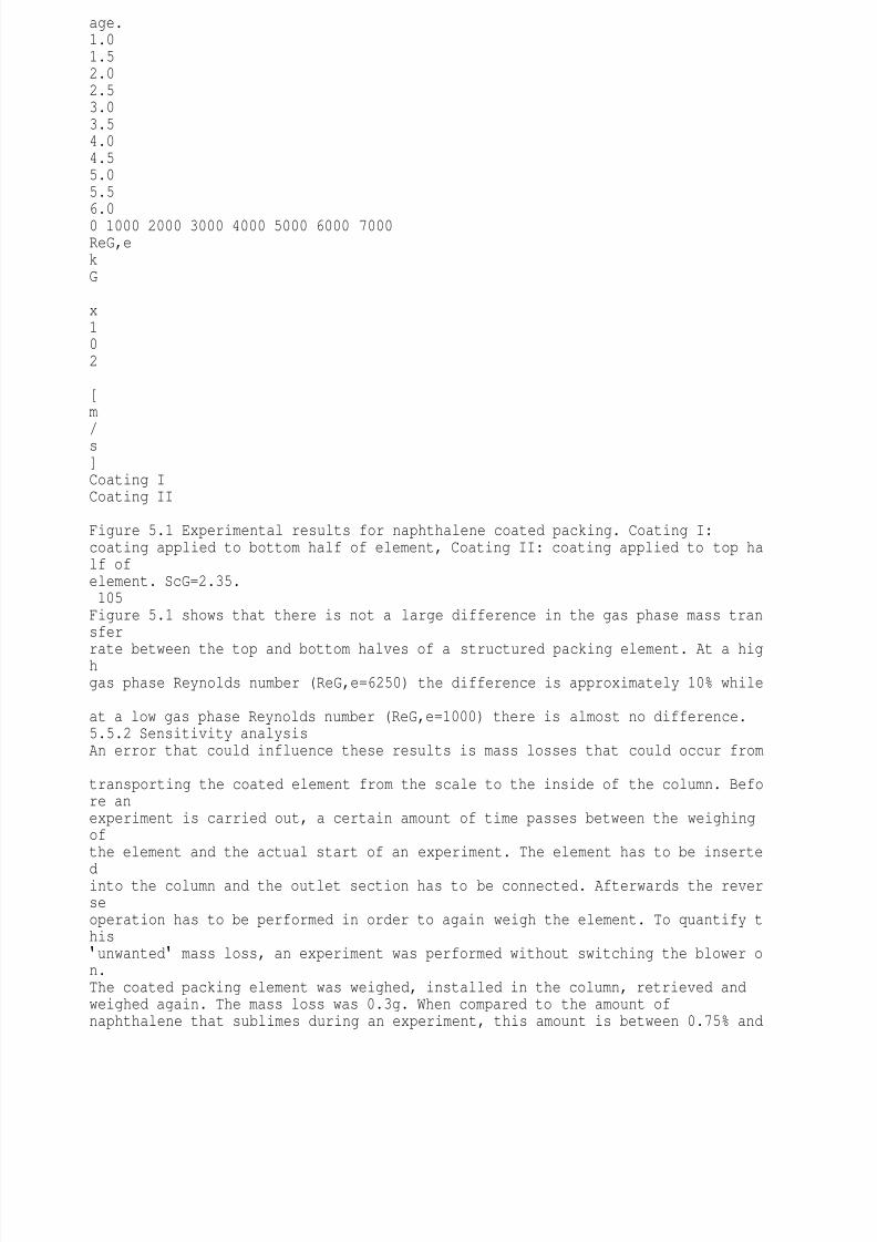
8/10/2019 Erasmus Mass 2004.PDF
http://slidepdf.com/reader/full/erasmus-mass-2004pdf 120/257
age.1.01.52.02.53.03.54.04.55.05.56.00 1000 2000 3000 4000 5000 6000 7000ReG,ekG x102 [m
/s]Coating ICoating II Figure 5.1 Experimental results for naphthalene coated packing. Coating I:coating applied to bottom half of element, Coating II: coating applied to top half ofelement. ScG=2.35.105Figure 5.1 shows that there is not a large difference in the gas phase mass transfer
rate between the top and bottom halves of a structured packing element. At a highgas phase Reynolds number (ReG,e=6250) the difference is approximately 10% while at a low gas phase Reynolds number (ReG,e=1000) there is almost no difference.5.5.2 Sensitivity analysisAn error that could influence these results is mass losses that could occur from transporting the coated element from the scale to the inside of the column. Before anexperiment is carried out, a certain amount of time passes between the weighingofthe element and the actual start of an experiment. The element has to be inserte
dinto the column and the outlet section has to be connected. Afterwards the reverseoperation has to be performed in order to again weigh the element. To quantify this
unwanted mass loss, an experiment was performed without switching the blower on.The coated packing element was weighed, installed in the column, retrieved andweighed again. The mass loss was 0.3g. When compared to the amount ofnaphthalene that sublimes during an experiment, this amount is between 0.75% and

8/10/2019 Erasmus Mass 2004.PDF
http://slidepdf.com/reader/full/erasmus-mass-2004pdf 121/257
3.0% of the total mass lost. When subtracting this amount from the total andrecalculating the mass transfer coefficients, the average difference between the corrected and uncorrected values is 1.4%. Since some of the experiments wereperformed on cooler days the unwanted mass loss should be less than the 0.3gfound on a warm day and the average difference substantially lower than thecalculated 1.4%. The unwanted mass loss would then approach the accuracy of thescale (0.1g). It was subsequently decided to ignore this error.A second and more serious error could result from the accuracy of the temperaturemeasurements. The inlet and outlet temperature was measured with class B PT100sensors. For these sensors the maximum deviation at the experimental conditionsis
0.4oC. If this amount is subtracted from the average temperature (average between inlet and outlet) and then used to recalculate the mass transfer coefficients, then theirvalues are on average 4.5% lower. If the average temperature is lowered by 0.4oC and the mass transfer coefficients recalculated, then the value is on average 4.8%higher. The experimental error in the data represented in Figure 5.1 is therefore
estimated to be in the order of 5%.5.5.3 Comparison with existing correlationsCorrelations used to calculate the gas phase mass transfer coefficient in structuredpacking are given in Table 5.1. The correlation in the Delft (Olujic, 1997) modelcontains liquid/vapour interaction terms and was omitted for obvious reasons. The106correlation proposed by Billet (Billet, 1995) is also not included since no parametersfor Flexipac 350Y (or Mellapak) could be found. The correlation by Gilliland and
Sherwood (Gilliland and Sherwood, 1934) is also givenTable 5.2 Correlations for the gas phase mass transfer coefficient in Figure 5.2 Correlation Reference0.8 0.333G G,e GSh 0.0338Re Sc= (Bravo et al., 1985)0.8 0.33G G,e GSh 0.054Re Sc= (Rocha and Bravo,1996)0.978 0.532G G,e GSh 0.00526Re Sc= (Crause andNieuwoudt, 1999)0.94 0.5G G,e GSh 0.0081Re Sc= (Erasmus andNieuwoudt, 2001)
The correlation proposed by Rocha et al. (Rocha and Bravo, 1996) is frequently u
sedand often referenced in the literature (Fair et al., 2000, Brunazzi and Paglianti, 1997,De Brito et al., 1994, Shetty and Cerro, 1997). The remaining correlations are wettedwall based correlations. The correlations from Crause and Nieuwoudt (Crause andNieuwoudt, 1999) and Erasmus and Nieuwoudt (Erasmus and Nieuwoudt, 2001)given in Table 5.1 are those that do not contain a liquid term. The correlationproposed by Bravo et al. (Bravo et al., 1985) is also included. These correlations are

8/10/2019 Erasmus Mass 2004.PDF
http://slidepdf.com/reader/full/erasmus-mass-2004pdf 122/257
compared with the experimental results in Figure 5.2. This figure show that allthecorrelations underestimate the gas phase mass transfer coefficient. The correlationproposed by Rocha et al. (Rocha and Bravo, 1996) and used in the SRP model (Fair et al., 2000) estimates mass transfer coefficients that are considerably closerto theexperimental points than the other correlations shown in the figure.
1070.01.02.03.04.05.06.00 1000 2000 3000 4000 5000 6000 7000 8000ReG,ekG x
102 [m/s]BravoRochaCrause & NieuwoudtErasmus & Nieuwoudt
Coating ICoating II Figure 5.2 Comparison between experimental results and existing kG correlations. 5.5.4 Correlation of experimental resultsThe experimental data are correlated with a simple power law series similar to thatused in the other correlations:b cG G,e GSh aRe Sc= (5.44)Since only air was used in the experiments, some assumption regarding thedependency of the mass transfer coefficient on the Schmidt number (and therefore
the diffusion coefficient) must be made. This is done in order to extrapolate thecorrelation to systems other than air/naphthalene. In most mass transfer correlationsfor the evaporation of liquids in a wetted wall column, the Schmidt number is raisedto a power of between 0.33 and 0.5. This suggests the following dependency of themass transfer coefficient on the diffusion coefficient:2 3Gk D for 1 3G GSh Sc (5.45)

8/10/2019 Erasmus Mass 2004.PDF
http://slidepdf.com/reader/full/erasmus-mass-2004pdf 123/257
Gk D for 0.5G GSh Sc (5.46)In a recent publication (Dudukovic et al., 1996) it is suggested that for fluid-fluidtransfer, the Schmidt number should be raised to the power 0.5 and for solid-fluid108transfer to the power 0.33. These suggestions are based on a model for the turbulentviscosity near the liquid-gas interface (free surface) proposed by Levich (Levich,1962). For wetted-wall experimental data the accuracy of the correlation was slightlyimproved by setting the Schmidt number coefficient equal to 0.5 (kG D0.5). Thetheory on which their suggestion is based is for the transport of a species from thebulk fluid phase to the free surface. Since all the experimental data that are referredto are for the evaporation of pure components in a wetted wall column, transport inthe liquid phase should not be considered at all. There are quite a few analyticalmodels and expressions proposed for the turbulent transport of heat and mass nearinterfaces (Sideman and Pinczewski, 1975). For turbulent transport at interfaces
influids with molecular Prandtl/Schimdt numbers close to unity, there is little differencebetween the different theories. It is only at Prandtl/Schimdt numbers considerablysmaller and larger than one that these models differ from one another. In most of themodels the Prandtl/Schimdt number is raised to the power 0.33-0.5. For distillationand absorption the gas phase Schmidt number would be in the range 0.5<Sc<5. It istherefore expected that by choosing either 0.33 or 0.5 would not influence thecalculated mass transfer coefficient to a significant extent. The experimental d
atawere fitted to Equation 5.43 using both 0.5 and 0.33 (kG D0.5 and kG D0.67). The datawere regressed by using non-linear least square minimization. The regression resultsfor the correlations are given in Table 5.2.Table 5.3 Regression results for naphthalene sublimation dataCorrelation RMS*0.62 0.5G G,e GSh 0.2641Re Sc= 2.834 (5.47)0.62 0.33G G,e GSh 0.3053Re Sc= 2.836 (5.48)( )2exp calcnSh Sh
*RMS n-=
Figure 5.3 shows a parity plot of the values predicted by Correlation 5.47 and 5.48against the experimental values.1091

8/10/2019 Erasmus Mass 2004.PDF
http://slidepdf.com/reader/full/erasmus-mass-2004pdf 124/257
234561 2 3 4 5 6kGx102 [m/s] (experimental)kGx102 [m/s] (pre
dicted) Figure 5.3 Parity plot of mass transfer coefficients predicted with correlation5.47and 5.48 against experimental values.As mentioned before, it was found that by assuming kG D0.5 resulted in a marginally
better fit of the correlation on the experimental results for wetted-wall columns(Dudukovic et al., 1996). A wetted-wall type correlation has been used in the past forgas phase mass transfer in structured packing (Bravo et al., 1985) (Rocha andBravo, 1996). In this correlation kG D0.67 (see Table 5.1). This is also the case for kGcorrelations proposed by Billet (Billet, 1995) for random and structured packing. Thiscorrelation has been fitted on a large set of experimental data. It would seem thatexperimental evidence suggests a kG D0.67 dependency in distillation and absorption.
This dependency is also used in the remainder of this study. It should however betested experimentally by varying the Schmidt number in sublimation experiments.One possible way is to use the sublimation of benzoic acid into air. It is a convenientsystem because benzoic acid is not toxic and inexpensive. Another possibility is touse naphthalene but with a different carrier gas. The experiments would, however,then have to be performed on a much smaller scale since it would be quite expens
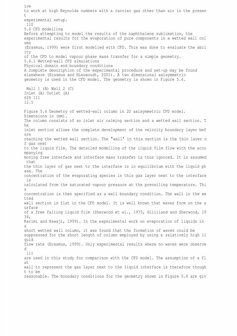
8/10/2019 Erasmus Mass 2004.PDF
http://slidepdf.com/reader/full/erasmus-mass-2004pdf 125/257
iveto work at high Reynolds numbers with a carrier gas other than air in the presentexperimental setup.1105.6 CFD modellingBefore attempting to model the results of the naphthalene sublimation, theexperimental results for the evaporation of pure components in a wetted wall column(Erasmus, 1999) were first modelled with CFD. This was done to evaluate the abilityof the CFD to model vapour phase mass transfer for a simple geometry.5.6.1 Wetted-wall CFD simulationsPhysical domain and boundary conditionsA complete description of the experimental procedure and set-up may be foundelsewhere (Erasmus and Nieuwoudt, 2001). A two dimensional axisymmetricgeometry is used in the CFD model. The geometry is shown in Figure 5.4.
Wall 1 (B) Wall 2 (C)Inlet (A) Outlet (A)628 11112.5
Figure 5.4 Geometry of wetted-wall column in 2D axisymmetric CFD model.
Dimensions in (mm).The column consists of an inlet air calming section and a wetted wall section. Theinlet section allows the complete development of the velocity boundary layer beforereaching the wetted wall section. The wall in this section is the thin layer of gas nextto the liquid film. The detailed modelling of the liquid film flow with the accompanyingmoving free interface and interface mass transfer is thus ignored. It is assumed thatthe thin layer of gas next to the interface is in equilibrium with the liquid phase. The
concentration of the evaporating species in this gas layer next to the interface iscalculated from the saturated vapour pressure at the prevailing temperature. Thisconcentration is then specified as a wall boundary condition. The wall in the wettedwall section is flat in the CFD model. It is well known that waves form on the surfaceof a free falling liquid film (Sherwood et al., 1975, Gilliland and Sherwood, 1934,Karimi and Kawaji, 1999). In the experimental work on evaporation of liquids inashort wetted wall column, it was found that the formation of waves could be
suppressed for the short length of column employed by using a relatively high liquidflow rate (Erasmus, 1999). Only experimental results where no waves were observed111are used in this study for comparison with the CFD model. The assumption of a flatwall to represent the gas layer next to the liquid interface is therefore thought to bereasonable. The boundary conditions for the geometry shown in Figure 5.4 are giv
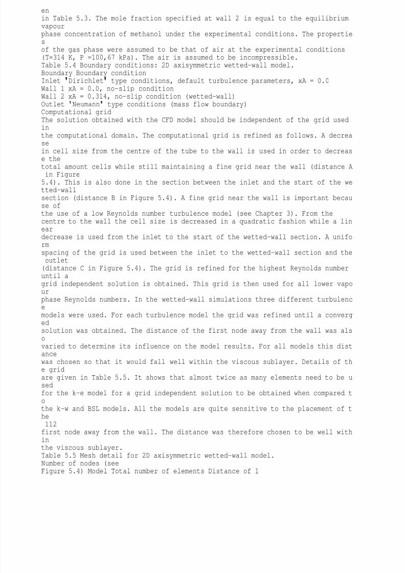
8/10/2019 Erasmus Mass 2004.PDF
http://slidepdf.com/reader/full/erasmus-mass-2004pdf 126/257
enin Table 5.3. The mole fraction specified at wall 2 is equal to the equilibriumvapourphase concentration of methanol under the experimental conditions. The propertiesof the gas phase were assumed to be that of air at the experimental conditions(T=314 K, P =100,67 kPa). The air is assumed to be incompressible.Table 5.4 Boundary conditions: 2D axisymmetric wetted-wall model.Boundary Boundary conditionInlet
Dirichlet
type conditions, default turbulence parameters, xA = 0.0Wall 1 xA = 0.0, no-slip conditionWall 2 xA = 0.314, no-slip condition (wetted-wall)Outlet Neumann type conditions (mass flow boundary)Computational gridThe solution obtained with the CFD model should be independent of the grid usedinthe computational domain. The computational grid is refined as follows. A decreasein cell size from the centre of the tube to the wall is used in order to decrease thetotal amount cells while still maintaining a fine grid near the wall (distance A in Figure5.4). This is also done in the section between the inlet and the start of the wetted-wall
section (distance B in Figure 5.4). A fine grid near the wall is important because ofthe use of a low Reynolds number turbulence model (see Chapter 3). From thecentre to the wall the cell size is decreased in a quadratic fashion while a lineardecrease is used from the inlet to the start of the wetted-wall section. A uniformspacing of the grid is used between the inlet to the wetted-wall section and the outlet(distance C in Figure 5.4). The grid is refined for the highest Reynolds numberuntil agrid independent solution is obtained. This grid is then used for all lower vapour
phase Reynolds numbers. In the wetted-wall simulations three different turbulencemodels were used. For each turbulence model the grid was refined until a convergedsolution was obtained. The distance of the first node away from the wall was alsovaried to determine its influence on the model results. For all models this distancewas chosen so that it would fall well within the viscous sublayer. Details of the gridare given in Table 5.5. It shows that almost twice as many elements need to be usedfor the k-e model for a grid independent solution to be obtained when compared t
othe k-w and BSL models. All the models are quite sensitive to the placement of the112first node away from the wall. The distance was therefore chosen to be well withinthe viscous sublayer.Table 5.5 Mesh detail for 2D axisymmetric wetted-wall model.Number of nodes (seeFigure 5.4) Model Total number of elements Distance of 1

8/10/2019 Erasmus Mass 2004.PDF
http://slidepdf.com/reader/full/erasmus-mass-2004pdf 127/257
st nodefrom wall [mm]A B CLaminar 9000 0.15 30 200 111k-e 16800 0.005 55 200 111k-w 9000 0.005 30 200 111BSL 9000 0.005 30 200 111Mathematical models and computational detailsChapter 3 may be consulted for details on the turbulence models and the governingequations of fluid motion. The default turbulence parameters for each of theturbulence models are given in Appendix A. Hybrid differencing was used for allvariables with the SIMPLEC algorithm to solve the pressure velocity coupling. Steadystate simulations were performed with under relaxation to control the rate ofconvergence. A simulation was judged to have reached convergence when theglobal mass source residual was less than 10-6.Results and discussionThe mass transfer rate is determined from the outlet concentration of the
evaporating
species. Equation 5.38 is used to calculate a mass transfer coefficient.The results for the different turbulence models are compared with the experimentalresults in Figure 5.5. Details of the computational grid that resulted in a conv
ergedsolution are given in Table 5.4 for each turbulence model used. Figure 5.5 showtheexpected trend for laminar and turbulent flow. At low gas phase Reynolds numbers,the flow is in the laminar regime and the mass transfer rate is predicted withreasonable accuracy by a laminar model (ReG<2500). At higher Reynolds numbersthe laminar model predicts lower than measured mass transfer rates. The BSL modelof Menter fails to predict the mass transfer rate up to a gas phase Reynolds ofabout4000. Above ReG=4000 it is more accurate than the other turbulence models. The k-e
and k-w models give almost identical results over the entire range. The fine gridneeded for a converged solution to be obtained for the k-e model would limit its application in problems with larger computational domains. This was indeed113experienced when attempting to model the naphthalene sublimation results asdescribed in the following section.
0.511.52
2.50 1500 3000 4500 6000ReGkGx102
8/10/2019 Erasmus Mass 2004.PDF
http://slidepdf.com/reader/full/erasmus-mass-2004pdf 128/257
[m/s]experimentallaminark-epsilonk-omegaBSL Figure 5.5 CFD results for wetted-wall evaporation. ReG for experimental results is relative to moving liquid interface, ReL(exp)=285.5.6.2 CFD modelling of naphthalene sublimationThe breakdown of a bed of structured packing into re-occurring micro elements is discussed in detail in Chapter 3. From a mass transfer point of view the mostimportant micro element is the junction between two corrugated passages, alsoreferred to as micro element 2 in Chapter 3. When calculating the pressure dropovera bed of packing, the contributions from the other elements are also important sincethey involve the abrupt change in the flow direction of the vapour phase. It is
therefore easy to construct simplified geometries that represent this directionchange.Whether these simplified geometries will also be accurate for modelling masstransfer is questionable. In this study the contributions to mass transfer fromthesemicro elements are assumed to be equal to the contribution from the micro elementformed at the junction between corrugated channels. These elements may be usedto reconstruct the bulk of the packing by arranging a number of them in series.114Physical domain and boundary conditionsThere are different geometries used in the literature (Ciofalo et al., 1996, Hodson,
1997, Hodson et al., 1997, Larachi et al., 2003, Petre et al., 2003) to represent there-occurring micro element in cross-corrugated passages. In earlier studies (Hodsonet al., 1997, Ciofalo et al., 1996) the inlet and oulet sections to these microelementsare next to the free shear plane formed at the open interface between corrugated channels. In a recent study on pressure drop in structured packing (Petre et al.,2003), these inlet- and outlet boundaries are moved a distance away from the freeshear interface. The reasoning behind this extension is that a developed flow pr
ofileis assumed when applying boundary conditions at an inlet- and outlet boundary. Byplacing an inlet- or an outlet boundary close to the free shear interface, these boundary conditions will be violated. In a study where these boundaries were placednext to the free shear interface, the results obtained agreed with experimentaldata(Ciofalo et al., 1996). This was also the case for results obtained with boundar

8/10/2019 Erasmus Mass 2004.PDF
http://slidepdf.com/reader/full/erasmus-mass-2004pdf 129/257
iesremoved from the free shear interface (Petre et al., 2003). In this study, boththeseapproaches are followed and compared with experimental results. Figure 5.6 shows details of the physical domain. The physical domain where the inlet- and outletboundaries are moved up- and downstream from the free shear interface will bereferred to as geometry 1. For this geometry the distance f in Figure 5.6 (a) is greaterthan zero. The physical domain where the inlet and outlet boundaries are next to thefree shear interface will be referred to as geometry 2. For this geometry the distance fin Figure 5.6 (a) is equal to zero. The average dimensions of the naphthalene-coatedchannels are used in constructing the geometry. The properties used are that ofairand naphthalene at the experimental conditions and are listed in Table 5.6. Theair isassumed to be incompressible. The boundary conditions are shown in Table 5.7.Table 5.6 Properties of air/naphthalene systemProperty Units Valuer [kg/m3] 1.162DAB [m2/s] 6.72·10-6
m [Pa.s] 1.85·10-5Psat(naphthalene) [Pa] 14.5
Dirichlet boundary conditions are specified at the inlet boundaries. For the first microelement a uniform inlet velocity profile is specified normal to the boundary interface.The outlet from the first micro element is used as the inlet to the next micro element.The mass flow boundary specified at the outlets imposes Neumann boundary115conditions on all the variables (see Chapter 3). A complete developed flow profile is
assumed when imposing this boundary condition. All transported variables, except the components of velocity, are given zero gradients normal to the boundary.fINLET INLETOUTLETOUTLETcdeab(a)(b)
Figure 5.6 Computational domain. (a) Top view of cross-corrugated channels. (b)View of inlet- and outlet boundary, dimensions in [mm].The gradients for the velocity components are set equal to a constant value,calculated from global mass convergence considerations. The distance that the outletboundaries are moved down stream from the free shear interface must therefore be sufficient to allow any recirculation vortex to get completed before reaching the outletboundary. This distance was found to be equal to the length of the base of a cha
8/10/2019 Erasmus Mass 2004.PDF
http://slidepdf.com/reader/full/erasmus-mass-2004pdf 130/257
nnel17.4 f4.7 e2.35 d17.4 c5.6 b5.6 a116(distance c in Figure 5.6) by Petre et al. (Petre et al., 2003). This distance is alsoused in this study. Simulations where this distance was set equal to half the length ofthe corrugation base (distance c in Figure 5.6) failed to converge. An extra conditionimposed on the outlet boundaries is that of equal flux splitting. The mass flowisdivided equally between the two outlet boundaries. A constant mass fraction isspecified against the walls in the section where the two triangular channels meet.This mass fraction is calculated from the naphthalene vapour pressure at theexperimental conditions. The vapour pressure of naphthalene is calculated with theequation proposed by Ambrose et al. (Ambrose et al., 1975). For the geometry where
the inlet and outlet boundaries are removed from the free shear interface (geometry1), an extra wall boundary condition is imposed. The bottom wall of the channelleading up the free shear interface is specified to be a free slip boundary (see Figure5.6). A velocity boundary layer is therefore not allowed to develop next to this wall.On all the remaining walls a no-slip condition is imposed.Table 5.7 Boundary conditions for micro elementBoundary Boundary conditionInlets 1 & 2 Dirichlet type boundary condition, default turbulence parameters,
xA = 0.0Wall (1) xA = 6.4·10-4, no-slip conditionWall (2)* free slip conditionOutlets 1 & 2
Neumann
type boundary condition*This boundary is only present if distance f > 0 (see Figure 5.6)Computational gridIn order to generate a rectangular structured grid (see Chapter 3), the triangularpassages are divided into three rectangular blocks (shown in Figure 5.6). The use ofa low Reynolds number turbulence model requires a fine grid in the near wall region.In order to use the minimum amount of volume elements while still maintaining a
finegrid near the wall, a quadratic decrease in grid spacing is used from the middle of thepassage to the wall (distance a in Figure 5.6). A fine grid is also necessary in theregion of the free shear interface. The properties of the flow will change overshortdistances in this region. A quadratic decrease in cell size is used between themiddleof the passage and the free shear interface (distance b in Figure 5.6). For the

8/10/2019 Erasmus Mass 2004.PDF
http://slidepdf.com/reader/full/erasmus-mass-2004pdf 131/257
geometries where the inlet and outlet boundaries are placed a distance away from the free shear interface, the grid is also quadratically expanded from the freeshearinterface to the outlet boundary (distance f in Figure 5.6). The same procedurewas117used to obtain a grid independent solution as discussed in the previous section. Thegrid is refined for the highest Reynolds number until a grid independent solution isobtained. This grid is then used for all lower Reynolds numbers. For both geometriesthe first grid point was placed at a distance of 0.01 mm away from the wall boundary.At the highest gas phase Reynolds number (ReG » 6200), this distance translatedinto an average dimensionless distance away from the wall of y+» 0.18 for geometry 1 and y+» 0.23 for geometry 2. This is well within the viscous sublayer of theboundary layer. This distance was also use for all lower Reynolds numbers. Detailsof the converged grid for the two geometries are given in Table 5.8. The numberofnode points on distance b was reduced to 20 for geometry 1 in order to reduce th
etotal number of volume elements. Doing so did not influence the solution. When thenumber of nodes were reduced from 30 to 20 for geometry 2, there was a significantchange in the solution.Table 5.8 Details of converged grid for packing micro elementNumber of nodes* Geometrya b FDistance 1st nodefrom wall [mm]Total number ofvolume elements
1 30 20 40 0.01 540 0002 30 30 n/a 0.01 290 000* See Figure 5.6 for descriptionMathematical model and computational detailsThe k-w and BSL turbulence model were used. Chapter 3 may be consulted fordetails on these turbulence models and the governing equations of fluid motion.Hybrid differencing was used for all variables with the SIMPLEC algorithm to solvethe pressure-velocity coupling. Steady state simulations were performed with acombination of false time stepping and under relaxation to control the rate ofconvergence. A simulation was judged to have reached convergence when theglobal mass source residual was less than 10-6.Results and discussion
The sublimation rate of naphthalene is determined by simulating the airflow through amicro element and calculating the difference in concentration of naphthalenebetween the inlet and outlet boundaries. A mass transfer coefficient is calculated withEquation 5.35 for each micro element and the gas phase Reynolds number iscalculated using Equation 5.40. Seven micro elements in series are modelled. Thiscorresponds to the longest channel found in the coated structured packing element.

8/10/2019 Erasmus Mass 2004.PDF
http://slidepdf.com/reader/full/erasmus-mass-2004pdf 132/257
118
In preliminary runs both the k-w and BSL turbulence models were used. From Figure5.5 it would seem that the k-w model should be used at low Reynolds numbers (uptoabout ReG 4000) and the BSL model for Reynolds numbers ReG > 4000. In thesepreliminary runs a normal no-slip boundary was specified on the bottom wall of thechannel leading into and out of the `criss-cross' element (geometry 1). The totalnumber of elements was also less than shown in Table 5.8. (332 000 volumeelements). Figure 5.7 show the results obtained with the two turbulence models.Themass transfer coefficient shown is the average calculated for the seven microelements. Figure 5.7 show that the same result is obtained with the two turbulencemodels at low Reynolds numbers (ReG < 4000). At high Reynolds numbers (ReG >4000) the BSL model predicts a higher mass transfer rate compared to the k-wmodel.01234
560 2000 4000 6000 8000ReGkGx102 [m
/s]BSLk-omega Figure 5.7 Mass transfer coefficients calculated at different ReG with the k-w andBSL turbulence models.In subsequent simulations only the BSL turbulence model was used since it gave thesame result at low Reynolds numbers compared to the k-w model. It is also expected
(see Figure 5.5) that the BSL model will be more accurate than the k-w model athighReynolds numbers (ReG > 4000).
Figure 5.8 show the results obtained for the micro element where the boundariesarelocated next to the free shear interface (geometry 2). The results shown in this figure119were obtained with the BSL turbulence model. Details of the converged grid are
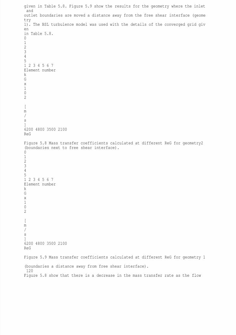
8/10/2019 Erasmus Mass 2004.PDF
http://slidepdf.com/reader/full/erasmus-mass-2004pdf 133/257
given in Table 5.8. Figure 5.9 show the results for the geometry where the inlet andoutlet boundaries are moved a distance away from the free shear interface (geometry1). The BSL turbulence model was used with the details of the converged grid givenin Table 5.8.0123451 2 3 4 5 6 7Element numberkGx102 [m
/s]6200 4800 3500 2100ReG Figure 5.8 Mass transfer coefficients calculated at different ReG for geometry2(boundaries next to free shear interface).01234
51 2 3 4 5 6 7Element numberkGx102 [m/
s]6200 4800 3500 2100ReG Figure 5.9 Mass transfer coefficients calculated at different ReG for geometry 1 (boundaries a distance away from free shear interface).120Figure 5.8 show that there is a decrease in the mass transfer rate as the flow
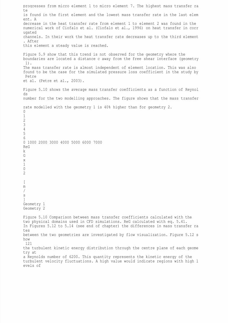
8/10/2019 Erasmus Mass 2004.PDF
http://slidepdf.com/reader/full/erasmus-mass-2004pdf 134/257
progresses from micro element 1 to micro element 7. The highest mass transfer rateis found in the first element and the lowest mass transfer rate in the last element. Adecrease in the heat transfer rate from element 1 to element 2 was found in thenumerical work of Ciofalo et al. (Ciofalo et al., 1996) on heat transfer in corrugatedchannels. In their work the heat transfer rate decreases up to the third element. Afterthis element a steady value is reached.
Figure 5.9 show that this trend is not observed for the geometry where theboundaries are located a distance c away from the free shear interface (geometry 1).The mass transfer rate is almost independent of element location. This was alsofound to be the case for the simulated pressure loss coefficient in the study by Petreet al. (Petre et al., 2003).
Figure 5.10 shows the average mass transfer coefficients as a function of Reynoldsnumber for the two modelling approaches. The figure shows that the mass transfer rate modelled with the geometry 1 is 40% higher than for geometry 2.
01234560 1000 2000 3000 4000 5000 6000 7000ReGkGx1
02 [m/s]Geometry 1Geometry 2 Figure 5.10 Comparison between mass transfer coefficients calculated with thetwo physical domains used in CFD simulations. ReG calculated with eq. 5.41.
In Figures 5.12 to 5.14 (see end of chapter) the differences in mass transfer ratesbetween the two geometries are investigated by flow visualization. Figure 5.12 show121the turbulent kinetic energy distribution through the centre plane of each geometry ata Reynolds number of 6200. This quantity represents the kinetic energy of theturbulent velocity fluctuations. A high value would indicate regions with high levels of
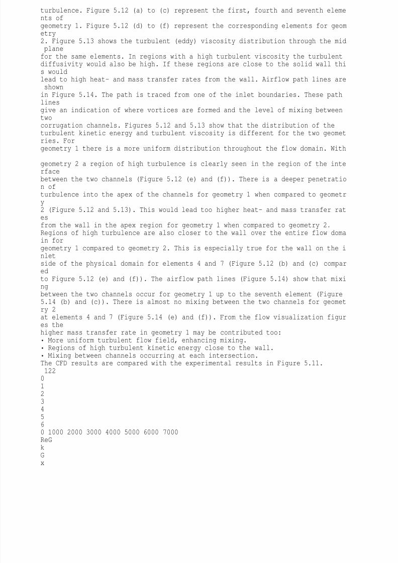
8/10/2019 Erasmus Mass 2004.PDF
http://slidepdf.com/reader/full/erasmus-mass-2004pdf 135/257
turbulence. Figure 5.12 (a) to (c) represent the first, fourth and seventh elements ofgeometry 1. Figure 5.12 (d) to (f) represent the corresponding elements for geometry2. Figure 5.13 shows the turbulent (eddy) viscosity distribution through the mid planefor the same elements. In regions with a high turbulent viscosity the turbulentdiffusivity would also be high. If these regions are close to the solid wall this wouldlead to high heat- and mass transfer rates from the wall. Airflow path lines are shownin Figure 5.14. The path is traced from one of the inlet boundaries. These pathlinesgive an indication of where vortices are formed and the level of mixing betweentwocorrugation channels. Figures 5.12 and 5.13 show that the distribution of theturbulent kinetic energy and turbulent viscosity is different for the two geometries. Forgeometry 1 there is a more uniform distribution throughout the flow domain. With geometry 2 a region of high turbulence is clearly seen in the region of the interfacebetween the two channels (Figure 5.12 (e) and (f)). There is a deeper penetration of
turbulence into the apex of the channels for geometry 1 when compared to geometry2 (Figure 5.12 and 5.13). This would lead too higher heat- and mass transfer ratesfrom the wall in the apex region for geometry 1 when compared to geometry 2.Regions of high turbulence are also closer to the wall over the entire flow domain forgeometry 1 compared to geometry 2. This is especially true for the wall on the inletside of the physical domain for elements 4 and 7 (Figure 5.12 (b) and (c) comparedto Figure 5.12 (e) and (f)). The airflow path lines (Figure 5.14) show that mixing
between the two channels occur for geometry 1 up to the seventh element (Figure5.14 (b) and (c)). There is almost no mixing between the two channels for geometry 2at elements 4 and 7 (Figure 5.14 (e) and (f)). From the flow visualization figures thehigher mass transfer rate in geometry 1 may be contributed too: More uniform turbulent flow field, enhancing mixing. Regions of high turbulent kinetic energy close to the wall. Mixing between channels occurring at each intersection.The CFD results are compared with the experimental results in Figure 5.11.12201
234560 1000 2000 3000 4000 5000 6000 7000ReGkGx
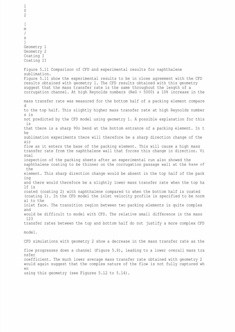
8/10/2019 Erasmus Mass 2004.PDF
http://slidepdf.com/reader/full/erasmus-mass-2004pdf 136/257
102 [m/s]Geometry 1Geometry 2Coating ICoating II Figure 5.11 Comparison of CFD and experimental results for naphthalenesublimation.Figure 5.11 show the experimental results to be in close agreement with the CFDresults obtained with geometry 1. The CFD results obtained with this geometrysuggest that the mass transfer rate is the same throughout the length of acorrugation channel. At high Reynolds numbers (ReG > 5000) a 10% increase in the mass transfer rate was measured for the bottom half of a packing element comparedto the top half. This slightly higher mass transfer rate at high Reynolds number
s isnot predicted by the CFD model using geometry 1. A possible explanation for this isthat there is a sharp 90o bend at the bottom entrance of a packing element. In thesublimation experiments there will therefore be a sharp direction change of theairflow as it enters the base of the packing element. This will cause a high masstransfer rate from the naphthalene wall that forces this change in direction. Visualinspection of the packing sheets after an experimental run also showed thenaphthalene coating to be thinner on the corrugation passage wall at the base of the
element. This sharp direction change would be absent in the top half of the packingand there would therefore be a slightly lower mass transfer rate when the top half iscoated (coating 2) with naphthalene compared to when the bottom half is coated(coating 1). In the CFD model the inlet velocity profile is specified to be normal to theinlet face. The transition region between two packing elements is quite complexandwould be difficult to model with CFD. The relative small difference in the mass123transfer rates between the top and bottom half do not justify a more complex CFD
model.
CFD simulations with geometry 2 show a decrease in the mass transfer rate as the flow progresses down a channel (Figure 5.8), leading to a lower overall mass transfercoefficient. The much lower average mass transfer rate obtained with geometry 2would again suggest that the complex nature of the flow is not fully captured whenusing this geometry (see Figures 5.12 to 5.14).

8/10/2019 Erasmus Mass 2004.PDF
http://slidepdf.com/reader/full/erasmus-mass-2004pdf 137/257
An advantage of the CFD simulations using geometry 1 is that only a single elementneeds to be modelled in order to predict the mass transfer rate for a whole packingelement with reasonable accuracy. In future this would reduce the computationaleffort immensely.5.7 ConclusionsFrom the experimental investigation of the gas phase mass transfer in structured packing, the following conclusions may be drawn: Current wetted-wall type correlations predict lower than measured gas phasemass transfer coefficients in Flexipac 350Y. Naphthalene sublimation experiments performed with Flexipac 350Y led to thefollowing correlations for the gas phase mass transfer rate:0.62 0.5G G,e GSh 0.2641Re Sc=0.62 0.33G G,e GSh 0.3053Re Sc= The gas phase mass transfer rate was found to be the same for the bottom- andtop half of a structured packing element. Results from the CFD simulations of the gas phase mass transfer rate instructured packing show that: The BSL turbulence model of Menter (Menter, 1994) may be used to predict thegas phase mass transfer rate in structured packing. The results obtained are sensitive to the placement of inlet- and outlet
boundaries. These boundaries should be moved away from the open free shearinterface between two corrugated channels. A distance equal to the corrugationbase was found to be adequate (See Figure 5.6). Only a single representative micro element needs to be modelled to determinethe overall mass transfer rate with reasonable accuracy.124
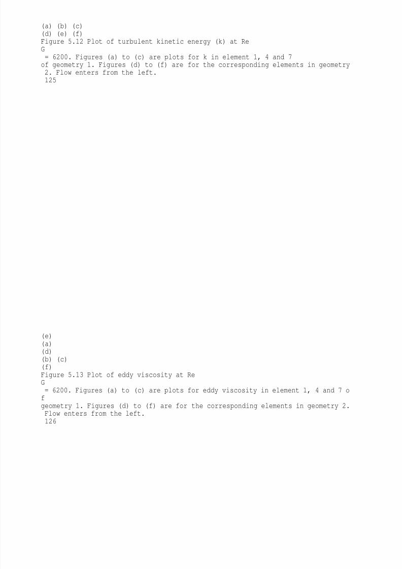
8/10/2019 Erasmus Mass 2004.PDF
http://slidepdf.com/reader/full/erasmus-mass-2004pdf 138/257
(a) (b) (c)(d) (e) (f)Figure 5.12 Plot of turbulent kinetic energy (k) at ReG = 6200. Figures (a) to (c) are plots for k in element 1, 4 and 7of geometry 1. Figures (d) to (f) are for the corresponding elements in geometry 2. Flow enters from the left.125
(e)(a)(d)(b) (c)(f)Figure 5.13 Plot of eddy viscosity at ReG = 6200. Figures (a) to (c) are plots for eddy viscosity in element 1, 4 and 7 o
fgeometry 1. Figures (d) to (f) are for the corresponding elements in geometry 2. Flow enters from the left.126
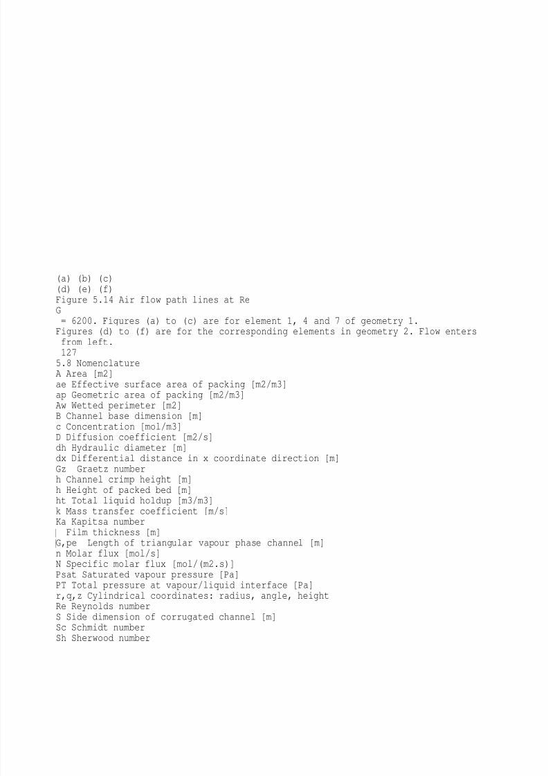
8/10/2019 Erasmus Mass 2004.PDF
http://slidepdf.com/reader/full/erasmus-mass-2004pdf 139/257
(a) (b) (c)(d) (e) (f)Figure 5.14 Air flow path lines at ReG = 6200. Figures (a) to (c) are for element 1, 4 and 7 of geometry 1.Figures (d) to (f) are for the corresponding elements in geometry 2. Flow enters from left.1275.8 NomenclatureA Area [m2]ae Effective surface area of packing [m2/m3]ap Geometric area of packing [m2/m3]
Aw Wetted perimeter [m2]B Channel base dimension [m]c Concentration [mol/m3]D Diffusion coefficient [m2/s]dh Hydraulic diameter [m]dx Differential distance in x coordinate direction [m]Gz Graetz numberh Channel crimp height [m]h Height of packed bed [m]ht Total liquid holdup [m3/m3]k Mass transfer coefficient [m/s]Ka Kapitsa number
Film thickness [m]
G,pe Length of triangular vapour phase channel [m]n Molar flux [mol/s]N Specific molar flux [mol/(m2.s)]Psat Saturated vapour pressure [Pa]PT Total pressure at vapour/liquid interface [Pa]r,q,z Cylindrical coordinates: radius, angle, heightRe Reynolds numberS Side dimension of corrugated channel [m]Sc Schmidt numberSh Sherwood number

8/10/2019 Erasmus Mass 2004.PDF
http://slidepdf.com/reader/full/erasmus-mass-2004pdf 140/257
u Velocity [m/s]Vc Volume of packed bed [m3]x Mass fraction in vapour phase [-]y Mole fraction in vapour phase [-]yB,m Logarithmic mean mole fraction [-]y+ Dimensionless distance128Greekp = 3.14159¼q Corrugation angle [o]m Dynamic viscosity [Pa.s]j Fraction of triangular passage occupied by liquid [-]xGL Vapour/liquid friction factor [-]e Void fraction [-]r Density [kg/m3]SubscriptsA Refers to component Ab Refers to bulk of phaseB Refers to component BBF Refers to
bulk flow
molar fluxe EffectiveG Refers to vapour phase propertyi Refers to vapour/liquid interfaceL Refers to liquid phase property
s SuperficialT Refers to total molar flux
1296 EFFECTIVE INTERFACIAL AREA6.1 IntroductionThe efficiency of structured packing depends strongly on the effective interfacial areafor gas phase mass transfer between the liquid and vapour phases. This quantityis,however, difficult to measure and conflicting results were obtained by different
studies on effective interfacial area in the past (Weimer and Schaber, 1997, DeBritoet al., 1994). When determining the effective interfacial area in structured packing,aqueous systems have almost exclusively been used. Aqueous systems arenotorious for their bad wetting characteristics of stainless steel surfaces. Inthischapter the use of an organic system to determine effective interfacial area ofFlexipac 350Y is explored.6.2 Literature survey6.2.1 Definitions of effective interfacial areaThere are quite a few definitions for interfacial area in a packed column. Shi and
Mersmann (Shi and Mersmann, 1985) lists these as: Actual interfacial area between gas and liquid (ai) Interfacial area between packing and liquid (aw) Active interfacial area for gas phase mass transfer (aG) Active interfacial area for liquid phase mass transfer (aL) Active interfacial area for evaporation (aV) Active interfacial area for mass transfer accompanied by a chemical reaction(aC).The term effective interfacial area could therefore refer to aG, aL, aV or ac, depending
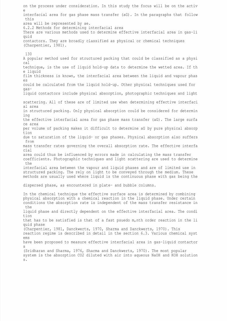
8/10/2019 Erasmus Mass 2004.PDF
http://slidepdf.com/reader/full/erasmus-mass-2004pdf 141/257
on the process under consideration. In this study the focus will be on the activeinterfacial area for gas phase mass transfer (aG). In the paragraphs that follow thisarea will be represented by ae.6.2.2 Methods for determining interfacial areaThere are various methods used to determine effective interfacial area in gas-liquidcontactors. They are broadly classified as physical or chemical techniques(Charpentier, 1981).
130A popular method used for structured packing that could be classified as a physicaltechnique, is the use of liquid hold-up data to determine the wetted area. If the liquidfilm thickness is known, the interfacial area between the liquid and vapour phasescould be calculated from the liquid hold-up. Other physical techniques used forgas-liquid contactors include physical absorption, photographic techniques and light scattering. All of these are of limited use when determining effective interfacial area
in structured packing. Only physical absorption could be considered for determiningthe effective interfacial area for gas phase mass transfer (aG). The large surface areaper volume of packing makes it difficult to determine aG by pure physical absorptiondue to saturation of the liquid- or gas phases. Physical absorption also suffers frommass transfer rates governing the overall absorption rate. The effective interfacialarea could thus be influenced by errors made in calculating the mass transfercoefficients. Photographic techniques and light scattering are used to determine the
interfacial area between the vapour and liquid phases and are of limited use instructured packing. The rely on light to be conveyed through the medium. Thesemethods are usually used where liquid is the continuous phase with gas being the dispersed phase, as encountered in plate- and bubble columns.
In the chemical technique the effective surface area is determined by combiningphysical absorption with a chemical reaction in the liquid phase. Under certainconditions the absorption rate is independent of the mass transfer resistance in theliquid phase and directly dependent on the effective interfacial area. The conditionthat has to be satisfied is that of a fast psuedo m,nth order reaction in the li
quid phase(Charpentier, 1981, Danckwerts, 1970, Sharma and Danckwerts, 1970). Thisreaction regime is described in detail in the section 6.3. Various chemical systemshave been proposed to measure effective interfacial area in gas-liquid contactors(Sridharan and Sharma, 1976, Sharma and Danckwerts, 1970). The most popularsystem is the absorption CO2 diluted with air into aqueous NaOH and KOH solutions.
8/10/2019 Erasmus Mass 2004.PDF
http://slidepdf.com/reader/full/erasmus-mass-2004pdf 142/257
In the following section the use of physical and chemical methods to determineeffective interfacial area in structured packing and the correlations proposed byvarious investigators are discussed.6.2.3 Interfacial area in structured packingIn the model by Billet (Billet, 1995) the effective interfacial area is assumedto beequal to the interfacial area between the vapour and the liquid. At the loadingpoint itis calculated with:131- - = e
0.5 0.2 0.75 0.45e L,s L,s L,sp lpa 3 Re We Fra (6.1)The effective interfacial area between the load- and flood point is calculated with anexpression similar to that for hold-up (see Chapter 4) in the loading region:( ) ( )G,s G,s lp13G,se e e ep p p p G,su u lp fp lp fp
ua a a aa a a a u> = + -

8/10/2019 Erasmus Mass 2004.PDF
http://slidepdf.com/reader/full/erasmus-mass-2004pdf 143/257
(6.2)with the effective interfacial area at the flood point calculated from:0.56e eLp W pfp lpa a7a a
s= s (6.3)For negative surface tension gradient systems in distillation applications, theeffectivesurface area is reduced by surface destabilization:( )0.54e eLp pnega a1 2.4 10 Maa a- = -
(6.4)where MaL is the Marangoni number defined by:D=mL L L p
xMaD a (6.5)The methodology used to arrive at these expressions are not clearly stated (Billet,1995).
It is common practice to assume that the effective interfacial area is equal tothewetted surface area. In the model proposed by Bravo et al. (Bravo et al., 1985)forgauze packing, complete wetting of the packing is assumed. The wetted area isassumed to be equal to the effective interfacial area, and is taken to be equalto the
geometric area of the packing:e w pa a a= = (6.6)For gauze packing this may be a reasonable approximation. For sheet metalstructured packing the packing surface may not be completely wetted and Fair and Bravo (Fair and Bravo, 1990) suggests incorporating a discount factor in calculatingthe effective surface area from the packing surface area:e pa a= b (6.7)where0.50 0.0058 (%flood)b = + · (6.8)132Shi and Mersmann (Shi and Mersmann, 1985) developed an expression for the
wetted surface area for a liquid flowing down an inclined plate. Rocha et al. (Rocha etal., 1993, Rocha and Bravo, 1996) used this expression to correlate experimental hold-up and efficiency data for structured packing. This resulted in the followingequation to calculate the ratio of effective- to geometric surface area:( )( )( )= e - g q0.15 0.359

8/10/2019 Erasmus Mass 2004.PDF
http://slidepdf.com/reader/full/erasmus-mass-2004pdf 144/257
L,s L,seSE 0.30.2 0.6p L,s29.12 We Fr Sa Fa Re 1 0.93cos sin (6.9)The factor FSE accounts for the surface treatment of the packing (lancing, fluting,embossing etc.). The wettability of the surface is accounted for by the contactangleg.
Nawrocki et al. (Nawrocki et al., 1991) developed a detailed liquid distribution modelto determine the wetted area in structured packing. According to the model, a volumeof liquid (or rivulet) flowing in a channel is split up into two equal portionsat anintersection point. A portion of the liquid continues down the same channel while theother portion flows down through the intersection point into the next channel. Thesplit ratio is assumed to be uniform through the packing and is determined by fittingthe model to experimental hold-up data. The model uses the correlation proposed
byShi and Mersmann (Shi and Mersmann, 1985) to determine the rivulet width. Theeffective surface area is assumed to be equal to the wetted surface area and may therefore be calculated from the rivulet width in each section of the packing.
Brunazzi et al. (Brunazzi et al., 1995) proposed an expression for the ratio oftheeffective interfacial area to geometric area. The equation is based on the classicallaminar falling film thickness for a liquid flowing down an inclined tube and the liquidhold-up calculated with a suitable correlation:
0.51.5e hG t Lp L L,sa d h gsin sina 4 3 u
r q e q = e m (6.10)In most of the methods discussed up to this point, the effective surface area is assumed to be equal to the interfacial area between the vapour and liquid phases or
the wetted area. It is convenient to make this assumption since this area may be determined from liquid hold-up data. As explained previously, the interfacial areabetween the vapour and liquid phases may not be equal to the effective area formass transfer. Some stagnant pockets of liquid may exist. In these stagnant areasthe driving force for mass transfer is low because of vanishing differences in133concentration between the liquid and vapour phases. The only way to determine th
8/10/2019 Erasmus Mass 2004.PDF
http://slidepdf.com/reader/full/erasmus-mass-2004pdf 145/257
eeffective area for mass transfer in systems where stagnant pockets of liquid exists, isto use the chemical method. It has been used to determine effective interfacialareafor some types of structured packing. The absorption of carbon dioxide diluted withair into aqueous sodium hydroxide solutions is almost exclusively used.
De Brito et al. (De Brito et al., 1994) used this system to determine the effectiveinterfacial area for the Mellapak range of structured packing made from stainlesssteel. The effective surface area was found to be higher than the geometric area forall the packing studied. This higher than anticipated effective surface area was thought to be due to flow instabilities in the liquid film resulting in waves and liquiddetachment. The effective interfacial area was largely independent of the gas phaseflow rate and the proposed correlation for the Mellapak range of packing is:= 0.30e L,sp
a 0.465Rea (6.11)Weiland et al. (Weiland et al., 1993) also used the CO2/NaOH system to measureeffective surface area for Goodloe and Montz A2 packing. The interfacial area wasfound to be independent of the liquid flow rate and correlated directly with the gasside F-factor. The proposed correlations for the different types of packing are: Goodloe packing:0.2e Ga 356F -= (6.12)Montz A2:0.4e Ga 265F -= (6.13)
This is in contrast to results obtained by De Brito et al. (De Brito et al., 1994) for theMellapak range of packing where the effective interfacial area was independent ofthe gas flow rate.
Weimer and Schaber (Weimer and Schaber, 1997) measured effective interfacialarea in structured and random packing. The absorption of atmospheric carbondioxide into caustic solutions was used as test system. The system has theadvantage of very low heat and mass transfer rates which leads to approximatelyconstant temperatures and concentrations throughout the column. Mellapak 250Ymade out of polypropylene and stainless steel was used and the results comparedwith that of polypropylene Hiflow rings (25 mm). The gas phase mass transfer
resistance was neglected in calculating the effective surface area. Both sodiumand134potassium hydroxide solutions were used in the absorption experiments. Theeffective interfacial area calculated by using KOH solutions was approximately 5%lower compared with NaOH solutions. It is argued that the KOH solutions producemore accurate results. For all the packing tested the effective interfacial area wasless than the geometric surface area. For the stainless steel structured packing
8/10/2019 Erasmus Mass 2004.PDF
http://slidepdf.com/reader/full/erasmus-mass-2004pdf 146/257
theeffective surface area was approximately 90% of the geometric area. Thepolypropylene packing had a much lower effective surface area at roughly 65% ofthegeometric area.
The effective surface area correlation used in the mass transfer model by Olujic et al.(Olujic et al., 1999) was fitted on experimental data for the absorption of CO2inaqueous NaOH solutions (Stoter, 1993):( )( )- W=
+ e pBL,s1a aA1u
(6.14)The constants in the correlation are packing specific. For Montzpak B1-250 theconstants are:6A 2.143 10 , B 1.5-= · = (6.15)The effective interfacial area curve calculated with this correlation exhibit aflat profileand is close to the geometric surface area of the packing at liquid loads above10m3/(m2hr).
The results differ widely in the studies on chemical absorption to determine effectiveinterfacial area. In some cases opposing results for the same packing are obtained.
For the same type of structured packing (Mellapak 250Y) using the same test system(CO2/NaOH), although at different concentrations of CO2, De Brito et al. (De Brito etal., 1994) and Weimer and Schaber (Weimer and Schaber, 1997) obtain different andcontrasting results. For a liquid load of 20m3/(m2.hr) De Brito et al. (De Brito et al.,1994) measured an effective interfacial area of 300m2/m3 while at the same liquidload Weimer and Schaber (Weimer and Schaber, 1997) measured an effectiveinterfacial area of 170m2/m3. The results obtained by Weiland et al. also differ from
the rest. No dependency of the effective interfacial area on the liquid flow rate wasfound. Instead the interfacial area could be correlated directly with the gas flow rate.
135The widely differing results obtained with the chemical method to determine effectiveinterfacial area in structured packing warrants further investigation. As stated in

8/10/2019 Erasmus Mass 2004.PDF
http://slidepdf.com/reader/full/erasmus-mass-2004pdf 147/257
chapter 4, aqueous systems are notorious for their bad wetting of stainless steelsurfaces. An organic system would be more suitable for structured packing.6.2.4 Chemical systems for determining effective interfacial areaThe need for alternative organic and/or viscous systems to determine effectiveinterfacial area in gas-liquid contactors has long been recognised (Danckwerts,1970). It was found that most systems used in aqueous solutions are unsuitable inorganic solvents (Sridharan and Sharma, 1976). Difficulties encountered included immiscibility of the species in the solvent and precipitation of the product. Thereaction of CO2 with amines in organic media does not suffer these difficultiesandwas found to be suitable (Sridharan and Sharma, 1976). A wide range of organicsolvents may be used. These include hydrocarbon-, polar- and viscous solvents.
Considerable effort has gone into determining reaction rate constants for amines reacting with mainly CO2 but also with H2S in aqueous media (Blauwhoff et al., 1982,Sada et al., 1976, Danckwerts, 1979, Littel et al., 1992). This is largely due to the factthat the absorption of acid gases from natural- and synthetic gas streams is an
important industrial process (Danckwerts and Sharma, 1966). The reaction isreversible and the loaded solution is regenerated by stripping of the CO2 and H2S.Aqueous amine solutions have traditionally been used in industrial processes(Danckwerts and Sharma, 1966) (Wall, 1975). Other solvents are also used. TheAmisol process is an example of an industrial process that uses methanol as solvent(Bratzler and Doerges, 1974). Alcoholic solution offers advantages that includehighsolubility and capacity of acid gases and low energy consumption duringregeneration (Sada et al., 1985). Viscous organic solvents have also been proposedfor the absorption of CO2 (Davis and Sandall, 1993).
The reaction kinetics have been determined for a number of amines reacting withCO2 in alcoholic solvents. The reaction kinetics for primary, secondary and tertiaryethanol amines have been determined using methanol, ethanol and isopropanol assolvents (Sada et al., 1985, Sada et al., 1986, Sada et al., 1989). The reactionsbetween primary- and secondary ethanol amines with CO2 in ethanol and ethyleneglycol have been investigated for determining interfacial areas and mass transfercoefficients in gas-liquid contactors (Alvarez-Fuster et al., 1981). These reactionswere found to exhibit rapid pseudo m,nth order kinetics that makes them suitable
for136determining effective interfacial area (see Section 6.3). The reaction between CO2and amines in other organic solvents has also been investigated. An example is thereaction between CO2 and cyclohexylamine in a toluene solution (Alvarez-Fuster etal., 1980).
8/10/2019 Erasmus Mass 2004.PDF
http://slidepdf.com/reader/full/erasmus-mass-2004pdf 148/257
From the above it would seem possible to use the reaction between CO2 and ethanolamine in an organic solution to determine effective interfacial area in structuredpacking. For the reagents and solvents mentioned above, the reaction falls intotherapid pseudo m,nth order reaction regime. Some practical implications should beconsidered when choosing a system. Ideally the reagents should be inexpensive, nottoxic and losses due to evaporation should be kept to a minimum. In order tominimize temperature changes in the contactor, the incoming gas is saturated withthe solvent in a humidifier before entering the contactor. When using a solventwith ahigh vapour pressure at the experimental conditions, this would lead to highevaporation rates in the humidifier and high consumption rates of solvent. It is possible to strip the solvent vapour out of the exit gas, but this would make theexperimental setup quite complex. It is therefore important that the chosen solventhave a low vapour pressure at the experimental conditions. Solvents with very lowvapour pressures at ambient experimental conditions usually have a high viscosit
y. Ifsolvents of low viscosity are preferred for measuring interfacial area, solventlossesdue to evaporation would therefore have to be tolerable. Unfortunately most of theorganic systems mentioned do not meet this criteria. Low boiling alcohols were usedin most of the studies and their use would lead to substantial losses. The use of thecyclohexylamine in toluene system is also not considered a viable option sincetoluene is toxic and should preferably not be released into the atmosphere in largequantities. The use of higher boiling alcohols, such as n-propanol and n-butanol
,would be favourable from an experimental point of view. The choice of amine is alsoimportant. The absorption rate decreases in the order primary amines > secondary amines > tertiary amines. Small amounts of primary amine in secondary amines may therefore enhance the absorption rate drastically (Blauwhoff et al., 1982). Thesameis true for small amounts of primary and secondary amines in tertiary amines. It would therefore be wise to use a primary amine were small amounts of secondaryamine could be tolerated without influencing the absorption rate by much.
With all the above considerations taken into account, a system that would seem to besuitable for the determination of interfacial are in structured packing would be the137absorption of CO2 into monoethanolamine solutions with either n-propanol or n-butanol as solvent. These systems are investigated in this study.6.3 Theory6.3.1 Gas-liquid absorption with chemical reaction
8/10/2019 Erasmus Mass 2004.PDF
http://slidepdf.com/reader/full/erasmus-mass-2004pdf 149/257
There are several good reviews of the theory of the absorption of a gas in the liquidphase followed by a reaction governed by fast pseudo m,nth reaction kinetics(Astarita, 1967, Danckwerts, 1970, Charpentier, 1981).
In the absence of a chemical reaction, the diffusion of a dissolved gas in the liquidphase is governed by the diffusion equation (Danckwerts, 1970):2 A AA 2C CDtx¶ ¶=¶¶ (6.16)The rate of transfer of the dissolved gas across a plane parallel to the surface iscalculated from:( ) AA Ax CN D x¶= - ¶ (6.17)The analytical solution of Equation 6.16 is given by Danckwerts (Danckwerts, 1970)and forms the basis of the surface renewal model for mass transfer in the liquid phase.
When the absorption of a gas is accompanied by a chemical reaction in the liquid phase, the governing equation is:2 A AA 2C CD r(x,t)tx¶ ¶= +¶¶ (6.18)The extra term r(x,t) is the rate at which the dissolved gas reacts in the liquid phaseat time t and at a distance x from the interface. Analytical solutions have been
developed for Equation 6.18 for first order reactions and a few examples are given byDanckwerts (Danckwerts, 1970).
For a second order chemical reaction under steady state conditions where adissolved gas (specie A) reacts with a reagent (specie B), material balances for thetwo components are given by:2 AA 2 A B2CD k C Cx¶ =
¶ (6.19)1382 BB 2 A B2CD zk C Cx¶ =¶ (6.20)
8/10/2019 Erasmus Mass 2004.PDF
http://slidepdf.com/reader/full/erasmus-mass-2004pdf 150/257
DA and DB are the diffusivities of species A and B in the liquid phase and x isthedistance from the interface. z is the number of moles of specie B reacting withonemole of specie A. At the gas liquid interface (x=0) the following boundary conditionsapply:A A,iC C= and BdC 0dx = (6.21)At the edge of the liquid film (x=d) the boundary conditions for component B is: B B,bC C= (6.22)The boundary condition for component A is more complicated since an amount of Areacts in the film while the rest is transferred through the film and reacts inthe bulk ofthe liquid phase. According to Charpentier (Charpentier, 1981), the boundarycondition for component A at the film edge is given by:tAA 2 A,b B,bxhdCD k C Cdx a=d
- = - d (6.23)
where ht is the liquid hold-up and a the specific interfacial area.
An analytical solution to Equations 6.19 to 6.23 is not possible and numericaltechniques have to be resorted to. It is convenient to express the results in terms ofan enhancement factor that is the ratio of the amount of gas absorbed in thepresence of a chemical reaction to the amount absorbed in the absence of chemicalreaction. The absorption rate in the presence of a chemical reaction may then be expressed as:( )A L A,i A,bN Ek C C= - (6.24)where CA,i and CA,b are the concentrations of the reacting species at the interf
ace andin the bulk of the liquid respectively. The numerical solution to Equation 6.19to 6.23may be expressed mathematically as (Charpentier, 1981, Danckwerts, 1970):( ) ( )( ) ( ){ }0.5i i0.5i iHa E E E 1Etanh Ha E E E 1
- -

8/10/2019 Erasmus Mass 2004.PDF
http://slidepdf.com/reader/full/erasmus-mass-2004pdf 151/257
= - -
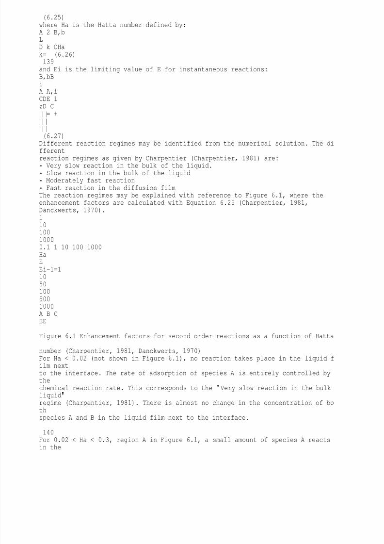
8/10/2019 Erasmus Mass 2004.PDF
http://slidepdf.com/reader/full/erasmus-mass-2004pdf 152/257
(6.25)where Ha is the Hatta number defined by:A 2 B,bLD k CHak= (6.26)139and Ei is the limiting value of E for instantaneous reactions:B,bBiA A,iCDE 1zD C
= + (6.27)Different reaction regimes may be identified from the numerical solution. The differentreaction regimes as given by Charpentier (Charpentier, 1981) are: Very slow reaction in the bulk of the liquid. Slow reaction in the bulk of the liquid Moderately fast reaction
Fast reaction in the diffusion filmThe reaction regimes may be explained with reference to Figure 6.1, where theenhancement factors are calculated with Equation 6.25 (Charpentier, 1981,Danckwerts, 1970).11010010000.1 1 10 100 1000HaEEi-1=110
501005001000A B CEE Figure 6.1 Enhancement factors for second order reactions as a function of Hatta number (Charpentier, 1981, Danckwerts, 1970)For Ha < 0.02 (not shown in Figure 6.1), no reaction takes place in the liquid film nextto the interface. The rate of adsorption of species A is entirely controlled by
thechemical reaction rate. This corresponds to the Very slow reaction in the bulkliquid
regime (Charpentier, 1981). There is almost no change in the concentration of bothspecies A and B in the liquid film next to the interface.
140For 0.02 < Ha < 0.3, region A in Figure 6.1, a small amount of species A reactsin the
8/10/2019 Erasmus Mass 2004.PDF
http://slidepdf.com/reader/full/erasmus-mass-2004pdf 153/257
diffusion film. The reaction takes place in the bulk of the liquid phase. Thereis aslight change in the concentration of species A across the liquid film next to theinterface. This regime is termed the Slow reaction in the liquid phase .
For 0.3 < Ha < 3.0, region B in Figure 6.1, a substantial amount of component Areacts in the liquid film. The concentration of component A is almost zero in the bulkof the liquid phase. This is the
Moderately fast
reaction regime.
For Ha > 3.0 the entire reaction takes place in the liquid film next to the interface.This corresponds to region C in Figure 6.1 and is termed the
fast reaction
regime.Two situations may now arise:
For 3 < Ha < Ei/2, the concentration of component B is much higher in the bulk of theliquid phase than the concentration of species A at the liquid interface. Theenhancement factor (E) lies close to the limiting diagonal line in Figure 6.1 (E » Ha).The kinetics of the reaction becomes pseudo first order with the reaction rateconstant changing to:
1 2 B,bk k C= (6.28)The diffusion rate of component B is sufficiently fast to prevent the reaction fromcausing significant depletion of component B at the interface. The concentration ofspecies B at the interface is almost the same as in the bulk of the liquid phase. Theabsorption rate then follow fast psuedo-first-order kinetics. The liquid side masstransfer coefficient becomes irrelevant and the average absorption rate may becalculated from:A A A,i A 2 B,bn N a aC D k C= = (6.29)This reaction regime forms the basis for measuring the interfacial area directly
fromthe rate of absorption. The specific absorption rate should however be known.
For Ha > 10Ei, the limiting value of E = Ei is reached (horizontal lines in region C inFigure 6.1). This situation arises when the concentration of reactant B is lessthan thesolubility of the gas or the mass transfer rate of reactant B from the bulk of the liquidto the interface is low and the dissolved gas reacts instantaneously with componentB. A reaction plane exists beneath the interface where the concentration of both
species is zero. The rate of the reaction is completely determined by the rate at141which the components diffuse towards the reaction plane. This reaction regime formsthe basis for measuring either kGa or kLa.
The above results for a second order reaction may be generalized for an m,nth orderirreversible reaction (rA=km,nCAmCBn). The enhancement factor may be approximate

8/10/2019 Erasmus Mass 2004.PDF
http://slidepdf.com/reader/full/erasmus-mass-2004pdf 154/257
dby (Hikita and Asai, 1964, Charpentier, 1981, Danckwerts, 1970):( ) ( )( ) ( ){ }n 2i in 2i iHa E E E 1Etanh Ha E E E 1
- -

8/10/2019 Erasmus Mass 2004.PDF
http://slidepdf.com/reader/full/erasmus-mass-2004pdf 155/257
= - -

8/10/2019 Erasmus Mass 2004.PDF
http://slidepdf.com/reader/full/erasmus-mass-2004pdf 156/257
(6.30)with the Hatta number defined as:0.5m 1 nm,n A A,i B,bL1 2Ha k D C Ck m 1- =
+
8/10/2019 Erasmus Mass 2004.PDF
http://slidepdf.com/reader/full/erasmus-mass-2004pdf 157/257
(6.31)and the enhancement factor for instantaneous reaction is the same as for secondorder reaction kinetics (Equation 6.27). If the reaction is fast and the concentration ofreagent B does not change significantly through the film, the reaction is pseudo mthorder with the rate constant given by:nm m,n B,bk k C= (6.32)The condition that has to be satisfied for a pseudo mth order reaction is 1 << Ha <<Ei. The average rate of absorption is then independent of kL and given by:0.5m 1 nA A m,n A A,i B,b2n N a a k D C Cm 1+ = = + (6.33)When determining the reaction kinetics in the fast pseudo mth order regime, it is oftennecessary to dilute the soluble gas with an insoluble gas in order to satisfy theconstraint on the Hatta number for the psuedo mth order regime (1 << Ha << Ei)(Charpentier, 1981, Danckwerts, 1970). Failure to do so will force the reactionintothe instantaneous reaction regime with depletion of the reactant B in the film n
ext tothe interface. When diluting the soluble gas, gas side resistance to mass transfermay arise. For a pseudo mth order reaction in the liquid phase, the absorption rate isthen given by (Charpentier, 1981):A A0.5Gm 1 nm,n A A,i B,bpn N a1 Hk a 2a k D C Cm 1 +
= =+
+ (6.34)where kG is the gas phase mass transfer coefficient, p the partial pressure of thesoluble gas in the bulk gas phase and H the Henry
s law constant.142
In order to determine the interfacial area with the chemical technique, it is importantthat the chosen gas-liquid reaction system fall into the rapid pseudo mth order
reaction regime. In order to determine the reaction kinetics for a given gas-liquidreaction system, knowledge of some physicochemical parameters need to beobtained. These include the kinetics of the reaction, the diffusivities of the soluble gasand the reactant in the liquid phase and the solubility of the gas in the liquid. Theseparameters are usually not determined separately but combined into the terms(Charpentier, 1981, Danckwerts, 1970):A,i AC D and

8/10/2019 Erasmus Mass 2004.PDF
http://slidepdf.com/reader/full/erasmus-mass-2004pdf 158/257
0.5m 1 nm,n A A,i B,b2 k D C Cm 1+ + (6.35)For rapid pseudo first order reactions, it is possible to determine the reaction rateconstant and the product of the solubility and the root of the diffusivity (thefirst termin Equation 6.35) from experimental absorption data. A so-called
Danckwerts plot isused (Danckwerts, 1970). For a reaction in the pseudo mth order regime, it is notpossible to determine these parameters separately from experimental absorptiondata. A neutral gas that have the same properties as the solute gas but that donotreact with the reagent have to be used to determine the property CA,i(DA)0.5. Whendetermining interfacial area in a gas-liquid contactor, it is not necessary to determinethe reaction kinetics and the physicochemical properties separately (Danckwerts, 1970, Charpentier, 1981). The specific absorption rate may be determined in alaboratory apparatus with a known interfacial area. The rapid pseudo mth order
reaction regime may be tested for by varying the contact time. If the absorption rateis independent of contact time, the reaction is suitable. If the solute gas is diluted witha non-absorbing carrier gas, gas phase resistance may arise. Steps may be takentoeliminate this resistance or it may be taken into account in the calculations. It ispreferable to eliminate gas phase resistance all together and determine the interfacialarea separately from kG.6.3.2 Laboratory apparatus for determining absorption ratesVarious laboratory apparatus are used to determine absorption rates in gas-liqui
dreactions. The essential features of such an apparatus are the interfacial areafor gasliquid contact and the contact time. There are a number of apparatus commonlyused. These include (Danckwerts, 1970) the rotating drum absorber, the movingband absorber, the wetted-wall column, the laminar jet, the string of disks andthestirred vessel. The gas-liquid contact time may be varied over a wide range by using143a combination of these absorbers for a given gas-liquid reaction. In this studyawetted wall column absorber is used. The contact times obtained with a wetted wa
llcolumn fall into the range of 0.1-2.0 seconds. This is close to the middle of the rangeobtained with the various devices. The choice of the wetted-wall column is alsoinpart due to previous experience and existing laboratory equipment (Erasmus andNieuwoudt, 2001). A detailed description of the column is given in the experimentalsection. The contact (or exposure) time of a liquid surface element to the gas phase
8/10/2019 Erasmus Mass 2004.PDF
http://slidepdf.com/reader/full/erasmus-mass-2004pdf 159/257
is calculated from classical laminar falling film theory (Danckwerts, 1970): m p= = r 2 31 3Li L3h 2h dtu 3 g V (6.36)where h is the height of the column, d the diameter of the column and VL thevolumetric liquid flow rate.Reaction mechanism between monoethanolamine (MEA) and CO2The stoichiometric reaction between carbon dioxide and monoethanolamine inaqueous solution may be expressed as (Danckwerts, 1979, Sada et al., 1985):2 2 2 3CO 2RNH RNHCO RNH- ++ fi + (6.37)where R represents HO-CH2-CH2-. The reaction is first order with respect to both carbon dioxide and monoethanolamine and overall second order (Danckwerts, 1979,Sada et al., 1985, Alvarez-Fuster et al., 1980). The proposed reaction mechanism involves two steps (Danckwerts, 1979). In the first step a
zwitterion
is formed:-+fi+ COORNHRNHCO222 (6.38)This is followed by the removal of a proton by a base B:
2RNH COO B RNH COO BH+ - + - ++ fi + (6.39)In aqueous medium the base may be H2O, OH- or the amine itself. The second stepis rate determining (Danckwerts, 1979). When the reaction takes place in analcoholic medium, the deprotonation of the zwitterion is depressed. The rate of thedeprotonation step (Equation 6.39) decreases relative to the rate of the reverse reaction (equation 6.38) (Versteeg and Van Swaaij, 1988). The alcohol solvent is notable to produce the zwitterion in complete ionic form and it is less stable. The overallreaction order then increases from 2 up to 3 (Versteeg and Van Swaaij, 1988). With a
steady state approximation of the
zwitterion
, the rate of the reaction may beexpressed as (Sada et al., 1985):144A B21 1 3 BC Crk1k k k C=+ (6.40)where B represents the amine and A carbon dioxide.
In this work the absorption rates were measured and used as is to determine theinterfacial area in structured packing by the method discussed in the precedingsection as recommended by Danckwerts (Danckwerts, 1970) and Charpentier(Charpentier, 1981). The rate constants were therefore not determined.6.4 Experimental6.4.1 Experimental setupWetted-wall columnThe wetted-wall column was constructed using the guidelines as suggested byRoberts and Danckwerts (Roberts and Danckwerts, 1962). The final design reflecte
8/10/2019 Erasmus Mass 2004.PDF
http://slidepdf.com/reader/full/erasmus-mass-2004pdf 160/257
dideas obtained from the designs of Roberts and Danckwerts (Roberts andDanckwerts, 1962) and Davies et al. (Davies et al., 1967). The wetted-wall column isshown in Figure 6.2. The column is made from stainless steel pipe with an outsidediameter of 25.1mm. The length of the column could be varied between 60mm and120mm by extending or collapsing it into the outlet section. The liquid is distributedaround the circumference of the tube by a special cap. The cap fits tightly over thetop 10mm of the wetted-wall column. This is followed by a 5 mm section that ismachined to a diameter of 28mm. The liquid enters this section through 12 evenly spaced holes around the circumference of the wetted wall column. This is followed bya section in the cap that has an inside diameter of 25.8mm, thus forming an annulargap of 0.35mm for the liquid to pass through. After passing through this annular passage (length approximately 15mm), the liquid finally free falls down the outside ofthe tube where contact with the gas phase is made. At the bottom of the column the
liquid exits through a special receiver (also called an exit collar (Roberts and Danckwerts, 1962)) that channels the liquid into 3 grooves (width 3mm) and finallyinto the exit annular passage formed between the bottom part of the wetted-wallcolumn and the base section. The base section screws into a stainless steel flange.The column is enclosed by a special glass QVF 3" pipe section bolted onto theflange. The flange is equipped with the gas inlet and gas outlet pipes and a drainpipein case of spillage. It is also equipped with three holes for threaded rod thatis used to145
level the column with the horizontal axis. The exit collar is included in the designbecause it prevents a stagnant film from developing at the bottom of the column(Roberts and Danckwerts, 1962). This stagnant film reduces the absorption rate inthis part of the column. Roberts and Danckwerts (Roberts and Danckwerts, 1962)found that using an exit collar could reduce this error. The stagnant film is thenconfined to the exit grooves of the collar. The liquid surface area in the grooves issmall compared to the rest of the wetted-wall column and may safely be ignored.
Figure 6.3 shows a flow diagram of the experimental setup. The whole wetted-wall
column assembly is submerged into a thermostat controlled water bath to ensureisothermal operation. The air is routed through a coil submerged in the water bathand the flow rate is controlled by a regulating valve. The flow rate is measured with asoap bubble meter that is also submerged into the water bath. It is then saturatedwith the solvent and mixed with carbon dioxide. The carbon dioxide flow rate iscontrolled through a regulating valve. The air/carbon dioxide mixture may either

8/10/2019 Erasmus Mass 2004.PDF
http://slidepdf.com/reader/full/erasmus-mass-2004pdf 161/257
bepassed through the wetted wall column and then to the carbon dioxide analyser, or itmay bypass the column and flow directly to the carbon dioxide analyser. The desiredcarbon dioxide concentration is obtained by bypassing the column and regulatingtheinlet pressure of the carbon dioxide until the desired concentration is obtained. Careis taken to ensure the same pressure drop through the system when the gas mixtureis routed through the column assembly or when bypassing it and flowing directlytothe carbon dioxide analyser. This is done to ensure a constant air and carbon dioxideflow rate. The air/carbon dioxide/solvent mixture passes through a cold trap tocondense as much of the solvent as possible before entering the analyser. The liquidis fed from a container elevated above the experimental setup to obtain gravityflowthrough the system. The flow rate is measured with a rotameter and controlled with aneedle valve. It passes through a coil submerged in the water bath before entering
the base of the wetted wall column. After exiting from the base section it flows over aconstant height overflow that is used to control the liquid level in the base section justunderneath the exit collar . The constant height overflow may be bypassed byopening a drain valve to drain the liquid in the base section. The height of the columnmay be varied by disconnecting the liquid feed line at the base and sliding thecolumn up or down through a tube fitting at the bottom of the base section. Allthematerials in contact with the liquid are either stainless steel or PTFE for corrosionresistance. PTFE ferrules are used at the base of the column to facilitate repea
tedlengthening and shortening of the column.1463" QVF Flange6 x M8 boltsDistributor cap3" QVF Pipe (modified)Gas inlet Gas outletLiquid inletLiquid outletBase sectionExit collarViton gasket
Venting screw25.1mm OD pipe12.7mm OD pipeBase flange Figure 6.2 Wetted-wall column 147AIRCO2Feedtank

8/10/2019 Erasmus Mass 2004.PDF
http://slidepdf.com/reader/full/erasmus-mass-2004pdf 162/257
PumpCO2 analyserEffluent tankSaturatorBubblemeterCold trapFlow regulatingvalvesThermostat controlled waterbathWetted-wall assemblyRotameterTITIVent Figure 6.3 Wetted-wall flow diagram 148Pilot plantThe pilot plant used in determining the effective surface area is to a large extent thesame as described in Chapter 4 and is shown in Figure 6.4. The column contains twopacked beds with a chimney tray between them. The desired airflow rate is obtain
edby throttling the intake to a centrifugal blower. The flow rate is measured with asquare-edged orifice plate. Carbon dioxide is mixed with the incoming air before entering the bottom packed bed. Liquid carbon dioxide is drawn from a cylinder witha dip tube. It is heated up to approximately 70oC before evaporating in the regulatorthat also controls the flow rate. In the lower packed bed the air is saturated with thesolvent. The solvent is circulated in a closed loop and replenished from time to time.
The temperature of the air after the saturation bed is controlled with the temperatureof the recirculating solvent. The solvent is heated with an electric heater. The air/carbon dioxide mixture enters the second packed bed through a chimney tray.The absorption of CO2 into the monethanolamine/alcohol solution takes place in thisbed. The liquid solution is pumped from a storage vessel through a rotameter and aheat exchanger to the top of the column. It is distributed evenly over the packed bedwith the distributor described and shown in Chapter 4. Liquid is drawn from thechimney tray through a constant height overflow. The constant height overflow ma
yalso be changed to operate as a liquid siphon draw. This is done at high liquidflowrates in order to prevent the chimney tray from overflowing. The loaded liquid thenflows under gravity to a storage vessel. The temperature of the air/carbon dioxidemixture and the MEA/alcohol mixture is measured on entering and on exiting theabsorption section. Gas sampling points are provided before and after the absorption

8/10/2019 Erasmus Mass 2004.PDF
http://slidepdf.com/reader/full/erasmus-mass-2004pdf 163/257
section. The gas sample stream flows through a cold trap to condense as much ofthe solvent possible before entering the CO2 analyser. The air/carbon dioxide/solventmixture from the top of the column is vented to the outside of the building.
The liquid from the absorption column is regenerated and recycled. This operation isperformed in a glass distillation column with a diameter of 200mm that is operated asa reboiled stripper. The column contains four beds of structured packing (Flexipac250Y HC) with the feed entering at the top. All the overhead vapour is condensed and returned back to the top of the column. Regenerated liquid is drawn from the reboiler and flows through a cooler under a nitrogen blanket to a storage vessel.Because of the low cooling capacity of the bottom product cooler, the wholeabsorption/regeneration cycle has to be performed in batch cycles.
149N2Solventvessel
MPIDPPump Pump Blower CO2ElectricheaterStoragevesselMass flowmeterSolventsaturationbed
CO2absorption bedVentStoragevesselTITITITITITITI
Cold trapCO2analyser Figure 6.4 PFD of pilot plant absorption column1506.4.2 Experimental procedureWetted-wall columnBefore doing absorption experiments in the wetted wall column reactor, a residence
8/10/2019 Erasmus Mass 2004.PDF
http://slidepdf.com/reader/full/erasmus-mass-2004pdf 164/257
time distribution experiment was performed. The RTD curve obtained correspondedto that of a CSTR and the gas phase could thus be assumed to be well mixed. Theconcentration of carbon dioxide in the exit gas stream is therefore equal to the bulkconcentration of carbon dioxide in the reactor.
Before the start of an experiment, the wetted wall column reactor was flushed with airat the desired flow rate. The bulb of the soap bubble meter was then removed and amanometer was used to measure the pressure at the base of the soap bubble meter. The wetted-wall reactor was then bypassed and the balancing valve on the outletlineadjusted until the same pressure was measured at the base of the soap bubblemeter. The manometer was removed and replaced with the bulb with soap solution.Carbon dioxide was now added and the flow rate adjusted until the desiredconcentration in the exit stream was obtained. The airflow rate was now measured.The air/carbon dioxide mixture was then routed through the reactor. The airflowratewas again measured to make sure that it was the same as when bypassing thereactor. Sufficient time was allowed for the exit stream carbon dioxide concentration
to reach the inlet stream concentration. The liquid feed was introduced and adjustedto the desired flow rate. The outlet concentration of carbon dioxide was monitoreduntil a steady value was reached. The temperatures of the liquid feed and air/carbondioxide/solvent gas feed as well as the pressure inside the reactor were recordedtogether with the flow rates and carbon dioxide concentrations. The liquid feedmixture was made up before the start of a series of experiments. The loaded liquid was regenerated before being used again. This was achieved by distillation under a
slightly reduced pressure at total reflux for approximately half an hour. The mixturewas then left to cool under a nitrogen blanket. After sufficiently cooling down, theliquid was transferred to airtight bottles.
A problem encountered when using a wetted-wall column is the formation of ripplesin the bottom part of the column (Danckwerts, 1970, Roberts and Danckwerts, 1962).These ripples were found to enhance absorption rates of soluble gases into a fallingfilm (Emmert and Pigford, 1954, Stirba and Hurt, 1955). A common method to
eliminate these ripples is to add an amount of surface active agent to the feed(Danckwerts, 1970, Roberts and Danckwerts, 1962, Sada et al., 1985). Two151surfactants were tested in this study. The agent used by Sada et al. (Sada et al.,1985), Tween 80 (polyoxyethylene solbitan monoleate), was successful in eliminatingthe ripples. There were however some concerns when using this surfactant. Thequantity suggested by the authors had to be doubled in order to obtain a ripplefree
8/10/2019 Erasmus Mass 2004.PDF
http://slidepdf.com/reader/full/erasmus-mass-2004pdf 165/257
surface. This may give rise to a surface resistance that will influence the absorptionrate (Roberts and Danckwerts, 1962). When regenerating the CO2 loaded solution,the surfactant was found to be thermally labile. The common surfactant Triton 100was also used but did not suppress the formation of ripples. Another method toeliminate the ripples is to work with short column lengths. Because of the problemsencountered with the addition of a surfactant, only short column lengths were used inthis study (maximum length of 90mm).Pilot plantBefore doing absorption experiments on the structured packing, the packing wasthoroughly washed with an acetone/alcohol mixture to rid it of any dirt and oilused inthe manufacturing process. The liquid feed was made up beforehand and left under anitrogen blanket to prevent atmospheric carbon dioxide from being absorbed.
With the start of an experiment the blower was switched on and throttled until thedesired flow rate was obtained. Carbon dioxide was mixed with the air and the flowrate adjusted until the desired concentration was obtained. The use of the carbo
ndioxide analyser and the mass flow meter also enabled the accuracy of the orificeplate to be measured. The error in the flow rate measured with the orifice plate wascalculated to be less than 5%. The solvent was then introduced into the saturationbed and the temperature adjusted until the desired exit temperature of the air/carbondioxide/solvent mixture was obtained. This temperature could be controlled to be within 3oC of the liquid feed. The liquid feed was then introduced into the absorption
bed. The flow rates and temperatures of all the inlet and exit streams were noted, aswell as the pressure inside the column. The concentration carbon dioxide in theinletand outlet gas streams was then measured. The absorption rate was measured atdifferent liquid loads for the same gas load by altering the liquid feed rate. Theamount of liquid feed was sufficient for the absorption rate to be measured at fourdifferent liquid loads before regeneration. This corresponded to the total amount ofmeasurement at a specific gas flow rate. After regeneration the feed liquid wasleft to
cool down overnight under a nitrogen blanket.
152AnalysisThere are a few methods commonly used determine the loading of CO2 in amines inaqueous media (Shahi et al., 1994). In the volumetric method sulphuric acid is addedto a known amount of loaded sample and the amount of evolved CO2 is measured.With the wet chemistry method the CO2 in the sample is precipitated by adding aBaCl2 solution to the sample. The precipitate may then either be weighed or

8/10/2019 Erasmus Mass 2004.PDF
http://slidepdf.com/reader/full/erasmus-mass-2004pdf 166/257
dissolved in water and titrated against a standard acid solution. These methodswerehowever found to be tedious and not accurate when the CO2 loading is low (Shahietal., 1994). The extension of these methods to organic media is difficult. One of themain difficulties is the formation of two liquid phases when titrating against a standardacid or base. A GC technique was recently developed (Shahi et al., 1994) where theCO2 loading and concentration of amine could be determined simultaneously. Themethods uses a Tenax GC column with a TCD detector. The CO2/amine complex(also called a carbamic acid) is thermally unstable and decomposes in the injectorport (Alvarez-Fuster et al., 1981) (Shahi et al., 1994). The main difficulty iscalibrationfor CO2. The method was tested in this study, but no reproducible calibration resultscould be obtained to determine CO2 content. Because of the difficulty and inaccuracyof determining the CO2 content of the liquid phase, only the gas phase was analysedfor CO2 concentration. The GC technique was used to determine the CO2 content in
the feed samples qualitatively after regeneration. The regeneration column wasoperated in such a manner (low feed rate, high boil-up rate) that there was no CO2detectable in the GC chromatogram. The feed was kept in a closed container under anitrogen blanket to eliminate the possibility of absorbing atmospheric CO2. Theconcentration of the amine in the liquid phase was determined with the GCtechnique. For the wetted-wall experiments the concentration was determined byweighing the reagents.
The CO2 concentration in the gas phase was measured with an infrared carbondioxide analyser (Dräger Multiwarn Multi-Gas Monitor equipped with an infrared CO2
sensor).6.5 Results and discussionBoth n-propanol and n-butanol were identified as possible solvents. Problems were,however, encountered with the analysis of n-butanol liquid samples in the preliminarystages of the investigation. This was mainly due to immiscible phases forming whenusing titration with a standard acid to determine MEA content. No separation153between MEA and n-butanol could be obtained in the Tenax GC column. Separationbetween MEA and n-propanol could be obtained with this column and the use of n-butanol as solvent was subsequently abandoned in favour of n-propanol. The
physical properties for the system MEA/n-propanol are given in Appendix E. Thedensity and viscosity dependence was found to be the same as determined byAlvarez-Fuster et al. (Alvarez-Fuster et al., 1981) for the system MEA/ethanol.6.5.1 Experimental determined absorption ratesThe rate of absorption of CO2 into MEA with n-propanol as solvent was determined with the wetted-wall column reactor described in the previous section. When dilutingthe solute gas (CO2) with a carrier gas (air) as was done in this study, gas phase

8/10/2019 Erasmus Mass 2004.PDF
http://slidepdf.com/reader/full/erasmus-mass-2004pdf 167/257
resistance to mass transfer may arise. This resistance may be eliminated by workingat high gas flow rates with a subsequent small change in the inlet and outletconcentrations of CO2 (Danckwerts, 1970). There should however still be a largeenough difference between the inlet and outlet concentration to accurately determinethe amount absorbed in the liquid phase, since in this study the liquid phase was notanalysed for CO2 content. High absorption rates with a significant resistance in thegas phase were encountered at high concentrations of MEA (0.5-1.0 mol/dm3) andlarge CO2 partial pressures (2.0-5.0 kPa). The experimental setup could not beconverted to facilitate large enough airflow rates to eliminate gas phase resistance.The absorption rates were therefore determined at the highest MEA and CO2concentrations possible with the experimental setup without substantial gas phaseresistance. This corresponded to a maximum MEA concentration of 0.3 mol/dm3 anda maximum CO2 partial pressure of 1.2 kPa. The absorption rates were determinedat two temperatures, 288K and 303K. This was done because the pilot plantexperiments were performed at ambient conditions and the ambient temperaturevaried in this range. The contact time was varied by working with wetted-wall columnheights of 60 mm and 90 mm and using liquid flow rates of 1.0 cm3/s and 1.6 cm3/
s.For the reaction to be in the pseudo m-nth order regime, the absorption rate must beindependent of the contact time. Figure 6.5 show the specific absorption rate at different contact times for a MEA concentration of 0.3 mol/dm3 at a temperatureof288 K. The figure shows that the absorption rates are practically the same at differentcontact times. The marginally higher specific absorption rates at lower contacttimesare within the experimental error. These errors are mainly due to the resolution of the
infrared CO2 analyser (0.01 vol% CO2) and the adjustment of the column length(±1mm). Figure 6.6 show the specific absorption rates as a function of the CO2 partial154pressure at different MEA concentrations (T=288 K). The absorption rate increasesas the amine concentration increases.2.02.53.03.54.04.5
5.05.56.06.57.00.4 0.6 0.8 1.0 1.2PCO2 [kPa]NA

8/10/2019 Erasmus Mass 2004.PDF
http://slidepdf.com/reader/full/erasmus-mass-2004pdf 168/257
x 104 [mol/(m2.s)]tc = 0.55tc = 0.83tc = 1.1Contact time, [s]NA
x 104 [mol/(
m2.s)] Figure 6.5 Verification of pseudo m,nth order reaction. CMEA=0.3 mol/dm3,T=288K.Figure 6.7 show the specific absorption rates at 288 K and 303 K for a MEAconcentration of 0.2 mol/dm3. The absorption rate is higher at the lower temperature.At low CO2 partial pressures (<0.5 kPa) the absorption rate is almost the same a
t 288K and 303 K.
The experimental determined absorption rates were correlated with a power lawseries with amine concentration (CB) and CO2 partial pressure (PA) as variables: m nA A BN kP C= (6.41)Equations similar to that proposed by Sada et al. (Sada et al., 1985) (Equation6.40)and Alvarez-Fuster et al. (Alvarez-Fuster et al., 1980) for the reaction rate di
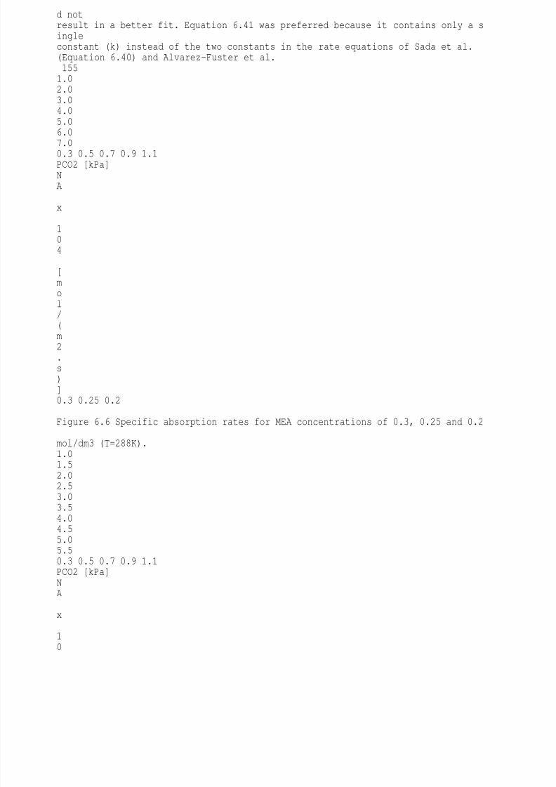
8/10/2019 Erasmus Mass 2004.PDF
http://slidepdf.com/reader/full/erasmus-mass-2004pdf 169/257
d notresult in a better fit. Equation 6.41 was preferred because it contains only a singleconstant (k) instead of the two constants in the rate equations of Sada et al.(Equation 6.40) and Alvarez-Fuster et al.1551.02.03.04.05.06.07.00.3 0.5 0.7 0.9 1.1PCO2 [kPa]NA x 104
[mol/(m2.s)]0.3 0.25 0.2
Figure 6.6 Specific absorption rates for MEA concentrations of 0.3, 0.25 and 0.2 mol/dm3 (T=288K).1.01.52.02.53.03.54.04.55.0
5.50.3 0.5 0.7 0.9 1.1PCO2 [kPa]NA x 10
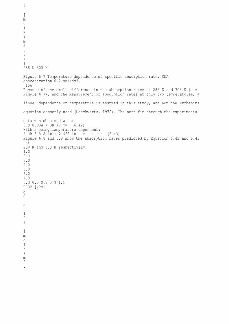
8/10/2019 Erasmus Mass 2004.PDF
http://slidepdf.com/reader/full/erasmus-mass-2004pdf 170/257
4 [mol/(m2.s)]288 K 303 K Figure 6.7 Temperature dependence of specific absorption rate. MEAconcentration 0.2 mol/dm3.156Because of the small difference in the absorption rates at 288 K and 303 K (seeFigure 6.7), and the measurement of absorption rates at only two temperatures, a linear dependence on temperature is assumed in this study, and not the Arrhenius
equation commonly used (Danckwerts, 1970). The best fit through the experimental data was obtained with:0.9 0.93A A BN kP C= (6.42)with k being temperature dependent:6 3k 3.818 10 T 2.985 10- -= - · + · (6.43)Figure 6.8 and 6.9 show the absorption rates predicted by Equation 6.42 and 6.43 at288 K and 303 K respectively.1.02.03.04.0
5.06.07.00.3 0.5 0.7 0.9 1.1PCO2 [kPa]NA x 104
[mol/(m2.
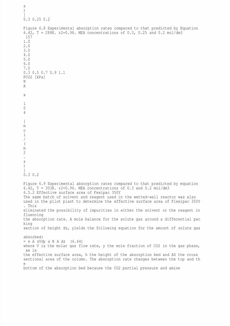
8/10/2019 Erasmus Mass 2004.PDF
http://slidepdf.com/reader/full/erasmus-mass-2004pdf 171/257
s)]0.3 0.25 0.2 Figure 6.8 Experimental absorption rates compared to that predicted by Equation6.42, T = 288K. r2=0.98. MEA concentrations of 0.3, 0.25 and 0.2 mol/dm31571.02.03.04.05.06.07.00.3 0.5 0.7 0.9 1.1PCO2 [kPa]NA x 10
4 [mol/(m2.s)
]0.3 0.2 Figure 6.9 Experimental absorption rates compared to that predicted by equation6.42, T = 303K. r2=0.96. MEA concentrations of 0.3 and 0.2 mol/dm36.5.2 Effective surface area of Fexipac 350YThe same batch of solvent and reagent used in the wetted-wall reactor was alsoused in the pilot plant to determine the effective surface area of Flexipac 350Y. Thiseliminated the possibility of impurities in either the solvent or the reagent influencingthe absorption rate. A mole balance for the solute gas around a differential packing
section of height dz, yields the following equation for the amount of solute gas absorbed:= e A sVdy a N A dz (6.44)where V is the molar gas flow rate, y the mole fraction of CO2 in the gas phase, ae isthe effective surface area, h the height of the absorption bed and AS the crosssectional area of the column. The absorption rate changes between the top and thebottom of the absorption bed because the CO2 partial pressure and amine
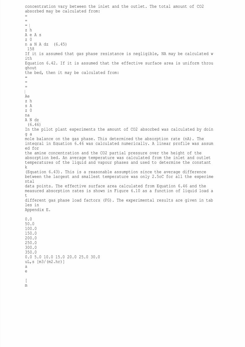
8/10/2019 Erasmus Mass 2004.PDF
http://slidepdf.com/reader/full/erasmus-mass-2004pdf 172/257
concentration vary between the inlet and the outlet. The total amount of CO2absorbed may be calculated from:=== z hA e A sz 0n a N A dz (6.45)158If it is assumed that gas phase resistance is negligible, NA may be calculated withEquation 6.42. If it is assumed that the effective surface area is uniform throughoutthe bed, then it may be calculated from:===
Aez hs Az 0na
A N dz (6.46)In the pilot plant experiments the amount of CO2 absorbed was calculated by doing amole balance on the gas phase. This determined the absorption rate (nA). Theintegral in Equation 6.46 was calculated numerically. A linear profile was assumed forthe amine concentration and the CO2 partial pressure over the height of theabsorption bed. An average temperature was calculated from the inlet and outlettemperatures of the liquid and vapour phases and used to determine the constantk(Equation 6.43). This is a reasonable assumption since the average differencebetween the largest and smallest temperature was only 2.5oC for all the experime
ntaldata points. The effective surface area calculated from Equation 6.46 and themeasured absorption rates is shown in Figure 6.10 as a function of liquid load atdifferent gas phase load factors (FG). The experimental results are given in tables inAppendix E.
0.050.0100.0150.0200.0
250.0300.0350.00.0 5.0 10.0 15.0 20.0 25.0 30.0uL,s [m3/(m2.hr)]ae [m

8/10/2019 Erasmus Mass 2004.PDF
http://slidepdf.com/reader/full/erasmus-mass-2004pdf 173/257

8/10/2019 Erasmus Mass 2004.PDF
http://slidepdf.com/reader/full/erasmus-mass-2004pdf 174/257
[m2/m3]1.1 1.5 2.0FG [(m/s)(kg/m3)0.5]+ confidence- confidenceae [m2/m3] Figure 6.11 Experimental data plotted with upper and lower confidence limits
The sensitivity of the effective surface shown in Figure 6.10 to the accuracy of theinfrared CO2 analyser was determined as follows. The resolution of the digital display160(0.01vol%) was added to or subtracted from the difference between the inlet andoutlet concentrations. This resulted in a difference in the calculated effective surfacearea of ±6% at the highest absorption rate and ±15% at the lowest absorption rate.The experimental error at the lowest absorption rate (uL,s 6.0 m3/(m2.hr)) istherefore in the order of 20% while at the highest liquid load it is in the order of 10%.These confidence limits are plotted with the data in Figure 6.11.
6.5.3 Comparison with existing correlationsThe experimentally determined effective interfacial area is compared with thatcalculated from the correlations and methods discussed in Section 6.2 in Figure6.12.0.050.0100.0150.0200.0250.0300.0350.0400.0
450.00.0 5.0 10.0 15.0 20.0 25.0 30.0uL,s [m3/(m2.hr)]ae [m2/
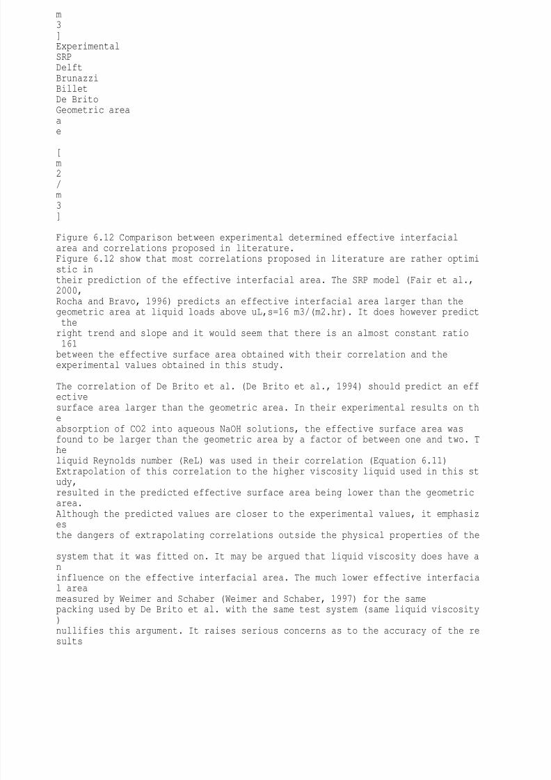
8/10/2019 Erasmus Mass 2004.PDF
http://slidepdf.com/reader/full/erasmus-mass-2004pdf 175/257
m3]ExperimentalSRPDelftBrunazziBilletDe BritoGeometric areaae [m2/m3] Figure 6.12 Comparison between experimental determined effective interfacialarea and correlations proposed in literature.Figure 6.12 show that most correlations proposed in literature are rather optimi
stic intheir prediction of the effective interfacial area. The SRP model (Fair et al.,2000,Rocha and Bravo, 1996) predicts an effective interfacial area larger than thegeometric area at liquid loads above uL,s=16 m3/(m2.hr). It does however predict theright trend and slope and it would seem that there is an almost constant ratio161between the effective surface area obtained with their correlation and theexperimental values obtained in this study.
The correlation of De Brito et al. (De Brito et al., 1994) should predict an effective
surface area larger than the geometric area. In their experimental results on theabsorption of CO2 into aqueous NaOH solutions, the effective surface area wasfound to be larger than the geometric area by a factor of between one and two. Theliquid Reynolds number (ReL) was used in their correlation (Equation 6.11)Extrapolation of this correlation to the higher viscosity liquid used in this study,resulted in the predicted effective surface area being lower than the geometricarea.Although the predicted values are closer to the experimental values, it emphasizesthe dangers of extrapolating correlations outside the physical properties of the
system that it was fitted on. It may be argued that liquid viscosity does have aninfluence on the effective interfacial area. The much lower effective interfacial areameasured by Weimer and Schaber (Weimer and Schaber, 1997) for the samepacking used by De Brito et al. with the same test system (same liquid viscosity)nullifies this argument. It raises serious concerns as to the accuracy of the results
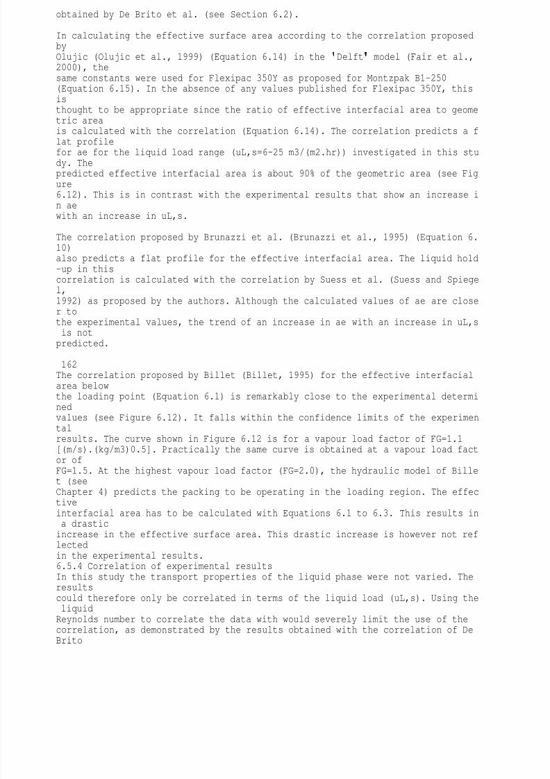
8/10/2019 Erasmus Mass 2004.PDF
http://slidepdf.com/reader/full/erasmus-mass-2004pdf 176/257
obtained by De Brito et al. (see Section 6.2).
In calculating the effective surface area according to the correlation proposedbyOlujic (Olujic et al., 1999) (Equation 6.14) in the Delft model (Fair et al.,2000), thesame constants were used for Flexipac 350Y as proposed for Montzpak B1-250(Equation 6.15). In the absence of any values published for Flexipac 350Y, thisisthought to be appropriate since the ratio of effective interfacial area to geometric areais calculated with the correlation (Equation 6.14). The correlation predicts a flat profilefor ae for the liquid load range (uL,s=6-25 m3/(m2.hr)) investigated in this study. Thepredicted effective interfacial area is about 90% of the geometric area (see Figure6.12). This is in contrast with the experimental results that show an increase in aewith an increase in uL,s.
The correlation proposed by Brunazzi et al. (Brunazzi et al., 1995) (Equation 6.10)also predicts a flat profile for the effective interfacial area. The liquid hold
-up in thiscorrelation is calculated with the correlation by Suess et al. (Suess and Spiegel,1992) as proposed by the authors. Although the calculated values of ae are closer tothe experimental values, the trend of an increase in ae with an increase in uL,s is notpredicted.
162The correlation proposed by Billet (Billet, 1995) for the effective interfacialarea belowthe loading point (Equation 6.1) is remarkably close to the experimental determi
nedvalues (see Figure 6.12). It falls within the confidence limits of the experimentalresults. The curve shown in Figure 6.12 is for a vapour load factor of FG=1.1[(m/s).(kg/m3)0.5]. Practically the same curve is obtained at a vapour load factor ofFG=1.5. At the highest vapour load factor (FG=2.0), the hydraulic model of Billet (seeChapter 4) predicts the packing to be operating in the loading region. The effectiveinterfacial area has to be calculated with Equations 6.1 to 6.3. This results in a drasticincrease in the effective surface area. This drastic increase is however not ref
lectedin the experimental results.6.5.4 Correlation of experimental resultsIn this study the transport properties of the liquid phase were not varied. Theresultscould therefore only be correlated in terms of the liquid load (uL,s). Using the liquidReynolds number to correlate the data with would severely limit the use of thecorrelation, as demonstrated by the results obtained with the correlation of DeBrito

8/10/2019 Erasmus Mass 2004.PDF
http://slidepdf.com/reader/full/erasmus-mass-2004pdf 177/257
et al. From the comparison of existing correlations with the experimental data,itwould seem that the correct trends are predicted by the SRP correlation and thecorrelation by Billet. The correlation by Billet is remarkably accurate in predicting theexperimental results. More experimental data on the effective surface area using thechemical method are however necessary in order to verify the dependency of theeffective surface area on the liquid transport properties as suggested by thecorrelation of Billet and the correlation in the SRP model.
Figure 6.10 shows the increase in effective surface area follows a logarithmic trendwith an increase in the liquid load. This is to be expected since at an almost zeroliquid load very little of the packing will be wetted. At high liquid loadings almost all ofthe geometric area of the packing will be wetted. All the geometric area will not beeffective for gas phase mass transfer. The effective surface area will therefore approach the geometric area asymptotically with an increase in the liquid load.Theratio of the effective surface area to the geometric surface area was therefore
correlated with the following logarithmic relationship:( )-= + · +3e L,spa 0.331 Ln u 1 10 2.29a (6.47)163where uL,s is the superficial liquid velocity with units [m3/(m2.s)]. This equation is validfor a superficial liquid load in the range 6.0 uL,s [m3/(m2.hr)] 25.0. The propertiesof the liquid phase are:m : 2.0·10-3 [Pa.s]r : 800 [kg/m3]
s : 23.5 [mN/m]The values obtained with this equation are compared with the experimental results inFigure 6.13.0.00.10.20.30.40.50.60.70.8
0.91.00.0 5.0 10.0 15.0 20.0 25.0 30.0uL,s [m3/(m2.hr)]ae/ap
8/10/2019 Erasmus Mass 2004.PDF
http://slidepdf.com/reader/full/erasmus-mass-2004pdf 178/257
experimentalEquation 6.47 Figure 6.13 Comparison of experimental results with that predicted by Equation6.47At liquid loads in excess of uL,s = 30 [m3/(m2.hr)], Equation 6.47 predicts a gradualincrease in ae up to about uL,s = 80 [m3/(m2.hr)] where the effective surface is equal tothe geometric area (ae/ap=1). Equation 6.47 would be conservative in estimatingtheeffective surface area at liquid loads higher than uL,s = 30 [m3/(m2.hr)] coupled withvapour load factors higher than FG = 2.0 [(m/s).(kg/m3)0.5].1646.6 ConclusionsThe following conclusions may be drawn from the investigation of the effectivesurface area of structured packing and more specifically Flexipac 350Y: A literature review revealed conflicting results obtained in the measurement ofeffective interfacial area in structured packing. The absorption of CO2 into monoethanolamine with n-propanol as solvent wasidentified as an alternative organic system for determining effective interfacialarea in structured packing.
The measurement of specific absorption rates in a wetted-wall reactor showedthat the kinetics of the reaction between CO2 and MEA with n-propanol assolvent falls into the rapid pseudo m,nth order reaction regime. The specific absorption rate of CO2 (0.45 PA [kPa] 1.1) into MEA with n-propanol as solvent (0.2 CB [mol/dm3] 0.3) is predicted by:0.9 0.93A A BN kP C=with k being temperature dependent (288 T [K] 303):6 3k 3.818 10 T 2.985 10- -= - · + · Current correlations available in literature tend to over predict the effectiveinterfacial area of Flexipac 350Y. The correlation proposed by Billet (Billet, 1995)is an exception and predicts the effective surface area of Flexipac accuratelybelow the loading point.
The experimental determined effective surface area of Flexipac 350Y shows alogarithmic trend with increasing liquid load. The experimental results werecorrelated with:( )-= + · +3e L,spa 0.331 Ln u 1 10 2.29auL,s is the superficial liquid velocity with units [m3/(m2.s)]. This equation is valid for a superficial liquid load in the range 6.0 uL,s[m3/(m2.hr)] 25.0. The liquid phase had the following properties:m : 2.0·10-3 [Pa.s]r : 800 [kg/m3]s : 23.5 [mN/m]
The effective surface area was found to be independent of the vapour load factor in the range 1.1 FG [(m/s).(kg/m3)0.5] 2.0 for the experimental liquid loadsinvestigated.1656.7 Nomenclaturea Area [m2]ae Effective surface area [m2/m3]ap Geometric area of packing [m2/m3]As cross sectional area of column [m2]
8/10/2019 Erasmus Mass 2004.PDF
http://slidepdf.com/reader/full/erasmus-mass-2004pdf 179/257
C Concentration [mol/m3]D Diffusion coefficient [m2/s]dh Hydraulic diameter [m]dx Differential distance in x-coordinate direction [m]E Enhancement factor due to chemical reaction [-]Ei Enhancement factor due to instantaneous chemical reaction [-]FG Vapour phase capacity factor [(m/s)(kg/m3)0.5]Fr Froude number [-]FSE Factor accounting for surface treatment of packing [-]g Acceleration due to gravity [m/s2]h height of wetted-wall column [m]H Henry
s law constant [Pa.m3/mol]Ha Hatta number [-]ht Total liquid holdup [m3/m3]kG,kL Mass transfer coefficients [m/s]k Reaction rate constant [dependant on order of reaction]Ma Marangoni number [-]n Molar flux [mol/s]N Specific molar flux [mol/(m2.s)]P Pressure [Pa]Re Reynolds number [-]S Channel side dimension [m]T Temperature [K]t time [s]
u Velocity [m/s]V Volumetric flow rate [m3/s] or molar flow rate [mol/s]We Weber number [-]x Mole fraction [-]z Stoichiometric relationship [-]166Greekp = 3.14159¼q Corrugation angle [o]b Discount factor for incomplete wetting [-]m Dynamic viscosity [Pa.s]W Fraction of packing area occupied by holes [-]s Surface tension [N/m]
d Film thickness [m]e Void fraction [-]g Contact angle between solid and liquid [o]r Density [kg/m3]Subscriptslp Refers to loading pointfp Refers to flood pointe EffectiveG Refers to vapour phase propertyL Refers to liquid phase propertys SuperficialW Refers to property of waterneg Refers to surface negative systems
A Refers to component AB Refers to component Bi Refers to interface between vapour/liquid phasesb Refers to bulk phase
1677 BINARY DISTILLATION IN STRUCTURED PACKING7.1 IntroductionThere is a large amount of data on the efficiency of structured packing publishe
8/10/2019 Erasmus Mass 2004.PDF
http://slidepdf.com/reader/full/erasmus-mass-2004pdf 180/257
d inthe brochures of different packing vendors. These data are however only available inthe form of efficiency and pressure drop curves and are therefore of limited use whendeveloping mass transfer correlations and pressure drop models. In this study, a large databank of binary distillation data was developed. This was done in order totest the correlations for the vapour phase mass transfer coefficient and effectivesurface area developed in Chapters 5 and 6 and to compare them with existingmodels in the literature for efficiency and pressure drop. The increase in capacityoffered by the new range of high capacity packing was also investigated. Thischapter is therefore divided into two parts. The first deals with the characterization ofthe different types of packing and the comparison between the normal capacitypacking and the new generation of high capacity packing. In the second part theefficiency and pressure drop are compared to those predicted by the different modelsin literature and the correlations developed in this study.7.2 Characterization of structured packingIt is common practice to state the efficiency of structured packing in terms of
theHETP or height equivalent to a theoretical plate. In order to determine the HETP of apacking, a standard binary test mixture is used for which the VLE is accuratelyknown. The HETP is then determined from the total packing height and the numberof equilibrium stages necessary to achieve the experimental determined separation.An equilibrium model simulator was developed in this study to determine the numberof equilibrium stages. The test mixture chlorobenzene/ethylbenzene was used. Itis astandard test mixture recommended by the IChemE (Onken and Arlt, 1990) forcolumns operating under atmospheric and vacuum conditions and with a number of
theoretical stages of between 10 and 30. One of the goals of this study, as setout inChapter 1, was to quantify the increase in capacity offered by the high capacity structured packing over the older third generation structured packing. Flexipac350YHC is compared with Flexipac 350Y.1687.3 Predicting separation efficiency and pressure drop forFlexipac 350YThe large amount of data generated enabled thorough testing of existing efficiencyand pressure drop models and the new correlations for vapour phase mass transfer
and effective surface area developed in this study. The SRP, Delft and Billet modelswere identified to be suitable for determining the capacity and efficiency of Flexipac350Y. The pressure drop and holdup equations used in the different models arediscussed in detail in Chapter 4. The mass transfer correlations and effective surfacearea equations are given in Chapters 5 and 6. A short summary of the mass transfer
8/10/2019 Erasmus Mass 2004.PDF
http://slidepdf.com/reader/full/erasmus-mass-2004pdf 181/257
correlations and effective surface area equations are given in the followingparagraphs for each of these models. A more detailed summary of each model isgiven in Appendix B and the various chapters dealing with the specific subject.Fordefinitions of the various dimensionless numbers, Appendix B should be consulted.
The SRP model use a wetted-wall type correlation for the vapour phase masstransfer coefficient:( ) 0.8G,e L,e G 0.33G GGu u SSh 0.054 Sc + r =
m (7.1)The liquid phase mass transfer coefficient is calculated according to the penetrationtheory of Higbie with the surface exposure time calculated as the time it takesfor aliquid element to flow a distance equal to the side dimension of the packing. Adiscount factor (CE) is incorporated to account for parts of the bed that do not encourage rapid surface renewal:L L,eL
E hGD uk 2C d= p (7.2)The effective surface area is calculated with a correlation adapted from Shi and Mersmann (Shi and Mersmann, 1985) for rivulet width on an inclined plate (asdiscussed in Chapter 6):( )( )( )= e - g q0.15 0.359L,s L,seSE 0.30.2 0.6p L,s
29.12 We Fr Sa Fa Re 1 0.93cos sin (7.3)The vapour phase mass transfer coefficient in the Delft model is calculated from laminar and turbulent contributions according to2 2G G,lam G,turbk k k= + (7.4)169with the laminar contribution calculated with:= G,lam hG 1/ 3 hGG G,rG G,pek d d0.664Sc ReD (7.5)The turbulent contribution is calculated from:
( )x j
= +
x j + -
8/10/2019 Erasmus Mass 2004.PDF
http://slidepdf.com/reader/full/erasmus-mass-2004pdf 182/257
GL 2 / 3G,r GG,turb hG hGG G,pe2 / 3GLGRe Sck d d81D1 12.7 Sc 18 (7.6)The gas-liquid interaction coefficient (xGL) follows from their hydraulic model(seeChapter 4). The liquid phase mass transfer coefficient is calculated with the sameequation proposed by the SRP model but with a characteristic length equal to the hydraulic diameter of the vapour phase:L L,eLhGD uk 20.9d= p (7.7)The effective surface area is calculated from:( )( )
- W= + e pBL,s1a aA1u (7.8)The vapour phase mass transfer coefficient in the Billet model is calculated fro
m:=e -131.5p e34G e G G G,s Gph ta a1k a C D Re Scad h (7.9)Different correlations are used for the liquid phase mass transfer coefficient belowand above the loading point. Below the loading point kL is calculated from:
=
11 12 eL2 2L e L p L,eh paDk a 12 C a ud a (7.10)and above the loading point with:
=

8/10/2019 Erasmus Mass 2004.PDF
http://slidepdf.com/reader/full/erasmus-mass-2004pdf 183/257
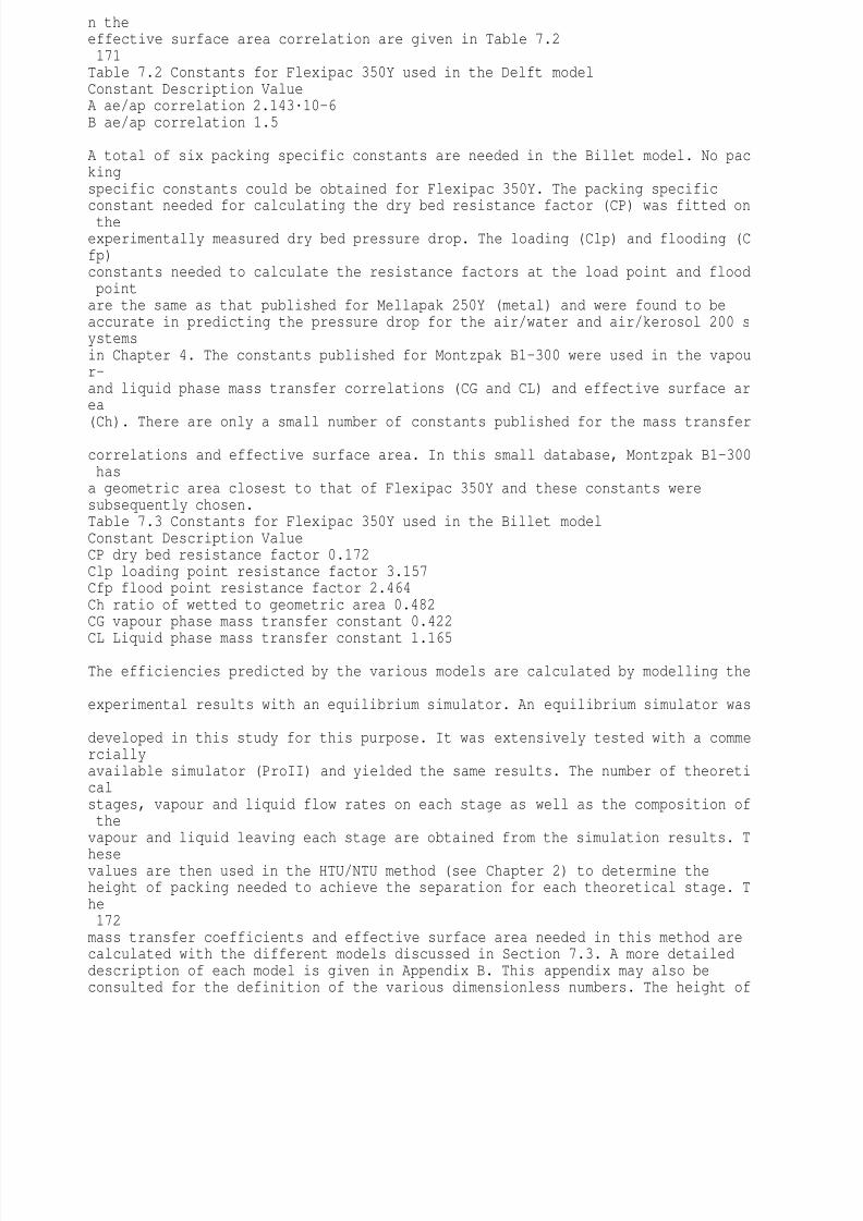
8/10/2019 Erasmus Mass 2004.PDF
http://slidepdf.com/reader/full/erasmus-mass-2004pdf 184/257
n theeffective surface area correlation are given in Table 7.2171Table 7.2 Constants for Flexipac 350Y used in the Delft modelConstant Description ValueA ae/ap correlation 2.143·10-6B ae/ap correlation 1.5
A total of six packing specific constants are needed in the Billet model. No packingspecific constants could be obtained for Flexipac 350Y. The packing specificconstant needed for calculating the dry bed resistance factor (CP) was fitted on theexperimentally measured dry bed pressure drop. The loading (Clp) and flooding (Cfp)constants needed to calculate the resistance factors at the load point and flood pointare the same as that published for Mellapak 250Y (metal) and were found to beaccurate in predicting the pressure drop for the air/water and air/kerosol 200 systemsin Chapter 4. The constants published for Montzpak B1-300 were used in the vapour-and liquid phase mass transfer correlations (CG and CL) and effective surface area
(Ch). There are only a small number of constants published for the mass transfer correlations and effective surface area. In this small database, Montzpak B1-300 hasa geometric area closest to that of Flexipac 350Y and these constants weresubsequently chosen.Table 7.3 Constants for Flexipac 350Y used in the Billet modelConstant Description ValueCP dry bed resistance factor 0.172Clp loading point resistance factor 3.157Cfp flood point resistance factor 2.464Ch ratio of wetted to geometric area 0.482CG vapour phase mass transfer constant 0.422
CL Liquid phase mass transfer constant 1.165
The efficiencies predicted by the various models are calculated by modelling the experimental results with an equilibrium simulator. An equilibrium simulator was developed in this study for this purpose. It was extensively tested with a commerciallyavailable simulator (ProII) and yielded the same results. The number of theoreticalstages, vapour and liquid flow rates on each stage as well as the composition of thevapour and liquid leaving each stage are obtained from the simulation results. T
hesevalues are then used in the HTU/NTU method (see Chapter 2) to determine theheight of packing needed to achieve the separation for each theoretical stage. The172mass transfer coefficients and effective surface area needed in this method arecalculated with the different models discussed in Section 7.3. A more detaileddescription of each model is given in Appendix B. This appendix may also beconsulted for the definition of the various dimensionless numbers. The height of

8/10/2019 Erasmus Mass 2004.PDF
http://slidepdf.com/reader/full/erasmus-mass-2004pdf 185/257
packing for each theoretical stage is also calculated with the correlations developedin this study. This is done by assuming no resistance to mass transfer in the liquidphase and using Equation 5.48 for the vapour phase mass transfer coefficient and Equation 6.47 for the effective surface area. The effective vapour phase velocity(uG,e) needed to determine the effective vapour phase Reynolds number (ReG,e) in Equation 5.48 is calculated from:( )G,sG,etuu1 h sin= e - q (7.13)The liquid holdup (ht) is calculated with the equation proposed in the Delft model(Equation 4.62 and 4.63). The effective vapour phase Reynolds number in Equation 5.48 is calculated with:r=m
G G,e hGG,eGu dRe (7.14)The hydraulic diameter for the vapour phase is the same as defined in Chapter 5: =hG Bhd S (7.15)The total height of packing is calculated by summing the heights of packing (orHETP) calculated for each stage. An average HETP is calculated by dividing the totalheight by the number of stages. Linear interpolation is used to calculate fractions of atheoretical stage in order to achieve the experimentally determined separation.
7.4 Experimental7.4.1 SetupThe column used in this study was specifically set up to operate under conditions oftotal reflux and is shown in Figure 7.1. The column is constructed from four 200 mmID glass segments. The height of each segment is 1m and accommodates 3structured packing elements. The column therefore contained 4 packed beds with theheight of packing in each bed equal to the height of 3 packing elements. Wheninstalling the elements in the column segments, each element was rotated 90o with
respect to the previous one. At the bottom of the column the first packing elementwas installed with the channels aligned with the reboiler return line. This wasdone to173eliminate any possible vapour phase maldistribution. A modification had to be madeto the standard column segments commercially available. They are supplied withsupport rings about 100mm from the bottom. These support rings are used to holda

8/10/2019 Erasmus Mass 2004.PDF
http://slidepdf.com/reader/full/erasmus-mass-2004pdf 186/257
support grid in place when packing the column with random packing. At thesesupport rings the diameter of the column is reduced from 200mm to 160mm. It wasfound that these support rings drastically reduced the capacity of the column andthey were subsequently removed. The condenser is located at the top of the columnand all the distillate simply falls back into the top redistribution pan. A thermosyphontype reboiler without a baffle in the sump is used. The packed sections as wellas thereboiler and condenser were insulated with ceramic wool and polyethylene foam.
Between each segment (or bed) the liquid is redistributed with chimney type panliquid distributors, as shown in Figure 7.2. The distributors had a drip point density of765 drip points/m2. A distributor was also installed below the bottom packed bed. Thefunction of this distributor is to collect liquid in order to draw a representative sample.7.4.2 ProcedureThe low inventory in the reboiler of the column (about 14 litres) made it possible toreach steady state in a short period of time. After start up the column was left for 3
hours to reach equilibrium before the first samples were drawn. A small change in theheating duty was made and the column was then left for 2-2½ hours before the nextsamples were drawn. The following temperatures were measured: Reboiler return temperature Temperature below the packing Temperature at the top of each packed segment Cooling water inlet and outlet of the condenserThe pressure drop over the column as well as the cooling water- and condensateflow rates were also measured.
In the experiments to determine the efficiency and capacity of Flexipac 350Y and
350Y HC, a sample of the distillate was drawn beneath the top liquid redistributor andthe bottoms sample was collected out of the sump. The holdup in the sample lines was approximately 25ml and this amount was drawn off before collecting a sample. The samples at the top and at the bottom were drawn simultaneously. Forexperiments conducted at ambient pressure, the samples were drawn under gravityflow. At reduced pressures the samples were collected in special glass vacuumflasks where the pressure was adjusted to the top column pressure when sampling. 174The sampling bottles and vacuum flasks were kept in ice to reduce the vapour
pressure of the hot liquid in order to obtain a representative sample. A VarianCP3380 GC with FID detector and auto sampler was used to analyse the samples.An SGE-BP1 capillary column of 100 m length was used. The retention timedifference between the two components was approximately 2 minutes.
VACUUMCWRCWSSTEAMTI

8/10/2019 Erasmus Mass 2004.PDF
http://slidepdf.com/reader/full/erasmus-mass-2004pdf 187/257
TITITIFICOND.TFCPICTIdPTITIFI Figure 7.1 PFD of total reflux distillation column
175LiquidcollectorsDistributionpan (OD 198)24 · gas risers(OD 25.5) onsquare pitchof 30
25 · drip pipes(OD 6.4) onsquare pitchof 30Drip pipes withsplit legs30503040X X
Figure 7.2 Liquid distributor
7.5 Thermodynamic data and transport propertiesVLE data for the system chlorobenzene/ethylbenzene are available in the Dechemadata series (Stephan and Hildwein, 1987) and in the IChemE publication on testmixtures for distillation columns (Onken and Arlt, 1990). A VLE data pointmeasurement (Nieuwoudt, 2001) showed the IChemE data to be more accurate. Theliquid activity coefficients were calculated with the NRTL model (Abbott andPrausnitz, 1994) regressed on this data. The constants are given in Appendix F.Purecomponent transport properties were obtained from the SIMSCI databank. Table 7.4 lists the different models used for mixture transport properties. The models are thosetested and recommended by Reid and Prausnitz (Reid et al., 1986)
176Table 7.4 Mixture transport propertiesProperty Liquid phase Vapour phaseViscosity Grunberg and Nissan ReichenbergDiffusion coefficient Tyn and Callus Fuller et al.Surface tension Winterberg N/A
7.6 Results and discussion7.6.1 Experimental results for Flexipac 350Y and 350Y HCThe experimental results for Flexipac 350Y and 350Y HC are given in Figures 7.3

8/10/2019 Erasmus Mass 2004.PDF
http://slidepdf.com/reader/full/erasmus-mass-2004pdf 188/257
to7.8. The pressure drop shown in these figures is the pressure drop over the packing.The static pressure drop and pressure drop over the distributors were subtracted from the experimentally determined pressure drop in these figures.
01002003004005006007001 1.5 2 2.5 3FG [(m/s)(kg/m3)0.5]dP/dz [
Pa/m]350Y350Y HC Figure 7.3 Capacity comparison between Flexipac 350Y and 350Y HC at 1.0 bar.
177150175
2002252502753003253501 1.5 2 2.5 3FG [(m/s)(kg/m3)0.5]HETP
[mm]350Y350Y HC Figure 7.4 Efficiency comparison between Flexipac 350Y and 350Y HC at 1.0bar.

8/10/2019 Erasmus Mass 2004.PDF
http://slidepdf.com/reader/full/erasmus-mass-2004pdf 189/257
01002003004005006007008001 1.5 2 2.5 3 3.5FG [(m/s)(kg/m3)0.5]dP/dz [Pa/m]350Y
350Y HC Figure 7.5 Capacity comparison between Flexipac 350Y and 350Y HC at 0.6 bar.
178150175200225250275300325
3501 1.5 2 2.5 3 3.5FG [(m/s)(kg/m3)0.5]HETP [mm]350Y
350Y HC Figure 7.6 Efficiency comparison between Flexipac 350Y and 350Y HC at 0.6bar.0100200300400500
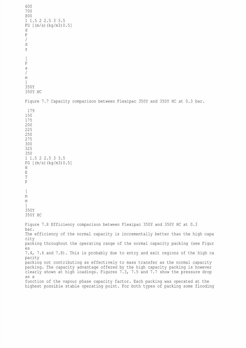
8/10/2019 Erasmus Mass 2004.PDF
http://slidepdf.com/reader/full/erasmus-mass-2004pdf 190/257
6007008001 1.5 2 2.5 3 3.5FG [(m/s)(kg/m3)0.5]dP/dz [Pa/m]350Y350Y HC Figure 7.7 Capacity comparison between Flexipac 350Y and 350Y HC at 0.3 bar.
179150
1752002252502753003253501 1.5 2 2.5 3 3.5FG [(m/s)(kg/m3)0.5]HET
P [mm]350Y350Y HC Figure 7.8 Efficiency comparison between Flexipac 350Y and 350Y HC at 0.3bar.The efficiency of the normal capacity is incrementally better than the high capacity
packing throughout the operating range of the normal capacity packing (see Figures7.4, 7.6 and 7.8). This is probably due to entry and exit regions of the high capacitypacking not contributing as effectively to mass transfer as the normal capacitypacking. The capacity advantage offered by the high capacity packing is howeverclearly shown at high loadings. Figures 7.3, 7.5 and 7.7 show the pressure dropas afunction of the vapour phase capacity factor. Each packing was operated at thehighest possible stable operating point. For both types of packing some flooding

8/10/2019 Erasmus Mass 2004.PDF
http://slidepdf.com/reader/full/erasmus-mass-2004pdf 191/257
wasobserved at the base of the bed or between packing elements at this operating point.The high capacity packing could be stably operated at vapour phase capacity factorsbetween 8% and 15% higher than was possible with the normal capacity packing. At an operating pressure of 1.0 bar, the increase in capacity is about 8% (see Figure7.3), while at an operating pressure of 0.3 bar the increase in capacity is in the orderof 15% (see Figure 7.7). This would suggest that the modifications to the entryandexit regions of the packing elements have a larger impact on capacity at highervapour velocities. There is also an increase in efficiency as the vapour loading isincreased. At the maximum loading where stable operation is still possible, theefficiency of the packing is retained and is similar to that obtained with the normal180packing at its maximum loading point where efficiency is still retained. What is alsonoteworthy is that the slope of the pressure drop curve in the loading region is
smaller for the high capacity packing compared to the normal packing. Visualinspection of the base of the structured packing elements showed the liquid drainageto be better for the high capacity packing than for the normal packing. At themaximum stable operating point of the normal packing there was a substantial heightof liquid suspended at the base of a packing element. For the high capacity packingthis height of liquid was considerably less. It is therefore expected that the efficiencyof the normal range of packing would deteriorate more rapidly because of backmixing than the high capacity packing as the flood point is approached. Becauseof
the smaller slope of the pressure drop curve in the loading region for the highcapacity packing, it would be possible to operate the column more stably at high loadings with this packing.7.6.2 Flexipac 350Y: Model predictionsPressure drop and holdupIn Figures 7.9 to 7.11 the experimentally determined pressure drops over Flexipac350Y are compared with the results obtained with the models evaluated in Chapter 4.Figure 7.9 compares the pressure drop calculated with the SRP model with theexperimental results at the different operating pressures. Figure 7.10 show theresults obtained with the Delft model and Figure 7.11 the results for the Billet
model.The experimental pressure drop shown in Figures 7.9 to 7.11 is the pressure drop over the packing. This pressure drop was calculated by subtracting the pressuredropover the liquid distributors and the static pressure drop from the experimentalmeasured pressure drop. A comparison between Figures 7.9 to 7.11 show that themodel by Billet is accurate in predicting the pressure drop in the preloading region(FG < 2.25). Both the SRP and Delft models predict the onset of loading conditio
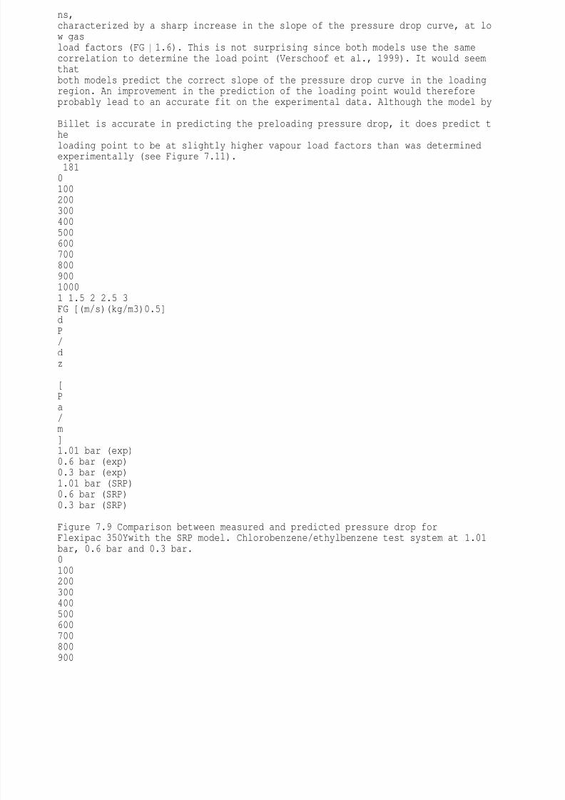
8/10/2019 Erasmus Mass 2004.PDF
http://slidepdf.com/reader/full/erasmus-mass-2004pdf 192/257
ns,characterized by a sharp increase in the slope of the pressure drop curve, at low gasload factors (FG 1.6). This is not surprising since both models use the samecorrelation to determine the load point (Verschoof et al., 1999). It would seemthatboth models predict the correct slope of the pressure drop curve in the loadingregion. An improvement in the prediction of the loading point would thereforeprobably lead to an accurate fit on the experimental data. Although the model by Billet is accurate in predicting the preloading pressure drop, it does predict theloading point to be at slightly higher vapour load factors than was determinedexperimentally (see Figure 7.11).1810100200300400500600700800
90010001 1.5 2 2.5 3FG [(m/s)(kg/m3)0.5]dP/dz [Pa
/m]1.01 bar (exp)0.6 bar (exp)0.3 bar (exp)1.01 bar (SRP)0.6 bar (SRP)0.3 bar (SRP) Figure 7.9 Comparison between measured and predicted pressure drop forFlexipac 350Ywith the SRP model. Chlorobenzene/ethylbenzene test system at 1.01bar, 0.6 bar and 0.3 bar.
0100200300400500600700800900
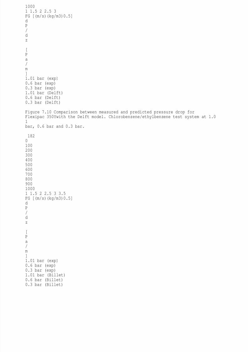
8/10/2019 Erasmus Mass 2004.PDF
http://slidepdf.com/reader/full/erasmus-mass-2004pdf 193/257
10001 1.5 2 2.5 3FG [(m/s)(kg/m3)0.5]dP/dz [Pa/m]1.01 bar (exp)0.6 bar (exp)0.3 bar (exp)1.01 bar (Delft)0.6 bar (Delft)0.3 bar (Delft) Figure 7.10 Comparison between measured and predicted pressure drop forFlexipac 350Ywith the Delft model. Chlorobenzene/ethylbenzene test system at 1.0
1bar, 0.6 bar and 0.3 bar.
1820100200300400500600700800
90010001 1.5 2 2.5 3 3.5FG [(m/s)(kg/m3)0.5]dP/dz [Pa
/m]1.01 bar (exp)0.6 bar (exp)0.3 bar (exp)1.01 bar (Billet)0.6 bar (Billet)0.3 bar (Billet)
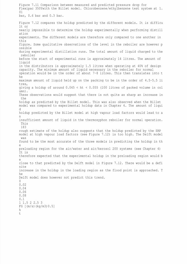
8/10/2019 Erasmus Mass 2004.PDF
http://slidepdf.com/reader/full/erasmus-mass-2004pdf 194/257
Figure 7.11 Comparison between measured and predicted pressure drop forFlexipac 350Ywith the Billet model. Chlorobenzene/ethylbenzene test system at 1.01bar, 0.6 bar and 0.3 bar.
Figure 7.12 compares the holdup predicted by the different models. It is difficult ornearly impossible to determine the holdup experimentally when performing distillationexperiments. The different models are therefore only compared to one another inthisfigure. Some qualitative observations of the level in the reboiler are however possibleduring experimental distillation runs. The total amount of liquid charged to the reboilerbefore the start of experimental runs is approximately 14 litres. The amount ofliquidin the distributors is approximately 1.5 litres when operating at 40% of designcapacity. The minimum amount of liquid necessary in the reboiler for normaloperation would be in the order of about 7-8 litres. This then translates into themaximum amount of liquid held up on the packing to be in the order of 4.5-5.5 litres,giving a holdup of around 0.045 < ht < 0.055 (100 litres of packed volume in col
umn).These observations would suggest that there is not quite as sharp an increase in theholdup as predicted by the Billet model. This was also observed when the Billetmodel was compared to experimental holdup data in Chapter 4. The amount of liquidholdup predicted by the Billet model at high vapour load factors would lead to aninsufficient amount of liquid in the thermosyphon reboiler for normal operation. This183rough estimate of the holdup also suggests that the holdup predicted by the SRPmodel at high vapour load factors (see Figure 7.12) is too high. The Delft model
wasfound to be the most accurate of the three models in predicting the holdup in thepreloading region for the air/water and air/kerosol 200 systems (see Chapter 4)It istherefore expected that the experimental holdup in the preloading region would beclose to that predicted by the Delft model in Figure 7.12. There would be a definiteincrease in the holdup in the loading region as the flood point is approached. TheDelft model does however not predict this trend.0
0.020.040.060.080.11 1.5 2 2.5 3FG [(m/s)(kg/m3)0.5]ht

8/10/2019 Erasmus Mass 2004.PDF
http://slidepdf.com/reader/full/erasmus-mass-2004pdf 195/257
[m3/m3]1.01 bar 0.6 bar 0.3 barBillet SRP Delft Figure 7.12 Holdup predicted by different models for Flexipac 350Y.Chlorobenzene/ethylbenzene test system at 1.01 bar, 0.6 bar and 0.3 bar.7.6.3 EfficiencyThe HETP predicted by the different models are compared with the experimentallydetermined HETP in Figures 7.13 to 7.15.1842002252502753003253501 1.5 2 2.5 3
FG [(m/s)(kg/m3)0.5]HETP [mm]1.01 bar (exp) 1.01 bar (SRP)0.6 bar (exp) 0.6 bar (SRP)0.3 bar (exp) 0.3 bar (SRP)
Figure 7.13 Efficiency of Flexipac 350Y predicted by the SRP model.Chlorobenzene/ethylbenzene test system at 1.01 bar, 0.6 bar and 0.3 bar.200225250275300325350375400425
4501 1.5 2 2.5 3FG [(m/s)(kg/m3)0.5]HETP [m

8/10/2019 Erasmus Mass 2004.PDF
http://slidepdf.com/reader/full/erasmus-mass-2004pdf 196/257
m]1.01 bar (exp) 1.01 bar (Delft)0.6 bar (exp) 0.6 bar (Delft)0.3 bar (exp) 0.3 bar (Delft) Figure 7.14 Efficiency of Flexipac 350Y predicted by the Delft model.Chlorobenzene/ethylbenzene test system at 1.01 bar, 0.6 bar and 0.3 bar.1851201451701952202452702953203451 1.5 2 2.5 3FG [(m/s)(kg/m3)0.5]HET
P [mm]1.01 bar (exp) 1.01 bar (Billet)0.6 bar (exp) 0.6 bar (Billet)0.3 bar (exp) 0.3 bar (Billet) Figure 7.15 Efficiency of Flexipac 350Y predicted by the Billet model.Chlorobenzene/ethylbenzene test system at 1.01 bar, 0.6 bar and 0.3 bar.The experimental determined efficiency show a decrease in HETP (increase in
efficiency) with an increase in the vapour load factor. A comparison between the efficiency calculated with the different models clearly shows that the SRP and Billetmodels predict this trend. The Delft model predicts a decrease in efficiency with anincrease in the vapour load factor (see Figure 7.14). It is expected that high up in theloading region the efficiency will start to decrease as the flood point is approached,but not over the entire operating range as predicted by the Delft model. Figures 7.13to 7.15 show that the SRP model is the most accurate of the three models in
predicting the efficiency of Flexipac 350Y. The model by Billet over predicts theefficiency and the Delft model under predicts the efficiency. The model by Billet alsopredicts a sharp rise in the efficiency in the loading region (see Figure 7.15). Although the efficiency does increase in the loading region, the increase is not asdramatic as suggested by the Billet model. It is difficult to compare the models based

8/10/2019 Erasmus Mass 2004.PDF
http://slidepdf.com/reader/full/erasmus-mass-2004pdf 197/257
on the overall efficiency shown in Figures 7.13 to 7.15. Since the overall efficiency iscalculated from the vapour- and liquid side mass transfer coefficients and theeffective surface area (see Chapter 2), it would be more appropriate to comparethemodel predictions of these quantities. Figure 7.16 shows the gas phase masstransfer coefficient (kG) predicted by the different models.18600.020.040.060.080.10.120.140.160.180.21 1.5 2 2.5 3FG [(m/s)(kg/m3)0.5]kG
[m/s]1.01 bar 0.6 bar 0.3 barBillet SRP Delft Figure 7.16 Vapour phase mass transfer coefficient predictions by SRP, Delft and Billet models for Flexipac 350Y. Chlorobenzene/ethylbenzene test system at 1.01bar, 0.6 bar and 0.3 bar.0
0.00020.00040.00060.00080.0010.00121 1.5 2 2.5 3FG [(m/s)(kg/m3)0.5]kL [m
/s]1.01 bar 0.6 bar 0.3 barBillet SRP Delft Figure 7.17 Liquid phase mass transfer coefficient predictions by SRP, Delft and Billet models for Flexipac 350Y. Chlorobenzene/ethylbenzene test system at 1.01bar, 0.6 bar and 0.3 bar.

8/10/2019 Erasmus Mass 2004.PDF
http://slidepdf.com/reader/full/erasmus-mass-2004pdf 198/257
187Figure 7.17 compares the liquid phase mass transfer coefficients (kL) and Figure 7.18the effective surface area (ae). Figures 7.16 to 7.18 show that the models differwidely in their predictions of mass transfer coefficients and effective surfacearea.The Billet model predicts extremely high vapour phase mass transfer coefficients compared to the SRP and Delft models. For an operating pressure of 1.01 bar, the vapour phase mass transfer coefficient predicted by the Billet model is almost threetimes higher than the vapour phase mass transfer coefficient predicted by the SRPmodel and almost six times higher than that predicted by the Delft model (Figure 7.16).
There are also large differences in the prediction of the liquid phase mass transfercoefficient. At an operating pressure of 1.01 bar the Billet prediction is on average afactor three higher than the SRP prediction. The liquid phase mass transfer
coefficient predicted the Delft model predicts about half of that by the Billetmodel.The sharp increase in the liquid phase mass transfer coefficient calculated with theBillet model is due to a sharp increase in the liquid holdup (see Figure 7.12).TheBillet model compensates for the very high mass transfer coefficients by predicting alow effective interfacial area, as shown in Figure 7.18. In calculating the effectiveinterfacial area in the Billet model, the increase in effective surface area intheloading region as suggested by Billet (Billet, 1995) was not included since this
led torather large and unrealistic values for the effective surface area. The Delft modelcompensates for the rather low vapour phase mass transfer coefficient by predictinga large effective surface area. This area is about 90% of the geometric specific surface area of the packing. The SRP effective surface area is about midwaybetween that predicted with the Billet and Delft models.
The reasons for these large differences are unclear. One possible reason may bethat volumetric mass transfer coefficients (kG.ae, kL.ae) were measuredexperimentally. These were then split up arbitrarily, or according to some kind
ofmodel, into mass transfer coefficients (kG, kL) and effective surface area (ae)andmodelled separately.188050100150200
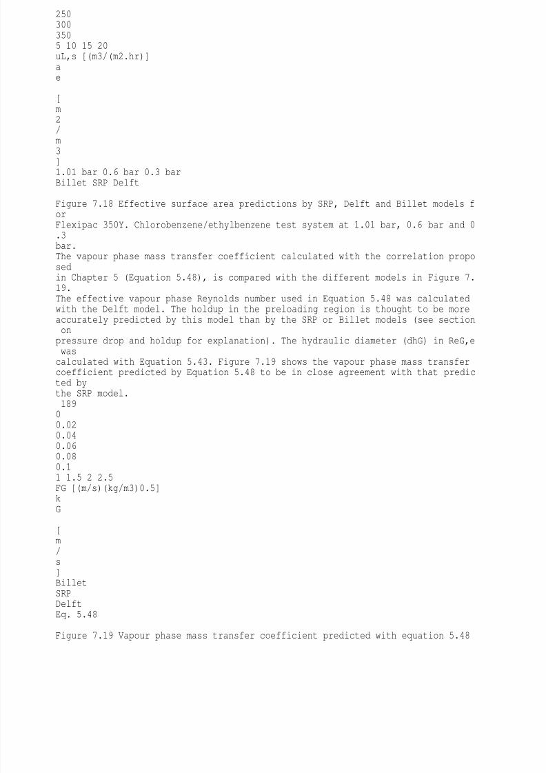
8/10/2019 Erasmus Mass 2004.PDF
http://slidepdf.com/reader/full/erasmus-mass-2004pdf 199/257
2503003505 10 15 20uL,s [(m3/(m2.hr)]ae [m2/m3]1.01 bar 0.6 bar 0.3 barBillet SRP Delft Figure 7.18 Effective surface area predictions by SRP, Delft and Billet models forFlexipac 350Y. Chlorobenzene/ethylbenzene test system at 1.01 bar, 0.6 bar and 0.3bar.The vapour phase mass transfer coefficient calculated with the correlation propo
sedin Chapter 5 (Equation 5.48), is compared with the different models in Figure 7.19.The effective vapour phase Reynolds number used in Equation 5.48 was calculatedwith the Delft model. The holdup in the preloading region is thought to be moreaccurately predicted by this model than by the SRP or Billet models (see section onpressure drop and holdup for explanation). The hydraulic diameter (dhG) in ReG,e wascalculated with Equation 5.43. Figure 7.19 shows the vapour phase mass transfercoefficient predicted by Equation 5.48 to be in close agreement with that predicted bythe SRP model.
18900.020.040.060.080.11 1.5 2 2.5FG [(m/s)(kg/m3)0.5]kG [
m/s]BilletSRPDelftEq. 5.48 Figure 7.19 Vapour phase mass transfer coefficient predicted with equation 5.48
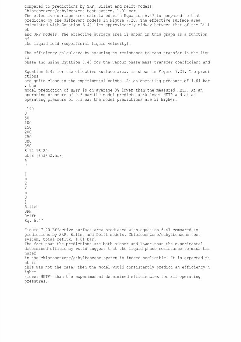
8/10/2019 Erasmus Mass 2004.PDF
http://slidepdf.com/reader/full/erasmus-mass-2004pdf 200/257
compared to predictions by SRP, Billet and Delft models.Chlorobenzene/ethylbenzene test system, 1.01 bar.The effective surface area calculated with Equation 6.47 is compared to thatpredicted by the different models in Figure 7.20. The effective surface areacalculated with Equation 6.47 lies approximately midway between that of the Billetand SRP models. The effective surface area is shown in this graph as a functionofthe liquid load (superficial liquid velocity).
The efficiency calculated by assuming no resistance to mass transfer in the liquidphase and using Equation 5.48 for the vapour phase mass transfer coefficient and Equation 6.47 for the effective surface area, is shown in Figure 7.21. The predictionsare quite close to the experimental points. At an operating pressure of 1.01 bar, themodel prediction of HETP is on average 9% lower than the measured HETP. At anoperating pressure of 0.6 bar the model predicts a 3% lower HETP and at anoperating pressure of 0.3 bar the model predictions are 5% higher.
1900
501001502002503003508 12 16 20uL,s [(m3/m2.hr)]ae [
m2/m3]BilletSRPDelftEq. 6.47 Figure 7.20 Effective surface area predicted with equation 6.47 compared topredictions by SRP, Billet and Delft models. Chlorobenzene/ethylbenzene test
system, total reflux, 1.01 bar.The fact that the predictions are both higher and lower than the experimentaldetermined efficiency would suggest that the liquid phase resistance to mass transferin the chlorobenzene/ethylbenzene system is indeed negligible. It is expected that ifthis was not the case, then the model would consistently predict an efficiency higher(lower HETP) than the experimental determined efficiencies for all operatingpressures.

8/10/2019 Erasmus Mass 2004.PDF
http://slidepdf.com/reader/full/erasmus-mass-2004pdf 201/257
1911802052302552803053301 1.5 2 2.5 3FG [(m/s)(kg/m3)0.5]HETP [mm]1.01 bar (exp) 1.01 bar (model)0.6 bar (exp) 0.6 bar (model)0.3 bar (exp) 0.3 bar (model) Figure 7.21 Efficiency of Flexipac 350Y predicted with kG and ae correlations
developed in this study. Chlorobenzene/ethylbenzene test system at 1.01 bar, 0.6 bar and 0.3 bar.7.7 ConclusionsFrom the results obtained in this chapter, the following conclusions may be drawn: The new high capacity structured packing Flexipac 350Y HC offers an increasein capacity of between 8% and 15% when compared with the normal capacitypacking Flexipac 350Y. Both Flexipac 350Y and 350Y HC could be operated stably at pressure drops ofaround 600 Pa/m without losing efficiency. It is expected that the high capacity packing could be operated stably at even higher pressure drops.
The SRP and Delft models predict the loading point of Flexipac 350Y at lowerthan measured vapour load factors. The Billet model is accurate in predicting thepreloading pressure drop. It predicts the loading point to be slightly higher thanwas determined experimentally. The liquid holdup predicted by the SRP and Billet models in the loading region istoo high when compared with rough experimental estimates. Overall the Delft model predicts an efficiency 46% lower than was determinedexperimentally for Flexipac 350Y. The efficiency predicted by the SRP model for192this packing is on average 13% lower. The Billet model predicts an efficiency th
atis on average 27% higher. The models differ widely in their predictions of liquid- and vapour phase masstransfer coefficients. This is a serious cause for concern. When ignoring liquid phase resistance and calculating the efficiency for Flexipac350Y with the correlations developed in this study for the vapour phase masstransfer coefficient and effective surface area, the predicted efficiency is 9%higher than that determined experimentally at 1.01 bar. At an operating pressure

8/10/2019 Erasmus Mass 2004.PDF
http://slidepdf.com/reader/full/erasmus-mass-2004pdf 202/257
of 0.6 bar, the predicted efficiency is on average 3% higher and at an operating pressure of 0.3 bar the predicted efficiency is on average 5% lower than theexperimentally determined efficiency.1937.8 Nomenclatureae Effective surface area of packing [m2/m3]ap Geometric area of packing [m2/m3]B Channel base dimension [m]D Diffusion coefficient [m2/s]dh Hydraulic diameter [m]FG Vapour capacity factor [(m/s)(kg/m3)0.5]Fr Froude number [-]FSE Discount factor for liquid phase mass transfer coefficient [-]h Channel crimp height [m]ht Total liquid holdup [m3/m3]k Mass transfer coefficient [m/s]
G,pe Length of triangular vapour phase channel [m]Re Reynolds number [-]S Side dimension of corrugated channel [m]Sc Schmidt number [-]Sh Sherwood number [-]u Velocity [m/s]We Weber number [-]
Greekp = 3.14159¼q Corrugation angle [o]m Dynamic viscosity [Pa.s]W Fraction of packing area occupied by holes [-]j Fraction of triangular passage occupied by liquid [-]xGL Vapour/liquid friction factor [-]e Void fraction [-]g Contact angle between solid and liquid [o]r Density [kg/m3]Subscriptse Effectivefp Refers to flood point
G Refers to vapour phase property194L Refers to liquid phase propertylam Laminar contributionlp Refers to loading points Superficialturb Turbulent contribution
1958 CONCLUSIONSThe ultimate goal of this study was to arrive at a model for the capacity and the
efficiency of the sheet metal structured packing Flexipac 350Y, with the emphasis onthe development of accurate correlations for modelling efficiency. In the followingparagraphs, the conclusions reached in the different chapters are discussed usingthese two goals (the modelling of capacity and efficiency) as main themes. Theincrease in capacity that the new high capacity packing offers is also discussed.

8/10/2019 Erasmus Mass 2004.PDF
http://slidepdf.com/reader/full/erasmus-mass-2004pdf 203/257
Since there are quite a few capacity models available in literature, no new model wasdeveloped. The existing models were tested against experimentally measuredhydrodynamic data and those more suitable were identified. From the resultsobtained with the different hydraulic models, the following conclusions may be drawn: The hydraulic capacity model by Stichlmair fails to predict the correctpressure drop trend for Flexipac 350Y. This is thought to be due to the factthat the model was fitted mainly on data for random packing The models by the SRP and Delft predict the onset of loading conditions atlower vapour loadings than were measured experimentally. The model byBillet predicts the load point at slightly higher vapour loads, but is moreaccurate than the SRP and Delft models. The Delft model is more accurate than the SRP and Billet models inpredicting the holdup in the preloading region. In the loading region both themodels of the SRP and Billet predicts too high a liquid holdup. The model by Billet is the most accurate in predicting the pressure drop in thepreloading region. All the models predict a conservative dependency of packing capacity onliquid viscosity.The efficiency of Flexipac 350Y was determined by performing total reflux distillationusing chlorobenzene/ethylbenzene as test system and modelled with differentefficiency models available in literature. The efficiency models differ widely i
n theirprediction of the mass transfer coefficients for the liquid- and vapour phases and theeffective surface area. In this study the vapour phase mass transfer coefficient andeffective surface area were measured and correlated independently from each other.From the experimental and modelling results for the efficiency of Flexipac 350Y, thefollowing conclusions may be drawn:196 For binary total reflux distillation using chlorobenzene/ethylbenzene as testsystem, the Delft model predicted an efficiency 46% lower than was
measured experimentally, the SRP model was on average 13% lower and theBillet model on average 27% higher. The sublimation of naphthalene from structured packing was used todetermine the vapour phase mass transfer coefficient. Although this is quitean old method to determine vapour phase mass transfer coefficients, it is thefirst time that this technique has been used to determine the vapour phasemass transfer coefficients in structured packing. The experimentallydetermined vapour phase mass transfer coefficient was correlated with:0.62 0.33G G,e GSh 0.3053Re Sc= The vapour phase mass transfer rate was found to be the same for thebottom- and top half of a structured packing element at low vapour phaseReynolds numbers. At vapour phase Reynolds numbers higher thanapproximately ReG,e = 6000, the vapour phase mass transfer rate is slightly
higher for the bottom half of the segment compared to the top half. CFD has been used in the past to determine the dry pressure drop throughpacking and to compare different designs based on the comparison ofmodelling of hypothetical heat transfer rates. To the author's knowledge, thisis the first time that CFD has been used to model real vapour phase masstransfer rates in structured packing. In the CFD modelling of structured packing it was necessary to model only asingle representative micro element. The BSL turbulence model of Menterwas successfully used in modelling the vapour phase mass transfer rate. Theresults obtained are sensitive to the placement of inlet- and outlet boundaries

8/10/2019 Erasmus Mass 2004.PDF
http://slidepdf.com/reader/full/erasmus-mass-2004pdf 204/257
for such a micro element. The absorption of CO2 into monoethanolamine with n-propanol as solventwas identified as an organic system for determining effective interfacial areain structured packing. To the author's knowledge this is the first time that anorganic system with both a low surface tension and low viscosity has beenused to determine effective surface area in structured packing. For systems with a low surface tension and a low viscosity, it is commonlybelieved that the effective surface area would be high. The effective surfacearea was, however, found to be substantially lower than expected. Theexperimental determined effective surface area of Flexipac 350Y shows a197logarithmic trend with increasing liquid load. The experimental results werecorrelated with:( )-= + · +3e L,spa 0.331 Ln u 1 10 2.29awhere uL,s is the superficial liquid velocity with units [m3/(m2.s)]. When ignoring liquid phase resistance and calculating the efficiency forFlexipac 350Y for the chlorobenzene/ethylbenzene test system with thecorrelations developed in this study, the predicted efficiency was 9% higherthan that determined experimentally at 1.01 bar. At an operating pressure of0.6 bar, the predicted efficiency was on average 3% higher and at anoperating pressure of 0.3 bar the predicted efficiency was on average 5%
lower than the experimentally determined efficiency. This is a substantialimprovement on existing models. These correlations may be used as a starting point in the development of anaccurate correlation for the liquid phase mass transfer coefficient.The capacity and efficiency of the high capacity packing Flexipac 350Y HC weremeasured experimentally and compared with the normal capacity packing Flexipac350Y. The following conclusions were reached: The high capacity packing used in this study showed a higher dry bedpressure drop compared to the normal capacity packing. This is thought to bedue to the slight difference in corrugation geometry between the two types ofpacking. There is an increase in capacity of 20% for the new packing compared withthe normal packing for the air/water system. The increase in capacity for
viscous liquid systems is only 4%. The new high capacity structured packing Flexipac 350Y HC offers anincrease in capacity of between 8% and 15% when compared with the normalcapacity packing Flexipac 350Y. When compared with the high capacity packing, the efficiency of the normalcapacity packing is incrementally better (around 3%) over the entire operatingrange of the normal capacity packing.From the above conclusions it is clear that the new high capacity packingFlexipac 350Y HC will perform as well or better than the normal capacity packing Flexipac 350Y. For systems where the liquid viscosity is low, as encountered inthe binary total reflux distillation work performed in this study, the increasein
capacity that the high capacity packing offers more than offsets the higher198efficiency of the normal capacity packing. For viscous systems it is expected thatthe performance of the two types of packing would be similar.
In summary this project has contributed to the current body of knowledge on theefficiency of structured packing by laying the foundations for an experimentalmethod to characterize packing efficiency. These experimental methods may beused to evaluate the efficiency of new packing designs, compare it with current

8/10/2019 Erasmus Mass 2004.PDF
http://slidepdf.com/reader/full/erasmus-mass-2004pdf 205/257
packing designs and identify areas where improvements may be possible. It hasalso highlighted the role that CFD may play in the development of vapour phasemass transfer correlations. The inability of current mass transfer models topredict the efficiency of structured packing has lead design engineers to uselarge safety factors when designing new colums. The correlations developed inthis study will hopefully contribute towards more accurate designs for columnscontaining structured packing. This will have a positive impact on the overallprocess economics.
199REFERENCES
Abbott, M. M. and Prausnitz, J. M. (1994). In Models for Thermodynamic and Phase Equilibria Calculations(Ed, Sandler, S. I.) Marcel Dekker, New York.
AEA Technology (2002). CFX-4.4. Harwell, UK.
Alvarez-Fuster, C., Midoux, N., Laurent, A. and Charpentier, J. C. (1980). "ChemicalKinetics of the Reaction of Carbon Dioxide with Amines in Pseudo m,nth OrderConditions in Aqueous and Organic Solutions", Chem. Eng. Sci., 35, 1717.
Alvarez-Fuster, C., Midoux, N., Laurent, A. and Charpentier, J. C. (1981). "ChemicalKinetics of the Reaction of CO2 with Amines in Pseudo m-nth Order Conditions inPolarand Viscous Organic Solutions", Chem. Eng. Sci., 36, 1513.
Ambrose, D., Lawrenson, I. J. and Sprake, C. H. S. (1975). "The vapour pressureofnaphthalene", J. Chem. Thermodynamics, 7, 1173.
ASME (1959). Fluid Meters: Their Theory and Application, The American Society of Mechanical Engineers, New York.
Astarita, G. (1967). Mass Transfer with Chemical Reaction, Elsevier, Amsterdam.
Ataki, A. and Bart, H. J. (2002). "Experimental Study of Rivulet Liquid Flow onanInclined Plate." International Conference on Distillation & Absorption, 634th event of theEuropean Federation of Chemical Engineering, Baden-Baden, Germany.
Bennett, D. L. and Ludwig, K. A. (1994). "Understand the Limitations of Air/WaterTesting of Distillation Equipment", Chem. Eng. Prog., 90, 72.
Billet, R. (1995). Packed Towers in Processing and Environmental Technology, VCH,Weinheim.
200Billingham, J. F. and Lockett, M. J. (1999). "Development of a New Generation of Structured Packings for Distillation", Trans. IChemE, 77, 583.
Bird, R. B., Stewart, W. E. and Lightfoot, E. N. (1960). Transport Phenomena, Jo
8/10/2019 Erasmus Mass 2004.PDF
http://slidepdf.com/reader/full/erasmus-mass-2004pdf 206/257
hnWiley & Sons, New York.
Blauwhoff, P. M. M., Versteeg, G. F. and Van Swaaij, W. P. M. (1982). "A Study on theReaction between CO2 and Alkanolamines in Aqueous Solutions", Chem. Eng. Sci., 39,207.
Boston, J. F. and Sullivan, S. L. (1972). "An Improved Algorithm for Solving MassBalance Equations in Multistage Separation Processes", Can. J. Chem. Eng., 50, 663.
Bratzler, K. and Doerges, A. (1974). "Amisol process purfies gases", Hydrocarbon Proc,1974, 78.
Bravo, J. L., Rocha, J. A. and Fair, J. R. (1985). "Mass transfer in gauze packings",Hydrocarbon Process., 64, 91.
Brunazzi, E. and Pagliante, A. (1997). "Mechanistic Pressure Drop Model for Columns
Containing Structured Packings", AIChE J., 43, 317.
Brunazzi, E. and Paglianti, A. (1997). "Liquid-Film Mass-Transfer Coefficient in a ColumnEquipped with Structured Packings", Ind. Eng. Chem. Res., 36, 3792.
Brunazzi, E., Nardini, G., Paglianti, A. and Petarca, L. (1995). "Interfacial Area ofMellapak Packing: Absorption of 1,1,1-Trichloroethane by Genosorb 300", Chem. Eng.Technol., 18, 248.
Charpentier, J. C. (1981). Mass Transfer Rates in Gas-Liquid Absorbers. In Advan
ces inChemical Engineering, Vol. 11 Academic Press, New York.
Chen, G. K., Kitterman, L. and Shieh, J. H. (1983). "High-Efficiency Packing for ProductSeparation", Chem. Eng. Prog., 79, 46.201
Chilton, T. H. and Colburn, A. P. (1935). "Distillation and Absorption in Packed Columns", Ind. Eng. Chem., 27, 255.
Cho, K., Irvine, T. F. j. and Karni, J. (1992). "Measurement of the diffusion co
efficient ofnaphthalene into air", Int. J. Heat Mass Transfer, 35, 957.
Ciofalo, M. (1996). "Large-eddy simulations of turbulent flow with heat transfer in simpleand complex geometries using Harwell-FLOW3D", Appl. Math. Modelling, 20, 262.
Ciofalo, M., Stasiek, J. and Collins, M. W. (1996). "Investigation of flow and heat transferin corrugated passages - 2. Numerical simulations", Int. J. Heat Mass Transfer,
8/10/2019 Erasmus Mass 2004.PDF
http://slidepdf.com/reader/full/erasmus-mass-2004pdf 207/257
39, 165.
Colburn, A. P. (1941). "Simplified Calculation of Diffusional Processes", Ind. Eng.Chem., 33, 459.
Coulson, J. M. and Richardson, J. F. (1991). Coulson & Richardson s ChemicalEngineering Vol 1, Butterworth Heinemann, Oxford.
Crause, J. C. (1998). A fundamental mass transfer model for an extractive distillationapplication. Stellenbosch, University of Stellenbosch.
Crause, J. C. and Nieuwoudt, I. (1999). "Mass Transfer in a Short Wetted-Wall Column.1. Pure Components", Ind. Eng. Chem. Res., 38, 4928.
Cussler, E. L. (1984). Diffusion: Mass Transfer in Fluid Systems, Cambridge UniversityPress, Cambridge.
Danckwerts, P. V. (1951). "Significance of Liquid Film Coefficients in Gas Absorption",Ind. Eng. Chem., 43, 1460.
Danckwerts, P. V. (1970). Gas-Liquid Reactions, McGraw-Hill, New York.
202Danckwerts, P. V. (1979). "The Reaction of CO2 with Ethanolamines", Chem. Eng. Sci.,34, 443.
Danckwerts, P. V. and Sharma, M. M. (1966). "The Absorption of Carbon Dioxide intoSolutions of Alkalis and Amines", The Chemical Engineer, 44, CE244.
Darton, R. C. (1992). "Distillation and Absorption Technology: Current Market an
d NewDevelopments", IChemE Symp. Ser., 128, A385.
Daugherty, R. L. and Franzini, J. B. (1977). Fluid Mechanics with EngineeringApplication, McGraw-Hill, Tokyo.
Davies, G. A., Ponter, A. B. and Craine, K. (1967). "The Diffusion of Carbon Dioxide inOrganic Liquids", Can. J. Chem. Eng., 45, 372.
Davis, R. A. and Sandall, O. C. (1993). "Kinetics of the Reaction of Carbon Dioxide withSecondary Amines in Polyethylene Glycol", Chem. Eng. Sci., 48, 3187.
De Brito, M. H., Von Stockar, U., Bangerter, A. M., Bomio, P. and Laso, M. (1994)."Effective Mass-Transfer Area in a Pilot Plant Column Equipped with StructuredPackings and with Ceramic Rings", Ind. Eng. Chem. Res., 33, 647.
Deibele, L. (1991). "Die Entwicklung der Destillationstechnik von ihren Anfangen bis zumJahre 1800", Chem. Ing. Tech., 63, 458.

8/10/2019 Erasmus Mass 2004.PDF
http://slidepdf.com/reader/full/erasmus-mass-2004pdf 208/257
Deibele, L. (1994). "Die Entwicklung der Destillationstechnik im 19. Jahrhundert", Chem.Ing. Tech., 66, 809.
Dudukovic, A., Milosevic, V. and Pjanovic, R. (1996). "Gas-Solid and Gas-LiquidMass-Transfer Coefficients", AIChE J., 42, 269.
Emmert, R. E. and Pigford, R. L. (1954). "Interfacial resistance", Chem. Eng. Progr., 50,87.203Erasmus, A. B. (1999). Mass Transfer in Structured Packing. University of Stellenbosch,Stellenbosch.
Erasmus, A. B. and Nieuwoudt, I. (2001). "Mass transfer in structured packing: A wetted-wall study", Ind. Eng. Chem. Res., 40, 2310.
Fair, J. R. and Bravo, J. L. (1990). "Distillation columns containing structured packing",Chem. Eng. Prog., January, 19.
Fair, J. R., Seibert, A. F., Behrens, M., Saraber, P. P. and Olujic, Z. (2000)."StructuredPacking Performance - Experimental Evaluation of Two Predictive Models", Ind. Eng.Chem. Res, 39, 1788.
Ferzigier, J. H. and Peric, M. (1996). Computational Methods for Fluid Mechanics,Springer, Berlin.
Focke, W. W., Zachariades, J. and Olivier, I. (1985). "The effect of the corrugationinclination angle on the thermohydraulic performance of plate heat exchangers",
Int. JHeat Mass Transfer, 28, 1469.
Foust, A. S., Wentzel, L. A., Clump, C. W., Maus, L. and Anderson, L. B. (1980). Principles of Unit Operations, John Wiley & Sons, New York.
Gilliland, E. R. and Sherwood, T. K. (1934). "Diffusion of vapors into an air stream", Ind.Eng. Chem., 26, 516.
Henley, E. J. and Seader, J. D. (1981). Equilibrium-Stage Operations in Chemical
Engineering, Wiley, New York.
Higler, A., Krishna, R. and Taylor, R. (1999a). "Nonequilibrium Cell Model forMulticomponent (Reactive) Separation Processes", AIChE J., 45, 2357.
Higler, A., Krishna, R. and Taylor, R. (1999b). "Nonequilibrium Cell Model for PackedDistillation Columns - The Influence of Maldistribution", Ind. Eng. Chem. Res.,38, 3988.204

8/10/2019 Erasmus Mass 2004.PDF
http://slidepdf.com/reader/full/erasmus-mass-2004pdf 209/257
Higler, A., Taylor, R. and Krishna, R. (1998). "Modeling of a Reactive SeparationProcess Using a Nonequilibrium Stage Model", Computers Che. Engng., 22, S111.
Hikita, H. and Asai, S. (1964). Int. Chem. Eng., 4, 332.
Hirsch, C. (1988). Numerical Computation of Internal and External Flows, John Wiley &Sons, New York.
Hodson, J. (1997). Computational Fluid Dynamical Studies of Structured DistillationPackings. University of Aston, Birmingham, UK.
Hodson, J. S., Fletcher, J. P. and Porter, K. E. (1997). "Fluid Mechanical Studies ofStructured Distillation Packings", IChemE Symp. Series, 142, 999.
Holland, C. D. (1975). Fundamentals and Modelling of Separation Processes, Prentice-Hall, New York.
Iliuta, I. and Larachi, F. (2001). "Mechanistic Model for Structured-Packing-Con
tainingColumns: Irrigated Pressure Drop, Liquid Holdup, and Packing Fractional Wetted Area",Ind. Eng. Chem. Res., 40, 5140.
Incropera, F. P. and De Witt, D. P. (1990). Fundamentals of Heat and Mass Transfer,Wiley, New York.Johnstone, H. F. and Pigford, R. L. (1942). Trans. Am. Inst. Chem. Engrs., 38, 25.
Jones, W. P. and Launder, B. E. (1972). "The Prediction of Laminarization with a Two-
Equation Model of Turbulence", Int. J. Heat Mass Transfer, 15, 301.
Karimi, G. and Kawaji, M. (1999). "Flow charateristics and circulatory motion in wavyfalling films with and without counter-current gas flow", Int. J. Multiphase Flow, 25, 1305.
King, C. J. (1980). Separation Processes, McGraw-Hill, New York.
205Kister, H. Z. (1992). Distillation Design, McGraw-Hill, New York.
Kister, H. Z. and Gill, D. R. (1992). In Distillation and Absorption 1992, Vol.
1Hemisphere, Birmingham, pp. A109.
Krishna, R. (1977). "A Generalized Film Model for Mass Transfer in Non-Ideal FluidMixtures", Chem. Eng. Sci., 32, 659.
Krishna, R. and Standart, G. L. (1976). "A Multicomponent Film Model Incorporating anExact Matrix Method of Solution to the Maxwell-Stefan Equations", AIChE J, 22, 3
8/10/2019 Erasmus Mass 2004.PDF
http://slidepdf.com/reader/full/erasmus-mass-2004pdf 210/257
83.
Krishna, R. and Standart, G. L. (1979). "Mass and Energy Transfer in MulticomponentSystems", Chem. Eng. Commun., 3, 201.
Krishna, R., Martinez, H. F., Sreedhar, R. and Standart, G. L. (1977). "Murphree PointEfficiencies in Multicomponent Systems", Trans. Inst. Chem. Engrs., 55, 178.
Krishna, R., Van Baten, J. M., Ellenberger, J., Higler, A. P. and Taylor, R. (1999). "CFDSimulations of Sieve Tray Hydrodynamics", Trans. IChemE, 77, 639.
Krishnamurthy, R. and Taylor, R. (1985a). "A Nonequilibrium Stage Model ofMulticomponent Separation Processes. Part 1: Model Description and Method ofSolution", AIChE J., 31, 449.
Krishnamurthy, R. and Taylor, R. (1985b). "A Nonequilibrium Stage Model ofMulticomponent Separation Processes. Part 2: Comparison with Experiment", AIChEJ.,31, 456.
Krishnamurthy, R. and Taylor, R. (1985c). "A Nonequilibrium Stage Model of
Multicomponent Separation Processes. Part 3: The Influence of Unequal Component-Efficiencies in Process Design Problems", AIChE J., 31, 1973.
Larachi, F., Petre, C. F., Iliuta, I. and Grandjean, B. (2003). "Tailoring the pressure dropof structured packing through CFD simulations", Chem. Eng. Proc., 42, 535.206
Laso, M., De Brito, M. H., Bomio, P. and Von Stockar, U. (1995). "Liquid-side masstransfer characteristics of a structured packing", Chem. Eng. J., 58, 251.
Levich, V. G. (1962). Physicochemical Hydrodynamics, Prentice-Hall, New York.
Littel, R. J., Versteeg, G. F. and Van Swaaij, W. P. M. (1992). "Kinetics of CO2 withPrimary and Secondary Amines in Aqueous Solutions - I. Zwitterion DeprotonationKinetics for DEA and DIPA in Aqueous Blends of Alkanolamines", Chem. Eng. Sci., 47,2027.
McNulty, K. J. and Hsieh, C. L. (1982). "Hydraulic Performance and Efficiency of KochFlexipac Structured Packings." AIChE Annual Meeting, Los Angeles, California.
Menter, F. R. (1992). "Influence of Freestream Values on k-w Turbulence Model
Predictions", AIAA J., 30, 1657.
Menter, F. R. (1994). "Two-Equation Eddy-Viscosity Turbulence Models for EngineeringApplications", AIAA J., 32, 1598.Menter, F. R. and Grotjans, H. (2000). In Calculation of Complex Turbulent Flows (Ed,Tzabiras, G.) WIT Press, Southampton.
Mohamed Ali, A., Jansens, P. and Olujic, Z. (2002). "Experimental Characterisati
8/10/2019 Erasmus Mass 2004.PDF
http://slidepdf.com/reader/full/erasmus-mass-2004pdf 211/257
on andCFD Simulation of Gas Distribution Performance of Liquid (Re)Distributors andCollectors in Packed Columns." International Conference on Distillation & Absorption,Baden-Baden, Germany.
Naphtali, L. M. and Sandholm, D. P. (1971). "Multicomponent Separation Calculations byLinearization", AIChE J., 17, 148.
Nawrocki, P. A. and Chuang, K. T. (1996). "Carbon Dioxide Absorption into a StableLiquid Rivulet", Can. J. Chem. Eng., 74, 247.
207Nawrocki, Z. A., XU, Z. P. and Chuang, K. T. (1991). "Mass Transfer in StructuredCorrugated Packing", Can. J. Chem. Eng., 69, 1336.
Nesic, S. and Postlethwaite, J. (1992). "Calculation of wall-mass transfer rates inseparated flow using a low Reynolds number k-e model", Int. J. Heat Mass Transfer, 35,1977.
Nesic, S., Adamopoulos, G., Postlethwaite, J. and Bergstrom, D. J. (1993). "Modelling ofTurbulent Flow and Mass Transfer with Wall Function and Low-Reynolds NumberClosures", Can. J. Chem. Eng., 71, 28.
Nieuwoudt, I. (2001). "Structured packing evaluation 350Y HC & 350Y", Confidentialresearch report, Institute for Thermal Separations, Stellenbosch.
Nieuwoudt, I. (December 2003). Private communication.
Olujic, Z. (1997). "Development of a Complete Simulation Model for Predicting th
eHydraulic and Separation Performance of Distillation Columns Equipped with StructuredPackings.", Chem. Biochem. Eng. Q., 11, 31.
Olujic, Z., Kamerbeek, A. B. and De Graauw, J. (1999). "A corrugation geometry basedmodel for the efficiency of structured distillation packing", Chem. Eng. Process., 38, 683.
Onken, U. and Arlt, W. (1990). Recommended Test Mixtures for Distillation Columns,The Institution of Chemical Engineers, Rugby, Warwickshire, England.
Patankar, S. V. (1980). Numerical Heat Transfer and Fluid Flow, McGraw-Hill, New York.
Patel, V. C., Rodi, W. and Scheurer, G. (1985). "Turbulence Models for Near-Wall andLow Reynolds Number Flows: A Review", AIAA J., 23, 1308.
208
8/10/2019 Erasmus Mass 2004.PDF
http://slidepdf.com/reader/full/erasmus-mass-2004pdf 212/257
Petre, C. F., Larachi, F., Iliuta, I. and Grandjean, B. P. A. (2003). "Pressuredrop throughstructured packings: Breakdown into the contributing mechanisms by CFD modeling",Chem. Eng. Sci., 58, 163.
Porta (1553). Natural Magic, Naples.
Powers, M. F., Vickery, D. J., Arehole, A. and Taylor, R. (1988). "A Nonequilibrium StageModel of Multicomponent Separation Processes - V. Computational Methods for Solvingthe Model Equations", Comput. Chem. Engng., 12, 1229.
Ranke, H., Lerzer, R. and Becker, O. (2000). "Hydraulic Calculations for Cross-channeled Packings in Distillation Units Based on a Physical Model", Chem. Eng.Technol., 23, 691.
Reid, R. C., Prausnitz, J. M. and Polling, B. E. (1986). The Properties of Gases andLiquids, McGraw-Hill, New York.
Rhie, C. M. and Chow, W. L. (1983). "Numerical Study of the Turbulent Flow Pastan
Airfoil with Trailing Edge Separation", AIAA J., 21, 1525.
Rieger, R., Weiss, C., Wigley, G., Bart, H. J. and Marr, R. (1996). "Investigating theProcess of Liquid-Liquid Extraction by Means of Computational Fluid Dynamics",Computers Chem. Engng., 20, 1467.
Robbins, L. A. (1991). "Improve Pressure-Drop Prediction With a New Correlation",Chem. Eng. Prog., 87.
Roberts, D. and Danckwerts, P. V. (1962). "Kinetics of CO2 absorption in alkaline
solutions - I Transient absorption rates and catalysis by arsenite", Chem. Eng.Sci., 17,961.
Rocha, J. A. and Bravo, J. L. (1996). "Distillation Columns Containing Strutured Packings: A comprehensive Model for their performance. 2. Mass-Transfer Model",Ind.Eng. Chem. Res., 35, 1660.209
Rocha, J. A., Bravo, J. L. and Fair, J. R. (1993). "Distillation Columns Containing
Structured Packings: A Comprehensive Model for Their Performance. 1. HydraulicModels", Ind. Eng. Chem. Res., 32, 641.
Rocha, J. A., Bravo, J. L. and Fair, J. R. (1993). "Distillation Columns ContainingStructured Packings: A Comprehensive Model for Their Performance. 1. HydraulicModels", Ind. Eng. Chem. Res., 32, 641-651.
Sada, E., Kumazawa, H. and Butt, M. A. (1976). "Gas Absorption with ConsecutiveChemical Reaction: Absorption of Carbon Dioxide into Aqueous Amine Solutions", C
8/10/2019 Erasmus Mass 2004.PDF
http://slidepdf.com/reader/full/erasmus-mass-2004pdf 213/257
an.J. Chem. Eng., 54, 421.
Sada, E., Kumazawa, H., Han, Z. Q. and Matsuyama, H. (1985). "Chemical Kineticsofthe Reaction of Carbon Dioxide with Ethanolamines in Nonaqueous Solvents", AIChE J.,31, 1297.
Sada, E., Kumazawa, H., Ikehara, Y. and Han, Z. Q. (1989). "Chemical Kinetics of theReaction of Carbon Dioxide with Triethanolamine in Non-aqueous Solvents", Chem.Eng. J., 40, 7.
Sada, E., Kumazawa, H., Osawa, Y., Matsuura, M. and Han, Z. Q. (1986). "Reaction Kinetics of Carbon Dioxide with Amines in Non-aqueous Solvents", Chem. Eng. J.,33,87.
Schlichting, H. (1979). Boundary Layer Theory, McGraw-Hill, New York.
Seader, J. D. and Henley, E. J. (1998). Separation Process Principles, John Wiley &
Sons, New York.
Shahi, P., Hu, Y. and Chakma, A. (1994). "Gas chromatographic analysis of acid gasesand single/mixed alkanolamines", J. Chromatogr. A, 687, 121.
Shanley, A. (2000). "CFD for the Real World", Chemical Engineering, October, 139.210
Sharma, M. M. and Danckwerts, P. V. (1970). "Chemical methods of measuringinterfacial area and mass transfer coefficients in two-fluid systems.", BritishChem. Eng.,
15, 522.
Sherwood, T. K., Pigford, R. L. and Wilke, C. R. (1975). Mass Transfer, McGraw-Hill,New York.
Shetty, S. and Cerro, R. L. (1997). "Fundamental Liquid Flow Correlations for theComputation of Design Parameters for Ordered Packings", Ind. Eng. Chem. Res., 36,771.
Shi, M. G. and Mersmann, A. (1985). "Effective Interfacial Area in Packed Column
s",Ger. Chem. Eng., 8, 87.
Shulman, H. L., Ullrich, C. F., Proulx, A. Z. and Zimmerman, J. O. (1955). "Wetted andEffective-interfacial Areas, Gas- and Liquid-phase Mass Transfer Rates", AIChE J., 1,253.
Sideman, S. and Pinczewski, W. V. (1975). Turbulent Heat and Mass Transfer at

8/10/2019 Erasmus Mass 2004.PDF
http://slidepdf.com/reader/full/erasmus-mass-2004pdf 214/257
Interfaces: Transport Models and Mechanisms. In Transport Phenomena (Ed, Gutfinger,C.) Hemisphere, Washington.
Spiegel, L. and Meier, W. (1987). "Correlations of the performance characteristics of thevarious Mellapak types", Inst. Chem. Eng. Symp. Ser., 104, A203.
Sridharan, K. and Sharma, M. M. (1976). "New Systems and Methods for theMeasurement of Effective Interfacial Area and Mass Transfer Coefficients in Gas-LiquidContactors", Chem. Eng. Sci., 31, 767.
Stasiek, J., Collins, M. W., Ciofalo, M. and Chew, P. E. (1996). "Investigationof flow andheat transfer in corrugated passages - 1. Experimental results", Int. J. Heat MassTransfer, 39, 149.
211Stephan, K. and Hildwein, H. (1987). Recommended Data of Selected Compounds andBinary Mixtures, Dechema, Frankfurt.
Stichlmair, J., Bravo, J. L. and Fair, J. R. (1989). "General model for predicti
on ofpressure drop and capacity of countercurrent gas/liquid packed columns", Gas Sep.Purif., 3, 19.
Stirba, C. and Hurt, D. M. (1955). "Turbulence in falling liquid films", AIChE J., 1, 178-184.
Stoter, C. F. (1993). Modelling of Maldistribution in Structured Packings: Fromdetail tocolumn design. Delft University of Technology, Delft.
Suess, P. and Spiegel, L. (1992). "Hold-up of Mellapak structured packings", Chem.Eng. Process., 31, 119.
Taylor, R. and Krishna, R. (1993). Multicomponent Mass Transfer, John Wiley & Sons,New York.
Taylor, R., Kooijman, H. A. and Hung, J.-S. (1994). "A Second GenerationNonequilibrium Model for Computer Simulation of Multicomponent SeparationProcesses", Computers Chem. Engng., 18, 205.
Tomich, J. F. (1970). "A New Simulation Method for Equilibrium Stage Process", A
IChEJ., 16, 229.
Toor, H. L. and Marchello, J. M. (1958). "Film-penetration Model for Mass and HeatTransfer", AIChE J, 4, 97.
Van Baten, J. M., Ellenberger, J. and Krishna, R. (2001). "Radial and axial dispersion ofthe liquid phase within a KATAPAK-S structure: experiments vs. CFD simulations",
8/10/2019 Erasmus Mass 2004.PDF
http://slidepdf.com/reader/full/erasmus-mass-2004pdf 215/257
Chem. Eng. Sci., 56, 813.
212Van Doormal, J. P. and Raithby, G. D. (1984). "Enhancements to the SIMPLE Method for Predicting Incompressible Fluid Flows", Numer. Heat Transfer, 7, 147.
Verschoof, H.-J., Olujic, Z. and Fair, J. R. (1999). "A General Correlation forPredictingthe Loading Point of Corrugated Sheet Structured Packings", Ind. Eng. Chem. Res., 38,3663-3669.Versteeg, G. F. and Van Swaaij, P. M. (1988). "On the Kinetics between CO2 andAlkanolamines both in aqueous and Non-aqueous Solutions - I. Primary and SecondaryAmines", Chem. Eng. Sci., 43, 573.
Vogelpohl, A. (1979). "Murphree Efficiencies in Multicomponent Systems", Int. Chem.Eng. Symp. Ser., 56, 25.
Wall, J. (1975). "Gas Processing Handbook", Hydrocarbon Process, 54, 79.
Wang, J. and Shirazi, S. A. (2001). "A CFD based correlation for mass transfercoefficient in elbows", Int. J. Heat Mass Transfer, 44, 1817.
Wang, J. C. and Henke, G. E. (1966). "Tridiagonal Matrix for Distillation", HydrocarbonProcess., August, 155.
Wehrli, M., Hirschberg, S. and Schweizer, R. (2002). " Influence of Vapor Feed Designon the Flow Distribution." In International Conference on Distillation & Absorption, 634thevent of the European Federation of Chemical Engineering, Baden-Baden, Germany.
Weiland, R. H., Ahlgren, K. R. and Evans, M. (1993). "Mass-Transfer Characteristics ofSome Structured Packings", Ind. Eng. Chem. Res., 32, 1411.
Weimer, T. and Schaber, K. (1997). " Absorption of CO2 from the atmosphere as a method for the estimation of effective interfacial areas in packed columns." InDistillationand Absorption 97(Ed, Darton, R.) IChemE.
Wesselingh, J. A. (1997). "Non-Equilibrium Modelling of Distillation", Trans. IChemE, 75,529.
213Whitman, W. G. (1923). "The Two-film Theory of Absorption", Chem. Met. Eng., 29, 146.
Wilcox, D. C. (1988). "Reassessment of the Scale Determining Equation for AdvancedTurbulence Models", AIAA J., 26, 1299.
Wilcox, D. C. (1993a). "Comparison of Two-Equation Turbulence Models for Boundary

8/10/2019 Erasmus Mass 2004.PDF
http://slidepdf.com/reader/full/erasmus-mass-2004pdf 216/257

8/10/2019 Erasmus Mass 2004.PDF
http://slidepdf.com/reader/full/erasmus-mass-2004pdf 217/257
¶ ¶¶ ¶ ¶ ¶ m + + + + + ¶ ¶ ¶ ¶ ¶ 
8/10/2019 Erasmus Mass 2004.PDF
http://slidepdf.com/reader/full/erasmus-mass-2004pdf 218/257
(A1.1)Model constants:C 0.09m = kt 1.0s = t 1.3es = 1C 1.44e = 2C 1.92e = (A1.2)
A2 The k-w modelProduction term:( )( ) ( ) k32 P TTtk +m-+ = UUUUU (A1.3)Model Constants:0 T kT kRe R1 Re R** a +a = + (A1.4)0 TTRe R5 19 1 Re Rw*wa +a =+ a (A1.5))( )
( )4T4T5 18 Re R9100 1 Re Rb*b+b =+ (A1.6)
3 40b = kt 0.5s = t 0.5ws = 0 3*a = b 0 0.1a =R 8.0b = kR 6.0= R 2.7w = (A1.7)The turbulence Reynolds number is defined as:tkRe r=wm (A1.8)215A3 The BSL modelProduction term:( )( ) ( ) k32 P TTtk +m-+ = UUUUU (A1.9)The constants for set 1 (C1) are:kt1 0.5s = t1 0.5ws = 1 0.075b =0.09*b = 0.41k = t 21 1 1* *wg = b b - s k b (A1.10)
The constants for set 2 (C2) are:kt2 1.0s = t2 0.856ws = 2 0.0828b =0.09*b = 0.41k = t 22 2 2* *wg = b b - s k b (A1.11)The following definitions also apply:tkn =w (A1.12)( )41 1F tanh arg= (A1.13)wheret 2

8/10/2019 Erasmus Mass 2004.PDF
http://slidepdf.com/reader/full/erasmus-mass-2004pdf 219/257
1 2 2k4 kk 500arg min max ; ;0.09 y y CD yww
rsn= ww
8/10/2019 Erasmus Mass 2004.PDF
http://slidepdf.com/reader/full/erasmus-mass-2004pdf 220/257
(A1.14)andt 20k 2 1CD max 2 k ;10-w w = rs w w
(A1.15)y is the distance to the nearest wall.216APPENDIX B
Table B.1 SRP model equations(A) Hydraulic diameterVapour phase:( )- d=
- d - d - d + +
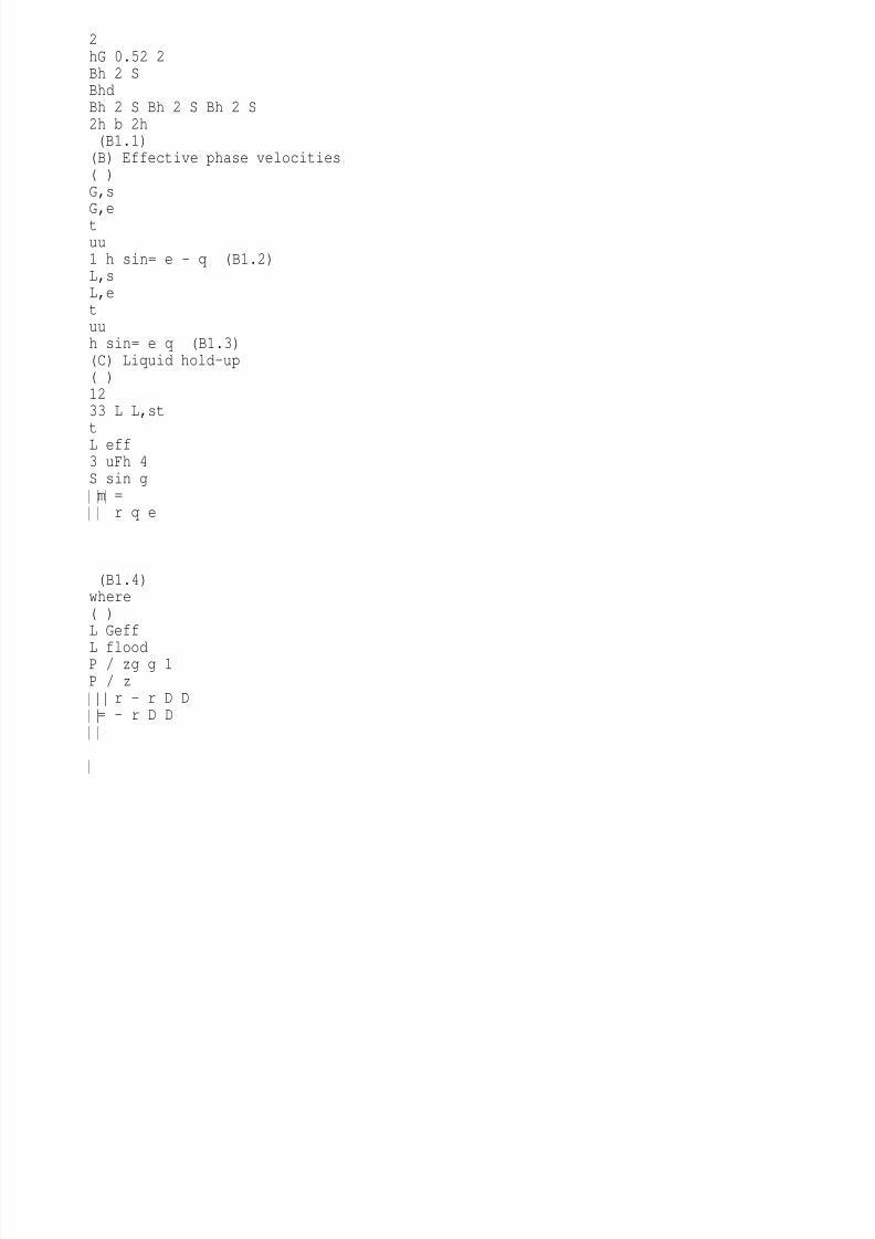
8/10/2019 Erasmus Mass 2004.PDF
http://slidepdf.com/reader/full/erasmus-mass-2004pdf 221/257
2hG 0.52 2Bh 2 SBhdBh 2 S Bh 2 S Bh 2 S2h b 2h (B1.1)(B) Effective phase velocities( )G,sG,etuu1 h sin= e - q (B1.2)L,sL,etuuh sin= e q (B1.3)(C) Liquid hold-up( )1233 L L,st
tL eff3 uFh 4S sin g
m = r q e
(B1.4)where( )L Geff
L floodP / zg g 1P / z
r - r D D = - r D D
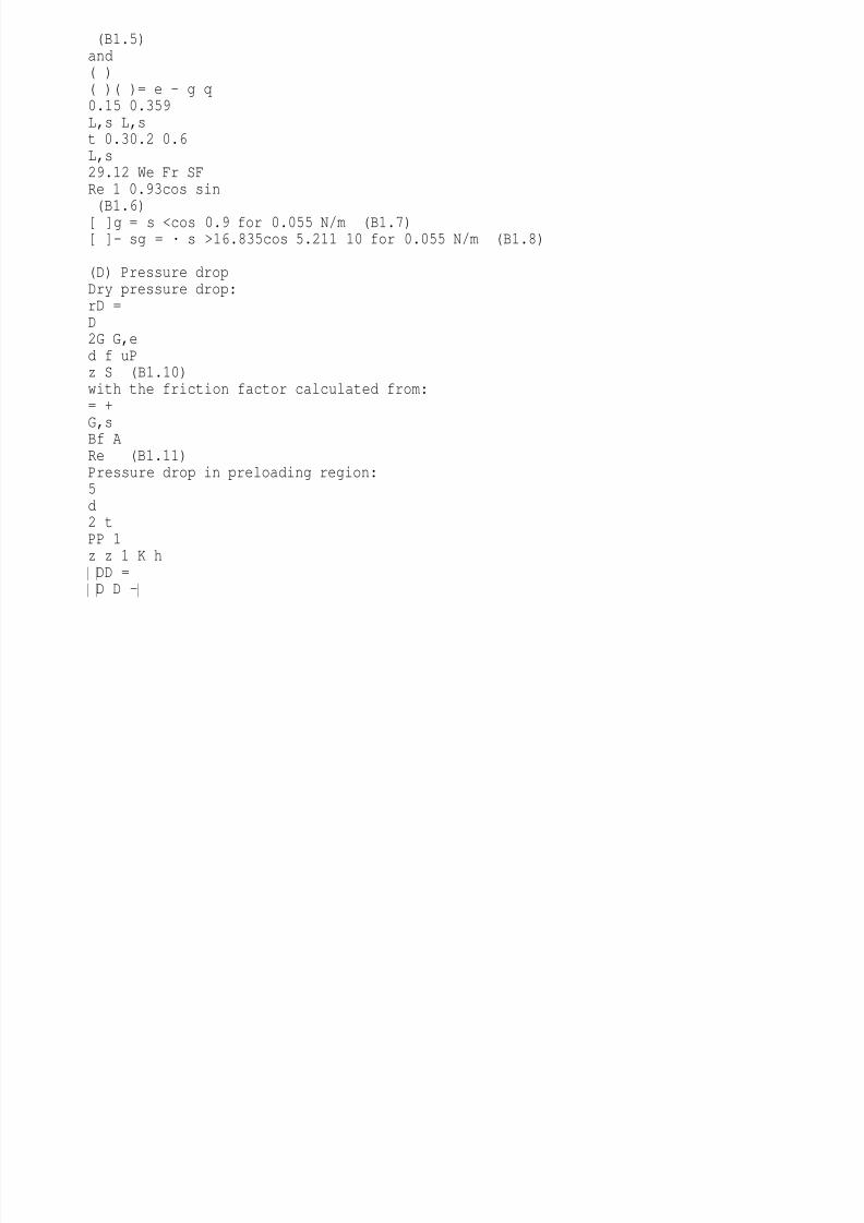
8/10/2019 Erasmus Mass 2004.PDF
http://slidepdf.com/reader/full/erasmus-mass-2004pdf 222/257
(B1.5)and( )( )( )= e - g q0.15 0.359L,s L,st 0.30.2 0.6L,s29.12 We Fr SFRe 1 0.93cos sin (B1.6)[ ]g = s <cos 0.9 for 0.055 N/m (B1.7)[ ]- sg = · s >16.835cos 5.211 10 for 0.055 N/m (B1.8)
(D) Pressure dropDry pressure drop:rD =D2G G,ed f uPz S (B1.10)with the friction factor calculated from:= +
G,sBf ARe (B1.11)Pressure drop in preloading region:5d2 tPP 1z z 1 K h
DD = D D -
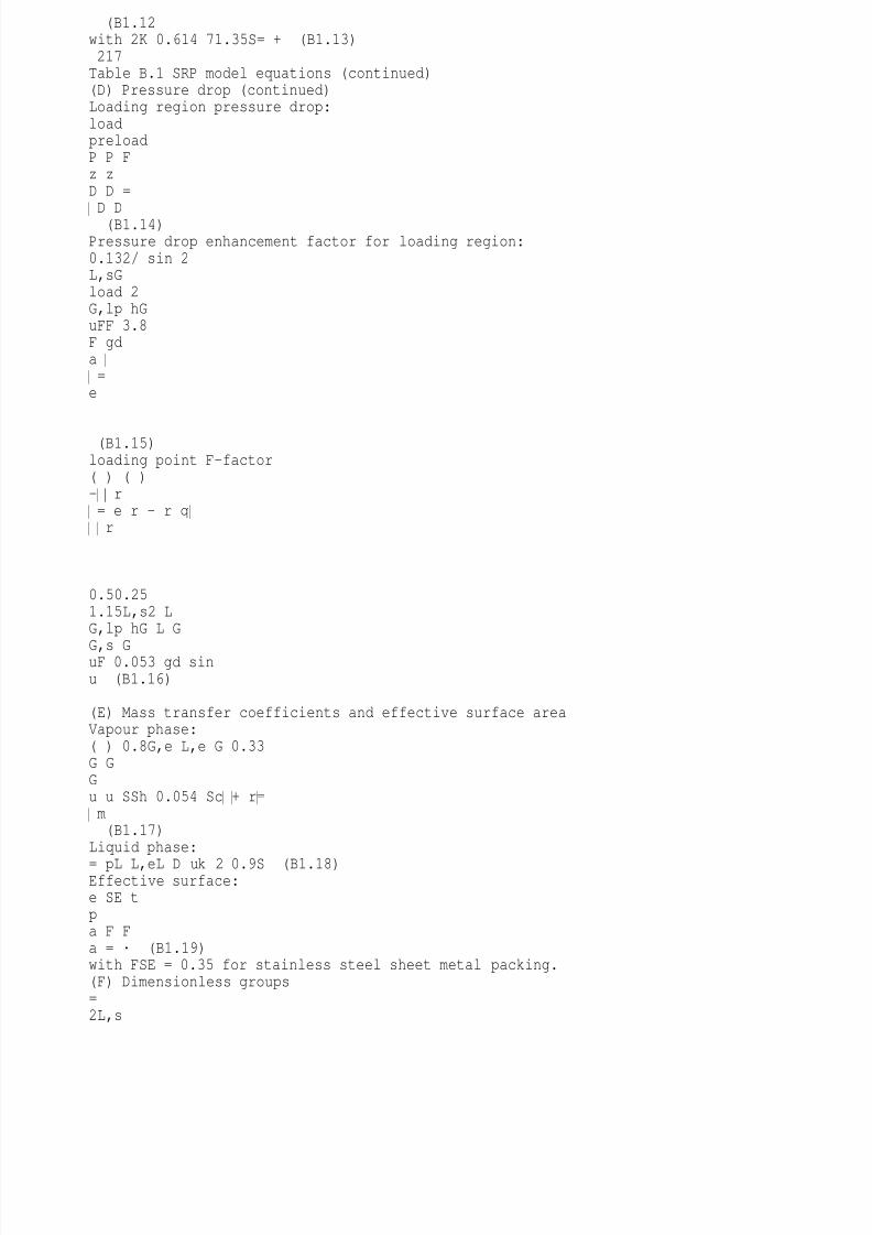
8/10/2019 Erasmus Mass 2004.PDF
http://slidepdf.com/reader/full/erasmus-mass-2004pdf 223/257
(B1.12with 2K 0.614 71.35S= + (B1.13)217Table B.1 SRP model equations (continued)(D) Pressure drop (continued)Loading region pressure drop:loadpreloadP P Fz zD D =
D D(B1.14)
Pressure drop enhancement factor for loading region:0.132/ sin 2L,sGload 2G,lp hGuFF 3.8F gda
= e
(B1.15)loading point F-factor( ) ( )- r
= e r - r q r
0.50.251.15L,s2 LG,lp hG L G
G,s GuF 0.053 gd sinu (B1.16)
(E) Mass transfer coefficients and effective surface areaVapour phase:( ) 0.8G,e L,e G 0.33G GGu u SSh 0.054 Sc + r =
m(B1.17)
Liquid phase:
= pL L,eL D uk 2 0.9S (B1.18)Effective surface:e SE tpa F Fa = · (B1.19)with FSE = 0.35 for stainless steel sheet metal packing.(F) Dimensionless groups=2L,s
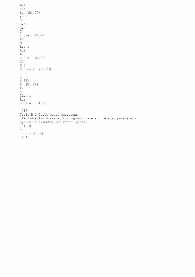
8/10/2019 Erasmus Mass 2004.PDF
http://slidepdf.com/reader/full/erasmus-mass-2004pdf 224/257
L,suFrSg (B1.20)r=mG,s GG,sGu SRe (B1.21)r=mL,s LL,sLu SRe (B1.22)GGG GSc Dm= r (B1.23)= GGGk SShD (B1.24)r=s
2L,s LL,su SW e (B1.25)
218Table B.2 Delft model equations(A) Hydraulic diameter for vapour phase and related parametersHydraulic diameter for vapour phase:( )- d=
- d - d - d + +
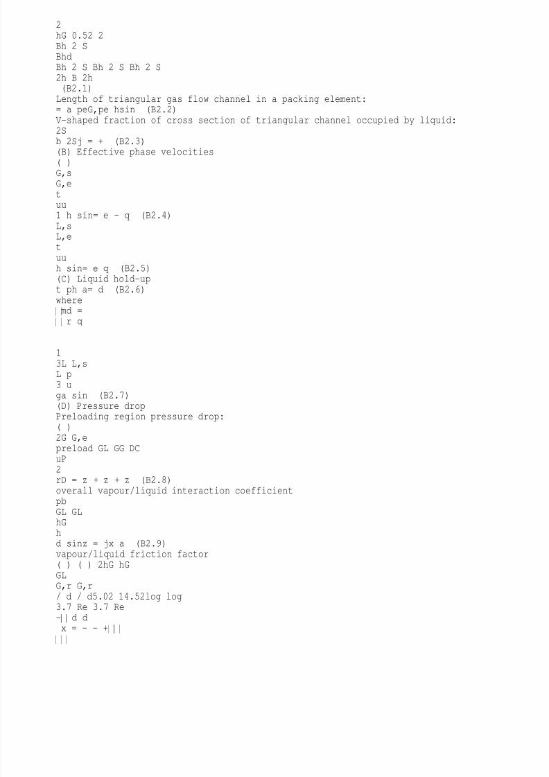
8/10/2019 Erasmus Mass 2004.PDF
http://slidepdf.com/reader/full/erasmus-mass-2004pdf 225/257
2hG 0.52 2Bh 2 SBhdBh 2 S Bh 2 S Bh 2 S2h B 2h (B2.1)Length of triangular gas flow channel in a packing element:= a peG,pe hsin (B2.2)V-shaped fraction of cross section of triangular channel occupied by liquid:2Sb 2Sj = + (B2.3)(B) Effective phase velocities( )G,sG,etuu1 h sin= e - q (B2.4)L,sL,etuu
h sin= e q (B2.5)(C) Liquid hold-upt ph a= d (B2.6)where
md = r q
13L L,sL p3 uga sin (B2.7)
(D) Pressure dropPreloading region pressure drop:( )2G G,epreload GL GG DCuP2rD = z + z + z (B2.8)overall vapour/liquid interaction coefficientpbGL GLhGh
d sinz = jx a (B2.9)vapour/liquid friction factor( ) ( ) 2hG hGGLG,r G,r/ d / d5.02 14.52log log3.7 Re 3.7 Re- d d x = - - +

8/10/2019 Erasmus Mass 2004.PDF
http://slidepdf.com/reader/full/erasmus-mass-2004pdf 226/257
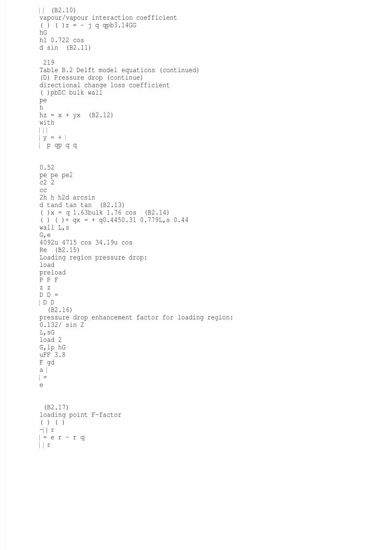
8/10/2019 Erasmus Mass 2004.PDF
http://slidepdf.com/reader/full/erasmus-mass-2004pdf 227/257
(B2.10)vapour/vapour interaction coefficient( ) ( )z = - j q qpb3.14GGhGh1 0.722 cosd sin (B2.11)
219Table B.2 Delft model equations (continued)(D) Pressure drop (continue)directional change loss coefficient( )pbDC bulk wallpehhz = x + yx (B2.12)with
y = + p qp q q
0.52pe pe pe2c2 2
cc2h h h2d arcsind tand tan tan (B2.13)( )x = q 1.63bulk 1.76 cos (B2.14)( ) ( )+ qx = + q0.4450.31 0.779L,s 0.44wall L,sG,e4092u 4715 cos 34.19u cosRe (B2.15)Loading region pressure drop:loadpreloadP P F
z zD D = D D
(B2.16)pressure drop enhancement factor for loading region:0.132/ sin 2L,sGload 2G,lp hGuFF 3.8F gda
=
e
(B2.17)loading point F-factor( ) ( )- r
= e r - r q r

8/10/2019 Erasmus Mass 2004.PDF
http://slidepdf.com/reader/full/erasmus-mass-2004pdf 228/257
0.50.251.15L,s2 LG,lp hG L GG,s GuF 0.053 gd sinu (B2.18)(E) Mass transfer coefficients and effective surface areaVapour phase:2 2G G,lam G,turbk k k= + (B2.19)withG,lam hG 1/ 3 hGG G,rG G,pek d d0.664Sc ReD l= (B2.20)( )x j
= + x j
+ -

8/10/2019 Erasmus Mass 2004.PDF
http://slidepdf.com/reader/full/erasmus-mass-2004pdf 229/257
GL 2 / 3G,r GG,turb hG hGG G,pe2 / 3GLGRe Sck d d81D1 12.7 Sc 18 (B2.21)Liquid phase:L L,eLhGD uk 20.9d= p (B2.22)
220Table B.2 Delft model equations (continued)(E) Mass transfer coefficients and effective surface area (cont.)Effective surface area:( )( )e p
BLs1a aA1u- W=
+
(B2.23)with 6A 2.143 10 , B 1.5-= · = for Montzpak B1-250 (B2.24)(F) Dimensionless groups
( )G,e L,e hG GG,rGu u dRe + r=m (B2.25)GGg GSc Dm= r (B2.26)
Table B.3 Billet model equations(A) Hydraulic diameter and related parametersParticle diameter (used as hydraulic diameter for vapour phase in pressure dropcalculations):
- e=pp1d 6a (B3.1)Hydraulic diameter in mass transfer correlations:- e=pp1d 6
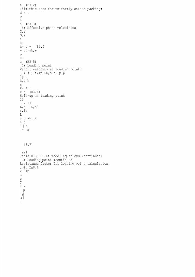
8/10/2019 Erasmus Mass 2004.PDF
http://slidepdf.com/reader/full/erasmus-mass-2004pdf 230/257
a (B3.2)Film thickness for uniformly wetted packing:d = tpha (B3.3)(B) Effective phase velocitiesG,sG,etuuh= e - (B3.4)= dL,sL,epuua (B3.5)(C) Loading pointVapour velocity at loading point:( ) ( ) t,lp LG,s t,lplplp Ghgu har= e -x r (B3.6)
Hold-up at loading point111 2 33L,s L L,s3t,lpLu u ah 12a g- r
= m
(B3.7)
221Table B.3 Billet model equations (continued)(C) Loading point (continued)Resistance factor for loading point calculation:lplp 2n0.42 LlpGgCx =
m
y m

8/10/2019 Erasmus Mass 2004.PDF
http://slidepdf.com/reader/full/erasmus-mass-2004pdf 231/257
(B3.8)Clp is packing specific and:lplp0.4 n 0.3260.4 n 0.723y £ fi = -y > fi = - (B3.9)and with the flow parameter defined as:GLLGry =r (B3.10)(D) Flood pointVapour velocity at flood point:( ) ( )e - r= x re32t,fp t,fp LG,s 1fpfp p G2
h h2gu a (B3.11)Liquid velocity at flood point:( ) ( ) e -r = - m e
t,fp3LL,s t,fp2fpLphg 1 3u h 13 2a (B3.12)
Hold-up at flood point:[ ])ms/(kg4101L05.0WWLLfp,t 3741.0h -·>m
m
rrme= (B3.13)Resistance factor for flood point calculation:fpfp 2n0.22 LfpGgCx =

8/10/2019 Erasmus Mass 2004.PDF
http://slidepdf.com/reader/full/erasmus-mass-2004pdf 232/257
m y m

8/10/2019 Erasmus Mass 2004.PDF
http://slidepdf.com/reader/full/erasmus-mass-2004pdf 233/257
(B3.14)Cfp is packing specific and:fpfp0.4 n 0.1940.4 n 0.708y £ fi = -y > fi = - (B3.15)(E) Pressure dropPressure drop for dry bed:2G,sd d G s3uP a fz 2D = x rD e (B3.16)
222Table B.3 Billet model equations (continued)(E) Pressure drop (continued)Resistance factor for dry bedd p 0.08
G G64 1.8CRe Re
x = +
(B3.17)with the `wall factor' calculated from:s c1 41f ad= + (B3.18)Pressure drop for wet bed:
3wd d tPP h
xD e= D x e -
(B3.19)Resistance factor for wet bed:( )- e -
x = + e
3 xtw p0.08G,s G,sh64 1.8C WRe Re (B3.20)with( )r=- e m

8/10/2019 Erasmus Mass 2004.PDF
http://slidepdf.com/reader/full/erasmus-mass-2004pdf 234/257
G,s p GG,s sGu dRe f1 (B3.21)and
=
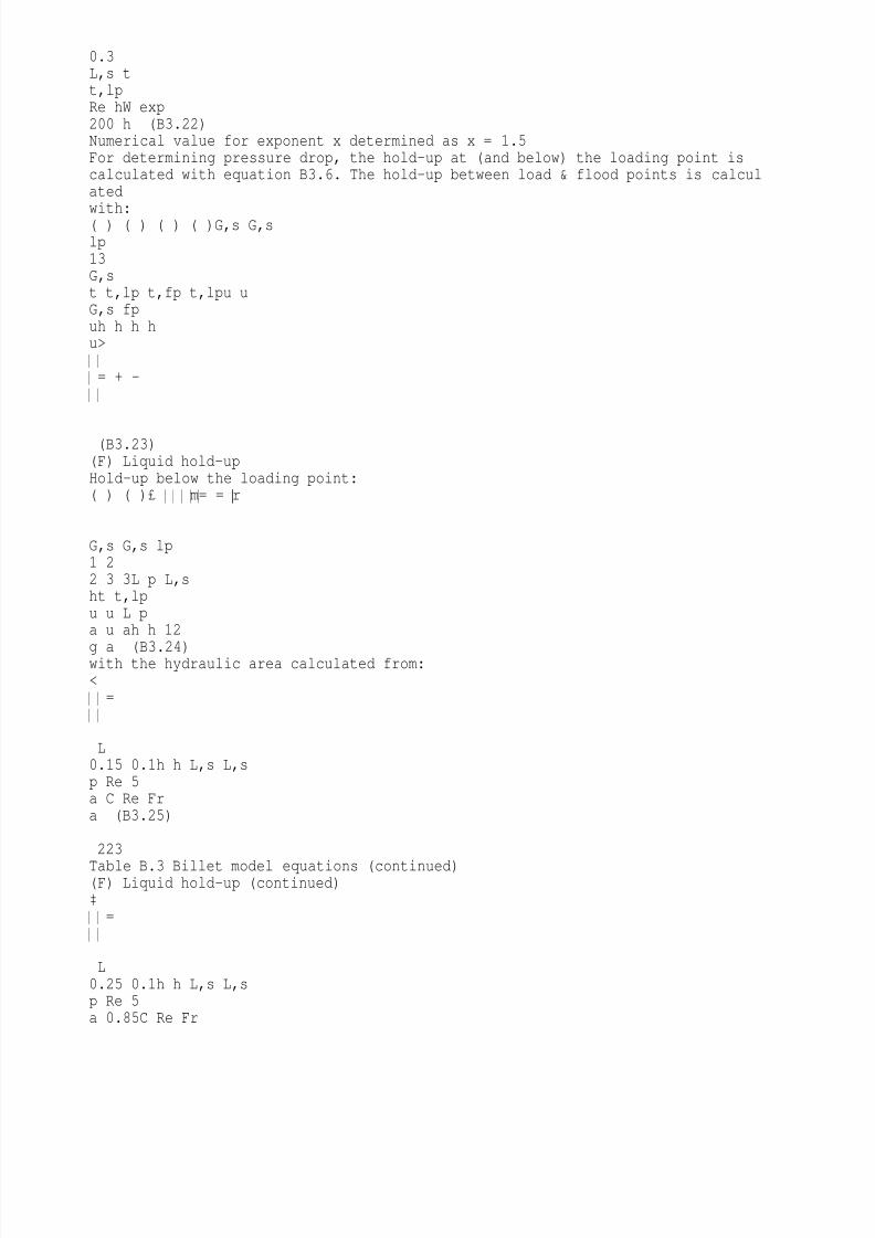
8/10/2019 Erasmus Mass 2004.PDF
http://slidepdf.com/reader/full/erasmus-mass-2004pdf 235/257
0.3L,s tt,lpRe hW exp200 h (B3.22)Numerical value for exponent x determined as x = 1.5For determining pressure drop, the hold-up at (and below) the loading point iscalculated with equation B3.6. The hold-up between load & flood points is calculatedwith:( ) ( ) ( ) ( )G,s G,slp13G,st t,lp t,fp t,lpu uG,s fpuh h h hu>
= + -
(B3.23)(F) Liquid hold-upHold-up below the loading point:( ) ( )£ m = = r
G,s G,s lp1 22 3 3L p L,sht t,lpu u L pa u ah h 12
g a (B3.24)with the hydraulic area calculated from:<
=
L0.15 0.1h h L,s L,sp Re 5a C Re Fra (B3.25)
223
Table B.3 Billet model equations (continued)(F) Liquid hold-up (continued)³
=
L0.25 0.1h h L,s L,sp Re 5a 0.85C Re Fr
8/10/2019 Erasmus Mass 2004.PDF
http://slidepdf.com/reader/full/erasmus-mass-2004pdf 236/257

8/10/2019 Erasmus Mass 2004.PDF
http://slidepdf.com/reader/full/erasmus-mass-2004pdf 237/257
G,s G,s lp13G,se e e ep p p p G,su u lp fp lp fpua a a aa a a a u (B3.32)Effective interfacial area at flood point:
s= s
0.56e eLp W pfp lpa a7a a (B3.33)effective interfacial area for negative surface tension gradient systems:( )- = -
0.54e e
Lp pnega a1 2.4 10 Maa a (B3.34)whereD=mL L L pxMaD a (B3.35)Dx is concentration difference between bulk liquid and surface liquid224Table B.3 Billet model equations (continued)(H) Dimensionless numbers
r=mG,s GG,sp GuRea (B3.36)r=mL,s LL,sp LuRe
a (B3.37)r=s2L,s LL,sL puW ea (B3.38)=2L,s p

8/10/2019 Erasmus Mass 2004.PDF
http://slidepdf.com/reader/full/erasmus-mass-2004pdf 238/257
L,su aFrg (B3.39)GGG GSc Dm= r (B3.40)
225APPENDIX CExperimental data for Flexipac 350YThe experimental pressure drop and hold-up data for Flexipac 350Y for the air/watersystem are given in Figures C.1 and C.2. The experimental data for the air/Kerosol200 system are given in Figures C.3 and C.4. The experimental data are given intable format for the two test systems in Table C.1 and C.2. The dry pressure dropdata are included in Table C.1.Experimental data for Flexipac 350Y HCThe experimental pressure drop and hold-up data for Flexipac 350Y HC for theair/water system are given in Figures C.5 and C.6. The experimental data for the air/Kerosol 200 system are given in Figures C.7 and C.8. The experimental data are
given in table format for the two test systems in Table C.3 and C.4. The dry pressuredrop experimental data are included in Table C.3.
226
Figure C.1 Pressure drop as function of F-factor for Flexipac 350Y, air/watersystem00.020.040.060.08
0.10.120.140.160 0.5 1 1.5 2 2.5 3 3.5 4FG [m/s.(kg/m3)0.5)]ht6.0 12.9 20.5 28.8 35.6uL,s [m3/(m2.hr)]hth
t Figure C.2 Holdup as function of F-factor for Flexipac 350Y, air/water system
0100200300400500

8/10/2019 Erasmus Mass 2004.PDF
http://slidepdf.com/reader/full/erasmus-mass-2004pdf 239/257
600700800900100011000 0.5 1 1.5 2 2.5 3 3.5 4 4.5FG [m/s.(kg/m3)0.5)]dP/dz [Pa/m]0.0 6.0 12.920.5 28.8 35.6uL,s [m3/(m2.hr)]227
Figure C.3 Pressure drop as function of F-factor for Flexipac 350Y, air/Kerosol200 system00.020.040.060.080.10.120.140.160 0.5 1 1.5 2 2.5 3 3.5
FG [m/s.(kg/m3)0.5)]ht6.1 12.7 20.6 28.8 35.6uL,s [m3/(m2.hr)]htht Figure C.4 Holdup as function of F-factor for Flexipac 350Y, air/Kerosol 200system
0100200300400500600700800900

8/10/2019 Erasmus Mass 2004.PDF
http://slidepdf.com/reader/full/erasmus-mass-2004pdf 240/257
100011000 0.5 1 1.5 2 2.5 3 3.5FG [m/s.(kg/m3)0.5)]dP/dz [Pa/m]0.0 6.1 12.720.6 28.8 35.6uL,s [m3/(m2.hr)]228
Figure C.5 Pressure drop as function of F-factor for Flexipac 350Y HC, air/water system
00.020.040.060.080.10.120.140.160.180 0.5 1 1.5 2 2.5 3 3.5 4 4.5FG [m/s.(kg/m3)0.5)]h
t6.0 12.8 20.5 28.8 35.7uL,s [m3/(m2.hr)]htht Figure C.6 Holdup as function of F-factor for Flexipac 350Y HC, air/water system 0100200
300400500600700800900100011001200
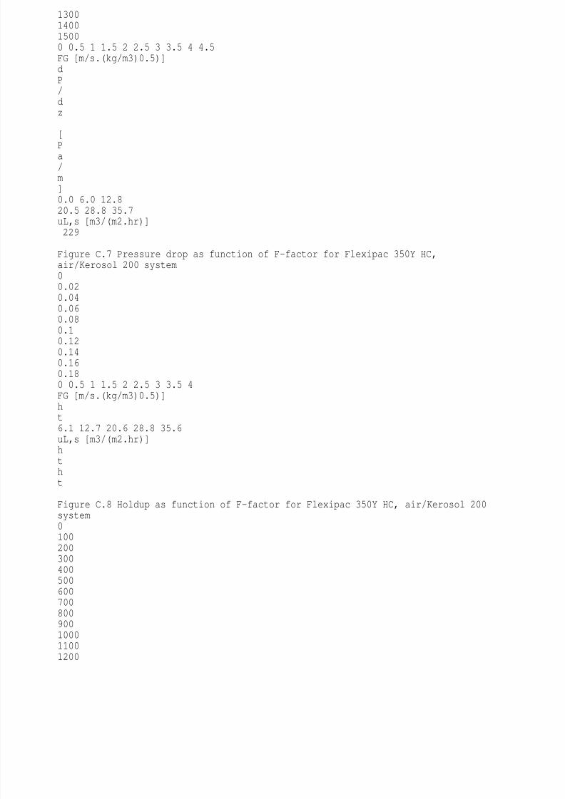
8/10/2019 Erasmus Mass 2004.PDF
http://slidepdf.com/reader/full/erasmus-mass-2004pdf 241/257
1300140015000 0.5 1 1.5 2 2.5 3 3.5 4 4.5FG [m/s.(kg/m3)0.5)]dP/dz [Pa/m]0.0 6.0 12.820.5 28.8 35.7uL,s [m3/(m2.hr)]229
Figure C.7 Pressure drop as function of F-factor for Flexipac 350Y HC,air/Kerosol 200 system
00.020.040.060.080.10.120.140.160.180 0.5 1 1.5 2 2.5 3 3.5 4FG [m/s.(kg/m3)0.5)]h
t6.1 12.7 20.6 28.8 35.6uL,s [m3/(m2.hr)]htht Figure C.8 Holdup as function of F-factor for Flexipac 350Y HC, air/Kerosol 200system0100200
300400500600700800900100011001200

8/10/2019 Erasmus Mass 2004.PDF
http://slidepdf.com/reader/full/erasmus-mass-2004pdf 242/257
0 0.5 1 1.5 2 2.5 3 3.5 4 4.5FG [m/s.(kg/m3)0.5)]dP/dz [Pa/m]0.0 6.1 12.720.6 28.8 35.6uL,s [m3/(m2.hr)]230
Table C.1 Experimental data for Flexipac 350Y, air/water systemT1 T2 T3 T4 Pt uG,s F dP/dz ht[oC] [oC] [oC] [oC] [mmHg] [m/s] [(Pa)0.5] [Pa/m] [m3/m3]uL,s = 35.6 [m3/(m2.hr)]n/a n/a 25.3 25.4 n/a 0 0 0 0.090
n/a n/a 25.7 25.8 n/a 0 0 0 0.09229.4 25.2 25.4 25.2 752 0.80 0.87 43 0.09030 25.2 25.5 24.8 752 0.81 0.87 44 0.08930.4 25 25.2 24.7 748 1.09 1.18 88 0.09230 25 25.2 24.7 748 1.10 1.18 91 0.08929.1 25 25.2 24.6 749 1.38 1.49 138 0.09229.1 24.9 25.2 24.3 749 1.38 1.50 136 0.09128.5 25 25.5 24.6 753.5 1.61 1.75 208 0.10024.7 23.3 23.6 22.4 754 1.75 1.90 248 0.08826 23.7 24 22.6 754 1.75 1.91 247 0.08629.5 23.5 23.5 23.2 753.5 1.76 1.91 245 0.10327.8 24.7 25.1 24.2 754 1.79 1.94 277 0.09830.6 25.1 25.3 24.7 752 1.98 2.14 365 0.108
30.9 24.7 24.7 24.2 752 1.98 2.14 390 0.10630.1 24.2 24.8 23.6 753 1.98 2.15 409 0.10729.5 25.5 25.7 24.4 753.5 2.04 2.21 541 0.11430 25 25.4 24.2 752 2.06 2.23 881 0.12931 25.1 25.1 24.4 752 2.13 2.30 717 0.12530.7 25.1 25.3 24.4 752 2.13 2.31 667 0.12426.4 24.2 24.5 22.7 754 2.16 2.35 780 0.11326.9 23.9 24 22.4 754 2.17 2.36 752 0.109uL,s = 28.8 [m3/(m2.hr)]n/a n/a 25.6 25.5 n/a 0 0 0 0.093n/a n/a 26 25.9 n/a 0 0 0 0.09126 25.5 25.8 25.5 752.5 0.80 0.87 42 0.08730.2 25.4 25.5 24.8 752 0.81 0.87 42 0.087
28.5 25 25.2 24.7 748 1.09 1.18 86 0.08925.8 24.6 25.3 24 752.5 1.09 1.18 87 0.08427.6 24.9 25.3 24.4 752.5 1.09 1.18 86 0.08529.6 25.1 25.1 24.4 749 1.39 1.50 146 0.08929.8 25 25.2 24.2 749 1.39 1.50 142 0.09129.3 24.5 25 23.9 753 1.70 1.84 204 0.09427.7 24.2 24.4 23 753.5 1.75 1.90 221 0.07827.8 24.2 24.4 23.3 753.5 1.75 1.90 220 0.07929.5 25 25.1 24.1 753.5 1.85 2.00 252 0.09727.8 24.8 25.2 23.7 754 1.87 2.02 252 0.092
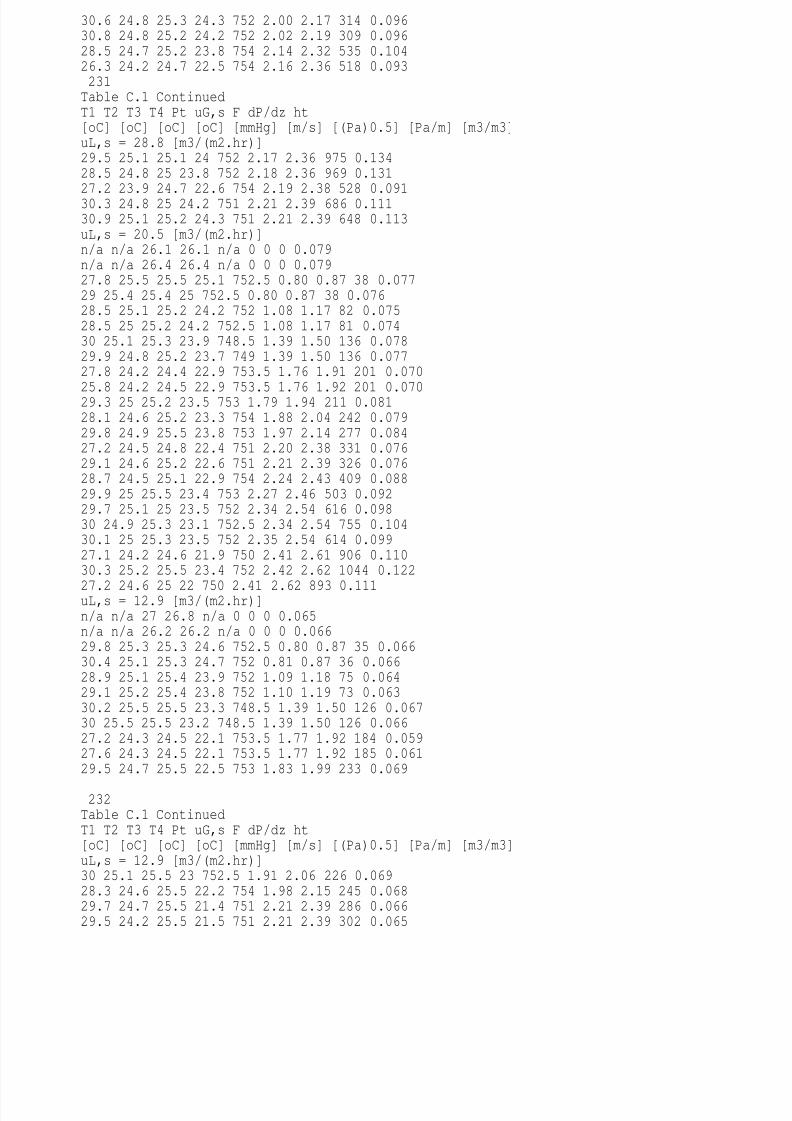
8/10/2019 Erasmus Mass 2004.PDF
http://slidepdf.com/reader/full/erasmus-mass-2004pdf 243/257
30.6 24.8 25.3 24.3 752 2.00 2.17 314 0.09630.8 24.8 25.2 24.2 752 2.02 2.19 309 0.09628.5 24.7 25.2 23.8 754 2.14 2.32 535 0.10426.3 24.2 24.7 22.5 754 2.16 2.36 518 0.093231Table C.1 ContinuedT1 T2 T3 T4 Pt uG,s F dP/dz ht[oC] [oC] [oC] [oC] [mmHg] [m/s] [(Pa)0.5] [Pa/m] [m3/m3]uL,s = 28.8 [m3/(m2.hr)]29.5 25.1 25.1 24 752 2.17 2.36 975 0.13428.5 24.8 25 23.8 752 2.18 2.36 969 0.13127.2 23.9 24.7 22.6 754 2.19 2.38 528 0.09130.3 24.8 25 24.2 751 2.21 2.39 686 0.11130.9 25.1 25.2 24.3 751 2.21 2.39 648 0.113uL,s = 20.5 [m3/(m2.hr)]n/a n/a 26.1 26.1 n/a 0 0 0 0.079n/a n/a 26.4 26.4 n/a 0 0 0 0.07927.8 25.5 25.5 25.1 752.5 0.80 0.87 38 0.07729 25.4 25.4 25 752.5 0.80 0.87 38 0.07628.5 25.1 25.2 24.2 752 1.08 1.17 82 0.07528.5 25 25.2 24.2 752.5 1.08 1.17 81 0.07430 25.1 25.3 23.9 748.5 1.39 1.50 136 0.07829.9 24.8 25.2 23.7 749 1.39 1.50 136 0.07727.8 24.2 24.4 22.9 753.5 1.76 1.91 201 0.070
25.8 24.2 24.5 22.9 753.5 1.76 1.92 201 0.07029.3 25 25.2 23.5 753 1.79 1.94 211 0.08128.1 24.6 25.2 23.3 754 1.88 2.04 242 0.07929.8 24.9 25.5 23.8 753 1.97 2.14 277 0.08427.2 24.5 24.8 22.4 751 2.20 2.38 331 0.07629.1 24.6 25.2 22.6 751 2.21 2.39 326 0.07628.7 24.5 25.1 22.9 754 2.24 2.43 409 0.08829.9 25 25.5 23.4 753 2.27 2.46 503 0.09229.7 25.1 25 23.5 752 2.34 2.54 616 0.09830 24.9 25.3 23.1 752.5 2.34 2.54 755 0.10430.1 25 25.3 23.5 752 2.35 2.54 614 0.09927.1 24.2 24.6 21.9 750 2.41 2.61 906 0.11030.3 25.2 25.5 23.4 752 2.42 2.62 1044 0.122
27.2 24.6 25 22 750 2.41 2.62 893 0.111uL,s = 12.9 [m3/(m2.hr)]n/a n/a 27 26.8 n/a 0 0 0 0.065n/a n/a 26.2 26.2 n/a 0 0 0 0.06629.8 25.3 25.3 24.6 752.5 0.80 0.87 35 0.06630.4 25.1 25.3 24.7 752 0.81 0.87 36 0.06628.9 25.1 25.4 23.9 752 1.09 1.18 75 0.06429.1 25.2 25.4 23.8 752 1.10 1.19 73 0.06330.2 25.5 25.5 23.3 748.5 1.39 1.50 126 0.06730 25.5 25.5 23.2 748.5 1.39 1.50 126 0.06627.2 24.3 24.5 22.1 753.5 1.77 1.92 184 0.05927.6 24.3 24.5 22.1 753.5 1.77 1.92 185 0.06129.5 24.7 25.5 22.5 753 1.83 1.99 233 0.069
232Table C.1 ContinuedT1 T2 T3 T4 Pt uG,s F dP/dz ht[oC] [oC] [oC] [oC] [mmHg] [m/s] [(Pa)0.5] [Pa/m] [m3/m3]uL,s = 12.9 [m3/(m2.hr)]30 25.1 25.5 23 752.5 1.91 2.06 226 0.06928.3 24.6 25.5 22.2 754 1.98 2.15 245 0.06829.7 24.7 25.5 21.4 751 2.21 2.39 286 0.06629.5 24.2 25.5 21.5 751 2.21 2.39 302 0.065

8/10/2019 Erasmus Mass 2004.PDF
http://slidepdf.com/reader/full/erasmus-mass-2004pdf 244/257
28 24.5 25.2 20.8 750 2.42 2.62 440 0.07327.8 24.3 25.3 20.7 750 2.42 2.62 462 0.07431.3 25 25.6 22.6 752 2.55 2.76 616 0.08531.2 25 25.5 22.8 752 2.56 2.77 616 0.08530 24.6 25.7 22.3 752 2.64 2.86 881 0.09728.5 24 25.2 20.8 749.5 2.65 2.87 742 0.08828.4 24.4 25.5 20.6 749.5 2.65 2.88 755 0.090uL,s = 6.0 [m3/(m2.hr)]n/a n/a 27 26.6 n/a 0 0 0 0.051n/a n/a 27.3 26.6 n/a 0 0 0 0.05129.4 26.5 26.8 24.6 752 0.80 0.87 34 0.05030.1 26.8 27 24.3 752 0.81 0.87 33 0.05129.5 25.8 26.5 22.9 752 1.10 1.19 67 0.05129.5 25.6 26.1 22.8 752 1.10 1.19 68 0.05130.2 25.1 26 21.2 748.5 1.39 1.50 116 0.05130 25.1 25.8 21.2 748.5 1.39 1.51 117 0.05126 23.9 25.7 20.3 753.5 1.76 1.92 164 0.04827.5 23.4 25.8 20 753.5 1.77 1.92 166 0.04629.8 23.4 25.5 19.7 751 2.21 2.39 273 0.05329.9 23.4 25.5 19.6 751 2.21 2.39 274 0.05228.3 22.8 25.8 19.2 750 2.47 2.68 371 0.05328.1 22.9 26.2 19 750 2.47 2.68 355 0.05529.1 22.8 26 19.5 749.5 2.77 3.01 503 0.06029.1 22.5 25.7 19.2 749.5 2.77 3.01 509 0.058
29.9 23 25.8 20.7 752 3.00 3.25 686 0.07029.5 22.9 25.5 20.4 752 3.10 3.36 950 0.081uL,s = 0.0 [m3/(m2.hr)]23.5 21.7 n/a n/a 753.5 0.77 0.84 8 027.1 25 n/a n/a 753.5 1.09 1.19 38 027.2 25.6 n/a n/a 753.5 1.40 1.53 72 027.5 26 n/a n/a 753.5 1.79 1.94 112 026.8 25.4 n/a n/a 754 2.17 2.35 146 027.6 26.6 n/a n/a 753.5 2.18 2.36 171 027.6 26.8 n/a n/a 753.5 2.51 2.73 223 027.2 26.8 n/a n/a 753.5 2.77 3.01 272 026.2 24.6 n/a n/a 754 2.78 3.02 252 025.6 23.9 n/a n/a 754 3.22 3.50 347 0
25.6 23.7 n/a n/a 754 3.55 3.88 416 0233Table C.2 Experimental data for Flexipac 350Y, air/Kerosol 200 systemT1 T2 T3 T4 Pt uG,s F dP/dz ht[oC] [oC] [oC] [oC] [mmHg] [m/s] [(Pa)0.5] [Pa/m] [m3/m3]uL,s = 35.6 [m3/(m2.hr)]n/a n/a 31.6 31.4 n/a 0 0 0 0.11129.5 30 30.9 30.5 751.5 1.02 1.10 107 0.10829.1 31.4 32 31.4 751.5 1.35 1.46 189 0.11227.5 29.9 30.3 29.7 754.5 1.58 1.71 325 0.12032.1 31.1 31.2 31.1 753 1.68 1.80 371 0.12232.0 31.4 31.6 31.4 753 1.75 1.88 491 0.12831.6 31.4 31.7 31.4 753 1.82 1.95 642 0.138
30.6 31 31 30.9 753 1.84 1.98 818 0.153uL,s = 28.8 [m3/(m2.hr)]n/a n/a 31.2 31 n/a 0 0 0 0.09730.0 30.7 31.3 31.3 751.5 1.00 1.08 88 0.09529.8 30.6 31.2 30.8 751.5 1.35 1.45 151 0.09830.0 30.8 31.7 31 757 1.66 1.79 245 0.10132.0 31.1 31.6 31.5 753 1.82 1.96 350 0.10532.1 30.8 31.6 31.5 753 1.90 2.04 484 0.11332.1 31.1 31.4 31.5 753 1.93 2.08 610 0.12232.0 31.1 31.4 31.4 753 1.97 2.12 755 0.134

8/10/2019 Erasmus Mass 2004.PDF
http://slidepdf.com/reader/full/erasmus-mass-2004pdf 245/257
31.7 30.8 31.3 31.3 753 2.02 2.18 893 0.144uL,s = 20.6 [m3/(m2.hr)]n/a n/a 31.4 31.3 n/a 0 0 0 0.07730.6 30.6 31.4 31.1 751.5 1.09 1.17 82 0.08129.4 30.3 30.9 30.4 756 1.54 1.67 161 0.08529.3 30.2 30.8 30.2 756 1.87 2.02 258 0.08829.8 30.6 31 30.5 756.5 2.02 2.19 358 0.09429.7 30.2 31.2 30.2 756.5 2.09 2.26 509 0.10429.5 30.2 30.9 30.2 756.5 2.11 2.29 614 0.11329.1 30.2 31 30 756.5 2.17 2.35 767 0.12229.1 30 30.8 29.9 757 2.21 2.40 956 0.136uL,s = 12.7 [m3/(m2.hr)]n/a n/a 31.7 31.1 n/a 0 0 0 0.06030.5 30.7 31.3 30.6 751.5 1.14 1.23 75 0.06530.3 31.4 32.1 31.1 751.5 1.39 1.50 123 0.06627.8 29.9 30.8 29.3 754.5 1.76 1.90 201 0.06829.1 30.4 31.3 29.7 752.5 2.02 2.18 264 0.07228.8 30.6 31.6 30 752.5 2.25 2.43 384 0.07929.9 30.6 31.2 30 756 2.32 2.51 509 0.08729.8 30.6 31.3 30 756 2.37 2.56 629 0.09629.5 30.6 31.2 29.8 756 2.41 2.61 767 0.10629.0 30 30.9 29.3 756 2.48 2.69 887 0.115
234
Table C.2 ContinuedT1 T2 T3 T4 Pt uG,s F dP/dz ht[oC] [oC] [oC] [oC] [mmHg] [m/s] [(Pa)0.5] [Pa/m] [m3/m3]uL,s = 6.1 [m3/(m2.hr)]n/a n/a 31.7 30.5 n/a 0 0 0 0.04530.4 30.3 32 30.1 751 1.12 1.21 63 0.04630.4 31.2 31.9 30.4 751.5 1.37 1.48 107 0.04628.1 30.4 31.3 28.4 754.5 1.63 1.76 151 0.04830.2 31.9 33 30.4 751.5 1.98 2.13 211 0.05129.8 31.2 32.5 29.7 752 2.34 2.52 333 0.05529.4 31 32.7 29.2 752 2.55 2.75 459 0.06329.0 30.9 32.9 29.2 752 2.67 2.89 579 0.07030.2 31.2 33 30 751.5 2.84 3.06 711 0.079
30.2 30.3 31.3 30 751.5 2.98 3.21 912 0.095
Table C.3 Experimental data for Flexipac 350Y HC, air/water systemT1 T2 T3 T4 Pt uG,s F dP/dz ht[oC] [oC] [oC] [oC] [mmHg] [m/s] [(Pa)0.5] [Pa/m] [m3/m3]uL,s = 35.7 [m3/(m2.hr)]n/a n/a 25.9 25.5 754 0 0 0 0.10130 25.1 25.3 24.8 748 1.11 1.19 104 0.10335.1 26.2 26.4 26 746 1.17 1.25 101 0.10335.4 26.4 26.5 26 746 1.37 1.47 157 0.10430.3 24.8 25 24.6 748 1.37 1.48 182 0.10530 25 25.5 24.7 752 1.63 1.76 283 0.11630.2 24.9 25 24.5 752 1.65 1.78 283 0.115
30.6 25.2 25 24.4 747 1.68 1.81 252 0.11929.5 25 25 24.4 751.5 1.98 2.14 371 0.11627.2 24.7 25 24.3 751.5 2.00 2.17 371 0.11528.1 24.5 24.8 23 755 2.14 2.32 478 0.12230.2 24.9 25 24.4 751.5 2.30 2.49 604 0.12430.1 25.1 25.1 24.4 751.5 2.31 2.51 610 0.12830.2 25 25 24.5 751.5 2.37 2.57 692 0.13027.4 24.7 25 24 751.5 2.37 2.57 704 0.13027 24.1 24.4 22.8 754 2.49 2.71 881 0.13729.9 24.7 25 24.3 751.5 2.51 2.72 868 0.123

8/10/2019 Erasmus Mass 2004.PDF
http://slidepdf.com/reader/full/erasmus-mass-2004pdf 246/257
32.4 25 25 24.4 748.5 2.54 2.74 1321 0.16530.3 25 25 24.3 748.5 2.57 2.77 1006 0.145uL,s = 28.8 [m3/(m2.hr)]n/a n/a 25.5 25.5 754 0 0 0 0.10130.6 25.1 25.2 24.7 748 1.06 1.15 91 0.10534.7 26.3 26.4 25.9 746 1.16 1.25 98 0.10734.4 26.2 26.1 25.7 746 1.37 1.47 148 0.10730 24.6 25 24.2 748 1.37 1.48 164 0.108
235Table C.3 ContinuedT1 T2 T3 T4 Pt uG,s F dP/dz ht[oC] [oC] [oC] [oC] [mmHg] [m/s] [(Pa)0.5] [Pa/m] [m3/m3]uL,s = 28.8 [m3/(m2.hr)]27.2 24.5 25 23.2 755.5 1.70 1.85 260 0.11127 24.6 25 23.3 755.5 1.71 1.86 258 0.11126.8 24.2 24.3 22.5 755.5 1.99 2.16 365 0.11327 24 24.4 22.6 755 2.01 2.18 369 0.11326.9 23.9 24 22.4 755.5 2.19 2.38 468 0.11927.5 23.8 24 22.3 755.5 2.21 2.40 465 0.11823.3 24 24 21.9 755 2.28 2.49 981 0.11926 23.8 24 21.8 755 2.33 2.54 597 0.11929.8 25 25 23.8 752 2.49 2.70 836 0.12729.1 24.6 25 23.4 752 2.50 2.71 849 0.132
26.9 24.2 24.4 22.1 754 2.56 2.78 792 0.12533 25 25 24.1 747.5 2.67 2.88 1358 0.15433.2 25 25.1 24.1 748 2.70 2.91 1038 0.138uL,s = 20.5 [m3/(m2.hr)]n/a n/a 25.6 25.4 754 0 0 0 0.08834.5 25.9 25.8 25.5 746 1.11 1.19 81 0.09134.3 25.9 25.7 25 746 1.38 1.48 141 0.09228.2 24.7 25.1 22.5 756 1.76 1.91 249 0.09828 25 25 22.4 756 1.77 1.92 249 0.09727.8 24.4 24.6 21.9 756 2.11 2.30 377 0.10028.1 24.6 25 21.7 756 2.12 2.31 375 0.10126.7 24.2 24.4 21.4 756 2.37 2.58 509 0.10627.2 24.3 24.6 21.3 756 2.39 2.60 528 0.106
26.6 23.8 24 20.8 756 2.65 2.89 723 0.11324.9 24.2 24.4 20.8 756 2.65 2.89 717 0.11225.1 24.5 25 21.4 754 2.80 3.05 855 0.11827.3 23.7 24 21 754 2.88 3.14 987 0.12133 25 25 23.5 747.5 2.97 3.20 1245 0.131uL,s = 12.8 [m3/(m2.hr)]n/a n/a 25.4 25 754 0 0 0 0.07530.7 25.4 25.5 24.2 748 1.06 1.14 78 0.07830.8 25.2 25.2 23.8 748 1.38 1.49 145 0.08028.5 25 25.1 21.4 755 1.82 1.97 249 0.08428.5 24.3 24.7 20.5 755.5 2.21 2.40 387 0.08928 24.2 24.7 19.8 755.5 2.46 2.68 491 0.09127.6 23.8 24.8 19.3 755.5 2.70 2.95 629 0.095
27.2 23.4 25.2 19.4 755.5 2.71 2.96 642 0.09426.6 23.9 25 19.9 752.5 2.86 3.11 755 0.10127.6 23.7 24.7 19.8 752.5 3.03 3.29 906 0.103
236Table C.3 ContinuedT1 T2 T3 T4 Pt uG,s F dP/dz ht[oC] [oC] [oC] [oC] [mmHg] [m/s] [(Pa)0.5] [Pa/m] [m3/m3]uL,s = 12.8 [m3/(m2.hr)]27.8 23.7 24.9 19.8 752.5 3.10 3.37 994 0.105

8/10/2019 Erasmus Mass 2004.PDF
http://slidepdf.com/reader/full/erasmus-mass-2004pdf 247/257
33.1 25.1 25.3 23.2 746 3.24 3.49 1075 0.10930.8 24.6 25.6 21.7 747 3.38 3.65 1170 0.11130.6 24.8 25.5 22.1 748 3.46 3.74 1403 0.124uL,s = 6.0 [m3/(m2.hr)]n/a n/a 26 26 754 0 0 0 0.06030.8 25.4 25.8 22.8 748 1.13 1.22 82 0.06330.6 24.5 25 22.5 748 1.38 1.49 132 0.06428.5 23.6 26 18.3 755 1.93 2.10 254 0.06728.4 22.5 26.4 17.9 755 2.37 2.57 387 0.06927.7 22 25.3 17.6 755 2.75 3.00 543 0.07428.1 22.3 26.5 18.5 752.5 2.99 3.25 679 0.07828.1 21.8 26.1 18.2 752.5 3.17 3.45 818 0.08427.8 21.7 26.5 18.1 752.5 3.32 3.62 925 0.08530.2 23 25.8 21 747 3.67 3.97 1006 0.08430.7 23.2 25.7 21.7 747.5 3.75 4.05 1138 0.08930.5 22.9 26 21.4 748 3.82 4.13 1258 0.095uL,s = 0.0 [m3/(m2.hr)]35.4 30.2 n/a n/a 746 1.20 1.29 43 035.2 28.8 n/a n/a 746 1.39 1.49 74 030.7 29.8 n/a n/a 751.5 1.81 1.95 144 030.4 29.6 n/a n/a 751.5 2.19 2.35 209 032.1 31.1 n/a n/a 748.5 2.36 2.53 225 029.8 29.1 n/a n/a 751.5 2.44 2.63 266 030.7 30.2 n/a n/a 751.5 2.60 2.80 310 0
31.6 29.5 n/a n/a 748.5 2.78 2.99 329 028.1 27.6 n/a n/a 751.5 2.84 3.08 364 025 24 n/a n/a 754 2.96 3.22 369 031.3 28.7 n/a n/a 748.5 3.00 3.23 388 031.8 30.8 n/a n/a 748.5 3.10 3.33 417 031 27.7 n/a n/a 748.5 3.37 3.63 490 030.8 24.8 n/a n/a 748.5 3.61 3.90 574 032 30.4 n/a n/a 748.5 3.64 3.92 574 0
237Table C.4 Experimental data for Flexipac 350Y HC, air/Kerosol 200 systemT1 T2 T3 T4 Pt uG,s F dP/dz ht[oC] [oC] [oC] [oC] [mmHg] [m/s] [(Pa)0.5] [Pa/m] [m3/m3]
uL,s = 35.6 [m3/(m2.hr)]n/a n/a 30.9 30.7 n/a 0 0 0 0.11728.4 29.8 30.6 30.2 751.5 0.82 0.88 88 0.11429 30.1 30.8 30.6 752 1.12 1.21 141 0.11828.7 30.6 30.7 30.6 752 1.34 1.44 252 0.12430.2 30.4 31 30.5 751.5 1.55 1.67 346 0.12827.5 30.2 30.8 30.1 751.5 1.65 1.78 421 0.13127.8 30.4 30.8 30 751.5 1.82 1.96 610 0.14127.7 30.2 30.5 30 751.5 1.91 2.06 818 0.15230.8 31.1 31.7 31.2 751 1.94 2.09 912 n/auL,s = 28.8 [m3/(m2.hr)]n/a n/a 31 30.9 n/a 0 0 0 0.10328.5 29.5 30.8 30.4 751.5 0.82 0.88 82 0.103
29.4 30.2 30.9 30.6 752 1.13 1.21 126 0.10529.5 30.6 31 30.9 752 1.37 1.48 201 0.10730 30.7 31 30.8 751.5 1.63 1.75 289 0.11027.2 30.2 30.9 30.1 753 1.76 1.90 384 0.11226.7 30 30.8 29.8 753 1.91 2.06 516 0.11626.2 29.9 30.8 29.6 753 2.01 2.18 654 0.12226.3 30 30.8 29.5 753 2.08 2.25 818 0.13626.3 29.7 30.7 29.5 753 2.13 2.31 1050 0.158uL,s = 20.6 [m3/(m2.hr)]n/a n/a 31.2 31 n/a 0 0 0 0.085
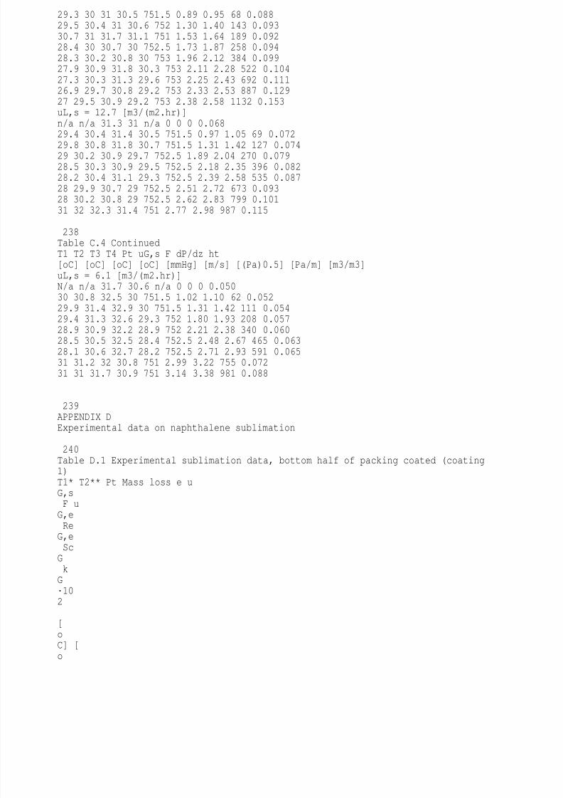
8/10/2019 Erasmus Mass 2004.PDF
http://slidepdf.com/reader/full/erasmus-mass-2004pdf 248/257
29.3 30 31 30.5 751.5 0.89 0.95 68 0.08829.5 30.4 31 30.6 752 1.30 1.40 143 0.09330.7 31 31.7 31.1 751 1.53 1.64 189 0.09228.4 30 30.7 30 752.5 1.73 1.87 258 0.09428.3 30.2 30.8 30 753 1.96 2.12 384 0.09927.9 30.9 31.8 30.3 753 2.11 2.28 522 0.10427.3 30.3 31.3 29.6 753 2.25 2.43 692 0.11126.9 29.7 30.8 29.2 753 2.33 2.53 887 0.12927 29.5 30.9 29.2 753 2.38 2.58 1132 0.153uL,s = 12.7 [m3/(m2.hr)]n/a n/a 31.3 31 n/a 0 0 0 0.06829.4 30.4 31.4 30.5 751.5 0.97 1.05 69 0.07229.8 30.8 31.8 30.7 751.5 1.31 1.42 127 0.07429 30.2 30.9 29.7 752.5 1.89 2.04 270 0.07928.5 30.3 30.9 29.5 752.5 2.18 2.35 396 0.08228.2 30.4 31.1 29.3 752.5 2.39 2.58 535 0.08728 29.9 30.7 29 752.5 2.51 2.72 673 0.09328 30.2 30.8 29 752.5 2.62 2.83 799 0.10131 32 32.3 31.4 751 2.77 2.98 987 0.115
238Table C.4 ContinuedT1 T2 T3 T4 Pt uG,s F dP/dz ht[oC] [oC] [oC] [oC] [mmHg] [m/s] [(Pa)0.5] [Pa/m] [m3/m3]
uL,s = 6.1 [m3/(m2.hr)]N/a n/a 31.7 30.6 n/a 0 0 0 0.05030 30.8 32.5 30 751.5 1.02 1.10 62 0.05229.9 31.4 32.9 30 751.5 1.31 1.42 111 0.05429.4 31.3 32.6 29.3 752 1.80 1.93 208 0.05728.9 30.9 32.2 28.9 752 2.21 2.38 340 0.06028.5 30.5 32.5 28.4 752.5 2.48 2.67 465 0.06328.1 30.6 32.7 28.2 752.5 2.71 2.93 591 0.06531 31.2 32 30.8 751 2.99 3.22 755 0.07231 31 31.7 30.9 751 3.14 3.38 981 0.088
239
APPENDIX DExperimental data on naphthalene sublimation
240Table D.1 Experimental sublimation data, bottom half of packing coated (coating1)T1* T2** Pt Mass loss e uG,s F uG,e ReG,e Sc
G kG·102 [oC] [o
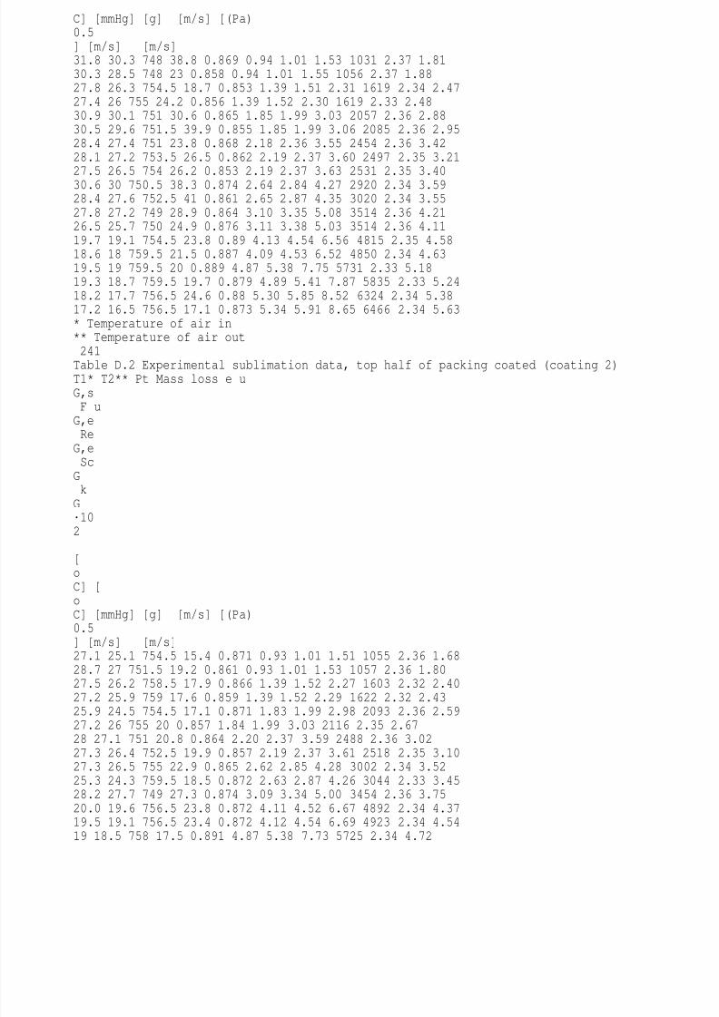
8/10/2019 Erasmus Mass 2004.PDF
http://slidepdf.com/reader/full/erasmus-mass-2004pdf 249/257
C] [mmHg] [g] [m/s] [(Pa)0.5] [m/s] [m/s]31.8 30.3 748 38.8 0.869 0.94 1.01 1.53 1031 2.37 1.8130.3 28.5 748 23 0.858 0.94 1.01 1.55 1056 2.37 1.8827.8 26.3 754.5 18.7 0.853 1.39 1.51 2.31 1619 2.34 2.4727.4 26 755 24.2 0.856 1.39 1.52 2.30 1619 2.33 2.4830.9 30.1 751 30.6 0.865 1.85 1.99 3.03 2057 2.36 2.8830.5 29.6 751.5 39.9 0.855 1.85 1.99 3.06 2085 2.36 2.9528.4 27.4 751 23.8 0.868 2.18 2.36 3.55 2454 2.36 3.4228.1 27.2 753.5 26.5 0.862 2.19 2.37 3.60 2497 2.35 3.2127.5 26.5 754 26.2 0.853 2.19 2.37 3.63 2531 2.35 3.4030.6 30 750.5 38.3 0.874 2.64 2.84 4.27 2920 2.34 3.5928.4 27.6 752.5 41 0.861 2.65 2.87 4.35 3020 2.34 3.5527.8 27.2 749 28.9 0.864 3.10 3.35 5.08 3514 2.36 4.2126.5 25.7 750 24.9 0.876 3.11 3.38 5.03 3514 2.36 4.1119.7 19.1 754.5 23.8 0.89 4.13 4.54 6.56 4815 2.35 4.5818.6 18 759.5 21.5 0.887 4.09 4.53 6.52 4850 2.34 4.6319.5 19 759.5 20 0.889 4.87 5.38 7.75 5731 2.33 5.1819.3 18.7 759.5 19.7 0.879 4.89 5.41 7.87 5835 2.33 5.2418.2 17.7 756.5 24.6 0.88 5.30 5.85 8.52 6324 2.34 5.3817.2 16.5 756.5 17.1 0.873 5.34 5.91 8.65 6466 2.34 5.63* Temperature of air in** Temperature of air out
241Table D.2 Experimental sublimation data, top half of packing coated (coating 2)T1* T2** Pt Mass loss e uG,s F uG,e ReG,e ScG kG·10
2 [oC] [oC] [mmHg] [g] [m/s] [(Pa)0.5] [m/s] [m/s]27.1 25.1 754.5 15.4 0.871 0.93 1.01 1.51 1055 2.36 1.6828.7 27 751.5 19.2 0.861 0.93 1.01 1.53 1057 2.36 1.8027.5 26.2 758.5 17.9 0.866 1.39 1.52 2.27 1603 2.32 2.4027.2 25.9 759 17.6 0.859 1.39 1.52 2.29 1622 2.32 2.43
25.9 24.5 754.5 17.1 0.871 1.83 1.99 2.98 2093 2.36 2.5927.2 26 755 20 0.857 1.84 1.99 3.03 2116 2.35 2.6728 27.1 751 20.8 0.864 2.20 2.37 3.59 2488 2.36 3.0227.3 26.4 752.5 19.9 0.857 2.19 2.37 3.61 2518 2.35 3.1027.3 26.5 755 22.9 0.865 2.62 2.85 4.28 3002 2.34 3.5225.3 24.3 759.5 18.5 0.872 2.63 2.87 4.26 3044 2.33 3.4528.2 27.7 749 27.3 0.874 3.09 3.34 5.00 3454 2.36 3.7520.0 19.6 756.5 23.8 0.872 4.11 4.52 6.67 4892 2.34 4.3719.5 19.1 756.5 23.4 0.872 4.12 4.54 6.69 4923 2.34 4.5419 18.5 758 17.5 0.891 4.87 5.38 7.73 5725 2.34 4.72

8/10/2019 Erasmus Mass 2004.PDF
http://slidepdf.com/reader/full/erasmus-mass-2004pdf 250/257
16.7 16 758.5 14.5 0.877 4.87 5.41 7.86 5913 2.34 5.0018.9 18.5 757 18 0.889 5.30 5.85 8.44 6243 2.34 4.8518.4 18 757 17.5 0.883 5.30 5.85 8.49 6300 2.34 4.97* Temperature of air in** Temperature of air out242APPENDIX ETable E.1 lists the equations used to estimate the physical properties of n-propanoland Table E.2 the equations used to estimate the properties of themonoethanolamine/n-propanol mixture. The viscosity of pure n-propanol is calculatedfrom the correlation provided in (Reid and Prausnitz, 1986) and the density andsurface tension from the correlations in the SIMSCI databank. The equations shownin Table E.2 were fitted on experimental data.Table E.1 Physical properties of n-propanolProperty Equation*ro [kg/m3] ( )--+ -
· r =
0.2411oT1 1 536.88.10 10 1Mr3.69 (E1)mo [cP] ( ) ( ) ( )- -·m = - + + · - ·3o 2 5 22.67 10ln 12.3 2.01 10 T 2.23 10 TT(E2)
so [N/m] ( )- -s = · - ·o 2 53.43 10 3.70 10 T (E3)* Units of T is [K]Table E.2 Physical properties of monoethanolamine/n-propanolProperty Units CMEA [mol/dm3] Temp [K] Equation*r [kg/m3] 0.2-1.0 288-303 r +o MEA14C (E4)m [Pa.s] 0.2-1.0 288-303 m MEACo 0.18.e (E5)s [N/m] 0.2-1.0 288-303 -s + ·o 4 MEA7.31 10 C (E6)* Units of CMEA is [mol/dm3]
243Table E.3 Rate of absorption of CO2 into n-propanol/monoethanolamine solutions: Wetted-wall column experimental res
ultshcolumn TL TG CO2 in CO

8/10/2019 Erasmus Mass 2004.PDF
http://slidepdf.com/reader/full/erasmus-mass-2004pdf 251/257
2 out Preactor VL Vair nair·103 tc nCO2,in·105 nCO2,out·105 NCO2·10
4 [mm] [oC] [oC] [vol%] [vol%] [kPa] [cm3/s] [cm3/s] [mol/s] [s] [mol/s] [mol/s] [mol/(m2.s)]
CMEA = 0.2 [mol/dm3]60 15.1 14.2 1.2 1.08 100.08 1.52 43.7 1.83 0.55 2.22 1.99 4.7490 15.2 14.3 1.23 1.05 100.15 1.52 43.7 1.83 0.83 2.27 1.94 4.7490 15.1 14.4 0.9 0.77 100.15 1.52 43.7 1.83 0.83 1.66 1.42 3.4090 15.1 14.4 0.57 0.48 100.15 1.52 43.7 1.83 0.83 1.05 0.88 2.3490 15.4 14.4 1.23 1.05 100.22 0.99 43.3 1.81 1.10 2.25 1.92 4.7090 15.4 14.3 0.9 0.775 100.22 0.99 43.3 1.81 1.10 1.64 1.41 3.2490 15.3 14.3 0.58 0.495 100.22 0.99 43.3 1.81 1.10 1.06 0.90 2.1990 29.8 30.2 1.25 1.08 100.23 1.52 43.7 1.73 0.74 2.19 1.89 4.25
90 29.9 30.2 0.92 0.795 100.23 1.52 43.7 1.73 0.74 1.61 1.39 3.1090 29.9 30.2 0.61 0.52 100.23 1.52 43.7 1.73 0.74 1.06 0.90 2.2290 29.8 30.2 1.24 1.08 100.23 0.99 43.7 1.73 0.98 2.17 1.89 4.0090 29.8 30.2 0.8 0.69 100.23 0.99 43.7 1.73 0.98 1.40 1.20 2.7290 29.8 30.2 0.61 0.52 100.23 0.99 43.7 1.73 0.98 1.06 0.90 2.22CMEA = 0.25 [mol/dm3]
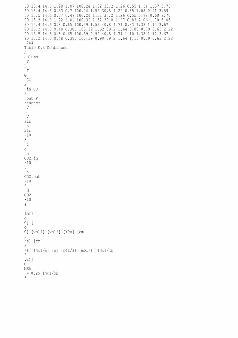
8/10/2019 Erasmus Mass 2004.PDF
http://slidepdf.com/reader/full/erasmus-mass-2004pdf 252/257
60 15.4 14.6 1.28 1.07 100.24 1.52 30.2 1.26 0.55 1.64 1.37 5.7560 15.4 14.6 0.83 0.7 100.24 1.52 30.8 1.29 0.55 1.08 0.91 3.5960 15.5 14.6 0.57 0.47 100.24 1.52 30.2 1.26 0.55 0.72 0.60 2.7090 15.3 14.6 1.22 1.01 100.39 1.52 39.8 1.67 0.83 2.06 1.70 5.0590 15.4 14.6 0.8 0.65 100.39 1.52 40.8 1.71 0.83 1.38 1.12 3.6790 15.2 14.6 0.48 0.385 100.39 1.52 39.2 1.64 0.83 0.79 0.63 2.2290 15.5 14.6 0.8 0.65 100.39 0.99 40.8 1.71 1.10 1.38 1.12 3.6790 15.2 14.6 0.48 0.385 100.39 0.99 39.2 1.64 1.10 0.79 0.63 2.22244Table E.3 Continuedhcolumn TL TG CO2 in CO2 out Preactor VL
Vair nair·103 tc nCO2,in·105 n
CO2,out·105 NCO2·104 [mm] [oC] [oC] [vol%] [vol%] [kPa] [cm
3/s] [cm3/s] [mol/s] [s] [mol/s] [mol/s] [mol/(m2.s)]CMEA = 0.25 [mol/dm3

8/10/2019 Erasmus Mass 2004.PDF
http://slidepdf.com/reader/full/erasmus-mass-2004pdf 253/257
]90 29.9 30.3 0.63 0.55 100.79 1.52 22.4 0.89 0.74 0.57 0.49 1.0290 30.3 30.6 1.2 1.01 100.41 1.52 43.5 1.72 0.74 2.09 1.76 4.7290 30.3 30.5 0.89 0.75 100.41 1.52 43.5 1.73 0.74 1.55 1.30 3.4660 29.9 30.2 1.17 1.03 100.41 1.52 43.3 1.72 0.49 2.04 1.79 5.2060 29.9 30.1 0.88 0.78 100.41 1.52 43.3 1.72 0.49 1.53 1.35 3.70CMEA = 0.3 [mol/dm3]90 15.1 14.2 1.32 1.07 100.54 1.52 43.5 1.83 0.83 2.44 1.97 6.5990 15.7 14.9 1.21 0.97 100.54 1.52 43.7 1.83 0.83 2.24 1.79 6.3290 15.2 14.5 0.92 0.75 100.54 1.52 43.5 1.82 0.83 1.69 1.38 4.4490 15.1 14.5 0.63 0.505 100.54 1.52 43.5 1.82 0.83 1.16 0.93 3.2590 15.4 14.4 1.265 1.04 100.54 0.99 43.7 1.83 1.10 2.35 1.93 5.9590 15.3 14.3 0.9 0.73 100.54 0.99 43.7 1.83 1.11 1.66 1.35 4.4690 15.2 14.3 0.61 0.49 100.54 0.99 43.7 1.83 1.11 1.13 0.90 3.1360 15.2 14.3 1.255 1.09 100.54 1.52 43.7 1.83 0.55 2.33 2.02 6.5560 15.1 14.5 0.92 0.79 100.54 1.52 43.7 1.83 0.55 1.70 1.46 5.1260 15 14.4 0.59 0.5 100.54 1.52 43.7 1.83 0.55 1.09 0.92 3.5260 29.9 30.2 1.32 1.14 100.41 1.52 43.5 1.73 0.49 2.31 1.99 6.7460 29.9 30.2 1.14 0.98 100.41 1.52 43.5 1.73 0.49 1.99 1.71 5.9760 29.9 30.2 0.87 0.75 100.41 1.52 43.5 1.73 0.49 1.52 1.31 4.45
90 30.1 30.2 1.2 0.985 100.41 1.52 43.5 1.73 0.74 2.10 1.72 5.3590 30.1 30.2 0.89 0.72 100.41 1.52 43.5 1.73 0.74 1.55 1.25 4.2090 30.2 30.2 0.61 0.485 100.41 1.52 43.5 1.73 0.74 1.06 0.84 3.08245Table E.4 Experimental results for determination of effective surface area of Flexipac 350YTair(in) Tair(out) Tliq(in) T
liq(out) Pcolumn CO2 in CO2 out CMEA uG,s FG
nair uL,s NCO2·104 Area·104 ae

8/10/2019 Erasmus Mass 2004.PDF
http://slidepdf.com/reader/full/erasmus-mass-2004pdf 254/257
[oC] [oC] [oC] [oC] [kPa] [vol%] [vol%] [mol/dm3] [m3/(m2s)] [(Pa)0.5] [mol/s] [m3/(m2hr)] [mol/(m2s)] [m
2] [m2/m3]FG » 1.1 [(m/s).(kg/m3)0.5]
24.2 24.5 23.4 26.8 99.79 1.05 0.96 0.247 1.07 1.15 1.35 6.1 4.52 3.59 11024.2 23.7 23.2 25.9 99.79 1.05 0.9 0.247 1.06 1.15 1.34 13.6 4.50 3.57 18224.3 23.9 23.6 25.6 99.79 1.05 0.88 0.247 1.06 1.15 1.34 17.8 4.50 3.57 20723.5 24.4 23.5 25.3 99.79 1.03 0.84 0.247 1.06 1.14 1.34 24.7 4.42 3.51 235FG » 1.4 [(m/s).(kg/m3)0.5]23.3 22.5 19.3 24.7 100.66 1.08 1.01 0.280 1.32 1.44 1.72 6.1 5.37 4.26 9221.3 23.3 22 22.6 100.59 1.04 0.9 0.270 1.30 1.42 1.67 13.6 4.89 3.88 196
20.2 20.6 20.4 21.8 100.99 1.05 0.9 0.276 1.31 1.44 1.71 17.8 5.13 4.07 20419.6 20.8 20.4 21.4 100.99 1.05 0.88 0.276 1.31 1.43 1.70 24.7 5.14 4.08 230FG » 2.0 [(m/s).(kg/m3)0.5]19.6 22 21.9 20.8 100.99 1.03 0.97 0.276 1.93 2.11 2.47 6.1 5.03 3.99 121

8/10/2019 Erasmus Mass 2004.PDF
http://slidepdf.com/reader/full/erasmus-mass-2004pdf 255/257
19.7 22.2 21.5 21.2 100.99 1.05 0.95 0.276 1.91 2.09 2.45 13.6 5.16 4.10 19419.5 21.5 20.8 21.4 100.99 1.05 0.94 0.276 1.89 2.07 2.43 17.8 5.21 4.14 20920.6 22 22 22.4 100.59 1.04 0.91 0.270 1.86 2.03 2.39 24.7 5.02 3.99 252
246APPENDIX FBinary VLE for chlorobenzene/ethylbenzene test systemThe recommended vapour pressure for chlorobenzene and ethylbenzene accordingto the IChemE (Onken, 1990) are:Chlorobenzene(1): [ ]( ) [ ]= - +1391.262log P, hPa 7.040849 T C 213.024 (F1)Ethylbenzene(2): [ ]( ) [ ]= - +1412.676log P, hPa 7.063282 T C 211.972 (F2)Regression of the NRTL model (Abbott, 1994) on the experimental VLE data forchlorobenzene/ethylbenzene provided by the IChemE (Onken, 1990) yielded thefollowing results:a12 = -10.5556 [K]a21 = 11.3096 [K]alpha = 0.9 (F3)Experimental dataThe experimental data for Flexipac 350Y and Flexipac 350Y HC are given in TableF.1 and Table F.2. The data for Flexipac 500Y and Flexipac 500Y HC are given in
Table F.3 and Table F.4.247Table F.1 Total reflux distillation experimental results for Flexipac 350Y, chlorobenzene/ethylbenzene systemRunnoConc. CLBZ [wt%] Temperatures [oC] Patm Ptop dP
seg dPtotal* Qreb Qcond Qavg Distillate Bottoms Reboiler Sump 1 2 3 [kPa] [kPa] [mmH
2O] [mmH2O] [kW] [kW] [kW]1 80.53 46.41 135.8 135.3 134.9 134.3 134 101.26 101.26 7.5 34 24.9 19.3 22.12 79.69 44.16 136 135.5 135 134.4 134.2 101.13 101.13 12 60 34.0 28.1 31.13 78.91 42.09 136.2 135.7 135.3 134.6 134.2 101.13 101.13 18 87 40.0 34.4 37.24 78.54 40.51 136.5 135.8 135.4 134.6 134.2 101.13 101.13 23.5 110 44.1 38.1 41.15 78.09 39.7 136.6 135.8 135.5 134.6 134.2 101.19 101.19 28 130 45.3 39.8 42.5

8/10/2019 Erasmus Mass 2004.PDF
http://slidepdf.com/reader/full/erasmus-mass-2004pdf 256/257
6 78.17 37.32 136.8 136 135.6 134.6 134.2 100.99 100.99 50 O/R 50.6 44.9 47.87 78.45 42.01 135.9 135.4 135 134.5 134 100.66 100.66 13 65 34.1 29.7 31.98 77.96 38.85 136.6 135.8 135.4 134.8 134.2 100.59 100.59 32 O/R 46.3 42.2 44.29 82.48 45.36 116.9 116.3 115.7 115.2 114.5 100.86 60.22 9.5 46 25.1 21.4 23.310 81.21 41.37 118 117.4 116.6 115.6 115 100.79 61.00 20 103 35.8 32.5 34.111 80.96 39.79 117 116.3 115.4 114.7 113.8 100.06 58.58 28 138 37.9 34.7 36.312 80.61 48.74 116.9 116.4 115.2 114.5 113.8 100.19 57.86 40 O/R 40.1 35.6 37.913 80.27 37.17 117 116.2 115.4 114.5 113.8 100.19 57.86 48 O/R 41.1 36.0 38.614 80.76 36.68 117.2 117 115.7 114.8 114.2 100.13 57.80 62 O/R 42.6 38.2 40.415 84.85 44.67 94.8 94.4 93.1 92.6 91.9 99.66 29.39 10 50 19.9 16.2 18.116 83.94 41.38 96 95.7 94.3 93 92.6 99.53 30.10 20 110 27.9 25.3 26.617 84.09 39.95 96.3 95.7 94.2 93.3 92.6 99.53 29.26 29 145 30.3 26.2 28.318 83.5 38.2 97 96.6 94.8 94 93.1 99.59 29.32 41 O/R 31.5 28.1 29.819 83.03 36.8 97.2 96.6 95 94 93.1 99.66 29.39 52 O/R 32.7 28.8 30.820 83.21 35.76 98.2 97.6 96 94.8 93.6 99.86 29.59 61 O/R 34.8 31.7 33.3* O/R: value outside measuring range248Table F.2 Total reflux distillation experimental results for Flexipac 350Y HC, chlorobenzene/ethylbenzene systemRunnoConc. CLBZ [wt%] Temperatures [oC] P
atm Ptop dPseg dPtotal* Qreb Qcond Qavg
Distillate Bottoms Reboiler Sump 1 2 3 [kPa] [kPa] [mmH2O] [mmH2O] [kW] [kW] [kW]1 77.89 48.39 135.5 135.1 135 134.5 134.3 100.99 100.99 6 26 22.2 16.7 19.42 78.12 39.55 136.5 136 135.8 134.5 134.4 100.93 100.93 33 147.5 49.3 43.9 46.63 78.74 45.20 135.8 135.4 135 134.6 134.2 100.99 100.99 9 45 27.8 24.0 25.94 77.99 42.37 136 135.6 135.3 134.9 134.2 100.79 100.79 16.5 82 37.8 33.3 35.65 77.42 40.53 136.2 135.9 135.4 134.9 134.4 100.73 100.73 21.5 106.5 43.2 37.4 40.36 76.74 38.16 136.4 136 135.7 135 134.3 100.79 100.79 28 141 46.8 42.3 44.6
7 79.31 39.13 136.7 136.3 135.8 134.9 134.2 100.53 100.53 48 O/R 51.8 49.3 50.58 80.75 48.32 116.4 115.8 115.2 114.8 114.2 100.73 59.24 5.5 26.5 18.6 15.2 16.9 9 82.38 46.21 116.5 116 115.4 114.6 114.2 100.66 59.18 10.5 52.5 25.6 22.7 24.210 81.96 43.79 116.7 116.2 115.5 115 114.2 100.66 59.18 16 85 32.4 28.5 30.511 81.79 42.46 117 116.3 115.5 114.9 114.3 100.79 59.31 21 105.5 35.9 32.2 34.112 81.22 40.65 117.8 117.2 116.2 115.6 114.7 100.93 59.44 29 145 39.6 36.8 38.213 80.33 39.01 118.1 117.5 116.6 115.8 115.1 100.66 60.02 36 O/R 43.3 40.0 41.714 80.11 37.41 117.8 117.3 116.4 115.6 114.7 100.66 59.18 43.5 O/R 45.1 41.3 43.2

8/10/2019 Erasmus Mass 2004.PDF
http://slidepdf.com/reader/full/erasmus-mass-2004pdf 257/257
15 79.64 35.60 118.2 118 116.6 115.7 115 100.66 59.18 62 O/R 47.1 43.2 45.116 85.07 46.42 95 94.6 93.7 93.2 92.2 100.26 29.99 10.5 56.5 20.6 17.7 19.117 85.39 43.08 96.3 95.8 94.6 94 93.1 100.06 29.79 21.5 117 27.8 25.2 26.518 84.60 41.28 97 96.3 95 94.2 93.1 100.06 29.79 30 153 31.8 30.0 30.919 83.65 39.53 97.8 97.3 95.7 94.8 93.6 100.13 29.86 40 O/R 35.4 32.1 33.820 83.97 38.57 97.9 97.3 95.8 94.6 93.4 99.86 29.59 50 O/R 37.7 33.8 35.721 83.71 36.71 98.8 98.2 96.4 95.4 94.2 99.73 29.46 60 O/R 38.5 35.7 37.1* O/R: value outside measuring range