Equivariant Perturbation in

Gomory and Johnson’s Infinite Group Problem.

I. The One-Dimensional Case

Amitabh Basu∗ Robert Hildebrand† Matthias Koppe‡

March 25, 2014

Abstract

We give an algorithm for testing the extremality of minimal valid functions for Gomoryand Johnson’s infinite group problem that are piecewise linear (possibly discontinuous)with rational breakpoints. This is the first set of necessary and sufficient conditions thatcan be tested algorithmically for deciding extremality in this important class of minimalvalid functions. We also present an extreme function that is a piecewise linear functionwith some irrational breakpoints, whose extremality follows from a new principle.

1 Introduction

Cutting planes for mixed integer optimization. Cutting planes are a key ingredientin branch and cut algorithms, the state-of-the-art technology for solving mixed integer op-timization problems. Strong cutting planes for combinatorial optimization problems arisefrom detailed studies of the convex geometry and polyhedral combinatorics of the problem,more specifically of the convex hull of the incidence vectors of feasible solutions. Thousandsof research papers giving sophisticated problem-specific cutting planes (for instance, mostfamously, for the Traveling Salesperson Problem) have appeared since the early 1980s.

In contrast, the state-of-the-art solvers (both commercial and academic) for general mixedinteger optimization problems are based on extremely simple principles of generating cuttingplanes that go back to the 1960s, but whose numerical effectiveness has only been discoveredin the mid-1990s [5].

The optimal simplex tableau, describing an optimal solution to the continuous relaxationof an integer optimization problem

max{ c · x | Ax = b, x ∈ Zn+ } (1)

takes the formxB = A−1B b + (−A−1B AN )xN , xB ∈ ZB+, xN ∈ ZN+ , (2)

∗Dept. of Applied Mathematics and Statistics, The Johns Hopkins University, basu.amitabh@jhu.edu†Dept. of Mathematics, University of California, Davis, rhildebrand@math.ucdavis.edu‡Dept. of Mathematics, University of California, Davis, mkoeppe@math.ucdavis.edu

1

where the subscripts B and N denote the basic and non-basic parts of the solution x andmatrix A, respectively. The widely used, numerically effective general-purpose cuts such asGomory’s mixed integer (GMI) cut [21] are derived by simple integer rounding principlesfrom a single row, corresponding to some basic variable xi, of the tableau:

xi = −fi +∑j∈N

rjxj , xi ∈ Z+, xN ∈ ZN+ .

For example, if a tableau row reads

x1 = −(−45)− 1

5x2 + 25x3 + 11

5 x4,

we can use the GMI formula, which describes a periodic, piecewise linear function πfi : R→ R,to determine the coefficients of a cutting plane, one-by-one:

πfi(−15) = 1

4 , πfi(25) = 3

4 , πfi(115 ) = 1.

Thus, we obtain the (very strong) cutting plane

14x2 + 3

4x3 + x4 ≥ 1. (3)

Unfortunately, the performance of cutting-plane algorithms has stagnated since the com-putational breakthroughs of the late 1990s and early 2000s.

The quest of the effective multi-row cut. To meet the challenges of ever more demand-ing applications, it is necessary to make effective use of information from several rows of thetableau for generating cuts. Finding such effective multi-row cuts is one of the most importantopen questions in cutting plane theory and in practical mixed-integer linear optimization.

The past seven years have seen a revival of so-called intersection cuts, originally introducedby Balas [4] in 1971. This research trend was started by Andersen et al. [1], who consideredthe relaxation

xB = A−1B b + (−A−1B AN )xN , xB ∈ ZB, xN ∈ RN+ .

In this relaxation,

• the basic variables xB are not restricted to be non-negative, but are still required to beintegers;

• the non-basic variables xN are restricted to be non-negative, but are no longer requiredto be integers.

This setup, in which maximal lattice-free convex bodies play a central role, can be studiedusing the classical tools of convex geometry and the Geometry of Numbers and has provedto be a highly fruitful research direction [2, 6, 7]. Unfortunately, the recent numerical studiesof cutting planes based on these techniques have been disappointing; only marginal improve-ments upon the standard GMI cuts have been obtained [28].

2

Gomory’s relaxations revisited. We study a different relaxation, the infinite group prob-lem, which goes back to “classic” work by Gomory [21] in the 1960s and Gomory–Johnson[22, 23] in the 1970s. It is an elegant infinite dimensional generalization of earlier concepts,Gomory’s finite group relaxation and the closely associated corner polyhedron [21]. Boththe finite and the infinite group problem have played a very important role in the theory ofderiving valid cutting planes for integer programming problems, and thus in the foundationalaspects of integer programming. The problems have attracted renewed attention in the pastdecade, with several recent papers discovering very intriguing structures in these problems,and connecting with some deep and beautiful areas of mathematics [3, 8, 9, 13, 14, 16–20, 24, 26, 27]. There remain many significant open problems which provide fertile groundsfor future research. A more detailed discussion of the importance of the infinite group problemcan be found in the recent survey by Conforti, Cornuejols and Zambelli [15].

Gomory’s group relaxation is defined as

xB = A−1B b + (−A−1B AN )xN , xB ∈ ZB, xN ∈ ZN+ . (4)

This relaxation is stronger than the one by Andersen et al., since the non-basic variablesare required to be non-negative integers.

Instead of the full tableau, one can again study just a single row of the tableau, or a fewrows. In the numerical example above, a single-row group relaxation reads:

x1 = −(−45)− 1

5x2 + 25x3 + 11

5 x4, x1 ∈ Z, x2, x3, x4 ∈ Z+.

This equation can be equivalently written as a group equation in R/Z by reading the equationmodulo 1; the variable x1 disappears in this way:

0 ≡ −15 + 4

5x2 + 25x3 + 1

5x4 (mod 1), x2, x3, x4 ∈ Z+.

The example, arising from a basis of determinant q = 5 and all-integer problem data, hastableau data that are multiples of 1

q = 15 . By renaming

x2 = s(45), x3 = s(25), x4 = s(15)

and introducing extra variables s(05), s(35) for every possible coefficient that is a multiple of 1q ,

we obtain the finite master group relaxation

0 ≡ −15 + 0

5 · s(05) + 1

5 · s(15) + 2

5 · s(25) + 3

5 · s(35) + 4

5 · s(45) (mod 1), s(05), . . . , s(45) ∈ Z+,

which only depends on the value fi = 15 and on q = 5. Now we go one step further and

introduce infinitely many new variables s(r) for every r ∈ R, viz., a function s : R→ Z+, andobtain the infinite group relaxation

0 ≡ −15 +

∑r∈R

r · s(r) (mod 1), s : R→ Z+ a function of finite support,

which only depends on the value fi = 15 .

3

Formal definition of the problem. More formally, Gomory’s group problem [21] con-siders an abelian group G, written additively, and studies the set of functions s : G → Rsatisfying the following constraints: ∑

r∈Grs(r) ∈ f + S (5)

s(r) ∈ Z+ for all r ∈ Gs has finite support,

where f is a given element in G, and S is a subgroup of G (not necessarily of finite indexin G); so f + S is the coset containing the element f .

In particular, we are interested in studying the convex hull Rf (G,S) of all functionssatisfying the constraints in (5). Observe that Rf (G,S) is a convex subset of the (possiblyinfinite-dimensional) vector space V of functions s : G→ R with finite support.

An important case is the infinite group problem, where G = Rk is taken to be the groupof real vectors under addition, and S = Zk is the subgroup of the integral vectors. In thispaper, we are considering the one-dimensional case of the infinite group problem, i.e., k = 1.This is an important stepping stone for the larger goal of effective multi-row cuts. We extendour results to the case k = 2 in [10–12].

Valid inequalities and valid functions. Any linear inequality in V is given by a pair(π, α) where π is a function π : G → R (not necessarily of finite support) and α ∈ R. Thelinear inequality is then given by

∑r∈G π(r)s(r) ≥ α; the left-hand side is a finite sum

because s has finite support. Such an inequality is called a valid inequality for Rf (G,S) if∑r∈G π(r)s(r) ≥ α for all s ∈ Rf (G,S).For historical and technical reasons, we concentrate on those valid inequalities for which

π ≥ 0. This implies that we can choose, after a scaling, α = 1. Thus, we only focus onvalid inequalities of the form

∑r∈G π(r)s(r) ≥ 1 with π ≥ 0. Such functions π will be

termed valid functions for Rf (G,S). As pointed out in [15], the non-negativity assumptionin the definition of a valid function might seem artificial at first. Although there exist validinequalities

∑r∈R π(r)s(r) ≥ α for Rf (R,Z) such that π(r) < 0 for some r ∈ R, it can be

shown that π must be non-negative over all rational r ∈ Q. Since data in integer programsare usually rational, it is natural to focus on non-negative valid functions.

A valid function immediately gives the coefficients of a cutting plane for Gomory’s grouprelaxation (4) and thus the original integer optimization problem (1), as the GMI functiondid in the example of (3).

Minimal and extreme functions. Gomory and Johnson [22, 23] defined a hierarchy onthe set of valid functions, capturing the strength of the corresponding valid inequalities, whichwe summarize now. A valid function π for Rf (G,S) is said to be minimal for Rf (G,S) ifthere is no valid function π′ 6= π such that π′(r) ≤ π(r) for all r ∈ G. It is known that forevery valid function π for Rf (G,S), there exists a minimal valid function π′ such that π′ ≤ π(see [13] for a proof in the case when G = Rk, S = Zk). Also minimal valid functions πsatisfy π(r) ≤ 1 for r ∈ G [15]. Since s ∈ Rf (G,S) are always non-negative functions,

4

minimal functions clearly dominate valid functions that are not minimal, making the latterredundant in the description of Rf (G,S).

A stronger notion is that of an extreme function. A valid function π is extreme forRf (G,S) if it cannot be written as a convex combination of two other valid functions forRf (G,S), i.e., π = 1

2(π1 + π2) implies π = π1 = π2. It is easy to verify that extremefunctions are minimal. Minimal functions for Rf (G,S) were well characterized by Gomoryfor groups G such that S has finite index in G in [21], and later for Rf (R,Z) by Gomory andJohnson [22]. We state these results in a unified notation in the following theorem, whichhas the same proof as the theorem in [22].

A function π : G → R is subadditive if π(x + y) ≤ π(x) + π(y) for all x, y ∈ G. We saythat π is symmetric (or satisfies the symmetry condition) if π(x)+π(f −x) = 1 for all x ∈ G.

Theorem 1.1 (Gomory [21], Gomory and Johnson [22]). Let π : G → R be a non-negativefunction. Then π is a minimal valid function for Rf (G,S) if and only if π(r) = 0 for allr ∈ S, π is subadditive, and π satisfies the symmetry condition. The first two conditionsimply that π is periodic modulo S (i.e., constant over any coset of S).

Remark 1.2. Note that this implies that one can view a minimal valid function π as afunction from G/S to R, and thus studying Rf (G,S) is the same as studying Rf (G/S, 0).However, we avoid this viewpoint in this paper.

All classes of extreme functions described in the literature are piecewise linear, with theexception of a family of measurable functions constructed in [9]. However, a tight charac-terization of extreme functions for Rf (R,Z) has eluded researchers for the past four decadesnow.

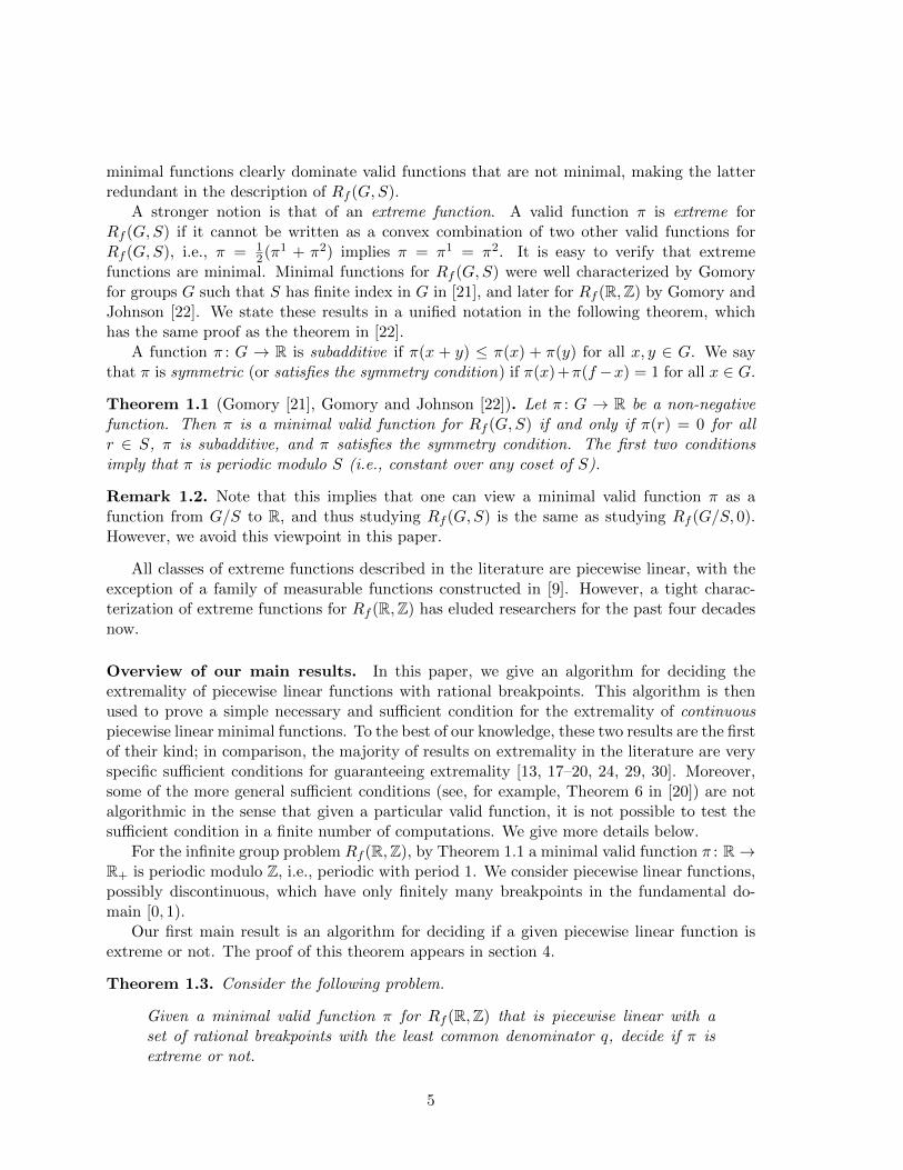
Overview of our main results. In this paper, we give an algorithm for deciding theextremality of piecewise linear functions with rational breakpoints. This algorithm is thenused to prove a simple necessary and sufficient condition for the extremality of continuouspiecewise linear minimal functions. To the best of our knowledge, these two results are the firstof their kind; in comparison, the majority of results on extremality in the literature are veryspecific sufficient conditions for guaranteeing extremality [13, 17–20, 24, 29, 30]. Moreover,some of the more general sufficient conditions (see, for example, Theorem 6 in [20]) are notalgorithmic in the sense that given a particular valid function, it is not possible to test thesufficient condition in a finite number of computations. We give more details below.

For the infinite group problem Rf (R,Z), by Theorem 1.1 a minimal valid function π : R→R+ is periodic modulo Z, i.e., periodic with period 1. We consider piecewise linear functions,possibly discontinuous, which have only finitely many breakpoints in the fundamental do-main [0, 1).

Our first main result is an algorithm for deciding if a given piecewise linear function isextreme or not. The proof of this theorem appears in section 4.

Theorem 1.3. Consider the following problem.

Given a minimal valid function π for Rf (R,Z) that is piecewise linear with aset of rational breakpoints with the least common denominator q, decide if π isextreme or not.

5

There exists an algorithm for this problem that takes a number of elementary operations overthe reals that is bounded by a polynomial in q.

If we start with any piecewise linear valid function π, the first step is to determine if π isminimal. A minimality test for continuous piecewise linear functions was given by Gomoryand Johnson (see Theorem 7 in [24]). In section 2.2 we present a minimality test that worksfor discontinuous functions too.

Next we investigate the precise relationship between continuous extreme functions for theinfinite group problem and certain finite group problems, i.e., Rf (G,Z) where G is a discretesubgroup of R that contains Z. (The word “finite” refers to the finite index of Z in G, inother words the quotient group G/Z is finite.) A first result in this direction appeared in[20]; we state it in our notation.

Theorem 1.4 (Theorem 6 in [20]). Let π be a piecewise linear minimal valid function forRf (R,Z) with set B of rational breakpoints with the least common denominator q. LetG2n , n ∈ N denote the subgroups 1

2nqZ. Then π is extreme if and only if the restrictionπ|G2n

is extreme for Rf (G2n ,Z) for all n ∈ N.

Clearly the above condition cannot be checked in a finite number of steps and hencecannot be converted into an algorithm, because it potentially needs to test infinitely manyfinite group problems. In contrast, we prove the following result in section 4.

Theorem 1.5. Let π be a continuous piecewise linear minimal valid function for Rf (R,Z)

with set B of rational breakpoints with the least common denominator q. Let G = 14qZ. Then

π is extreme for Rf (R,Z) if and only if π|G is extreme for Rf (G,Z).

Gomory gives a characterization of extreme valid functions for finite group problems via alinear program. This provides an alternative algorithm for testing extremality of continuouspiecewise linear functions with rational breakpoints, under the light of Theorem 1.5. Ofcourse, Theorem 1.3 is more general as it provides an algorithm for discontinuous functionsalso.

Techniques of this paper. The standard technique for showing extremality is to supposethat π = 1

2(π1 +π2), where π1, π2 are other valid functions. One observes the following basicfact:

Lemma 1.6. Let π be minimal, π = 12(π1 + π2) with π1, π2 valid functions. Then π1, π2 are

minimal, and all subadditivity relations π(x + y) ≤ π(x) + π(y) that are tight for π are alsotight for π1, π2.

Then one shows that actually π = π1 = π2 holds. The main tool used in the literaturefor showing this is the so-called Interval Lemma introduced by Gomory and Johnson in [24],which we state here for a more coherent discussion of the new ideas in this paper.

Lemma 1.7 (Interval Lemma [9, 24]). Let θ : R→ R be a function bounded on every boundedinterval. Given real numbers u1 < u2 and v1 < v2, let U = [u1, u2], V = [v1, v2], and

6

U + V = [u1 + v1, u2 + v2]. If θ(u) + θ(v) = θ(u+ v) for every u ∈ U and v ∈ V , then thereexists c ∈ R such that

θ(u) = θ(u1) + c(u− u1) for every u ∈ U ,

θ(v) = θ(v1) + c(v − v1) for every v ∈ V ,

θ(w) = θ(u1 + v1) + c(w − u1 − v1) for every w ∈ U + V .

Remark 1.8. We remark that the Interval Lemma is a lemma of real analysis (the theoryof functional equations); the hypothesis that the function θ is bounded on every boundedinterval is one of several possible hypotheses to rule out certain pathological functions.

Every proof of extremality in the existing literature employs the Interval Lemma on properintervals that satisfy certain additivity conditions to deduce affine linearity properties thatπ1 and π2 share with π. This is followed by a linear algebra argument (explicit in Gomory–Johnson’s proof of the two slope theorem, but implicit in many other proofs) to establishuniqueness of π, and thus its extremality.

Surprisingly, the arithmetic (number-theoretic) aspects of the problem seem to have beenlargely overlooked, even though they are at the core of the theory of the closely relatedfinite group problem. This aspect turns out to be the key for completing the algorithmicclassification of extreme piecewise linear functions.

To capture the relevant arithmetics of the problem, we study finite sets of additivityrelations of the form π(ti) + π(y) = π(ti + y) and π(x) + π(ri − x) = π(ri), where the pointsti and ri are certain breakpoints of the function π. They give rise to a useful abstraction, thereflection group Γ generated by the reflections ρri : x 7→ ri−x and translations τti : y 7→ ti+y.

We then study the natural action of the reflection group Γ on the set of open intervalsdelimited by the elements of G = 1

qZ. Roughly speaking, the action of Γ transfers the affinelinearity established by the Interval Lemma on some interval I to the orbit Γ(I). Actually,this transfer is more delicate, and we have to combine this arithmetic consideration with adiscussion of reachability. In the end, the transfer happens within each connected componentof a certain graph.

When the Interval Lemma and this transfer technique establish affine linearity of π1, π2

on all intervals where π is affinely linear, we can proceed with linear algebra techniques todecide extremality of π. Otherwise, we show that there is a way to perturb π slightly toconstruct distinct minimal valid functions π1 = π + π and π2 = π − π. Here the reflectiongroup Γ gives a blueprint for this perturbation in the following way. We use Γ-equivariantfunctions, i.e., functions that are invariant under translation by 1

q and odd with respect to the

reflection points 0,± 12q ,±

1q , . . . . Sufficiently small Γ-equivariant functions, again modified by

restriction to a certain connected component, are then suitable perturbation functions π. Aparticular choice of these functions allows us to prove Theorem 1.5.

An interesting irrational function and a complexity conjecture. We now discussthe complexity of the algorithm of Theorem 1.3. For the purpose of this discussion, let usrestrict ourselves to a version of the problem where all input data are rational. It is anopen question whether the pseudo-polynomial complexity of our algorithm is best possible,or whether there exists a polynomial-time algorithm, or even a strongly polynomial-time

7

algorithm, whose running time would only depend on the number of breakpoints but not onthe sizes of the denominators. We conjecture that the problem (in a suitable version with allrational input data) is NP-hard in the weak sense.

We believe that the problem is intrinsically arithmetic, so that an algorithm that isoblivious to the sizes of the denominators is not possible. To substantiate this, we constructa certain extreme function with irrational breakpoints (section 5). Any nearby function withrational breakpoints that uses the same construction turns out to not be extreme.

The proof of extremality of this function requires another technique unrelated to theInterval Lemma. Here a reflection group Γ arises under which every point x has an orbit Γ(x)that is dense in R. Roughly speaking (ignoring the reachability issues, which our proof has todiscuss), there exists no non-trivial continuous Γ-equivariant perturbation. Thus the functionis extreme.

2 Preliminaries

2.1 Polyhedral complexes and piecewise linear functions

We introduce the notion of polyhedral complexes, which serves two purposes in our paper.One, it provides an elegant framework to define discontinuous piecewise linear functions.Two, it is a tool for studying subadditivity relations.

Definition 2.1. A (locally finite) polyhedral complex is a collection P of polyhedra in Rksuch that:

(i) if P ∈ P, then all faces of P (including the empty face ∅) are in P,

(ii) the intersection P ∩Q of two polyhedra P,Q ∈ P is a face of both P and Q,

(iii) any compact subset of Rk intersects only finitely many faces in P.

The polyhedral complex P is called periodic modulo Zk if for all P ∈ P and all vectors t ∈ Zk,the translated polyhedron P + t also is in P.

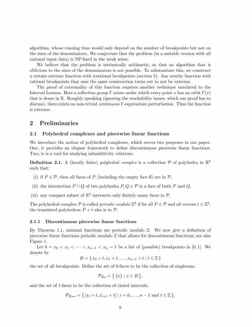
2.1.1 Discontinuous piecewise linear functions

By Theorem 1.1, minimal functions are periodic modulo Z. We now give a definition ofpiecewise linear functions periodic modulo Z that allows for discontinuous functions; see alsoFigure 1.

Let 0 = x0 < x1 < · · · < xn−1 < xn = 1 be a list of (possible) breakpoints in [0, 1]. Wedenote by

B = {x0 + t, x1 + t, . . . , xn−1 + t | t ∈ Z }

the set of all breakpoints. Define the set of 0-faces to be the collection of singletons,

PB, ={{x} | x ∈ B

},

and the set of 1-faces to be the collection of closed intervals,

PB, ={

[xi + t, xi+1 + t] | i = 0, . . . , n− 1 and t ∈ Z}.

8

J

xi+1 xi+2

πK

I K

xi

πI

πJ

Figure 1: A discontinuous piecewise linear function π with breakpoints B = {x0, . . . , xn}+Zwith 0 = x0 < x1 < · · · < xn = 1. This figure shows a piecewise linear function π on(xi, xi+2) where I = [xi, xi+1], J = {xi+1},K = [xi+1, xi+2]. Affine linear functions πI , πJ ,πK are defined on all of R. The piecewise linear function π agrees with πI on rel int(I), etc.

Then PB = {∅} ∪ PB, ∪ PB, is a locally finite one-dimensional polyhedral complex that isperiodic modulo Z.

For each 0-face I ∈ PB, , there is a constant function πI(x) = bI ; for each 1-face I ∈ PB, ,there is an affine linear function πI(x) = mIx + bI , defined for all x ∈ R. A functionπ : R→ R+ periodic modulo Z is called piecewise linear if it is given by π(x) = πI(x) wherex ∈ rel int(I) for some I ∈ PB.

Since π is periodic modulo Z, for any t ∈ Z we have πI+t(x+ t) = πI(x) for I ∈ PB andthus bI+t = bI for I ∈ PB, and mI+t = mI , bI+t = bI −mIt for I ∈ PB, .

2.1.2 A two-dimensional polyhedral complex

The following notation will be used in the rest of the paper. The function ∆π measures theslack in the subadditivity constraints:

∆π(x, y) = π(x) + π(y)− π(x+ y).

Let ∆PB be the two-dimensional polyhedral complex with faces

F = F (I, J,K) = { (x, y) ∈ R2 | x ∈ I, y ∈ J, x+ y ∈ K },

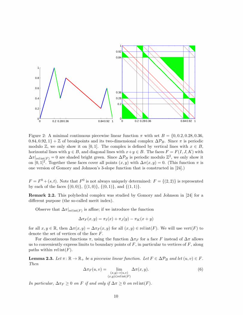
where I, J,K ∈ PB, ∪ PB, ; see Figure 2.Since PB is periodic modulo Z, the complex ∆PB is periodic modulo Z2. By construction,

all faces F of the complex are polytopes (i.e., points, edges, or convex polygons), and thefaces contained in [0, 1]2 form a finite system of representatives, i.e., for every face F ∈ ∆PB,there exists a face F 0 ∈ ∆PB with F 0 ⊆ [0, 1]2 and a translation vector (s, t) ∈ Z2 such that

9

0 0.2 0.28 0.36 0.84 0.92 10

0.2

0.4

0.6

0.8

1

0 0.2 0.28 0.36 0.84 0.92 10

0.2

0.28

0.36

0.84

0.92

1

Figure 2: A minimal continuous piecewise linear function π with set B = {0, 0.2, 0.28, 0.36,0.84, 0.92, 1} + Z of breakpoints and its two-dimensional complex ∆PB. Since π is periodicmodulo Z, we only show it on [0, 1]. The complex is defined by vertical lines with x ∈ B,horizontal lines with y ∈ B, and diagonal lines with x+y ∈ B. The faces F = F (I, J,K) with∆π|rel int(F ) = 0 are shaded bright green. Since ∆PB is periodic modulo Z2, we only show iton [0, 1]2. Together these faces cover all points (x, y) with ∆π(x, y) = 0. (This function π isone version of Gomory and Johnson’s 3-slope function that is constructed in [24].)

F = F 0 + (s, t). Note that F 0 is not always uniquely determined: F = {(2, 2)} is representedby each of the faces {(0, 0)}, {(1, 0)}, {(0, 1)}, and {(1, 1)}.

Remark 2.2. This polyhedral complex was studied by Gomory and Johnson in [24] for adifferent purpose (the so-called merit index).

Observe that ∆π|rel int(F ) is affine; if we introduce the function

∆πF (x, y) = πI(x) + πJ(y)− πK(x+ y)

for all x, y ∈ R, then ∆π(x, y) = ∆πF (x, y) for all (x, y) ∈ rel int(F ). We will use vert(F ) todenote the set of vertices of the face F .

For discontinuous functions π, using the function ∆πF for a face F instead of ∆π allowsus to conveniently express limits to boundary points of F , in particular to vertices of F , alongpaths within rel int(F ).

Lemma 2.3. Let π : R→ R+ be a piecewise linear function. Let F ∈ ∆PB and let (u, v) ∈ F .Then

∆πF (u, v) = lim(x,y)→(u,v)

(x,y)∈rel int(F )

∆π(x, y). (6)

In particular, ∆πF ≥ 0 on F if and only if ∆π ≥ 0 on rel int(F ).

10

Proof. This follows from the definition of ∆πF and the continuity of the affine functions πI ,πJ , and πK .

2.2 Finite test for minimality of piecewise linear functions

By Theorem 1.1, we can test whether a function is minimal by testing subadditivity and thesymmetry condition.

A finite subadditivity test for continuous piecewise linear functions was given by Gomoryand Johnson [24, Theorem 7].1 It easily extends to the discontinuous case. We include aproof in our notation to make the present paper self-contained, but do not claim novelty.Richard, Li, and Miller [30, Theorem 22], for example, presented a superadditivity test fordiscontinuous piecewise linear functions.

We first show that f must be a breakpoint of any minimal valid function.

Lemma 2.4. If π : R→ R is a minimal valid function with breakpoints in B, then f ∈ B.

Proof. Since π is minimal, we have 0 ≤ π ≤ 1. Now, suppose that f /∈ B, i.e., f ∈ int(I) forsome I ∈ PB, . Symmetry and the condition that π(0) = 0 imply that π(f) = 1. Since π ≤ 1and π is affine in int(I), it follows that π ≡ 1 on int(I). The interval f − I contains the originin its interior and by symmetry, π ≡ 0 on int(f − I). Let J be the largest interval containingthe origin such that π ≡ 0 on J and let x = sup{x ∈ J }. Since J is the largest such interval,and x 6= ∞, for every small ε > 0, there exists a point y ≥ x such that ε, y − ε ∈ J andπ(y) > 0. But then π(ε) + π(y− ε) = 0 < π(y), which violates subadditivity, and therefore isa contradiction.

Theorem 2.5 (Minimality test). A piecewise linear function π : R → R with breakpoints Bthat is periodic modulo Z is minimal if and only if the following conditions hold:

1. π(0) = 0.

2. Subadditivity test: For all F ∈ ∆PB with F ⊆ [0, 1]2, we have that ∆πF (u, v) ≥ 0 forall (u, v) ∈ vert(F ).

3. Symmetry test: π(f) = 1, and for all F ∈ ∆PB with

F ⊆{

(x, y) ∈ [0, 1]2∣∣ x+ y ≡ f (mod 1)

},

we have that ∆πF (u, v) = 0 for all (u, v) ∈ vert(F ).

Proof. We use the characterization of minimal functions given by Theorem 1.1.Let F ∈ ∆PB with F ⊆ [0, 1]2 and let (u, v) ∈ vert(F ). Then, by Lemma 2.3,

∆πF (u, v) = lim(x,y)→(u,v)

(x,y)∈rel int(F )

∆π(x, y). (7)

Since π is subadditive by Theorem 1.1, ∆π(x, y) ≥ 0 for all x, y ∈ [0, 1], and therefore thelimit above is also non-negative. Suppose F ⊆ { (x, y) ∈ [0, 1]2 | x + y ≡ f (mod 1) }.

1Note that the word “minimal” needs to be replaced by “satisfies the symmetry condition” throughout thestatement of their theorem and its proof.

11

Since π is symmetric by Theorem 1.1, we have π(x) + π(f − x) = 1 = π(f) and therefore∆π(x, f − x) = 0 for x ∈ [0, 1]. Since π is also periodic modulo Z by Theorem 1.1, we have∆π(x, y) = 0 whenever x + y ≡ f (mod 1) and x, y ∈ [0, 1]. Therefore, the above limit is infact a limit of zeros, and ∆πF (u, v) = 0.

We now show that the stated conditions are sufficient.For subadditivity, we need to show that ∆π(x, y) ≥ 0 for all x, y ∈ R. Since π is periodic

modulo 1, it suffices to show that ∆π(x, y) ≥ 0 for x, y ∈ [0, 1]. Let x, y ∈ [0, 1], then(x, y) ∈ rel int(F ) for some unique F ∈ ∆PB with F ⊆ [0, 1]2 and ∆π(x, y) = ∆πF (x, y).Since ∆πF (u, v) ≥ 0 for all (u, v) ∈ vert(F ), by convexity (∆πF is affine), ∆πF (x, y) ≥ 0.Therefore π is subadditive.

Similarly, to show symmetry, because π is periodic modulo 1, it suffices to show that∆π(x, y) = 0 for all x, y ∈ [0, 1] such that x + y ≡ f (mod 1). Let x, y ∈ [0, 1] such thatx + y ≡ f (mod 1). Since f ∈ B by Lemma 2.4, (x, y) ∈ rel int(F ) for some F ∈ ∆PB forF ⊆ { (x, y) ∈ [0, 1]2 | x+ y ≡ f (mod 1) }. Since ∆πF (u, v) = 0 for all (u, v) ∈ vert(F ), and∆πF is affine, it follows that ∆π(x, y) = ∆πF (x, y) = 0.

Remark 2.6. This theorem implies that, for n = |B ∩ [0, 1)|, there are O(n2) pairs thatneed to be checked in order to check subadditivity, and only O(n) points that need to beevaluated to check for symmetry. These follow from the fact that there are O(n) hyperplanes(lines) in the two-dimensional polyhedral complex ∆PB in [0, 1]2. Any 0-dimensional face(vertex) is at the intersection of at least two hyperplanes (lines), therefore, at most

(O(n)2

)possibilities. And any 0-dimensional face (vertex) corresponding to a symmetry condition isat the intersection of the hyperplane (line) x + y = f or x + y = f + 1 and any other one,therefore, at most O(n) such points.

2.3 Limit relations

Let π be a minimal valid function that is piecewise linear. Suppose π1 and π2 are minimalvalid functions such that π = 1

2(π1+π2). By Lemma 1.6, whenever π(x)+π(y) = π(x+y), thefunctions π1 and π2 must also satisfy this equality relation, that is, πi(x) +πi(y) = πi(x+y).Let ∆πi(x, y) = πi(x) + πi(y)− πi(x+ y) for i = 1, 2. Equivalently, whenever ∆π(x, y) = 0,we also have ∆πi(x, y) = 0 for i = 1, 2. This is easy to see since π, π1, π2 are subadditive,∆π,∆π1,∆π2 ≥ 0 and ∆π = 1

2(∆π1 + ∆π2). We extend this idea slightly, which allows usto handle the discontinuous case conveniently.

Lemma 2.7. Let π : R → R+ be a piecewise linear minimal valid function. Suppose π =12(π1 + π2), where π1 and π2 are valid functions. Let F ∈ ∆PB and let (u, v) ∈ F . If∆πF (u, v) = 0 then

lim(x,y)→(u,v)

(x,y)∈rel int(F )

∆πi(x, y) = 0 for i = 1, 2.

Proof. From definition of ∆π1,∆π2, we see that ∆π = 12(∆π1+∆π2). By Lemma 1.6, π1, π2

are minimal and thus ∆πi ≥ 0 for i = 1, 2. If ∆πF (u, v) = 0, then, using Lemma 2.3,

0 = ∆πF (u, v) = lim(x,y)→(u,v)

(x,y)∈rel int(F )

∆π(x, y) = lim(x,y)→(u,v)

(x,y)∈rel int(F )

12

(∆π1(x, y) + ∆π2(x, y)

).

12

Since the right hand side limit is zero and ∆π1,∆π2 ≥ 0, we must have that

0 = lim(x,y)→(u,v)

(x,y)∈rel int(F )

∆π1(x, y) = lim(x,y)→(u,v)

(x,y)∈rel int(F )

∆π2(x, y).

2.4 Continuity results

We will need the following lemma and theorem on continuity. Although similar results appearin [23], we provide proofs of these facts to keep this paper more self-contained.

Lemma 2.8. If θ : R → R is a subadditive function and lim suph→0|θ(h)h | = L < ∞, then

θ(h) is Lipschitz continuous with Lipschitz constant L.

Proof. Fix any δ > 0. Since lim suph→0|θ(h)h | = L, there exists ε > 0 such that for any

x, y ∈ R satisfying |x − y| < ε, |θ(x−y)||x−y| < L + δ. By subadditivity, |θ(x − y)| ≥ |θ(x) − θ(y)|and so |θ(x)−θ(y)||x−y| < L + δ for all x, y ∈ R satisfying |x − y| < ε. This immediately implies

that for all x, y ∈ R, |θ(x)−θ(y)||x−y| < L + δ, by simply breaking the interval [x, y] into equalsubintervals of size at most ε. Since the choice of δ was arbitrary, this shows that for everyδ > 0, |θ(x)−θ(y)||x−y| < L + δ and therefore, |θ(x)−θ(y)||x−y| ≤ L. Therefore, θ is Lipschitz continuouswith Lipschitz constant L.

Theorem 2.9. Let π : R→ R be a minimal valid function and π = 12(π1 + π2), where π1, π2

are valid functions. Suppose lim suph→0|π(h)h | < ∞. Then this condition also holds for π1

and π2. This implies that π, π1 and π2 are all Lipschitz continuous.

Proof. By Lemma 1.6, π1, π2 are minimal and thus subadditive. Since we assume π1, π2 ≥ 0,π = 1

2(π1+π2) implies that πi ≤ 2π for i = 1, 2. Therefore if lim suph→0|π(h)h | = L <∞, then

lim suph→0|πi(h)h | ≤ 2L < ∞ for i = 1, 2. Applying Lemma 2.8, we get Lipschitz continuity

for all three functions.

2.5 Finitely generated reflection groups from additivity relations

We need to study the pairs (u, v) where the subadditivity condition is satisfied at equality,i.e., π(u) + π(v) = π(u+ v), or, equivalently, ∆π(u, v) = 0. By Lemma 1.6, these additivityrelations also hold for subadditive functions π1, π2 if π = 1

2(π1 + π2). By introducing thedifference function (perturbation) π = π1−π, we can write π1 = π+ π and π2 = π− π. Thenit follows that the same additivity relations also hold for π.

The standard way to use these additivity relations is via the Interval Lemma (Lemma 1.7),where one looks for closed non-degenerate intervals U , V , and W = U + V such that

π(u) + π(v) = π(u+ v) for all u ∈ U and v ∈ V with u+ v ∈W .

We will follow this standard way in section 4.1, where we also extend it by a “patching”technique to cases where W is a subset of the Minkowski sum U + V .

13

In this section, we develop a new way to use these additivity relations, which complementsthe use of the Interval Lemma. Here we consider such relations when one of U , V , or W isa single point, instead of a non-degenerate interval, and W is not necessarily the Minkowskisum of U and V . Let us assume that π : R→ R satisfies finitely many classes of relations ofthe type

π(ti) + π(y) = π(ti + y), i = 1, . . . ,m (8a)

for all y in some interval Yi and

π(x) + π(ri − x) = π(ri), i = 1, . . . , n (8b)

for all x in some interval Xi, where t1, . . . , tm and r1, . . . , rn are finitely many points in R.Under some conditions we will be able to construct a perturbation π that also satisfies all

equations (8). Our strategy is to first construct a function ψ that satisfies more conditions,namely equation (8a) for all y ∈ R and equation (8b) for all x ∈ R.

For this construction we use methods of group theory [25], which provide fundamentalinsights into the structure of the perturbations. Readers who are unfamiliar with the termi-nology of group theory may skip the following development and verify Lemma 2.16 below byelementary means. This will be sufficient for following the proofs of the main theorems ofthis paper, which are proved in section 4. However, the construction of the extreme functionwith irrational breakpoints in section 5 requires the group theoretic tools of this section.

We consider a subgroup of the group Aff(R) of invertible affine linear transformationsof R as follows.

Definition 2.10. For a point r ∈ R, define the reflection ρr : R→ R, x 7→ r−x. For a vectort ∈ R, define the translation τt : R→ R, x 7→ x+ t.

Given a finite number of points r1, . . . , rn and a finite number of vectors t1, . . . , tm, wewill define the subgroup

Γ = 〈ρr1 , . . . , ρrn , τt1 , . . . , τtm〉

that is generated by the listed translations and reflections. Figure 3 shows examples of suchfinitely generated reflection groups.

Let r, s, w, t ∈ R. Each reflection is an involution: ρr ◦ ρr = id, two reflections give onetranslation: ρr ◦ ρs = τr−s. Thus, if we assign a character χ(ρr) = −1 to every reflection andχ(τt) = +1 to every translation, then this extends to a group character of Γ, that is, a grouphomomorphism χ : Γ→ {±1} ⊂ C×.

On the other hand, not all pairs of reflections need to be considered: ρs ◦ ρw = (ρs ◦ ρr) ◦(ρr ◦ ρw) = (ρr ◦ ρs)−1 ◦ (ρr ◦ ρw). Thus the subgroup Γ+ = ker(χ) = { γ ∈ Γ | χ(γ) = +1 }of translations in Γ is generated as follows.

Γ+ = 〈τr2−r1 , . . . , τrn−r1 , τt1 , . . . , τtm〉.

It is normal in Γ, as it is stable by conjugation by any reflection: ρr ◦ τt ◦ ρ−1r = τ−t.In the following, we assume that n ≥ 1, i.e., at least one of the generators is a reflection.

Now, if γ ∈ Γ is not a translation, i.e., χ(γ) = −1, then it is generated by an odd numberof reflections, and thus can be written as γ = τ ◦ ρr1 with τ ∈ Γ+. Thus Γ/Γ+ ∼= 〈ρr1〉 is oforder 2. In short, we have the following lemma.

14

(a)

ρ3/4

134

380

(b)

τ3/8

0 134

38

(c)

ρ3/4

0 134

38

12

τ1/4

ρ3/4ρ1

14

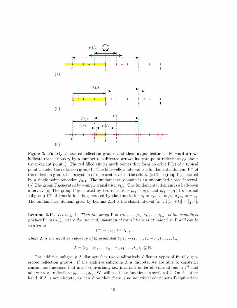
Figure 3: Finitely generated reflection groups and their major features. Forward arrowsindicate translations τt by a number t, bidirected arrows indicate point reflections ρr aboutthe invariant point r

2 . The red filled circles mark points that form an orbit Γ(x) of a typicalpoint x under the reflection group Γ. The blue-yellow interval is a fundamental domain V + ofthe reflection group, i.e., a system of representatives of the orbits. (a) The group Γ generatedby a single point reflection ρ3/4. The fundamental domain is an unbounded closed interval.(b) The group Γ generated by a single translation τ3/8. The fundamental domain is a half-openinterval. (c) The group Γ generated by two reflections ρr1 = ρ3/4 and ρr2 = ρ1. Its normalsubgroup Γ+ of translations is generated by the translation τt = τr2−r1 = ρr2 ◦ ρr1 = τ1/4.

The fundamental domain given by Lemma 2.14 is the closed interval [12r1,12(r1 + t)] = [14 ,

38 ].

Lemma 2.11. Let n ≥ 1. Then the group Γ = 〈ρr1 , . . . , ρrn , τt1 , . . . , τtm〉 is the semidirectproduct Γ+o 〈ρr1〉, where the (normal) subgroup of translations is of index 2 in Γ and can bewritten as

Γ+ = { τt | t ∈ Λ },

where Λ is the additive subgroup of R generated by r2 − r1, . . . , rn − r1, t1, . . . , tm,

Λ = 〈r2 − r1, . . . , rn − r1, t1, . . . , tm〉Z ⊆ R.

The additive subgroup Λ distinguishes two qualitatively different types of finitely gen-erated reflection groups. If the additive subgroup Λ is discrete, we are able to constructcontinuous functions that are Γ-equivariant, i.e., invariant under all translations in Γ+ andodd w.r.t. all reflections ρr1 , . . . , ρrn . We will use these functions in section 4.2. On the otherhand, if Λ is not discrete, we can show that there is no nontrivial continuous Γ-equivariant

15

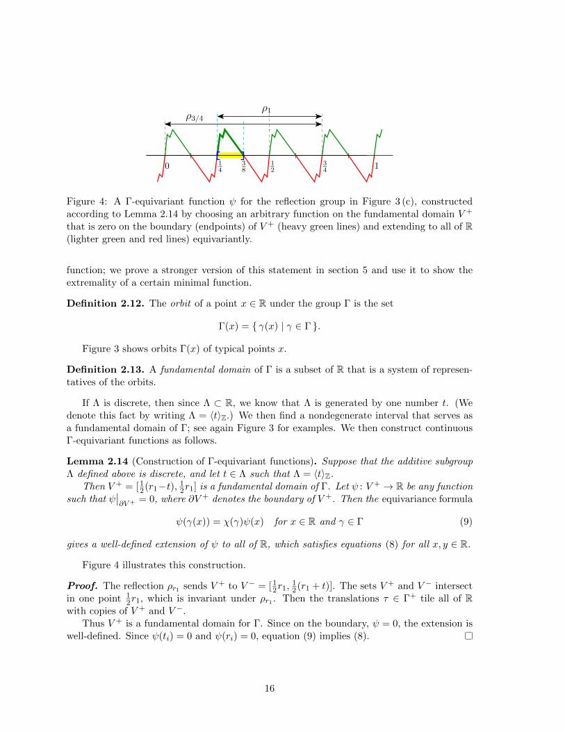
1120 3

438

ρ3/4ρ1

14

Figure 4: A Γ-equivariant function ψ for the reflection group in Figure 3 (c), constructedaccording to Lemma 2.14 by choosing an arbitrary function on the fundamental domain V +

that is zero on the boundary (endpoints) of V + (heavy green lines) and extending to all of R(lighter green and red lines) equivariantly.

function; we prove a stronger version of this statement in section 5 and use it to show theextremality of a certain minimal function.

Definition 2.12. The orbit of a point x ∈ R under the group Γ is the set

Γ(x) = { γ(x) | γ ∈ Γ }.

Figure 3 shows orbits Γ(x) of typical points x.

Definition 2.13. A fundamental domain of Γ is a subset of R that is a system of represen-tatives of the orbits.

If Λ is discrete, then since Λ ⊂ R, we know that Λ is generated by one number t. (Wedenote this fact by writing Λ = 〈t〉Z.) We then find a nondegenerate interval that serves asa fundamental domain of Γ; see again Figure 3 for examples. We then construct continuousΓ-equivariant functions as follows.

Lemma 2.14 (Construction of Γ-equivariant functions). Suppose that the additive subgroupΛ defined above is discrete, and let t ∈ Λ such that Λ = 〈t〉Z.

Then V + = [12(r1−t), 12r1] is a fundamental domain of Γ. Let ψ : V + → R be any functionsuch that ψ

∣∣∂V + = 0, where ∂V + denotes the boundary of V +. Then the equivariance formula

ψ(γ(x)) = χ(γ)ψ(x) for x ∈ R and γ ∈ Γ (9)

gives a well-defined extension of ψ to all of R, which satisfies equations (8) for all x, y ∈ R.

Figure 4 illustrates this construction.

Proof. The reflection ρr1 sends V + to V − = [12r1,12(r1 + t)]. The sets V + and V − intersect

in one point 12r1, which is invariant under ρr1 . Then the translations τ ∈ Γ+ tile all of R

with copies of V + and V −.Thus V + is a fundamental domain for Γ. Since on the boundary, ψ = 0, the extension is

well-defined. Since ψ(ti) = 0 and ψ(ri) = 0, equation (9) implies (8).

16

ρ1/q

τ1/q

11q

14q

12q0

Figure 5: A Γ-equivariant perturbation for the reflection group Γ = 〈ρ1/q, τ1/q〉. The continu-

ous piecewise linear function ψ is defined on the fundamental domain V + = [0, 12q ] (blue-yellow

interval) by connecting the points (0, 0), ( 14q , 1), ( 1

2q , 0) (heavy green lines) and then extendedaccording to Lemma 2.14 to a Γ-equivariant function (lighter green and red lines).

Remark 2.15. The same construction works if we consider reflection groups of Rk, when Λis a lattice of Rk. The fundamental domain V + can be chosen as one half of a Voronoi cellor one half of the fundamental parallelepiped of the lattice Λ. This will become important in[10, 11].

Of particular interest to us is the case of the reflection group Γ = 〈ρ1/q, τ1/q〉, where theinteger q is the least common multiple of all denominators of the (rational) breakpoints of apiecewise linear function π. Then Λ = 1

qZ, and Γ contains all reflections ρg and translations τg

for g ∈ 1qZ and thus all reflections and translations corresponding to all breakpoints of π.

Let the function ψ : [0, 12q ] → R be given by connecting the points (0, 0), ( 1

4q , 1), ( 12q , 0),

and then extending ψ to all of R using Lemma 2.14, where V + = [0, 12q ]. This gives the points

( 34q ,−1) and (1, 0). The function is periodic with period 1. See Figure 5.

Lemma 2.16. The function ψ : R→ R constructed above has the following properties:

(i) ψ(g) = 0 for all g ∈ 1qZ,

(ii) ψ(x) = −ψ(ρg(x)) = −ψ(g − x) for all g ∈ 1qZ, x ∈ [0, 1],

(iii) ψ(x) = ψ(τg(x)) = ψ(g + x) for all g ∈ 1qZ, x ∈ [0, 1],

(iv) ψ is piecewise linear with breakpoints in 14qZ.

Proof. The properties follow directly from the equivariance formula (9).

In section 4.2 we will modify the function ψ to become a suitable perturbation π.

3 A finite system of linear equations

A technique for investigating whether a minimal valid function π is extreme is to test whethera certain finite-dimensional system of linear equations has a unique solution. We constructthe system in section 3.1. If the system does not have unique solution, we can always

17

construct perturbations of π that prove that π is not extreme (section 3.2). However, theother direction does not hold in general. A main contribution of the present paper is to findthe precise conditions under which it does hold. We take the first step in section 3.3, whichprepares the complete solution in section 4.

3.1 Definition of the system

In this subsection we suppose that π is a minimal valid function that is piecewise linear withbreakpoints in B. We will set up a system that tests whether there exist distinct minimalfunctions π1, π2 such that π = 1

2(π1+π2) that are piecewise linear functions with breakpointsin B.

Suppose π1 and π2 are minimal functions such that π = 12(π1 + π2) that are piecewise

linear functions with breakpoints in B. For a face F ∈ ∆PB, define

∆πiF (x, y) = πiI(x) + πiJ(y)− πiK(x+ y),

where F = F (I, J,K) = { (x, y) | x ∈ I, y ∈ J, x+ y ∈ K } and I, J,K ∈ PB, ∪ PB, . Thenthe following is a direct corollary of Lemma 2.7.

Corollary 3.1. Let F ∈ ∆PB and let (u, v) ∈ F . If ∆πF (u, v) = 0 then ∆πiF (u, v) = 0 fori = 1, 2.

We now set up a system of finitely many linear equations in finitely many variables thatπ satisfies and that π1 and π2 must also satisfy under the assumption that they are piecewiselinear functions with breakpoints in B.

Let ϕ be an arbitrary piecewise linear function with breakpoints in B that is periodicmodulo Z. Then, by definition, ϕ(x) = ϕI(x) for x ∈ rel int(I), where ϕI(x) = mIx+ bI forI ∈ PB, and x ∈ R and ϕI(x) = bI for all I ∈ PB, and x ∈ R. For every F ∈ ∆PB, let∆ϕF (x, y) = ϕI(x) + ϕJ(y) − ϕK(x + y) for x, y ∈ R, where F = F (I, J,K) = { (x, y) | x ∈I, y ∈ J, x + y ∈ K } and I, J,K ∈ PB, ∪ PB, . Consider such functions ϕ that satisfy thefollowing system of linear equations in terms of mI , bI for I ∈ PB, with I ⊆ [0, 1] and bI forI ∈ PB, with I ⊆ [0, 1]:

ϕ(0) = 0,

ϕ(f) = 1,

ϕ(1) = 0,

∆ϕF (u, v) = 0 for all (u, v) ∈ vert(F ) with ∆πF (u, v) = 0

where F ∈ ∆PB, F ⊆ [0, 1]2.

(10)

Since ϕ = π satisfies the system of equations, we know that the system has a solution.

3.2 Necessary condition for extremality

We now prove the following theorem.

Theorem 3.2. If π is a piecewise linear valid function with breakpoints in B and the systemof equations (10) does not have a unique solution, then π is not extreme.

18

Proof. If π is not minimal, then π is not extreme. Thus, in the following, we assume that πis minimal. Suppose (10) does not have a unique solution. Let

{(mI , bI)I∈PB, ,I⊆[0,1], (bI)I∈PB, ,I⊆[0,1]}

be a non-trivial element in the kernel of the system above. Let ϕ be the piecewise linearfunction periodic modulo Z, given by

ϕ(x) =

{mIx+ bI for x ∈ int(I) where I ∈ PB, , I ⊆ [0, 1],

bI for all {x} = I ∈ PB, , I ⊆ [0, 1].

(The periodic extension from [0, 1] to R is well-defined because ϕ(0) = ϕ(1).)Then for any ε, π + εϕ also satisfies the system of equations. Let

ε = min{∆πF (x, y) 6= 0 | F ∈ ∆PB, F ⊆ [0, 1]2, (x, y) ∈ vert(F ) },

which is well-defined and positive as a minimum over a finite number of positive values, andset

π1 = π +ε

3||ϕ||∞ϕ, π2 = π − ε

3||ϕ||∞ϕ.

Note that 0 < ||ϕ||∞ <∞ since ϕ comes from a non-trivial element in the kernel, and becauseit is piecewise linear on a compact domain. We claim that π1, π2 are both minimal. We showthis for π1, and π2 is similar. Since π satisfies the system (10) and ϕ is an element of the kernel,π1 satisfies the system (10) as well. In particular, we have π1(0) = 0, π1(f) = 1, π1(1) = 0.

Next, we show that π1 satisfies the symmetry test of Theorem 2.5. To this end, firstnote that ϕ(f) = 1 is an equation in (10). Also, since π is minimal, ∆πF ≡ 0 wheneverF ⊆ { (x, y) ∈ [0, 1]2 | x + y ≡ f (mod 1) }. Therefore ∆ϕF (u, v) = 0 is an equation in (10)for each (u, v) ∈ vert(F ).

Lastly, we show that π1 satisfies the subadditivity test of Theorem 2.5. Let F ∈ ∆PB,F ⊆ [0, 1]2, and (u, v) ∈ vert(F ). If ∆πF (u, v) = 0, then ∆ϕF (u, v) = 0, as implied by thesystem of equations. Otherwise, if ∆πF (u, v) > 0, then

∆π1F (u, v) = ∆πF (u, v) +ε

3||ϕ||∞ϕ(u) +

ε

3||ϕ||∞ϕ(v)− ε

3||ϕ||∞ϕ(u+ v)

≥ ∆πF (u, v)− ε3 −

ε3 −

ε3 ≥ 0

Therefore, by Theorem 2.5, π1 (and, by the same argument, π2) is a minimal validfunction. Therefore π is not extreme.

3.3 Sufficient condition for extremality of an affine imposing function π

Consider the following definition.

Definition 3.3. Let π be a minimal valid function.

(a) For any closed proper interval I ⊂ [0, 1], if π is affine in int(I) and if for all valid functionsπ1, π2 such that π = 1

2(π1 + π2) we have that π1, π2 are affine in int(I), then we say thatπ is affine imposing in I.

19

(b) For a collection P of closed proper intervals of [0, 1], if for all I ∈ P, π is affine imposingin I, then we say that π is affine imposing in P.

Corollary 3.4. If π is a minimal piecewise linear function with breakpoints in B and isaffine imposing in PB, , then π is extreme if and only if the system of equations (10) has aunique solution.

Proof. Suppose there exist distinct, valid functions π1, π2 such that π = 12(π1 + π2).

Since π is affine imposing in PB, , π1 and π2 must also be piecewise linear functions withbreakpoints in the same set B. Also, since π is minimal, π1 and π2 are both minimal byLemma 1.6.

Furthermore, π and, by Lemma 2.7, also π1, π2 satisfy the system of equations (10). Ifthis system has a unique solution, then π = π1 = π2, which is a contradiction since π1, π2

were assumed distinct. Therefore π is extreme.On the other hand, if the system (10) does not have a unique solution, then by Theo-

rem 3.2, π is not extreme.

Later, in section 4, we will determine when π has the property that it is affine imposingin PB, .

3.4 Remarks on reducing the dimension of the system

Writing down a reduced system is advantageous for reading a proof of a function beingextreme. In previous literature, this has been done in two main ways.

Remark 3.5. If π is continuous, the variables bI for any I ∈ PB, become redundant and canbe removed from the system. Also, it follows that any solution ϕ to the system (and thusfunctions π1, π2) also must be continuous, so we can remove the variables bI for all I ∈ PB,and replace these values as integrals over the function, which are linear in the slopes cI forI ∈ PB, .

Remark 3.6. As we will show in section 4, each of the functions π, π1, π2 actually has thesame slopes on certain intervals. Therefore, the number of variables can be reduced. Thisobservation was first applied to prove the two slope theorem [24].

4 The rational case: Proof of the main results

In this section, let π be a fixed minimal valid function, whose breakpoints are all rational.Let q be the least common multiple of all denominators of breakpoints. Then the additivegroup 〈B〉Z generated by the set B of breakpoints is 1

qZ. We will think of π as a piecewise

linear function with breakpoints in 1qZ. Consequently we will consider the one-dimensional

polyhedral complex P 1qZ instead of PB. We will use the abbreviation Pq = P 1

qZ; so Pq =

{∅} ∪ Pq, ∪ Pq, , etc.Likewise we will consider the two-dimensional polyhedral complex ∆Pq = ∆P 1

qZ intro-

duced in section 2.2. Observe that because of the even spacing of the set of breakpoints,every face of ∆Pq is a simplex (i.e., a point, edge, or triangle). See Figure 7.

20

x0 x∗

(x0, y0)

(x∗, y∗)

V3

V1

V2

I

U1U2 U3

Figure 6: The construction of a chain of patches in the proof of Lemma 4.1

Later we will also refine 1qZ to 1

4qZ and use the corresponding one-dimensional polyhedralcomplex P4q and two-dimensional polyhedral complex ∆P4q.

In the following, we show that either π is affine imposing in Pq, (section 4.1) or we canconstruct a piecewise linear Γ-equivariant perturbation with breakpoints in 1

4qZ that provesπ is not extreme (section 4.2). If π is affine imposing in Pq, , we use Corollary 3.4 to decideif π is extreme or not (section 4.3). In section 4.4, we prove the main theorems stated in theintroduction.

4.1 Imposing affine linearity on open intervals

In this subsection we find a set S2q, of intervals in which the function π is affine imposing.

Covered intervals. In the first step, we consider certain projections of the 2-faces (trian-gles) F of the complex ∆Pq with ∆π = 0 on int(F ). (These triangles are shaded bright greenin Figure 7.) We define the projections p1, p2, p3 : R× R→ R as

p1(x, y) = x, p2(x, y) = y, and p3(x, y) = x+ y.

Let F be one of these faces. We apply the Interval Lemma (Lemma 1.7) to intervals U ,V , U + V such that the two-dimensional “patch” U × V lies entirely in the face F . Bycovering the interior of F with such patches, we show below that π is affine imposing in theprojections p1(F ), p2(F ), and p3(F ). This is a standard technique in the literature, which wemake explicit here as a lemma. We note that p1(F ), p2(F ), and p3(F ) are 1-faces (intervals)of Pq, and int(pi(F )) = pi(int(F )) for i = 1, 2, 3.

Lemma 4.1. Let F ∈ ∆Pq be a two-dimensional face with ∆π = 0 on int(F ). Then π isaffine imposing in the intervals p1(F ), p2(F ), and p3(F ). More specifically, let π1, π2 be valid

21

functions such that π = 12(π1 + π2). Let θ = π, π1, or π2. Then the function θ is affine with

the same slope in int(p1(F )), int(p2(F )), and int(p3(F )).

Proof. Let π1, π2 be valid functions such that π = 12(π1 + π2). We will first show that π1 is

affine on the interior of the interval I = p1(F ).Fix any x0 ∈ int(I). We will show that there exists c ∈ R such that π1(x∗) = π1(x0) + c ·

(x∗ − x0) for all x∗ ∈ int(I). This will prove the claim.Let x∗ ∈ int(I). Since x0, x∗ ∈ int(I), there exist points (x0, y0), (x∗, y∗) ∈ rel int(F )

such that x0 = p1(x0, y0) and x∗ = p1(x∗, y∗). Therefore, we can construct a sequenceof closed intervals U0, . . . , Un ⊆ int(I) and another sequence of closed intervals V0, . . . , Vnsuch that Ui × Vi ⊆ rel int(F ) and (x0, y0) ∈ U0 × V0 and (x∗, y∗) ∈ Un × Vn such thatint(Ui−1×Vi−1)∩ int(Ui×Vi) 6= ∅, for all i = 1, . . . , n. (See Figure 6.) Therefore, we can finda sequence of points (x1, y1), . . . , (xn, yn) such that (xi, yi) ∈ int(Ui−1 × Vi−1) ∩ int(Ui × Vi).

Now, since ∆π(x, y) = 0 over rel int(F ), we have that ∆π(u, v) = 0 for all (u, v) ∈ Ui×Vi,i = 0, . . . , n. This implies π(u) + π(v) = π(u + v) for all (u, v) ∈ Ui × Vi, and so the samerelation holds for π1 by Lemma 1.6. Using the Interval Lemma (Lemma 1.7), there exists cisuch that π1(u) = π1(xi) + ci · (u − xi), for all u ∈ Ui and this holds for every i = 0, . . . , n.Observe that xi belongs to the interior of both Ui−1 and Ui for all i = 1, . . . , n. Therefore,we must have ci−1 = ci for all i = 1, . . . , n; we take c to be this common value. Now usingthe relation π1(x∗) = π1(x0) + (

∑ni=1 π

1(xi) − π1(xi−1)) + (π1(x∗) − π1(xn)), we find thatπ1(x∗) = π1(x0) + c · (x∗ − x0).

Because of the symmetry of ∆π in its arguments x and y, the case I = p2(F ) does notneed a separate proof.

Applying the Interval Lemma (Lemma 1.7) with U0 and V0, we obtain that π1 has thesame slope on int(p1(F )) and int(p2(F )). Since π1(x)+π1(y) = π1(x+y) holds for (x, y) ∈ F ,it follows that π1 is affine in p3(F ) with the same slope.

The same argument can be made for π2. Thus the claim also holds for π = 12(π1+π2).

We will say that the intervals p1(F ), p2(F ), and p3(F ) in Lemma 4.1 are covered.We define the set of covered intervals,

P2q, =

{I ∈ Pq,

∣∣∣∣ I = p1(F ) or I = p2(F ) or I = p3(F )for some 2-face F ∈ ∆Pq with ∆π = 0 on int(F )

}.

The superscript 2 indicates that this set comes from projections of two-dimensional faces F .Then we have the following corollary.

Corollary 4.2. π is affine imposing in P2q, .

In the example in Figure 7, all intervals are covered, so P2q, = Pq, .

A graph of intervals. Next we will define a finite graph G whose nodes correspond to theintervals I in Pq, . If the function π is affine-imposing in a interval I, then this property willpropagate along the edges of the graph to the entire connected component of I.

To make this graph finite, we will use the periodicity of the function π and of the com-plex Pq modulo Z. By Pq, /Z we denote the set of equivalence classes

[I] = { τs(I) = I + s | s ∈ Z }

22

(a) 0 0.1 0.2 0.3 0.4 0.5 0.6 0.7 0.8 0.9 10

1/3

2/3

1

(b) 0 0.1 0.2 0.3 0.4 0.5 0.6 0.7 0.8 0.9 10

0.1

0.2

0.3

0.4

0.5

0.6

0.7

0.8

0.9

1

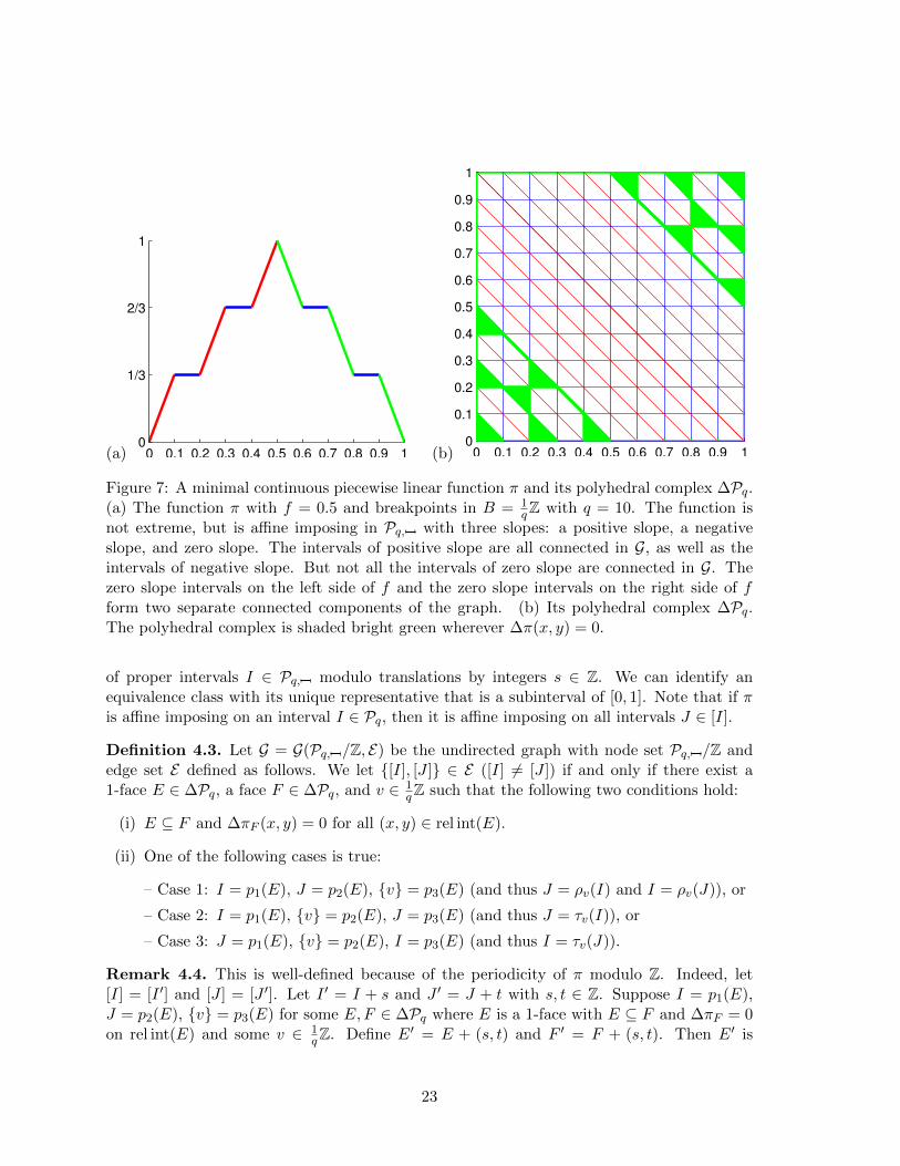
Figure 7: A minimal continuous piecewise linear function π and its polyhedral complex ∆Pq.(a) The function π with f = 0.5 and breakpoints in B = 1

qZ with q = 10. The function isnot extreme, but is affine imposing in Pq, with three slopes: a positive slope, a negativeslope, and zero slope. The intervals of positive slope are all connected in G, as well as theintervals of negative slope. But not all the intervals of zero slope are connected in G. Thezero slope intervals on the left side of f and the zero slope intervals on the right side of fform two separate connected components of the graph. (b) Its polyhedral complex ∆Pq.The polyhedral complex is shaded bright green wherever ∆π(x, y) = 0.

of proper intervals I ∈ Pq, modulo translations by integers s ∈ Z. We can identify anequivalence class with its unique representative that is a subinterval of [0, 1]. Note that if πis affine imposing on an interval I ∈ Pq, then it is affine imposing on all intervals J ∈ [I].

Definition 4.3. Let G = G(Pq, /Z, E) be the undirected graph with node set Pq, /Z andedge set E defined as follows. We let {[I], [J ]} ∈ E ([I] 6= [J ]) if and only if there exist a1-face E ∈ ∆Pq, a face F ∈ ∆Pq, and v ∈ 1

qZ such that the following two conditions hold:

(i) E ⊆ F and ∆πF (x, y) = 0 for all (x, y) ∈ rel int(E).

(ii) One of the following cases is true:

– Case 1: I = p1(E), J = p2(E), {v} = p3(E) (and thus J = ρv(I) and I = ρv(J)), or

– Case 2: I = p1(E), {v} = p2(E), J = p3(E) (and thus J = τv(I)), or

– Case 3: J = p1(E), {v} = p2(E), I = p3(E) (and thus I = τv(J)).

Remark 4.4. This is well-defined because of the periodicity of π modulo Z. Indeed, let[I] = [I ′] and [J ] = [J ′]. Let I ′ = I + s and J ′ = J + t with s, t ∈ Z. Suppose I = p1(E),J = p2(E), {v} = p3(E) for some E,F ∈ ∆Pq where E is a 1-face with E ⊆ F and ∆πF = 0on rel int(E) and some v ∈ 1

qZ. Define E′ = E + (s, t) and F ′ = F + (s, t). Then E′ is

23

another 1-face in ∆Pq, F ′ is a face in ∆Pq with E′ ⊆ F ′ and ∆πF ′ = 0 on rel int(E′) andI ′ = I + s = p1(E

′), J ′ = J + t = p2(E′), and {v′} = p3(E

′), where v′ = v + s+ t ∈ 1qZ.

On the other hand, suppose, without loss of generality, I = p1(E), {v} = p2(E), J = p3(E)for some 1-face E ∈ ∆Pq contained in a face F ∈ ∆Pq with ∆πF = 0 on rel int(E) and somev ∈ 1

qZ. Define E′ = E+ (s, t− s) and F ′ = F + (s, t− s). Then E′ is another 1-face in ∆Pq,which is contained in the face F ′ ∈ ∆Pq, and ∆πF ′ = 0 on rel int(E′) with I ′ = I+s = p1(E

′),{v′} = p2(E

′), J ′ = J + t = p3(E′), where v′ = v − s+ t.

Lemma 4.5. Let π1, π2 be valid functions such that π = 12(π1 + π2). For θ = π, π1, or π2, if

θ is affine in int(I), and {[I], [J ]} ∈ E, then θ is affine in int(J) as well with the same slope.

Proof. Since θ is affine in int(I), let c, b ∈ R such that θ(x) = cx + b for x ∈ int(I). If{[I], [J ]} ∈ E , then one of three cases could happen.Case 1. I = p1(E), J = ρa(I) = p2(E), {a} = p3(E) for some 1-face E ∈ ∆Pq contained ina face F ∈ ∆Pq with ∆πF = 0 on rel int(E) and some a ∈ 1

qZ.If E = F , then for all v ∈ int(J), (a − v, v) ∈ rel int(E) = rel int(F ) and thus 0 =

∆πF (a−v, v) = ∆π(a−v, v) = π(a−v)+π(v)−π(a) = 0. Then, by Lemma 1.6, ∆θ(a−v, v) =θ(a− v) + θ(v)− θ(a) = 0 for all v ∈ int(J). Since a− v = ρa(v) ∈ int(I) for all v ∈ int(J),θ(a− v) = c(a− v) + b for all v ∈ int(J). Then θ(v) = −θ(a− v) + θ(a) = cv − ca− b+ θ(a)for v ∈ int(J), and therefore θ is affine in int(J) with the same slope.

On the other hand, if E ( F , then F is a 2-face (triangle) whose diagonal edge is E. Let{a} ( K = p3(F ). For all v ∈ int(J), (a− v, v) ∈ F and thus by Lemma 2.7,

lim(x,y)→(a−v,v)(x,y)∈rel int(F )

∆θ(x, y) = lim(x,y)→(a−v,v)(x,y)∈rel int(F )

(θ(x) + θ(y)− θ(x+ y)

)= 0. (11)

Let v ∈ int(J). Because v ∈ int(J), the set

Zv = { z | (z − v, v) ∈ rel int(F ) } = int(K) ∩ (int(I) + v)

is a open subinterval of K with a on its boundary. Thus we can specialize the limit (11) tothe points (x, y) = (z − v, v) with z ∈ Zv,

limz→az∈Zv

(θ(z − v) + θ(v)− θ(z)

)= 0. (12)

But since a− v ∈ int(I), θ is continuous at a− v, and so

limz→az∈Zv

θ(z − v) = θ(a− v).

Since also θ(v) does not depend on z, we find that the limit of θ(z) exists and equals

limz→az∈Zv

θ(z) = θ(a− v) + θ(v). (13)

We claim that the limit (13) is independent of the choice of v ∈ int(J). Indeed, let v′ ∈ int(J),then Zv, Zv′ , and Zv∩Zv′ are open (nonempty) subintervals of K with a on their boundaries,and thus

limz→az∈Zv

θ(z) = limz→a

z∈Zv∩Zv′

θ(z) = limz→az∈Zv′

θ(z).

24

Let L denote this limit. Then (13) implies θ(v) = −θ(a − v) + L = cv − ca − b + L forv ∈ int(J), and therefore θ is affine in int(J) with the same slope.

Case 2. I = p1(E), {a} = p2(E), J = τa(I) = p3(E) for some 1-face E ∈ ∆Pq containedin a face F ∈ ∆Pq with ∆πF = 0 on rel int(E) and some a ∈ 1

qZ. For brevity, we onlyprove the case where E = F . Then π(w − a) + π(a) = π(w) and thus, by Lemma 1.6,θ(w − a) + θ(a) = θ(w) for all w ∈ int(J). Again, since w − a = τ−1a (w) ∈ int(I) forall w ∈ int(J), we have θ(w − a) = c(w − a) + b for all w ∈ int(J). Then we obtainθ(w) = cw − ca + b + θ(a) for w ∈ int(J), and therefore θ is affine in int(J) with the sameslope.Case 3. J = p1(E), {a} = p2(E), I = τa(J) = p3(E) for some 1-face E ∈ ∆Pq contained ina face F ∈ ∆Pq with ∆πF = 0 on rel int(E) and some a ∈ 1

qZ. For brevity, we only prove thecase where E = F . Then π(u)+π(a) = π(u+a) and thus, by Lemma 1.6, θ(u)+θ(a) = θ(u+a)for all u ∈ int(J). Since u+a = τa(u) ∈ int(I) for all u ∈ int(J), we have θ(u+a) = c(u+a)+bfor all u ∈ int(J). Then we obtain θ(u) = θ(u+ a)− θ(a) = cu+ ca+ b− θ(a) for u ∈ int(J),and therefore θ is affine in int(J) with the same slope.

Intervals connected to covered intervals. For each I ∈ Pq, , let GI be the connectedcomponent of G containing [I]. We now define the set of all intervals connected to coveredintervals in the graph G,

S2q, ={J ∈ Pq,

∣∣ [J ] ∈ GI for some I ∈ P2q,

}.

This is a set of intervals on which π is affine imposing. (Actually, we will see below that it isexactly the set of intervals on which π is affine imposing; this will follow from Lemma 4.8.)

Theorem 4.6. π is affine imposing on S2q, . Moreover, let π1, π2 be valid functions such

that π = 12(π1 + π2). Then, for θ = π, π1, π2 and for each interval I ∈ S2q, , the function θ

is affine in int(J) with the same slope for every interval J ∈ GI .

Proof. From Lemma 4.5, it follows that if π is affine imposing in I and {[I], [J ]} ∈ E , then πis affine imposing in J . Let J ∈ S2q, . Then J must be in a connected component containingan interval I ∈ P2

q, . By induction on the length of a path between [I] and [J ] in G, π is affineimposing in each interval whose equivalence class is a node of the connected component GI ,and therefore is affine imposing in J . We conclude that π is affine imposing in S2q, . It followsdirectly from Lemma 4.5 that for each interval I ∈ S2q, , θ has the same slope in J for everyinterval J ∈ GI and θ = π, π1, π2.

Corollary 4.7. Suppose S2q, = Pq, . Then π is affine imposing in Pq, .

The function in Figure 7 illustrates how intervals can be connected in G and that intervalson which π has the same slope are not necessarily connected.

4.2 Non-extremality by equivariant perturbation

In this subsection, we will prove the following result.

Lemma 4.8. If S2q, 6= Pq, , then π is not extreme.

25

Proof. Let I ∈ Pq, \S2q, . This is an interval for which π is not known to be affine imposing.Consider the set

R =⋃

J∈Pq,

[J ]∈GI

int(J),

a union over all intervals whose equivalence classes are connected to [I] in the graph G. Notethat π is not known to be affine imposing over any of these intervals J . Indeed we will showthat we can perturb the function π simultaneously over all these intervals using a piecewiselinear function with breakpoints in 1

4qZ.To this end, let ψ be the Γ-equivariant function of Lemma 2.16. This is a continuous

piecewise linear function with breakpoints in 14qZ, which is zero on all of the breakpoints in

12qZ. Let π = δR · ψ where δR is the indicator function for the set R. By multiplying withthe indicator function, we restrict the Γ-equivariant function to the set R; outside of R, theresulting function π is zero. Because the boundary of R consists of breakpoints in 1

qZ, whereψ is zero, the function π is continuous. Let

ε = min{

∆πF (x, y) 6= 0∣∣∣ F ∈ ∆P 1

4qZ, F ⊆ [0, 1]2, (x, y) ∈ vert(F )

}.

Note that ε is well-defined and positive because it is a minimum over a finite number ofpositive numbers. Here we consider π as a piecewise linear function with breakpoints in 1

4qZand use the fact that π is subadditive. We will show that for

π1 = π + ε3 π, π2 = π − ε

3 π,

that π1, π2 are minimal valid functions, and hence π is not extreme. We will show this justfor π1 as the proof for π2 is the same.

First, observe that π1 is periodic modulo Z.Also, since ψ(0) = 0 and ψ(f) = 0, we see that π1(0) = 0 and π1(f) = 1.We want to show that π1 is symmetric and subadditive. We will do this by analyzing

the function ∆π1(x, y) = π1(x) + π1(y) − π1(x + y) and showing that ∆π1(x, y) ≥ 0 for allx, y ∈ R. Since ψ is piecewise linear over 1

4qZ, π1 is also piecewise linear with breakpoints

in 14qZ. By Theorem 2.5, we only need to check ∆π1(x, y) ≥ 0 for all vertices (x, y) of the

complex ∆P4q.Let I , J , K ∈ P4q, ∪ P4q, , such that F = { (x, y) | x ∈ I , y ∈ J , x + y ∈ K } ∈ ∆P4q is

non-empty. Let ∆π1F

(u, v) = π1I(u) + π1

J(v)− π1

K(u+ v). Let (u, v) ∈ vert(F ).

In the following, we consider two cases: If ∆πF (u, v) > 0 (strict subadditivity), we makeuse of our choice of ε to show that ∆π1

F(u, v) ≥ 0. On the other hand, if ∆πF (u, v) = 0

(additivity), we show that ∆π1F

(u, v) = 0. This will prove two things. First, ∆π1(x, y) ≥ 0

for all x, y ∈ R, and therefore π1 is subadditive. Second, since π is symmetric, if F ⊂ { (x, y) |x + y ≡ f (mod 1) }, then ∆πF (x, y) = 0 for all (x, y) ∈ vert(F ), which would imply that

∆π1F

(x, y) = 0 for all (x, y) ∈ vert(F ), proving that π1 is symmetric.

Strictly subadditive case. First, if ∆πF (u, v) > 0, then ∆πF (u, v) ≥ ε. Therefore, since|π| ≤ 1,

∆π1F

(u, v) ≥ πI(u)− ε/3 + πJ(v)− ε/3− πK(u+ v)− ε/3 = ∆πF (u, v)− ε ≥ 0.

26

(a)

0 1/4 1/2 3/4 10

2/51/23/5

1

(b)

34

14

116

34

24

0 116

14

1

1

0

24

R

R

Subcase 3b

Subcase 2

Subcase 1

Subcase 3a

Figure 8: Cases within the proof of Lemma 4.8 on a sample non-extreme function. (a) Thefunction π is piecewise linear on Pq = P4 with three slopes (red, blue, green solid lines).We construct the perturbed functions π1 (dashed lines) and π2 (dotted lines). (b) The two-dimensional complex ∆Pq = ∆P4 (thick black lines) and its refinement ∆P4q = ∆P16 (thinblack lines). The union R of open sets is the open interval (14 ,

12) in this example. The regions

of points (u, v) with u ∈ R (magenta), v ∈ R (yellow), or u+ v ∈ R (cyan) are shaded usingthe subtractive color model; thus we see the points with u, v ∈ R (red), u, u+ v ∈ R (blue),v, u + v ∈ R (green). In Subcase 1 (circles), u, v, u + v /∈ R (unshaded white regions). InSubcase 2 (squares), u, v ∈ 1

2qZ. In Subcase 3, we are not in Subcases 1 or 2; we showthat (u, v) lies in the relative interior of a 1-dimensional face F . In Subcase 3a (pentagons),F ⊂ { (x, y) | y = v } and v ∈ 1

qZ. In Subcase 3b (triangles), F ⊂ { (x, y) | x + y = u + v }and u+ v ∈ 1

qZ.

Additive case. Next, we will show that if ∆πF (u, v) = 0, then ∆π1F

(u, v) = 0. Supposethat ∆πF (u, v) = 0. We will proceed by cases. See Figure 8 for an illustration of these cases.

Subcase 1. Suppose u, v, u+ v /∈ R. Then δR(u) = δR(v) = δR(u+ v) = 0, and ∆π1F

(u, v) =∆πF (u, v) ≥ 0.

Subcase 2. Suppose u, v ∈ 12qZ. Then u+ v ∈ 1

2qZ and, by Lemma 2.16 (i), ψ(u) = ψ(v) =

ψ(u+ v) = 0. Thus ∆π1F

(u, v) = ∆πF (u, v) ≥ 0.

Subcase 3. Suppose we are not in subcases 1 or 2. That is, suppose ∆πF (u, v) = 0, notboth u, v are in 1

2qZ, and at least one of u, v, u+ v is in R. Since ∆π1(x, y) is symmetric in xand y, without loss of generality, since not both u, v are in 1

2qZ, we will assume that u /∈ 12qZ.

There exists a unique face F ∈ ∆Pq with rel int(F ) ⊆ rel int(F ). Then ∆πF (x, y) =∆π(x, y) = ∆πF (x, y) for all (x, y) ∈ rel int(F ). This implies ∆πF (x, y) = ∆πF (x, y) for all

(x, y) ∈ F . There is a unique face E ∈ ∆Pq with E ⊆ F and (u, v) ∈ rel int(E). Sinceu /∈ 1

2qZ, (u, v) /∈ vert(∆Pq), and thus E is 1-dimensional or 2-dimensional. Since π issubadditive, ∆πF (x, y) = ∆π(x, y) ≥ 0 for all (x, y) ∈ rel int(F ), and thus ∆πF (x, y) ≥ 0 forall (x, y) ∈ F . Now since the affine function ∆πF equals 0 at the point (u, v) ∈ rel int(E) ⊆ F ,

27

we have∆πF (x, y) = 0 for all (x, y) ∈ rel int(E).

If E were a 2-dimensional face, then u ∈ int(I), v ∈ int(J), and u + v ∈ int(K) for someI, J,K ∈ P2

q, , thus u, v, u + v /∈ R, which is subcase 1. Therefore, we can assume thatE ∈ ∆Pq is a 1-dimensional face and hence a subset of one of the three following hyperplanes:x = u, y = v, or x+ y = u+ v.

Since u /∈ 12qZ ⊃

1qZ, E cannot be a subset of x = u because it is not a defining hyperplane

of the polyhedral complex ∆Pq. Observe that for any x ∈ R with x /∈ 1qZ, there is a unique

Ix ∈ Pq, such that x ∈ int(Ix). Since u /∈ 1qZ, there exists a unique interval Iu ∈ Pq, such

that u ∈ int(Iu). There are two possible subcases.

Subcase 3a. E ⊂ { (x, y) | y = v } and v ∈ 1qZ.

Since v ∈ 1qZ, u /∈

12qZ, it follows that u+ v /∈ 1

qZ, and there is a unique interval Iu+v ∈ Pq,containing u+ v in its interior. Then p1(E) = Iu, p2(E) = {v}, and p3(E) = τv(Iu) = Iu+v,and ∆πF (x, y) = 0 for (x, y) ∈ rel int(E). Therefore, by Definition 4.3, {[Iu], [Iu+v]} ∈ E andδR(u) = δR(u + v). Since v ∈ 1

qZ, we have ψ(v) = 0 and ψ(u) = ψ(τv(u)) = ψ(u + v) byLemma 2.16 (iii). It follows that ∆π(u, v) = π(u) + π(v)− π(u+ v) = 0, and therefore, sinceπ is continuous, ∆π1

F(u, v) = ∆πF (u, v) + ∆π(u, v) = ∆πF (u, v) = 0.

Subcase 3b. E ⊂ { (x, y) | x+ y = u+ v } and u+ v ∈ 1qZ.

Since u + v ∈ 1qZ, u /∈ 1

2qZ, it follows that v /∈ 1qZ, and there is a unique interval Iv ∈ Pq,

containing v in its interior. Then p1(E) = Iu, p2(E) = ρu+v(Iu) = Iv, p3(E) = {u + v},and ∆πF (x, y) = 0 for (x, y) ∈ rel int(E). Therefore, by Definition 4.3, {[Iu], [Iv]} ∈ E andδR(u) = δR(v). Since u + v ∈ 1

qZ, we have ψ(u + v) = 0 and ψ(u) = −ψ(ρu+v(u)) = −ψ(v)by Lemma 2.16 (ii). It follows that ∆π(u, v) = π(u) + π(v) − π(u + v) = 0, and therefore,since π is continuous, ∆π1

F(u, v) = ∆πF (u, v) + ∆π(u, v) = ∆πF (u, v) = 0.

We conclude that π1 (and similarly π2) is subadditive and symmetric, and therefore byTheorem 2.5 minimal and hence valid. Therefore π is not extreme.

Remark 4.9. To show that π is not extreme in the above lemma, the perturbation functionψ need not be piecewise linear. This choice was made to simplify the proof. In fact, anyΓ-equivariant function ψ 6= 0 constructed with Lemma 2.14 with |ψ| < |ψ| suffices. CompareFigures 4 and 5.

However, the specific form of our function ψ as a piecewise linear function with breakpointsin 1

4qZ (Lemma 2.16 (iv)) implies the following corollary.

Corollary 4.10. If π is not affine imposing over Pq, , then there exist distinct minimalπ1, π2 that are piecewise linear with breakpoints in 1

4qZ such that π = 12(π1 + π2).

Proof. By Corollary 4.7 and Lemma 4.8, we obtain that π is not extreme, and the proof ofLemma 4.8 chooses π1 and π2 as piecewise linear functions with breakpoints in 1

4qZ.

4.3 Extremality and non-extremality by a system of linear equations

Now we are able to prove that the finite system of linear equations, introduced in section 3,can decide extremality of π if the set B of breakpoints is chosen appropriately.

28

Theorem 4.11. Let π be a piecewise linear minimal valid function (possibly discontinuous)whose breakpoints are rational with least common denominator q. Then π is extreme if andonly if the system of equations (10) with B = 1

4qZ has a unique solution.

Proof. The forward direction is the contrapositive of Theorem 3.2, applied to the set ofbreakpoints B = 1

4qZ. For the reverse direction, we assume that the the system of equa-

tions (10) with B = 14qZ has a unique solution. Suppose that there exist distinct valid

functions π1, π2 that are piecewise linear with breakpoints in 14qZ such that π = 1

2(π1 + π2).

By Lemma 1.6, π1 and π2 are minimal. Then π1 and π2 are solutions to (10) with B = 14qZ,

a contradiction. Thus, by the contrapositive of Corollary 4.10, π is affine imposing in Pq, .Then π is also affine imposing on P4q, since it is a finer interval set. By Corollary 3.4, sinceπ is affine imposing in P4q, and the system of equations (10) with B = 1

4qZ has a uniquesolution, π is extreme.

4.4 Proofs of Theorems 1.3 and 1.5

We are now ready to present the proofs of Theorems 1.3 and 1.5.

Proof of Theorem 1.3. Given the piecewise linear function π, the algorithm performs thefollowing test. Test if the system (10) with B = 1

4qZ has a unique solution, where q is theleast common denominator of the breakpoints of π. If yes, then report that π is extreme; else,report that π is not extreme. Theorem 4.11 guarantees the correctness of this algorithm.

Finally, observe that the number of variables and constraints of system (10) is boundedpolynomially in q, and it can be written down and solved in a number of elementary operationsover the reals that is bounded by a polynomial in q.

Proof of Theorem 1.5. We first show that if π is extreme, then π| 14q

Z is extreme for

Rf ( 14qZ,Z). If not, then there exist two distinct minimal functions π1, π2, both functions

from 14qZ to R+, such that π| 1

4qZ = 1

2(π1 + π2). Let πi be the linear interpolation of πi,

i = 1, 2. It can be verified that πi is minimal because πi is minimal. This contradicts theextremality of π.

Now we show that if π| 14q

Z is extreme for Rf ( 14qZ,Z), then π is extreme. If π is not extreme

then by Theorem 4.11 the system of equations (10) does not have a unique solution. Thenwe can construct π1 and π2 as in the proof of Theorem 3.2 using the non-trivial elementin the kernel of (10), such that π = 1

2(π1 + π2). Since π is a continuous piecewise linearfunction, lim suph→0|

π(h)h | <∞. Theorem 2.9 then tells us that π1 and π2 both have to

be continuous, and by construction have breakpoints in 14qZ. Thus, since π1 6= π2, there

exists a breakpoint v ∈ 14qZ such that π1(v) 6= π2(v). Thus, π1| 1

4qZ and π2| 1

4qZ are two

distinct minimal valid functions for Rf ( 14qZ,Z). Moreover, since π = 1

2(π1 + π2), we have

that π| 14q

Z = 12

(π1| 1

4qZ + π2| 1

4qZ). This contradicts the extremality of π| 1

4qZ.

29

5 The irrational case: A new principle for proving extremality

In this section we investigate the properties of a family of piecewise linear continuous func-tions, periodic modulo Z, which we illustrate in Figure 9. Each of these functions has threeslopes, one of which is zero, and has translation points a0, a1, a2 such that π(ai) + π(x) =π(ai + x) for i = 0, 1, 2 and x in a certain interval [A,Ai]. When certain parameters arechosen appropriately, we will show that this function is extreme. In doing so, we showcase anew type of proof for a function to be extreme.

5.1 Function requirements

Here we explain restrictions that we require of some of the breakpoints of our function; seealso Figure 10.

Assumption 5.1. Let a0, a1, a2, t1, t2, f, A,A0, A1, A2 ∈ (0, 1) such that the following hold:

(i) The numbers t1, t2 are linearly independent over Q.

(ii) We have a1 = a0 + t1, a2 = a0 + t2, and 0 < a0 < a1 < a2 < A < f/2,

(iii) We have ai +A = f −Ai for i = 0, 1, 2, and A0 > A1 > A2 ≥ A0+A2 > A ≥ 0.

Let x0 be the midpoint of [A,A0], that is, x0 = (A+A0)/2. Observe that, for i = 1, 2,

ti = ai − a0 = A0 −Ai < A0 −A0 +A

2=A0 −A

2.

We then have x0 ± ti ∈ [A,A0] for i = 1, 2.

Let Γ = 〈ρf , τa0 , τa1 , τa2〉, as defined in section 2.5, and consider the orbit

X = Γ(x0) = { γ(x0) | γ ∈ Γ }.

From Lemma 2.11, Γ = Γ+ o 〈ρf 〉 where Γ+ = 〈τa0 , τa1 , τa2〉 = 〈τa0 , τ−1a0 τa1 , τ

−1a0 τa2〉. Let

τa ∈ Γ+ be a translation and observe that

τa0(τa(x0)) = a0 + (x0 + a) = (a0 + x0) + a = (f − x0) + a = f − (x0 − a) = ρf (τ−1a (x0)).

Therefore, the translation τa0 is redundant in this orbit and we can rewrite X with one fewertranslation as X = { γ(x0) | γ ∈ 〈ρf , τ−1a0 τa1 , τ

−1a0 τa2〉 }, or more simply as

X = (x0 + Λ) ∪ (ρf (x0) + Λ)

where Λ = 〈t1, t2〉Z. The key element here is that Λ is dense in R because t1, t2 are linearlyindependent over Q.

For the same reason, there is bijection from x0 + Λ to Z2 as x0 + λ1t1 + λ2t2 7→ (λ1, λ2).Let ` : x0 + Λ → N by x 7→ |λ1| + |λ2|. This map is well defined because of the bijectionbetween x0 + Λ and Z2.

Recall now that if π is a minimal valid function and π = 12(π1 + π2) with valid func-

tions π1, π2, then by Lemma 1.6, π, π1, π2 are minimal as well. Furthermore, from Lemma 1.6,if π(x) + π(y) = π(x + y), then πi(x) + πi(y) = πi(x + y) for i = 1, 2. Thus the differenceπ = π1 − π satisfies also π(x) + π(y) = π(x+ y).

30

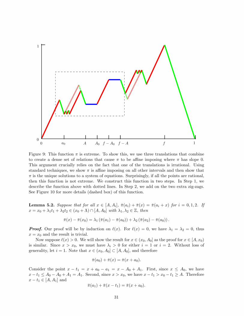
f −A0A0A00

f −A

1

1a0 f

Figure 9: This function π is extreme. To show this, we use three translations that combineto create a dense set of relations that cause π to be affine imposing where π has slope 0.This argument crucially relies on the fact that one of the translations is irrational. Usingstandard techniques, we show π is affine imposing on all other intervals and then show thatπ is the unique solutions to a system of equations. Surprisingly, if all the points are rational,then this function is not extreme. We construct this function in two steps. In Step 1, wedescribe the function above with dotted lines. In Step 2, we add on the two extra zig-zags.See Figure 10 for more details (dashed box) of this function.

Lemma 5.2. Suppose that for all x ∈ [A,Ai], π(ai) + π(x) = π(ai + x) for i = 0, 1, 2. Ifx = x0 + λ1t1 + λ2t2 ∈ (x0 + Λ) ∩ [A,A0] with λ1, λ2 ∈ Z, then

π(x)− π(x0) = λ1 (π(a1)− π(a0)) + λ2 (π(a2)− π(a0)) .

Proof. Our proof will be by induction on `(x). For `(x) = 0, we have λ1 = λ2 = 0, thusx = x0 and the result is trivial.

Now suppose `(x) > 0. We will show the result for x ∈ (x0, A0] as the proof for x ∈ [A, x0)is similar. Since x > x0, we must have λi > 0 for either i = 1 or i = 2. Without loss ofgenerality, let i = 1. Note that x ∈ (x0, A0] ⊂ [A,A0], and therefore

π(a0) + π(x) = π(x+ a0).

Consider the point x − t1 = x + a0 − a1 = x − A0 + A1. First, since x ≤ A0, we havex− t1 ≤ A0 −A0 +A1 = A1. Second, since x > x0, we have x− t1 > x0 − t1 ≥ A. Thereforex− t1 ∈ [A,A1] and

π(a1) + π(x− t1) = π(x+ a0).

31

A1

A A0 f − A0 f − Ax0

τa1

x0 + t1

f2

ρf

τ−1a0

ρf

A2

a0 a2a1

Figure 10: A zoomed in picture of Figure 9 to show in further detail the variables discussedin this section. For our construction to work, we choose ai and f − ai, for either i = 1 ori = 2, to be irrational numbers, and all other breakpoints to be rational. It follows thatt1 = a1−a0 and t2 = a2−a0 are linearly independent over Q. The arrows indicate the actionof the translations τa1 , τ−1a0 and the reflection ρf .

Subtracting these two equations and rearranging terms yields

π(x)− π(x− t1) = π(a1)− π(a0).

Since x− t1 ∈ [A,A0] and `(x− t1) = |λ1−1|+ |λ2| = |λ1|−1 + |λ2| = `(x)−1, the inductionhypothesis holds for x− t1 and hence

π(x− t1)− π(x0) = (λ1 − 1)(π(a1)− π(a0)) + λ2(π(a2)− π(a0)).

Therefore

π(x)− π(x0) =(π(x)− π(x− t1)

)+(π(x− t1)− π(x0)

)=(π(a1)− π(a0)

)+((λ1 − 1)(π(a1)− π(a0)) + λ2(π(a2)− π(a0))

)= λ1 (π(a1)− π(a0)) + λ2 (π(a2)− π(a0)) .

As stated before, the proof for x ∈ [A, x0) is similar and is done by supposing λ1 < 0 andconsidering the point x+ a1 − a0 = x+ t1. The calculations are very similar.

32

5.2 Construction

We now give a precise definition of the function in Figure 9, and then apply the above lemma.This function will have three slopes, c1, c2, c3, where we choose c2 = 0. The construction willbe done in two steps. We leave this construction general because, although we will only showit is extreme for one choice of parameters, it is indeed extreme for many choices.

Step 1. We will determine variables dij , signifying the ith interval of slope cj . The intervalswritten in order have the following lengths:

d11, d13, d

21, d

23, d

12, d

31, d

22, d

33, d

41, d

43, d

51, 1− f,

where a0 = d11 + d13, A = a0 + d21 + d23, A0 = A + d12, and f − A0 = A + d12 + d31. Note thatthe interval [A,A0] has slope c2 = 0 in this notation.

We begin by picking f ∈ (0, 1). On the interval [f, 1], the function will have only slope c3.We divide up the length of the interval [0, f ] into lengths d1, d2, d3 that will be the amount of[0, f ] with slopes c1, c2, c3, respectively. So d1 + d2 + d3 = f . Therefore we have the followingequations:

c1 =1− d2c2 − d3c3

d1, c2 = 0, c3 =

−1

1− f, d1 + d2 + d3 = f.

Now we subdivide each of these lengths into smaller lengths. Inside [0, f ], we want 5 intervalswith slope c1, 2 intervals with slope c2 and 4 intervals with slope c3. Therefore we giveourselves the following positive variables

d11 + d21 + d31 + d41 + d51 = d1,

d12 + d22 = d2,

d13 + d23 + d33 + d43 = d3.

To preserve symmetry in the function, we restrict ourselves to

d11 = d51, d21 = d41, d12 = d22, d13 = d43, d23 = d33.

We choose our parameters such that

π(a0) + π(A) = π(f −A0) and a0 +A = f −A0,

which gives the two equations

d11 + d13 = d12 + d31, d11c1 + d13c3 = d12c2 + d31c1.

By choosing values for the variables f, d1, d2, and d11 + d13, the remaining variables can bedetermined uniquely.

Step 2. We will create 2 more additivity equations:

π(a1) + π(A) = π(a1 +A) and π(a2) + π(A) = π(A+ a2).

For this, we pick positive δ1, δ2 such that the sum of these values is less than d12/2. We sett1 = δ1, t2 = δ1 + δ2, a1 = a0 + t1 and a2 = a0 + t2. For each δi, find δi1, δ

i3 such that

33

δi1 + δi3 = δi and c1δi1 + c3δ

i3 = 0. With this, we force π(a0) = π(a1) = π(a2), and the desired

additivity relations follow.Now we adjust some previous parameters to make room for new zig-zags:

d21 = d21 − δ11 − δ21 , d41 = d41 − δ11 − δ21 , d23 = d23 − δ13 − δ23 , d33 = d33 − δ13 − δ23 .

Let e3 = 1− f . Now the intervals written in order have the following lengths:

d11, d13, δ

11 , δ

13 , δ

21 , δ

23 , d

21, d

23, d

12, d

31, d

22, d

33, d

41, δ

23 , δ

21 , δ

13 , δ

11 , d

43, d

51, e3,

where each interval has slope corresponding to the subscript. Let t1 = δ1, t2 = δ1 + δ2, andlet a1 = a0 + t1, a2 = a0 + t2. The parameters δ1, δ2 will be chosen such that t1, t2 are linearlyindependent over Q.

5.3 Proof of extremality in the irrational case

Theorem 5.3. Let f = 4/5, d1 = 3/5, d3 = 1/10, d11+d13 = 15/100, δ1 = 1/200, δ2 =√

2/200and let π be the function given by these parameters and the construction above. Then π isextreme.

Proof. Using Theorem 2.5, it can be shown that π is a minimal function. Furthermore,these parameters satisfy Assumption 5.1 and π satisfies the hypotheses of Lemma 5.2. Letπ1, π2 be minimal valid functions such that π = 1

2(π1 + π2). From Theorem 2.9, it followsthat π = π1 − π is continuous, and since π, π1, π2 are minimal, π(0) = 0.

Let I ∈ PB, be an interval with slope c1 and let x ∈ int(I). Since int(I) is open, thereexists an ε > 0 such that U = [x − ε/2, x + ε/2] ⊂ int(I) and V = [0, ε] ⊂ [0, d11]. Sinceπ(u) + π(v) = π(u + v) for all u ∈ U, v ∈ V , by the Interval Lemma, π is affine imposingin U, V, U + V , and π has the same slopes on U, V, U + V . Repeating this for every point xwhere π has slope c1 shows that π is affine imposing in all intervals where it has slope c1 andπ has the same slope, say c1, in these intervals. In other words, π′(x) = c1 for all x such thatπ′(x) = c1.

Similarly, we find that π is affine imposing in all intervals with slope c3, and the function πhas the same slopes in these intervals. Furthermore, since π has slope c3 on the interval [f, 1]and θ(f) = 1, θ(1) = 0 for θ = π, π1, the slope c3 is fixed for each function to c3 = −1

1−f .Therefore π′(x) = 0 for all x such that π′(x) = c3.

Since π is a continuous piecewise linear function and π(0) = 0, π(x) =∫ x0 π′(t) dt, where

the finitely many values of t where π′ does not exist are ignored. The following calculationsstem from the facts that π′(x) = 0 wherever π′(x) = c3 and that π′ on [0, a2] is either of slopec1 or c3. Therefore,

π(a1)− π(a0) = c1δ11 ,

π(a2)− π(a0) = c1(δ11 + δ21).

Note that δi1 = c3c3−c1 δ

i. Let α = c3c3−c1 . Let t1 = δ1 and t2 = δ1 + δ2. Then

π(a1)− π(a0) = c1αt1,

π(a2)− π(a0) = c1αt2.

34

Recall that [A,A0] is the first interval with slope c2 = 0 and let x ∈ (x0 + Λ) ∩ [A,A0].By Lemma 5.2, we have

π(x)− π(x0) = λ1(π(a1)− π(a0)) + λ2(π(a2)− π(a0))

= λ1c1αt1 + λ2c1αt2

= αc1(λ1t1 + λ2t2)

= αc1(x− x0).

That isπ(x) = π(x0) + αc1(x− x0)

and therefore, since Λ is dense in R, π(x) is affine on a dense set in [A,A0]. Since π iscontinuous and π is affine on all of [A,A0], the function π is affine imposing in [A,A0]. Since[A,A0] and f − [A,A0] are connected via the symmetry reflection, π is also affine imposingin f − [A,A0] and these intervals must have the same slope.

Since π is continuous with three slopes, we can set up a system of equations on threeslopes that is satisfied by π, π1, π2. We will demonstrate this system has a unique solutionusing just the equations π(f) = 1, π(1) = 0, and π(a0) +π(A) = π(f −A) where a0, A, f −Aare defined above. These equations yield the following system of equations, which is invariantwith respect to δ1, δ2: d1 d2 d3

d1 d2 d3 + e3d11 − d31 −d12 d13

c1c2c3

=

100

. (14)

Plugging the parameters into the system of equations, we have the matrix equation 3/5 1/10 1/103/5 1/10 3/10

2/15− 1/10 −1/20 1/60

c1c2c3

=

100

. (15)

This system has a unique solution, which is c1 = 5/2, c2 = 0, c3 = −5. Therefore, π = π1 = π2

and π is extreme.

5.4 Proof of non-extremality in the rational case

Theorem 5.4. Let f = 4/5, d1 = 3/5, d3 = 1/10, d11 + d13 = 15/100. Under the constructionabove, these values uniquely determine the values d11, d

13, d

21, d

23, d

12, d

31, d

22, d

33, d

41, d

43, d

51. Let 0 <

δ1, δ2 ∈ Q be any rational numbers such that δ1 + δ2 < d21 +d22 and let π be the function givenby these parameters and the construction above. Then π is not extreme.

Proof. Since the choice of δ1, δ2 does not affect the slope on the intervals, we know from theproof of Theorem 5.3 that the slopes of π are c1 = 5/2, c2 = 0, c3 = −5. By the construction,the function π takes slope c2 = 0 only on two intervals, [A,A0] and f − [A,A0], which aresymmetric about the point f/2. Between them is the interval [A0, f−A0] of length d31 = 1/10,on which π has slope c1 = 5/2. The midpoint of this interval is f/2. Since π satisfies thesymmetry condition, π(f/2) = 1/2. We thus find

π(x) =1

2− 1

2· 1

10· 5

2=

1

2− 1

8=

3

8for x ∈ [A,A0] (16a)

35

and

π(x) =1

2+

1

2· 1

10· 5

2=

1

2+

1

8=

5

8for x ∈ f − [A,A0] (16b)

as the values of π on the two slope-0 intervals.Since all the input parameters were chosen to be rational, there exists a number q ∈ Z+

such that the breakpoints of π are all in 1qZ. We consider the graph G = G(Pq, /Z, E)

introduced in section 4.1. By Lemma 4.5, if the equivalence classes [I], [J ] of two intervalsI, J ∈ Pq, are connected by a path in E , then π has the same slope on I and J . Let Z ⊆ Pq,be the set of all intervals where π has slope c2 = 0. Then, in particular, the intervals I ∈ Zare connected only to other intervals in Z.

Now we will show that none of the intervals in Z is covered, i.e., Z ∩ P2q, = ∅. Suppose

I ∈ Z is covered. By Lemma 4.1, there exists a two-dimensional face F ∈ ∆Pq with

∆π(x, y) = π(x) + π(y)− π(x+ y) = 0 for all (x, y) ∈ int(F ). (17)

such that I is one of the intervals I1 = p1(F ), I2 = p2(F ), or I3 = p3(F ), and π has the sameslope on I1, I2, I3. Thus π has slope 0 on I1, I2, I3. By (16), however, π(x), π(y), π(x+y) ≡ 1

8(mod 1

4) and thus ∆π(x, y) ≡ 18 (mod 1

4) for (x, y) ∈ rel int(F ). This is a contradictionto (17).

Thus we have showed that none of the equivalence classes of the intervals in Z is connectedby a path in G to the equivalence class of a covered interval. Therefore S2q, 6= Pq, . Hence,by Lemma 4.8, π is not extreme.

Theorems 5.3 and 5.4 show that a piecewise linear function with irrational breakpointscan be extreme, even if any nearby piecewise linear function with rational breakpoints is notextreme. This may suggest that an algorithm for deciding the extremality of functions withrational breakpoints that is oblivious to the sizes of the denominators of the breakpoints isnot possible.

References

[1] K. Andersen, Q. Louveaux, R. Weismantel, and L. Wolsey, Inequalities from two rows ofa simplex tableau, Integer Programming and Combinatorial Optimization. 12th Interna-tional IPCO Conference, Ithaca, NY, USA, June 25–27, 2007. Proceedings (M. Fischettiand D. Williamson, eds.), Lecture Notes in Computer Science, vol. 4513, Springer Berlin/ Heidelberg, 2007, pp. 1–15, doi:10.1007/978-3-540-72792-7_1.

[2] K. Andersen, C. Wagner, and R. Weismantel, On an analysis of the strength of mixed-integer cutting planes from multiple simplex tableau rows, SIAM Journal on Optimization20 (2009), no. 2, 967–982.

[3] A. Atamturk and K. Kianfar, n-step mingling inequalities: new facets for the mixed-integer knapsack set, Mathematical Programming 132 (2012), no. 1–2, 79–98, doi:

10.1007/s10107-010-0382-6.

36

[4] E. Balas, Intersection cuts – a new type of cutting planes for integer programming,Operations Research 19 (1971), 19–39.

[5] E. Balas, S. Ceria, G. Cornuejols, and N. R. Natraj, Gomory cuts revisited, OperationsResearch Letters 19 (1996), no. 1, 1–9, MR 97d:90059.

[6] A. Basu, P. Bonami, G. Cornuejols, and F. Margot, On the relative strength of split,triangle and quadrilateral cuts, Mathematical Programming Ser. A 126 (2009), 281–314,doi:10.1007/s10107-009-0281-x.

[7] A. Basu, M. Conforti, G. Cornuejols, and G. Zambelli, Maximal lattice-free convex setsin linear subspaces, Mathematics of Operations Research 35 (2010), 704–720.

[8] , Minimal inequalities for an infinite relaxation of integer programs, SIAM J.Discret. Math. 24 (2010), 158–168, doi:10.1137/090756375.

[9] , A counterexample to a conjecture of Gomory and Johnson, Mathematical Pro-gramming Ser. A 133 (2012), 25–38.

[10] A. Basu, R. Hildebrand, and M. Koppe, Equivariant perturbation in Gomory and John-son’s infinite group problem. II. The unimodular two-dimensional case, Integer Program-ming and Combinatorial Optimization (M. Goemans and J. Correa, eds.), Lecture Notesin Computer Science, vol. 7801, Springer, 2013, pp. 62–73, ISBN 978-3-642-36693-2.

[11] , Equivariant perturbation in Gomory and Johnson’s infinite group problem. III.Foundations for the k-dimensional case and applications to k = 2, eprint arXiv:1403.4628[math.OC], 2014.

[12] , Equivariant perturbation in Gomory and Johnson’s infinite group problem. IV.The general unimodular two-dimensional case, Manuscript, 2014.

[13] A. Basu, R. Hildebrand, M. Koppe, and M. Molinaro, A (k + 1)-slope theorem for thek-dimensional infinite group relaxation, SIAM Journal on Optimization 23 (2013), no. 2,1021–1040, doi:10.1137/110848608.

[14] V. Borozan and G. Cornuejols, Minimal valid inequalities for integer constraints, Math-ematics of Operations Research 34 (2009), 538–546, doi:10.1287/moor.1080.0370.

[15] M. Conforti, G. Cornuejols, and G. Zambelli, Corner polyhedra and intersection cuts,Surveys in Operations Research and Management Science 16 (2011), 105–120.

[16] G. Cornuejols and F. Margot, On the facets of mixed integer programs with two integervariables and two constraints, Mathematical Programming 120 (2009), 429–456, doi:10.1007/s10107-008-0221-1.

[17] G. Cornuejols and M. Molinaro, A 3-Slope Theorem for the infinite relaxation in theplane, Mathematical Programming 142 (2013), no. 1–2, 83–105, doi:10.1007/s10107-012-0562-7.

37

[18] S. S. Dey and J.-P. P. Richard, Facets of two-dimensional infinite group problems, Math-ematics of Operations Research 33 (2008), no. 1, 140–166, doi:10.1287/moor.1070.0283.

[19] , Relations between facets of low- and high-dimensional group problems, Mathe-matical Programming 123 (2010), no. 2, 285–313, doi:10.1007/s10107-009-0303-8.

[20] S. S. Dey, J.-P. P. Richard, Y. Li, and L. A. Miller, On the extreme inequalities ofinfinite group problems, Mathematical Programming 121 (2009), no. 1, 145–170, doi:10.1007/s10107-008-0229-6.

[21] R. E. Gomory, Some polyhedra related to combinatorial problems, Linear Algebra and itsApplications 2(4) (1969), 451–558.

[22] R. E. Gomory and E. L. Johnson, Some continuous functions related to corner polyhedra,I, Mathematical Programming 3 (1972), 23–85, doi:10.1007/BF01585008.

[23] , Some continuous functions related to corner polyhedra, II, Mathematical Pro-gramming 3 (1972), 359–389, doi:10.1007/BF01585008.

[24] , T-space and cutting planes, Mathematical Programming 96 (2003), 341–375,doi:10.1007/s10107-003-0389-3.

[25] M. Hall, The theory of groups, AMS Chelsea Publishing Series, American MathematicalSociety, 1976, ISBN 9780821819678.

[26] K. Kianfar and Y. Fathi, Generalized mixed integer rounding inequalities: facets forinfinite group polyhedra, Mathematical Programming 120 (2009), 313–346.

[27] , Generating facets for finite master cyclic group polyhedra using n-step mixedinteger rounding functions, European Journal of Operational Research 207 (2010), 105–109.

[28] Q. Louveaux and L. Poirrier, An algorithm for the separation of two-row cuts, Mathemat-ical Programming 143 (2014), no. 1–2, 111–146, doi:10.1007/s10107-012-0597-9.

[29] L. A. Miller, Y. Li, and J.-P. P. Richard, New inequalities for finite and infinite groupproblems from approximate lifting, Naval Research Logistics (NRL) 55 (2008), no. 2,172–191, doi:10.1002/nav.20275.

[30] J.-P. P. Richard, Y. Li, and L. A. Miller, Valid inequalities for MIPs and group polyhedrafrom approximate liftings, Mathematical Programming 118 (2009), no. 2, 253–277, doi:10.1007/s10107-007-0190-9.

38