IEEE TRANSACTIONS ON VEHICULAR TECHNOLOGY, VOL. 61, NO. 4, MAY 2012 1515

Equivalent Circuit Derivation and PerformanceAnalysis of a Single-Sided Linear Induction Motor

Based on the Winding Function TheoryWei Xu, Member, IEEE, Guangyong Sun, Member, IEEE, Guilin Wen,

Zhengwei Wu, Member, IEEE, and Paul K. Chu, Fellow, IEEE

Abstract—A linear metro that is propelled by a single-sidedlinear induction motor (SLIM) has recently attracted much atten-tion. Compared with the rotating-induction-machine drive system,the SLIM drive has advantages such as direct thrust withoutneeding friction between the wheel and the railway track, smallcross-sectional area, lack of gear box, and flexible line choice onaccount of the greater climbing capability and smaller turningcircle. However, due to its cut-open primary magnetic circuit,the SLIM has a longitudinal end effect and half-filled slots onthe primary ends, which can reduce the air-gap average fluxlinkage and thrust. Based on the winding function method, theSLIM is supposed to have the following three groups of windings:1) primary windings; 2) secondary fundamental windings; and3) secondary end effect windings. The proposed method considersthe actual winding distribution and structure dimensions. It cancalculate the mutual, self, and leakage inductance to describethe influence of the longitudinal end effect and half-filled slots.Moreover, a new equivalent model is presented to analyze thedifferent dynamic and steady-state performance. Comprehensivecomparisons between simulation and experimental results thatwere obtained from both one arc induction machine and one linearmetro indicate that the proposed model can be applied to predictthe SLIM performance and control scheme evaluation.

Index Terms—Arc induction machine, dynamic-state perfor-mance, equivalent circuit model, half-filled slots, linear metro, lon-gitudinal end effect, single-sided linear induction motor (SLIM),steady-state performance, winding function method.

Manuscript received March 17, 2011; revised July 23, 2011, September 25,2011, and November 23, 2011; accepted November 27, 2011. Date of pub-lication January 11, 2012; date of current version May 9, 2012. This workwas supported from in part by the National 973 Project of China under Grant2010CB328005, the Key Laboratory for Automotive Transportation Safety En-hancement Technology, Ministry of Communication of the People’s Republicof China, through the Open Fund under Grant CHD2011SY008, and the StateKey Laboratory of Vehicle NVH and Safety Technology through the Open Fundunder Grant NVHSKL-201002. The review of this paper was coordinated byDr. W. Zhuang.

W. Xu is with the State Key Laboratory of Advanced Design and Man-ufacture for Vehicle Body, Hunan University, Changsha 410082, China, andalso with the Platform Technologies Research Institute, RMIT University,Melbourne, VIC 3001, Australia (e-mail: weixuforhappy@gmail.com).

G. Sun (corresponding author) and G. Wen are with State Key Laboratoryof Advanced Design and Manufacture for Vehicle Body, Hunan University,Changsha 410082, China (e-mail: sgy800@126.com; wenguilin@yahoo.com.cn).

Z. Wu and P. K. Chu are with the Department of Physics and Materi-als Science, City University of Hong Kong, Kowloon, Hong Kong (e-mail:wuzw@ustc.edu.cn; paul.chu@cityu.edu.hk).

Color versions of one or more of the figures in this paper are available onlineat http://ieeexplore.ieee.org.

Digital Object Identifier 10.1109/TVT.2012.2183626

NOMENCLATURE

α1 Length of the entry-end-effect wave penetration coef-ficient (in meters).

α2 Length of the exit-end-effect wave penetration coeffi-cient (in meters).

σ Secondary sheet conductivity (1/(Ω.m)).η Efficiency.μ0 Air permeability (in newtons per square ampere).ωe Angular frequency of the power supply (in rad per

second).ωr Angular frequency of the rotor (in rad per second).τ Pole pitch (in meters).τe Half-wave length of the end-effect wave (in meters).θs Angle between the primary and secondary fundamen-

tal currents (in rad).by Flux density along the y-axis direction (in tesla).ge Equivalent air-gap length (in meters).Iabc,s Primary winding phase current in the ABC-axis (in

amperes).iαβ,s Primary winding phase current in the αβ-axis (in

amperes).pin Input active power (in watts).pout Output active power (in watts).qin Input reactive power (in var).s Per-unit slip.v2 Motor operating speed (in meters per second).Fe Thrust (in newtons).G Goodness factor.Gsv Speed voltage coefficient matrix.Is Primary phase current (in amperes).Ire Secondary-phase equivalent eddy current (in

amperes).J1 Equivalent primary current sheet density (in amperes

per meter square).Kp Winding pitch factor.Kd Winding distribution factor.Llr Secondary leakage inductance (in henry).Lls Primary leakage inductance (in henry).Lm Mutual inductance (in henry).Na Number of primary series turns per phase.Nabc,s Primary winding distribution functions in the

ABC-axis.Nαβ,s Primary winding distribution functions in the αβ-axis.

0018-9545/$31.00 © 2012 IEEE

1516 IEEE TRANSACTIONS ON VEHICULAR TECHNOLOGY, VOL. 61, NO. 4, MAY 2012

Fig. 1. Simple vehicle system diagram that is propelled by the SLIM.

Nαβ,rs Secondary fundamental winding distribution func-tions in the αβ-axis.

Nαβ,re Secondary end-effect winding distribution functionsin the αβ-axis.

Nse Effective winding turns in series per phase.Rs Primary resistance (in ohms).Rr Secondary resistance (in ohms).

I. INTRODUCTION

CURRENTLY, more than 20 urban transportation linesthat are propelled by single-sided linear induction mo-

tors (SLIMs) are commercialized worldwide, e.g., the linearmetro in Japan, then Vancouver light train in Canada, and theGuangzhou subway line 4 [1], [2]. The typical SLIM drivesystem is shown in Fig. 1. It is shown that the SLIM hung belowthe redirector supplied by the inverter on the vehicle. The sec-ondary is flattened on the railway track, and it usually consistsof an aluminum sheet that is 5–10 mm thick and a 20-mm-thick back iron that acts as the return path for the magnetic flux[3]–[5]. Compared with rotary induction machine (RIM) drivesystems, the SLIM system has the following merits. First, itcan achieve direct propulsive thrust, independent of the frictionbetween the wheels and rail, and can safely be operated, even inrainy or snowy weather [6]–[8]. Second, it has a smaller turningradius for its special bogie technique, smaller cross-sectionalarea for its omission of a gear box, larger acceleration, andstronger climbing ability due to its direct electromagnetic force.Hence, it offers a flexible line choice and reduced constructioncost, which is particularly favorable for subway systems [9]–[11]. Third, it has lower noise and less maintenance without agear box because of the nonadherent driving. Hence, it is anattractive mode of transportation in large cities [12].

However, as the SLIM primary moves, a new flux is con-tinuously developed at the primary entrance side, whereas theair-gap flux quickly disappears on the exit side [13]–[15]. Aneddy current in a direction counter to the primary current will beinduced in the secondary sheet, and it correspondingly affectsthe air-gap flux profile along the longitudinal direction. Thisphenomenon is called the “longitudinal end effect.” It candecrease air-gap average flux linkage (mutual inductance) andincrease relevant copper loss as its speed goes up [16]–[18].

Due to extensive research, many papers are currently avail-able with regard to the SLIM longitudinal end-effect analysis

brought by the sudden generation and disappearance of theair-gap penetrating flux density. In [1] and [2], a single-phaseT-model equivalent circuit is proposed to make electromagneticdesign for SLIM and then study its steady performance. Basedon the 1-D numerical analysis and relevant experimental veri-fication, two coefficients are provided to describe the influenceof the longitudinal end effect on the mutual and the secondaryresistance. This method can be adopted in a wide-speed regionand with different air-gap lengths. However, it is not suitablefor studying the SLIM dynamic performance, such as the vectorcontrol or direct torque control algorithm, because it is only asteady-state equivalent circuit. In [4]–[6], one simple and usefulfunction f(Q) according to the hypothetical curve of the sec-ondary eddy-current average value and the energy conversionbalance theorem is presented. The function is affected by theSLIM speed, secondary resistance, secondary inductance, andsome other structural parameters such as the primary length.For its simple equivalent model, it can easily be employedin different control algorithms similar to traditional inductionmachines. However, the function derivation is very coarse suchthat it is prone to increasing errors as the velocity goes up. In[7], steady- and dynamic-state performance by using the spaceharmonic method can theoretically be stimulated and the calcu-lated results have comparatively high accuracy. However, thismethod requires substantially more computing time, and theaccuracy mostly depends on many initially given parameters.If some key parameters are not rationally initialized, the finalsolution cannot be obtained due to nonconvergence. In [8], aFourier series expansion was used to describe the influence ofthe end effects of SLIM. However, the time to attain higheraccuracy in this technique can greatly increase for difficultdetermination of the mother wavelet. In [9], an equivalent pole-by-pole circuit model is derived from the viewpoint of primarywinding distribution. It is suitable for the steady and tran-sient performance analysis combined with different advancedcontrol algorithms. Simulation results are verified by severalexperiments. Unfortunately, one set of tenth-order differentialequations are needed to describe a basic model for a four-polemachine, and a higher order system of equations needs to beprovided as the pole number goes up. Furthermore, some coeffi-cients in this model mostly depend on experimental verificationand are difficult to directly extend to other structures.

In this paper, through the winding function method, a newmodel is presented to study both the steady- and the dynamic-state performance of SLIM. Using the primary winding distrib-ution, the longitudinal end effect and half-filled slots locatedin the primary ends are rationally taken into account in thewinding function expressions.

II. EQUIVALENT CIRCUITS OF THE SINGLE-SIDE

LINEAR INDUCTION MOTOR

According to Maxwell’s law, the air-gap flux density equa-tion of SLIM can be expressed by [17]

∂2by

∂x2− σμ0v2

∂by

∂x− jσμ0ωeby = −jμ0

π

τJ1e

j(ωet−πx/τ)

(1)

XU et al.: EQUIVALENT CIRCUIT DERIVATION AND PERFORMANCE OF SLIM BASED ON WINDING FUNCTION 1517

where σ is the secondary sheet conductivity, μ0 is the air per-meability, v2 is the primary operating speed, ωe is the angularspeed of the primary power supply, τ is the primary pole pitch,J1 is the equivalent primary current sheet density, and by isthe flux density along the y-axis direction. The solution ofby(x, t) is

by(x, t) =•

B0 e−j πxτ +

•B1 e−

xα1 e−j πx

τe +•

B2 ex

α2 ej πxτe (2)

where by consists of the following three parts: 1) B0; 2) B1;and 3) B2. B0 is the normal traveling wave, which travelsforward similar to the fundamental flux density in the RIM.B1 and B2, which are determined using boundary conditions,are the entrance- and exit-end-effect waves, respectively. α1 isthe penetration depth of the entry-end-effect wave, α2 is thepenetration depth of the exit-end-effect wave, and τe is the halfwavelength of the end-effect wave, which are functions of thespeed and motor structural parameters [19], [20].

Based on the air-gap flux density equation, the SLIM sec-ondary winding function is divided into the fundamental andend-effect components. First, it deduces the primary two-phasestationary axis model according to the primary actual windingdistribution. Because there are no obvious windings on thesecondary, the secondary winding function can be obtainedfrom the field distribution theory [21]. In theory, the secondarywinding function of the LIM consists of the following twoindependent components: 1) a fundamental part Nrs(x) and2) an end-effect part Nre(x). It supposes that two electricallyindependent but mutually coupled secondary windings can bederived from the steady and dynamic states of the air-gap mag-netic flux equations [22]. Moreover, it calculates all inductance,goodness factor, secondary resistance, and speed voltage coeffi-cients. Based on the energy conversion relationship between theprimary and the secondary [23], the mathematic expressions ofthrust, power factor, and efficiency are derived. Generally, thewhole derivation progress is quite complex, and more detailscan be found in [9] and [10]. A brief introduction on the theoryof winding function is given as follows.

The winding function N(x) of any winding is calculatedby counting conductors. One example is the simple single-turnwinding, as shown in Fig. 2(a). The conductors can be countedfrom left to right. If the current flows out of the paper, N(x) issupported to increase by one, and when the current flows intothe paper, N(x) can decrease by one. Hence, it is easy to get thecurve of N(x) in Fig. 2(b). Although the winding function is acircuit concept, it can be related to field quantities. If Ampere’slaw is applied to Fig. 2(a) along the path A1A2 A3A4A1,then ∮

H · dl = IN(x) (3)

where H is the flux intensity, and I is the total winding current.If the iron is supported infinitely permeable, H is zero, exceptin the air gap along path A3A4. Hence, the air-gap flux intensityH(x) can be described in terms of N(x) as

H(x) =IN(x)

ge(4)

Fig. 2. SLIM with arbitrary winding distribution.

Fig. 3. One-dimensional model of the SLIM.

where ge is the equivalent length of the air gap. Based on (4),the winding function N(x) is equivalent to the magnetic motiveforce IN(x) of the winding normalized by its current. Thus,it is independent of the machine excitation and relative to themachine geometry.

A brief summary of the expressions of three groups ofwinding functions is given as follows. The primary stationarythree-axis winding functions are [9]

⎧⎨⎩

Nas(x) = Nse

2 cos(πx/τ + π)Nbs(x) = Nse

2 cos(πx/τ + π/3)Ncs(x) = Nse

2 cos(πx/τ − π/3)(5)

where Nse = KpKdNa, Kp, and Kd are the winding pitchand distribution factors, respectively, and Na is the number ofprimary series turns per phase. Hence, Nse is called the effectivewinding turns in series per phase.

To obtain the stationary two-axis stator winding function ex-pressions Nαs and Nβs from the stationary three-axis windingdistributions, the following rules according to the theory of fluxlinkage balance should be obeyed by

Nas(x)ias+Nbs(x)ibs+Ncs(x)ics =Nαs(x)iαs+Nβs(x)iβs

(6)

where iαs and iβs can be achieved from ias, ibs, and icsby using static 3/2 coordination transformation. Hence, theprimary stationary two-axis winding functions are expressed by

{Nαs(x) = 3

4Nse sin(πx/τ)Nβs(x) = − 3

4Nse cos(πx/τ). (7)

The secondary winding functions, including both the funda-mental and end-effect parts, are abstract but can be obtainedfrom the electromagnetic relationship between the primary and

1518 IEEE TRANSACTIONS ON VEHICULAR TECHNOLOGY, VOL. 61, NO. 4, MAY 2012

the secondary [4]–[6]. The secondary fundamental winding

function•

Nrs is derived by

•Brs =

μ0

ge

•Nrs

•Irs (8)

where•

Brs and•

Irs are the secondary fundamental complex fluxdensity and secondary fundamental complex current, respec-

tively. Based on the air-gap flux density steady equation,•

Brs

can be expressed by

•Brs =

(3μ0/4ge)Nse√1 + (1/sG)2

Is exp [j(ωet − πx/τ + θs)] (9)

where s is the slip, G is the goodness factor, θs is the anglebetween the primary and secondary fundamental currents, Is

is the root-mean-square (RMS) value of the primary phasecurrent, and ωe is the angular frequency of the power supply.According to the 1-D model of the LIM depicted in Fig. 3[3], the secondary leakage inductance can be neglected for itssmaller value. Hence, the relationship between the primary andthe secondary current is described as

•Irs =

•Is

−jXm

jXm + Rr

s

=−Is√

1 + (1/sG)2exp [j(ωet + θs)]

(10)

where Xm and Rr are the mutual inductance reactance andsecondary resistance. Hence, based on (8)–(10), the secondary

fundamental winding functions•

Nrs are indicated by{Nαrs(x) = 3

4Nse sin(πx/τ)Nβrs(x) = − 3

4Nse cos(πx/τ). (11)

Similar to the solution of the secondary fundamental part,

the secondary end-effect part winding function•

Nre can be de-duced by

•Bre =

μ0

ge

•Nre

•Ire (12)

where•

Bre and•

Ire are the secondary end-effect complex fluxdensity and current, respectively. Based on the air-gap flux

density dynamic equation,•

Bre can be derived by [10], [19]

•Bre =

3μ04ge

NseIs

(1

α2+ sGπ

τ + j πτe

)(

1α1

+ 1α2

+ j 2πτe

)(1 + jsG)

× exp(−x/α1) exp[j

(ωet −

πx

τe

)]. (13)

There are three kinds of flux density waves in air gap, normalflux density wave, entry-end-effect flux density wave, and exit-end-effect flux density wave. α1 is the length of the entry-end-effect wave penetration coefficient, α2 is the length of theexit-end- effect wave penetration coefficient, and τe is the half-wave length of the end-effect wave. These three parameters canbring some influence on traveling distances of entry- and exit-end-effect flux density waves in the air gap [19]. With regard

to the normal traveling flux density, it is similar to the RIM,whose pitch is 2τ period, whereas the entry- and exit-end-effectwaves are brought by the end effect from the primary cut-openmagnetic paths (both entry and exit terminals), whose pitch are2τe period. Take the SLIM in the linear metro for example. α1

is 0.4 m, and α2 is 2 mm at a base speed of 40km/h; hence, theexit-end-effect wave more quickly attenuates than the entrance-end-effect wave. In general, τ (almost 0.25 m) is constant indifferent speed levels, whereas τe (about 0.1 m at the basespeed) is variable in different speed levels, which can quicklyincrease as the speed goes up [24].

Based on [3] and [8],•

Ire is

•Ire = K

11 + jsG

Is exp(jωet) (14)

where K is a function of the SLIM operation velocity, primarylength, and slip frequency. Based on (12)–(14), the secondary

end-effect winding function•

Nre is expressed as{

Nαre(x) = −N2K exp(−x/α2) sin(πx/τe − θe)

Nβre(x) = N2K exp(−x/α2) cos(πx/τe − θe)

(15)

where N2 and θe are related to the slip, goodness factor, andSLIM structural parameters, and they can be described as

N2 =

−3Nse

4

√(1

α2+ sGπ

τ

)2

+(

πτe

)2

√(1

α1+ 1

α2

)2

+(

πτe

)2

θe = tan−1πτe

1α2

+ sGπτ

− tan−1πτe

1α1

+ 1α2

.

According to aforementioned three groups of winding func-tion equations, it is interesting to see that the primary two-axisparts are the same as the secondary fundamental parts, whichare sinusoidal waves within the primary length. Because ofthe influence of the primary half-filled slots, the β-axis wavecan be regarded as lagging the α-axis by approximately π/2[9]. The secondary end-effect parts gradually attenuate fromthe entrance side to the exit side due to the influence of thelongitudinal end effect [25].

According to the fundamental theory of electrical machinery,the SLIM voltage equation is given in matrix form by

�u = [R]�i +d�λ

dt+ v2

π

τ[U ]�λ (16)

where several vectors are expressed as follows:

λ̄= [L]�i, �u=[uαs, uβs, 0, 0]T , �i=[iαs, iβs, iαr, iβr]T

[R]=

⎡⎢⎣

Rs 0 0 00 Rs 0 00 0 Rr 00 0 0 Rr

⎤⎥⎦ , [U ]=

⎡⎢⎣

0 0 0 00 0 0 00 0 0 10 0 −1 0

⎤⎥⎦

where L is an inductance matrix in which the element betweenany two winding functions mentioned in (7), (11), and (15) may

XU et al.: EQUIVALENT CIRCUIT DERIVATION AND PERFORMANCE OF SLIM BASED ON WINDING FUNCTION 1519

be calculated by

L12 =2μ0lδ3ge

pτ∫0

N1(x)N2(x)dx (17)

where N1(x) and N2(x) are two arbitrary winding functions,lδ is the primary stack width, and p is the number of primarypoles. There are 36 inductances to be calculated, and 18 ofthese inductances are independent of each other. Different fromthe RIM, the mutual inductance between the α- and the β-axessuch as Lαsβs is not zero, because its coupling results fromhalf-filled slots. The relationship between the flux linkage andcurrent in the two axes is (18), shown at the bottom of thepage, where Lls and Llr are the primary and secondary leakageinductance, respectively. Because of the influence of both half-filled slots and longitudinal end effect, the flux linkage in theα- or β-axis can be affected by the following four currentcomponents in the α- and β-axes:

• iαs;• iβs;• iαr;• iβr.

Inserting (18) into (16) and then making further simplifi-cation, two groups of voltage equations can be obtained asfollows. The voltage equations of the primary winding are{

uαs = Rsiαs + Llspiαs + Lmp(iαs + iαr) + eαt − eαst

uβs = Rsiβs + Llspiβs + Lmp(iβs + iβr) + eβt − eβst.(19)

The voltage equations of the secondary fundamentalwinding are{

0 = eαt + Lmp(iαs + iαr) + Llrpiαr + iαrRr + eαr

0 = eβt + Lmp(iβs + iβr) + Llrpiβr + iβrRr + eβr

(20)

where, in (19) and (20), eαt, eβt, eαst, and eβst are inducedvoltages, considering the influence by the longitudinal endeffects, and eαr and eβr are secondary moving voltages, whichare calculated by⎧⎪⎪⎪⎪⎨

⎪⎪⎪⎪⎩

eαt = p[L′

αsαreiαre + L′αsβreiβre

];

eβt = p[Lβsαrei

′αre + Lβsβrei

′βre

]eαst = −pLαsβsiβs; eβst = −pLαsβsiαs

eαr = v2(π/τ)λβr; eβr = −v2(π/τ)λαr

(21)

where p is the differential operator that is equal to d/dt.According to (19)–(21), the equivalent two-axis circuits areillustrated in Fig. 4. From (18). By neglecting the influence ofboth half-filled slots and longitudinal end effect, these mutualinductances between the α- and β-axes will become zero for the

Fig. 4. αβ-axis equivalent circuits of the actual SLIM with half-filled slotsand longitudinal end effect. (a) α-axis circuit. (b) β-axis circuit.

noncoupling relationship. Hence, the expression of flux linkagecan be simplified as

⎡⎢⎣

λαs

λβs

λαr

λβr

⎤⎥⎦=

⎡⎢⎣Lls+Lm 0 Lm 0

0 Lls+Lm 0 Lm

Lm 0 Llr+Lm 00 Lm 0 Llr+Lm

⎤⎥⎦⎡⎢⎣

iαs

iβs

iαr

iβr

⎤⎥⎦ .

(22)

Furthermore, the inducted and moving voltages eαt, eβt,eαst, eβst, eαr, and eβr can be rewritten as

⎧⎨⎩

eαt = 0; eβt = 0eαst = 0; eβst = 0eαr = ωrλβr; eβr = −ωrλαr

(23)

where ωr is the secondary electrical angular speed. The sim-plified equivalent circuits are indicated in Fig. 5. When thelongitudinal end effect and half-filled slots are ignored, i.e.,the SLIM totally appears as the RIM, the equivalent circuitsin Fig. 5 are similar to the traditional RIM. Different fromthe RIM, the special traits of the SLIM are the calculationof mutual and end-effect inductances that are functions of theslip, primary excitation frequency, and structure parameters.Moreover, the equivalent circuits in Fig. 5 can be extended todynamic coordinate references, and the derivation process andfinal equivalent circuits are similar to the RIM.

According to the energy conversion balance theorem be-tween the primary and the secondary, the thrust is de-scribed as

Fe = (3π/2τ)[i1]T [Gsv][i1] (24)

⎡⎢⎣

λαs

λβs

λαr

λβr

⎤⎥⎦ =

⎡⎢⎣

Lls + Lm + L′αsαre Lαsβs + L′

αsβre Lm + L′αsαre Lαsβr + L′

αsβre

Lαsβs + L′βsαre Lls + Lm + L′

βsβre Lβsαr + L′βsαre Lm + L′

βsβre

Lm + L′αrαre Lαrβs + L′

αrβre Llr + Lm + L′αrαre Lαrβr + L′

αrβre

Lβrαs + L′βrαre Lm + L′

βrβre Lβrαr + L′βrαre Llr + Lm + L′

βrβre

⎤⎥⎦

⎡⎢⎣

iαs

iβs

iαr

iβr

⎤⎥⎦ (18)

1520 IEEE TRANSACTIONS ON VEHICULAR TECHNOLOGY, VOL. 61, NO. 4, MAY 2012

Fig. 5. αβ-axis equivalent circuits of the ideal SLIM without the influences ofhalf-filled slots and longitudinal end effect. (a) α-axis circuit. (b) β-axis circuit.

where the matrix i1, including the end-effect part, is ex-pressed by

[i1] = [iαs, iβs, iαr, iβr, (iαs + iαr), (iβs + iβr)]T (25)

and matrix Gsv is the speed voltage coefficient matrix, whichmay be calculated similar to the inductance matrix L.

The input active power is

pin =32(uαsiαs + uβsiβs). (26)

The input reactive power is

qin =32(uβsiαs − uαsiβs). (27)

The output active power is

pout = (Fe − Fm)v2 (28)

where Fm is the total mechanical resistant force that involveswind and friction forces.

The power factor is

cos ϕ = pin/√

p2in + q2

in. (29)

The efficiency is

η = pout/pin. (30)

III. SIMULATION AND EXPERIMENTS

The aforementioned derivations describe the dynamic stateof the SLIM in differential linkage equations. The equationscan numerically be solved step by step by executing in theMATLAB/Simulink environment. In most dynamic cases, thestate variables include the secondary linkages and primarycurrents. The equations can also readily be used in the steady-state analysis by simply setting d/dt to jωe in (16). The fol-lowing two motors are analyzed in this paper, as illustrated inFigs. 6 and 7, respectively: 1) an arc induction motor (motor A)and 2) one SLIM applied in a linear metro train (motor B)[2], [17]. Their main dimensions and electrical parameters are

Fig. 6. Prototype of the arc induction motor (motor A).

Fig. 7. Arrangement of the SLIM and application on the train (motor B).(a) Primary. (b) Secondary. (c) Vehicle.

shown in Table I. The experimental method for deriving the fiveSLIM electrical parameters can be referred in [21]. Generallyspeaking, it is similar to the RIM in the following three steps:

Step 1) Direct-current (dc) phase resistance Rdc. An exactvalue of the primary dc phase resistance Rdc canbe obtained by measuring the dc voltage betweenwinding terminals and the dc that corresponds to therated alternating current (ac).

Step 2) Testing of open secondary circuit (decision on Rs,Lm, and Lls). The actual (ac excitation) the primaryphase winding resistance Rs, mutual inductance Lm,and primary leakage inductance Lls can be obtainedby disconnecting the secondary branch of the equiv-alent circuit.

Step 3) Testing of blocked secondary circuit (decision on Rr

and Llr). By performing the blocked secondary testwith the real reaction rail, the secondary resistanceRr and leakage inductance Llr can be obtained.

The testing analysis is combined with investigation by thenumerical circuit method and finite-element algorithm. Someunreasonable data should be neglected.

XU et al.: EQUIVALENT CIRCUIT DERIVATION AND PERFORMANCE OF SLIM BASED ON WINDING FUNCTION 1521

TABLE IMAIN DIMENSIONS AND PARAMETERS OF THE TWO MOTORS

As shown in Fig. 6, the arc induction machine prototypeexperimental bench has a rotor that is formed on the rim ofthe large-radius flywheel, whose primary is fed by a converter.The load cell is a dc machine that is connected to the shaftof the SLIM rig by belts. The dc machine can operate at anydesired speed and load below the rating values to provide differ-ent working points. The measurement sensors located betweenthe SLIM and the dc load can record the SLIM velocity, loadpower, and thrust.

Fig. 7 shows the structure of the primary, the secondary, andthe whole SLIM in the train. The primary is placed in the bogieunder the vehicle body, and the secondary sheet is flattened inthe experimental linear metro line.

A. Steady-State Simulation and Testing

Fig. 8 presents different thrust curves of two motors underconstant-current–constant-frequency excitation. As shown inthis figure, the maximal thrust of the SLIM, different fromthe RIM, will gradually decrease as the speed goes up by theinfluence of longitudinal end effects, particularly in the area ofhigh speed, whereas the RIM has constant maximal thrust indifferent frequencies for constant flux linkage in the air gap byits symmetry structure.

Fig. 8. Steady-state thrust curves with constant current and variable fre-quency. (a) Motor A under 11 A (real lines are the thrusts without endeffects, dashed lines the thrusts with end effects, and other shape lines are themeasured). (b) Motor B under 280 A (real lines are the thrusts without end effectand dashed lines the thrusts with end effects. All results are in simulation).

Fig. 9 shows the thrust excited by constant voltage in dif-ferent frequencies by the steady-state equations. In Fig. 9(a),it starts up under 220-V constant primary line voltage, and itscurrent is a little larger than the rating value for its smallerequivalent reactance. As the speed increases, the torque morequickly decreases than by the constant current in Fig. 8(a) for itsquicker air-gap flux attenuation. In general, the thrust predictionreasonably agrees with the measurement in various velocities.In Fig. 9(b), it is excited by the primary line voltage 530 V. Thegeneral trend of thrust is similar to Fig. 9(a).

The thrust of the SLIM applied in transportation is one of themost important indices. The actual SLIM control scheme oftenincludes the following two regions: 1) the “constant-current”region and 2) the “constant-power” region. Below the basespeed, the primary phase current and slip frequency are keptconstant. Because of the power conditioner voltage limitation,the constant-voltage operation is encountered above the basespeed. The phase current very quickly decreases due to theincreasing total impedance. To meet the drive system require-ment, it is necessary to linearly increase the slip frequency to

1522 IEEE TRANSACTIONS ON VEHICULAR TECHNOLOGY, VOL. 61, NO. 4, MAY 2012

Fig. 9. Steady-state thrust curves with constant voltage and variable fre-quency. (a) Motor A under 220-V line voltage (real lines are the thrusts withend effects, and other shape lines are the measured). (b) Motor B under 530-Vline voltage (all results are the thrusts with end effect in simulation).

prevent quick thrust reduction. Here, the steady-state drive per-formance of motor B in the overall working region is analyzedand compared with measurements, including the phase current,thrust, and efficiency curves, as shown in Fig. 10. The basespeed is 40 km/h. Simulation on the phase current, thrust, andefficiency is made according to the steady equations of theequivalent models. As shown in the figure, the simulated phasecurrent is close to the measurements. It is kept constant belowthe base speed and linearly decreases beyond the base speed.The thrust below the base speed decreases a little as the speedgoes up due to the end effect, although the phase current isconstant. Beyond the base point, the thrust linearly decreasesdue to the reducing phase current. The error in the base speedis obvious, because the control manner and slip frequency havebeen changed, but the efficiency calculation and measurementreasonably agree with each other.

B. Dynamic-State Simulation and Testing

Fig. 11 shows the thrust curves of motor B calculated bythe steady- and dynamic-state equations. In the entire range,the primary current is controlled to be constant at 280 A, and

Fig. 10. Simulated and measured performance curves in the whole operationrange.

Fig. 11. Thrust curves with constant current and frequency calculated at thesteady and dynamic states.

the primary frequency is supposed a constant at 10 Hz. It is ap-parent that the steady-state thrust is very close to the dynamic-state thrust in addition to the short starting-up procedure dueto the electromagnetic transition in the secondary. By the veri-fication of the steady-state model in Section III-A, it is shownthat the dynamic model is also reasonable to make performanceprediction. As shown in Fig. 11, it is interesting that thereare double-frequency (20-Hz) thrust ripples as the SLIM startsup. This case is due to the electromagnetic dynamics in thesecondary circuits produced by the longitudinal end effects.

Fig. 12 shows the constant-current start-up process, includingthe velocity, thrust, secondary fundamental, and eddy-currentcurves. In the overall operation region, the motor has a constantstator current of 280 A and a constant primary frequency of25 Hz. As shown in the figure, the secondary fundamental cur-rent, similar to the RIM, gradually decreases as the speed risesand is almost zero close to the synchronous point. However,the secondary end-effect part ascends with incremental speed,

XU et al.: EQUIVALENT CIRCUIT DERIVATION AND PERFORMANCE OF SLIM BASED ON WINDING FUNCTION 1523

Fig. 12. Constant-current start-up performance analysis. (a) Velocity. (b) Thrust. (c) Secondary fundamental current (RMS). (d) Secondary eddy current (RMS).

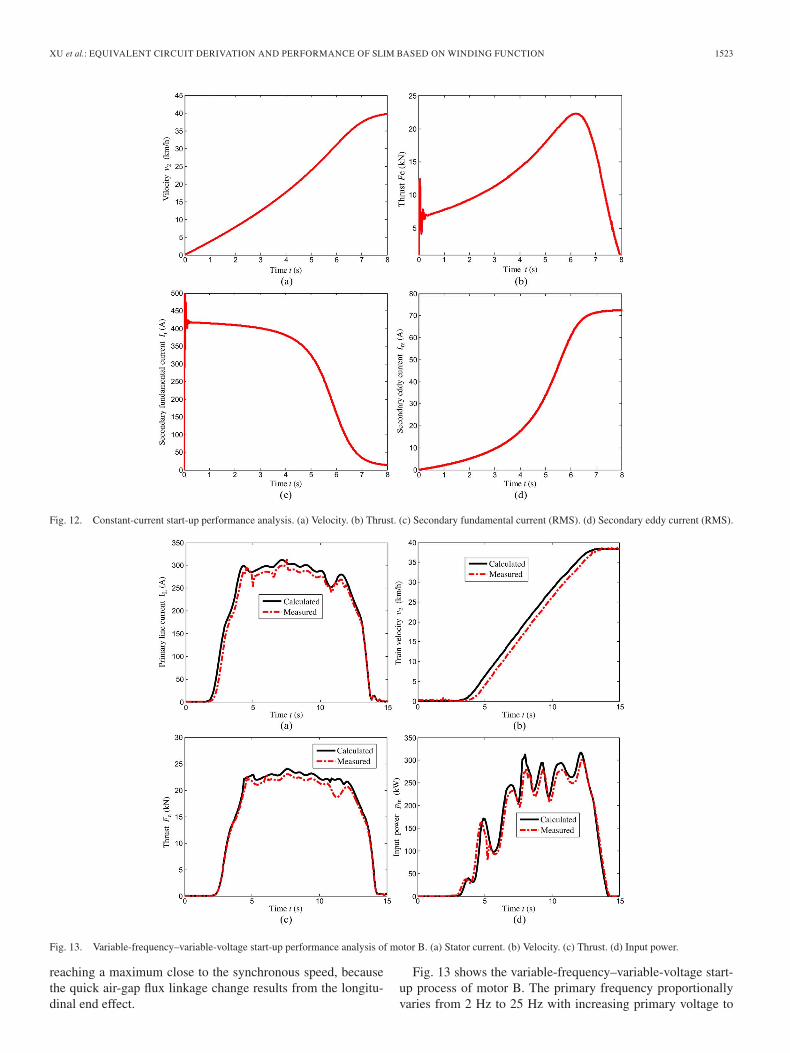
Fig. 13. Variable-frequency–variable-voltage start-up performance analysis of motor B. (a) Stator current. (b) Velocity. (c) Thrust. (d) Input power.

reaching a maximum close to the synchronous speed, becausethe quick air-gap flux linkage change results from the longitu-dinal end effect.

Fig. 13 shows the variable-frequency–variable-voltage start-up process of motor B. The primary frequency proportionallyvaries from 2 Hz to 25 Hz with increasing primary voltage to

1524 IEEE TRANSACTIONS ON VEHICULAR TECHNOLOGY, VOL. 61, NO. 4, MAY 2012

Fig. 14. Simple diagram of the indirect-rotor field-orientation controlalgorithm.

keep a comparatively constant air-gap flux linkage. The test iscarried out on the experimental linear metro line in cooperationwith a company, as illustrated in Fig. 7(c). During this testing,the primary two-phase voltages, two-phase currents, and op-erating speed are sampled by corresponding sensors and inputinto a Yokogawa DL750 oscillometric recorder. The samplingfrequency for voltage is about 20 kHz, and measured voltagedata can directly be input into the dynamic equations for step-by-step simulation. Some typical criteria by predication arecompared with their measurements, including the stator phasecurrent, train velocity, thrust, and input power. It is shown thatthe calculation agrees with the measurements in general.

To further verify the new model, the traditional indirect rotorfield control algorithm was executed on the arc induction motor(motor A). The flowchart of the control scheme is illustratedin Fig. 14, which includes the following three closed loops:1) rotor speed loop; 2) d-axis current loop; and 3) q-axis currentloop. These loops are modified by three proportional–integral(PI) regulators, which are similar to the RIM.

Fig. 15 shows the theoretical and measured curves of velocityv2 and thrust Fe. The velocity is given by 6.28 m/s, and thefield current is kept at a constant of 8 A in the whole process.The SLIM is accelerated from 0 m/s to 6.28 m/s in the first40 s, then operated with constant velocity for 20 s, and finallydecelerated in almost 20 s. Although excited by constant currentIds, the thrust is attenuated a little for its longitudinal endeffects. Considering different friction and windage resistancesbetween theoretical simulation and practical experiment, theperformance curves in Fig. 15(a) reasonably validate the per-formance curves in Fig. 15(b).

IV. CONCLUSION

One new equivalent model of the SLIM has been pre-sented from the winding distribution described by the wind-ing function method. The SLIM is first supposed to havethe following three groups of winding functions: 1) primary;2) secondary fundamental; and 3) secondary end effect. Theprimary stationary two-axis winding functions are derived fromthe stationary three-phase winding distributions joined by 3/2static-axis transformation. The secondary fundamental and end-effect winding functions are obtained based on the electro-magnetic distribution relationship between the primary and thesecondary. According to the three groups of windings, theinfluence of the longitudinal end effect and half-filled slots

Fig. 15. Thrust and velocity curves (the ratio of thrust to velocity is 1 : 3 or5 : 1). (a) Calculated. (b) Measured.

can automatically be described by the corresponding end-effectmutual inductance and half-filled slot inductance. Moreover, theequivalent voltage and linkage equations are derived using thetheory of the RIM to construct the equivalent circuits, whichcan analyze both the steady- and dynamic-state performancesimilar to the RIM. By comprehensive simulation and/or ex-periments on different working states, the proposed circuits canbe regarded as a useful tool for investigating different SLIMdynamic- and steady-state performance. It is an effective modelfor the electromagnetic design and performance prediction forthe SLIM particularly applied in the linear metro.

ACKNOWLEDGMENT

The authors would like to thank Prof. Y. Li and AssociateProf. J. Ren of the Institute of Electrical Engineering, ChineseAcademy of Sciences, Beijing, China, for their activesuggestions.

REFERENCES

[1] X. L. Long, Theory and Magnetic Design Method of Linear InductionMotor. Beijing, China: Science, 2006.

[2] W. Xu, J. Zhu, Y. Zhang, Y. Li, Y. Wang, and Y. Guo, “An improvedequivalent circuit model of a single-sided linear induction motor,” IEEETrans. Veh. Technol., vol. 59, no. 5, pp. 2277–2289, Jun. 2010.

[3] M. Poloujadoff, The Theory of Linear Induction Machinery. Oxford,U.K.: Clarendon, 1980.

[4] G. Kang and K. Nam, “Field-oriented control scheme for linear inductionmotor with the end effect,” Proc. Inst. Elect. Eng.—Elect. Power Appl.,vol. 152, no. 6, pp. 1565–1572, Nov. 2005.

XU et al.: EQUIVALENT CIRCUIT DERIVATION AND PERFORMANCE OF SLIM BASED ON WINDING FUNCTION 1525

[5] J. Duncan, “Linear induction motor equivalent circuit model,” Proc. Inst.Elect. Eng. B—Elect. Power Appl., vol. 130, no. 1, pp. 51–57, Jan. 1983.

[6] J. H. Sung and N. Kwanghee, “A new approach to vector control for alinear induction motor considering end effects,” in Conf. Rec. IEEE IASAnnu. Meeting, 1999, pp. 2284–2289.

[7] T. Higuchi and S. Nonaka, “On the design of high-efficiency linear induc-tion motors for linear metro,” Elect. Eng. Jpn., vol. 137, no. 2, pp. 36–43,Nov. 2001.

[8] J. H. Park and Y. S. Baek, “Design and analysis of a maglev planartransportation vehicle,” IEEE Trans. Magn., vol. 44, no. 7, pp. 1830–1836,Jul. 2008.

[9] T. A. Lipo and T. A. Nondahl, “Pole-by-pole d–q model of a linearinduction machine,” IEEE Trans. Power App. Syst., vol. PAS-98, no. 2,pp. 629–642, Mar./Apr. 1979.

[10] W. Xu, “Research on the performance of single-sided linear inductionmotor,” Ph.D. dissertation, Inst. Elect. Eng., Chinese Acad. Sciences,Beijing, China, 2008.

[11] B. J. Lee, D. H. Koo, and Y. H. Cho, “Investigation of linear inductionmotor according to secondary conductor structure,” IEEE Trans. Magn.,vol. 45, no. 6, pp. 2839–2842, Jun. 2009.

[12] R. Thornton, “Linear-motor-powered transportation,” Proc. IEEE, vol. 97,no. 11, pp. 1754–1757, Nov. 2009.

[13] R. Hellinger and P. Mnich, “Linear-motor-powered transportation: His-tory, present status, and future outlook,” Proc. IEEE, vol. 97, no. 11,pp. 1892–1900, Nov. 2009.

[14] C. A. Lu, “A new coupled-circuit model of a linear induction motor and itsapplication to steady-state, transient, dynamic and control studies,” Ph.D.dissertation, Dept. Elect. Eng., Queen Univ., Kingston, ON, Canada, 1993.

[15] R. Haghmaram and A. Shoulaie, “Transient modeling of multiparalleltubular linear induction motors,” IEEE Trans. Magn., vol. 42, no. 6,pp. 1687–1693, Jun. 2006.

[16] J. F. Gieras, G. E. Dawson, and A. R. Eastham, “A new longitudinal endeffect factor for linear induction motors,” IEEE Trans. Magn., vol. EC-2,no. 1, pp. 152–159, Mar. 1987.

[17] W. Xu, J. Zhu, Y. Zhang, Z. Li, Y. Li, Y. Wang, Y. Guo, andY. J. Li, “Equivalent circuits for single-sided linear induction motors,”IEEE Trans. Ind. Appl., vol. 46, no. 6, pp. 2410–2423, Nov./Dec. 2010.

[18] I. E. Davidson and J. F. Gieras, “Performance analysis of a shaded-polelinear induction motor using symmetrical components, field analysis, andfinite element method,” IEEE Trans. Energy Convers., vol. 15, no. 1,pp. 24–29, Mar. 2000.

[19] S. Yamamura, Theory of Linear Induction Motors. Tokyo, Japan: TokyoPress, 1978.

[20] J. F. Gieras, Linear Induction Drives. Oxford, U.K.: Clarendon, 1980.[21] Y. Mori, S. Torii, and D. Ebihara, “End effect analysis of linear induction

motor based on the wavelet transform technique,” IEEE. Trans. Magn.,vol. 35, no. 5, pp. 3739–3741, Sep. 1999.

[22] D. Hall, J. Kapinshi, M. Krefta, and O. Christianson, “Transient electro-mechanical modeling for short secondary linear induction machines,”IEEE Trans. Energy Convers., vol. 23, no. 3, pp. 789–795, Sep. 2008.

[23] J. H. H. Alwash and S. H. Ikhwan, “Generalized approach to the analy-sis of asymmetrical three-phase induction motors,” Proc. Inst. Elect.Eng.—Elect. Power Appl., vol. 142, no. 2, pp. 87–96, Mar. 1995.

[24] J. H. H. Alwash and J. F. Eastham, “Permeance harmonic analysis ofshort-stator machines,” Proc. IEE, vol. 123, no. 12, pp. 1335–1340,Dec. 1976.

[25] G. Kang, J. H. Kim, and K. Nam, “Parameter estimation scheme forlow-speed linear induction motors having different leakage inductances,”IEEE Trans. Ind. Electron., vol. 50, no. 4, pp. 708–716, Aug. 2003.

Wei Xu (M’09) received the B.E.–B.A. and M.E. de-grees in electrical engineering from Tianjin Univer-sity, Tianjin, China, in 2002 and 2005, respectively,and the Ph.D. degree in electrical engineering fromthe Chinese Academy of Sciences, Beijing, China,in 2008.

From September 2008 to August 2011, he wasa Postdoctoral Fellow with the Center for Electri-cal Machines and Power Electronics, University ofTechnology Sydney (UTS), Sydney, NSW, Australia,where his research was supported by a UTS Early

Career Researcher Grant and international research Grants. Since September2011, he has been a Vice Chancellor Research Fellow (Tenure Track) withRMIT University, Melbourne, Vic., Australia. His research interests includeelectromagnetic design and advanced control algorithms on different kinds oflinear/rotary machines.

Guangyong Sun (M’09) received the B.E. and Ph.D.degrees from Hunan University, Changsa, China, in2003 and 2011, respectively.

He is currently with the State Key Laboratoryof Advanced Design and Manufacture for VehicleBody, Hunan University. His research interests in-clude sheet metal forming, structure optimization,and automotive safety.

Guilin Wen is currently a Full Professor and theAssociate Dean with the College of Mechanical andVehicle Engineering, Hunan University, Changsa,China. His research interests include mechanicalstructure optimization, nonlinear dynamics, and vi-bration control for different vehicles.

Zhengwei Wu (M’09) received the B.S. and M.S.degrees from the University of Science and Tech-nology of China, Hefei, China, in 2000 and 2005,respectively, and the Ph.D. degree from the CityUniversity of Hong Kong, Kowloon, Hong Kong, incollaboration with the University of Sydney, Sydney,NSW, Australia, in 2010.

He is currently with the Department of Physicsand Materials Science, City University of HongKong. His research interests include plasma engi-neering and quantum plasmas.

Paul K. Chu (F’03) received the B.S. degreein mathematics from the Ohio State University,Columbus, in 1977 and the M.S. and PhD degreesin chemistry from Cornell University, Ithaca, NY, in1979 and 1982, respectively.

He is currently with the Department of Physicsand Materials Science, City University of HongKong, Kowloon, Hong Kong. His research interestsinclude plasma surface engineering and various typesof materials and nanotechnology.