Equivalency points: Predicting concrete compressive strength evolution in three days

M. Viviani a,⁎, B. Glisic b, K.L. Scrivener c, I.F.C. Smith d

a GCC Technology and Processes, Yverdon-les- Bains, Switzerlandb Smartec SA, Manno, Switzerlandc Ecole Polytechnique Fédérale de Lausanne (EPFL), Laboratoire des matériaux de construction (LMC), Switzerlandd Ecole Polytechnique Fédérale de Lausanne (EPFL), Laboratoire d'informatique et de mécanique appliquées à la construction (IMAC), Switzerland

A B S T R A C TA R T I C L E I N F O

Article history:Received 2 January 2006Accepted 4 March 2008Available online xxxx

Keywords:Strength predictionHydrationCompressive strengthThermodynamic calculations

Knowledge of the compressive strength evolution of concrete is critical for activities such as strippingformwork, construction scheduling and pre-stressing operations. Although there are several procedures forpredicting concrete compressive strength, reliable methodologies involve either extensive testing orvoluminous databases. This paper presents a simple and efficient procedure to predict concrete strengthevolution. The procedure uses an experimentally-determined parameter called the Equivalency Point as anindicator of equivalent degree of reaction. Equivalency Points are based on early age concrete deformationand temperature variations. Test results from specimens made from seven concrete types validate theapproach.

© 2008 Elsevier Ltd. All rights reserved.

1. Introduction

A maturity method is used to predict the compressive strengthevolution of concrete. Timely knowledge of such evolution helps toschedule operations such as pre-stressing and removal of formwork.The speed of construction can thus be increased using maturitymethods without endangering safety. Such knowledge can alsocontribute to quality control. For example, the durability of structuresis increased by avoiding excessive loading at early age.

The progress of hydration can be expressed by the degree ofreaction α, expressed as the percent of the total product of reactiondeveloped at a given time.

Maturity methods use functions of time and temperature tocompute the progress of the hardening reactions. Semi-empiricalformulas link the progress of reaction to strength. Values for theactivation energy (Ea) and the rate of reaction (k) are necessary toimplement the maturity approach when equivalent time [1] is used asa function to calculate the progress of the hardening reaction.Determination of these values usually requires either extensivetesting or large databases. In this paper, a simple and fastmethodology to determine the activation energy Ea, the rate ofreaction kr (rate of reaction at a reference temperature Tr) and topredict compressive strength evolution is presented. This method alsoincludes the determination of two other mixture-specific parametersnecessary to model the evolution of compressive strength — the time

at start of strength development (Et0) and the ultimate compressivestrength (Su), strength at time t=∞.

The Arrhenius equation can be used to determine the rate of areaction when the value for activation energy, Ea, and a frequencyfactor, A, is known [2]. In order to reduce the number of unknowns, analternative to the direct use of Arrhenius equation has been proposed.This is the maturity or Equivalent time (Et) (see Eq. (1), [1]). Et is theintegral in time of the ratio between the rates of reaction k=k(T) andkr=k(Tr) of two specimens of the same concrete type that arehardening at different temperatures. One is a virtual referencespecimen that is assumed to be kept at a constant temperature Tr(generally 20 °C in Europe; 23 °C in USA). The other specimen is realand has a varying temperature T. R is the gas constant.

Et t; Tð Þ ¼Z t

t0exp� Ea

R1T� 1Tr

� �� �dt ð1Þ

The equivalent time is of great interest for prediction of properties itallows comparison of concrete specimens that are hydrating atdifferent rates. Among the formulas that link strength and equivalenttime, the following semi-empirical relation is the most used. Eq. (2)employs kr and Et to predict the compressive strength [3].

S kr ;Etð Þ ¼ Sukr Et� Et0ð Þ

1þ kr Et� Et0ð Þ ð2Þ

Carino and Lew have used successfully used this model for estimationof the 28-days strength [3]. To compute Et for a concrete, knowledge of

Cement and Concrete Research 38 (2008) 1070–1078

⁎ Corresponding author. Av. des Sciences 1/A, Yverdon les Bains, Switzerland.E-mail address: mviviani@gcc.com (M. Viviani).

0008-8846/$ – see front matter © 2008 Elsevier Ltd. All rights reserved.doi:10.1016/j.cemconres.2008.03.006

Contents lists available at ScienceDirect

Cement and Concrete Research

j ourna l homepage: ht tp : / /ees.e lsev ie r.com/CEMCON/defau l t .asp

the activation energy, Ea, is necessary (see Eq. (1)). Furthermore, topredict strength using Eq. (2), kr, Et0 and Su must also be known.

This paper describes a new methodology to determine Ea and krusing early age measurements of deformations, temperatures andstrengths. A methodology is also given for the determination of theparameters Su and Et0 in Eq. (2), [4,5]. These values are then used topredict the strength evolution in seven types of concrete covering abroad range of mix designs used in practice. The errors arising areanalysed and a sensitivity analysis of the strength prediction is donefor different values of the activation energy and the number ofcalibration points.

2. Measurement system

Optical-fiber deformation sensors can be regarded as extens-ometers. They measure the deformation of the host material betweenthe extremities of the gauge. They can be applied on the externalsurface of a structural member, as well as embedded in the material.Fiber optic sensors may have long or short gauge length. In general,Fabry–Perot and Michelson types are long gauge (N250 mm gaugelength), while Bragg-grating types are short gauge (gauge length offew millimeters). All types can measure static and dynamic deforma-tions. A long-gauge fiber-optic deformation sensor has recently been

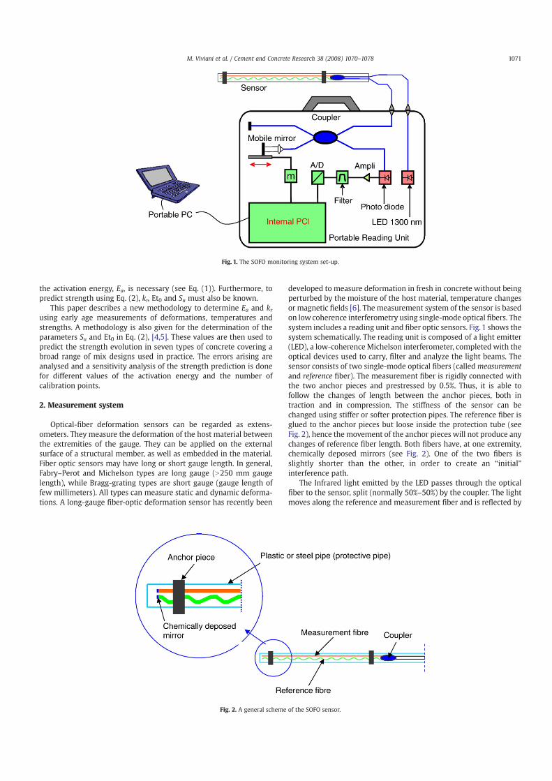
developed to measure deformation in fresh in concrete without beingperturbed by the moisture of the host material, temperature changesor magnetic fields [6]. The measurement system of the sensor is basedon low coherence interferometry using single-mode optical fibers. Thesystem includes a reading unit and fiber optic sensors. Fig. 1 shows thesystem schematically. The reading unit is composed of a light emitter(LED), a low-coherence Michelson interferometer, completed with theoptical devices used to carry, filter and analyze the light beams. Thesensor consists of two single-mode optical fibers (calledmeasurementand reference fiber). The measurement fiber is rigidly connected withthe two anchor pieces and prestressed by 0.5%. Thus, it is able tofollow the changes of length between the anchor pieces, both intraction and in compression. The stiffness of the sensor can bechanged using stiffer or softer protection pipes. The reference fiber isglued to the anchor pieces but loose inside the protection tube (seeFig. 2), hence the movement of the anchor pieces will not produce anychanges of reference fiber length. Both fibers have, at one extremity,chemically deposed mirrors (see Fig. 2). One of the two fibers isslightly shorter than the other, in order to create an “initial”interference path.

The Infrared light emitted by the LED passes through the opticalfiber to the sensor, split (normally 50%–50%) by the coupler. The lightmoves along the reference and measurement fiber and is reflected by

Fig. 1. The SOFO monitoring system set-up.

Fig. 2. A general scheme of the SOFO sensor.

1071M. Viviani et al. / Cement and Concrete Research 38 (2008) 1070–1078

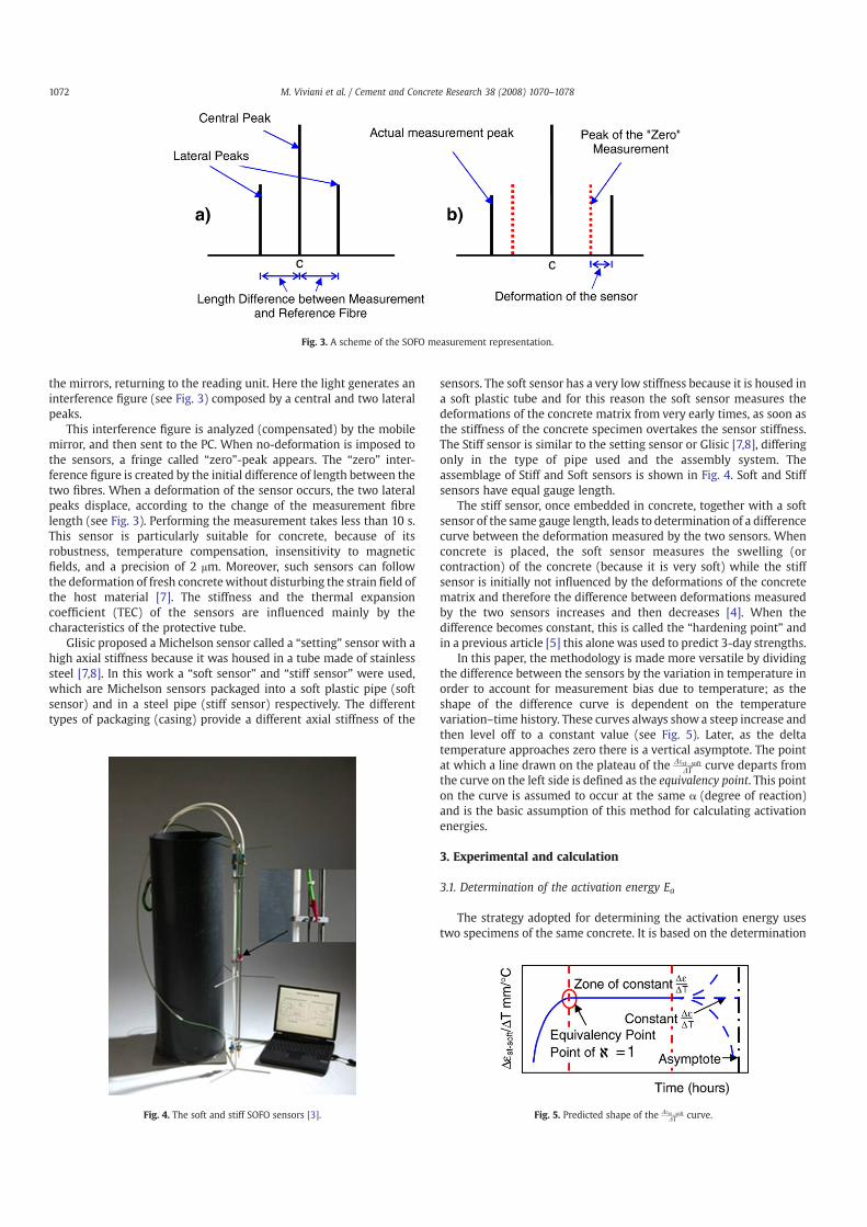
the mirrors, returning to the reading unit. Here the light generates aninterference figure (see Fig. 3) composed by a central and two lateralpeaks.

This interference figure is analyzed (compensated) by the mobilemirror, and then sent to the PC. When no-deformation is imposed tothe sensors, a fringe called “zero”-peak appears. The “zero” inter-ference figure is created by the initial difference of length between thetwo fibres. When a deformation of the sensor occurs, the two lateralpeaks displace, according to the change of the measurement fibrelength (see Fig. 3). Performing the measurement takes less than 10 s.This sensor is particularly suitable for concrete, because of itsrobustness, temperature compensation, insensitivity to magneticfields, and a precision of 2 μm. Moreover, such sensors can followthe deformation of fresh concretewithout disturbing the strain field ofthe host material [7]. The stiffness and the thermal expansioncoefficient (TEC) of the sensors are influenced mainly by thecharacteristics of the protective tube.

Glisic proposed a Michelson sensor called a “setting” sensor with ahigh axial stiffness because it was housed in a tube made of stainlesssteel [7,8]. In this work a “soft sensor” and “stiff sensor” were used,which are Michelson sensors packaged into a soft plastic pipe (softsensor) and in a steel pipe (stiff sensor) respectively. The differenttypes of packaging (casing) provide a different axial stiffness of the

sensors. The soft sensor has a very low stiffness because it is housed ina soft plastic tube and for this reason the soft sensor measures thedeformations of the concrete matrix from very early times, as soon asthe stiffness of the concrete specimen overtakes the sensor stiffness.The Stiff sensor is similar to the setting sensor or Glisic [7,8], differingonly in the type of pipe used and the assembly system. Theassemblage of Stiff and Soft sensors is shown in Fig. 4. Soft and Stiffsensors have equal gauge length.

The stiff sensor, once embedded in concrete, together with a softsensor of the same gauge length, leads to determination of a differencecurve between the deformation measured by the two sensors. Whenconcrete is placed, the soft sensor measures the swelling (orcontraction) of the concrete (because it is very soft) while the stiffsensor is initially not influenced by the deformations of the concretematrix and therefore the difference between deformations measuredby the two sensors increases and then decreases [4]. When thedifference becomes constant, this is called the “hardening point” andin a previous article [5] this alone was used to predict 3-day strengths.

In this paper, the methodology is made more versatile by dividingthe difference between the sensors by the variation in temperature inorder to account for measurement bias due to temperature; as theshape of the difference curve is dependent on the temperaturevariation–time history. These curves always show a steep increase andthen level off to a constant value (see Fig. 5). Later, as the deltatemperature approaches zero there is a vertical asymptote. The pointat which a line drawn on the plateau of the Dest�soft

DT curve departs fromthe curve on the left side is defined as the equivalency point. This pointon the curve is assumed to occur at the same α (degree of reaction)and is the basic assumption of this method for calculating activationenergies.

3. Experimental and calculation

3.1. Determination of the activation energy Ea

The strategy adopted for determining the activation energy usestwo specimens of the same concrete. It is based on the determination

Fig. 3. A scheme of the SOFO measurement representation.

Fig. 4. The soft and stiff SOFO sensors [3]. Fig. 5. Predicted shape of the Dest�softDT curve.

1072 M. Viviani et al. / Cement and Concrete Research 38 (2008) 1070–1078

of the equivalency point of these two specimens. Both specimens havethe same dimensions. They are both monitored with a stiff and a softsensor. Each pair of sensors has the same features. One specimen iswrapped with glass wool. The glass wool acts as insulation and keepsthe temperature of this specimen at a higher level than thetemperature of the other specimen. The rate of reaction in theinsulated cylinder is therefore higher. The temperature is measured inboth specimens (see Fig. 6). The specimens are cured under sealedconditions— nomoisture exchangewith the environment. The degreeof reaction, in terms of equivalent time (Et), can be calculated byEq. (1). For the specimens under sealed conditions the deformation ofthe concrete, εconc, is the sum of the autogenous (εaut) and thermal(εth) deformations:

econc ¼ eaut þ eth ¼ eaut þ TECcTDT ð3ÞThe soft sensor measures the deformation of the concrete matrix fromvery early age because of its low axial stiffness [7,8]. It is assumed thatthe stiff sensormeasures a part of the deformation of concrete that is afunction of the degree of reaction [7]. So the dependence of thedeformation of the stiff sensor on the degree of reaction is expressedby a transfer coefficient ℵ=ℵ(α) which accounts for the percentage ofdeformation that the interface transfers to the sensor. Thus, thedeformation transferred from the concrete to the stiff sensor, εconc→ st

can be expressed as follows:

econcYst ¼ tT econcð Þ ð4ÞHowever, the stiff sensor also changes its length according to thethermal expansion coefficient of the casing (steel in this case), TECsand to the temperature change (see Fig. 7):

esteel ¼ TECsTDT ð5ÞBecause the stiff sensor and the hardening material have different and(in the case of concrete) changing thermal expansion coefficients, thechanging temperature produces additional differences in deforma-tion, termed here thermal interaction deformation εti. This thermalinteraction deformation is proportional to the difference of thermalexpansion coefficients of the two materials (steel and concrete), K.This effect is also influenced by the transfer coefficient. Thus, thisdeformation is measured by the stiff sensor with a magnitudeproportional to the transfer function ℵ=ℵ(α):

etiYst ¼ tT KTDTð Þ ð6ÞTherefore, the total deformation measured by the stiff sensor is thesum of the terms in Eqs. (4)–(6):

est ¼ tT KTDT þ eaut þ TECcTDTð Þ þ TECsTDT ð7ÞThe difference between the deformation measured by the soft and thestiff sensor is determined by Eq. (9):

esoftceconc ¼ eaut þ TECcTDTest ¼ tTKTDT þ tTeaut þ tTTECcTDT þ TECsTDT

�ð8Þ

Dest�soft ¼ t4K4DT þ t� 1ð Þ4eaut þ t� 1ð Þ4TECc4DT þ TECs4DT ð9Þ

In Eq. (9), the term Δεst-soft (t) is the hardening curve [4]. Dividing bothsides of Eq. (9) by ΔT the following equation is obtained:

Dest�soft

DT¼ tTK þ t� 1ð Þ

DTTeend þ t� 1ð ÞTTECc þ TECs ð10Þ

It is assumed that at a certain (critical) degree of reaction (α=α⁎) – theEquivalency Point – the deformation is fully transferred to the stiffsensor (non slip point), i.e. that ℵ(α⁎)=1, in which case Eq. (10)becomes:

Dest�soft

DT¼ K þ TECs ð11Þ

In Eq. (11) the value of Dest�softDT becomes a constant when K becomes

constant. Since the thermal expansion coefficient of steel is constantin time, the coefficient K is constant when the thermal expansioncoefficient of the hardening material is constant. When K is constantEq. (11) describes a horizontal line on a plot of Dest�soft

DT versus time. Afurther analysis of Eq. (11) indicates the possible shapes of theexperimental curves. Two situations might occur:

Dest�softp0DTp0t ¼ 1

Y the curve will level off to a constant value

Dest�soft ¼ 0DT ¼ 0t ¼ 1

Y a vertical asymptote will appear

The two situations are shown in Fig. 5.

The Equivalency Point occurs at a constant degree of reaction for thesame hardening material. This assumption is valid under twonecessary and sufficient conditions. The first is that ℵ=ℵ(α); i.e. theinterfacial bond strength, is a function of the degree of reaction. Thisassumption is supported by the literature which indicates that thecharacteristics of interfaces between bars or fibers and cement-basedmaterials evolve with the degree of reaction [9–11]. The secondassumption is that K (or the TEC of concrete) becomes constant. Fewresults have been found concerning the evolution of thermalexpansion coefficient of concrete in term of degree of reaction [5,12–15]. Howevermany researchers agree to define the TECc as a function ofthe degree of reaction. The Equivalency Point usually appears in thefirst 10–30 h of equivalent time, in the zone where Δε≠0; ΔT≠0.

The definition of Equivalency Point can be used to extract theactivation energy Ea fromhardeningmeasurements. If two specimens ofthe same concrete are monitored with stiff, soft and temperaturesensors but with different temperature regimes (Fig. 8), the equivalencypoint can be determined for each specimen. For both specimens theEquivalency Point occurs at the same equivalent time (maturity).Temperature profiles are inserted in Eq. (1) for each specimen and theintegral is calculated to the Equivalency Point. This results in twoequations with two unknown values (Et and Ea) which can be solved.The values are shown in Table 1.

Fig. 6. Specimens under test.

Fig. 7. Reaction deformation.

1073M. Viviani et al. / Cement and Concrete Research 38 (2008) 1070–1078

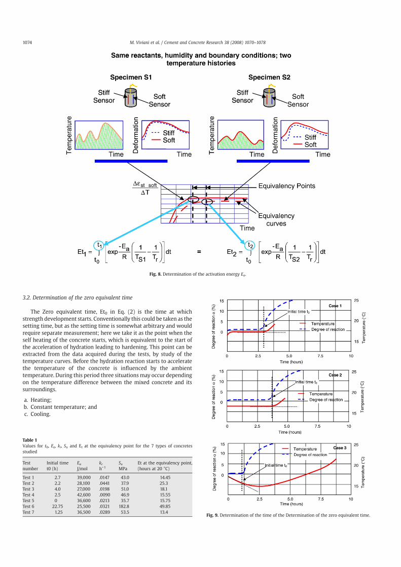
3.2. Determination of the zero equivalent time

The Zero equivalent time, Et0 in Eq. (2) is the time at whichstrength development starts. Conventionally this could be taken as thesetting time, but as the setting time is somewhat arbitrary and wouldrequire separate measurement; here we take it as the point when theself heating of the concrete starts, which is equivalent to the start ofthe acceleration of hydration leading to hardening. This point can beextracted from the data acquired during the tests, by study of thetemperature curves. Before the hydration reaction starts to acceleratethe temperature of the concrete is influenced by the ambienttemperature. During this period three situationsmay occur dependingon the temperature difference between the mixed concrete and itssurroundings.

a. Heating;b. Constant temperature; andc. Cooling.

Fig. 8. Determination of the activation energy Ea.

Table 1Values for t0, Ea, kr, Su and Et at the equivalency point for the 7 types of concretesstudied

Testnumber

Initial timet0 (h)

EaJ/mol

krh−1

SuMPa

Et at the equivalency point,(hours at 20 °C)

Test 1 2.7 39,000 .0147 43.0 14.45Test 2 2.2 28,100 .0441 37.9 25.3Test 3 4.0 27,000 .0198 51.0 18.1Test 4 2.5 42,600 .0090 46.9 15.55Test 5 0 36,600 .0213 35.7 15.75Test 6 22.75 25,500 .0321 182.8 49.85Test 7 1.25 36,500 .0289 53.5 13.4

Fig. 9. Determination of the time of the Determination of the zero equivalent time.

1074 M. Viviani et al. / Cement and Concrete Research 38 (2008) 1070–1078

Situation (a) was never seen in this work, but Et0 can in any case bedetected from the upturn of the temperature curve (case 1, Fig. 9). InSituation (b) Et0 can also be detected when the temperature shows asharp increase (Case 2, Fig. 9). The third situation is the most difficult.Cooling occurs as a consequence of lower external temperature andcan be assumed to be linear in the first hours. The moment when fasthydration begins was therefore taken as the moment when thetemperature curve loses its linearity (see Case 3 in Fig. 9). Thismethodology is directly related to what occurs in each pour ofconcrete and was found to be more relevant than determining thesetting time at a reference temperature and taking this as the Et0 forall the pours of the same concrete. Since the proposed methodologyfor determining Et0 is based on temperature measurements (mon-itored directly in the concrete under testing), there isn't the need offurther separate measurements and the effect of chemicals (such asplasticizers) is taken into account on the rate of reaction. Results forthe 7 concretes studied are reported in Table 1.

3.3. Determination of Su and kr

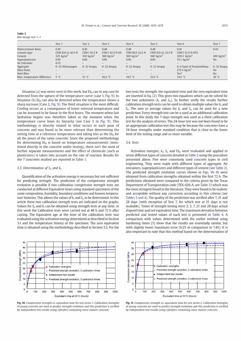
Quantification of the activation energy is necessary but not sufficientfor predicting strength. The prediction of the compressive strengthevolution is possible if two calibration compressive strength tests areconducted at different Equivalent times using standard specimens of thesame composition, humidity, boundary conditions and known tempera-ture histories. This allows the values of kr and Su to be determined. In thisarticle these two calibration strength tests are indicated on the graphs.Values for Su and kr can be obtained using strength tests at any time; inthis work the Calibration tests were carried out at 48 h and 72 h aftercasting. The Equivalent age at the time of the calibration tests wasevaluatedusing theactivation energydetermined as described in Section3.1 and the temperature history of the specimen. The zero equivalenttime is obtained using themethodology described in Section 3.2. For the

two tests the strength, the equivalent time and the zero equivalent timeare inserted in Eq. (2). This gives two equations which can be solved forthe two unknowns (kr and Su). To further verify the results furthercalibration strength tests can be used to obtainmultiple values for kr andSu. The new or average values for kr and Su can be used for a newprediction. Every strength test can be a used as an additional calibrationpoint. In this study the 7-days strength was used as a third calibrationtest for the analysis of errors. The 24-hour test was not been found to bean appropriate calibration test this may be because the concretes have a24-hour strengths under standard condition that is close to the lowerlimit of the testing range and so more variable.

3.4. Tests

Activation energies, kr, Su and Et0 were evaluated and applied toseven different types of concrete detailed in Table 2 using the procedurepresented above. Five were commonly used concrete types in civilengineering. They were made with different types of aggregate. Airentrainers, superplasticizers and different types of cement (see Table 2).The predicted strength evolution curves shown in Figs. 10–16 wereobtained from calibration strengths obtained within the first 72 h. Thepredictions obtained were compared to the criteria given by the TexasDepartment of Transportation code (TEX-426-A, see Table 3) whichwasthemost stringent found in the literature. Theywere found tobe realisticand acceptable without any correction according to this criteria (seeTables 3 and 4). The quality of the predictionwas verified after 7, 21 and28 days (with exception of Test 7, for which test at 21 days is notavailable). Times of strength testing were 2, 3, 7, 21 and 28 days actualelapsed time and not equivalent time. Themaximumdeviation betweenpredicted and tested values of each test is presented in Table 4. Acomparison with values determined with the earlier method usinghardening times [5] show that the results are essentially similar, butwith slightly lower maximum error (6.2% in comparison to 7.4%). It isalso important to note that this method based on the determination of

Table 2Mix-design test 1–7

Test 1 Test 2 Test 3 Test 4 Test 5 Test 6 Test 7

Water/cement Ratio 0.45 0.45 0.48 0.48 0.48 0.18 0.43Cement type CEM II/A-LL 42.5 R CEM I 42.5 R CEM I 42.5 N HS CEM III/A 32.5 N CEM II/A-LL 32.5 R CEM I 52.5 N HTS –

Cement 325 kg/m3 350 kg/m3 360 kg/m3 360 kg/m3 360 kg/m3 1051.1 kg/m3 420 kg/m3

Superplasticizer 0.9% 0.8% 0.8% 0.8% 0.8% 35.1 kg/m3 NoAir Entrainer 0.1% – – – – – –

Aggregate 0–32 Hüttwangen 0–32 Sergey 0–32 Sergey 0–32 Sergey 0–32 Sergey 0–4 Sand of Fontainebleau 0–32 SergeySilica fume – – – – – 273.3 kg/m3 NoSteel fibre – – – – – Yes⁎ NoMax. temperature difference 5 °C 15 °C 20.2 °C 14.5 °C 21.6 °C 14.5 °C 30 °C

Fig. 10. Compressive strength vs. equivalent time for test series 1. Calibration strengthsof young concrete are used to predict strength evolution and this prediction is verifiedby independent test results using cylinders containing more mature concrete.

Fig. 11. Compressive strength vs. equivalent time for test series 2. Calibration strengthsof young concrete are used to predict strength evolution and this prediction is verifiedby independent test results using cylinders containing more mature concrete.

1075M. Viviani et al. / Cement and Concrete Research 38 (2008) 1070–1078

equivalency points is faster and more automated evaluation of theactivation energy than determination of hardening times.

3.5. Estimation of errors

Values for equivalent time are determined using equivalencypoints (see section 3.1). Equivalency points are determined usingmeasurement of temperature and deformation. Errors affectingmeasurement thus affect values for activation energy and subse-quently, strength predictions.

Measurement errors have been estimated for deformation andtemperature using experimental values. Measurement noise whenreading deformation and temperature as well as time dependent driftare especially important when deformation and temperature readingsare added, subtracted multiplied or divided since errors can amplify tobecome high percentages of results that are reported. Propagation oferrors has been estimated in order construct the error envelope forTEC (and for autogenous deformation). The error, Δs, for addition andsubtraction of quantities A and B is calculated as follows:

Ds ¼ffiffiffiffiffiffiffiffiffiffiffiffiffiffiffiffiffiffiffiffiffiffiffiDA2 þ DB2

pð12Þ

Where:

Δs Error related to results of addition or subtraction ofquantities A and B

ΔA Error related to measuring quantity AΔB Error related to measuring quantity B

For multiplication and division of quantities A and B the error iscalculated as follows:

Dr ¼ffiffiffiffiffiffiffiffiffiffiffiffiffiffiffiffiffiffiffiffiffiffiffiffiffiffiffiffiffiffiffiffiffiffiffiDAA

� �2

þ DBB

� �2s

ð13Þ

Δr Error related to results of multiplication or division of thequantities A and B

The equivalency point is assumed to relate to a certain degree ofreaction. This assumption is made on the basis of the mechanism ofdeformation transferring between the hardeningmaterial and sensors.This means that at the equivalency point, the degree of reaction is thesame for all specimens of the same material, hydrating in autogenousconditions. This equivalency is independent of the combination of timeand temperature that has lead to such a degree of reaction.

Determination of Ea requires detection of the equivalency point.Errors in the determination of the equivalency point might result inpoor predictions of activation energy. Drift and noise related tomeasurements introduce an error in terms of time on the equivalencypoint. The worst case scenario for the calculation of the activationenergy corresponds to a bound of ±6 min on values for theequivalency points. This leads to two values for bounds on theactivation energy. The worst case scenario on the value for theactivation energy has been considered. The variation of the activationenergy has an effect on values calculated for strength evolution. The

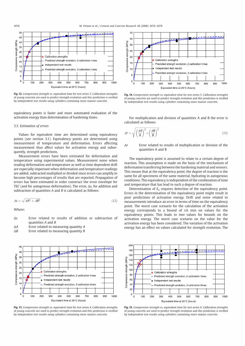
Fig. 12. Compressive strength vs. equivalent time for test series 3. Calibration strengthsof young concrete are used to predict strength evolution and this prediction is verifiedby independent test results using cylinders containing more mature concrete.

Fig. 13. Compressive strength vs. equivalent time for test series 4. Calibration strengthsof young concrete are used to predict strength evolution and this prediction is verifiedby independent test results using cylinders containing more mature concrete.

Fig. 14. Compressive strength vs. equivalent time for test series 5. Calibration strengthsof young concrete are used to predict strength evolution and this prediction is verifiedby independent test results using cylinders containing more mature concrete.

Fig. 15. Compressive strength vs. equivalent time for test series 6. Calibration strengthsof young concrete are used to predict strength evolution and this prediction is verifiedby independent test results using cylinders containing more mature concrete.

1076 M. Viviani et al. / Cement and Concrete Research 38 (2008) 1070–1078

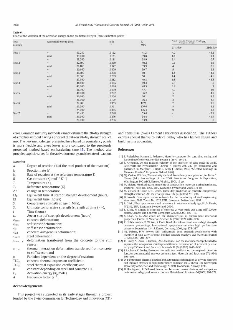
effect of the activation energy variation in strength is shown in Table 5for predictions made using two calibration times and Table 6 forprediction made using three calibrations times (2, 3 and 7 daystrengths). Tables 5 and 6 show that, despite propagation of the errorson measurements, prediction fits in all cases the requirements forprediction of code TEX 426 A (except Test 1, two calibration times,upper bound Ea value). These show the robustness of themethodology.

4. Discussion

The methodology presented here assumes that the EquivalencyPoint is an indicator of the degree of reaction. The good predictionsobtained support this assumption for the range of concretes studied.Constraints on the testing procedure (such as minimum difference intemperature profiles) could be added for a better definition ofhardening time where necessary. The relationship between thehardening curve and the degree of reaction is an important issue forthe extension of the methodology to the general field of hardeningmaterials and this will be the subject of further study. The basis of theproposed methodology allows the thermodynamic-chemical proper-ties (activation energy and rate of reaction) to be determined andconverted to compressive strength via calibration tests. Codifiedmethods use similar concepts by inserting the final setting time intomaturity-strength equations and performing regression analyses.

Currently, maturity methods are still rarely used in practice. Thislack of acceptance is partially related to limited practical experienceand the extensive prior testing needed for calibration of classicalmethods. Confidence in the methodology presented here would beincreased through performing more compressive tests during theearly age of concrete. For example, using a given pair of compressive-strength values, the value of kr and Su are obtained, and a predictivecurve can be calculated. Using other pairs, an envelope of curves isobtained. A standard apparatus for the application of this methodol-

ogy is under development. Since the apparatus is reusable and robust,an inexpensive and in-situ application of the methodology is feasible.

5. Summary and conclusions

Compressive strengths of several widely used concrete mixes havebeen successfully predicted using a procedure that involves early agedeformation monitoring. The procedure has also been applied to aspecial concrete in order to study the applicabilityof themethodology toother types of hardening materials. This methodology allows a fast andaccurate prediction of values for compressive strength on site. Commonmethods for estimation of in place strength requires extensive use ofcuring of mortar cubes at constant temperatures or the use of databasescontaininga large numberof compressive strength valuesmadeatmanyages and cured at different temperatures. These databases have to be fedwith a statistical relevant number of data before a reliable estimation ofthe strength can be made. Furthermore all of these methods requiresmany hours of lab and field time for testing, collecting and analyzingdata. The method here allows strength to be predicted from concretemonitored in situ and early calibration strengths of test specimens fromthe samebatch of concrete— i.e noprior testing is necessary. All thedatacan be obtained from specimens cast at the same time and from thesame batch as the concrete used on site. Seventy-two hours aresufficient to gather data and predict strength evolutionwith less than 7%

Table 4Maximum error between predicted strength and independent test results for themethodology proposed in this paper (equivalency points) and for a previous proposalusing hardening times [4]

Test Maximum errors

Day ofoccurrence ofmax. error

Maximum error %(equivalency points)

Day ofoccurrence ofmax. error

Maximum error %(hardening times)

1 21 +6.2% 7 +4.5%2 28 −6.0% 28 −5.1%3 28 +5.8% 28 +5.1%4 21 −6.1% 21 −7.4%5 28 −5.1% 28 −6.4%6 30 +3.8% 13 +3.7%7 28 +1.3% 8 –

Table 5Effect of the variation of the activation energy on the predicted strength (two calibrationpoints)

Testnumber

Activationenergy J/mol

kr h−1 SuMpa

Predicted strength�Average test strengthAverage test strength 100

7th day 21st day 28th day

Test 1 + 53,250 .0162 41.2 −6.5 −3.5 −10.2mid 39,000 .0147 43.0 −5.4 −1.0 −6.2− 28,200 .0158 41.4 −4.5 0.8 −3.6

Test 2 + 37,400 .0393 38.3 4.1 3.4 5.3mid 28,100 .0441 37.9 4.4 4.1 6.0− 20,600 .0483 40.0 4.6 4.6 6.6

Test 3 + 31,500 .0202 50.7 −1.7 0.3 −5.3mid 27,000 .0198 51.0 −1.9 − .2 −5.8− 23,300 .0195 51.2 −2.0 −0.4 −6.1

Test 4 + 48,800 .0090 47.8 1.3 5.1 1.9mid 42,600 .0090 46.9 1.3 6.1 3.2− 36,900 .0090 46.1 1.3 7.0 4.3

Test 5 + 40,000 .0209 35.9 −1.5 0.9 4.7mid 36,600 .0213 35.7 1.3 1.2 5.1− 26,000 .0204 36.2 0.9 0.5 4.2

Test 6 + 27,900 .0312 183.8 −4.1 −2.3 0mid 25,500 .0321 182.8 −3.8 −1.9 .4− 24,000 .0326 182.1 −3.6 −1.7 .7

Test 7 + 53,450 .0253 55.0 .6 – −2.1mid 36,500 .0289 53.5 1.3 – − .2− 24,000 .0317 52.6 2.1 – 1.2

Fig. 16. Compressive strength vs. equivalent time for test series 7. Calibration strengthsof young concrete are used to predict strength evolution and this prediction is verifiedby independent test results using cylinders containing more mature concrete.

Table 3Verification criteria for maturity prediction; code TEX-426-A. s = predicted strength, s⁎ =independent test results.

Verification criteria Adjusting procedure

s⁎≤0.90 s Develop new S–M relationships⁎≥1.10 s3 consecutiveswithin

Evaluate batching and placement adjust S–M relationship if needed

0.90s≤ s⁎≤0.95s1.05s≤s⁎≤1.10sBetter correlations S–M relationship accepted

1077M. Viviani et al. / Cement and Concrete Research 38 (2008) 1070–1078

error. Common maturity methods cannot estimate the 28-day strengthof amixturewithout havingaprior setof data on28-day strengthof suchmix. The newmethodology, presented here based on equivalencypointsis more flexible and gives lower errors compared to the previouslypresented method based on hardening time [5]. The method alsoprovides explicit values for the activationenergyand the rate of reaction.

Notationα Degree of reaction (% of the total product of the reaction)k Reaction rate h−1

kr Rate of reaction at the reference temperature TrR Gas constant (KJ mol−1 K−1)T Temperature (K)Tr Reference temperature (K)ΔT change in temperature.Et0 Equivalent time at start of strength development (hours)Et Equivalent time (hours)S Compressive strength at age t (MPa),Su Ultimate compressive strength (strength at time t=∞),t Time (hours)t0 Age at start of strength development (hours)εconc concrete deformation;εsoft soft sensor deformation;εst stiff sensor deformation;εaut concrete autogenous deformation;εsteel steel deformation;εconcY st deformation transferred from the concrete to the stiff

sensor;εrY st thermal interaction deformation transferred from concrete

to stiff sensor; andℵ Function dependent on the degree of reaction;TECc concrete thermal expansion coefficient;TECs steel thermal expansion coefficient; andK constant depending on steel and concrete TECEa Activation energy (KJ/mole)A Frequency factor (s−1)

Acknowledgements

This project was supported in its early stages through a projectfunded by the Swiss Commission for Technology and Innovation (CTI)

and Cemsuisse (Swiss Cement Fabricators Association). The authorsexpress special thanks to Patrice Gallay who has helped design andbuild testing apparatus.

References

[1] P. Freiesleben Hansen, J. Pedersen, Maturity computer for controlled curing andhardening of concrete, Nordisk Betong 1 (1977) 19–34.

[2] S. Arrhenius, On the reaction velocity of the inversion of cane sugar by acids,Zeitschrift für Physikalische Chemie 4 (1889) 226–232 [as translated andpublished in Margaret H. Back & Keith J. Laidler, 1967, “Selected Readings inChemical Kinetics” Pergamon, Oxford 1967].

[3] N.J. Carino, H.S. Lew, The maturity method: from theory to application, in: Peter C.Chang (Ed.), Proceedings of the 2001 Structures Congress & Exposition,Washington, D.C. ASCE, Reston, Virginia, 2001, 19 pp.

[4] M. Viviani, Monitoring and modeling of construction materials during hardening,Doctoral Thesis No. 3168, EPFL, Lausanne, Switzerland, 2005, 172 pp.

[5] M. Viviani, B. Glisic, I.F.C. Smith, Three-day prediction of concrete compressivestrength evolution, ACI materials Journal 102 (4) (2005) 231–236.

[6] D. Inaudi, Fiber optic sensor network for the monitoring of civil engineeringstructures, Ph.D. Thesis No. 1612, EPFL, Lausanne, Switzerland, 1997.

[7] B. Glisic, Fibre optic sensors and behaviour in concrete at early age, Ph.D. Thesis,N°2186, EPFL, Lausanne, Switzerland, 2000.

[8] B. Glisic, N. Simon, Monitoring of concrete at very early age using stiff SOFO®sensor, Cement and Concrete Composite 22 (2) (2000) 115–119.

[9] Y. Chan, V. Li, Age effect on the characteristics of fibre/cement interfacialproperties, Journal of Materials Science 32 (19) (1997) 5287–5292.

[10] K. Holshemacher, D. Weisse, S. Klotz, Bond of reinforcement in ultra high strengthconcrete, proceedings, International symposium on ultra high performanceconcrete, September 13–15, Kassel, Germany, 2004, pp. 375–387.

[11] N.J. Delatte, D.W. Fowler, M.S. Williamson, Bond strength development withmaturity of high-early-strength bonded concrete overlays, ACI Materials Journal97 (2) (2000) 201–207.

[12] P. Turcry, A. Loukil, L. Barcelo, J.M. Casabonne, Can the maturity concept be used toseparate the autogenous shrinkage and thermal deformation of a cement paste atearly age? Cement and Concrete Research 32 (9) (2002) 1443–1450.

[13] P. Laplante, C. Boulay, Evolution du coefficient de dilatation thermique du béton enfonction de sa maturité aux tout premiers âges, Materials and Structures 27 (1994)596–605.

[14] Ø. Bjøntegaard, Thermal dilation and autogenous deformation as driving forces toself-induced stresses in high performance concrete, Ph.D. Thesis, The NorwegianUniversity of Science and Technology, N-7491 Trondheim, Norway, 1999.

[15] Ø. Bjøntegaard, E. Sellevold, Interaction between thermal dilation and autogenousdeformation inhighperformance concrete,Materials andStructures34 (2001)266–272.

Table 6Effect of the variation of the activation energy on the predicted strength (three calibration points)

Testnumber

Activation energy J/mol kr h−1

SuMPa

Predicted strength�Average test strengthAverage test strength 100

21st day 28th day

Test 1 + 53,250 .0162 41.2 − .7 −4.3mid 39,000 .0173 39.8 1.8 −1.3− 28,200 .0181 38.9 3.4 0.7

Test 2 + 37,400 .0339 40.2 0.3 1.8mid 28,100 .0377 39.9 .4 2.1− 20,600 .0409 39.7 .5 2.3

Test 3 + 31,500 .0208 50.1 1.2 −4.3mid 27,000 .0209 50 1.4 −4.1− 23,300 .0212 49.8 1.6 −3.8

Test 4 + 48,800 .0086 49.4 2.8 − .7mid 42,600 .0086 48.5 3.9 .7− 36,900 .0090 47.7 4.9 1.9

Test 5 + 40,000 .0202 36.2 .5 4.3mid 36,600 .0204 36.1 .7 4.5− 26,000 .0199 36.3 .3 4.1

Test 6 + 27,900 .0355 177.1 .7 3.1mid 25,500 .0361 176.6 .8 3.3− 24,000 .0365 176.3 .9 3.4

Test 7 + 53,450 .0248 55.4 – −2.8mid 36,500 .0276 54.4 – −1.5− 24,000 .0296 53.9 – .9

1078 M. Viviani et al. / Cement and Concrete Research 38 (2008) 1070–1078