EQUILIBRIA - Jplus Consulting
64
Jplus consulting multivariate analytical technologies User Manual Global Analysis and Reaction Modeling for Chemical Equilibria © Copyright Jplus Consulting Pty Ltd React Lab TM EQUILIBRIA
Transcript of EQUILIBRIA - Jplus Consulting

Jplus consultingmultivariate analytical technologies
User Manual
Global Analysis and Reaction Modeling for Chemical Equilibria
© Copyright Jplus Consulting Pty Ltd
ReactLabTM
EQUILIBRIA

Jplus Consulting Pty Ltd 1 ReactLab™ EQUILIBRIA 1.1
ReactLab™ EQUILIBRIA
Global Analysis and Reaction Modeling for Chemical Equilibria
USER MANUAL
Contents
ReactLab™ EQUILIBRIA ................................................................................................................... 1
ABOUT THIS MANUAL ............................................................................................................ 4
SYSTEM REQUIREMENTS AND INSTALLATION ....................................................................... 4
CONTACT INFORMATION AND SUPPORT .............................................................................. 4
PART 1: REFERENCE GUIDE ........................................................................................................ 5
INTRODUCTION ...................................................................................................................... 5
EXCEL TEMPLATES .................................................................................................................. 5
TITRATION MODES ................................................................................................................. 7
TITRATION DATA, SPECIES AND COMPONENT CONCENTRATIONS ....................................... 8
‘Automatic’ TITRATION MODE ............................................................................................... 9
‘Manual’ TITRATION MODE ................................................................................................. 10
‘pH-Metered’ TITRATIONS ................................................................................................... 10
STARTING THE MATLAB PROGRAM ..................................................................................... 11
Program Operation .............................................................................................................. 12
Load Excel File .............................................................................................................................. 12
Close Excel File ............................................................................................................................. 13
Sync New Data ............................................................................................................................. 13
MODEL ENTRY AND COMPILATION ..................................................................................... 13
Compile Model ............................................................................................................................. 15
PARAMETER ENTRY .............................................................................................................. 16
FITTING THE MODEL TO DATA ............................................................................................. 17
Fit .................................................................................................................................................. 17
Update .......................................................................................................................................... 19
Residuals....................................................................................................................................... 19
Graph GUI ..................................................................................................................................... 21
SIMULATION......................................................................................................................... 22

Jplus Consulting Pty Ltd 2 ReactLab™ EQUILIBRIA 1.1
Simulate........................................................................................................................................ 24
FACTOR ANALYSIS ................................................................................................................ 24
SVD ............................................................................................................................................... 24
EFA ................................................................................................................................................ 25
NUMERICAL OPTIONS .......................................................................................................... 26
Restore Options............................................................................................................................ 26
QUITTING REACTLAB™ ......................................................................................................... 27
Quit ............................................................................................................................................... 27
FIXED SPECTRA ..................................................................................................................... 27
AUXILIARY PARAMETERS ..................................................................................................... 27
NUMERICAL AND OTHER OPTIONS ...................................................................................... 28
HANDLING PROTONATION EQUILIBRIA, [H], [OH] and Kw .................................................. 30
MODEL ENTRY SYNTAX RULES ............................................................................................. 31
PART 2: EXAMPLES ................................................................................................................... 33
Example 1: Simple Equilibrium M+L = ML (M+L.xlsx) ....................................................... 33
The Experiment ............................................................................................................................ 33
The Data ....................................................................................................................................... 33
The Model .................................................................................................................................... 34
Compilation .................................................................................................................................. 35
Total Concentrations of Components .......................................................................................... 36
Definition of Spectra .................................................................................................................... 37
Initial Guesses for the Equilibrium Constant ................................................................................ 37
Update .......................................................................................................................................... 38
Fitting ........................................................................................................................................... 39
Residuals....................................................................................................................................... 40
Measurements at Only One Wavelength ..................................................................................... 41
Example 2: Determination of concentrations of two acids (concAH2.xlsx) ........................ 42
The auxiliary parameters .............................................................................................................. 43
Example 3: Determination of the Protonation Constants of an Indicator (Indicator.xlsx) . 45
Simulation of a measurement ...................................................................................................... 45
The fitting ..................................................................................................................................... 47
Example 4: Ni2+ + ethylenediamine (Ni_en3.xlsx) ................................................................ 49
The model .................................................................................................................................... 49
The data........................................................................................................................................ 50
Fit .................................................................................................................................................. 51
Example 5: Temperature Dependence of logKw .................................................................. 52

Jplus Consulting Pty Ltd 3 ReactLab™ EQUILIBRIA 1.1
Example 6: Two Acids (AH_BH.xlsx) ..................................................................................... 53
Known Spectra ............................................................................................................................. 54
Non-Negative Spectra .................................................................................................................. 55
Example 7: The Complexation of Cu2+ by DANA (3,7-diazanonanedioic acid diamide) (Cu_DANA.xlsx) .................................................................................................................... 55
The experiment ............................................................................................................................ 55
Different definitions of the model ............................................................................................... 56
Example 8: A ‘pH-metered’ titration; Cu2+ with PHE (1,9-Bis(2-hydroxyphenyl)-2,5,8-triazanonane) (Cu_PHE.xlsx) ................................................................................................ 58
The experiment and data entry ................................................................................................... 59
The results .................................................................................................................................... 60
Example 9: The Complexation of Cu2+ by DANA as a ‘pH-metered’ titration (Cu_DANA_pH.xlsx) .............................................................................................................. 61
References ........................................................................................................................... 63

Jplus Consulting Pty Ltd 4 ReactLab™ EQUILIBRIA 1.1
ABOUT THIS MANUAL
This manual is in two parts. Part 1 comprises a comprehensive description of the program architecture and functionality and provides a systematic guide to using it. Part 2 consists of a series of worked examples demonstrating specific analysis case studies using pre-prepared workbooks. All these are provided in the Excel examples folder in the application installation package. Note, when they are installed in the default program files directory they are automatically assigned read-only status but can of course be copied or re-saved to a suitable working directory.
SYSTEM REQUIREMENTS AND INSTALLATION
Please refer to the ‘System Requirements and Installation Guide’ available on our website, and included with the ReactLab™ download.
CONTACT INFORMATION AND SUPPORT
www.jplusconsulting.com
Jplus Consulting Pty Ltd
PO Box 131, Palmyra
WA 6957, Australia
ABN: 83-135-664-603

Jplus Consulting Pty Ltd 5 ReactLab™ EQUILIBRIA 1.1
PART 1: REFERENCE GUIDE
INTRODUCTION
ReactLab™ EQUILIBRIA provides global analysis for fitting the parameters of chemical reaction schemes to multivariate spectroscopic titration data. It also offers extensive reaction modeling and data simulation capabilities.
The program, including all algorithms and the GUI frontend has been developed in Matlab and compiled to produce the final deployable application. It requires the Matlab Component Runtime (MCR) to be installed on the same computer. This allows the program to run on computers without standard Matlab installed. The MCR is supplied as part of the installation package.
All raw data, model entry and results output are organised in Excel Workbooks, which are launched from, and dynamically linked to, the ReactLab™ application. It is therefore necessary for Excel to be installed on the same computer as ReactLab™.
The use of Excel provides a familiar spreadsheet format for all experimental and analysis data and results, and allows the independent application of Excel tools and features for further processing and graphical presentation. It also provides the interface for entering reaction models and all fit related parameters and numerical analysis options. When a workbook is saved it contains all information and settings associated with the current analysis session as well as the numerical data and results. This allows any number of data analyses with different model scenarios and parameter settings to be developed and saved in a self-contained format. These workbooks can be further analysed by ReactLab™ as required or reviewed independently, just using Excel.
The program requires Excel analysis workbooks to retain a strict format, as is provided in the examples and templates.
The process of analysing a data set using the program involves launching ReactLab™ and loading a workbook pre-populated with measurement data. Note, the workbook can be saved or reloaded at any time and will re-synchronise with the ReactLab™ program according to the most recent operation. A selection of example workbooks accompanies the program in an Excel Examples folder and is described in detail in Part 2 of this manual. This guide describes the equilibrium titration implementation of global analysis ReactLab™ EQUILIBRIA. A separate guide describes operation of the complementary kinetic analysis application ReactLab™ KINETICS. Please note that the workbook formats for these applications differ and are therefore not compatible.
EXCEL TEMPLATES
To inspect an Excel ReactLab™ EQUILIBRIA workbook load it directly into Excel or via the ‘Load Excel’ button in the ReactLab™ GUI.
The workbook is pre-formatted containing several worksheets which provide spreadsheet formatted data and results as well as purpose designed model and parameter entry interfaces.

Jplus Consulting Pty Ltd 6 ReactLab™ EQUILIBRIA 1.1
Template Worksheets:
Main The principle model and parameter entry interface
Data Location for experimental or simulated data
Results Location for fitted or simulated concentration profiles and spectra
Residuals Matrix of residuals
Fit Plots Measured and fitted curves as a selection of wavelengths
Sim Simulation parameter entry interface
Aux Used for managing known spectra
SVD Dynamically created sheet for storing SVD or EFA analysis results
About Sheet with contact information and the workbook format version
The format of these sheets is important as ReactLab™ depends on everything being in particular locations. Figure 1 illustrates the organisation and model entry fields in the ‘Main’ worksheet which is the principle sheet of the workbook requiring user interaction. The various fields in this sheet will be described later on in this document.
Figure 1: The ‘Main’ worksheet illustrating a simple metal-ligand titration
Important: The workbooks provided have certain areas of each sheet ‘protected’. These areas include data entry headings (generally highlighted in yellow) and certain key cells containing Excel formulas used to calculate data ranges for ReactLab™ (generally highlighted in grey). It is straightforward to unprotect any sheet using the Excel ‘unprotect’ command, to be found under the ‘Review’ tab. But please be aware that corrupting the layout or formulae will prevent the correct interaction of the spreadsheet with ReactLab™. Exceptions are the red coloured ‘Expand’ tabs on certain worksheets (as in Figure 1). These provide an

Jplus Consulting Pty Ltd 7 ReactLab™ EQUILIBRIA 1.1
increased cell range for complex models if required. To activate these tabs first unprotect the sheet and then expand or contract the cell ranges as required. We suggest re-protecting the sheet afterwards. It is up to the user whether to include a password for re-protection.
To get a practical demonstration of ReactLab™ capabilities quickly refer to the Example workbooks and the corresponding descriptions in Part 2 of this manual. What follows here is a systematic overview of the whole program.
TITRATION MODES
ReactLab™ EQUILIBRIA supports the analysis of titration data gathered by a number of experimental protocols and provides analysis modes to suit. These are illustrated in Figure 2.
Figure 2: Illustration of the different experimental protocols supported by ReactLab for equilibrium investigations
We distinguish two primary titration protocols: ‘Automatic’ or ‘Manual’ each of which can be performed in either ‘Default’ or ‘pH-metered’ configurations and the data analysed accordingly.
The ‘Automatic’ mode is represented in the first column of Figure 2. Equilibrium solutions are prepared automatically by addition of reagent solution from a piston or stepper driven ‘burette’ into a ‘beaker’ and the spectra of a sample of the solution is measured after equilibration. Often this ‘beaker’ is the cuvette in the spectrophotometer. Knowing the experimental volumes, the component concentrations in the ‘burette’ and initially in the ‘beaker’ allows the computation of the total component concentrations in the ‘beaker’ following each addition. These calculations are performed by ReactLab based on this initial information which is entered in the ‘Main’ menu of the workbook.

Jplus Consulting Pty Ltd 8 ReactLab™ EQUILIBRIA 1.1
In ‘Manual’ mode, represented in the second column of Figure 2, individual solutions are prepared independently and their spectra measured. The total component concentrations for each sample have to be entered by the user in the ‘Data’ worksheet of the workbook and ReactLab does not participate in these calculations.
In spectrophotometric titrations, spectra are generally recorded as a function of the total component concentrations in the equilibrated solutions. The solutions are prepared in either ‘Automatic’ or ‘Manual’ mode as described above yielding all participating total component concentrations for each sample. These are then used in subsequent analytical calculations to determine the equilibrium concentrations of all the species in the model. We term this ‘Default’ mode and it is represented in the first row of Figure 2.
In aqueous solutions it is also common (but not required) to measure the pH of each equilibrated solution on-line in automatic titrations, using a pH-electrode, or adjust the pH of each sample to a specific value in manually prepared solutions. In this case the protons are treated differently from the other components involved in the process; the measured pH is used to compute the free proton concentration which is used subsequently for the analysis of the data in conjunction with the other component total concentrations. We call this mode ‘pH-metered’.
To prepare the excel workbook to deal with any of these experimental protocols is straightforward and this is described in the following sections along with a general introduction to titration terminology and analysis.
TITRATION DATA, SPECIES AND COMPONENT CONCENTRATIONS
When working with new measurements start with an empty workbook template. We advise making a copy of ReactLab™_Equilibria_Master_Template.xls/xlsx for this purpose. The first step is to populate the ‘Data’ worksheet with a new measurement matrix Y. This will typically comprise spectra of a titration solution as a function of reagent addition (see Figure 3). The addition volume vector ‘Vadd’ is placed in the column, C7, C8 ..., and the wavelength vector is placed in the row starting at N6, O6 ... The data are placed in an array corresponding to the intersection of the addition and wavelength coordinates. The total number of spectra (n_spectra) and the number of wavelengths (n_lam) are calculated automatically from the data range pasted into the worksheet, see Figure 3.
Important: when using Excel 1997-2003 compatible workbooks the maximum number of wavelengths permitted is 253 (due to the column number restriction in this version of Excel). For Excel 2007 ReactLab™ can in principle handle >17000 wavelengths (the program currently resolves 3 letter column headings = 263 combinations). Note therefore that saving an xlsx workbook in xls format can lead to truncation of large data sets.
Note the columns from D to L are reserved for total volume and total component concentration data. These are either calculated by ReactLab™ in ‘Automatic’ mode or entered by the user in ‘Manual’ mode. In this example ReactLab™ calculates the Vtot vector and the total component concentrations in ‘Automatic’ mode during the fit cycle.

Jplus Consulting Pty Ltd 9 ReactLab™ EQUILIBRIA 1.1
Figure 3: The ‘Data’ sheet, containing the spectra, wavelength range and volumes of added reagent solution.
There is a distinction between components and species in titration experiments. Components are the basic building blocks of the chemical scheme, and whilst they are species in their own right also combine to form other species. For example in the simple metal-ligand scheme:
ML
ML2
K
K
2
M + L ML
ML + L ML
M and L are components as well as species and solutions of these would be made up for the titration experiment. The other species ML and ML2 are formed according to the equilibrium parameters in the scheme. Knowing Mtot, Ltot and the equilibrium constants allows all the individual species concentrations [ML], [ML2] [M] and [L] to be calculated during fitting.
During a typical titration a series of additions are made from a ‘Burette’ to a ‘Beaker’. The data measurement comprises the spectra of the solution in the ‘Beaker’ following each addition. The initial volume Vtot and initial concentrations of the model components in the beaker and burette are provided in the ‘Main’ worksheet. These may be known, or can to be estimated as auxiliary parameters (page 27), during fitting.
Figure 4: Initial concentrations of components and the starting volume (Vtot) are entered in the ‘Main’ sheet after model compilation.
‘Automatic’ TITRATION MODE
In order to calculate the component concentrations in the individual solutions at any point during the titration it is necessary to use this initial information and the Vadd vector to compute the total beaker volume Vtot and total component concentrations [comp]tot. This calculation is done entirely by ReactLab™ in ‘Automatic‘ mode during the update and fitting cycle and the results transferred to the ‘Data’ worksheet for use in subsequent calculations, columns E and F in Figure 3.

Jplus Consulting Pty Ltd 10 ReactLab™ EQUILIBRIA 1.1
‘Manual’ TITRATION MODE
In ‘Manual’ titration mode the automatic calculation of [comp]tot is not performed by ReactLab™. In particular when a series of separate solutions have been made up manually, their equilibrium spectra measured, and the [comp]tot values recorded during preparation. Such data do not necessarily form an automatic series like a conventional titration and can be completely arbitrary mixtures of the reaction components. These can still be fitted to an equilibrium model using ReactLab™ EQUILIBRIA.
The data are placed in the spreadsheet as normal, but the Vadd vector should now be replaced with a simple index vector 1....n to act as a default x-axis for ReactLab™ and other plots.
Once the required reaction model has been compiled, the known [comp]tot values should be entered under the appropriate component headings in the ‘Data’ sheet.
To select ‘Manual’ analysis mode it is necessary to disable the ‘Automatic’ mode re-calculation of these [comp]tot values by ReactLab™. To do this, leave the Vtot field in the ‘Main’ sheet blank. When ReactLab™ identifies a blank in this field it will use the supplied [comp]tot data for the speciation calculations. Note: all the other ‘Beaker’ and ‘Burette’ fields as well as the Vtot column in the ‘Data’ sheet are also ignored.
Once the data is in place the workbook it should be saved under a suitable name. It must be saved first and re-loaded into the ReactLab™ program even if previously opened by it, in order for the new data to be recognised by ReactLab™.
‘pH-Metered’ TITRATIONS
In pH-metered titrations the pH of each solution is measured using a pH electrode, or in manual mode each sample has had its pH adjusted to a known value. ReactLab EQUILIBRIA will switch to pH-metered analysis mode automatically, depending on whether the measured pH vector is provided in the ‘Data’ worksheet.
In order to declare a titration as ‘pH-metered’ the column M of the ‘Data’ worksheet must contain the entry ‘pH’ in cell M6. The cells below should be populated with the pH values of the different solutions (see Figure 5). The entry ‘pH’ is used by ReactLab to decide whether titration data is to be analysed using the ‘Default’ computations or utilise the measured pH.
Figure 5: The ‘Data’ Sheet from Example 8 showing the inserted measure pH vector in column M with the heading ‘pH’ in cell M

Jplus Consulting Pty Ltd 11 ReactLab™ EQUILIBRIA 1.1
In a ‘pH-metered’ titration analysis all the total component concentrations, with the exception of [H]tot are calculated automatically from the initial component concentrations and beaker and burette volumes in the ‘Main’ worksheet. The [H]tot vector (from which the [H]free would otherwise be determined) is now redundant and ignored. All speciation calculations instead use the [H]free values derived from the pH vector in the ‘Data’ sheet. Indeed there is no need to provide initial concentrations for [H] in the beaker and burette as these parameters are redundant in this calculation mode. The subsequent calculations will lead to a meaningless [H]tot vector in the data sheet of course but this can be ignored.
Advanced note: The [H]tot column has been left in place since it is possible to compare a volumetric calculation of [H]tot with the apparent total determined by the measured pH. This is demonstrated in Example 9.
For a ‘Manual pH-metered’ titration the pH measurements are provided in the ‘Data’ sheet as above. Follow the earlier procedure to enforce ‘Manual’ mode titration analysis and leave the Vtot cell in the ‘Main’ data sheet blank along with the other initial concentrations. Enter the total component concentrations of the equilibrium mixtures in the columns of the ‘Data’ sheet (as for a default manual titration) but leave the [H]tot vector blank. The pH entries in column M will be used in all speciation calculations.
STARTING THE MATLAB PROGRAM
When ReactLab™ is launched it also requires the Matlab MCR to initialise. This can take a while and is very much dependant on computer performance, after which the ReactLab™ GUI appears as in Figure 6.
Figure 6: Matlab GUI control panel at startup
This GUI provides the main control interface for the program with a series of pushbuttons on the right hand side for key functions. These provide all the ReactLab™ program commands and their operation is described over the following pages.
Note depending on the workbook status (e.g. whether a data or model are present) some of these functions may be disabled.

Jplus Consulting Pty Ltd 12 ReactLab™ EQUILIBRIA 1.1
In addition an About menu item at the top left provide details of the ReactLab™ version and licensing information.
Program Operation
Load Excel File
Press ‘Load Excel File’ in the ReactLab™ GUI to select and link to an Excel Workbook. This will launch a new instance of Excel and load the requested workbook independent of any other open Excel workbooks. Only Equilibrium workbook templates can be loaded into this version of ReactLab™.
Important: Excel is launched as an ActiveX server in an independent process linked to ReactLab™ which communicates with it through its Microsoft component object model (COM) interface. The launch of Excel and ActiveX server linkage is initiated by the Matlab program. Linking to an already open workbook in Excel is NOT supported. If a workbook is prepared for analysis following the steps above it should first be saved and re-opened from the running ReactLab™ application. Note all Excel functionality is available to manipulate the workbook as normal while it is linked to ReactLab™.
We will use a simulation of a reaction scheme M+L=ML and M+2L=ML2 in the following sections to illustrate ReactLab™ features. The workbook M+2L.xlsx contains this example and the simulated data has been in turn used to illustrate the fitting process by “optimising” the parameters of the model used to create it.
When a workbook is first loaded various displays of data or fitted results are created in the Matlab GUI depending on its contents. On loading this example workbook M+2L.xls the graphics are fully restored reflecting the results of fitting the simulated data to the reaction model (Figure 7).
Figure 7: The ReactLab™ GUI display reflects the Workbook content when it is loaded. This shows the data residuals, fitted concentration profiles and spectra of all absorbing species for the Excel M+2L.xlsx workbook.

Jplus Consulting Pty Ltd 13 ReactLab™ EQUILIBRIA 1.1
Note the toolbar, top left, offers zooming and rotating tools for the plots. These are inbuilt Matlab features. Right clicking on a graph while in any of these modes provides a number of supplementary options or constraints.
When data are present in the workbook they are also displayed in a separate Matlab figure window:
Figure 8: 3D Data display (M+2L.xlsx)
Close Excel File
This will, on confirmation, close the current workbook and link, prior to opening another. If any changes have been made to the workbook the user must first switch focus to the workbook where he/she will be prompted as to whether the changes to the workbook need to be saved.
Sync New Data
Press this to synchronise new or edited data in a workbook with ReactLab™ without having to save and re-load it (this was required prior to version 1.1 Build 03). The new or modified data will be displayed in the ReactLab figure window.
MODEL ENTRY AND COMPILATION
Before analysing data or computing a simulation it is necessary to enter a reaction model and compile it. All model information is placed in the Excel Workbook in the ‘Main’ worksheet. The scheme corresponding to the example we are using can be represented as in Figure 9. Note each reaction step is entered individually M+L=ML and M+2L=ML2 which allows for a one-to-one correspondence of each reaction step to its parameter value in the ‘Parameter’ column (parameters values and labels are not required for the compilation step).

Jplus Consulting Pty Ltd 14 ReactLab™ EQUILIBRIA 1.1
Figure 9: The 2 step equilibrium expressed using the formation constant format
Note for equilibrium fitting the model can be expressed either in terms of formation constants (β’s) as above or in the alternative perhaps more intuitive format of association constants (K’s). Using the latter format and the same equilibrium constants, the model would appear as in Figure 10.
Figure 10: The 2 step equilibrium expressed using the association constant format
The two approaches yield distinct parameters, though these can be inter-converted quite easily. In this example:
logβ11 = logK1
logβ12 = logK1 + logK2
This relationship can be extrapolated for higher coordinations:
logβ1n = logK1 + logK2 ...+ logKn
One of the merits of the β format is that all complexes can be unambiguously assigned a formation constant with a unique numerical subscript even when further components are involved. This is less straightforward with association constants.
In both cases parameter values are always expressed as a log value which can be positive or negative or indeed zero. This simply means the true parameter value (i.e. anti-logged) is less than or greater than 1 which is permissible for both types of constant.
A discussion of these alternative representations can be found in Marcel Maeder, Yorck-Michael Neuhold. Practical Data Analysis in Chemistry, Elsevier 2007, and in the explanations to Example 7.
The key point is that either format will be interpreted correctly by ReactLab™.
Note integers preceding a species letter or string are interpreted as stoichiometry coefficients for the species in question e.g. M+2L = ML2. A trailing integer is used to represent higher coordination complexes e.g. ML, ML2, ML3 etc. Essentially, ‘normal’ chemical reaction equations can be written. For further information on the syntax rules see page 31.
In all cases a label for each parameter can be provided. This allows easier reference to mechanisms with multiple steps. These labels and the parameter values themselves are not required prior to compilation (see Parameter Entry below).

Jplus Consulting Pty Ltd 15 ReactLab™ EQUILIBRIA 1.1
Important: It is necessary for any new entry in the Excel workbook to be properly completed i.e. by hitting return or pressing the arrow key to take the focus away from the cell in question once the desired value has been assigned, otherwise the ‘Incomplete worksheet entry’ warning will be raised. Failing to enter values properly prevents ReactLab™ from accessing the worksheet cell through the ActiveX interface.
Compile Model
When model entry is complete press the ‘Compile Model’ button.
ReactLab™ reads in the model and translates it into an internal coefficient form. It identifies all the participating species in the model and extracts all the starting components from which all the other species are formed through the model equilibrium relationships. These are listed in fields in the ‘Main’ worksheet. Initial total component concentrations are entered for the ‘Beaker’ and ‘Burette’ (if this is a conventional titration – see ’Automatic’ TITRATION MODE on page 9)
Figure 11: Fields for entering the initial component concentrations and the initial volume in the ‘Beaker’ Vtot.
Certain key values are calculated automatically by Excel and are required by ReactLab™, namely the number of reactions specified in the model for which there is an equilibrium constant field (n_par), the number of individual chemical species in the mechanism (n_species) and the number of auxiliary parameters (n_aux_par). Do not overwrite the formulae in these cells (they are protected in the templates supplied).
Figure 12: Model information automatically generated in Excel
Note it is not necessary to enter any other species concentrations. These are calculated from the total component concentrations of each equilibrium mixture following titrant addition from ‘Burette’ to ‘Beaker’.
Species headings are also written to the Sim, ‘Results’ and ‘Aux’ worksheets for subsequent data output. Any previous results are cleared at this point.
Auxiliary parameters are an advanced feature which can be ignored during program familiarisation, though this feature can be used for fitting other parameters, e.g. unknown component concentrations (See Auxiliary Parameters on page 27).

Jplus Consulting Pty Ltd 16 ReactLab™ EQUILIBRIA 1.1
PARAMETER ENTRY
Prior to fitting (or simulation), numerical parameter estimates or known values if they are available from other work should be entered in the appropriate fields of the ‘Main’ sheet (Figure 13). The log of the Equilibrium or Formation constants must be entered e.g. 3 for K=103M-1.
The user must decide whether parameters will be either fixed (, kept constant) or fitted (, optimised) using the tick boxes.
Figure 13: Labeling and entering parameters and selecting those to ‘fit’.
The spectral status of each species must be assigned ‘colored’, ‘non-abs’ or ‘known’ using the corresponding drop down box.
Figure 14: Setting the spectral status of each species
Defining a species as ‘coloured’ means it is predicted to have a spectrum contributing to the measurement, i.e. it absorbs in the wavelength range covered by the measurement. ‘Colored’ spectra will be calculated and optimised during the analysis. A ‘non-abs’ species will be fixed as colourless, meaning the species is invisible in the measurement. Selecting ‘known’ allows an existing spectrum to be supplied for a species. For example this may be for a reagent or product whose spectrum can be measured independently or for a species whose spectrum is known from other work. It must be pasted under the corresponding species name in the ‘Aux’ sheet prior to an ‘Update’ or ‘Fit’ otherwise an error will be raised. It is essential it is in a compatible format to the experimental or simulated data with the same number of wavelengths and in correct Molar extinction units (for further information, see FIXED SPECTRA on page 27).
Jplus Consulting Pty Ltd 17 ReactLab™ EQUILIBRIA 1.1
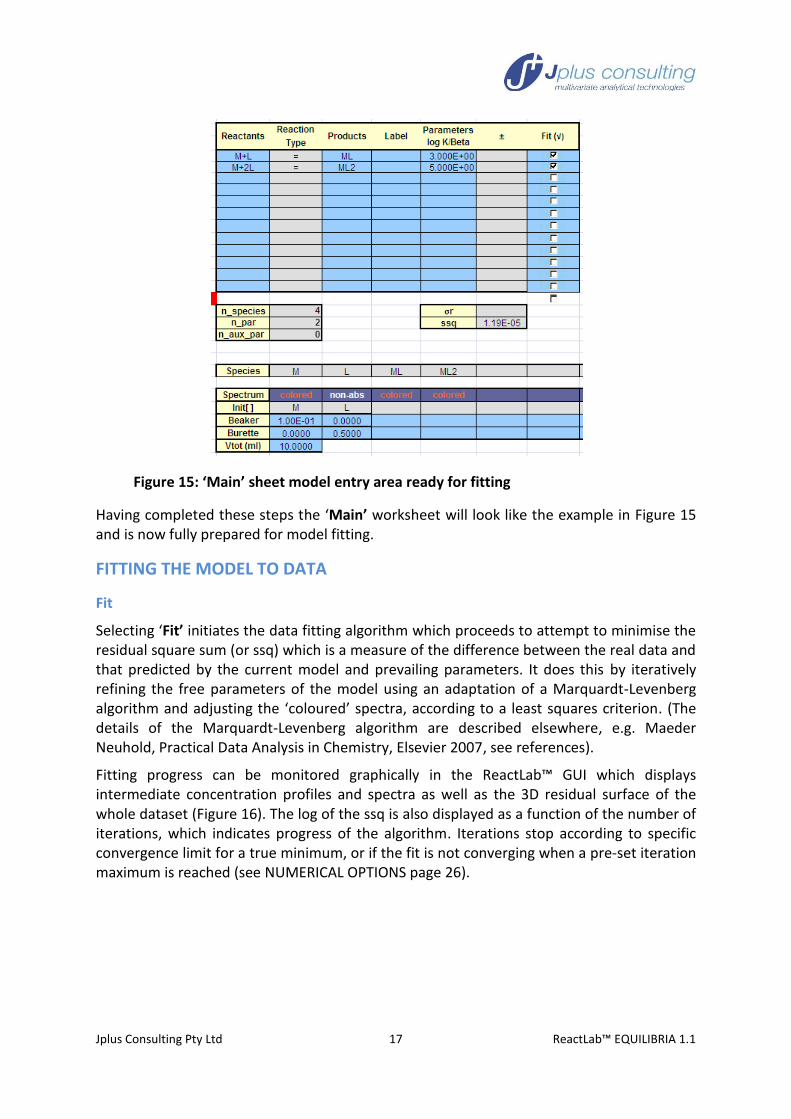
Figure 15: ‘Main’ sheet model entry area ready for fitting
Having completed these steps the ‘Main’ worksheet will look like the example in Figure 15 and is now fully prepared for model fitting.
FITTING THE MODEL TO DATA
Fit
Selecting ‘Fit’ initiates the data fitting algorithm which proceeds to attempt to minimise the residual square sum (or ssq) which is a measure of the difference between the real data and that predicted by the current model and prevailing parameters. It does this by iteratively refining the free parameters of the model using an adaptation of a Marquardt-Levenberg algorithm and adjusting the ‘coloured’ spectra, according to a least squares criterion. (The details of the Marquardt-Levenberg algorithm are described elsewhere, e.g. Maeder Neuhold, Practical Data Analysis in Chemistry, Elsevier 2007, see references).
Fitting progress can be monitored graphically in the ReactLab™ GUI which displays intermediate concentration profiles and spectra as well as the 3D residual surface of the whole dataset (Figure 16). The log of the ssq is also displayed as a function of the number of iterations, which indicates progress of the algorithm. Iterations stop according to specific convergence limit for a true minimum, or if the fit is not converging when a pre-set iteration maximum is reached (see NUMERICAL OPTIONS page 26).

Jplus Consulting Pty Ltd 18 ReactLab™ EQUILIBRIA 1.1
Figure 16: Jplus GUI following fit convergence: Note random residual surface
Statistical output includes standard deviations for each fitted parameter (including auxiliary parameters), as well as the sum-of-squares, ssq, and the standard deviation for the residuals, σr (Figure 17).
Figure 17: ‘Main’ worksheet following fit convergence: Note optimized parameters and errors and the final ssq.
During iterations the intermediate and final best fit results are also updated numerically in the ‘Main’ Excel worksheet and the concentration and spectra matrices in the ‘Results’ worksheet. Any Excel graphs linked to these data ranges will be updated accordingly (Figure 18). The implementation of such graphs is entirely at the discretion of the user, and these can of course be created and manipulated entirely independently of ReactLab™.
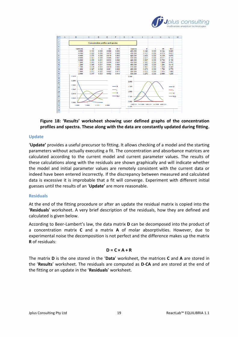
Jplus Consulting Pty Ltd 19 ReactLab™ EQUILIBRIA 1.1
Figure 18: ‘Results’ worksheet showing user defined graphs of the concentration profiles and spectra. These along with the data are constantly updated during fitting.
Update
‘Update’ provides a useful precursor to fitting. It allows checking of a model and the starting parameters without actually executing a fit. The concentration and absorbance matrices are calculated according to the current model and current parameter values. The results of these calculations along with the residuals are shown graphically and will indicate whether the model and initial parameter values are remotely consistent with the current data or indeed have been entered incorrectly. If the discrepancy between measured and calculated data is excessive it is improbable that a fit will converge. Experiment with different initial guesses until the results of an ‘Update’ are more reasonable.
Residuals
At the end of the fitting procedure or after an update the residual matrix is copied into the ‘Residuals’ worksheet. A very brief description of the residuals, how they are defined and calculated is given below.
According to Beer-Lambert’s law, the data matrix D can be decomposed into the product of a concentration matrix C and a matrix A of molar absorptivities. However, due to experimental noise the decomposition is not perfect and the difference makes up the matrix R of residuals:
D = C × A + R
The matrix D is the one stored in the ‘Data’ worksheet, the matrices C and A are stored in the ‘Results’ worksheet. The residuals are computed as D-CA and are stored at the end of the fitting or an update in the ‘Residuals’ worksheet.

Jplus Consulting Pty Ltd 20 ReactLab™ EQUILIBRIA 1.1
Figure 19: The residuals as a 3-D plot in the excel format
The residuals can be represented in a 3-D plot as demonstrated in Figure 19 in the excel format. They are also part of the Jplus GUI as shown in Figure 16.
The main purpose is to enable the construction of plots that demonstrate the quality of the analysis in a readily publishable format. Naturally, the user can also apply any additional statistical analysis to the residual matrix.
The worksheet ‘Fit Plots’has been created for the preparation of plots that compare the measured data points to the fitted curves at a total of five wavelengths. The experienced excel user will be able to expand the number of curves/wavelengths with little effort.
Figure 20: Plot of the measured data (different markers) and fitted curves (lines) in the ‘Fit Plots’ worksheet
Figure 20 shows the default format in the ‘Fit Plots’ worksheet. Markers, line styles and colours can be adapted by the user to any preferred format in the usual excel way.
400
440
480520
560600
-4.E-04
-3.E-04
-2.E-04
-1.E-04
0.E+00
1.E-04
2.E-04
3.E-04
4.E-04
resi
du
als
time
-0.0200
0.0000
0.0200
0.0400
0.0600
0.0800
0.1000
0.1200
0.1400
0 1 2 3 4 5 6
Y_meas 400
Y_meas 450
Y_meas 500
Y_meas 550
Y_meas 600
Y_calc 400
Y_calc 450
Y_calc 500
Y_calc 550
Y_calc 600

Jplus Consulting Pty Ltd 21 ReactLab™ EQUILIBRIA 1.1
Figure 21: Section of the ‘Fit Plots’ worksheet, the user can select the wavelengths in the blue cells D2:H2
The worksheet is populated by a selection of five wavelengths covering the complete wavelength range in the blue cells D2:H2. The user can change the wavelengths to any other values, the rest is done automatically by excel. Invalid wavelengths results in removal of the trace, thus if the measurements at only one wavelength should be displayed, the remaining four entries are set to an invalid number, i.e. outside the measured range.
Please note the ‘Fit Plots’ worksheet is provided by the authors to demonstrate the use of Excel functionality to process and chart data from elsewhere in the workbook, in this specific case for presenting residual plots. It is not necessary for ReactLab analysis functionality and can be deleted from all workbooks if it is not required.
Graph GUI
This will launch a standalone GUI figure which allows close inspection of individual fitted spectra and concentration profiles either together or individually. The real data can be superimposed on the best fit curves along with separate residual plots. A slider control is available for easily scanning through the individual traces. Modes for autoscaling are available as well as the ability to plot the y-axis logarithmically which can be useful for visualising intermediates occurring at very low concentrations. The best fit concentration profiles and intermediate spectra can also be displayed here. Again a toolbar provides access to plot zooming.

Jplus Consulting Pty Ltd 22 ReactLab™ EQUILIBRIA 1.1
Figure 22: Example displays in the Graph GUI window
Right clicking within the display area will open a context sensitive menu allowing the current graph to be pasted to the Windows clipboard for direct transfer to other applications such as Microsoft Word.
It is also possible to print any plot from this display and a print preview facility is provided to align and size the output graph.
Figure 23: Print preview launched from the Graph GUI window
SIMULATION
Simulation enables the creation of artificial data sets for model evaluation and comparison with real scenarios. It is an extremely useful adjunct to the fitting functionality and very informative when used as a ‘what if’ tool. It also allows an easy route to familiarisation with the ReactLab™ application.
The first step in simulation involves provision and compilation of a model as described earlier on (page 13 onwards), and providing parameter values for the reaction equilibria. However instead of calculating the concentration profiles as a precursor to fitting the model

Jplus Consulting Pty Ltd 23 ReactLab™ EQUILIBRIA 1.1
to experimental data, these are instead combined with artificial spectra to synthesise a new simulated data set.
Gaussian curves are used for the artificial spectra. The parameters defining these are provided along with a titration addition sequence and the wavelength range required for the simulated data in the ‘Sim’ Excel worksheet shown in Figure 24.
Figure 24: the ‘Sim’ worksheet showing data simulation parameters
It is necessary to provide three parameters for each Gaussian spectrum - the position of the maximum on the wavelength axis, the Gaussian peak half-width (in wavelength units) and its height (equivalent to the maximum extinction coefficient for an absorbance spectrum). The calculated Gaussian curves will be used as molar absorption spectra for the appropriate species in the simulation. Simply leave the Gaussian parameters blank if it is intended that a species be modelled as colourless (or set its height to zero). The overall wavelength and titration addition ranges and their resolution are entered in corresponding ‘start’, ‘step’ and ‘end’ fields. The resulting absorption spectra are shown in Figure 25. The noise parameter will add an overall percentage of Gaussian noise relative to the maximum overall absorbance of the simulated data set.
Figure 25: The absorption spectra created by the parameters of Figure 24
-0.500
0.000
0.500
1.000
1.500
2.000
2.500
400.000 450.000 500.000 550.000 600.000
M
ML
ML2

Jplus Consulting Pty Ltd 24 ReactLab™ EQUILIBRIA 1.1
Note: When a simulation is calculated all pre-existing data and results in the worksheet will be overwritten or removed.
The model species list is automatically copied to the ‘Sim’ worksheet at compilation time. Initial concentrations of the components for this simulation must be entered in the ‘Main’ sheet in the usual place. Note however the spectra status settings in the ‘Main’ sheet (‘colored’/’known’ etc.) are ignored in the simulation calculation.
Simulate
Selecting ‘Simulate’ will create a synthetic dataset and populate the ‘Data’ and ‘Results’ worksheets with the results of the simulation.
Data created by simulation can subsequently be analysed in the same way as experimental data using the fitting procedures already described above. This allows different model scenarios to be tested as candidate mechanisms in particular providing a means of testing for the ‘resolvability’ of the data/model combinations.
Simulation also provides an invaluable general educational tool for learning and understanding the behaviour of linked equilibrium processes. For example it provides an easy route to investigating the importance and use of ‘known spectra’ in the determination of complex models, since the Gaussian spectra used in the simulation and which now appear in the ‘Results’ sheet can be simply cut and paste to the ‘Aux’ sheet for experimentation.
Simulation does not produce ‘pH-metered’ titrations. If required, simulate default volume-titrations and extract pH to put into pH column
FACTOR ANALYSIS
Factor analysis is provided as an additional tool that can be used to estimate the number of coloured components in any data set thereby providing insight into process complexity. The two principle algorithms used are singular value decomposition (SVD) and in conjunction with the results of this, evolving factor analysis (EFA). The critical difference between this and the ReactLab™ model fitting functionality is that these analyses are model free and do not yield reaction mechanism or equilibrium constant information.
SVD is an incredibly useful algorithm, mathematically decomposing a matrix Y into three matrices such that Y=U·S·V. Put very simply, these matrices comprise the eigenvectors and eigenvalues of the original data matrix. These define the data in terms of the linearly independent components along with their significance. This correlates with the underlying chemical complexity, by (a) defining the minimum number of species required in a reaction model and (b) the maximum no of independent coloured species in the model. The user is referred to the references on page 55 for further information.
SVD
This opens a new GUI window which graphically displays a reduced subset of the singular value decomposition of the data matrix.

Jplus Consulting Pty Ltd 25 ReactLab™ EQUILIBRIA 1.1
Figure 26: The SVD GUI
The graphs display the selected number of concentration and spectral basis vectors of the decomposition (essentially the eigenvectors of Y which reside in the columns of U and rows of V) and lists the corresponding singular values (from the diagonal matrix S). The number of significant singular values (equivalent to the number of principle eigenvectors, n_ev) over the noise background is equal to the number of linearly independent coloured components in the system. The corresponding eigenvectors, whilst not representing real spectra or concentration profiles represent the set of linearly independent vectors from which all the data can be re-composed by linear re-combination. The number selected here is used to determine a reduced decomposition to save in the Excel worksheet. (Saving of SVD and complimentary EFA results is done from the EFA GUI below).
EFA
This opens a GUI window providing basic model free evolving factor analysis of the current data.
Evolving Factor Analysis provides a model free approach to predicting concentration profiles and spectra of coloured components in the data. It results in some indication of spectral shapes and the evolution of independent species during the measurement, which can offer useful insight into appropriate reaction models for fitting (for example compare the concentration profiles and spectra in Figure 27 with the fitted equivalents in Figure 18). Note that the concentration profile of non-absorbing L does of course not appear in the EFA result. Thus, EFA cannot account for all four species in the simulation and required for the model based ReactLab™ analysis; EFA only ‘sees’ the colored species. This is one of the drawbacks of model free approaches as compared to hard modeling to fundamental reaction mechanisms.
Jplus Consulting Pty Ltd 26 ReactLab™ EQUILIBRIA 1.1
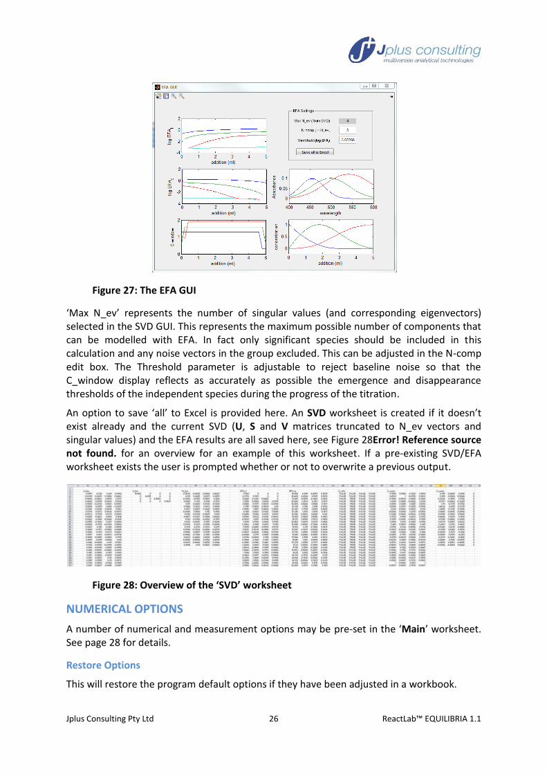
Figure 27: The EFA GUI
‘Max N_ev’ represents the number of singular values (and corresponding eigenvectors) selected in the SVD GUI. This represents the maximum possible number of components that can be modelled with EFA. In fact only significant species should be included in this calculation and any noise vectors in the group excluded. This can be adjusted in the N-comp edit box. The Threshold parameter is adjustable to reject baseline noise so that the C_window display reflects as accurately as possible the emergence and disappearance thresholds of the independent species during the progress of the titration.
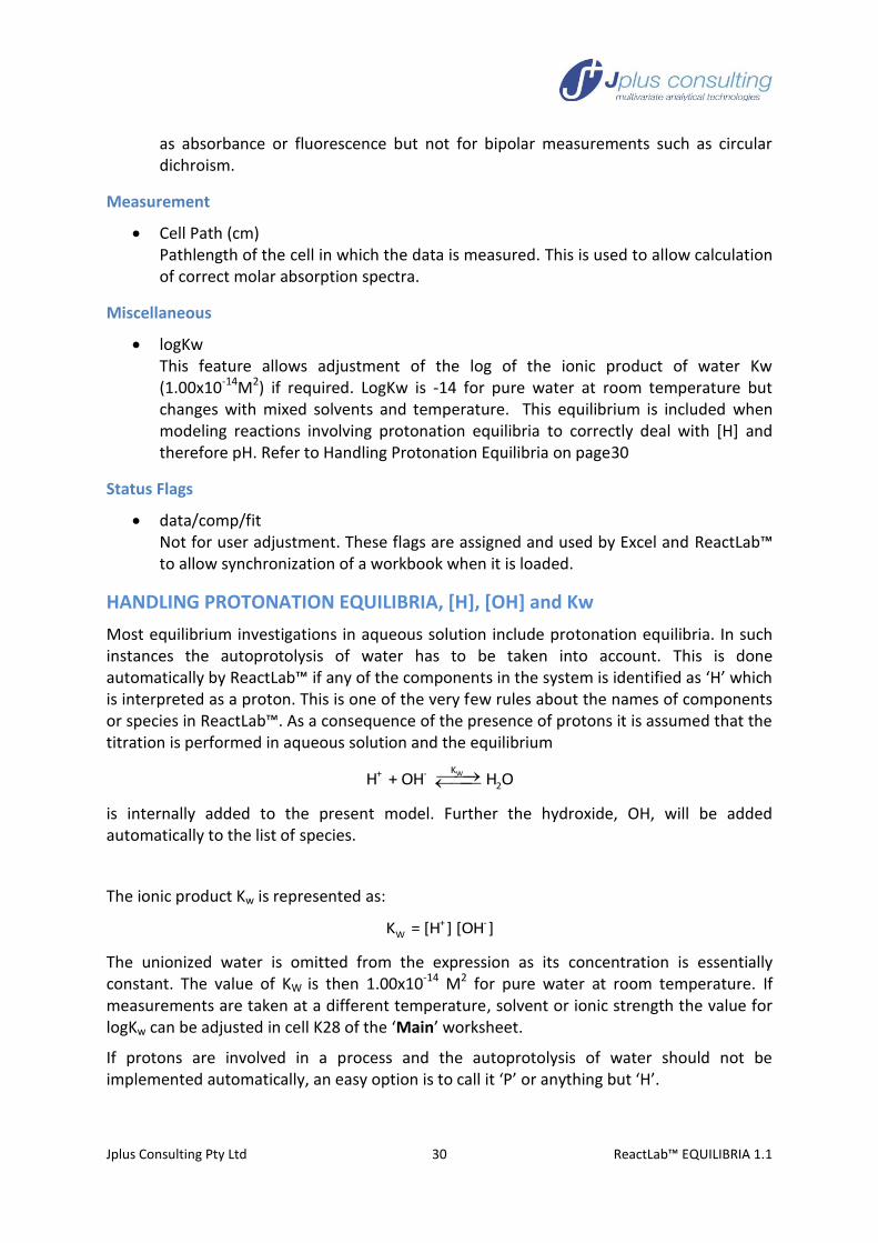
An option to save ‘all’ to Excel is provided here. An SVD worksheet is created if it doesn’t exist already and the current SVD (U, S and V matrices truncated to N_ev vectors and singular values) and the EFA results are all saved here, see Figure 28Error! Reference source not found. for an overview for an example of this worksheet. If a pre-existing SVD/EFA worksheet exists the user is prompted whether or not to overwrite a previous output.
Figure 28: Overview of the ‘SVD’ worksheet
NUMERICAL OPTIONS
A number of numerical and measurement options may be pre-set in the ‘Main’ worksheet. See page 28 for details.
Restore Options
This will restore the program default options if they have been adjusted in a workbook.

Jplus Consulting Pty Ltd 27 ReactLab™ EQUILIBRIA 1.1
QUITTING REACTLAB™
Quit
This will ask for confirmation before both closing the Excel workbook and then ReactLab™.
FIXED SPECTRA
In addition to the option to define species as colourless, the known spectrum feature allows predetermined spectra to be assigned to species prior to model fitting. During the fitting the fixed spectra are not adjusted. The benefits of using fixed spectra are significant and discussed in the context of worked examples in Part 2.
When a model is compiled, a corresponding species list is created in the ‘Aux’ worksheet. Known spectra should be cut and pasted under the appropriate species name. That species should be selected as ‘known’ in the ‘Main’ worksheet.
Note: Fixed spectra must be provided in units of Molar Absorptivity (i.e. the fictional absorption spectrum of a 1M solution measured in a 1cm pathlength cuvette).
The easiest way to experiment with this feature is to simulate data to a particular model and copy and paste the simulated spectra from the ‘Result’ sheet to the ‘Aux’ sheet species columns. These then correspond to the spectra from which the simulated data set was calculated and can be selected as ‘known’ for species during experimental fitting.
AUXILIARY PARAMETERS
The auxiliary parameter feature is unique to ReactLab™ and depends on the parallel execution available through the independent Excel process.
Auxiliary parameters are treated like ‘normal’ parameters during fitting but can be used to define arbitrary relationships between virtually any of the workbook data or conventional parameters involved in the fitting calculations.
The feature works using Excel formulas and depends on the fact that at key points of each fit iteration parameters are written out and read back from excel but not before the execution of the any excel cell formula defining relationships between them.
Thus an auxiliary parameter can be set up to determine the concentration of an unknown component in a titration experiment (see Figure 29). This can be achieved by linking the component starting concentration value to an auxiliary parameter. In this example we wish to determine [M]0 in the beaker. This is normally entered in as a static value in cell C37 when it is known. Instead a formula (=K7) is placed in C37 linking its value to the auxiliary parameter in cell K7 (Figure 30). When the data is fitted, optimisation of this aux parameter and therefore [M]0 which is continuously accessed by ReactLab™ to compute the species concentrations during this process.

Jplus Consulting Pty Ltd 28 ReactLab™ EQUILIBRIA 1.1
Figure 29: Entering a simple auxiliary parameter example
Figure 30: Creating the link to the auxiliary parameter in cell K7
Figure 31: The [M]0 auxiliary parameter
NUMERICAL AND OTHER OPTIONS
A range of numerical calculation and other options are provided in the ‘Main’ sheet that can be adjusted. These are read by ReactLab™ when the workbook is loaded and so different workbooks can have customised settings which suit a specific analysis. There are also a number of software flags.

Jplus Consulting Pty Ltd 29 ReactLab™ EQUILIBRIA 1.1
Figure 32: Adjustable options in the ‘Main’ sheet
Numerical
Several of the numerical options are included for completeness rather than intended for routine customer use.
Equilibrium Speciation
Conv tol/Max Iter Used for speciation calculations by Newton Raphson algorithm.
Non-linear regression
Init marpar Initial value for the Marquardt parameter used to determine the nonlinear regression algorithm strategy. Can be increased for difficult data or set to zero for faster convergence.
Num diff Accuracy term used in the numerical partial differentiation of the parameters in the non-linear regression algorithm. Do not normally adjust.
Conv limit Reduction in ssq accepted to define convergence. Default value: 1e-4 or .01%
Max iter Maximum number of iterations before exiting non-linear regression. Default is 50 but can be reduced or increased if preferred. Note exit of a fit at this limit means convergence is not valid.
Spectral linear regression
Non-neg Switches the normal linear regression algorithm used for spectrum calculation to an algorithm that enforces non-negativity (from Anderson C.A., http://www.models.kvl.dk/source/). This can be very useful for monopolar data such
Jplus Consulting Pty Ltd 30 ReactLab™ EQUILIBRIA 1.1
as absorbance or fluorescence but not for bipolar measurements such as circular dichroism.
Measurement
Cell Path (cm) Pathlength of the cell in which the data is measured. This is used to allow calculation of correct molar absorption spectra.
Miscellaneous
logKw This feature allows adjustment of the log of the ionic product of water Kw (1.00x10⁻¹⁴M2) if required. LogKw is -14 for pure water at room temperature but changes with mixed solvents and temperature. This equilibrium is included when modeling reactions involving protonation equilibria to correctly deal with [H] and therefore pH. Refer to Handling Protonation Equilibria on page30
Status Flags
data/comp/fit Not for user adjustment. These flags are assigned and used by Excel and ReactLab™ to allow synchronization of a workbook when it is loaded.
HANDLING PROTONATION EQUILIBRIA, [H], [OH] and Kw
Most equilibrium investigations in aqueous solution include protonation equilibria. In such instances the autoprotolysis of water has to be taken into account. This is done automatically by ReactLab™ if any of the components in the system is identified as ‘H’ which is interpreted as a proton. This is one of the very few rules about the names of components or species in ReactLab™. As a consequence of the presence of protons it is assumed that the titration is performed in aqueous solution and the equilibrium
WK+ -
2H + OH H O
is internally added to the present model. Further the hydroxide, OH, will be added automatically to the list of species.
The ionic product Kw is represented as:
+ -WK = [H ] [OH ]
The unionized water is omitted from the expression as its concentration is essentially constant. The value of KW is then 1.00x10⁻¹⁴ M2 for pure water at room temperature. If measurements are taken at a different temperature, solvent or ionic strength the value for logKw can be adjusted in cell K28 of the ‘Main’ worksheet.
If protons are involved in a process and the autoprotolysis of water should not be implemented automatically, an easy option is to call it ‘P’ or anything but ‘H’.

Jplus Consulting Pty Ltd 31 ReactLab™ EQUILIBRIA 1.1
In ReactLab™ it is necessary to define [OH] component additions as a negative [H] addition. (Adding NaOH is the same as removing HCl) For example, if NaOH is a reagent added from the burette in a pH titration and its concentration is 0.3M, this would be represented by entering -0.3 in the init[] field for the [H] component, see Figure 33. Do not define the NaOH concentration in the OH column; OH is a species and only components are defined by their ‘Burette’ and ‘Beaker’ concentrations.
Figure 33: Representing 0.3M OH in the Burette in a pH titration as –[H]. Note OH is present as species but is not entered in the model. Its concentration will be correctly computed by the speciation calculation
This method of dealing with protonations may appear somewhat confusing but allows pH and related effects to be correctly modeled.
Note also: pH titrations will not require any H info other than pH
MODEL ENTRY SYNTAX RULES
The parameter associated with “=” is an equilibrium (association) constant K or formation constant β.
The participating reactants must always appear on the left with the single product or complex to the right.
Each equilibrium can only have one product.
No two equilibria can have the same product.
Reactants participating in a particular step are combined using the "+" symbol.
Species names can be single or multiple characters.
The stoichiometries of species in a particular step are indicated by an integer to the left of the species or component name (no integer is assumed to mean a stoichiometry of 1).
The parameter is entered as log10 of the equilibrium constant, logK or formation constant, logβ. Note this means it can be negative or positive depending on whether the equilibrium or formation constant itself is less or greater than 1.
In protonation equilibria use of the component name H for the participating proton will enable the automatic incorporation of calculations to account for the autoprotolysis of water. OH will automatically be added to the species list and the Kw equilibrium modeled correctly.
Note the relationships between logβ’s and logK’s:

Jplus Consulting Pty Ltd 32 ReactLab™ EQUILIBRIA 1.1
logβ1n = logK1 + logK2 + logKn
and
logKn = logβ1n – logβ1n-1
see Maeder and Neuhold Practical Data Analysis in Chemistry, Elsevier 2007, in References for further information.

Jplus Consulting Pty Ltd 33 ReactLab™ EQUILIBRIA 1.1
PART 2: EXAMPLES
Example 1: Simple Equilibrium M+L = ML (M+L.xlsx)
The Experiment
The experiment is aimed at the determination of the equilibrium constant K for the equilibrium:
K
M + L ML
Absorption spectra of a solution containing the metal M are measured as a function of addition of the ligand L. The experimental details are the following, the initial solution consists of 10ml of a 0.1 M solution of metal M; spectra are measured after additions of 0.5ml aliquots of a 0.5 M solution of L up to total of 5 ml added. This results in a total of 11 measured spectra. Spectra are acquired in the wavelength range 400 to 600 nm in 20 nm intervals. The data set is represented in Figure 34.
Figure 34: The measurement, spectra measured as a function of addition of L
The Data
The data required for analysis by ReactLab™ EQUILIBRIA consist of the following:
1. A collection (matrix) of spectra recorded as a function of titrant addition. 2. The total concentrations of metal and ligand (components) in each solution 3. The vector of wavelengths at which absorption measurements were taken.
There are two modes in which titrations can be performed:

Jplus Consulting Pty Ltd 34 ReactLab™ EQUILIBRIA 1.1
a) Solutions of the components (M and L in the example) are prepared manually in individual volumetric flasks and spectra are taken after equilibration. These total concentrations are transferred into the columns E and F of the ‘Data’ worksheet.
b) More commonly titrations are done by computer controlled additions of a solution of one or more components (e.g. L) from a ‘Burette’ into the solution of the other component(s) (e.g. M) in a ‘Beaker’ or often the cuvette in the spectrophotometer. In this mode, the added volumes of the ‘Burette’ solution are organised in the ‘Data’ worksheet, the initial volume in the ‘Beaker’ and the concentrations of the components in these solutions are defined in the ‘Main’ worksheet. The total concentrations are computed by ReactLab™ and filled into the appropriate columns of the ‘Data’ worksheet.
Having the cell Vtot(ml) in ‘Main’ (C39) empty indicates that the manual mode is in use. The example used here is an automatic titration.
The parts of the complete data set are transferred into a copy of the Master_ReactLab_Equilibria_template.xlsx (or .xls) spreadsheets.
Figure 35: The data, arranged in the ‘Data’ worksheet
Most of the experimental information is stored in the ‘Data’ worksheet. The vector of added volumes is stored in the column of cells C7:C17, under the heading ‘Vadd (ml)’. The vector of wavelengths in the row of cells N6:X6. The matrix of data is stored the array N7:X17. The number of spectra and wavelengths are computed by excel, in cells B6 and B7. The yellow headings are pre-set in the worksheet.
The Model
The next step is to define the model. This is done in the ‘Main’ worksheet.

Jplus Consulting Pty Ltd 35 ReactLab™ EQUILIBRIA 1.1
Figure 36: Definition of the model
In this example, there is one reaction step, the reaction K
M+ L ML , the translation into
the spreadsheet is self-explanatory.
At this stage save the workbook under an appropriate name. Close the file.
Compilation
In order to perform the next tasks, the ReactLab™ EQUILIBRIA has to be started. The empty GUI in Figure 37 appears, the excel file is read in after clicking the ‘Load Excel File’ button.
Figure 37: The empty ReactLab™ EQUILIBRIA GUI
Figure 38: The ReactLab™ EQUILIBRIA GUI after the excel file has been opened
The next step is to ‘Compile’ the model. Compilation is the translation of the chemical model into the code required by the numerical computation software that calculates the concentration profiles of all reacting species as a function of the titration. Compilation is initiated by pressing the ‘Compile Model’ button in the ReactLab™ GUI.

Jplus Consulting Pty Ltd 36 ReactLab™ EQUILIBRIA 1.1
The ReactLab™ compiler recognizes M, L as components and M, L and ML as the complete set of the species. These are introduced as labels in row 33 for the species and in row 36 for the components in the ‘Main’ worksheet and also in the ‘Results’ and ‘Sim’ worksheets (more on them later).
Figure 39: The list of components and species is automatically introduced
Note the entries n_species (number of species) and n_par (which equals the number of reactions) are automatically updated. (n_aux_par will be discussed later)
Total Concentrations of Components
The concentrations of the components (M and L in the example) in each solution for which a spectrum has been measured need to be known. There are two different ways in which a titration can be conducted and consequently, there are two modes for the component concentrations in ReactLab™ EQUILIBRIA; see also TITRATION MODES on page 7 for a description. This example is a ‘default’ titration in which a titrant is added to a solution of the analyte. The analyte solution is the metal solution and the reagent solution, L, is delivered by a burette. Knowing the concentration of both M and L in the ‘Beaker’ solution and the ‘Burette’ solution allows the computation of the total concentration of both in any solution generated during the titration.
The initial volume of the ‘Beaker’ solution, Vtot (ml), is also defined here.
Figure 40: The concentrations of the components are defined for the ‘Beaker’ and ‘Burette’ solutions.
The definition of these concentration and initial volume of the ‘Beaker’ together with the added volumes of the ‘Burette’ solution allows the computation of all total concentrations.

Jplus Consulting Pty Ltd 37 ReactLab™ EQUILIBRIA 1.1
This is done automatically by ReactLab™ EQUILIBRIA after selecting the ‘Update’ or ‘Fit’ options, see later.
Figure 41: Updated total volume and component concentrations in the ‘Data’ worksheet
Definition of Spectra
Next the spectral properties of the species have to be defined. The property of each species spectrum can be chosen from three options:
‘colored’ which means that its spectrum is unknown and will be calculated
‘non-abs’ which means the species does not absorb in the wavelength region
‘known’ which means its molar absorption spectrum has been determined independently and should be fixed during the fitting. This feature will be discussed later.
In our example the metal M and the complex ML are ‘colored’, the ligand itself is not colored or ‘non-abs’.
Figure 42: The spectral properties are defined for all species
Initial Guesses for the Equilibrium Constant
The fitting of the equilibrium constant(s) is a non-linear process; fitting has to be started from a set of initial guesses. Naturally, the better these initial guesses are the faster and more reliably the best parameters can be computed. Initial guesses are allowed to be significantly wrong, however, if they are completely wrong the algorithm might collapse. Where the borders between significantly and completely wrong are is not well defined, no general rules can be given as they strongly depend on data set and equilibrium model. Trial and Error is the simple answer.
The initial guess is entered, in the example logK=2.

Jplus Consulting Pty Ltd 38 ReactLab™ EQUILIBRIA 1.1
Figure 43: Input of initial guesses for parameter(s)
Update
Hitting the ‘Update’ button in the ReactLab™ GUI will do the computation of the concentration profiles for the present set of equilibrium constant(s) as well as the corresponding absorption spectra. They appear in the GUI. Note also the 3D representation of the residuals, the difference between the measured and calculated absorbances.
Figure 44: ReactLab™ GUI after ‘Update’, absorption spectra, concentration profiles and 3D representation of the residuals.
The ‘Results’ worksheet will also be updated with the concentration profiles and molar absorption spectra. These can be graphed as normal excel plots (Figure 45), they of course are the same as the spectra and concentration profiles in the GUI.
Figure 45: Concentration profiles and absorption spectra in the ‘Results’ worksheet

Jplus Consulting Pty Ltd 39 ReactLab™ EQUILIBRIA 1.1
Fitting
Obviously, the fits are not perfect with this starting guess for the equilibrium constant. This is clear from the residuals window in Figure 44 and the sum of squares, ssq, in the ‘Main’ worksheet in cell G29. Nevertheless, the fits are also not hopelessly wrong, and we can hit the ‘Fit’ button in the ReactLab™ GUI. Make sure the fit box is ticked in column H of the spreadsheet. See Figure 43.
The progress of the fitting can be observed in the GUI and in the spreadsheet, either on the ‘Main’ or the ‘Results’ page. In Figure 46 we show the final GUI.
Figure 46: The ReactLab™ GUI after the fitting: random distribution of residuals and good spectra; The top left panel shows the progress of the fitting via a graph of the sum of squares.
The result of the fit includes the concentration profiles and molar absorption spectra as shown in Figure 46, they are also listed in the ‘Results’ worksheet. More important are usually the fitted equilibrium constants and estimates for their standard deviations; they appear in the ‘Main’ worksheet. Additional statistical information is the sum of squares and the standard deviation of the residuals, all shown in Figure 47.

Jplus Consulting Pty Ltd 40 ReactLab™ EQUILIBRIA 1.1
Figure 47: Results of the fit: rate constants with estimates for the standard deviation; also the sum of the squares ssq and standard deviation of the residuals,
Residuals
Judging the quality of the fit by comparing the sum over the squares of the residuals, ssq, or better their standard deviation with an expected value which might be based on the known performance of the spectrophotometer is possible but visual examination of fitted and measured curves is more satisfactory and might reveal potential problems with a particular model.
ReactLab computes the matrix of residuals and stores them in the ‘Residuals’ worksheet, see the section Error! Reference source not found. on page Error! Bookmark not defined. for more background information.
Figure 48: The ‘Residuals’ worksheet for the present example
More informative than the residuals themselves are plots of measured and fitted curves at one or several wavelengths. They are produced in the ‘Fit Plots’ worksheet; see Figure 49 for the present example.

Jplus Consulting Pty Ltd 41 ReactLab™ EQUILIBRIA 1.1
Figure 49: An overview of the ‘Fit Plots’ worksheet
This worksheet is produced by excel and is completely independent from the ReactLab program. This gives the user complete freedom in generating graphs appropriate for their data. Its structure is slightly different from the other worksheets and needs a few explanations.
The default is to present 5 wavelengths spread evenly between minimal and maximal wavelength; these wavelengths are produced in row 2 of the worksheet. The user can change any of these wavelengths to different values. If fewer than 5 wavelengths should be displayed, it is sufficient to change some of the wavelengths to values outside the range and the lines disappear. If more than 5 wavelengths should appear in the Figure, the user is invited to expand the spreadsheet accordingly, or to simply copy/paste the extra values into a different range of the worksheet and graph them appropriately.
As this worksheet is produced by excel and not by ReactLab, it is not as general as the other worksheets. The user might have to change a few cells or ranges of cells to produce the desired outcome.
Of course, the graphics of the Figures can be changed in the usual way, colors, markers, labels, legends can be changed using the tools provided by excel.
Measurements at Only One Wavelength
Traditionally equilibrium studies were performed most commonly by measuring the absorption of the solution at one particular wavelength. Choosing a good wavelength was important, a problem fortunately not relevant today were diode array detectors are very regularly used. Here, we demonstrate that ReactLab is perfectly able to analyse such one-wavelength data sets, choosing the wavelength 520nm as a non-ideal choice.

Jplus Consulting Pty Ltd 42 ReactLab™ EQUILIBRIA 1.1
Figure 50: The same reaction but only measured at 520 nm.
Figure 50 displays the measurement, indicating that the first step is probably only poorly defined. The result of the fit confirms the suspicion with standard deviations for the two rate constants which are considerably larger than the ones based on the analysis of the complete data set at several wavelengths. The two outputs are compared in Figure 51; for the single wavelength fit the fitted values are substantially off the correct values of k1=0.003 and k2=0.001 but they are just outside the one standard deviation
Figure 51: The fitted parameters and their standard deviations for the fit at 520 nm on the left and at 400-800nm on the right.
Example 2: Determination of concentrations of two acids (concAH2.xlsx)
Titrations can be used to determine equilibrium constants but more common is the analytical application where titrations are used for quantitative analysis of samples of unknown concentration.
In this example we deal with a solution of two acids of unknown concentrations. One is a strong and non-absorbing acid, e.g. HCl; the other acid is a diprotic acid AH2 with undergoes two protonation equilibria with known equilibrium constants. AH2 as well as its conjugate bases AH and A are all absorbing.
Figure 52: Three representations of the data set ConcAH2.xlsx
The model for the titration is straightforward, shown in Figure 53. The logK values for the two protonation equilibria are 8 for the first and 3 for the second protonation.
0.0000
0.0500
0.1000
0.1500
0.2000
0.2500
0 500 1000 1500 2000 2500 3000 3500 4000
520
-0.0200
0.0000
0.0200
0.0400
0.0600
0.0800
0.1000
0.1200
400 450 500 550 600-0.0200
0.0000
0.0200
0.0400
0.0600
0.0800
0.1000
0.1200
0.0 5.0 10.0 15.0450
500
550
6000
5
10
15
-0.02
0
0.02
0.04
0.06
0.08
0.1

Jplus Consulting Pty Ltd 43 ReactLab™ EQUILIBRIA 1.1
Figure 53: The model for a diprotic acid AH2 that undergoes two protonation equilibria
Compiling the model reveals that we deal with 2 components A and H and 5 species A, H, AH, AH2 and OH. The component A and its protonated forms are absorbing, the proton and hydroxide ions do not. Note, that the strong acid is not included in the model as it does not participate in any equilibrium during the titration. The hydroxide OH is automatically included in the list of species, as described in HANDLING PROTONATION EQUILIBRIA, [H], [OH] and Kw on page 30.
Figure 54: The list of species and their spectral properties
The auxiliary parameters
In this titration we want to fit the concentrations, not the equilibrium constants. There is no immediate provision for the fitting of the component concentrations. We have devised the auxiliary parameters that allow the fitting of about any relevant constituent of the calculations, in this example they are the component concentrations.
The auxiliary parameters can be fitted in the same way as any of the equilibrium constants. How is this organized? In the example the entries in the cells for the ‘Beaker’ concentrations for [A] is ‘=K7’ referring to the first auxiliary parameter, and the entry for the concentration of [H] is ‘=K8’, which refers to the second auxiliary parameter. The worksheet is shown in Figure 55.

Jplus Consulting Pty Ltd 44 ReactLab™ EQUILIBRIA 1.1
Figure 55: The definition of the component concentrations of A and H in the ‘Beaker’; they are defined as auxiliary parameters [A]=0.2 M and [H]=0.3 M. The entries in the component concentration cells are referring to the aux parameters, in the ‘Beaker’ for [A] the entry is =K7 for [H] it is =K8.
Hitting the ‘Update’ button reveals that the guesses for the two concentrations are not correct but also not completely out of range and thus the ‘Fit’ button can be pushed; naturally the fit boxes for the auxiliary parameters have to be ticked . The result of the fitting procedure is shown in Figure 56: the fitted concentrations for [A] and [H] with their standard deviations are given in the list of auxiliary parameters.
Figure 56: The result of fitting the component concentrations, perfect fits and fitted concentrations with standard deviation.

Jplus Consulting Pty Ltd 45 ReactLab™ EQUILIBRIA 1.1
The concentrations [A] and [H] in ‘Beaker’ and ‘Burette’, and thus in auxiliary parameters, are the total concentrations, i.e. [A]tot=[AH2]+[AH]+[A] and [H]tot=2[AH2]+[AH]+[H]-[OH] where on the right hand side of the equals sign we have the actual species concentrations. Appropriate interpretation of the above result for the concentrations of the acids in the ‘Beaker’ would be [A]tot=0.100 M and if A has been added as AH2 the concentration of excess strong acid [HCl]=0.050 M.
Of course it is also possible to use the auxiliary parameters to fit any component concentration in the ‘Burette’ solution, provided the concentrations in the ‘Beaker’ are known. Such a titration would be done e.g. for the standardization of the NaOH solution in the ‘Burette’.
Example 3: Determination of the Protonation Constants of an Indicator (Indicator.xlsx)
Indicators are large aromatic molecules that have very high molar absorptivities and usually are not very soluble in water. Thus, it is not possible to simply titrate a solution of an indicator of sufficiently low concentration. The process of deprotonation from fully protonated to fully deprotonated indicator would happen within one very small volume of added base; or if the base solutions is as dilute as the indicator the pH would only be very poorly defined.
The trick is to add one or two appropriate buffer components to the solution. The buffers do not absorb in the visible and thus higher concentrations can be used. In this way the pH values of the solution are well defined around the buffer regions of the buffers and if the buffers are correctly chosen the pH values are well defined where the indicator protonation equilibria occur. In our example the indicator protonation constants are logK1≈7 for the first protonation and logK2≈5 for the second protonation. The buffers used in the process are Ba with a pKa value of 7.2 and Bb with a pKa value of 4.7.
Simulation of a measurement
We will use this example to demonstrate how to utilize the simulation capability of ReactLab™.
First the model has to be entered in the usual way; for this titration it is a bit more complex:
Figure 57: The model for the titration of a diprotic indicator in the presence of two buffers
The equilibria in the model are written as in the equations below

Jplus Consulting Pty Ltd 46 ReactLab™ EQUILIBRIA 1.1
IndH
IndH2
BaH
BbH
2
β
β
β
β
IndH
2IndH 2
Ind + H IndH
Ind + 2H IndH
Ba + H BaH
Bb + H BbH
[IndH]β =
[Ind][H]
[IndH ]β =
[Ind][H]
Upon compilation of the model the species and component lists are written into the relevant worksheets, of relevance for the moment is the ‘Sim’ worksheet:
Figure 58: The simulation worksheet defining the titration parameters and the spectra of the absorbing species
In the example the spectra are measured between 400 and 600 nm in 10 nm intervals. All indicator species are absorbing while all other species are non-absorbing in this wavelength range. A Gaussian profile with defined ‘Position’, ‘Height’ and ‘Width’, as demonstrated in Figure 58, is computed for the colored species. These Gaussians are interpreted as molar absorptivities.

Jplus Consulting Pty Ltd 47 ReactLab™ EQUILIBRIA 1.1
Figure 59: Simulated absorption spectra based on the parameters in Figure 58
The volumes of added reagent solution are also defined in the ‘Sim’ worksheet. For the
titration 5ml of 0.6 M NaOH are added in 100l steps.
The component concentrations of the ‘Beaker’ and ‘Burette’ solutions as well as the initial ‘Beaker’ volume are defined in the normal way in the ‘Main’ worksheet:
Figure 60: Definition of the concentrations of the components
The ‘Beaker’ solution contains 0.1 M buffers Ba and Bb and 10-5 M indicator and an excess of protons, 0.25 M. The total volume is 10 ml. In our example, only the indicator components Ind, IndH and IndH2 are colored.
The result of the simulation is displayed in Figure 61
Figure 61: The titration; 3-D view, collection of spectra and titration curves at the different wavelengths
The fitting
The fitting is straightforward and the results (protonation constants with standard deviations) of the analysis are presented in Figure 62.
-5000
0
5000
10000
15000
20000
25000
30000
35000
400 450 500 550 600
Ind
IndH
IndH2
-0.0500
0.0000
0.0500
0.1000
0.1500
0.2000
0.2500
0.3000
400 450 500 550 600-0.0500
0.0000
0.0500
0.1000
0.1500
0.2000
0.2500
0.3000
0.0 1.0 2.0 3.0 4.0 5.0 6.0

Jplus Consulting Pty Ltd 48 ReactLab™ EQUILIBRIA 1.1
Figure 62: Result of the analysis of the Indicator.xlsx file
It is instructive to display the concentration profiles in different modes, they can be displayed as a function of the addition of base or as a function of pH (which of course is
computed as –log([H]), in this experiment, the pH is not measured). This can be done in the Excel ‘Results’ sheet.
Figure 63: Calculated concentration profiles vs. volume of added base. The first panel displays all concentrations, i.e. the buffer components; the second panel only the indicator components which are at a much lower concentration.
0.000
0.020
0.040
0.060
0.080
0.100
0.120
0.0 1.0 2.0 3.0 4.0 5.0
ml added
Ind
H
Ba
Bb
IndH
IndH2
BaH
BbH
OH 0.000
0.000
0.000
0.000
0.000
0.000
0.000
0.0 1.0 2.0 3.0 4.0 5.0
ml added
Ind
IndH
IndH2

Jplus Consulting Pty Ltd 49 ReactLab™ EQUILIBRIA 1.1
Figure 64: The same concentration profiles as in Figure 63, with the pH as x-axis.
Figure 65: A selection of graphs available in the Graph GUI option: measured and fitted curves at one wavelength; at all wavelengths and a 3D representation.
Example 4: Ni2+ + ethylenediamine (Ni_en3.xlsx)
The model
This example is based on a real process, the formation of the 1:1, 1:2 and 1:3 complexes of Ni2+ with ethylenediamine (en) in aqueous solution. Thus there are 3 complexation equilibria with the appropriate equilibrium constants.
ML
ML2
ML3
K2+ 2+
K2+ 2+
2
K2+ 2+2 3
Ni + en Ni(en)
Ni(en) + en Ni(en)
Ni(en) + en Ni(en)
In aqueous solution the ligand en is also involved in 2 protonation equilibria
enH
enH2
+ +
+ 22
en + H enH
en + 2H enH
Again with the appropriate equilibrium constants.
Translation into the ReactLab™ model is straightforward:
0.000
0.020
0.040
0.060
0.080
0.100
0.120
1.0 3.0 5.0 7.0 9.0 11.0 13.0
pH
Ind
H
Ba
Bb
IndH
IndH2
BaH
BbH
OH 0.000
0.000
0.000
0.000
0.000
0.000
0.000
1.0 3.0 5.0 7.0 9.0 11.0 13.0
pH
Ind
IndH
IndH2

Jplus Consulting Pty Ltd 50 ReactLab™ EQUILIBRIA 1.1
Figure 66: The model for the interaction of en with Ni2+
Note that in the notation of the model shown in Figure 66; we have used the formation constants for the protonation of the ligand, as given in the equations above, and the step-wise equilibrium constants for the complex formations, as also shown in the equations above. ReactLab™ allows both notations.
The data
The data set is a titration of an acidified solution of Ni2+ and en with a relatively concentrated NaOH solution. The ionic strength has been maintained at approximately 1M with NaClO4. The definition of the concentrations of the components is shown in Figure 67.
Figure 67: Component concentrations in ‘Beaker’ and ‘Burette’
10 ml of a solution with [Ni2+]=0.029M, [H+]=0.237 M and [en]=0.098 M have been titrated with 10 ml of a 0.314 M solution of NaOH in steps of 0.200 ml.
The added and total volumes as well as the total component concentrations are listed in the ‘Data’ worksheet.
The spectral series and absorption profiles at all wavelengths as shown in Figure 68.
Figure 68: Series of measure spectra and absorption profiles, as executed in Excel and the 3D view in Matlab
0
0.02
0.04
0.06
0.08
0.1
0.12
400 420 440 460 480 500 520 540 560 580 600
0
0.02
0.04
0.06
0.08
0.1
0.12
0.0 2.0 4.0 6.0 8.0 10.0 12.0

Jplus Consulting Pty Ltd 51 ReactLab™ EQUILIBRIA 1.1
Fit
The fitting of this data set is now straightforward, the results i.e. the equilibrium constants and their standard deviations are displayed in Figure 66.
Note that the protonation constants have been fixed to their known values. These cannot be determined by spectrophotometric titrations as none of the en species features a useful absorption spectrum in the visible of near UV. Thus, only the complexation constants can be fitted.
Figure 69: Calculated concentration profiles in different modes
The results encompass not only the computed equilibrium constants but also concentration profiles which can be displayed in different modes. Figure 69 shows in the top panels the complete set of concentration profiles and in the bottom panels only the colored complex species. On the left hand side the x-axis is given as added volume of titrant solution, the right hand side shows the calculated pH as the x-axis.
The spectra of all colored species, i.e. the complexes are also computed and can be displayed
0.000
0.020
0.040
0.060
0.080
0.100
0.120
0.000 2.000 4.000 6.000 8.000 10.000
ml
en
Ni
enH
enH2
Nien
Nien2
Nien3
0.000
0.005
0.010
0.015
0.020
0.025
0.030
0.035
0.000 2.000 4.000 6.000 8.000 10.000
ml
Ni
Nien
Nien2
Nien3
0.000
0.020
0.040
0.060
0.080
0.100
0.120
0.000 2.000 4.000 6.000 8.000 10.000 12.000
pH
en
Ni
enH
enH2
Nien
Nien2
Nien3
0.000
0.005
0.010
0.015
0.020
0.025
0.030
0.035
0.000 2.000 4.000 6.000 8.000 10.000 12.000
pH
Ni
Nien
Nien2
Nien3

Jplus Consulting Pty Ltd 52 ReactLab™ EQUILIBRIA 1.1
Figure 70: Computed molar absorption spectra of the Ni-complexes
Example 5: Temperature Dependence of logKw
An important property of water is its autoprotolyis, its ability to act both as an acid and as a base at the same time. The equilibrium can be formulated as
+ -
2H + OH H O
Usually the equilibrium constant is written as
+ - 14wK = [H ] [OH ] = 10
This is acceptable as the concentration of water can be assumed to be constant. logKW is then -14 and pKW=14. And as a result of the value for this equilibrium constant the pH of pure water is 7.
However, for all equilibrium constants the value is temperature dependent and only at 25C is the value of Kw as given above. If measurements are taken at different temperatures the appropriate values for logKW have to be used, its value is defined in cell K28.
As an example we return to the diprotic acid AH2 only this time we have different
protonation constants. We attempt to analyze a titration measured at 50C, ignoring that fact that at this temperature the correct value is logKw=-13.262. The results of the fit appear to be perfect, only the first protonation constant is wrong, it should be 13, its fitted values is 12.74 instead; the second protonation constant with a value of logK=3 is not affected.
0.0
1.0
2.0
3.0
4.0
5.0
6.0
7.0
425 475 525 575 625
Ni
Nien
Nien2
Nien3

Jplus Consulting Pty Ltd 53 ReactLab™ EQUILIBRIA 1.1
Figure 71: Incorrect first protonation constant when wrong logKW is used
Setting logKW to the correct value of -13.262 and subsequent fitting results in correct protonation constants of 3 and 13.
Example 6: Two Acids (AH_BH.xlsx)
While this example is somewhat artificial, it is useful as it can be used to demonstrate a few fundamental issues of data analysis.
It is a titration of two monoprotic acids, AH and BH. The interesting aspect is the fact that the rank of the data matrix Y as well as of the matrix C of concentration profiles is only 3 rather than 4. As a result it is not possible to calculate all 4 absorption spectra of the species A, AH, B and BH. This fact can be ignored and the fit can be done anyway, the result is (usually) a set of correct equilibrium constants but always wrong spectra.
Figure 72: Nonsensical spectra resulting from rank deficiency
The rank deficiency can create problems in the fitting and there is no guarantee that the equilibrium constants are correct. An option is to declare any one of the species as non-absorbing. This removes the rank deficiency and the fitting will proceed to the correct equilibrium constants.
-20.000
-15.000
-10.000
-5.000
0.000
5.000
10.000
15.000
20.000
25.000
400.000 450.000 500.000 550.000 600.000
A
B
AH
BH

Jplus Consulting Pty Ltd 54 ReactLab™ EQUILIBRIA 1.1
Known Spectra
A more correct option to break the rank deficiency is to determine one of the spectra independently and declare it as ‘known’; e.g. the spectrum of BH as in Figure 73.
Figure 73: The spectrum of BH is declared as ‘known’
This requires the definition of the spectrum of the species BH in the ‘Aux’ worksheet as molar absorptivities:
Figure 74: The known spectrum of BH is declared in the ‘Aux’ worksheet
Now the fitting is straightforward, and importantly all spectra are correct, as displayed in Figure 75.
Figure 75: Correct spectra after declaring the spectrum of BH
0.000
2.000
4.000
6.000
8.000
10.000
12.000
14.000
16.000
400.000 450.000 500.000 550.000 600.000
A
B
AH
BH

Jplus Consulting Pty Ltd 55 ReactLab™ EQUILIBRIA 1.1
Non-Negative Spectra
An option we have not discussed so far it to enforce positive spectra, i.e. all molar absorptivities are non-negative. This done by checking the tick box of cell I46 in the ‘Main’ worksheet.
Figure 76: Non-negative spectra can be enforced
Considering the spectra as displayed in Figure 72 where some molar absorptivities are negative, this appears to be a good option. Unfortunately , it is not the case. The rank deficiency is not broken and the computations are not reliable.
However, molar absorptivities are of course always positive and it is possible to select this option for any fitting problem. Computations can be more robust but usually the difference is not noticeable. Additionally, calculated negative spectra can be indicative of a problem. Nevertheless, it is possible to analyse ESR or CD titrations with ReactLab and these spectra of course can be negative.
Example 7: The Complexation of Cu2+ by DANA (3,7-diazanonanedioic acid diamide) (Cu_DANA.xlsx)
This real example has been chosen to demonstrate some of the subtler issues of coordination equilibria. DANA (3,7-diazanonanedioic acid diamide) is an interesting ligand as it has 2 secondary amine groups that can coordinate to the metal ion in the ‘normal way’ as well as 2 amide groups that can coordinate as the intact amide (presumably via the carbonyl oxygen) or as the deprotonated amide (via the negatively charged nitrogen of the amide). Figure 77 displays the structure of DANA and of its complexes with Cu2+.
Figure 77: DANA and its complexes with Cu2+
The experiment
The titration is a standard spectrophotometric titration where 10 ml of a solution of the metal and a small excess of the ligand at low pH is titrated with up to 1.6 ml of a more concentrated hydroxide solution.
NH
NH2
O
NH
H2N
O
NN
O O NH2H2N
Cu2+
NN
O NH-
H2N
Cu2+
O
NN
NH-
NH-
O O
Cu2+

Jplus Consulting Pty Ltd 56 ReactLab™ EQUILIBRIA 1.1
Figure 78: The concentrations for the DANA titration
Figure 79: The measurement, collection of absorption spectra
DANA has two protonation constants which of course have been determined by potentiometric titrations. The value for the first protonation constant is logK1=8.4 and for the second is logK2=6.55.
Different definitions of the model
The definition of the ligand protonations and the complexation to form the ML complex is straightforward, the definitions for the deprotonated complex species are not. There are different possibilities, which can all be interconverted. The option used in the first spreadsheet example is the following:
ML
MLOH
MLOH2
K
K
K
2
2MLOH MLOH2 2
M + L ML
ML + OH MLOH
ML + 2OH MLOH
[MLOH ][MLOH]with K = , and K =
[ML][OH] [ML][OH]
These equations translate into the model definition displayed in Figure 80
0
0.05
0.1
0.15
0.2
0.25
0.3
0.35
450 500 550 600 650 700 750

Jplus Consulting Pty Ltd 57 ReactLab™ EQUILIBRIA 1.1
Figure 80: The model according to the definitions above (Cu_DANA.xlsx)
The calculated concentration profiles are shown in Figure 81, the main species are the metal complexes, the small excess ligand is evident from the differently protonated species with a
maximal concentration of about 510-4M.
Figure 81: (a) The concentration profiles of the Cu2+/DANA system plotted against pH; (b) the molar absorption spectra of the complexes
It is possible to define the model is several different ways, one example is shown in Figure 82. Naturally, the analysis is equivalent and the concentration profiles and molar absorption spectra are identical.
Figure 82: An alternative definition of the model for the Cu2+/DANA system (Cu_DANA_v2.xlsx)
What is the relationship between the two definitions of the model? The chemical equations used in Figure 82 are shown below:
0
10
20
30
40
50
60
70
80
450 500 550 600 650 700 750
mo
lar
abso
rpti
vity
wavelength
Cu
CuL
CuLOH
CuLOH2
0.0E+00
5.0E-04
1.0E-03
1.5E-03
2.0E-03
2.5E-03
3.0E-03
3.5E-03
4.0E-03
4.5E-03
5.0E-03
2 4 6 8 10 12
con
c
pH
L
Cu
LH
LH2
CuL
CuLOH
CuLOH2
OH

Jplus Consulting Pty Ltd 58 ReactLab™ EQUILIBRIA 1.1
ML
MLH-1
MLH-2
K
K
1
K
-2
1 -2MLH-1 MLH-21 -2
M + L ML
M + L - H MLH
M + L - 2H MLH
[MLH ] [MLH ]with K = , and K =
[M][L][H] [M][L][H]
The relationship between the definitions in Figure 80 and Figure 82 is developed below for the first deprotonation. Note that the species MLOH and MLH-1 are identical, just different notations are used.
-1 -1MLH-1 MLOH ML w-1
ML w
MLH-1 MLOH ML w
[MLH ] [MLH ] K = = = K ×K ×K
[ML] [OH][M][L][H]K K
or
log(K ) = log(K ) + log(K ) + log(K )
5.048 6.782 12.271 14
The equality between the definitions is not perfect, it is only correct within the error limits of the fitted parameters. We leave it to the reader to verify the equivalence of the definitions for the second deprotonation.
And to make the picture more complete (or confusing), here a still different but equivalent definition of the model:
Figure 83: A third way of defining the model for the Cu2+/DANA system (Cu_DANA_v3.xlsx)
Again, we leave it to the reader to confirm the equivalence between all three model definitions presented here.
There are more ways of defining the model for this system or for most of the other applications of this manual. The important thing is to always obey the rules for model development stated on page 31.
Example 8: A ‘pH-metered’ titration; Cu2+ with PHE (1,9-Bis(2-hydroxyphenyl)-2,5,8-triazanonane) (Cu_PHE.xlsx)
In this example we demonstrate the analysis of ‘pH-metered’ titrations, a mode of titration that is common in for the investigation of equilibria in aqueous solution. In this titration

Jplus Consulting Pty Ltd 59 ReactLab™ EQUILIBRIA 1.1
mode the independent variable is the pH, rather than the added volume of reagent as has been the case in all previous examples. As before the measured spectra are the dependent variables. An important rationale for ‘pH-metered’ titrations is the fact that it is often difficult to completely exclude CO2 during the whole titration. Unknown amounts of CO2 result in the addition of unknown amounts of acid via formation of carbonate species. In ‘pH-metered’ titrations the effect of this impurity is minimal as long as none of the carbonate species interfere with the process under investigation; the effect in the ‘default mode’ can be much more pronounced. The price to pay for that advantage is more complex data acquisition as the pH has to be measured and recorded together with the spectra after each addition of reagent.
The example is the titration of PHE, 1,9-Bis(2-hydroxyphenyl)-2,5,8-triazanonane, with Cu2+ in aqueous solution. The structure of the ligand is shown below. It forms several complexes: ML, where the ligand is penta-coordinated presumable via all three secondary amine groups as well as the deprotonated phenolates; and two partially protonated species MLH and MLH2, in these complexes one or both of the phenolates are protonated and most likely not or only very weakly coordinated.
The experiment and data entry
In this titration a solution of 7.2310-4 M Cu2+ and 1.6010-3 M PHE with an excess HCl were
titrated with a total of approx. 750L NaOH solution. The titration was performed in ‘manual’ mode where after each addition of the base the pH and the spectrum were measured. The total concentrations of the components and the volume of the ‘beaker’ Vtot are left blank in the ‘Main’ worksheet. The total concentrations of metal and ligand are entered for each sample in the ‘Data’ worksheet. Note that the columns for the total concentration of the protons is left empty: the measured pH in column M is defining the free proton concentration which in turn is used to compute all species concentrations in conjunction with the total concentrations of in this case the metal ion and the ligand provided.
In order to declare a titration as a ‘pH-metered’ the column M of the ‘Data’ worksheet contains the entry ‘pH’ in cell M6 and the cells below contain the pH values of the different solutions (refer also to the next example for additional clarification).
Wavelengths and absorption measurements are arranged in the same cells as in ‘default’ titrations.
NH
NH
NH OHOH

Jplus Consulting Pty Ltd 60 ReactLab™ EQUILIBRIA 1.1
Figure 84: Only the total concentrations of the metal and ligand are required, the column for the protons is left empty. Column M contains the pH values and the entry ‘pH’ in cell M6 to indicate a ‘pH-metered’ titration.
Figure 85: The measurement, here displayed as a series of titration curves at the different wavelengths
The ligand PHE has five protonation constants which have to be determined independently. The successive logK values are 10.06, 10.41, 9.09, 7.94 and 4.18. Note that in the model of the spreadsheet Cu_PHE.xlsx, the protonations are defined as overall stabilities rather than the successive ones given above; refer to MODEL ENTRY AND COMPILATION on page 13 for additional explanations.
The results
The results of the analysis are summarised in the Figure 86 and Figure 87. Again the equilibria for the complex species are defined as formation constants, the logK values for
the protonation equilibria ML+H MLH and 2MLH+H MLH are 8.42 and 3.92.
0.0000
0.0200
0.0400
0.0600
0.0800
0.1000
0.1200
0.1400
0.1600
0.1800
0.2000
2.000 4.000 6.000 8.000 10.000
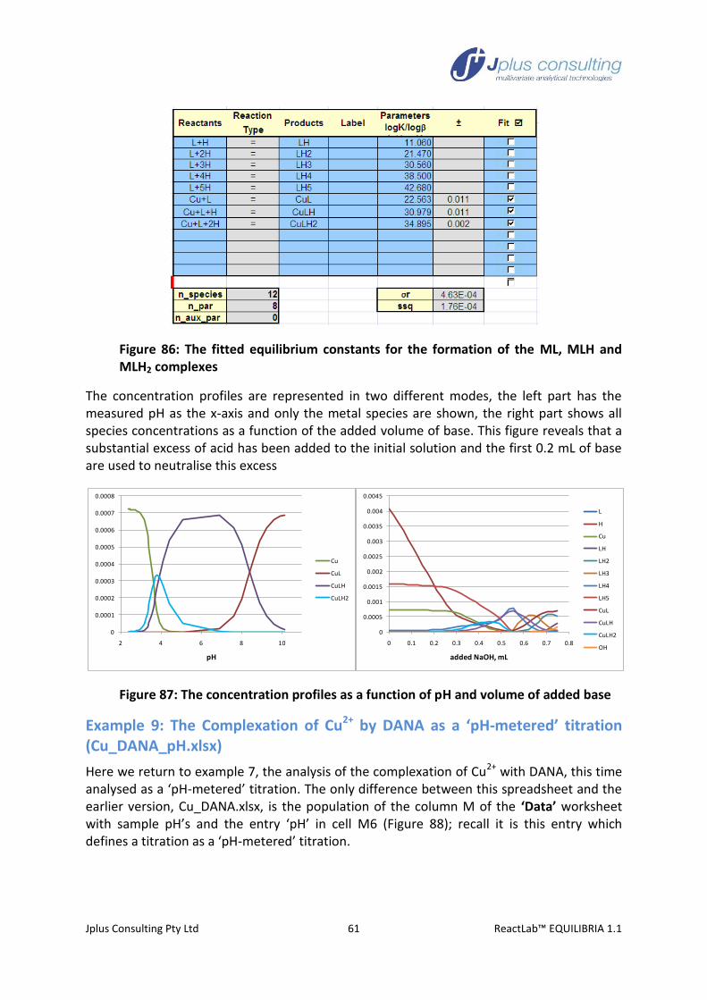
Jplus Consulting Pty Ltd 61 ReactLab™ EQUILIBRIA 1.1
Figure 86: The fitted equilibrium constants for the formation of the ML, MLH and MLH2 complexes
The concentration profiles are represented in two different modes, the left part has the measured pH as the x-axis and only the metal species are shown, the right part shows all species concentrations as a function of the added volume of base. This figure reveals that a substantial excess of acid has been added to the initial solution and the first 0.2 mL of base are used to neutralise this excess
Figure 87: The concentration profiles as a function of pH and volume of added base
Example 9: The Complexation of Cu2+ by DANA as a ‘pH-metered’ titration (Cu_DANA_pH.xlsx)
Here we return to example 7, the analysis of the complexation of Cu2+ with DANA, this time analysed as a ‘pH-metered’ titration. The only difference between this spreadsheet and the earlier version, Cu_DANA.xlsx, is the population of the column M of the ‘Data’ worksheet with sample pH’s and the entry ‘pH’ in cell M6 (Figure 88); recall it is this entry which defines a titration as a ‘pH-metered’ titration.
0
0.0005
0.001
0.0015
0.002
0.0025
0.003
0.0035
0.004
0.0045
0 0.1 0.2 0.3 0.4 0.5 0.6 0.7 0.8
added NaOH, mL
L
H
Cu
LH
LH2
LH3
LH4
LH5
CuL
CuLH
CuLH2
OH
0
0.0001
0.0002
0.0003
0.0004
0.0005
0.0006
0.0007
0.0008
2 4 6 8 10
pH
Cu
CuL
CuLH
CuLH2

Jplus Consulting Pty Ltd 62 ReactLab™ EQUILIBRIA 1.1
Figure 88: The ‘Data’ sheet contains both the original [H]tot values in column F and for the measured pH values in column M.
The results of this analysis are of course essentially identical, compare Figure 89 with Figure 80. The only significant difference is that the standard deviations of the parameters are clearly smaller in the pH-mode.
Figure 89: The resulting constants and their standard deviations for the Cu-DANA system in ‘pH-metered’ titration mode.
The total concentrations of the protons in column F of the ‘Data’ worksheet are ignored in this analysis. Interestingly, if the total concentrations are known, as in this example, they can be compared with those calculated from the concentrations of all proton containing species (in this example it is the sum over the species concentrations H+LH+2LH2-CuLOH-2CuL(OH)2-OH). Figure 90 demonstrates that the difference of course is not zero but insignificant. This can be a valuable test for the correctness of a particular analysis.
Figure 90: Plot of the difference between the total concentrations of protons calculated from the dilutions (column F) and calculated from all species concentrations.
-4.00E-05
-3.50E-05
-3.00E-05
-2.50E-05
-2.00E-05
-1.50E-05
-1.00E-05
-5.00E-06
0.00E+00
5.00E-06
1.00E-05
1.50E-05
2.0 4.0 6.0 8.0 10.0 12.0
Jplus Consulting Pty Ltd 63 ReactLab™ EQUILIBRIA 1.1
References
Marcel Maeder, Yorck-Michael Neuhold. Practical Data Analysis in Chemistry, Elsevier 2007
Equilibria
Arthur Martell, Robert Hancock. Metal Complexes in Aqueous Solutions (Modern Inorganic Chemistry). Springer 1996
Arthur Martell, Ramunas J. Motekaitis. The Determination and Use of Stability Constants. (2nd Edition). Wiley 1992
Juergen Polster, Heinrich Lachmann. Spectrometric Titrations: Analysis of Chemical Equilibria. VCH 1989
Kenneth A. Connors. Binding Constants: The Measurement of Molecular Complex Stability. Wiley 1987
M.T. Beck, I. Nagypal. The Chemistry of Complex Equilibria. Van Nostrand- Reinhold. London 1970
Fitting
Philip R. Bevington, D. Keith. Robinson. Data Reduction and Error Analysis (3rd edition). McGrawHill New York 2002
Meloun Milan, Jiri Militky, and Michele Forina. Chemometrics for Analytical Chemistry (Vol I+II). Ellis Horwood 1994
Peter Gans. Data Fitting in the Chemical Sciences by the Method of Least Squares. Wiley 1992
William H. Press, Brian P. Flannery, Saul A. Teukolsky, and William T. Vetterling. Numerical Recipes in C: The Art of Scientific Computing (2nd edition). Cambridge 1996
E. Joseph Billo. Excel for Chemists: A Comprehensive Guide (2nd edition). Wiley-VCH 2001