1

Equation-free analysis of two-component system signallingmodel reveals the emergence of co-existing phenotypes in theabsence of multistationarityRebecca B. Hoyle1,∗, Daniele Avitabile2, Andrzej M. Kierzek3

1 Department of Mathematics, University of Surrey, Guildford, Surrey GU2 7XH, U.K.2 School of Mathematical Sciences, University of Nottingham, University Park,Nottingham NG7 2RD, U.K.3 Division of Microbial Sciences, University of Surrey, Guildford, Surrey GU2 7XH, U.K.∗ E-mail: r.hoyle@surrey.ac.uk

Abstract

Phenotypic differences of genetically identical cells under the same environmental conditions have beenattributed to the inherent stochasticity of biochemical processes. Various mechanisms have been sug-gested, including the existence of alternative steady states in regulatory networks that are reached bymeans of stochastic fluctuations, long transient excursions from a stable state to an unstable excitedstate, and the switching on and off of a reaction network according to the availability of a constituentchemical species. Here we analyse a detailed stochastic kinetic model of two-component system signallingin bacteria, and show that alternative phenotypes emerge in the absence of these features. We perform abifurcation analysis of deterministic reaction rate equations derived from the model, and find that theycannot reproduce the whole range of qualitative responses to external signals demonstrated by directstochastic simulations. In particular, the mixed mode, where stochastic switching and a graded responseare seen simultaneously, is absent. However, probabilistic and equation-free analyses of the stochasticmodel that calculate stationary states for the mean of an ensemble of stochastic trajectories reveal thatslow transcription of either response regulator or histidine kinase leads to the coexistence of an approxi-mate basal solution and a graded response that combine to produce the mixed mode, thus establishing itsessential stochastic nature. The same techniques also show that stochasticity results in the observationof an all-or-none bistable response over a much wider range of external signals than would be expectedon deterministic grounds. Thus we demonstrate the application of numerical equation-free methods to adetailed biochemical reaction network model, and show that it can provide new insight into the role ofstochasticity in the emergence of phenotypic diversity.

Author Summary

It is a surprising fact that genetically identical bacteria, living in identical conditions, can develop incompletely different ways: for example, one subpopulation might grow very fast and another very slowly.These different phenotypes are thought to be one reason why bacteria that cause disease can survive an-tibiotic treatment or become persistent. This diversity of behaviour is usually attributed to the existenceof multiple stable phenotypic states, or to the coexistence of one stable state with another unstable ex-cited state, or finally to the possibility of the whole biochemical system that controls the phenotype beingswitched on and off. In this paper we describe a different scenario that leads to phenotypic diversity intwo-component system signalling, a very common mechanism that bacteria use to sense external signalsand control their response to changes in their environment. We use probability theory and equation-freecomputational analysis to calculate the average number of molecules of each chemical species presentin the two-component system and hence show that sporadic production of either of two key chemicalcomponents required for signalling can delay the response to the external signal in some bacterial cellsand so lead to the emergence of two distinct cell populations.

2

Introduction

Phenotypic heterogeneity in populations of genetically identical (isogenic) cells is one of the major dis-coveries resulting from a systems approach to molecular and cell biology. Application of single cellimaging techniques has demonstrated that individual cells in clonal populations may have very differentphenotypes under the same environmental conditions [1] and that a pre-existing subpopulation of cellsmay survive a sudden environmental change that is lethal to the majority of cells, such as antibiotictreatment, thus gaining advantage [2]. These observations are particularly important in the context ofsurvival strategies of bacterial pathogens. The phenotypic heterogeneity of isogenic bacterial populationshas been implicated in the emergence of persistence and latent infection in Mycobacterium tuberculosis

that makes this bacterium one of the most dangerous pathogens of mankind [3–5].Phenotypic differences of genetically identical cells under the same environmental conditions have

been attributed to the inherent stochasticity of biochemical processes [6]. According to theoretical pre-dictions elementary chemical reactions involved in biochemical processes exhibit substantial stochasticfluctuations when low numbers of reactant molecules are involved within the small volume of a livingcell. The existence of significant stochastic fluctuations in biochemical processes has been confirmed bynumerous experiments including tracking of individual protein molecules in individual cells in gene ex-pression processes [7]. The mechanism by which these fluctuations give rise to phenotypic diversity hasbeen a subject of intensive study. In most cases phenotypic diversity has been attributed to stochasticfluctuations that result in switching between different stable states of the dynamical system occurring ina network that involves positive feedback loops [2, 8–10]. Alternatively, a network may exhibit excitabledynamics, where fluctuations can lead to transient excursions from a single stable state to an unstable,but slowly decaying, excited state [11,12]. Yet another mechanism arises when a single stable state existsin the system, and the reaction network is effectively switched on and off according to the availability ofone of the constituent chemical species [13,14]. Here we describe a novel situation, in which a monostableor bistable two-component system supports a persistent approximate basal solution, owing to stochasticdelays in the transcription of either histidine kinase or response regulator genes. However, once a par-ticular cell has reached a fully induced level of gene expression there is a negligible chance that it willrevert to the basal state.

Two-component signal transduction systems (TCS) are a very common mechanism by which bacte-ria sense external signals and induce the expression of genes that govern the response to environmentalchange. A particular environmental signal activates a specific membrane-bound histidine kinase (HK),which in turn activates its partner response regulator (RR) via phosphoryl donation. The response regu-lator itself activates the transcription of multiple genes whose products enable the bacterium’s adaptiveresponse to the change it has sensed. A common experimental design is to introduce a reporter genewhose transcription is controlled by the response regulator, and to monitor the TCS output by mea-suring the number of reporter protein molecules produced by the reporter gene. We shall do the samein the numerical and analytical studies we present in this paper. We will later consider two scenarios:autoregulation of the RR gene, where RR activates its own transcription and so positive feedback ispresent, and the constitutively expressed RR gene, where activated transcription of RR is absent. It hasalready been shown that stochastic fluctuations in the expression of RR and HK genes lead to populationheterogeneity with respect to the expression level of genes regulated by the TCS. Sureka et al. [3] usedflow cytometry to show that the MprA/MprB TCS in Mycobacterium smegmatis leads to heterogeneousactivation of the stringent response regulator Rel. that permits persistence to develop in Mycobacterium

tuberculosis [4, 5]. Sureka et al. complemented their experimental observations with numerical simula-tions of a stochastic kinetic model of the TCS, demonstrating that autoregulation of the RR results inbistable behaviour and that stochastic fluctuations in gene expression switch the system between the twostable states corresponding to two different phenotypes. Zhou et al. [7] had earlier used flow cytometry tomeasure gene expression in single Escherichia coli cells from a genetically identical population, in order tostudy cross-activation of the RR PhoB by noncognate HKs in the PhoR/PhoB TCS, and found a bimodal

3

pattern of fluorescent protein reporter gene expression. Subsequently, Kierzek et al. [15] built the mostcomprehensive stochastic kinetic model of two-component system signalling published to date and useddata of Zhou et al. to show that their model reproduces flow cytometry distributions of TCS-regulatedfluorescent protein reporter gene expression. Further computer simulations demonstrated two responsemodes of the TCS leading to population heterogeneity. In the ‘all-or-none’ response that arises when theRR gene is positively autoregulated, the reporter gene is expressed either at fully induced or at basallevel, and a change in the external signal strength results in a corresponding change in the fractions ofcells expressing the gene at basal and fully induced level. Alternatively, population heterogeneity can beobserved in a ‘mixed mode’ that occurs when the RR gene is constitutively expressed. In this responsemode one population of cells expresses the gene at basal level, while in another cell population the geneis expressed at a level that depends on the signal strength. The mixed mode thus combines features ofall-or-none and graded responses.

In this work we use deterministic, probabilistic and equation-free methods to analyse the potentialfor simultaneous coexistence of different phenotypes in the Kierzek, Zhou and Wanner stochastic kineticmodel of TCS signalling [15] (hereafter KZW). The application of equation-free methods to biochemicalreaction networks has typically focused on simple models of small networks [16, 17], though there havebeen some studies of larger scale networks [18–20]. Here we apply them for the first time, to the best ofour knowledge, to a detailed model of signal transduction processes. Our results show that populationheterogeneity can be generated by a molecular interaction network even when it is not multistationary.A deterministic bifurcation analysis of reaction rate equations derived from the KZW stochastic kineticmodel shows that the mixed mode is absent in this framework. However, an equation-free analysis of thestochastic model, using the Gillespie algorithm with tau-leaping as a black-box time-stepper, in orderto find stationary states for the mean of an ensemble of stochastic trajectories, reveals the long-termpersistence of an approximate basal solution that combines with the graded response to produce themixed mode. This confirms the results of a probabilistic analysis that establishes the essential stochasticnature of the mixed mode. The same techniques also show that stochasticity results in the observationof the all-or-none bistable response over a much wider range of external signals than would be expectedon deterministic grounds. In summary, our work uses a detailed mechanistic model of the major signaltransduction and gene regulation mechanism to show that multistationarity and positive feedback arenot necessary for the emergence of phenotypic diversity and that deterministic bifurcation analysis is notalways sufficient to explain phenotypic switching.

In the Results section we first introduce the stochastic kinetic model that we shall be analysing,then we analyse the deterministic reaction rate equations that govern the chemical concentrations inthe thermodynamic limit, and show that these do not permit a mixed-mode solution. In the followingsubsection we analyse the discrete stochastic system using equations for the expected (probabilistic mean)number of molecules of each chemical species present, and show that slow transcription of either or bothof the histidine kinase or response regulator genes can lead to persistence of reporter gene expression ata level that is approximately basal when it would not be expected on deterministic grounds. In the finalsubsection of Results we show that equation-free methods can locate this unexpected basal expressionsolution and investigate its stability using only direct stochastic simulations. Thus we confirm the findingsof our probabilistic analysis, and also demonstrate the potential of equation-free methods to shed lighton stochastic effects in large complex systems where a probabilistic analysis is too difficult to perform.In the Discussion we summarise our findings and highlight their biological significance. The Methodssection includes mathematical details of the probabilistic and equation-free analyses.

4

Results

Stochastic kinetic model

We base our stochastic kinetic model of the PhoBR TCS in E. coli on that of Kierzek, Zhou andWanner [15], summarised in Fig. 1. (A detailed representation of the model in Systems Biology GraphicalNotation (SBGN) is given in [15].) We are interested in stochastic switching of reporter gene expression,and hence in the numbers of reporter protein molecules produced. The external signal is modelled asthe ratio of the HK autophosphorylation to dephosphorylation rates. Dashed arrows on the diagramindicate activated transcription of the response regulator and reporter genes, modelled using the Shea-Ackers formalism [21], where the reaction rate increases with the concentration of phosphorylated RR,saturating for large [RRP] at a level much higher than in the absence of RRP. As mentioned above, wewill consider two cases: the autoregulated and the constitutively expressed RR gene. Transcription andtranslation of the response regulator, histidine kinase and reporter genes are modelled as pseudo-first-order reactions. The circle-headed arrows indicate HK/RR complexes in phosphate transfer processes,according to the Batchelor & Goulian model [22]. Included in our model but not shown in the diagramare dimer formation and dissociation and also reporter protein and mRNA degradation.

KZW simulated the reaction network using the Gillespie algorithm [23] for direct stochastic sim-ulation, and incorporating gene replication and cell division events. The Gillepsie algorithm updatesthe number of molecules Xk(t) of the kth chemical species, using the propensity functions aj(X(t)),where aj(X(t))dt is the probability that the jth reaction takes place in the time interval [t, t + dt),and its associated stochiometric vector νj whose kth component is the change in Xk caused by the jthreaction. The propensity functions for the reactions involved in the KZW model are given in Table 1,where X1, X2, . . . , X12 are the numbers of molecules of phosphorylated RR protein (RRP), mRNA of RR(mRNA-RR), RR protein (RR), HK protein (HK), phosphorylated HK dimer (HK2P), complex of RRand phosphorylated HK dimer (RR-HK2P), complex of phosphorylated RR and HK dimer (RRP-HK2),mRNA of reporter (mRNA-Rep), reporter protein (Rep), mRNA of HK (mRNA-HK), phosphorylatedRR dimer (RR2P) and HK dimer (HK2) respectively, and x1, x2, . . . , x12 are the corresponding concentra-tions. The correspondence between chemical species and model variables is also given in Table 2 for easeof reference. The parameters c1 to c24 given in Table 1 were chosen by KZW to accord with experimentaldata where available, or with validated models of prokaryotic gene expression or, in cases where it didnot affect the qualitative results, they were chosen at will [15]. The concentration of RNA polymerase(RNAP) is fixed, at α0 = 30/V NA, in order to model transcription and translation as pseudo-first-orderreactions, following KZW [15], where V is the cell volume and NA is the Avogadro constant and weset V NA = 109. The concentrations of the various degradation products mentioned in Table 1 do notinfluence the propensity functions and so we do not include them as variables in our model. The externalsignal is modelled as the ratio of the autophosphorylation to dephosphorylation rates for histidine kinase,c14/c15, which we vary by keeping c14 fixed and changing c15.

In summary, the Gillepsie algorithm consists of randomly selecting the next reaction that occurs to bej with probability proportional to aj(X(t)), and randomly selecting the time, τ , until that next reactiontakes place from an exponential distribution with rate parameter

∑

j aj(X(t)). The vector X is updatedaccording to the numbers of molecules created and consumed in reaction j, and time is increased byt → t + τ [24]. Stepping forward in time in this way gives a single realisation of the system. Typically,many realisations are computed to give a fuller picture of the system behaviour. KZW started eachrealisation at X = 0 at time t = 0, and performed 10,000 realisations, each of 20,000s duration, for eachparameter combination of interest.

KZW were interested in two sets of comparisons: autoregulation of the RR gene versus constitutiveexpression, as discussed above, and fast versus slow transcription of HK. KZW chose an operating pointfor their system such that the mean steady state numbers of RR and HK protein molecules were 3800 and25 respectively. The parameter values given in Table 1 are those for the autoregulated, slow transcription

5

case. To simulate a constitutively expressed response regulator gene, we break the feedback loop byreplacing the first two response regulator transcription reactions in Table 1 by the reaction prom-RR →mRNA-RR+prom-RR, where prom-RR is the promoter region of the RR gene, with propensity functionc25, where the rate constant c25 is chosen to lead to the same system operating point in order to permit faircomparison with the autoregulated case. KZW found that a value of c25 = 0.04125 accomplished this [15].In order to isolate the effect of variability in HK expression, KZW fixed the overall rate of transcriptionfollowed by translation to be c6c7 = 3× 10−5s−1. In the slow transcription, fast translation case the rateconstants were c6 = 10−4s−1 and c7 = 0.3s−1, while in the fast transcription, slow translation case thesevalues were swapped. Slow transcription followed by fast translation produces HK in bursts, while fasttranscription and slow translation leads to more continuous production [15].

With autoregulation of the RR gene and fast transcription of HK (Fig. 2a) KZW saw stochasticswitching between the basal and fully induced levels of reporter gene expression - a so-called ‘all ornone’ response. In other words, some trajectories showed very little reporter protein present at timet = 20, 000s, while some showed a large amount, and the number of reporter protein molecules producedduring the productive trajectories did not seem to depend strongly on the external signal strength. Thepicture was similar with autoregulation and slow HK transcription, but there were fewer realisations atthe activated level (Fig. 2b). In the case of a constitutively expressed RR gene and fast HK transcription,there was no stochastic switching - a graded response was seen instead, where the number of reporterprotein molecules produced increased with increasing signal strength (Fig. 2c). An interesting novel casewas found when the RR gene was constitutive, but transcription was slow, when stochastic switching anda graded response were seen simultaneously - a so-called ‘mixed mode’ (Fig. 2d). It is the unexpectedexistence of this mixed mode that we seek to explain through our analyses below.

Reaction rate equations and deterministic bifurcation analysis

In the thermodynamic limit where the cell volume and the numbers of molecules of each chemical speciestend to infinity, but the concentration of each species remains constant [24], the KZW model for thesystem containing an autoregulated RR gene can be reduced to the following set of deterministic reaction

6

rate equations that describe mass-action kinetics for continuous real-valued concentrations:

dx1

dt= −k5x1 − 2k24x

21 + 2k23x11 − k12x1x12 + k11x6, (1)

dx2

dt=

k2K1α0 + k1K2α0x11

1 +K2α0x11 +K1α0 +K3x11− k4x2, (2)

dx3

dt= k3x2 − k5x3 − k10x3x5 + k13x7, (3)

dx4

dt= −k9x4 − 2k22x

24 + 2k21x12 + k7x10, (4)

dx5

dt= −k10x3x5 + k14x12 − (k9 + k15)x5, (5)

dx6

dt= k10x3x5 − k11x6, (6)

dx7

dt= k12x1x12 − k13x7, (7)

dx8

dt=

k17K1α0 + k16K2α0x11

1 +K2α0x11 +K1α0 +K3x11− k19x8, (8)

dx9

dt= k18x8 − k20x9, (9)

dx10

dt= k6 − k8x10, (10)

dx11

dt= k24x

21 − (k23 + k5)x11, (11)

dx12

dt= −k12x1x12 + k22x

24 − (k21 + k9 + k14)x12 + k15x5 + k11x6 + k13x7.

(12)

If the RR gene is constitutively expressed, then equation (2) becomes

dx2

dt= k25 − k4x2. (13)

The deterministic rate constants are appropriately scaled versions [24] of those used in the stochas-tic kinetic model: ki = ci for i = 3, 4, 5, 7, 8, 9, 11, 13, 14, 15, 18, 19, 20, 21, 23, ki = ci/(V NA) for i =1, 2, 6, 16, 17, 25, ki = ciV NA for i = 10, 12, 22, 24.

In reality for this system some species remain low in number, fluctuating between zero and a smallinteger number. Thus we expect the deterministic continuous analysis based on these equations to giveclues as to the system behaviour, but to fail to describe it adequately in some important respects.

Note that equations (8) and (9) decouple from the rest of the system, being dependent only on theinput value of x11, but not feeding back into the remaining equations through the values of x8 and x9.Thus the reporter protein concentration, x9, is ultimately determined by that of the phosphorylated RRdimer, x11.

We considered four sets of parameter values that gave every combination of fast and slow transcriptionwith autoregulated and constitutively expressed RR gene. In each case we first found a stationary solutionof the reaction rate equations for a particular value of the external signal (k14/k15 = 0.1) numericallyand then continued it over a range of external signals k14/k15, where k15 was varied, using the XPPAUTsoftware package [25] to produce a deterministic bifurcation diagram.

In the autoregulated case, the basal level of reporter gene expression is shown at zero external signal

7

(k14 = 0), where it corresponds to the following fixed point of equations (1)-(12):

x1 = x5 = x6 = x7 = x11 = 0, (14)

x10 = k6/k8 (15)

x2 =k2κ1α0

k4(1 + κ1α0)≡ x20, (16)

x3 =k3k5

x20, (17)

x8 =k17κ1α0

k19(1 + κ1α0)≡ x80, (18)

x9 =k18k20

x80, (19)

x4 = −k21 + k94k22

(

1−

√

1 +

(

8k22k21 + k9

)

k6k7k8k9

)

≡ x40, (20)

x12 =1

2

(

k6k7k8k9

− x40

)

. (21)

More generally it can be shown that the fixed points of equations (1)-(12) are given by

x11 =k24x

21

k23 + k5, (22)

x2 =(k2K1 + k1K2x11)α0

k4(1 +K2α0x11 +K1α0 +K3x11), (23)

x10 =k6k8

, (24)

x12 =1

2k21

(

k9x4 + 2k22x24 −

k6k7k8

)

, (25)

x7 =k12k13

x1x12, (26)

x8 =(k17K1 + k16K2x11)α0

k19(1 +K2α0x11 +K1α0 +K3x11), (27)

x9 =k18k20

x8, (28)

x5 = −k22k21

x24 −

k9 + k212k21

(

x4 −k6k7k8k9

)

, (29)

x6 =k14k11

x12 −k9 + k15

k11x5, (30)

x3 =k11x6

k10x5, (31)

8

where x1 and x4 are the solutions of the nonlinear equations

0 =1

2

(

k9 + k15 +k9k21

(k9 + k15 + k14 − k12x1)

)(

x4 −k6k7k8k9

)

−k5x1 −2k5k24x

21

k23 + k5+

k22k21

(k9 + k15 + k14 − k12x1)x24, (32)

0 = k10

(

−k22k21

x24 −

1

2k21(k9 + k21)

(

x4 −k6k7k8k9

))

×

k3

(

k2K1α0 + k1K2α0k24x

21

k23+k5

)

k4

(

1 +K1α0 + (K2α0 +K3)k24x

21

k23+k5

) − k5x1 −2k5k24x

21

k23 + k5

−k5

(

k5x1 +2k5k24x

21

k23 + k5+

k22k21

k12x1x24

)

. (33)

In the constitutive case, equations (16) and (23) become x2 = k25/k4 and equation (33) becomes

0 = k10

(

−k22k21

x24 −

1

2k21(k9 + k21)

(

x4 −k6k7k8k9

))(

k3k25k4

− k5x1 −2k5k24x

21

k23 + k5

)

−k5

(

k5x1 +2k5k24x

21

k23 + k5+

k22k21

k12x1x24

)

. (34)

It is clear that, apart from the value of x10, the steady solutions depend on the rates of HK translationand transcription only through the product k6k7, which we have set to be constant. Thus the slowand fast transcription cases have the same fixed points in the deterministic framework. It turns outthat these fixed points also have the same stability type over the range of external signals that weexamined, and so the deterministic bifurcation diagrams are the same for fast and slow transcription. Theautoregulated case (Fig. 3a) shows a classical bistable scenario, with a stable state corresponding to thebasal level of expression of reporter protein, coexisting over a range of external signals (4.529 × 10−4 ≤k14/k15 ≤ 6.323 × 10−3), with a stable state corresponding to the activated level of expression. Fork14/k15 < 4.529 × 10−4 only the basal expression solution exists, while for k14/k15 > 6.323 × 10−3 onlythe activated state is possible. The switch between these two states, gives a classical ‘all-or-none’ response:in a population of cells, for a given external signal, some will show activated expression of reporter proteinand some will show only basal level expression. This case corresponds to Figs. 2a (fast transcription) and2b (slow transcription) of the KZW results, where an ‘all-or-none’ response is indeed seen. On breakingthe feedback loop to investigate the constitutively expressed RR gene, a graded response is seen (Fig.3b), where the amount of reporter protein produced rises steadily as the external signal is increased, andthis solution is stable. Both Figs. 2c and d show KZW results using a constitutively expressed RR gene,but while they saw a graded response in the fast transcription case (Fig. 2c) they saw a mixed modewhen transcription was slow (Fig. 2d), where the basal level of reporter gene expression persists for atleast 20,000s in some cells even for quite large external signals. In our deterministic bifurcation analysis,this basal solution is absent and so there is no mixed mode. We deduce that the mixed mode resultsfrom stochasticity and/or discreteness.

Analysis of the discrete stochastic model

We want to find the approximate steady state of the discrete stochastic system. It does not have truefixed points, such that X(t) remains constant for all time. However, we can look for fixed points of the

9

expected value, or mean, 〈X〉. As shown in Methods, 〈X〉 evolves according to the differential equation

d〈X〉

dt=

M∑

j=1

νj〈aj(X)〉. (35)

This is different from the reaction rate equations for the evolution of the vector of concentrations x

because < aj(X) > 6= aj(< X >) in general for nonlinear aj(X) [24]. Thus when the RR gene isautoregulated, the rates of change of the components 〈Xk〉 of the mean are

d〈X1〉

dt= −c5〈X1〉 − 2c24〈X1(X1 − 1)〉+ 2c23〈X11〉

−c12〈X1X12〉+ c11〈X6〉, (36)

d〈X2〉

dt=

⟨

c2κ1α+ c1κ2αX11

1 + κ2αX11 + κ1α+ κ3X11

⟩

− c4〈X2〉, (37)

d〈X3〉

dt= c3〈X2〉 − c5〈X3〉 − c10〈X3X5〉+ c13〈X7〉, (38)

d〈X4〉

dt= −c9〈X4〉 − 2c22〈X4(X4 − 1)〉+ 2c21〈X12〉

+c7〈X10〉, (39)

d〈X5〉

dt= −c10〈X3X5〉+ c14〈X12〉 − (c9 + c15)〈X5〉, (40)

d〈X6〉

dt= c10〈X3X5〉 − c11〈X6〉, (41)

d〈X7〉

dt= c12〈X1X12〉 − c13〈X7〉, (42)

d〈X8〉

dt=

⟨

c17κ1α+ c16κ2αX11

1 + κ2αX11 + κ1α+ κ3X11

⟩

− c19〈X8〉, (43)

d〈X9〉

dt= c18〈X8〉 − c20〈X9〉, (44)

d〈X10〉

dt= c6 − c8〈X10〉, (45)

d〈X11〉

dt= c24〈X1(X1 − 1)〉 − (c23 + c5)〈X11〉, (46)

d〈X12〉

dt= −c12〈X1X12〉+ c22〈X4(X4 − 1)〉 − (c21 + c9 + c14)〈X12〉

+c15〈X5〉+ c11〈X6〉+ c13〈X7〉, (47)

where α = α0V NA, κ1 = K1/(V NA), κ2 = K2/(V NA)2 and κ3 = K3/(V NA). If the RR gene is

constitutively expressed, then equation (37) becomes

d〈X2〉

dt= c25 − c4〈X2〉. (48)

To look for a basal solution for these equations, we set c14 = 0 for a zero external signal, and lookfor solutions 〈X〉 = X(b) such that d〈X〉/dt|〈X〉=X(b) = 0. In Methods, we show that 〈f(X)〉|〈Xj〉=0 =

〈f(X|Xj=0)〉. Bearing this in mind, we find that the basal solution for the means satisfies X(b)1 = X

(b)5 =

10

X(b)6 = X

(b)7 = X

(b)11 = 0,

X(b)2 =

c2κ1α

c4(1 + κ1α), (autoregulated), (49)

X(b)2 =

c25c4

, (constitutive), (50)

X(b)3 =

c3c5

X(b)2 , (51)

X(b)8 =

c17κ1α

c19(1 + κ1α), (52)

X(b)9 =

c18c20

X(b)8 , (53)

X(b)10 =

c6c8

, (54)

and that X(b)4 and X

(b)12 correspond to fixed points (if such can be found) of the equations

d〈X4〉

dt= −c9〈X4〉 − 2c22〈X4(X4 − 1)〉+ 2c21〈X12〉

+c6c7c8

, (55)

d〈X12〉

dt= c22〈X4(X4 − 1)〉 − (c21 + c9)〈X12〉. (56)

These last two equations are not in closed form, involving the higher-order moment 〈X24 〉, and so we

cannot deduce from them whether a solution for X(b)4 and X

(b)12 actually exists. If the basal solution

does exist, then we see that, with the exception of the values of X(b)4 and X

(b)12 it is the equivalent of the

deterministic basal solution with the deterministic rate constants replaced by their stochastic equivalents.In order to understand the stochastic behaviour, the equations for the evolution of the mean are not

sufficient. For a given realisation of the system, the Xi must take non-negative integer values, and thisdiscreteness turns out to be important in understanding the existence of basal solutions where they arenot predicted by the mass-action or mean reaction rate equations. We have 〈X10〉 = c6/c8 from equation(45). In the case of slow transcription, where [c6/c8] = 0 (and where here and hereafter [ ] indicates therounded value, with half integers being rounded upwards), the closest an individual trajectory can get tothe fixed point of the mean is at X10 = 0. We can now look for fixed points of 〈X〉|X10=0, which satisfyequations (36)-(44), (46) and (47), with the term involving 〈X10〉 being zero in equation (39). In fact, inthe slow transcription case we have d〈X10〉/dt|X10=0 = 10−4s−1 and so if we can find a steady state forthe remaining components of 〈X|X10=0〉, we would expect it to persist over a timescale of approximately104s.

Equations (43) and (44) show that the basal level of reporter protein production occurs when X11 = 0,in other words when no phosphorylated HK dimer (HK2P) is present, so we will look for a steady state

solution 〈X|X10=0〉 that also has 〈X11〉 = 0 and call it X(s). Thus we have X(s)10 = X

(s)11 = 0, and

we now look for values of the remaining components of X(s) that are consistent with this. We are no

longer restricting the external signal, c14/c15, to be zero. However, we find X(s)j = X

(b)j for all j except

j = 4, 10, 12 for which X(s)j = 0. Thus an approximate steady state X(s) can be found that corresponds

to a basal level of reporter protein production for arbitrary values of the external signal.For the parameter values used in our study, we find that in the autoregulated slow HK transcription

case X(s) = (0, 5.42 × 10−3, 8.44, 0, 0, 0, 0, 5.42 × 10−1, 8.44 × 102, 0, 0, 0) and in the constitutive slowtranscription caseX(s) = (0, 10.3, 1.61×104, 0, 0, 0, 0, 5.42×10−1, 8.44×102, 0, 0, 0). In both autoregulatedand constitutive cases, these solutions are equivalent to the deterministic and mean basal solutions except

11

for the values ofX4, X10 andX12. Thus we expect to see the basal level of reporter protein in a proportionof cells for all values of the external signal in the slow transcription case for both the constitutivelyexpressed and autoregulated RR gene. In the constitutive case, this is the origin of the mixed mode, andin the autoregulated case it is why the basal solution is seen at unexpectedly high values of the externalsignal.

Note from equation (36) that a requirement for the existence of an approximate discrete basal steadystate with 〈X11〉 = 0 is that 〈X1〉 = 0 and equation (46) shows that this in turn requires that therebe no RR-HK2P complex present (〈X6〉 = 0). Equation (6) then implies we must have 〈X3X5〉 = 0.This holds for the majority of trajectories over long times for both slow transcription cases, since slow

transcription of HK means that the levels of mRNA-HK is typically zero (X(s)10 = 0), and when that is

true we can find steady states where there is no HK protein (X(s)4 = 0) or HK dimer (X

(s)12 = 0) and

hence no phosphorylated HK dimer forms (X(s)5 = 0), as we have just shown.

In the autoregulated cases, if we look for steady state solutions for the mean that have 〈X11〉 = 0,then from equations (37) and (74) we have

〈X2〉 =c2κ1α

c4(1 + κ1α)(57)

and for our parameter values this gives 〈X2〉 = 5.42 × 10−3, which indicates that the average numberof mRNA-RR molecules present is very low and transcription of RR is slow. The closest an individualtrajectory can come to this value is at X2 = 0, so we look for fixed points X(a) ≡ 〈X|X2=0〉, with

X(a)11 = 0, that satisfy equations (36) and (38)-(47) with the left-hand sides equal to zero. If we can

find such a solution, we would expect it to persist over timescales of about 104s (since (d〈X2〉/dt)−1 =

(1 + κ1α)/(c2κ1α) = 4.61 × 104s at 〈X11〉 = 〈X2〉 = 0). Since X(a)2 = 0 (no mMRNA-RR is present),

and since for a basal solution we also have no RR2P (X(a)11 = 0) or RRP (X

(a)1 = 0) and thus no RRP-

HK2 (X(a)7 = 0), we find from equation (38) that it is consistent to have no response regulator protein

(X(a)3 = 0) and so again 〈X3X5〉 = 0 is satisfied. Thus in the autoregulated, fast HK transcription case

we find the approximate basal solution X(a) such that X(a)2 = 0, X

(a)j = X

(b)j for j = 1, 3, 6, 7, 8, 9, 10, 11,

and X(a)4 , X

(a)5 and X

(a)12 correspond to fixed points of the equations

d〈X4〉

dt= −c9〈X4〉 − 2c22〈X4(X4 − 1)〉+ 2c21〈X12〉

+c6c7c8

, (58)

d〈X5〉

dt= c14〈X12〉 − (c9 + c15)〈X5〉, (59)

d〈X12〉

dt= c22〈X4(X4 − 1)〉 − (c21 + c9 + c14)〈X12〉

+c15〈X5〉, (60)

if they exist. (Again these equations involve the second order moment 〈X24 〉, and so we cannot deduce

from them the existence of a fixed point of the mean.)

For the parameter values of our study this gives X(a) = (0, 0, 0, X(a)4 , X

(a)5 , 0, 0, 5.42 × 10−1, 8.44 ×

102, 75, 0, X(a)12 ) for the autoregulated fast transcription case. Although the terms in 〈X2

4 〉 prevent us

from determining X(a)4 , X

(a)5 and X

(a)12 explicitly, we see that

c14〈X12〉 − (c9 + c15)〈X5〉 = 0, (61)

〈X4〉+ 2〈X5〉+ 2〈X12〉 =c6c7c8c9

, (62)

12

and hence, assuming that the solution does indeed exist, we must have

X(a)5 =

c142(c9 + c14 + c15)

{

c6c7c8c9

−X(a)4

}

, (63)

X(a)12 =

c9 + c152(c9 + c14 + c15)

{

c6c7c8c9

−X(a)4

}

, (64)

where X(a)4 is chosen such that

{

c6c7c8c9

− 〈X4〉

}{

c9 +c21(c9 + c15)

c9 + c14 + c15

}

− 2c22〈X4(X4 − 1)〉 = 0 (65)

holds.Since 〈X2

4 〉 ≤ 〈X4〉2, X

(a)4 must satisfy

{

c6c7c8c9

−X(a)4

}{

c9 +c21(c9 + c15)

c9 + c14 + c15

}

− 2c22

{

(X(a)4 )2 −X

(a)4

}

≤ 0. (66)

For the parameter values just mentioned this gives X(a)4 ≥ 5.59, and from equations (63) and (64) we

then see that X(a)5 ≤ 50.5 and X

(a)12 ≤ 5.12. Since 〈X2

4 〉 ≥ 0, we must also have

{

c6c7c8c9

−X(a)4

}{

c9 +c21(c9 + c15)

c9 + c14 + c15

}

+ 2c22X(a)4 ≥ 0. (67)

This is automatically satisfied if X(a)4 ≤ c6c7/c8c9, which is required if equations (63) and (64) are to

have non-negative solutions for X(a)5 and X

(a)12 .

Note that in the autoregulated, slow HK transcription case, we can find an approximate basal solution

X(as) that has both X(as)2 and X

(as)10 equal to zero: in other words X

(as)j = X

(s)j for j = 1, 4, . . . , 12 and

X(as)2 = X

(as)3 = 0, with the growth rates of all components being zero except for X

(as)2 and X

(as)10 where

the growth rates are 4.125 × 10−2s−1 and 10−4s−1 respectively. For the parameter values of our studywe have X(as) = (0, 0, 0, 0, 0, 0, 0, 5.42 × 10−1, 8.44× 102, 0, 0, 0).

In the case of the constitutively expressed RR gene with fast HK transcription, no approximate basalsteady state can be found. The rapid production of mRNA-HK (X10) in the fast transcription cases- a steady state of approximately [c6/c8] = 75 molecules from equation (45) - ultimately leads to theproduction of phosphorylated HK dimer (X5). The rate constant, c25, for the constitutively expressedRR gene is chosen to produce similar numbers of reporter protein molecules to those found in an activatedcell in the autoregulated case. Thus, when phosphorylated RR dimer (X11) is scarce, RR transcriptionis much faster for the constitutively expressed than autoregulated gene. Equation (48) gives a steadystate of approximately 10 mRNA-RR molecules in the constitutive cases, since 〈X2〉 = c25/c4 = 10.3,and hence RR protein (X3) is also present at high levels. The combination of both phosphorylated HKdimer and RR protein allows RR-HK2P complex (X6) and hence RR2P (X11) to form and ultimatelyleads to the presence of reporter protein (X9) at levels much higher than basal.

Starting from the approximate basal solutions, we need RR protein (X3), and prior to this mRNAof RR (X2), and HK2P (X5), and prior to this HK protein (X4) to form before reporter protein can be

formed. This will happen only very rarely because either X(a)2 and X

(a)3 are zero (autoregulated cases)

or X(s)4 and X

(s)5 are (slow HK transcription cases) or both (autoregulated slow transcription case) and

the corresponding growth rates are tiny or zero, showing that the reactions involving these species arewell-balanced at X(a), X(s) and X(as). Thus the approximate basal solution is expected to persist overlong times for a significant proportion of trajectories, or equivalently in a significant proportion of cells.

13

Only in the constitutive fast HK transcription case is there the required combination of nonzero X3 (andX2) and X5 (and X4) to cause the production of RR-HK2P complex (X6) and lead within a short timefor the vast majority of trajectories (or cells) to the presence of reporter protein (X9) at levels abovebasal. This is the only case in which the basal solution is not observed for high external signals, as canbe seen from Fig. 2c. Only a graded response is observed.

The results show that slow transcription of either or both of the HK and RR genes can lead tothe persistence of the basal solution where it would not be expected from analysis of the deterministicreaction rate equations. The discrepancy between the deterministic and discrete stochastic models arisesfrom the fact that trajectories do not remain close to the basal level of expression for all time in thestochastic model when the basal solution is not a stable fixed point of the system. Rather they eventuallyapproach the discrete stochastic equivalent of the steady-state solution found in the deterministic model.However, there is a delay before transcription of HK and RR is initiated during which a near zero level ofexpression is observed. HK transcription takes place at a (stochastic) rate c6 to give mRNA-HK, whichis then translated at a rate c7X10, where X10 is the number of mRNA-HK molecules. For fixed c6c7, ifthe transcription rate constant c6 is small, transcription occurs in bursts [15]: it is delayed for a long timein some realisations, followed by very rapid translation when the number of reporter protein moleculesclimbs up quite quickly towards its steady state value. Hence a basal level of expression is observed fora long time in some realisations of the discrete stochastic model. This is the origin of the mixed modeobserved in the constitutive case (Fig. 2d) for slow HK transcription initiation. On the other hand iftranscription is initiated rapidly, corresponding to c6 large, the number of mRNA-HK molecules risesquickly and production of reporter protein occurs more steadily as long as RR is also being transcribedfast enough; thus trajectories depart from the basal solution earlier on average. The basal expressionlevel is therefore not observed over long periods (Fig. 2c). Note that the overall rate of transcriptionand translation of HK is the same in both cases, namely c6c7X10. If RR is transcribed slowly then thiscan also result in the basal expression level being observed over long periods, even if HK is transcribedrapidly, and this is why we see a persistent basal solution in the fast HK transcription autoregulatedcase. Bistable behaviour of stochastic origin has also been found in direct stochastic simulations ofautoregulated gene expression [13, 14], where although mRNA transcription and translation are eithernot considered, or treated as a single lumped step, stochastic activation of the gene by binding of aprotein dimer is required before gene expression can proceed. However, in that case, while dimer bindingis sporadic, the remaining biochemical reactions in the network are comparatively fast, so that geneexpression is effectively switched on or off by the presence or absence of the dimer and thus proceeds inbursts. At any given time some cells in a population would be switched off and so a basal expression statewould be found when it was not expected on deterministic grounds, but the mechanism is different fromthe one we see here, where a given cell may persist in a basal state over a long period before transitioningto a higher level of reporter gene expression.

The production of reporter protein at a level above basal, ultimately requires the simultaneous presencein the system of RR (response regulator protein, X3) and HK2P (phosphorylated HK dimer, X5). This ismuch more likely to happen if both are present in significant numbers, as is forced to occur by the formsof the mRNA-HK and mRNA-RR growth rates in the constitutive fast HK transcription case, than ifeither RR or mRNA-HK appears only sporadically, which is true for the former if response regulator isinitially scarce and the gene is autoregulated and the latter if HK transcription is slow. In these cases, weexpect reporter protein production to continue at basal level over long times. As the system is stochasticthere will always be trajectories that do lead to production of reporter protein at much higher levels, andindeed every trajectory would be expected to reach these levels if we were to wait long enough, becauseeventually there would be a stochastic fluctuation large enough to bring the trajectory into the basin ofattraction of the induced expression solution. Since bacteria have a finite lifetime we would in practiceobserve reporter protein production at induced expression levels in a proportion of cells and at basal levels

in the remainder. In the autoregulated slow HK transcription case, both values X(as)3 and X

(as)5 are zero,

14

so it is to be expected that after a given time a smaller fraction of cells in this case produces reporterprotein at induced levels than in the autoregulated fast HK transcription or constitutively expressed slowHK transcription cases, and it can be seen from Fig. 2 that this is indeed the case. In the constitutively

regulated slow HK transcription case, the expected value of X(s)3 (response regulator protein) is very high

at 1.61 × 104, and so RR-HK2P complex (X6) and hence reporter protein (X9) will be formed rapidlyif stochastic fluctuations lead to the presence of a few HK2P molecules (X5). Thus after a fixed lengthof time, we expect a greater fraction of cells to show high levels of reporter protein in the constitutivelyregulated slow HK transcription case than in the fast HK transcription autoregulated case, where nomore than about fifty HK2P molecules are present on average at steady state for the approximate basal

solution (X(a)5 ≤ 50.5), and so production of RR-HK2P complex (X6) will proceed much more slowly

when occasional molecules of response regulator (X3) are formed. Again this confirms what is seen inFig. 2.

Equation-free determination of steady states for the stochastic kinetic model

In the previous subsection we analysed the equations for the time evolution of the mean 〈X〉 directly inorder to find the approximate basal solutions that give rise to the mixed mode and to the extended rangeof signals over which an all-or-none response can be seen. We were fortunate in being able to do this:many reaction networks would be too complicated to succumb to this approach. However, it is possibleto use direct stochastic simulations to gain information about the existence and stability of steady statesof the probabilistic mean. In this subsection we use equation-free techniques to confirm the existenceof the approximate basal solutions and investigate their stability. This approach could be extended tocomplex reaction networks that cannot be analysed explicitly.

So-called ‘equation-free’ methods (see [26–28] and references therein) are used to analyse the behaviourof dynamical systems that are either stochastic, or alternatively, deterministic of high dimension and withrandom initial conditions. The time evolution is obtained by a numerical time-stepping algorithm, andtypically one is interested in characterising the asymptotic behaviour of the probability density functionsof the associated state variables. Evolution equations for the probability distribution are often hard towrite down in closed form, albeit their existence is guaranteed in most cases. However, ensembles ofrealisations of the dynamical system can be obtained by running the time stepper many times over fora given simulation time or time horizon, starting from a probability distribution of initial conditions.From these ensembles of realisations, moments (typically the mean and sometimes also the variance)of the probability distribution of state variables at the end time can be calculated. A key idea behindequation-free methods is that, if the high-order moments evolve much faster than (are slaved to) thelow-order ones, there exists a closed evolution equation for the first few moments of the distribution. Themethod allows for the computation of steady states of, for example, the mean values of state variables,together with the corresponding Jacobian matrix that determines the stability eigenvalues for them, andso a bifurcation diagram can be constructed for these mean values. Thus all the powerful machineryof nonlinear dynamical systems can be brought to bear to explore systems for which explicit governingequations are not available.

Typically the equation-free method also encompasses the identification of fast and slow state variablesand the use of ‘coarse projective iteration’ to speed up the time-stepping in large systems. We have notimplemented these aspects here, in the first case because we did not expect any separation of variablesinto fast and slow to remain valid over the entire range of parameter regimes that we need to investigate,since we are explicitly varying the timescales of interest in this problem, and in the second case becausethe use of modified tau-leaping in the Gillespie algorithm performs a similar role to coarse projectiveiteration.

Equation-free methods have been demonstrated to work well for low-dimensional systems with tunablenoise. They have also been used to examine stochastic simulations of (bio)chemical reaction networks in

15

simple [16,17,29–31] and somewhat more complex cases [18–20]. Here we extend this work, by applyingequation-free techniques to Gillespie algorithm simulations of a realistic biochemical reaction network ofmoderate complexity, which represents a significant computational challenge to the method.

In order to capture the purely stochastic near-zero solutions involved in the mixed mode (constitutiveslow transcription case) and the extension of the basal expression level to high external signals in theautoregulated cases, we use an equation-free method [32] in which the Gillespie algorithm is a black-box time-stepper. We begin by identifying microscopic and macroscopic variables for the system. Themicroscopic variables are contained in the vector X(t), denoting the number of molecules of each speciesat time t. The coarse variables of our problem are then defined as an ensemble average of X(t) over alarge number, N , of realisations of the Gillespie algorithm

Y (t) = limN→∞

1

N

N∑

n=1

X(n)(t), (68)

where X(1)(t), . . . ,X(N)(t) are the values of X(t) found in the realisations 1 to N .A central role in the equation-free framework is played by the coarse time-stepper

Y (t+ th) = Φth(Y (t)). (69)

The operatorΦth evolves the macroscopic state from time t to time t+th and, in general, is not available inclosed form. However, it is possible to advance the coarse variables in time using independent microscopicruns of the Gillespie algorithm. The coarse time-stepper is then composed from these microscopic runsin three stages: lift, evolve and restrict [27] as described in Methods.

Once the coarse time-stepper is defined, we can find steady states Ys of the coarse evolution (69) bycomputing solutions to the equation

Ys −Φth(Ys) = 0. (70)

In our implementation, we find Ys via Broyden’s iterations: function evaluations consist in performing thelift-evolve-restrict steps mentioned above, whereas the Jacobian at points Y is determined numericallyfrom the values of Φth(Y + δY ) for various small perturbations of the mean δY . By choosing the timehorizon, th, appropriately we can pick up metastable solutions that persist, on average, for that lengthof time, but are not true steady states of the system.

In practice, this turns out to be less straightforward than one might wish. The identification of a singlefixed point requires hundreds of thousands to millions of realisations of the Gillespie algorithm (owing tothe use of a large ensemble and the requirement for several iterations of the algorithm before convergence),and is consequently very slow, even when the calculations are parallelised. The error tolerance that canbe achieved depends on the number of realisations in the ensemble, and so there is a trade-off betweenaccuracy of the solution detected, the time horizon required and the practical feasibility of performingthe calculation. Nevertheless, this method confirmed the insights described in the previous subsection.In the equation-free root-finding algorithm, we use N = 1000 realisations and we set a relative toleranceof 5× 10−5 for Broyden’s method. Finally, the time horizon th varies between 30s and 500s; as pointedout in [28], we expect the results to depend upon th. Note that in determining Φth(Y ) we use the valueof X in each realisation that is computed at the last value of t such that t < th. We typically observeconvergence of the Broyden’s method within 20 iterations, with the exception of a few points in thecalculations of induced expression states where the solution jumps and the tolerance is met within 50 or60 iterations. Since we are using a relative tolerance, our residuals never exceed 5× 10−1, as the norm ofour solutions is bounded by 104.

Since the production of reporter protein, X9, is controlled by the number of phosphorylated RR dimerspresent, X11, in this subsection we use the value of Y11, the mean value of X11, to illustrate our results.We first use the approximate basal solutions, X(s), as an initial guess for the steady states at a very lowvalue of the external signal in the constitutively expressed slow and fast transcription and autoregulated

16

slow transcription cases, and use Broyden’s method to find a nearby steady state. We then use this as astarting estimate of the solution at slightly higher external signal, converge once more to a nearby steadystate, and in turn use this to find a solution at slightly higher external signal again. By this procedureof so-called ‘poor man’s continuation’ we aim to trace out the dependence of the basal expression levelof Y11 on the external signal. In the autoregulated fast transcription case, our initial guess at the lowestexternal signal level is X = 0.

Fig. 4 shows that with the exception of the constitutively expressed fast transcription case, ametastable basal solution with Y11 ≈ 0 persists at all values of the external signal between 10−4 and10 for a time horizon of 300s. When the time horizon is increased to th = 500s in both slow transcriptioncases, and in the autoregulated fast transcription case, we start to see the loss of this persistent basalsolution at medium to large external signals (Figs. 4a, b and d). The th = 500s profile departs fromzero for some values of the external signal, whereas the (underlying) th = 300s profile never does. We donot see a systematic variation of Y11 with external signal, because the level is still very low, and there isa certain variability in the numerical results that comes from using ensembles of stochastic trajectories.Thus, for example, no meaning should be attributed to the fact that the value of Y11 is zero in Fig. 4d forvery high external signals, while it is nonzero for a range of signals below that: it is the fact that thereare some nonzero values that is important. Furthermore, the use of poor man’s continuation, where thelast computed solution is used as an initial guess in the root-finding algorithm, means that we expect tosee the same value of Y11 over a range of neighbouring values of the signal in this regime where we arelooking at the first gradual loss of stability of the metastable basal solution. Once again, no meaningshould be attributed to the clustering of values of Y11 in this case.

In contrast to the other cases, the constitutively expressed fast HK transcription case only supportsa basal solution for short time horizons: it is lost between th = 30s and th = 50s (Fig. 4c). Thisbroadly supports the arguments in the previous subsection, where the basal solution was found to beabsent in the constitutively expressed fast transcription case and to persist for approximately 104s inthe remaining cases. The fact that the basal solution persists at all in the first case results from thestochastic nature of the simulations: there will always be a short delay in the formation of reporterprotein when necessary chemical species are initially absent. At 〈X〉 = X(s), we have X10 = 0 andd〈X10〉/dt = c6 = 0.3s−1. Since at least one molecule of mRNA-HK, X10, is needed to initiate thereaction sequence that leads to the production of phosphorylated RR dimer, X11, and hence an inducedlevel of reporter protein, X9, we expect the basal solution to persist for a time that is somewhat longerthan 1/c6, which in the constitutively expressed fast transcription case is approximately 3s. The factthat the solution should persist for a somewhat longer time than 3s results from stochastic delays in theformation of the intermediates X5 (phosphorylated HK dimer) and X6 (RR-HK2P complex), which arealso intially absent. This agrees reasonably well with the observed loss of the basal solution betweenth = 30s and th = 50s. The loss of the basal solution at a high external signal at a time horizon ofonly 500s in the remaining cases is a little surprising, but we postulate that the solution correspondingto induced expression of the reporter gene is strongly attracting at high external signals and so smallfluctuations might be enough to move a sufficient number of individual trajectories into the basin ofattraction of this higher solution branch so that a mean basal solution would no longer exist.

Once an average steady state is computed via Broyden’s iterations, it is possible to calculate thecorresponding Jacobian of the coarse time-stepper Φth and infer the stability of the solution. Since thenumber of realisations used for the root-finding algorithm is relatively small (N = 103) the resultingJacobian computations are affected by noise. At selected points on the bifurcation curve, we increasedthe number of realisations to N = 104 and repeated the Jacobian computations 10 times.

In Fig. 5 we plot the spectra of the Jacobian evaluated at basal solutions for various values ofthe external signal ln(c14/c15). One instance (out of the 10 calculations) of each spectrum is plotted,except for the lower panel of Fig. 5c, where two instances are shown. In all four cases and for eachof the 10 Jacobian computations, we found that solutions with low values of the external signal are

17

stable. Conversely, high external signals lead to unstable steady states in the autoregulated fast andslow transcription cases and in the constitutively expressed slow transcription case. In the constitutivelyexpressed fast transcription case we find a mixed picture for the high external signal: we repeated theJacobian computation 20 times in this case and of those 11 gave a stable spectrum and 9 gave an unstablespectrum: one example of each is shown in the lower panel of Fig. 5c. We suggest that the difference inbehaviour of the constitutively expressed fast transcription case compared to the other three may be dueto the fact that the time horizon is much shorter - 50s compared to 500s - which could make the Jacobiancalculations noisier, and that the steady state, which is effectively no longer a persistent basal solution,is further away from zero. Since the basal solution is expected to be only metastable at all values of thesignal, we might have expected to see instability at low signals as well as high ones. However, in thatregion the higher solution branch - a true stable solution - lies close to the basal solution and so a) itmay be hard to separate the two within our given error tolerance and b) the unstable eigenvalue of thebasal solution will lie very close to the stability boundary and so we might classify it as stable within ourgiven error tolerance. Broadly speaking a basal solution that appears stable at low external signals, butbecomes unstable as the signal increases in strength, confirms our hypothesis of metastability.

We can also investigate the existence of an induced expression solution using equation-free techniques.Here we start with a large external signal, and use a point in the vicinity of the solution predicted bythe deterministic reaction rate equations (1)-(13) for induced expression of the reporter gene as an initialguess for a steady state. Once more we use poor man’s continuation to follow the dependence of Y11 onthe external signal, but this time tracking the solution as the external signal decreases. Any Y that wepick is likely to persist over sufficiently short time horizons, because we can pick a time interval so shortthat no reaction events are expected to take place. What we are really interested in are solutions Y thatpersist over long time horizons. However, once th becomes greater than about 200s, calculation timesbecome so long as to be impractical. We would expect to find that for long enough th, the autoregulatedcases show ‘all-or-none’ behaviour where the activated expression solution suddenly vanishes below athreshold value of the external signal. In the language of nonlinear dynamics, this is a classical scenarioof a subcritical bifurcation with hysteresis. By contrast for the constitutively expressed cases, we expecta smooth, graded, response as the external signal varies: in other words, a stable solution that grows inamplitude as the signal increases, but does not undergo a bifurcation. In the autoregulated cases, we dosee an ‘all-or-none’ profile at the longest time horizon that we used, th = 200s (Figs. 6a and b). However,we actually see similar behaviour in the constitutively expressed cases (Figs. 6c and d), though for thefast HK transcription case there is a hint of a graded response as the external signal decreases towardsthe point at which the basal solution appears. It is possible that the algorithm fails to converge on theinduced steady state at intermediate values of the external signal, and instead locates the approximatebasal solution. (Even in the constitutive fast transcription case, this solution may occasionally be foundto persist for 200s owing to the stochastic nature of the system, and since the root-finding algorithm ispermitted quite a large number of iterations it may pick it up.) This may be because a larger ensembleof realisations is needed to achieve a given accuracy of solution as th increases, as we describe below, butin practice using very large ensembles would have required infeasibly long run times. Interestingly we didfind a graded response at th = 100s in the constitutively expressed fast transcription case, but we lostit for lower values of the external signal when we increased the time horizon to th = 200s (see Fig. 7).Perhaps this is indeed owing to the decreased accuracy in locating the solution. However, we note thatanother run at th = 100s produced an ‘all-or-none’ profile (not shown) and that the autoregulated fasttranscription case behaved similarly despite a graded solution not being expected there. Larger ensemblesand longer run times would be necessary to resolve the question definitively. We have also computed thespectra corresponding to induced expression states for high values of the external signal, and found thatthey are stable in all cases (see insets in Fig. 6).

In order to calculate the steady states Ys, we repeatedly generate ensembles of realisations, each ofwhich gives us a mean value Yth . For a given Y0, the variance of Yth over a set of ensembles will be

18

greater for longer th and smaller ensembles. Thus, as th increases, we really should use a larger ensembleof realisations to allow us to determine steady states with sufficient accuracy. It is likely that this wouldallow us to distinguish better between the behaviour in the constitutively expressed and autoregulatedcases, but in practice this is computationally prohibitive. Furthermore, as we approach a steady state,the time evolution of a given trajectory becomes very slow (because there is at least one growth-rateeigenvalue close to zero) and so extremely long time horizons would be needed to identify the locationof the steady state accurately. Nonetheless we do pick up the basal expression state at low values ofthe external signal and the induced expression state at high signals in all four cases, thus demonstratingthe ability of the equation-free method to locate metastable and stable solutions in complex reactionnetworks where explicit analysis cannot be used, but where the time evolution of the system is accessiblethrough a numerical time-stepper.

Discussion

We have sought to explain the existence of the mixed-mode response in a stochastic kinetic model of thePhoBR TCS in E. coli. We used bifurcation analysis to show that this mixed mode was absent in theframework of deterministic reaction rate equations that govern the concentrations of chemical species inthe thermodynamic limit, and that it must therefore result from stochasticity in the discrete system. Wethen analysed the discrete stochastic system directly using equations for the probabilistic mean numberof molecules of each chemical species present, and showed that slow transcription of either or both of thehistidine kinase or response regulator genes can lead the reporter gene to be expressed at basal level ina fraction of cells within a population, even when the external signal is so high that this would not beexpected on deterministic grounds. We confirmed this finding using equation-free techniques that locatedthe unexpected persistent basal expression state and ascertained that it is unstable at high externalsignals. This persistence of the basal level of reporter gene expression is a truly stochastic phenomenonthat arises because we must wait until random processes lead both RR protein and phosphorylated HKdimer to be present in the cell simultaneously so that the chain of reactions that lead to the productionof reporter protein can proceed. The delay will be lengthy if either transcription process is very slow, andthat is why a basal level of expression can be observed over long times. Combined with a graded responseto the signal in the case where the RR gene is constitutively expressed, the persistent basal state leads tothe ‘mixed-mode’ response described by KZW [15]. When the RR gene is autoregulated, the persistentbasal state effectively extends the range of external signals over which an ‘all-or-none’ response can beseen.

These findings are important for understanding the survival strategies of bacterial pathogens. Two-component systems are the most prevalent mechanism of transmembrane signal transduction controllinggene expression programmes in bacteria [33]. Many of them are global regulators responsible for majorswitches in cell physiology. Thus stochasticity in the outcome of TCS regulation, that we have analysedin detail in this work, is likely to result in the coexistence of cells in qualitatively different physiologicalstates. These cellular populations would inevitably respond differently to antibiotic treatment or immunesystem challenge and in many cases one of the populations would survive. Any global gene expressionprogramme change leading to slow growth would slow down drug uptake and minimise the effects of drugsthat block protein synthesis, and a change in the repertoire of surface proteins could enable a fractionof bacteria to survive an immune system attack. For example, a recent study shows involvement of theDosR response regulator in regulation of global metabolism and antibiotic response in M. tuberculosis.[34] Stochastic fluctuations in this particular TCS could therefore lead to the emergence of populationssurviving antibiotic treatment.

While the role of TCS stochasticity in pathogen survival has already been recognised [3], the analysisof possible sources of phenotypic variation has been limited to autoregulated, bistable systems [3]. KZWdid show numerical simulation trajectories exhibiting population diversity [15], but they did not analyse

19

the mechanisms underpinning the observed phenomena in detail. In this work we demonstrate for thefirst time that a TCS that is not multistable can generate bacterial population diversity at the timescalesrelevant to bacterial responses. The parameter configuration for which this behaviour is observed in ourmodel is biologically plausible. Among the number of two-component systems studied in detail, bothautoregulated (e.g. PhoPQ in E. coli [35]) and constitutive cases (e.g. ArcAB in E. coli [36]) havebeen observed. According to quantitative measurements [37], the number of histidine kinase proteinspresent is low and could therefore be a source of stochastic fluctuations, as demonstrated in our model.In numerous two-component systems, such as ArcAB in E. coli [36], the HK gene is expressed from adifferent transcription unit than the RR gene and in these cases low expression levels can be regulatedat both the transcription and translation levels. Therefore, observed TCS architectures and measuredprotein amount ranges show that two-component systems exhibiting population diversity in the absence ofautoregulation and multistability are likely to exist. Moreover, the observed diversity of TCS architecturesshows that the two-component system is a highly evolvable regulatory network motif. Depending on pointmutations in the promoter and ribosome binding site (RBS), different modes of response to the externalsignal can be generated resulting in different distributions of phenotypic diversity in cellular populations.These mechanisms are likely to be subject to natural selection, especially in bacterial pathogens wherepopulation diversity conveys significant advantage. Our work shows for the first time that it is not onlybistable two-component systems that are potential sources of phenotypic diversity in the evolution ofbacterial populations. Thus experimental work on the stochasticity of two-component systems shouldnot focus exclusively on multistable, autoregulated systems as has been the case so far. The analysiswe have presented indicates that one should also consider the case where RR and HK genes are notautoregulated through positive feedback and where transcription of the HK gene is not coupled to theRR gene in an operon structure. Our study predicts that mutations in the promoter and RBS of this HKgene could result in population diversity and that the population would respond to the external signal ina mixed, rather than all-or-none fashion.

Our work has also general implications for the understanding of molecular interaction networks otherthan two-component systems. We have analysed a large-scale model of a complete sequence of eventslinking external signal sensing with gene expression and shown the emergence of population diversitythat does not derive from multistability of the system, but rather from slow production of a constituentchemical species. This phenomenon is very likely to be present in molecular interaction networks ingeneral. The case of TCS histidine kinase indicates that noise in the expression of a single gene producingan external signal sensor can result in population diversity and a mixed-mode population response tothat external signal. Potential occurrence of this mechanism should be taken into account in studies ofa wide range of signal transduction cascades both in bacterial and eukaryotic cells.

We show for the first time, to the best of our knowledge, the use of equation-free techniques to analysea detailed model of a signal transduction and gene regulatory network. Our results demonstrate that thisapproach enables the application of the classical concepts of dynamical systems theory to the analysis ofrealistic stochastic models of molecular interaction networks of the cell. The calculation of the Jacobianis particularly useful as it provides insight into the stability of the behaviours observed in numericalrealisations of stochastic dynamics. Understanding parameter dependencies in stochastic systems that areaccessible only through direct numerical simulation is a major challenge. Hitherto, this has typically beenattempted through time-consuming numerical experiments, without a systematic method for evaluatingchanges in the expected (probabilistic mean) system behaviour. Frequently, observation of a particularphenomenon in simulation trajectories brings little understanding of the underlying mechanism. Ourwork shows that equation-free methods provide a systematic and feasible solution to this problem. Ouruse of equation-free techniques to investigate stochastic phenomena in a biochemical reaction networkof realistic scale demonstrates their potential for enabling greater insight into the behaviour of highlystochastic systems in biology, and also the challenges of scale that must be overcome in order to do so.

To summarise, our work provides insight into the mechanisms of emergence of phenotypic diversity

20

in populations of genetically identical cells. Our successful use of equation-free methods in this contextwill motivate future applications of this approach for the analysis of the stochastic dynamics of molecularinteraction networks.

Methods

Derivation of the evolution equations for the mean 〈X〉

The rate of change with time of the vector of mean species numbers, 〈X〉, can be calculated from thechemical master equation

dP (y, t)

dt=

M∑

j=1

(aj(y − νj)P (y − νj , t)− aj(y)P (y, t)), (71)

where P (y, t) is the probability that X(t) = y - see [24], for example - and M is the number of different

types of chemical reaction in the system. The mean is given by 〈X〉 =∑N

k=1

∑∞yk=0 yP (y, t), where N

is the number of chemical species, and so it evolves according to

d〈X〉

dt=

N∑

k=1

∞∑

yk=0

ydP (y, t)

dt,

=

N∑

k=1

∞∑

yk=0

M∑

j=1

y(aj(y − νj)P (y − νj , t)− aj(y)P (y, t)),

=N∑

k=1

∞∑

yk=0

M∑

j=1

((y + νj)aj(y)P (y, t)− yaj(y)P (y, t)),

=N∑

k=1

∞∑

yk=0

M∑

j=1

νjaj(y)P (y, t),

=M∑

j=1

νj〈aj(X)〉, (72)

where it should be noted that aj(y, t) and P (y, t) are defined to be zero if yk < 0 for any k.

Properties of 〈f(X)〉 when 〈Xj〉 is zero

Note that if 〈Xj〉 = 0 for some j, then we have

M∑

k=1

∞∑

yk=0

yjP (y, t) = 0, (73)

21

and so since yj ≥ 0, ∀j and P (y, t) ≥ 0, ∀y, ∀t, we must have P (y, t) = 0 for all y such that yj > 0.Then for any function f(X) the mean is given by

〈f(X)〉|〈Xj〉=0 =

M∑

k=1

∞∑

yk=0

f(y)P (y, t),

=

M∑

k=1,k 6=j

∞∑

yk=0

f(y|yj=0)P (y|yj=0, t),

= 〈f(X|Xj=0)〉. (74)

Composition of the coarse time-stepper

The coarse time-stepper used in the equation-free method is composed from microscopic runs of theGillespie algorithm in three stages:

1. Lift: A set of N microscopic initial conditions X(1)(t), . . . ,X(N)(t) is obtained from the initialcoarse variable Y (t). We note that while each X(n) is a vector of natural numbers, the macroscopicvariable Y is a vector of reals. As a consequence, the lifting of a generic macroscopic componentYk should return either ⌊Yk⌋ or ⌈Yk⌉ (where ⌊·⌋ and ⌈·⌉ denote the floor and ceiling functions,respectively). In our implementation, the lifting of each component Yk is achieved by drawing Nsamples from the following Bernoulli distribution

B(

Xk; p(Yk))

=

1− p(Yk) if Xk = ⌊Yk⌋,

p(Yk) if Xk = ⌈Yk⌉ and ⌈Yk⌉ 6= ⌊Yk⌋,

0 otherwise,

where p(Yk) = Yk − ⌊Yk⌋. (75)

As mentioned in the section on equation-free methods, the lifting operator introduces a closureapproximation. The Dirac moment map used in [28] is a good choice when one is interested in theevolution equation of the first moment of the distribution, but it cannot be applied directly whenthe microscopic variables take discrete values. If the microscopic variables Xk were real numbers,the lifting would be done using the Dirac measure δ(Xk−Yk). In our case, however, the microscopicvariables Xk count the number of molecules of a given species, so we have to use a measure overthe integers, and such measure is to be uniquely determined by its mean, hence our choice of theBernoulli distribution with support {⌊Yk⌋, ⌈Yk⌉}. In order to make the problem tractable, we havealso assumed that the distribution for Xk depends only on Yk, neglecting the effect of correlationsbetween the numbers of particles of different species.

2. Evolve: The microscopic initial conditions are evolved forward with N independent runs of theGillespie algorithm, leading to the final conditions X(1)(t + th), . . . ,X

(N)(t + th). We use themodified tau-leaping Gillespie algorithm proposed by Cao et al. [38]. This modification of thetau-leaping scheme is adaptive in time and prevents the occurrence of negative populations in thereactants: in our computations, we deem a reaction critical if the number of permitted firings duringthe current time step is less than or equal to 5 (nc ≤ 5). When the time step is too small, we run100 iterations of the unmodified Gillespie algorithm before applying a tau-leap step. To reducecalculation time, we only calculate X1, . . . , X7 and X10, . . . , X12, because the dynamics of X8 andX9 can be decoupled from the rest.

3. Restrict: The microscopic variables at time t+ th are averaged in order to obtain the final coarsevariables Y (t + th) =

1N

∑

n X(n)(t + th). The restriction step is essentially an approximation of

the definition (68).

22

Acknowledgments

We thank Prof. Johnjoe McFadden and Dr. David Lloyd for inspiring discussions.This work was supported by the Leverhulme Trust [Research Fellowship no. RFG/111 15]; the Engineer-ing and Physical Sciences Research Council [grant number EP/H02 1779/1]; and the Biotechnology andBiological Sciences Research Council [grant n umber BB/I00453X/1]. The funders had no role in studydesign, data collection an d analysis, decision to publish, or preparation of the manuscript.

References

1. Dubnau D, Losick R (2006) Bistability in bacteria. Mol Microbiol 61: 564–572.

2. Balaban N, Merrin J, Chait R, Kowalik L, Leibler S (2004) Bacterial persistence as a phenotypicswitch. Science 305: 1622–1625.

3. Sureka K, Ghosh B, Dasgupta A, Basu J, Kundu M, et al. (2008) Positive feedback and noiseactivate the stringent response regulator Rel in mycobacteria. PLoS ONE 3: e1771.

4. Primm T, Andersen S, Mizrahi V, Avarbock D, Rubin H, et al. (2000) The stringent response ofMycobacterium tuberculosis is required for long-term survival. J Bacteriol 182: 4889–4898.

5. Dahl J, Kraus C, Boshoff H, Doan B, Foley K, et al. (2003) The role of RelMtb-mediated adaptationto stationary phase in long-term persistence of Mycobacterium tuberculosis in mice. Proc Natl AcadSci USA 100: 10026–10031.

6. Kærn M, Elston T, Blake W, Collins J (2005) Stochasticity in gene expression: from theories tophenotypes. Nat Rev Genet 6: 451–464.

7. Zhou L, Gregori G, Blackman J, Robinson J, Wanner B (2005) Stochastic activation of the responseregulator PhoB by noncognate histidine kinases. J Integrative Bioinformatics 2: 11.

8. Smits W, Kuipers O, Veening JW (2006) Phenotypic variation in bacteria: the role of feedbackregulation. Nat Rev Microbiol 4: 259–271.

9. Ferrell J (2002) Self-perpetuating states in signal transduction: positive feedback, double-negativefeedback and bistability. Curr Opin Cell Biol 14: 140–148.

10. Maamar H, Raj A, Dubnau D (2007) Noise in gene expression determines cell fate in Bacillus

subtilis. Science 317: 526–529.

11. Suel G, Kulkarni R, Dworkin J, Garcia-Ojalvo J, Elowitz M (2007) Tunability and noise dependencein differentiation dynamics. Science 315: 1716–1719.

12. Weinberger L, Burnett J, Toettcher J, Arkin A, Schaffer D (2005) Stochastic gene expression ina lentiviral positive-feedback loop: HIV-1 Tat fluctuations drive phenotypic diversity. Cell 122:169–182.

13. Karmakar R, Bose I (2007) Positive feedback, stochasticity and genetic competence. Phys Biol 4:29.

14. Kepler T, Elston T (2001) Stochasticity in transcriptional regulation: origins, consequences, andmathematical representations. Biophys J 81: 3116–3136.

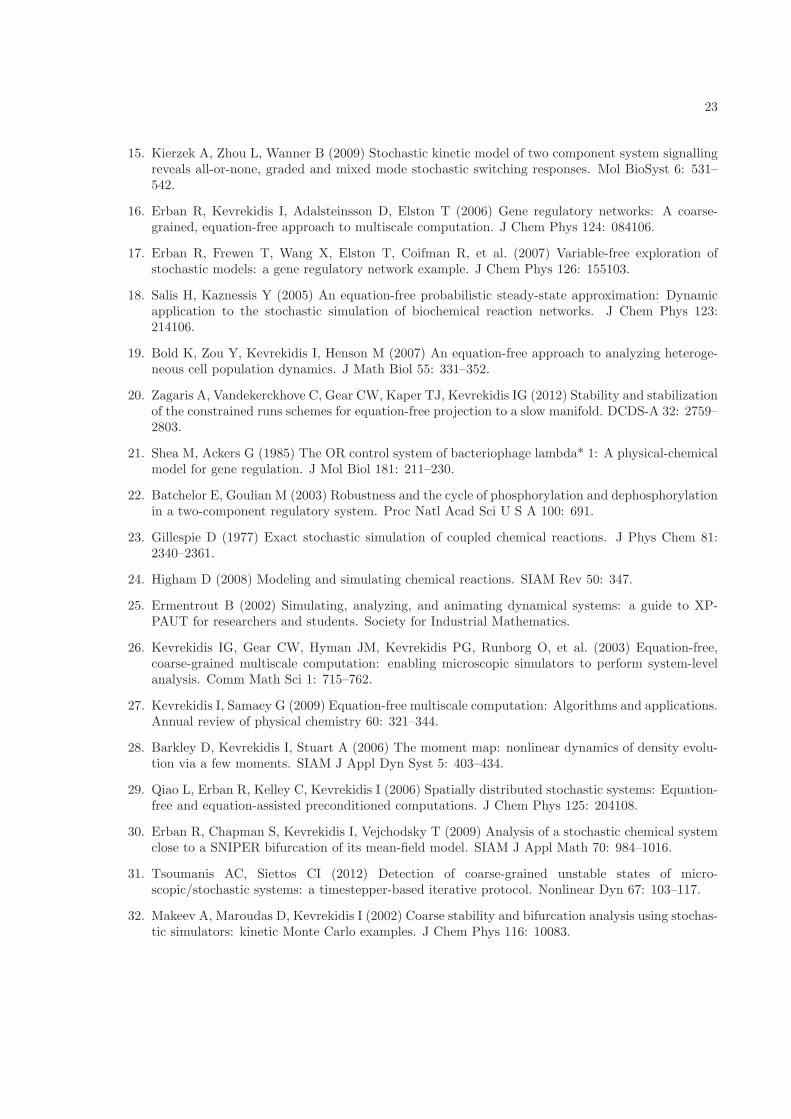
23

15. Kierzek A, Zhou L, Wanner B (2009) Stochastic kinetic model of two component system signallingreveals all-or-none, graded and mixed mode stochastic switching responses. Mol BioSyst 6: 531–542.

16. Erban R, Kevrekidis I, Adalsteinsson D, Elston T (2006) Gene regulatory networks: A coarse-grained, equation-free approach to multiscale computation. J Chem Phys 124: 084106.

17. Erban R, Frewen T, Wang X, Elston T, Coifman R, et al. (2007) Variable-free exploration ofstochastic models: a gene regulatory network example. J Chem Phys 126: 155103.

18. Salis H, Kaznessis Y (2005) An equation-free probabilistic steady-state approximation: Dynamicapplication to the stochastic simulation of biochemical reaction networks. J Chem Phys 123:214106.

19. Bold K, Zou Y, Kevrekidis I, Henson M (2007) An equation-free approach to analyzing heteroge-neous cell population dynamics. J Math Biol 55: 331–352.

20. Zagaris A, Vandekerckhove C, Gear CW, Kaper TJ, Kevrekidis IG (2012) Stability and stabilizationof the constrained runs schemes for equation-free projection to a slow manifold. DCDS-A 32: 2759–2803.

21. Shea M, Ackers G (1985) The OR control system of bacteriophage lambda* 1: A physical-chemicalmodel for gene regulation. J Mol Biol 181: 211–230.

22. Batchelor E, Goulian M (2003) Robustness and the cycle of phosphorylation and dephosphorylationin a two-component regulatory system. Proc Natl Acad Sci U S A 100: 691.

23. Gillespie D (1977) Exact stochastic simulation of coupled chemical reactions. J Phys Chem 81:2340–2361.

24. Higham D (2008) Modeling and simulating chemical reactions. SIAM Rev 50: 347.

25. Ermentrout B (2002) Simulating, analyzing, and animating dynamical systems: a guide to XP-PAUT for researchers and students. Society for Industrial Mathematics.

26. Kevrekidis IG, Gear CW, Hyman JM, Kevrekidis PG, Runborg O, et al. (2003) Equation-free,coarse-grained multiscale computation: enabling microscopic simulators to perform system-levelanalysis. Comm Math Sci 1: 715–762.

27. Kevrekidis I, Samaey G (2009) Equation-free multiscale computation: Algorithms and applications.Annual review of physical chemistry 60: 321–344.

28. Barkley D, Kevrekidis I, Stuart A (2006) The moment map: nonlinear dynamics of density evolu-tion via a few moments. SIAM J Appl Dyn Syst 5: 403–434.

29. Qiao L, Erban R, Kelley C, Kevrekidis I (2006) Spatially distributed stochastic systems: Equation-free and equation-assisted preconditioned computations. J Chem Phys 125: 204108.

30. Erban R, Chapman S, Kevrekidis I, Vejchodsky T (2009) Analysis of a stochastic chemical systemclose to a SNIPER bifurcation of its mean-field model. SIAM J Appl Math 70: 984–1016.

31. Tsoumanis AC, Siettos CI (2012) Detection of coarse-grained unstable states of micro-scopic/stochastic systems: a timestepper-based iterative protocol. Nonlinear Dyn 67: 103–117.

32. Makeev A, Maroudas D, Kevrekidis I (2002) Coarse stability and bifurcation analysis using stochas-tic simulators: kinetic Monte Carlo examples. J Chem Phys 116: 10083.

24

33. Hoch J (2000) Two-component and phosphorelay signal transduction. Curr Opin Cell Biol 3:165–170.

34. Baek S, Li A, Sassetti C (2011) Metabolic regulation of mycobacterial growth and antibiotic sen-sitivity. PLoS Biol 9: e1001065.

35. Kasahara M, Nakata A, H S (1992) Molecular analysis of the Escherichia coli PhoP-PhoQ operon.J Bacteriol 174: 492–8.

36. Compan I, Touati D (1994) Anaerobic activation of arcA transcription in Escherichia coli: roles ofFnr and ArcA. Mol Microbiol 11: 955–64.

37. Cai S, Inouye M (2002) EnvZ-OmpR interaction and osmoregulation in Escherichia coli. J BiolChem 277: 24155–61.

38. Cao Y, Gillespie D, Petzold L (2005) Avoiding negative populations in explicit Poisson tau-leaping.J Chem Phys 123: 054104.

25Table 1. Chemical reactions in the PhoBR E. coli stochastic kinetic model [15]

Description Reaction Propensity function Stochastic rate constant (s−1)

Activated transcription of RR RNAP + RR2P → mRNA-RR c1K2α0x11

1+K2α0x11+K1α0+K3x11c1 = 0.0751K1 = 9.23×106 Lmol−1

K2 = 6.76 × 1015 L2mol−2

K3 = 9.23× 106 Lmol−1

Basal transcription of RR RNAP → mRNA-RR c2K1α0

1+K2α0x11+K1α0+K3x11c2 = 10−4

Translation of RR mRNA-RR → RR+mRNA-RR c3X2 c3 = 0.1Degradation of RR mRNA mRNA-RR → d-mRNA-RR c4X2 c4 = 0.004Degradation of RR and variants RR,RRP,RR2P → d-RR c5X3, c5X1, c5X11 c5 = 6.42× 10−5

Transcription of HK prom-HK → mRNA-HK + prom-HK c6 c6 = 10−4

Translation of HK mRNA-HK → HK+mRNA-HK c7X10 c7 = 0.3Degradation of HK mRNA mRNA-HK → d-mRNA-HK c8X10 c8 = 0.004Degradation of HK and variants HK,HK2,HK2P → d-HK c9X4, c9X12, c9X5 c9 = 6.42× 10−5

Binding of RR to phosphorylated HK RR+HK2P → RR-HK2P c10X3X5 c10 = 10−4

Phosphorylation of RR RR-HK2P → HK2 + RRP c11X6 c11 = 1.6Binding of unphosphorylated RR to HK RRP +HK2 → RRP-HK2 c12X1X12 c12 = 10−4

Dephosphorylation of RR RRP-HK2 → RR+HK2 c13X7 c13 = 1.6Autophosphorylation of HK HK2 → HK2P c14X12 c14 = 0.05Dephosphorylation of HK HK2P → HK2 c15X5 c15 = 50.0 (varies)Activated transcription of reporter gene RNAP + RRP2 → mRNA-Rep c16K2α0x11

1+K2α0x11+K1α0+K3x11c16 = 0.3

Basal transcription of reporter gene RNAP → mRNA-Rep c17K1α0

1+K2α0x11+K1α0+K3x11c17 = 0.01

Translation of reporter gene mRNA-Rep → Rep +mRNA-Rep c18X8 c18 = 0.1Degradation of reporter transcript mRNA-Rep → d-mRNA-Rep c19X8 c19 = 0.004Degradation of reporter Rep → d-Rep c20X9 c20 = 6.42× 10−5

Dissociation of HK dimer HK2 → 2HK c21X12 c21 = 0.5Association of HK dimer 2HK → HK2 c22X4(X4 − 1) c22 = 0.1Dissociation of phosphorylated RR dimer RR2P → 2RRP c23X11 c23 = 0.5Association of phosphorylated RR dimer 2RRP → RR2P c24X1(X1 − 1) c24 = 8.3× 10−2

Reactions included in the KZW stochastic model [15], together with the associated propensity functions and values of the stochastic rateconstants. Values given are for the autoregulated, slow transcription case. The value of c15 varies with the external signal in oursimulations. d-mRNA-RR, d-RR, d-mRNA-HK, d-HK, d-mRNA-Rep and d-Rep are degradation products of mRNA-RR, RR,mRNA-HK, HK, mRNA-Rep and Rep respectively. prom-HK is the promoter region of the HK gene.

26

Table 2. Correspondence between chemical species and model variables

Chemical species Short name Concentration Number of molecules

Phosphorylated response regulator protein RRP x1 X1

mRNA of response regulator mRNA-RR x2 X2

Response regulator protein RR x3 X3

Histidine kinase protein HK x4 X4

Phosphorylated histidine kinase dimer HK2P x5 X5

Complex of RR and phosphorylated HK dimer RR-HK2P x6 X6

Complex of phosphorylated RR and HK dimer RRP-HK2 x7 X7

mRNA of reporter mRNA-Rep x8 X8

Reporter protein Rep x9 X9

mRNA of histidine kinase mRNA-HK x10 X10

Phosphorylated response regulator dimer RR2P x11 X11

Histidine kinase dimer HK2 x12 X12

27

reporter gene

reporter mRNA reporter

RR gene HK gene

RR mRNA HK mRNA

RRp RR

P

P

HKp HK

Figure 1. Simplified diagram of the KZW stochastic TCS model. (After [15].)

28

1.0

0.0

0.5

0.01

0.1

10

0.01

0.1

10

0.0001

0.001

10

0.0001

0.001

10

a

b

c

d

Number of reporter protein molecules

0 30,000 15,000

Sig

nal s

trength

Figure 2. Results of Kierzek, Zhou and Wanner [15]. Histograms of 10,000 realisations at timet = 20, 000s, as fractions of largest value: for a) autoregulated RR gene & fast transcription of HK; b)autoregulated RR gene & slow transcription of HK; c) constitutively expressed RR gene & fasttranscription of HK; d) constitutively expressed RR gene & slow transcription of HK. (Adaptedfrom [15]. Reproduced by permission of The Royal Society of Chemistry.)

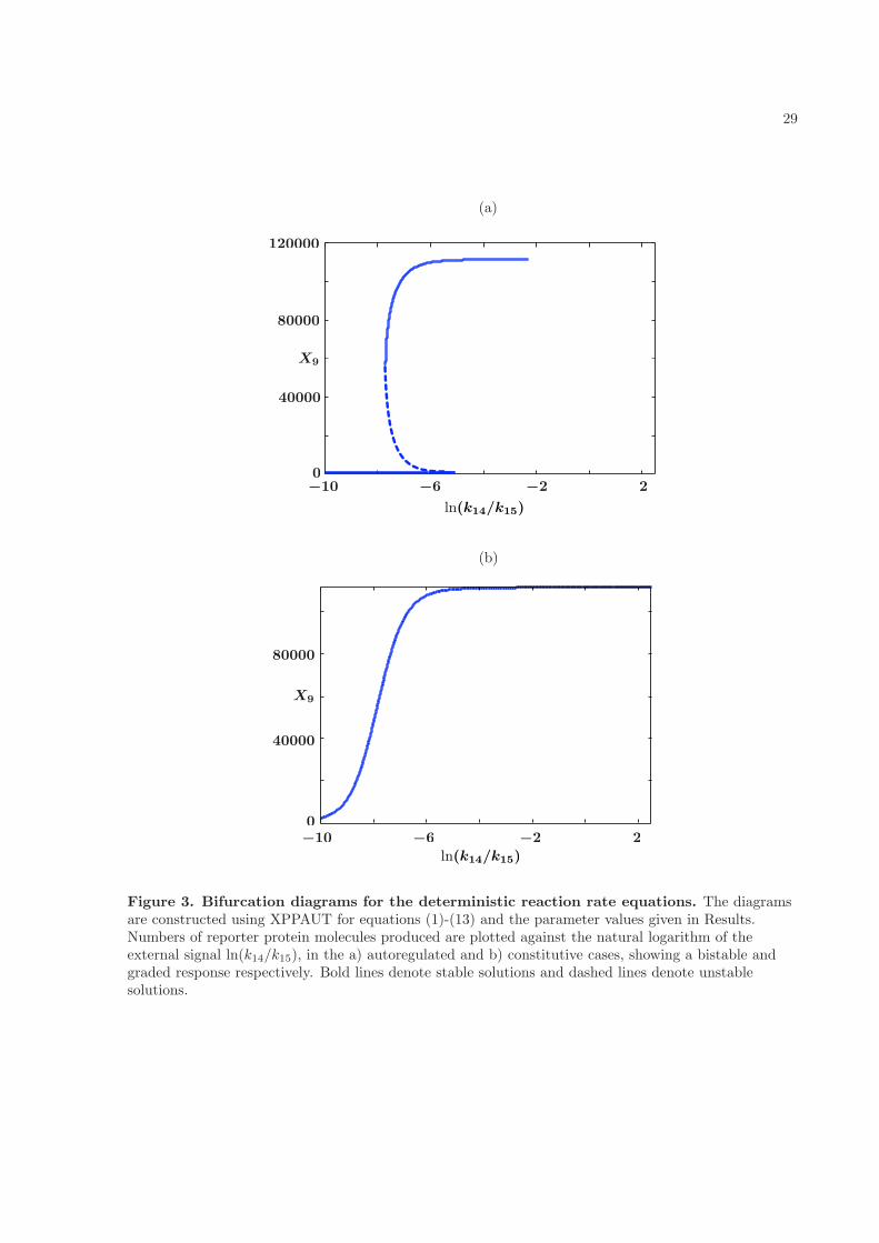
29

−10 −6 −2 2

0

40000

80000

X9

X9

−10 −6 −2 2

0

40000

80000

120000

(a)

(b)

ln(k14/k15)

ln(k14/k15)

Figure 3. Bifurcation diagrams for the deterministic reaction rate equations. The diagramsare constructed using XPPAUT for equations (1)-(13) and the parameter values given in Results.Numbers of reporter protein molecules produced are plotted against the natural logarithm of theexternal signal ln(k14/k15), in the a) autoregulated and b) constitutive cases, showing a bistable andgraded response respectively. Bold lines denote stable solutions and dashed lines denote unstablesolutions.

30

Figure 4. Timescales of persistence for approximate basal solution. Steady states are shownfor the mean number of phosphorylated RR dimer molecules, Y11, in equation (70), found using theequation-free numerical approach and poor man’s continuation, starting from the lowest value of theexternal signal and an approximate basal solution or a zero solution and continuing towards highersignal values. The mean number of molecules produced is plotted against the natural logarithm of theexternal signal ln(c14/c15) in the a) autoregulated fast transcription (th = 300s and 500s), b)autoregulated slow transcription (th = 300s and 500s), c) constitutively expressed fast transcription(th = 30s and 50s) and d) constitutively expressed slow transcription (th = 300s and 500s) cases. Wherethe two curves coincide, the th = 500s points are plotted and the th = 300s points are underlying.

31

Figure 5. Stability of basal solutions. Spectrum of the Jacobian of the coarse time-stepper Φth

evaluated at basal solutions with low and high external signals for a) autoregulated fast transcription(th = 500s), b) autoregulated slow transcription (th = 500s), c) constitutively expressed fasttranscription (th = 50s) and d) constitutively expressed slow transcription (th = 500s) cases.Eigenvalues outside the unit circle (plotted in blue) indicate that the corresponding steady state isunstable. Eigenvalues corresponding to a spectrum that is stable overall are plotted as red circles.Eigenvalues corresponding to a spectrum that is unstable overall are plotted as green asterisks. In a),b), d) and the upper panel of c) one instance of the spectrum (of the 10 calculated) is shown. In thelower panel of c) two instances of the spectrum (of the 20 calculated) are shown: one stable and oneunstable example.

32

Figure 6. Equation-free tracking of induced expression states. Steady states are shown for themean number of phosphorylated RR dimer molecules, Y11, in equation (70), found using theequation-free numerical approach and poor man’s continuation, starting from the highest value of theexternal signal and a point in the vicinity of the deterministic reaction rate solution and continuingtowards lower signal values. The mean number of molecules produced is plotted against the naturallogarithm of the external signal ln(c14/c15) for time horizon th = 200s in the a) autoregulated fasttranscription, b) autoregulated slow transcription, c) constitutively expressed fast transcription and d)constitutively expressed slow transcription cases. Spectra of stable steady states at the highest value ofthe external signal are plotted in the insets.

33

Figure 7. Graded response in the constitutively expressed fast transcription case. Theequation-free tracking of the induced state in the constitutively expressed fast transcription case showsa graded response for th = 100s in one run. This behaviour is lost upon increasing the time horizon toth = 200s (see also Fig. 6c).