190

EPILYSIS, a New Solver for Finite Element Analysis

George Korbetis, Serafim Chatzimoisiadis, Dimitrios Drougkas, BETA CAE Systems,

Thessaloniki/Greece, ansa@beta-cae.com

Abstract

This paper introduces EPILYSIS, the new member of BETA CAE Systems software suite. EPILYSIS is

a solver for Finite Element Analysis, which comes to bridge the gap between pre- and post-

processing and offer a seamless operation in CAE workflow. Designed for large-scale model

analyses, it is ideal for the global strength assessment of large vessels and detailed strength

assessment of highly stressed areas. Additionally, direct and modal frequency response and non-

linear contact solutions allow more extensive and sophisticated analyses. EPILYSIS together with the

pre- and post- processors, ANSA and META, offer a valuable yet affordable tool to the Marine

Engineering sector. Two characteristic case studies are presented where EPILYSIS element accuracy

and results performance are compared with well-known solvers in the market.

1. Introduction

EPILYSIS is the new addition to the BETA CAE Systems analysis tools. Named after the Greek word

for "solution", EPILYSIS covers numerous solution types such as Structural, NVH, Optimization and

more. In this paper, two representative applications are presented, where the complete BETA CAE

Systems suite is used for the model preparation, process and results interpretation.

In the first part, a typical VLCC vessel is subjected to three different loading conditions. The main

target is the determination of the maximum stresses and the critical areas. The complete Model set-up

is conducted with the aid of the ANSA pre-processor. First, a detailed Finite Element model of the

hull structure is generated, complying with the meshing requirements set by Classification Societies.

Then, a series of useful and automated processes make the model "lighter", more sophisticated but

still realistic and suitable for the strength analysis. For each loading condition, the hydrostatic

equilibrium of the ship is computed and the corresponding hull deformations are calculated. The static

analyses are conducted using both the EPILYSIS and a well-known commercial solver.

In the second part, EPILYSIS solver is used on a nonlinear-contact strength analysis for a ship’s

rudder. The applied force which is produced by the water resistance, at specific speed and angle-

position of the rudder, is calculated by a simplified CFD analysis and used as the loading condition

for the structural analysis. The static problem set-up is performed using automated processes, such as

the results mapping, the contact pair definition and the batch meshing, which are provided by the

ANSA pre-processor. Several runs are performed with EPILYSIS and an industry standard solver.

The solvers are compared to each other concerning the performance and the results accuracy.

2. Static Analysis

2.1. Model set-up

The general characteristics of the studied VLCC are presented in Table I. At first, a Finite Element

(FE) model of the ship structure is automatically generated. In general, the ship is relatively large so,

coarse mesh should be applied to avoid very long simulation time. The whole structure is represented

by first-order shell elements; (a small amount of solid tetrahedral elements are used at the stern tube

region). A coarse mesh is generated for the whole structure (element length of 0.95 m), except from

selected areas, where finer mesh (e.g. 0.2 m) ensures better results accuracy. This mesh strategy was

selected to contribute to the solvers comparison.

191

Table I: Main characteristics of the VLCC vessel of the present study

Type Crude Oil Tanker

Deadweight 320000 t

Length betw. Perp. LPP 320.00 m

Breadth B 60.00 m

Depth D 30.50 m

Scantling draft T 22.50 m

Service speed Vs 15.9 kn

Main engine Wärtsilä 7RT-FLEX84T-D

Keel laid April 2010

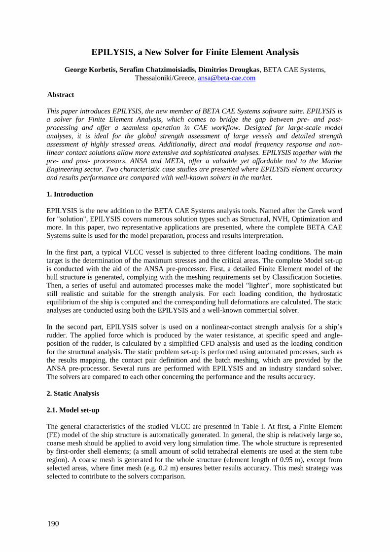
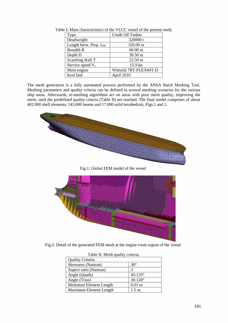
The mesh generation is a fully automated process performed by the ANSA Batch Meshing Tool.

Meshing parameters and quality criteria can be defined in several meshing scenarios for the various

ship areas. Afterwards, re-meshing algorithms act on areas with poor mesh quality, improving the

mesh, until the predefined quality criteria (Table II) are reached. The final model comprises of about

402.000 shell elements, 143.000 beams and 17.000 solid tetrahedrals, Figs.1 and 2.

Fig.1: Global FEM model of the vessel

Fig.2: Detail of the generated FEM mesh at the engine room region of the vessel

Table II: Mesh quality criteria.

Quality Criteria

Skewness (Nastran) 30°

Aspect ratio (Nastran) 3

Angle (Quads) 45-135°

Angle (Trias) 30-120°

Minimum Element Length 0.01 m

Maximum Element Length 1.5 m

192

In addition, geometrical simplifications should be applied on the model. The first action to simplify

the model is to fill small holes that are not significant for the model’s behavior. Such holes are

automatically identified according to their diameter and filled. This action improves the element

quality while reduces the number of elements. This process is prescribed at the meshing parameters of

the Batch Meshing Scenario. Thus, the whole process runs in batch mode without any need of user

interaction. The second simplification is the replacement of longitudinal stiffeners by beam elements.

This method simplifies the model by avoiding the generation of very small shell elements. The

properties of the beam elements are auto-calculated in accordance with the cross section of each

stiffener.

Machinery, auxiliary structures and small constructions that do not contribute to ship’s strength are

not modeled in the present FE model. Their mass is applied to the model as non-structural mass. This

mass is appropriately distributed over the FE model, so as to reach the prescribed lightship weight and

the corresponding center of gravity. The mass of the present structural model is 34442 t, while the

lightship weight is 43938.7 t and its center of gravity L.C.G. at 151.338 m. Thus, 9496.7 t of lumped

masses are appropriately distributed in holds, stern and bow by the automatic process of the ANSA

Mass Balance Tool, Fig.3. Finally, the engine mass is represented by a lumped mass of 990 t

distributed to the engine foundation positions by Rigid Body Elements (RBE3-distributing) elements.

Fig.3: Distribution of non-structural mass in the present FEM model

Ballast arrival (L.C. 1)

Displacement: 145647 t

Draft: 9.69 m

Trim: 2.12 m

Full-load departure (L.C. 2)

Displacement: 364074 t

Draft: 22.52 m

Trim: 0.11 m

Departure, partial load (L.C. 3)

Displacement: 229276 t

Draft: 14.78 m

Trim: 3.05 m

Fig.4: Representative loading conditions of the vessel

Fig.5: Application of hydrostatic pressure due to buoyancy in the FEM model

168 tons

1360 tons

532 tons 208 tons

1334 tons 1205 tons

24 tons

911 tons

130 tons 167 tons

179 tons

358 tons 1918 tons

193

Three representative loading conditions (full-load departure, ballast arrival and departure with partial

load) are considered in the present analysis, Fig.4. The contents of the tanks are represented by

lumped mass connected to each hold bottom with RBE3 elements. The ship is positioned on still

water considering the vessel’s total displacement and center of gravity. Buoyancy is applied as

pressure at the hull underneath the waterline using Pressure Load (PLOAD4) entities, Fig.5. Finally,

the vessel is trimmed in order to achieve static equilibrium between weight and buoyancy.

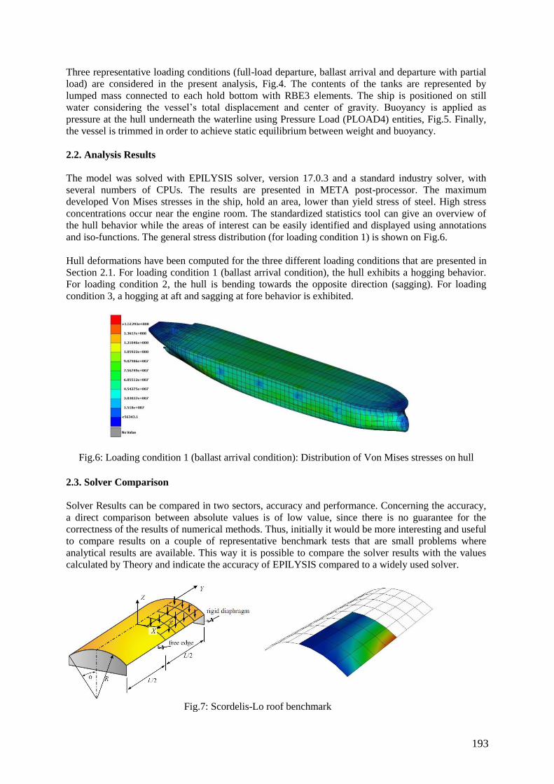
2.2. Analysis Results

The model was solved with EPILYSIS solver, version 17.0.3 and a standard industry solver, with

several numbers of CPUs. The results are presented in META post-processor. The maximum

developed Von Mises stresses in the ship, hold an area, lower than yield stress of steel. High stress

concentrations occur near the engine room. The standardized statistics tool can give an overview of

the hull behavior while the areas of interest can be easily identified and displayed using annotations

and iso-functions. The general stress distribution (for loading condition 1) is shown on Fig.6.

Hull deformations have been computed for the three different loading conditions that are presented in

Section 2.1. For loading condition 1 (ballast arrival condition), the hull exhibits a hogging behavior.

For loading condition 2, the hull is bending towards the opposite direction (sagging). For loading

condition 3, a hogging at aft and sagging at fore behavior is exhibited.

Fig.6: Loading condition 1 (ballast arrival condition): Distribution of Von Mises stresses on hull

2.3. Solver Comparison

Solver Results can be compared in two sectors, accuracy and performance. Concerning the accuracy,

a direct comparison between absolute values is of low value, since there is no guarantee for the

correctness of the results of numerical methods. Thus, initially it would be more interesting and useful

to compare results on a couple of representative benchmark tests that are small problems where

analytical results are available. This way it is possible to compare the solver results with the values

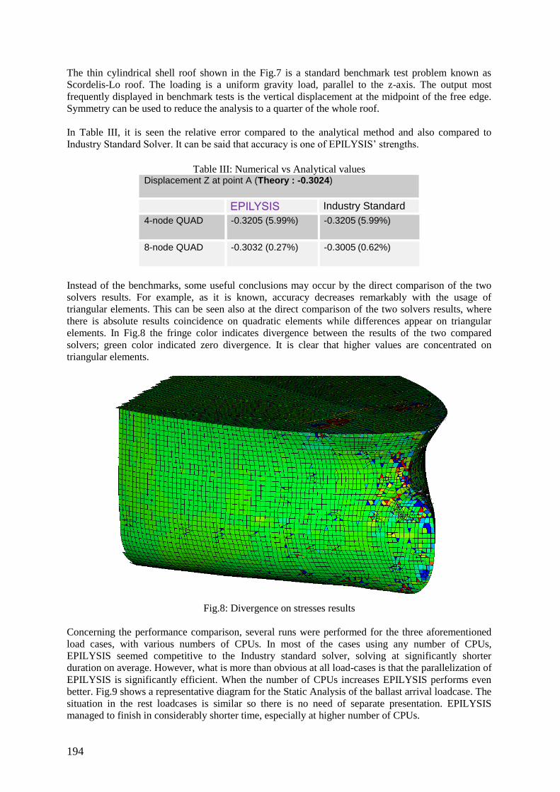
calculated by Theory and indicate the accuracy of EPILYSIS compared to a widely used solver.

Fig.7: Scordelis-Lo roof benchmark

194

The thin cylindrical shell roof shown in the Fig.7 is a standard benchmark test problem known as

Scordelis-Lo roof. The loading is a uniform gravity load, parallel to the z-axis. The output most

frequently displayed in benchmark tests is the vertical displacement at the midpoint of the free edge.

Symmetry can be used to reduce the analysis to a quarter of the whole roof.

In Table III, it is seen the relative error compared to the analytical method and also compared to

Industry Standard Solver. It can be said that accuracy is one of EPILYSIS’ strengths.

Table III: Numerical vs Analytical values

Displacement Z at point A (Theory : -0.3024)

EPILYSIS Industry Standard

4-node QUAD -0.3205 (5.99%) -0.3205 (5.99%)

8-node QUAD -0.3032 (0.27%) -0.3005 (0.62%)

Instead of the benchmarks, some useful conclusions may occur by the direct comparison of the two

solvers results. For example, as it is known, accuracy decreases remarkably with the usage of

triangular elements. This can be seen also at the direct comparison of the two solvers results, where

there is absolute results coincidence on quadratic elements while differences appear on triangular

elements. In Fig.8 the fringe color indicates divergence between the results of the two compared

solvers; green color indicated zero divergence. It is clear that higher values are concentrated on

triangular elements.

Fig.8: Divergence on stresses results

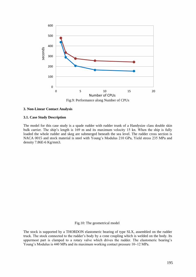
Concerning the performance comparison, several runs were performed for the three aforementioned

load cases, with various numbers of CPUs. In most of the cases using any number of CPUs,

EPILYSIS seemed competitive to the Industry standard solver, solving at significantly shorter

duration on average. However, what is more than obvious at all load-cases is that the parallelization of

EPILYSIS is significantly efficient. When the number of CPUs increases EPILYSIS performs even

better. Fig.9 shows a representative diagram for the Static Analysis of the ballast arrival loadcase. The

situation in the rest loadcases is similar so there is no need of separate presentation. EPILYSIS

managed to finish in considerably shorter time, especially at higher number of CPUs.

195

Fig.9: Performance along Number of CPUs

3. Non-Linear Contact Analysis

3.1. Case Study Description

The model for this case study is a spade rudder with rudder trunk of a Handysize class double skin

bulk carrier. The ship’s length is 169 m and its maximum velocity 15 kn. When the ship is fully

loaded the whole rudder and skeg are submerged beneath the sea level. The rudder cross section is

NACA 0015 and stock material is steel with Young’s Modulus 210 GPa, Yield stress 235 MPa and

density 7.86E-6 Kg/mm3.

Fig.10: The geometrical model

The stock is supported by a THORDON elastomeric bearing of type SLX, assembled on the rudder

truck. The stock connected to the rudder’s body by a cone coupling which is welded on the body. Its

uppermost part is clamped to a rotary valve which drives the rudder. The elastomeric bearing’s

Young’s Modulus is 440 MPa and its maximum working contact pressure 10~12 MPa.

0 5 10 15 20

0

100

200

300

400

500

600

Number of CPUs

seco

nd

sStandart Solver

EPILYSIS 17.0.3.

196

The main force that strains the rudder is produced by the water flow around it. As expected, the

maximum force appears at the vessel’s full speed, when the rudder turns to the maximum angle of 35

degrees. The weight and buoyancy are considerably small in relation to the water flow force therefore

they are not taken into account. To evaluate the force that is distributed to the whole surface of the

rudder, a CFD analysis is performed for the described extreme conditions. This analysis is performed

in ANSYS FLUENT. The results from the CFD analysis are mapped to the structural model and used

as boundary conditions to the structural analysis. The geometrical model is shown in Fig.10.

To complete the FE model that will be exported to the solver, the proper materials, shell and solid

element properties, and the solver header are defined. Solver output requests are defined for strain and

stress.

3.2. Model Set-up

This structural analysis aims to calculate the strength of the rudder assembly and stresses on the

contact between the bearing and the stock. The FE representation of the geometrical model that

participates in the analysis is shown in Fig.11.

y

Fig.10: The rudder body & skeg mesh

The rudder stock and the bearing are important parts for this analysis and their results need to be

accurate. Thus, thin layers of Hexahedral solid (HEXA) elements are applied on the stock perimeter to

ensure the accuracy of the desired results. In addition, the whole stock model is meshed with HEXA

elements. The HEXA meshing process is a semi-automatic process in ANSA based on special entities,

the Hexa Boxes that are fit on the model. Boxes are re-usable and have their own meshing parameters

such as, node number, spacing and number of layers etc. After the definition of the Hexa Boxes, mesh

is created automatically. Three layers of HEXA elements are applied on the stock / bearing contact

area with small element length of 4.5 mm, while the rest of the part is meshed with 30 mm HEXA

elements. The bearing is also meshed with HEXA elements.

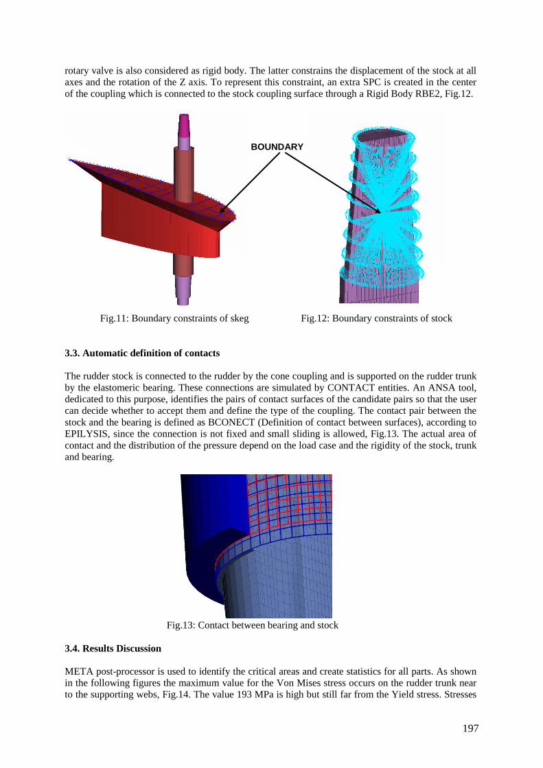
The structural analysis is limited to the rudder assembly, so the rest of the ship is considered as rigid.

Thus, boundary conditions [Single Point Constraints-SPC] are applied on the upper nodes of the

rudder skeg which constrain the displacement and rotation in all degrees of freedom, Fig.11. The

197

rotary valve is also considered as rigid body. The latter constrains the displacement of the stock at all

axes and the rotation of the Z axis. To represent this constraint, an extra SPC is created in the center

of the coupling which is connected to the stock coupling surface through a Rigid Body RBE2, Fig.12.

Fig.11: Boundary constraints of skeg Fig.12: Boundary constraints of stock

3.3. Automatic definition of contacts

The rudder stock is connected to the rudder by the cone coupling and is supported on the rudder trunk

by the elastomeric bearing. These connections are simulated by CONTACT entities. An ANSA tool,

dedicated to this purpose, identifies the pairs of contact surfaces of the candidate pairs so that the user

can decide whether to accept them and define the type of the coupling. The contact pair between the

stock and the bearing is defined as BCONECT (Definition of contact between surfaces), according to

EPILYSIS, since the connection is not fixed and small sliding is allowed, Fig.13. The actual area of

contact and the distribution of the pressure depend on the load case and the rigidity of the stock, trunk

and bearing.

Fig.13: Contact between bearing and stock

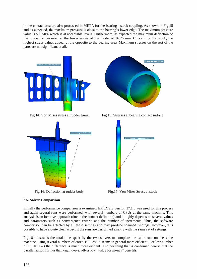
3.4. Results Discussion

META post-processor is used to identify the critical areas and create statistics for all parts. As shown

in the following figures the maximum value for the Von Mises stress occurs on the rudder trunk near

to the supporting webs, Fig.14. The value 193 MPa is high but still far from the Yield stress. Stresses

BOUNDARY

198

in the contact area are also processed in META for the bearing - stock coupling. As shown in Fig.15

and as expected, the maximum pressure is close to the bearing’s lower edge. The maximum pressure

value is 5.1 MPa which is at acceptable levels. Furthermore, as expected the maximum deflection of

the rudder is measured at the lower nodes of the model at 36.26 mm. Concerning the Stock, the

highest stress values appear at the opposite to the bearing area. Maximum stresses on the rest of the

parts are not significant at all.

Fig.14: Von Mises stress at rudder trunk Fig.15: Stresses at bearing contact surface

Fig.16: Deflection at rudder body Fig.17: Von Mises Stress at stock

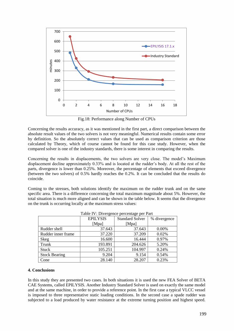
3.5. Solver Comparison

Initially the performance comparison is examined. EPILYSIS version 17.1.0 was used for this process

and again several runs were performed, with several numbers of CPUs at the same machine. This

analysis is an iterative approach (due to the contact definition) and it highly depends on several values

and parameters such as convergence criteria and the number of increments. Thus, the software

comparison can be affected by all these settings and may produce spanned findings. However, it is

possible to have a quite clear aspect if the runs are performed exactly with the same set of settings.

Fig.18 illustrates the total time spent by the two solvers to complete the same run, on the same

machine, using several numbers of cores. EPILYSIS seems in general more efficient. For low number

of CPUs (1-2) the difference is much more evident. Another thing that is confirmed here is that the

parallelization further than eight cores, offers low “value for money” benefits.

199

Fig.18: Performance along Number of CPUs

Concerning the results accuracy, as it was mentioned in the first part, a direct comparison between the

absolute result values of the two solvers is not very meaningful. Numerical results contain some error

by definition. So the absolutely correct values that can be used as comparison criterion are those

calculated by Theory, which of course cannot be found for this case study. However, when the

compared solver is one of the industry standards, there is some interest in comparing the results.

Concerning the results in displacements, the two solvers are very close. The model’s Maximum

displacement decline approximately 0.33% and is located at the rudder’s body. At all the rest of the

parts, divergence is lower than 0.25%. Moreover, the percentage of elements that exceed divergence

(between the two solvers) of 0.5% hardly reaches the 0.2%. It can be concluded that the results do

coincide.

Coming to the stresses, both solutions identify the maximum on the rudder trunk and on the same

specific area. There is a difference concerning the total maximum magnitude about 5%. However, the

total situation is much more aligned and can be shown in the table below. It seems that the divergence

on the trunk is occurring locally at the maximum stress values:

Table IV: Divergence percentage per Part

EPILYSIS

[Mpa]

Standard Solver

[Mpa]

% divergence

Rudder shell 37.643 37.643 0.00%

Rudder inner frame 37.220 37.209 0.02%

Skeg 16.600 16.444 0.97%

Trunk 193.891 204.626 5.20%

Stuck 105.251 104.997 0.24%

Stock Bearing 9.204 9.154 0.54%

Cone 28.140 28.207 0.23%

4. Conclusions

In this study they are presented two cases. In both situations it is used the new FEA Solver of BETA

CAE Systems, called EPILYSIS. Another Industry Standard Solver is used on exactly the same model

and at the same machine, in order to provide a reference point. In the first case a typical VLCC vessel

is imposed to three representative static loading conditions. In the second case a spade rudder was

subjected to a load produced by water resistance at the extreme turning position and highest speed.

0

100

200

300

400

500

600

700

0 2 4 6 8 10 12 14 16 18

min

ute

s

Number of CPUs

EPILYSIS 17.1.x

Industry Standard

200

What makes this analysis more special is the contact definition between the rudder stuck and a

bearing made of Thordon material. For the analysis set up of such big and detailed models the use of

sophisticated tools that automate and facilitate the simulation process (like Batch Meshing, Results

Mapper and Contact Wizard) turns to be a matter of great importance. ANSA and μETA pre- and

post- processors have been used successfully for the definition of CFD and structural analysis.

Analysis results, generated by the two solvers, referring mainly to the Stresses and Deformations, are

presented and analyzed by META post-processor and compared to each other. In terms of

Deformation there is absolute coincidence between the two Solvers. The stress results are also more

or less aligned for Quadratic elements while for Triangular elements there is much higher divergence.

It is also presented a performance comparison between the two Solvers, for both case studies. Even

though in the second case the performance strongly depends on the analyses’ characteristic values like

convergence criteria, mesh density, material characteristic values etc., in general it seems that

EPILYSIS solver reaches quite high performance standards for any number of CPUs. Additionally,

the parallelization of EPILYSIS seems quite more efficient especially in the first Linear Static case

study.

References

DAHLER G.; BRODIN, E.; VARTDAL, B.J.; CHISTENSEN, H.W.; JAKOBSEN, S.B.; OK, Y.K.;

HEO, J.H.; PARK, K.R. (2004), A study on flexible hulls, flexible engines, crank shaft deflections and

engine bearing loads for VLCC propulsion machinery, CIMAC Congress, Kyoto

DEVANNEY, J.; KENNEDY, M. (2003), The down ratchet and the deterioration of tanker new-

building standards, Center for Tankship Excellence

RAWSON, K.J.; TUPPER, E.C. (1997), Basic Ship Theory, Elsevier, pp.555-563

GL RULES and GUIDELINES (2011), Rudder and Manoeuvring Arrangement, Germanischer Lloyd,

Hamburg

GL RULES and GUIDELINES (2011), Steel Plates, Strips, Sections and Bars, Germanischer Lloyd,

Hamburg