Eur. Phys. J. B (2018) 91: 267https://doi.org/10.1140/epjb/e2018-90136-3 THE EUROPEAN

PHYSICAL JOURNAL BRegular Article

Epidemiological impact of waning immunization on a vaccinatedpopulationEwa Grela, Michael Sticha, and Amit K Chattopadhyay

Mathematics, Systems Analytics Research Institute, School of Engineering and Applied Science, Aston University,Aston Triangle, Birmingham B4 7ET, UK

Received 6 March 2018 / Received in final form 14 June 2018Published online 1 November 2018c© The Author(s) 2018. This article is published with open access at Springerlink.com

Abstract. This is an epidemiological SIRV model based study that is designed to analyze the impact ofvaccination in containing infection spread, in a 4-tiered population compartment comprised of suscepti-ble, infected, recovered and vaccinated agents. While many models assume a lifelong protection throughvaccination, we focus on the impact of waning immunization due to conversion of vaccinated and recov-ered agents back to susceptible ones. Two asymptotic states exist, the “disease-free equilibrium” and the“endemic equilibrium” and we express the transitions between these states as function of the vaccinationand conversion rates and using the basic reproduction number. We find that the vaccination of newbornsand adults have different consequences on controlling an epidemic. Also, a decaying disease protectionwithin the recovered sub-population is not sufficient to trigger an epidemic at the linear level. We performsimulations for a parameter set mimicking a disease with waning immunization like pertussis. For a diffu-sively coupled population, a transition to the endemic state can proceed via the propagation of a travelinginfection wave, described successfully within a Fisher-Kolmogorov framework.

1 Introduction

Infectious diseases have a strong impact on the dynam-ics of human populations and are routinely highlightedwhen epidemic outbreaks of deadly infections like Ebolaor MERS occur. Increased human mobility, the rise ofpathogens resistant to antibiotics (“Antimicrobial Resis-tance”), and the advent of new, so called EmergingInfectious Diseases are making infectious diseases a majorhealth challenge of the 21st century.

To understand more deeply transmitting diseases andepidemic outbreaks and to inform public health organi-zations, a wide range of mathematical models have beenproposed and studied in detail. One of the simplest andwell-known models illustrating the dynamics of epidemicsis the SIR model, proposed by Kermack and McKendrickin 1927 [1]. The central idea of this model is to dividethe entire population into three separate groups: suscep-tible (S) individuals that have never been infected andare not immune to the disease; infected (I) individuals,who are infectious and can spread the disease within thepopulation; and recovered (or removed; R) individuals whohave already had the disease and are therefore immune forlife.

a e-mail: m.stich@aston.ac.uk

Temporal changes in the numbers of individuals in dif-ferent groups of the SIR model are described by thedifferential equations

dS

dt= −βSI, (1a)

dI

dt= βSI − aI, (1b)

dR

dt= aI. (1c)

The number of infected agents increases proportionallywith the number of susceptible agents times the force ofinfection βI, being itself the product of the non-zero infec-tion rate β and the number of infectious individuals. Thisis an example of a density dependent force of infection,being an alternative a frequency dependent force of infec-tion βI/N [2]. Individuals recover from the infection withrate a.

Adding equations (1a)–(1c), one can see that S + I +Ris time conserved. Furthermore, there is no notion ofphysical space in the model, meaning that individualsare uniformly mixed in the population. Both propertiesare common assumptions of simple SIR models that arerarely realized in real populations.

Page 2 of 11 Eur. Phys. J. B (2018) 91: 267

One of the key medical advances of the 20th century wasthe proliferation of cheap and safe vaccines for a range ofdiseases. Vaccines are among the most important tools toprevent infections and epidemics. One particular benefi-cial and mathematically interesting aspect of vaccinationis that not 100% of a population need to be immunized inorder to prevent epidemic outbreaks, a property calledherd immunity [2]. Unfortunately, vaccination encoun-ters opposition in different socio-cultural contexts thatendangers the working of the herd immunity effect as thefraction of vaccinated individuals falls below a threshold.Yet another effect that limits the efficiency of vaccines isthat the protection provided has a finite lifetime: depend-ing on the disease, the immunization effect of the vaccinefades over time and the patient has to be re-vaccinated(e.g., diphtheria, tetanus and pertussis).

In this article, we investigate an SIRV model (“V” forvaccination) that accounts for the fact that immunizationof the vaccine wanes over time and that even recoveredindividuals can fall ill again. Furthermore, we consider thespatiotemporal dynamics of such a system. Epidemiologi-cal and SIRV models have been considered in many vari-ants, for reviews see references [2–4], and some recent workconsider the dynamics on networks [5–7], information-driven vaccination [8–10], or stochastic behavior [11,12].Spatiotemporal dynamics in nonlinear systems often showtraveling wave patterns or Turing-like, stationary pat-terns [13,14]. In the context of spatial epidemiologi-cal models [15], spatial coupling is often described byreaction-diffusion equations or networks [16–22].

2 The SIRV model with finite lifetimeprotection

Among the range of epidemiological models using the SIRmodel as a building block, we focus on those aimed toinvestigate the impact of vaccination, using here a modi-fication of the SIRV models presented in references [4,23].In this model, an independent birth rate B and deathrate p are taken into account. There are two types of vac-cination: v1 is the fraction of vaccinated newborns and v2is the rate of vaccination of susceptible individuals. Byconstruction, 0 ≤ v1 ≤ 1, with these two limiting casesrepresenting that all newborns are either susceptible orvaccinated. Contrary to the classical SIR model, protec-tion against infection is not for life: recovered individualsbecome susceptible again with rate q1, vaccinated oneswith rate q2, yielding the model

dS

dt= B(1− v1)− βSI − v2S + q1R+ q2V − pS,(2a)

dI

dt= βSI − aI − pI, (2b)

dR

dt= aI − q1R− pR, (2c)

dV

dt= v1B + v2S − q2V − pV . (2d)

A schematic representation of the transitions among thecompartments in the SIRV model is displayed in Figure 1

Fig. 1. Schematic representation of the transition of individ-uals in the SIRV model (SIR model with additional effect ofvaccination) for infectious diseases.

Table 1. Parameters used in model (2). The parametersβ, a, p and B are positive, the others non-negative and 0 ≤v1 ≤ 1. All parameters are measured per unit time, exceptfor v1 (unitless) and β (per unit time times population sizeunit).

Parameter Description

β Infection ratea Recovery rate from infectionp Death rateB Birth ratev1 Fraction of vaccinated newbornsv2 Vaccination rate of susceptible individualsq1 Conversion rate from recovered to susceptibleq2 Conversion rate from vaccinated to susceptible

and the meaning of the parameters is found in Table 1.All parameters and variables have to be non-negative forequations (2) being interpreted as a valid epidemiologicalmodel.

From equations (2a)–(2d), and defining the total popu-lation size as N(t) = S + I +R+ V , we find

dN

dt= B − pN. (3)

This linear equation has the solution

N(t) =B

p+

(N0 −

B

p

)e−pt, (4)

where N0 is the initial population size. While the totalpopulation size can vary as a transient if N0 6= B/p, inthe limit lim

t→∞N = B/p which means that asymptotically

the total population size is constant. In particular, if birthand death rates are equal, then lim

t→∞N = 1. In the follow-

ing, we require both birth and death rates to be strictly

Eur. Phys. J. B (2018) 91: 267 Page 3 of 11

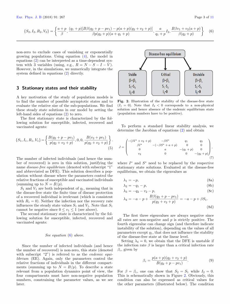
{S2, I2, R2, V2} =

{a+ p

β,

(q1 + p)[Bβ(q2 + p− pv1)− p(a+ p)(q2 + v2 + p)]

βp(q2 + p)(a+ q1 + p),

a

q1 + pI2,

Bβv1 + v2(a+ p)

β(q2 + p)

}(6)

non-zero to exclude cases of vanishing or exponentiallygrowing populations. Using equation (4), the model inequations (2) can be interpreted as a time-dependent sys-tem with 3 variables (using, e.g., R = N − S − I − V ).However, in the simulations, we numerically integrate thesystem defined in equations (2) directly.

3 Stationary states and their stability

A key motivation of the study of population models isto find the number of possible asymptotic states and toevaluate the relative size of the sub-populations. We findthese steady state solutions in our model by setting theleft-hand sides of equations (2) to zero.

The first stationary state is characterized by the fol-lowing solution for susceptible, infected, recovered andvaccinated agents:

{S1, I1, R1, V1}=

{B(q2 + p− pv1)

p(q2 + v2 + p), 0, 0,

B(v2 + pv1)

p(q2 + v2 + p)

}.

(5)

The number of infected individuals (and hence the num-ber of recovered) is zero in this solution, justifying thename disease-free equilibrium (denoted with subscript “1”and abbreviated as DFE). This solution describes a pop-ulation without disease where the parameters control therelative fractions of susceptible and vaccinated individuals(summing up to N = B/p).S1 and V1 are both independent of q1, meaning that in

the disease-free state the finite time of disease protectionof a recovered individual is irrelevant (which is consistentwith R1 = 0). Neither the infection nor the recovery rateinfluences the steady state values S1 and V1. Note that S1

cannot be negative since 0 ≤ v1 ≤ 1 (see above).The second stationary state is characterized by the fol-

lowing solution for susceptible, infected, recovered andvaccinated agents:

See equation (6) above.

Since the number of infected individuals (and hencethe number of recovered) is non-zero, this state (denotedwith subscript “2”) is referred to as the endemic equi-librium (EE). Again, only the parameters control therelative fractions of individuals in the different compart-ments (summing up to N = B/p). To describe a staterelevant from a population dynamics point of view, thefour compartments must have non-negative populationnumbers, constraining the parameter values, as we seelater.

Fig. 2. Illustration of the stability of the disease-free state(I1 = 0). Note that I2 < 0 corresponds to a non-physicalsolution and hence absence of the endemic equilibrium state(population numbers have to be positive).

To perform a standard linear stability analysis, wedetermine the Jacobian of equations (2) and obtain

J =

−(βI∗ + v2 + p) −βS∗ q1 q2

βI∗ −(−βS∗ + a+ p) 0 0

0 a −(q1 + p) 0

v2 0 0 −(q2 + p)

,

(7)

where I∗ and S∗ need to be replaced by the respectivestationary state solutions. Evaluated at the disease-freeequilibrium, we obtain the eigenvalues as

λ1 = −p, (8a)

λ2 = −q1 − p, (8b)

λ3 = −q2 − v2 − p, (8c)

λ4 = −a− p+Bβ(q2 + p− pv1)

p(q2 + v2 + p)= −a− p+ βS1.

(8d)

The first three eigenvalues are always negative sinceall rates are non-negative and p is strictly positive. Thefourth eigenvalue can change sign (and therefore indicateinstability of the solution), depending on the values of allparameters except q1, that does not influence the stabilityof the disease-free state at the linear level.

Setting λ4 = 0, we obtain that the DFE is unstable ifthe infection rate β is larger than a critical infection rateβc, given by

βc =p(a+ p)(q2 + v2 + p)

B(q2 + p− pv1). (9)

For β = βc, one can show that S2 = S1 while I2 = 0.This is schematically shown in Figure 2. Obviously, thiscondition can also be expressed as critical values forthe other parameters (illustrated below). The condition

Page 4 of 11 Eur. Phys. J. B (2018) 91: 267

0.0 0.2 0.4 0.6 0.8 1.0

5

10

15

20

0.0 0.2 0.4 0.6 0.8 1.0

5

10

15

20

0.0 0.2 0.4 0.6 0.8 1.0

5

10

15

20

0.0 0.2 0.4 0.6 0.8 1.0

5

10

15

20

v1

v1

v1

v1

S I

R V

Fig. 3. The stationary states as function of v1: the red (solid) curve indicates the endemic state, the blue (dashed) curve thedisease-free state. Other parameters used are as follows: β = 0.05, a = 0.4, p = 0.3, B = 8.0, v2 = 0.25, q1 = 0.45, q2 = 0.15.

λ4 = 0 coincides with the parameter value for which theDFE and the EE are identical. λ4 can also be written asβ(q2 +p)(a+q1 +p)(q2 +v2 +p)−1I2 which shows that theexistence of the endemic equilibrium is associated with theinstability of the disease-free equilibrium. The stability ofthe endemic equilibrium can be checked for in an analo-gous way but is omitted here as they lead to very lengthyexpressions that have to be evaluated numerically. Theexistence of a stable DFE does not exclude the possibil-ity of an appropriate initial condition mediated epidemicoutbreak via a transient increase in the value of I.

4 Transition between states and basicreproduction number

In this section, we show how the stationary states varyas a function of some of the parameters. In particular,we consider the vaccination parameters v1 and v2 and theconversion rate q2 (we have seen above that q1 does notinfluence the existence or change of stability of the DFE).

Figure 3 shows the stationary state solutions for all foursub-populations as a function of the fraction of vaccinatednewborns (v1). For the DFE, the dependence on v1 is lin-ear for S1 and V1, showing the direct proportionality ofthe fraction of vaccinated people in the population on thefraction of vaccinated newborns. As v1 is decreased. theDFE becomes unstable at a critical v1c via a transcritical

bifurcation and the EE sets in, a general feature of SIRmodels [3]. Then, the number of susceptible remains con-stant in the population while the number of infected (andalso recovered) increases linearly. At the same time, thevaccinated fraction of the population decreases, and witha higher rate than when the DFE was stable.

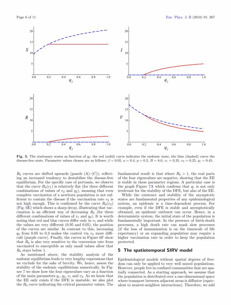
We now consider the case of varying the vaccination rateof the susceptible individuals v2 (Fig. 4). Considering firstthe EE, it can be seen that the qualitative behavior of thecurves is similar to the case of varying the fraction of vac-cinated newborns. However, for the DFE the fractions ofsusceptible and vaccinated sub-populations do not changelinearly as above, see also equation (5). In particular, therate of increase of V1 as a function of v2 starts slowingdown beyond the linear regime, meaning that it becomesincreasingly difficult to protect the population. Also, forv2 = 0, V1 = V2 and hence if the only vaccination is takingplace at birth, the fraction of vaccinated people is identicalin the endemic and disease-free states.

Finally, we discuss the case of changing the conver-sion rate from vaccinated to susceptibles (q2). The lossof protection of the vaccination plays an antagonistic roleto the vaccination rate. It is not a surprise to find thatfor the DFE, the vaccinated fraction of the populationdecreases as q2 increases. The role of q2 in the equationfor S1 is the same as v2 in the equation for V1 [Eq. (5)].For the EE, though, the situation is slightly different.While the infected fraction of the population increases

Eur. Phys. J. B (2018) 91: 267 Page 5 of 11

0.0 0.2 0.4 0.6 0.8 1.0

5

10

15

20

0.0 0.2 0.4 0.6 0.8 1.0

5

10

15

20

0.0 0.2 0.4 0.6 0.8 1.0

5

10

15

20

0.0 0.2 0.4 0.6 0.8 1.0

5

10

15

20

v2

v2

v2

v2

S I

R V

Fig. 4. The stationary states as function of v2: the red (solid) curve indicates the endemic state, the blue (dashed) curve thedisease-free state. Other parameters used are as follows: β = 0.05, a = 0.4, p = 0.3, B = 8.0, v1 = 0.35, q1 = 0.45, q2 = 0.15.

with q2, it does so at a rate that is slower than the lineargrowth rate at onset, showing that a waning immunizationfavors the endemic state, but a change in this parameteris less dangerous than a decrease of any of the vaccinationparameters.

A relevant quantity in epidemiology is the basic repro-duction number R0. It is defined as the expected numberof secondary individuals infected by an individual in itslifetime (for a review see Ref. [24]). This quantity helpsto predict whether a disease present in a population willcreate an epidemic (if R0 > 1).

To calculate the basic reproduction number R0, weuse the next generation method for structured popula-tions [24]. For that we separate the Jacobian given inequation (7) into a transmission part T and transitionpart Σ, evaluated at the DFE. We obtain:

T =

0 −βS1 0 00 βS1 0 00 0 0 00 0 0 0

(10)

and

Σ =

−v2 − p 0 q1 q20 −a− p 0 00 a −q1 − p 0v2 0 0 −q2 − p

. (11)

Then, R0 is the leading eigenvalue of the matrix [−TΣ−1].It is determined as

R0 =Bβ(q2 + p− pv1)

p(a+ p)(q2 + v2 + p). (12)

The R0 shown in equation (12) above is identical to S1/S2

and to β/βc, providing alternative interpretations of theonset of an epidemic. Also, R0 = 1 + (a + p)−1λ4, elu-cidating the relationship between the basic reproductionnumber and the dominant eigenvalue of the stability anal-ysis of the DFE. Because of this link it is not surprisingthat for this model, the same result can be obtained byevaluating λ4 or by setting I2 to zero.

Figure 6 shows R0 as a function of the vaccinationparameters v1, v2, and the rate of loss of protection q2.The panels (A)–(C) exhibit a situation involving an epi-demic with low R0, while panels (D)–(F) use parametervalues for pertussis, a disease with high R0. In agreementwith the above figures for the stationary states, we observethat for low vaccination rates (v1, v2) and a high rate ofloss of protection (q2), the endemic state is stable whilethe disease-free state is unstable. On the other hand, if thevaccinated fraction of the population loses its protectionat a high rate, a transition from the disease-free state tothe endemic equilibrium occurs. Only the dependence ofR0 on v1 is linear. As the infection rate β increases, the

Page 6 of 11 Eur. Phys. J. B (2018) 91: 267

0.0 0.2 0.4 0.6 0.8 1.0

5

10

15

20

0.0 0.2 0.4 0.6 0.8 1.0

5

10

15

20

0.0 0.2 0.4 0.6 0.8 1.0

5

10

15

20

0.0 0.2 0.4 0.6 0.8 1.0

5

10

15

20

q2

q2

q2

q2

S I

R V

Fig. 5. The stationary states as function of q2: the red (solid) curve indicates the endemic state, the blue (dashed) curve thedisease-free state. Parameter values chosen are as follows: β = 0.05, a = 0.4, p = 0.3, B = 8.0, v1 = 0.35, v2 = 0.25, q1 = 0.45.

R0 curves are shifted upwards (panels (A)–(C)), reflect-ing an increased tendency to destabilize the disease-freeequilibrium. For the specific case of pertussis, we observethat the curve R0(v1) is relatively flat (for three differentcombinations of values of v2 and q2), meaning that evencomplete vaccination of a newborn population is not suf-ficient to contain the disease if the vaccination rate v2 isnot high enough. This is confirmed by the curve R0(v2)(Fig. 6E) which shows a sharp decay, illustrating that vac-cination is an efficient way of decreasing R0 (for threedifferent combinations of values of v1 and q2). It is worthnoting that red and blue curves differ only in v1 and whilethe values are very different (0.95 and 0.05), the positionof the curves are similar. In contrast to this, increasingq2 from 0.05 to 0.3 makes the control via v2 more diffi-cult (purple curve). Finally, the curves in Figure 6F showthat R0 is also very sensitive to the conversion rate fromvaccinated to susceptible as only small values allow thatR0 stays below 1.

As mentioned above, the stability analysis of theendemic equilibrium leads to very lengthy expressions thatwe exclude for the sake of brevity. We, hence, assess thestability of the endemic equilibirium numerically. In Fig-ure 7 we show how the four eigenvalues vary as a functionof the main parameters q1, q2, v1 and v2. As we know thatthe EE only exists if the DFE is unstable, we also plotthe R0 curve indicating the critical parameter values. The

fundamental result is that where R0 > 1, the real partsof the four eigenvalues are negative, showing that the EEis stable in these parameter regions. A particular case isthe graph Figure 7A which confirms that q1 is not onlyirrelevant for the stability of the DFE, but also of the EE.

While the existence and stability of the asymptoticstates are fundamental properties of any epidemiologicalsystem, an epidemic is a time-dependent process. Forexample, even if the DFE is stable and asymptoticallyobtained, an epidemic outburst can occur. Hence, in adeterministic system, the initial state of the population isfundamentally important. In the presence of birth-deathprocesses, a high death rate can mask slow processes(if the loss of immunization is on the timescale of lifeexpectancy) or an expanding population may require ahigher vaccination rate in order to keep the populationprotected.

5 The spatiotemporal SIRV model

Epidemiological models without spatial degrees of free-dom can only be applied to very well mixed populations.However, people live in confined communities that are spa-tially connected. As a starting approach, we assume thatthe population is distributed over a one-dimensional spacewhere transport between adjacent areas is diffusive (equiv-alent to nearest-neighbor interactions). Therefore, we add

Eur. Phys. J. B (2018) 91: 267 Page 7 of 11

v1

R0

A B C

R0

R0

v2 q

2

0.0 0.2 0.4 0.6 0.8 1.0

0.5

1.0

1.5

2.0

0.0 0.2 0.4 0.6 0.8 1.0

0.5

1.0

1.5

2.0

0.0 0.2 0.4 0.6 0.8 1.0

0.5

1.0

1.5

2.0

v1

D E F

v2 q

2

R0

R0

R0

0.0 0.2 0.4 0.6 0.8 1.0

5

10

15

0 1 2 3 4 5

5

10

15

0.0 0.5 1.0 1.5 2.0

5

10

15

Fig. 6. (A)–(C) The basic reproduction number R0 (which is not the same as the initial condition of the number of recoveredagents in a simulation) as function of the parameters v1 (A), v2 (B) and q2 (C), and each for three values of the infectionrate, β = 0.03 (blue), β = 0.05 (red) and β = 0.07 (green). The curve R0 = 1 is shown as a thin grey dotted curve. Comparealso with Figures 3–5. Other parameter values are as follows: a = 0.4, p = 0.3, B = 8.0, v1 = 0.35, v2 = 0.25, q1 = 0.45,q2 = 0.15. (D-F) The basic reproduction number R0 as function of the parameters v1 (D), v2 (E) and q2 (F) for a parameter setdescribing pertussis infection (parameters taken partially from [31] and chosen such that an uncontrolled R0 (no vaccination) isaround 16). In (D), following curves are shown: v2 = 0.3, q2 = 0.05 (red solid curve), v2 = 0.8, q2 = 0.05 (green dashed curve)and v2 = 0.3, q2 = 0.3 (purple dot-dashed curve). In (E), following curves are shown: v1 = 0.95, q2 = 0.05 (red solid curve),v1 = 0.05, q2 = 0.05 (blue dot-dashed curve) and v1 = 0.95, q2 = 0.3 (purple dot-dashed curve). In (F), following curves areshown: v1 = 0.95, v2 = 0.3 (red solid curve), v1 = 0.95, v2 = 0.8 (green dashed curve) and v1 = 0.05, v2 = 0.3 (blue dot-dashedcurve). The other parameters are β = 140, p = 1/70, B = 0.026, q1 = 0.1 (assuming that time is measured in years) and thecurve R0 = 1 is shown as a thin grey dotted curve.

diffusion terms to the SIRV model (2) and obtain

∂S

∂t= B(1− v1)− βSI − v2S + q1R+ q2V − pS

+DS∇2S, (13a)

∂I

∂t= βSI − aI − pI +DI∇2I, (13b)

∂R

∂t= aI − q1R− pR+DR∇2R, (13c)

∂V

∂t= v1B + v2S − q2V − pV +DV ∇2V , (13d)

where DF (F = S, I, R, V ) are diffusion constants for sus-ceptible, infected, recovered and vaccinated individuals,respectively.The two fixed points shown in equations (5) and (6) of

the diffusion-free system are solutions of the system withdiffusion (13) in case the variables do not show any spa-tial dependence, i.e., represent a homogeneous solution.However, the linear stability of this homogeneous solutiondepends on diffusion, as we shall see now.

Perturbed around the homogeneous fixed points, inthe Fourier transformed (k, t) space, the dynamics isrepresented through the Jacobian Jk that is given by

See equation (14) next page

where I∗ and S∗ need to be replaced by the respectivestationary state solution [equations (5), (6)]. Around thedisease-free steady state, one can find the eigenvalues asfollows

See equation (15) next page.

The eigenvalue λ1(k) is a generalization of λ2 of the ODEsystem and is always negative. The eigenvalue λ2(k) is thegeneralization of λ4 of the ODE system and can there-fore change sign. The eigenvalues λ3,4(k) depend on thesum and differences of the diffusion coefficients of the sus-ceptible and vaccinated population fractions. It can beeasily shown that λ3,4(k) are always negative and hencediffusion has always a stabilising effect on the DFE. Themost unstable wavenumber is k = 0. Hence, whenever the

Page 8 of 11 Eur. Phys. J. B (2018) 91: 267

Jk =

−(βI∗ + v2 + p+DSk2) −βS∗ q1 q2

βI∗ −(−βS∗ + a+ p+DIk2) 0 0

0 a −(q1 + p+DRk2) 0

v2 0 0 −(q2 + p+DV k2)

, (14)

λ1(k) = −q1 − p−DRk2, (15a)

λ2(k) = −a− p+Bβ(q2 + p− pv1)

p(q2 + v2 + p)−DIk

2, (15b)

λ3(k) =1

2

[− 2p− (DS +DV )k2 − q2 − v2

+

√[q2 − (DS −DV )k2]

2+ 2[(DS −DV )k2 + q2]v2 + v22

], (15c)

λ4(k) =1

2

[− 2p− (Ds +DV )k2 − q2 − v2

−√

[q2 − (DS −DV )k2]2

+ 2[(DS −DV )k2 + q2]v2 + v22]. (15d)

DFE is unstable in the purely temporal system, it is alsounstable in the spatiotemporal system.

Figure 8 shows a numerical simulation of the spa-tiotemporal SIRV model [Eqs. (13)] in one-dimensionalspace. The initial condition is a disease-free state witha small nucleus of infected agents at the center of themedium. Parameters have been chosen to ensure that thedisease-free state is unstable, leading to a transition tothe endemic state. This can be clearly seen as a travelingwave in the space-time plot for I in Figure 8A. Figures 8Band 8C illustrate the behavior of all variables for a fixedpoint in space (B) and for a fixed point in time (C). Thelatter displays the profile of the traveling wave front. Forthis set of parameters, the spatial distribution for I showssmall peaks in the fronts.

The wave of infection observed in Figure 8 can be inves-tigated in more detail. In Figure 9, we show how the frontvelocity changes with the diffusion constant DI and theinfection rate β. Both functional forms follow a square rootdependence reminiscent of the Fisher-Kolmogorov equa-tion [14,25]. Indeed, for a single-species population modelwith variable u, it is known that the natural front velocityof a front triggering a transition from the unstable to thestable state is given by v = 2

√f ′(u1)D, where D is the

diffusion constant, f(u) describes the temporal dynamicsand u1 is the unstable steady state [25]. Applying the samerationale to equation (2b), we obtain

v = 2√

(βS1 − a− p)DI = 2√

(β − βc)S1DI . (16)

The qualitative agreement between the curves is surpris-ingly good which is remarkable as no fitting parametersare applied and the analytic expression uses only one equa-tion of a coupled 4-dimensional dynamical system. Thereis a slight quantitative difference for small velocities, asseen in Figure 9A that could be partially explained by the

fact that the simulations are performed in a finite sizedsystem and that the calculation of the front speed fromthe simulation data carries an error.

6 Discussion

In this article, we have considered an SIRV model in thetemporal and spatiotemporal domain. The model has twoasymptotic states, the disease-free state and the endemicstate. We have focused on the consequences of diminishingimmunization, i.e., the effect when vaccinated or recoveredindividuals become susceptible again. The results havebeen obtained through bifurcation analysis of the individ-ual solutions (for S, I, R and V ), as well as through thedetermination of the basic reproduction number R0. In theasymptotic regime the number of each sub-populations isproportional to its density in the whole population, so theresults refer directly to population densities or fractions.Our exclusively temporal model shares similarities with amodel studied in [23], however, the models only coincideif we set v1 = q1 = 0 in our model and simultaneouslyset µ = σ = 0 in the model discussed in reference [23].However, assuming non-zero values for these parameter iscrucial for both our model (possible vaccination at birthand conversion from recovered to susceptible agents) andthe model discussed in reference [23] (variable vaccine effi-cacy and possibility of disease-induced deaths) and hencethe interpretation and applicability of the models differsubstantially.

By considering the results of a linear stability analy-sis of the disease-free state, we have found that the lossof protection of the recovered fraction of the population(with rate q1) has no influence on the onset of the endemicstate. While the rate q1 does not influence the asymptoticDFE, it can impact on the transient time to equilibrium.

Eur. Phys. J. B (2018) 91: 267 Page 9 of 11

q1

v2

v1

q2

1 2 3 4 5

- 2

- 1

1

2

1 2 3 4 5

- 2

- 1

1

2

0.2 0.4 0.6 0.8 1.0

- 2

- 1

1

2

1 2 3 4 5

- 2

- 1

1

2

A B

C D

Fig. 7. Stability of the endemic equilibrium. We show the real parts of the four eigenvalues as function of the parameters q1(A), q2 (B), v1 (C) and v2 (D), together with the curve for R0 (black) indicating the stability of the DFE (the dotted line atR0 = 1 is a guide to the eye). Where the DFE is unstable, the EE is stable. Other parameter values are as follows: a = 0.4,β = 0.05, p = 0.3, B = 8.0, v1 = 0.35, v2 = 0.25, q1 = 0.45, q2 = 0.15.

A B C

t x0 10 20 30 40 50

5

10

15

20

x

t- 100 - 50 0 50 100

5

10

15

20

Fig. 8. Wave of an epidemic spread as observed in the SIRV model. (A) Space-time density plot for I. (B) Temporal variationof {S, I, R, V } at the centre of the simulation domain considered (x = 0). (C) Front profile of {S, I, R, V } at t = 100. The brown(dashed) curve denotes S, the red (dot-dashed) curve denotes I, the green (dotted) curve denotes R and the blue (solid) curverepresents V . Parameters used are as follows: β = 0.05, a = 0.4, p = 0.3, B = 8.0, v1 = 0.25, v2 = 0.15, q1 = 0.45, q2 = 0.25,DS = 10, DI = 0.5, DR = 10, DV = 10. The system size is −100 ≤ x ≤ 100, the boundary conditions are periodic and thedisplayed time interval in (A) is T = 180.

Page 10 of 11 Eur. Phys. J. B (2018) 91: 267

Fig. 9. Wave speed of an epidemic in the SIRV model as afunction of DI (A) and β (B). Speeds are measured from thesimulation data (black solid curves) and compared with equa-tions (16) (red dashed curves). No fitting parameters are used.Other parameters are as in Figure 8.

On the other hand, the loss of protection of the vacci-nated fraction of the population (with rate q2) can shiftthe population from a disease-free state to an endemicone. An interesting feature of this model is that the den-sity of susceptibles in the endemic regime does not dependon q2. The curve of R0 with q2 is increasing, however,with a decreasing slope, meaning that decreasing q2 inthe epidemic regime may bring the population closer tothe threshold than predicted by a linear regression. Con-sidering the effect of the vaccination rates, we find that thefraction of vaccinated newborns v1 changes the asymptoticfractions linearly in both stationary states, as well as R0.This is in contrast to v2 where the dependence is non-linear. There, we have found that if v2 is decreased in andisease-free state, the basic reproduction number increasesmore strongly than predicted by a linear regression. Thisimplies that the critical R0 = 1 may be reached for higherv2 than assumed.

Our results show that in the diffusion-free statethe dominant eigenvalue of the disease-free state λ4 =β(q2 + p)(a+ q1 + p)

q2 + v2 + pI2. This means that if the endemic

state exists, the disease-free equilibrium is unstable thatis associated with positive λ4 values and R0 > 1. In thecomplete absence of adult vaccination, implying v2 = 0,equations (5) and (6) show that the vaccinated num-ber density is the same for the two asymptotic states(Bv1q2 + p

). This then implies that one cannot predict

the actual epidemic state from the proportion of thevaccinated population alone. We have presented a numer-ical solution for the stability problem of the endemicequilibrium. It indicates that while the EE exists, it isstable.

The features obtained from a study of this model canbe put in the appropriate context of epidemiological data.Diphtheria and Pertussis (whooping cough) are amongstthe diseases that are associated with waning immuniza-tion. Repeated vaccinations (“boosts”) are needed toprevent the spreading of such diseases. Due to the highR0 values of these diseases, children are vaccinated at

early ages. Without epidemiological control, the R0 of per-tussis has been estimated at 16–18 [26], a value loweredto 11–15 [27] later. In the presence of vaccination, thevalue could be lowered to around 5.5 [28]. The incidenceamong adults are explained by waning immunization andthe possibility of evolving subclinical strains that are heldresponsible for persistence of pertussis in vaccinated pop-ulations [28]. In Figure 10, we show a short time seriesof a population suffering from pertussis infection and forwhich the endemic equilibrium is stable. The initial stateconsists of a population with very few infected agents. Weclearly notice some outbursts of infection, with a charac-teristic time gap between 1 and 2 years. This timescaleis not far off from known deterministic models of pertus-sis which consistently predict annual epidemics [29]. Note,however, that detailed and more realistic models for per-tussis rely on an SEIR mechanism, with an exposed/latentphase and/or age structure, and possibly term-time forc-ing. Furthermore, stochastic effects are also known to becrucial in the disease dynamics [30]. A recent work com-pares the different classes of models including reinfectionof recovered and loss of infection-derived immunity andsubsequent reinfection [31]. In the context of this arti-cle, we simply want to illustrate an example of a specificdisease for our model.

For all realistic epidemiological models, spatial inter-actions have to be considered. In our model, we haveassumed a nearest-neighbor interaction, modeled by dif-fusion terms. Our linear stability analysis of the DFEconfirms that the most unstable wavenumber is k = 0, andthat the disease-free equilibrium cannot be destablized bycontrolling the diffusion rates. A discussion of the spatialstability problem of the endemic equilibrium is beyond thescope of the present work.

A well-known feature of infection models with dif-fusion is that they are able to describe the propaga-tion of waves, of particular interest being waves thatrepresent the onset of an epidemic. We have shownthat in spite of the comparatively high complexity ofthe model (4 coupled equations), the wave speed stillapproximately follows the one-species Fisher-Kolmogorovmodel, similar to what has been observed for a differentmodel [16].

Temporal and spatiotemporal epidemiological modelshave been studied in many variants. A series of recentworks tries to find optimal vaccination strategies, forexample by a probabilistic modelling of infection in net-works [32], by minimizing the number of infected andsusceptibles [33], by a Poisson distributed vaccinationschedule on networks [6], by an information (and time)dependent vaccination rate [10], or by optimizing thevaccination rate through a stochastic maximum princi-ple [12]. In contrast to these articles, we analyze thefront speed of a general SIRV model, similar to theapproaches of [18] for a stochastic SIR model and [20] foran SIR model with non-smooth treatment (vaccination)functions.

As possible follow-up, we mention the spatial stabil-ity analysis of the endemic equilibrium, an analytical andnumerical investigation of fronts in two space dimensionsand the incorporation of social effects.

Eur. Phys. J. B (2018) 91: 267 Page 11 of 11

t

B

t0 1 2 3 4 5

2

4

6

8

10

12

0 1 2 3 4 5

2

4

6

8

10

12

Fig. 10. Initial temporal dynamics of the fractions of infected (solid curve) and susceptibles (dashed curve) for a parameter setfor pertussis (time unit is years): p = 1/70, r = 140, a = 365/23, B = 0.026, v1 = 0.95, q1 = 0.1, q2 = 0.05 and v2 = 0 (A) andv2 = 0.3 (B). The dynamics is characterised by damped oscillations before settling to the endemic equilibrium.

The authors acknowledge some preliminary simulations byAsad Ahmad. M.S. would like to thank EPSRC for fundingvia the grant EP/M02735X/1.

Author contribution statement

All authors conceived the presented idea. E.G. and M.S.performed the computations. M.S. and A.K.C. wrote thefinal manuscript.

Open Access This is an open access article distributedunder the terms of the Creative Commons AttributionLicense (http://creativecommons.org/licenses/by/4.0), whichpermits unrestricted use, distribution, and reproduction in anymedium, provided the original work is properly cited.

References

1. W.O. Kermack, A.G. McKendrick, Proc. Roy. Soc. A 115,700 (1927)

2. K. Rock, S. Brand, J. Moir, M.J. Keeling, Rep. Prog. Phys.77, 026602 (2014)

3. H.W. Hethcote, SIAM Rev. 42, 599 (2000)4. A. Scherer, A. McLean, Brit. Med. Bull. 62, 187 (2002)5. J. Verdasca, M.M.T. da Gama, A. Nunes, N.R.

Bernardino, J.M. Pacheco, M.C. Gomes, J. Theor. Biol.233, 553 (2005)

6. L.B. Shaw, I.B. Schwartz, Phys. Rev. E 81, 046120 (2010)7. K. Sun, A. Baronchelli, N. Perra, Eur. Phys. J. B 88, 326

(2015)8. A. d’Onofrio, P. Manfredi, E. Salinelli, Math. Model. Nat.

Phenom. 2, 26 (2007)9. Z. Feng, S. Towers, Y. Yang, AAPS J. 13, 427 (2011)

10. Z. Ruan, M. Tang, Z. Liu, Phys. Rev. E 86, 036117 (2012)11. A. Kamenev, B. Meerson, Phys. Rev. E 77, 061107

(2008)

12. M. Ishikawa, Transac. ISCIE 25, 343 (2012)13. D. Walgraef, Spatio-Temporal Pattern Formation

(Springer, New York, 1997)14. A.S. Mikhailov, Foundations of Synergetics I , 2nd edn.

(Springer, Berlin, 1994)15. S. Riley, K. Eames, V. Isham, D. Mollison, P. Trapman,

Epidemics 10, 68 (2015)16. G. Abramson, V.M. Kenkre, T.L. Yates, R.R. Parmenter,

Bull. Math. Biol. 65, 519 (2003)17. L. Rass, J. Radcliff, Spatial Deterministic Epidemics

(American Mathematical Society, Providence, RI, 2003)18. U. Naether, E.B. Postnikov, I.M. Sokolov, Eur. Phys. J. B

65, 353 (2008)19. Q.X. Liu, Z. Jin, J. Stat. Mech. 2007, P05002 (2007)20. N. Hussaini, M. Winter, J. Stat. Mech. 2010, P11019

(2010)21. O. Stancevic, C.N. Angstmann, J.M. Murray, B.I. Henry,

Bull. Math. Biol. 75, 774 (2013)22. K. Capala, B. Dybiec, Eur. Phys. J. B 90, 85 (2017)23. W. Yang, C. Sun, J. Arino, J. Math. Anal. Appl. 372, 208

(2010)24. J.M. Heffernan, R.J. Smith, L.M. Wahl, J. Roy. Soc.

Interface 2, 281 (2005)25. J.D. Murray, Mathematical Biology (Springer, Berlin,

1989)26. R.M. Anderson, R.M. May, Infectious diseases of humans

(Oxford Univ. Press, Oxford, 1991)27. H.J. Wearing, P. Rohani, PLoS Pathog. 5, e1000647 (2009)28. M. Kretzschmar, P.F.M. Teunis, R.G. Pebody, PLoS Med.

7, e1000291 (2010)29. H.T.H. Nguyen, P. Rohani, J. Roy. Soc. Interface 5, 403

(2008)30. P. Rohani, M.J. Keeling, B.T. Grenfell, Am. Nat. 159, 469

(2002)31. G. Rozhnova, A. Nunes, J. R. Soc. Interface 9, 2959 (2012)32. F. Takeuchi, K. Yamamoto, J. Theor. Biol. 243, 39

(2006)33. G. Zaman, Y.H. Kang, I.H. Jung, Biosystems 93, 240

(2008)