Epidemiologic Study Designs

Jacky M Jennings, PhD, MPH

Associate Professor Associate Director, General Pediatrics and Adolescent Medicine Director, Center for Child & Community Health Research (CCHR)

Departments of Pediatrics & Epidemiology Johns Hopkins University

Learning Objectives

• Identify basic epidemiologic study designs and their frequent sequence of study

• Recognize the basic components

• Understand the advantages and disadvantages

• Appropriately select a study design

Research Question & Hypotheses

Study Design

Analytic Plan

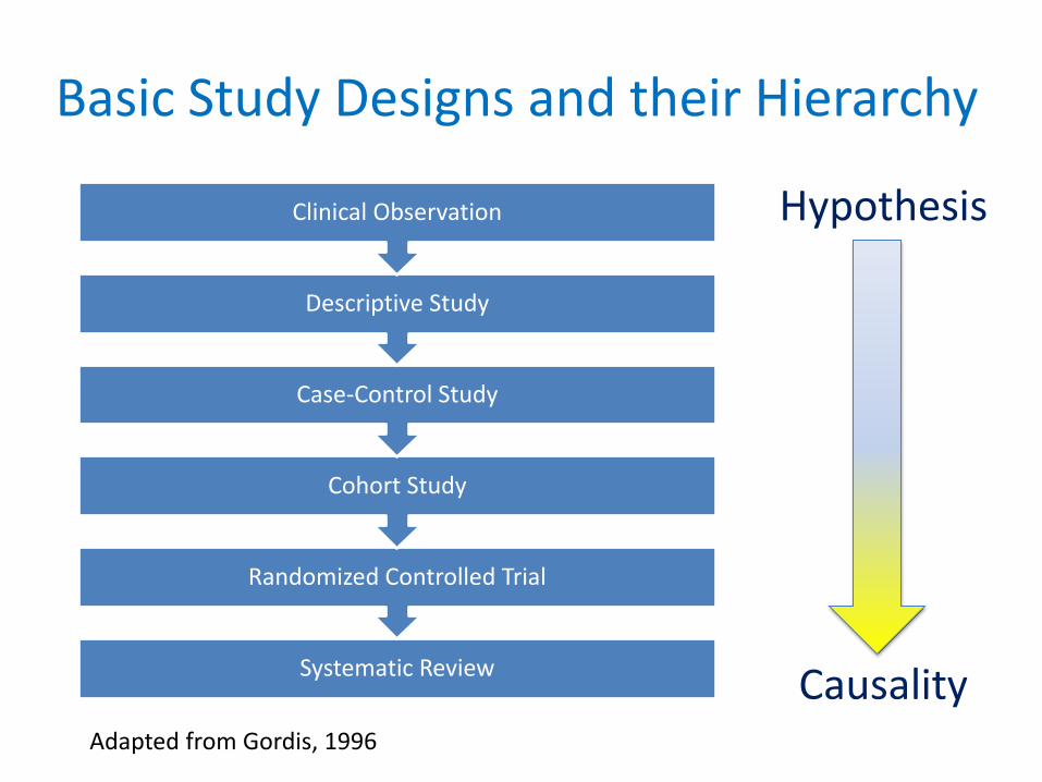
Basic Study Designs and their Hierarchy

Systematic Review

Randomized Controlled Trial

Cohort Study

Case-Control Study

Descriptive Study

Clinical Observation

Adapted from Gordis, 1996

Hypothesis

Causality

MMWR

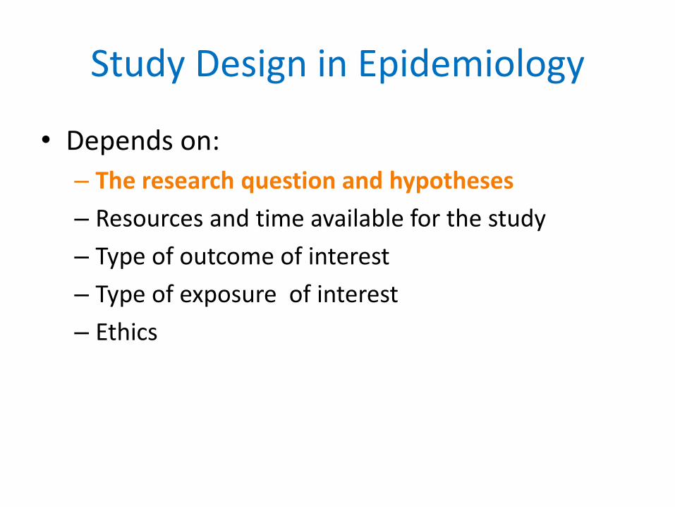
Study Design in Epidemiology

• Depends on:

– The research question and hypotheses

– Resources and time available for the study

– Type of outcome of interest

– Type of exposure of interest

– Ethics

Study Design in Epidemiology

• Includes:

– The research question and hypotheses

– Measures and data quality

– Time

– Study population

• Inclusion/exclusion criteria

• Internal/external validity

Epidemiologic Study Designs

• Descriptive studies

– Seeks to measure the frequency of disease and/or collect descriptive data on risk factors

• Analytic studies

– Tests a causal hypothesis about the etiology of disease

• Experimental studies

– Compares, for example, treatments

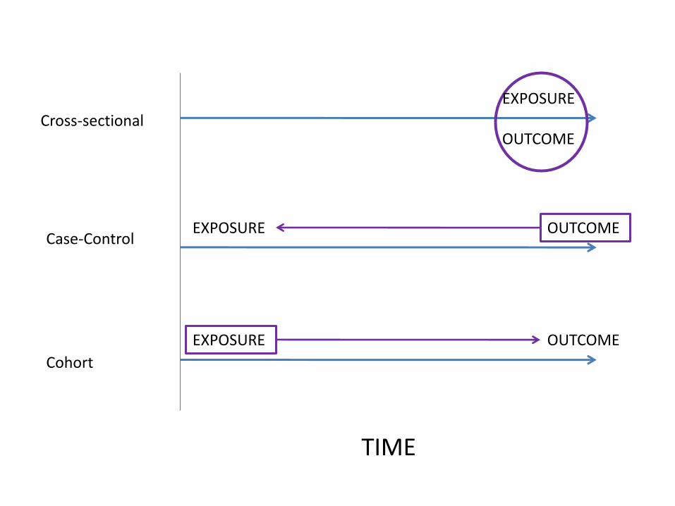
Cross-sectional

Case-Control

Cohort

TIME

EXPOSURE

OUTCOME

OUTCOME EXPOSURE

EXPOSURE OUTCOME

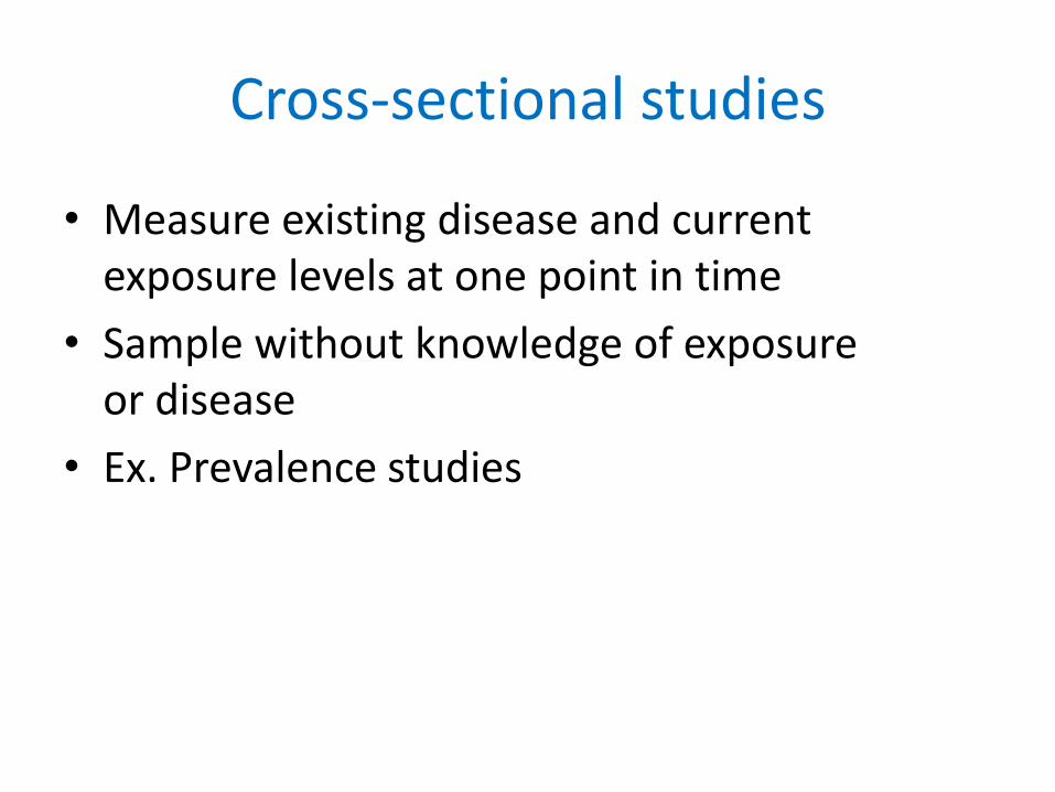
Cross-sectional studies

• Measure existing disease and current exposure levels at one point in time

• Sample without knowledge of exposure or disease

• Ex. Prevalence studies

Cross-sectional studies

• Advantages

– Often early study design in a line of investigation

– Good for hypothesis generation

– Relatively easy, quick and inexpensive…depends on question

– Examine multiple exposures or outcomes

– Estimate prevalence of disease and exposures

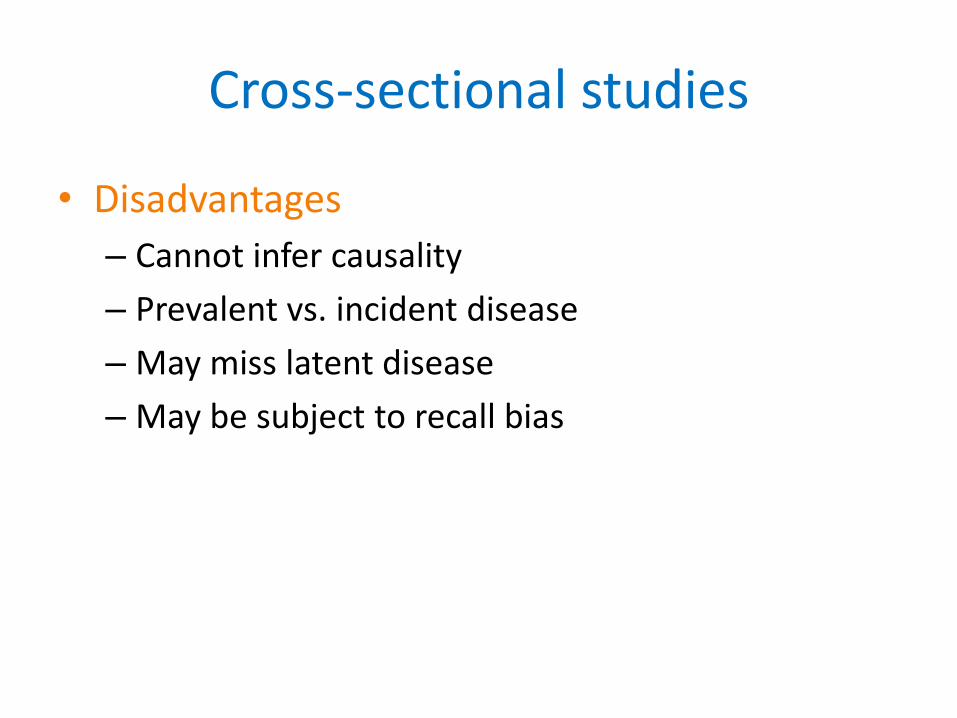
Cross-sectional studies

• Disadvantages

– Cannot infer causality

– Prevalent vs. incident disease

– May miss latent disease

– May be subject to recall bias

Research Question

• Determine whether there are differences in rates of stroke and myocardial infarction by gender and race among patients.

Hypothesis

• There will be differences in rates of stroke by gender and race.

• There will be differences in rates of myocardial infarction by gender and race.

Case-Control studies

• Identify individuals with existing disease/s and retrospectively measure exposure

Population

Cases

Controls

Exposed

Not exposed

Exposed

Not exposed

Time

Case-Control studies

• Advantages

– Good design for rare, chronic and long latency diseases

– Relatively inexpensive (population size and time)

– Allows for the examination of multiple exposures

– Estimate odds ratios

– Hospital-based studies and outbreaks

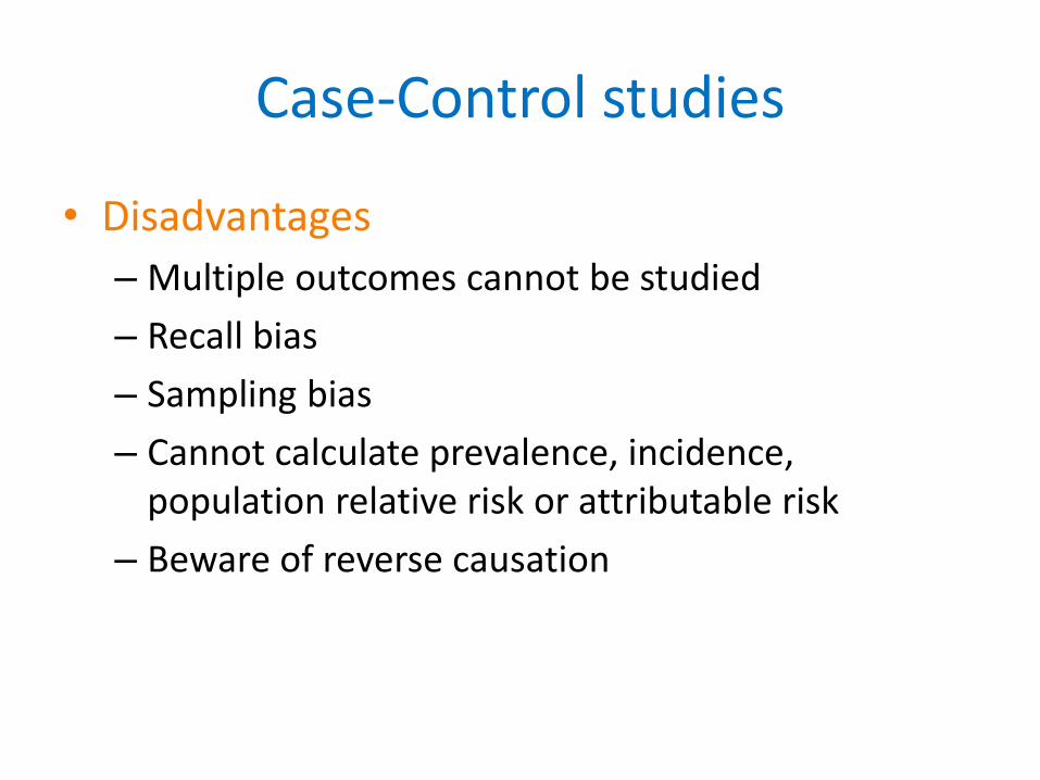
Case-Control studies

• Disadvantages

– Multiple outcomes cannot be studied

– Recall bias

– Sampling bias

– Cannot calculate prevalence, incidence, population relative risk or attributable risk

– Beware of reverse causation

Neonatal Abstinence Syndrome (NAS) and Drug Exposure

Research question

?

Hypothesis 1

Buprenorphine-exposed neonates will exhibit

less NAS than methadone-exposed neonates.

Case-Control Study Example

• Hypothesis 1: Buprenorphine-exposed neonates will exhibit less NAS than methadone-exposed neonates.

Neonates

NAS

Non-NAS

Metha-done

Metha-done

Bupren- orphine

Bupren- orphine

Challenges in Case-Control Studies

• Selection of Controls

– Sample size

– Matching (group or individual)

• Selection of Cases

– Incident or prevalent disease

• Nested case-control study

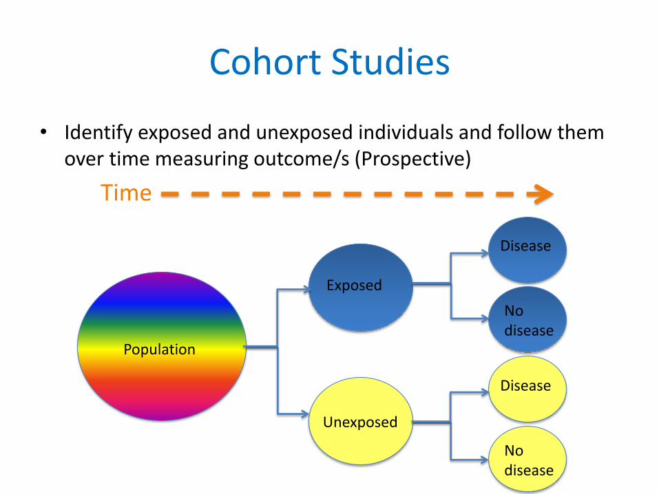
Cohort Studies

Population

Unexposed

Exposed

No disease

Disease

No disease

Disease

Time

• Identify exposed and unexposed individuals and follow them over time measuring outcome/s (Prospective)

Prospective Cohort Study

study starts exposure disease

Time

Time

exposure study starts disease

Retrospective Cohort Study

exposure disease study starts

Time

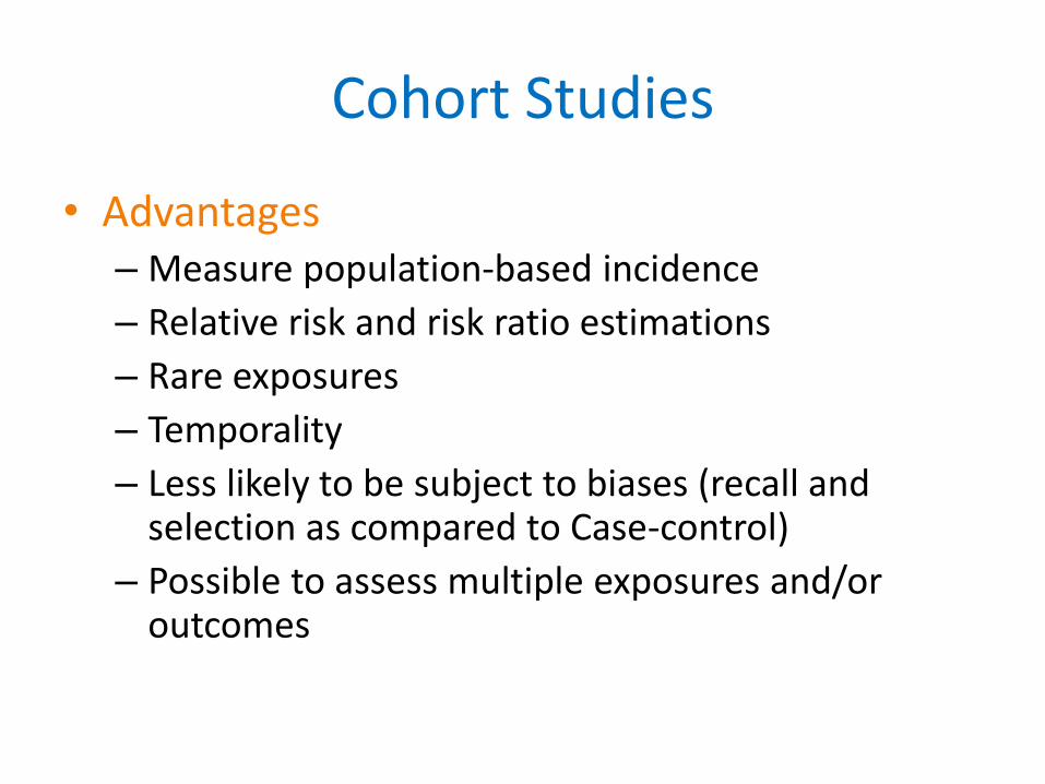
Cohort Studies

• Advantages – Measure population-based incidence

– Relative risk and risk ratio estimations

– Rare exposures

– Temporality

– Less likely to be subject to biases (recall and selection as compared to Case-control)

– Possible to assess multiple exposures and/or outcomes

Cohort Studies

• Disadvantages – Impractical for rare diseases and diseases with a

long latency

– Expensive • Often large study populations

• Time of follow-up

– Biases • Design - sampling, ascertainment and observer

• Study population – non-response, migration and loss-to-follow-up

Research Question Determine whether circulating biomarkers (i.e. C-reactive protein; exhaled breath condensate - pH, hydrogen peroxide, 8-isoprostene, nitrite, nitrate levels; sputum - TNF-, IL-6, IL-8, IL-1, neutrophil elastase; and fractional exhaled nitric oxide) predict individuals who will benefit from initiation of antibiotic therapy for the treatment of a mild decrease in FEV1. Hypothesis Biomarkers at the time of presentation with a mild increase in pulmonary symptoms or small decline in FEV1 can be used to identify which patients require antibiotics to recover.

Individuals with exacerbation with cystic fibrosis (CF)

No-biomarker

biomarkers

No response

Response to antibiotic

therapy

Baseline days weeks

Cohort Study

Important features

• How much selection bias was present? – Were only people at risk of the outcome included? – Was the exposure clear, specific and measureable? – Were the exposed and unexposed similar in all

important respects except for the exposure?

• Were steps taken to minimize information bias? – Was the outcome clear, specific and measureable? – Was the outcome identified in the same way for both

groups? – Was the determination of the outcome made by an

observer blinded to treatment?

Important features

• How complete were the follow-up of both groups? – What efforts were made to limit loss to follow-up?

– Was loss to follow-up similar in both groups?

• Were potential confounding factors sought and controlled for in the study design or analysis? – Did the investigators anticipate and gather

information on potential confounding factors?

– What methods were used to assess and control for confounding?

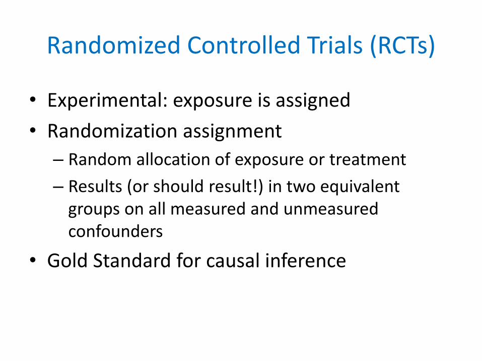
Randomized Controlled Trials (RCTs)

• Experimental: exposure is assigned

• Randomization assignment

– Random allocation of exposure or treatment

– Results (or should result!) in two equivalent groups on all measured and unmeasured confounders

• Gold Standard for causal inference

Randomized Controlled Trials

• Advantages – Least subject to biases of all study designs

(IF designed and implemented well…!)

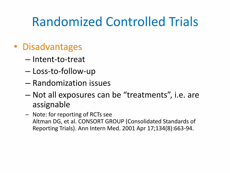
Randomized Controlled Trials

• Disadvantages – Intent-to-treat

– Loss-to-follow-up

– Randomization issues

– Not all exposures can be “treatments”, i.e. are assignable

– Note: for reporting of RCTs see Altman DG, et al. CONSORT GROUP (Consolidated Standards of Reporting Trials). Ann Intern Med. 2001 Apr 17;134(8):663-94.

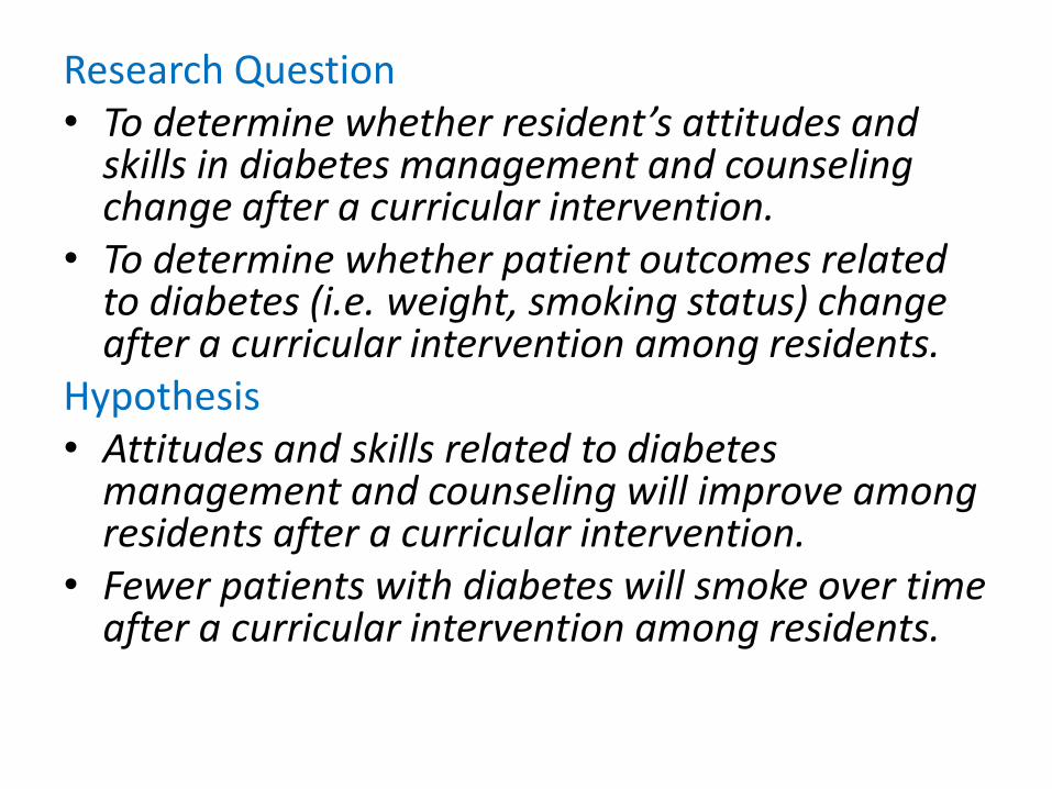
Research Question • To determine whether resident’s attitudes and

skills in diabetes management and counseling change after a curricular intervention.

• To determine whether patient outcomes related to diabetes (i.e. weight, smoking status) change after a curricular intervention among residents.

Hypothesis • Attitudes and skills related to diabetes

management and counseling will improve among residents after a curricular intervention.

• Fewer patients with diabetes will smoke over time after a curricular intervention among residents.

Randomization Strategies

• Randomly assigned

• Quasi-randomization

• Block randomization – method of randomization that ensures that at any point in the trial, roughly equal numbers of participants have been allocated to the comparison groups

Grimes & Schulz, 2002

Study Design

• Must be defensible

• Drives conclusions: What do you want to be able to say at the end of the study?

Exploratory Data Analyses

Jacky M Jennings, PhD, MPH

Objectives

• To identify some basic steps in data analyses

• To understand the reason for and methods of exploratory quantitative data analysis

• To learn some statistical tools for inferential statistics

Research Questions

• Testable hypotheses

• Measureable – exposure and outcome

• Time - how is time incorporated

• Study population

Taking Stock of your Data

• How was the data measured?

– Type of data (i.e. continuous, dichotomous, categorical, etc.)

– Single item, multiple items, new/previously validated measure

– Cross-sectional vs. cohort study (i.e. one measure in time vs. multiple measures over time)

Descriptive Statistics

• Exploratory data analysis (EDA)

• Basic numerical summaries of data (i.e. Table 1 in a paper)

• Basic graphical summaries of data

• Goal: to visualize relationships and generate hypotheses

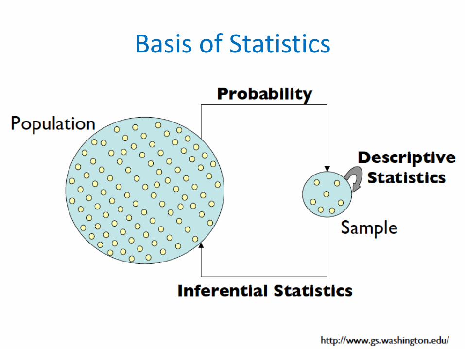
Basis of Statistics

Exploratory Data Analysis (EDA)

• Essential first step of data analysis

• Helps to:

– Identify errors

– Visualize distributions and relationships

– See patterns, e.g. natural or unnatural

– Find violations of statistical assumptions

– Generate hypotheses

Loo

k

Total 42 42 42 42 42 210 . 10 4 4 7 10 35 1.236 0 0 1 0 0 1 1.03 0 0 0 0 1 1 .985 0 1 0 0 0 1 .904 0 1 0 0 0 1 .651 0 0 1 0 0 1 .574 0 0 1 0 0 1 .566 0 0 1 0 0 1 .35 0 0 0 0 1 1 .328 0 0 0 1 0 1 .303 0 0 0 1 0 1 .29 0 0 0 1 0 1 .262 0 0 1 0 0 1 .223 1 0 0 0 0 1 .204 0 0 0 0 1 1 .172 0 0 0 0 1 1 .164 0 1 0 1 0 2 .141 1 0 0 0 0 1 .138 0 1 0 0 0 1 .137 1 0 0 0 0 1 .12 0 0 0 1 0 1 .119 0 0 0 0 1 1 .11 0 0 1 0 0 1 .106 0 0 0 1 0 1 .105 1 0 0 0 0 1 .102 0 0 1 0 0 1 .098 1 0 0 0 0 1 .095 0 0 0 1 0 1 .092 0 0 0 0 1 1 .089 1 0 0 0 0 1 .081 0 1 0 0 0 1 .08 0 0 0 0 1 1 .074 1 0 0 0 0 1 .069 1 0 0 0 0 1 .065 0 1 0 0 0 1 .063 0 0 0 0 1 1 .054 0 0 0 0 1 1 .053 0 1 0 0 0 1 .052 0 0 0 1 0 1 .049 0 0 1 0 0 1 .048 1 0 0 0 0 1 .046 0 0 0 1 1 2 .042 1 0 0 0 0 1 .04 3 1 1 0 2 7 0 19 30 29 26 20 124 GFAP 0 1 2 3 4 Total gfaptime

Types of Data

Quantitative Categorical

Binary Continuous Discrete Nominal Ordinal

Numerical Summaries of Data

• Central tendencies measures – Calculated to create a “center” around which

measurements in the data are distributed

• Variation or variability measures – Describe how far away (or data spread)

measurements are from the center

• Relative standing measures – Describe the position (or standing) of specific

measurements within the data

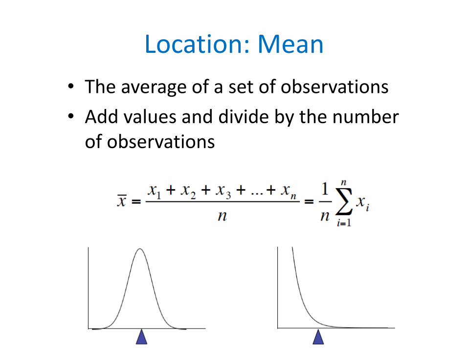
Location: Mean

• The average of a set of observations

• Add values and divide by the number of observations

Location: Median

• The exact middle value, i.e. 50th percentile

• Number of observations

– Odd: find the middle value

– Even: find the middle two values and average them

• Example

– Odd: 5, 6, 10, 3, 4, median = 10

– Even: 5, 6, 10, 8, 3, 4, median = 10+8/2= 9

Which Measure is Best?

• Mean

– best for symmetric (or normal) distributions

• Median

– Useful for skewed distributions or data with outliers

Biomarker – one time point 0

.51

1.5

Den

sity

0 1 2 3 4 5numeric rewarming_gfap

Examples of Numerical Summaries

gfap4 18 .1189444 .2465624 0 1.03 gfap3 17 .0884706 .1164072 0 .328 gfap2 20 .1795 .3286394 0 1.236 gfap1 21 .1107143 .281544 0 .985 gfap0 16 .0484375 .0686838 0 .223 Variable Obs Mean Std. Dev. Min Max

-> pvl = case

gfap4 14 .0106429 .0216603 0 .063 gfap3 18 0 0 0 0 gfap2 18 0 0 0 0 gfap1 17 .0061765 .0179869 0 .065 gfap0 16 .0231875 .0357122 0 .105 Variable Obs Mean Std. Dev. Min Max

-> pvl = control

Transformation

0.2

.4.6

.81

0 50 100 150

cubic

0.2

.4.6

.81

0 5 10 15 20 25

square

0.2

.4.6

.8

0 1 2 3 4 5

identity

0.1

.2.3

0 .5 1 1.5 2 2.5

sqrtFrac

tion

gfapHistograms by transformation

Scale: Variance

• Average of the squared deviations of values from the mean

• Example, sample variance

Scale: Standard Deviation

• Variance is somewhat arbitrary

• Standardizing helps to bring meaning to deviation from the mean

• Standard deviations are simply the square root of the variance

• Example, sample SD

Scale: Quartiles and Inter Quartile Range (IQR)

• Quartiles or percentiles (order data first)

– Q1 (1st quartile) or 25th percentile is the value for

which 25% of the observations are smaller and 75% are greater

– Q2 is the median or the value where 50% of the observations are smaller and 50% are greater

– Q3 is the value where 75% of the observations are smaller and 25% are greater

IQR

Graphical Summaries of Data: Box Plots and Histograms

• Box plot (i.e. box-and-whisker plots)

– Shows frequency or proportion of data in categories, i.e categorical data

– Visual of frequency tables

• Histogram

– Shows the distribution (shape, center, range, variation) of continuous variables

– Bin size is important

Box Plot

Upper fence

Q3 = upper hinge

Q2 = median

Q1 = lower hinge

Lower fence

Box Plot

36493841713710484070

728228127314878

74

57491178

56

5848

12

1

74

12737278

58

74

01

23

45

gfap

pre cooling rewarming post

BIO

MA

RK

ER

TIME

Histogram 0

.51

1.5

Den

sity

0 1 2 3 4 5numeric rewarming_gfap

FREQ

UEN

CY

BIOMARKER

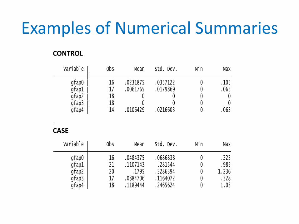
Examples of Numerical Summaries

gfap4 18 .1189444 .2465624 0 1.03 gfap3 17 .0884706 .1164072 0 .328 gfap2 20 .1795 .3286394 0 1.236 gfap1 21 .1107143 .281544 0 .985 gfap0 16 .0484375 .0686838 0 .223 Variable Obs Mean Std. Dev. Min Max

-> pvl = case

gfap4 14 .0106429 .0216603 0 .063 gfap3 18 0 0 0 0 gfap2 18 0 0 0 0 gfap1 17 .0061765 .0179869 0 .065 gfap0 16 .0231875 .0357122 0 .105 Variable Obs Mean Std. Dev. Min Max

-> pvl = controlCONTROL

CASE

Another Way to Visualize 0

.05

.1.1

5.2

.25

.3.3

5.4

.45

.5

0 1 2 3 4 0 1 2 3 4

control case

Mean Visits 95%CI

GFA

P le

vel

time

Mean Response Profiles by PVL StatusMEAN RESPONSE BY CASE/CONTROL STATUS

BIO

MA

RK

ER

0.5

11.5

GF

AP

0 1 2 3 4gfaptime

ID = 58/ID = 186 ID = 70/ID = 205

ID = 76/ID = 212 ID = 90/ID = 213

ID = 96/ID = 240 ID = 98/ID = 250

ID = 107 ID = 126

ID = 138 ID = 154

ID = 158 ID = 159

ID = 174 ID = 183

ID = 185

individual GFAP level change across time among cases

0

.02

.04

.06

.08

.1

GF

AP

0 1 2 3 4gfaptime

ID = 69/ID = 194 ID = 85/ID = 206

ID = 95/ID = 227 ID = 97/ID = 229

ID = 109/ID = 252 ID = 116/ID = 253

ID = 137 ID = 141

ID = 160 ID = 161

ID = 170 ID = 172

ID = 178 ID = 189

ID = 190

individual GFAP level change across time among controls

INDIVIDUAL BIOMARKER LEVEL CHANGE OVER TIME AMONG CASES

INDIVIDUAL BIOMARKER LEVEL CHANGE OVER TIME AMONG CONTROLS

TIME

TIME

BIO

MA

RK

ER

B

IOM

AR

KER

Side-by-Side Box Plot

Males Females

Gfa

p

BIO

MA

RK

ER

Bivariate Data

Dos and Do Nots of Graphing

• Goal of graphing

– To portray data accurately and clearly

• Rules of graphing

– Label and appropriately scale axis

– Simplify, display only the necessary information

– Stay away from pie charts

Take Homes

• Important basic steps in data analyses – Include exploratory data analyses and summary

statistics

• Main rationale for exploratory quantitative data analysis – Get to know your data so that your methods and

inferences will be appropriate

• Statistical tools for inferential statistics – They are vast, we covered just a few