
EPE2013_MagneticTutorial
152
-
Upload
chetan-kotwal -
Category
Documents
-
view
10 -
download
0
description
eee
Transcript of EPE2013_MagneticTutorial


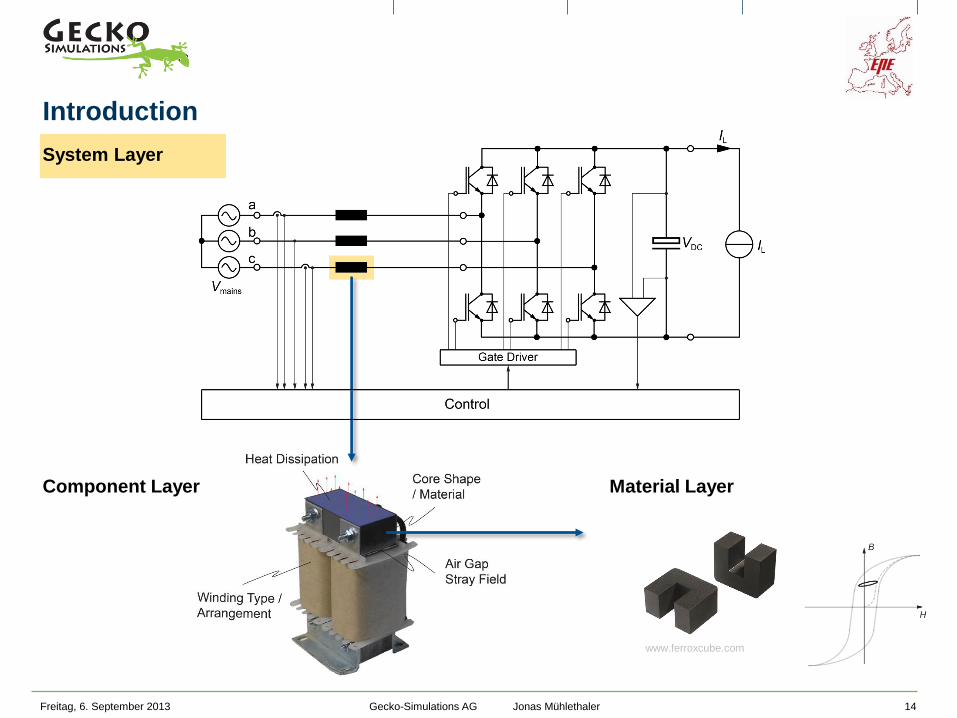
System Layer
Component Layer
Freitag, 6. September 2013 2
Introduction
Gecko-Simulations AG Jonas Mühlethaler

Freitag, 6. September 2013 3
Introduction
Gecko-Simulations AG Jonas Mühlethaler
How are inductors modeled
in GeckoMAGNETICS?

Freitag, 6. September 2013 4
Introduction
System Layer
Component Layer
Material Layer
www.ferroxcube.com
Gecko-Simulations AG Jonas Mühlethaler

Freitag, 6. September 2013 5
Schematic
Modeling Difficulties
- Non-sinusoidal current / flux
waveform
- Current / flux is DC biased
Current / Flux Waveform
Introduction Application of Inductive Components (1) : Buck Converter (DC Current + HF Ripple)
Solutions
- FFT of current waveform for the
calculation of winding losses
- Determine core loss energy for each
segment and for each corner point in the
piecewise-linear flux waveform
- Loss Map enables to consider a DC bias
Gecko-Simulations AG Jonas Mühlethaler

Freitag, 6. September 2013 6
Schematic
Current / Flux Waveform
Introduction Application of Inductive Components (2) : Inductor of DAB Converter (Non-Sinusoidal AC Current)
Modeling Difficulties
- Non-sinusoidal current / flux
waveform
- Core losses occur in the interval of
constant flux
Solutions
- FFT of current waveform for the
calculation of winding losses
- Improved core loss equation that
considers relaxation effects
Gecko-Simulations AG Jonas Mühlethaler

Freitag, 6. September 2013 7
Schematic
Introduction Application of Inductive Components (3) : Three-Phase PFC (Sinusoidal Current + HF Ripple)
Modeling Difficulties
- Non-sinusoidal current / flux
waveform
- Major loop and many (DC biased)
minor loops
Solutions
- FFT of current waveform for the
calculation of winding losses
- Determine core loss energy for each
segment and for each corner point in the
piecewise-linear flux waveform (-> minor
loop losses)
- Add major loop losses
Current / Flux Waveform
Gecko-Simulations AG Jonas Mühlethaler

Freitag, 6. September 2013 8
Introduction Overview About Different Flux Waveforms
Sinusoidal
DC Current +
HF Ripple
Non-Sinusoidal AC
Current
Sinusoidal Current
+ HF Ripple
Major Loop
Minor Loop
Gecko-Simulations AG Jonas Mühlethaler

Freitag, 6. September 2013 9
Introduction
System Layer
Component Layer
Material Layer
www.ferroxcube.com
Gecko-Simulations AG Jonas Mühlethaler

Freitag, 6. September 2013 10
Introduction Overview About Other Modeling Issues
Air Gap
Stray Field
Current
Distribution
Flux Density
Distribution
Heat Dissipation
Core Type
Winding Type /
Arrangement
Gecko-Simulations AG Jonas Mühlethaler
Freitag, 6. September 2013 11
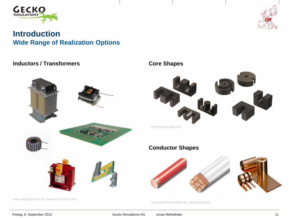
Inductors / Transformers
Conductor Shapes
Core Shapes
Introduction Wide Range of Realization Options
www.ferroxcube.com
www.wagnergrimm.ch, www.ferroxcube.com
www.pack-feindraehte.de, www.jiricek.de
Gecko-Simulations AG Jonas Mühlethaler

Freitag, 6. September 2013 12
1) A reluctance model is introduced to describe the
electric / magnetic interface, i.e. L = f(i).
2) Core losses are calculated.
3) Winding losses are calculated.
4) Inductor temperature is calculated.
Introduction Modeling Inductive Components (1)
Reluctance Model
Procedure
Gecko-Simulations AG Jonas Mühlethaler

Freitag, 6. September 2013 13
The following effects will be taken into consideration:
Magnetic Circuit Model (e.g. for Inductance Calculation):
Air gap stray field
Non-linearity of core material
Core Losses:
DC Bias
Different flux waveforms (link to circuit simulator)
Wide range of flux densities and frequencies
Different core shapes
Winding Losses:
Skin and proximity effect
Stray field proximity effect
Effect of core on magnetic field distribution
Litz, solid, and foil conductors
Introduction Modeling Inductive Components (2)
Gecko-Simulations AG Jonas Mühlethaler
Freitag, 6. September 2013 14
Introduction
System Layer
Component Layer
Material Layer
www.ferroxcube.com
Gecko-Simulations AG Jonas Mühlethaler
Freitag, 6. September 2013 15
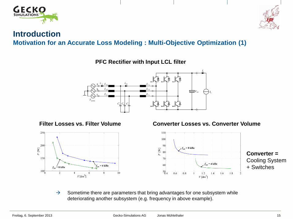
Filter Losses vs. Filter Volume
Sometime there are parameters that bring advantages for one subsystem while
deteriorating another subsystem (e.g. frequency in above example).
Introduction Motivation for an Accurate Loss Modeling : Multi-Objective Optimization (1)
Converter Losses vs. Converter Volume
PFC Rectifier with Input LCL filter
Converter =
Cooling System
+ Switches
Gecko-Simulations AG Jonas Mühlethaler

Freitag, 6. September 2013 16
In order to get an optimal system design, an overall system
optimization has to be performed.
It is (often) not enough to optimize subsystems independent
of each other.
Introduction Motivation for an Accurate Loss Modeling : Multi-Objective Optimization (2)
Losses of a Loss-Optimized Design
Optimal Frequency
6 kHz
Gecko-Simulations AG Jonas Mühlethaler

Outline
Freitag, 6. September 2013 17
Magnetic Circuit Modeling
Core Loss Modeling
Winding Loss Modeling
Thermal Modeling
Multi-Objective Optimization
Summary & Conclusion
Gecko-Simulations AG Jonas Mühlethaler

Freitag, 6. September 2013 18
Electric Network Magnetic Network
Conductivity / Permeability
Resistance / Reluctance
Voltage / MMF
Current / Flux
/ ( )R l A
m / ( )R l A
2
1
d
P
P
V E s 2
1
m d
P
P
V H s
dA
I J A dA
B A
Magnetic Circuit Modeling Reluctance Model
Gecko-Simulations AG Jonas Mühlethaler

Magnetic Circuit Modeling Why a Reluctance Model is Needed
Freitag, 6. September 2013 19
calculate the inductance ( L = N2/Rtot )
calculation the saturation current
calculate the air gap stray field
calculate the core flux density
A reluctance model is needed in order to
Gecko-Simulations AG Jonas Mühlethaler
Accurate loss modeling!

Freitag, 6. September 2013 20
Reluctance Calculation
m
0 r
i
i
lR
A
Magnetic Circuit Modeling Core Reluctance
Core Reluctance Dimensions
Mean magnetic
length Mean magnetic
cross-sectional
area
Gecko-Simulations AG Jonas Mühlethaler

Magnetic Circuit Modeling Air Gap Reluctance : Different Approaches (1)
Freitag, 6. September 2013 21
g
m
0 g
lR
A
Assumption of Homogeneous Field Distribution
gl
gA
Air gap length
Air gap cross-sectional area
g
m
0 g g( )( )
lR
a l t l
e.g. [1] (for a cross section with dimension a x t):
[1] N. Mohan, T. M. Undeland, and W. P. Robbins - “Power
Electronics – Converter, Applications, and Design”,
John Wiley & Sons, Inc., 2003
Increase of the Air Gap Cross-Sectional Area
a
a
a
lg
Gecko-Simulations AG Jonas Mühlethaler

Freitag, 6. September 2013 22
Schwarz-Christoffel Transformation
Magnetic Circuit Modeling Air Gap Reluctance : Different Approaches (2)
[2] K. J. Binns, P. J. Lawrenson, and C. W. Trowbridge, «The Analytical and Numerical Solution of Electric
and Magnetic Fields», John Wiley & Sons, Inc., 1992
( ) 2 ln 1 1 ln 2 1l
z t t t t
(z and t are complex numbers)
( ) lnV
v t t
Transformation Equation z(t) Transformation Equation v(t)
Gecko-Simulations AG Jonas Mühlethaler

Freitag, 6. September 2013 23
Solution to 2-D problems found in literature, e.g. in [3]
Some 3-D solution to problem found in literature; however, they are complex [4] and/or
limited to one air gape shape [5]
Can’t be directly applied to 3-D problems.
More simple and universal model desired.
[3] A. Balakrishnan, W. T. Joines, and T. G. Wilson - “Air-gap reluctance and inductance calculations for
magnetic circuits using a Schwarz-Christoffel transformation”, IEEE Transaction on Power Electronics,
vol. 12, pp. 654—663, July 1997.
[4] P. Wallmeier, “Automatisierte Optimierung von induktiven Bauelementen für Stromrichteranwendungen”,
PhD Thesis, Universität – Gesamthochschule Paderborn, 2001.
[5] E. C. Snelling, “Soft Ferrites - Properties and Applications”, 2nd edition, Butterworths, 1988
Magnetic Circuit Modeling Air Gap Reluctance : Different Approaches (3)
Gecko-Simulations AG Jonas Mühlethaler

Magnetic Circuit Modeling Aim of New Model
Freitag, 6. September 2013 24
Illustration of Different Air Gap Shapes:
Air gap reluctance calculation that
- considers the three dimensionality,
- is reasonable easy-to-handle,
- is capable of modeling different shapes of air gaps,
- while still achieving a high accuracy.
Gecko-Simulations AG Jonas Mühlethaler
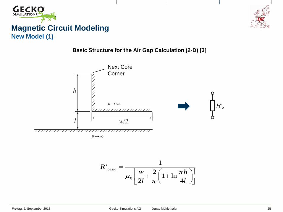
Freitag, 6. September 2013 25
basic
0
1'
21 ln
2 4
Rw h
l l
Basic Structure for the Air Gap Calculation (2-D) [3]
Magnetic Circuit Modeling New Model (1)
Next Core
Corner
Gecko-Simulations AG Jonas Mühlethaler
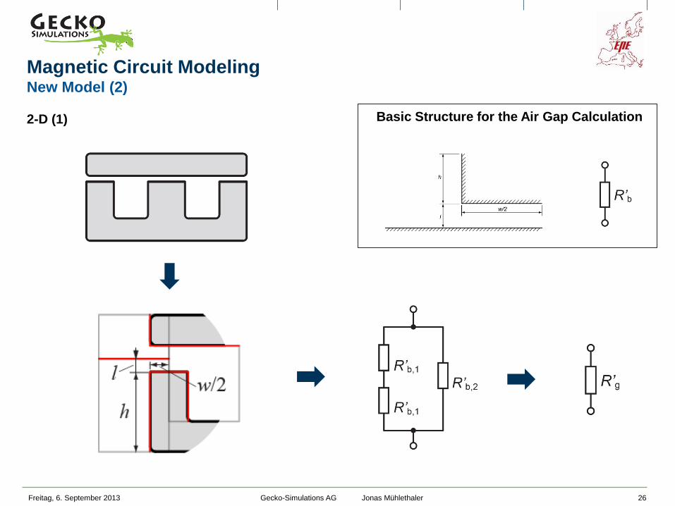
Magnetic Circuit Modeling New Model (2)
Freitag, 6. September 2013 26
2-D (1)
Basic Structure for the Air Gap Calculation
Gecko-Simulations AG Jonas Mühlethaler

Basic Structure for the Air Gap Calculation
Freitag, 6. September 2013 27
Air Gap Type 1
Air Gap Type 2
Air Gap Type 3
Magnetic Circuit Modeling New Model (3)
2-D (2)
basic
0
1'
21 ln
2 4
Rw h
l l
Gecko-Simulations AG Jonas Mühlethaler
Freitag, 6. September 2013 28
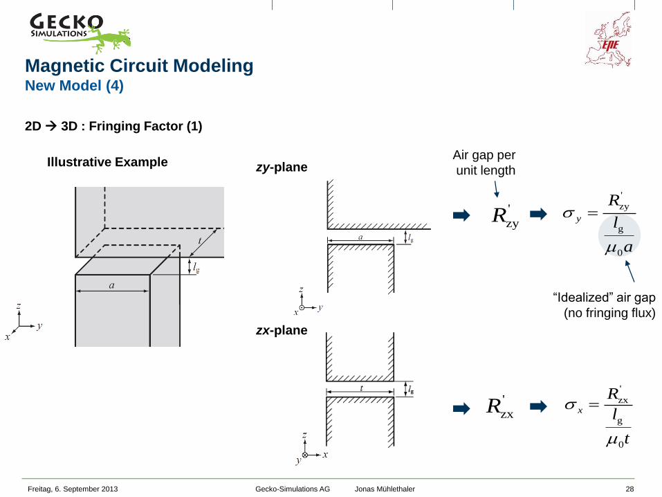
2D 3D : Fringing Factor (1)
Illustrative Example zy-plane
zx-plane
'
zyR
Magnetic Circuit Modeling New Model (4)
'
zy
g
0
y
R
l
a
“Idealized” air gap
(no fringing flux)
'
zx
g
0
x
R
l
t
Air gap per
unit length
'
zxR
Gecko-Simulations AG Jonas Mühlethaler

Freitag, 6. September 2013 29
Illustrative Example
3-D Fringing Factor:
“Idealized” air gap
(no fringing flux)
g
g
0
lR
at
2D 3D : Fringing Factor (2)
Magnetic Circuit Modeling New Model (5)
x y
Alternative Interpretation:
Increase of air gap cross sectional area
1
x
A A’ A’’
1
y
[6] J. Mühlethaler, J.W. Kolar, and A. Ecklebe, “A Novel Approach for 3D Air Gap Reluctance Calculations”,
in Proc. of the ICPE - ECCE Asia, Jeju, Korea, 2011
Gecko-Simulations AG Jonas Mühlethaler

Freitag, 6. September 2013 30
a = 40 mm; h = 40 mm
3-D FEM Simulation
Modeled Example Results
Magnetic Circuit Modeling FEM Results
Gecko-Simulations AG Jonas Mühlethaler

Freitag, 6. September 2013 31
Inductance Calculation
EPCOS E55/28/21, N = 80
Magnetic Circuit Modeling Experimental Results
Saturation Calculation
EPCOS E55/28/21, N = 80,
lg = 1 mm, Bsat = 0.45 T
Measurement
Isat = 3.7 A
Gecko-Simulations AG Jonas Mühlethaler

Freitag, 6. September 2013 32
∅ = 𝑓(𝑅m(∅), 𝐼) = 𝑓(∅, 𝐼) 𝑅m = 𝑓(∅)
𝐿 =𝑁2
𝑅tot(𝐼)
Flux and Reluctance Calculation
∅ = 𝑓(𝑅m(∅), 𝐼)
Magnetic Circuit Modeling Non-Linearity of the Core Material
Reluctance Model
0 50 100 150 200
0.58
0.6
0.62
0.64
0.66
0.68
0.7
0.72
0.74Inductance
Inducta
nce [
mL]
Current [A]
1234567891011121314
15
16
17
18
19
20
21
0 500 10000
0.5
1
1.5
1
2
3
4
5
6
7
8
9
10
11
12
13
14 15 16 17 18 19 20 21
B-H Relation
Magentic F
lux D
ensity [
T]
Magnetic Field [A/m]
This equation must be solved iteratively by
using a numerical solving method, e.g. the
Newton’s method.
Inductance Calculation
Gecko-Simulations AG Jonas Mühlethaler

Freitag, 6. September 2013 33
Aim
Design PFC rectifier system.
Show trade-off between losses and volume.
Illustrative example.
Modeling of boost inductors (three individual inductors L2a = L2b = L2c) will
be step-by-step illustrated in the course of this presentation.
Example Introduction
Schematic
Gecko-Simulations AG Jonas Mühlethaler

Freitag, 6. September 2013 34
Example Reluctance Model (1)
c1
0 r0 r
00
(2 )2 82
(2 )
2
(2 20mm)60mm 2 20mm A82 3654
(2 20mm)20 '000 20mm 28mm Vs20 '000 28mm
2
ado a
Raat
t
Material
Grain-oriented steel (M165-35S)
Calculation of Core Reluctances
Reluctance Model
c2
0 r0 r
00
(2 )2 2 82
(2 )
2
(2 20mm)60mm 2 20mm + 2 h A82 12184
(2 20mm)20 '000 20mm 28mm Vs20 '000 28mm
2
ado a b
Raat
t
Photo & Dimensions
Gecko-Simulations AG Jonas Mühlethaler

'
zy,2
0g g
1
2 ( )1 ln
2 42 2
R
a b a
l l
Freitag, 6. September 2013 35
Example Reluctance Model (2)
Photo & Dimensions
Material
Grain-oriented steel (M165-35S)
Calculation Air Gap Reluctances
zy-plane
zx-plane
'
zy,1
0g g
1
21 ln
2 42 2
R
a a
l l
'
zy
g
0
0.72y
R
l
a
'
zy,3
0
g g
1
21 ln
2 4
Ra b
l l
Basic Reluctance
'
zx,1
0g g
1
21 ln
2 42 2
R
t a
l l
'
zx
g
0
0.84x
R
l
t
g
g
0
MA1.66
Wbx y
lR
at
Inductance
2
c1 c2 g1 g2
2.66mHN
LR R R R
meas.
2.69 mH
basic
0
1'
21 ln
2 4
Rw h
l l
' ' '
zy,1 zy,2 zy,3'
zy ' ' '
zy,1 zy,2 zy,3
R R RR
R R R
'
zx,2
0g g
1
2 ( )1 ln
2 42 2
R
t b a
l l
' '
zx,1 zx,2'
zx2
R RR
Gecko-Simulations AG Jonas Mühlethaler

Outline
Freitag, 6. September 2013 36
Magnetic Circuit Modeling
Core Loss Modeling
Winding Loss Modeling
Thermal Modeling
Multi-Objective Optimization
Summary & Conclusion
Gecko-Simulations AG Jonas Mühlethaler
Freitag, 6. September 2013 37
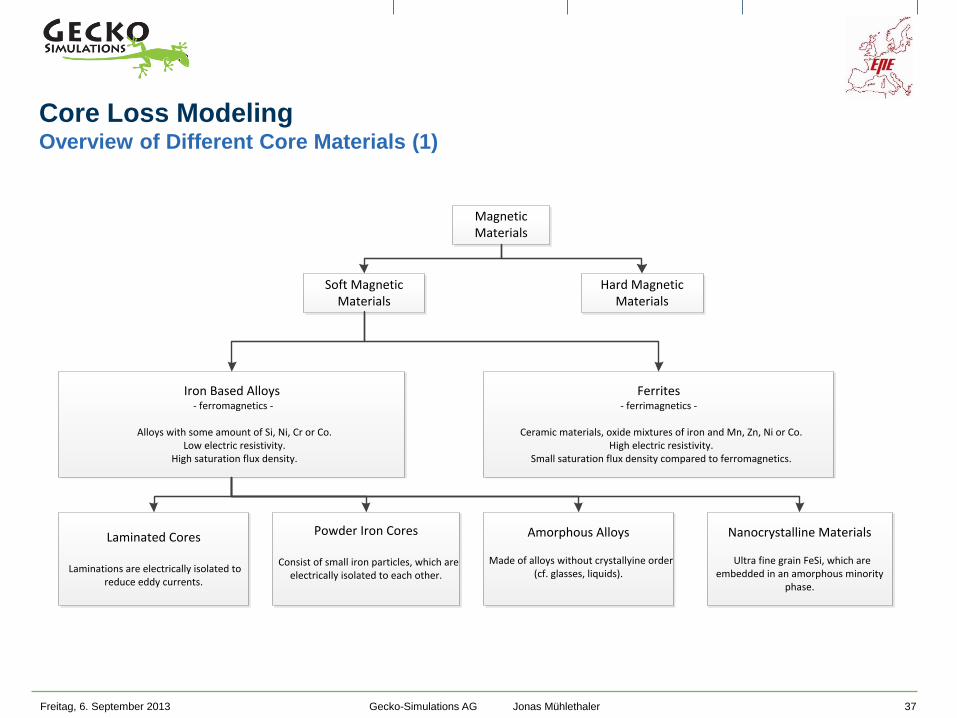
Core Loss Modeling Overview of Different Core Materials (1)
Iron Based Alloys - ferromagnetics -
Alloys with some amount of Si, Ni, Cr or Co. Low electric resistivity.
High saturation flux density.
Ferrites- ferrimagnetics -
Ceramic materials, oxide mixtures of iron and Mn, Zn, Ni or Co. High electric resistivity.
Small saturation flux density compared to ferromagnetics.
Laminated Cores
Laminations are electrically isolated to reduce eddy currents.
Powder Iron Cores
Consist of small iron particles, which are electrically isolated to each other.
Amorphous Alloys
Made of alloys without crystallyine order (cf. glasses, liquids).
Nanocrystalline Materials
Ultra fine grain FeSi, which are embedded in an amorphous minority
phase.
Magnetic Materials
Soft Magnetic Materials
Hard Magnetic Materials
Gecko-Simulations AG Jonas Mühlethaler
Freitag, 6. September 2013 38
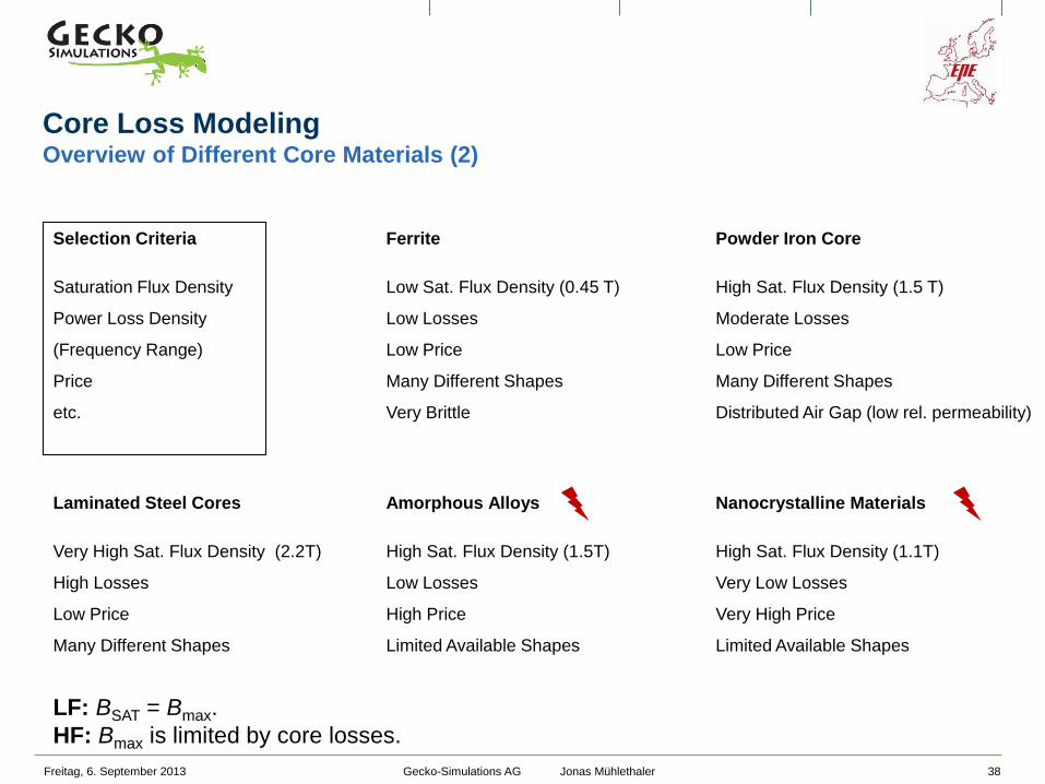
Core Loss Modeling Overview of Different Core Materials (2)
Amorphous Alloys
High Sat. Flux Density (1.5T)
Low Losses
High Price
Limited Available Shapes
Nanocrystalline Materials
High Sat. Flux Density (1.1T)
Very Low Losses
Very High Price
Limited Available Shapes
Laminated Steel Cores
Very High Sat. Flux Density (2.2T)
High Losses
Low Price
Many Different Shapes
Ferrite
Low Sat. Flux Density (0.45 T)
Low Losses
Low Price
Many Different Shapes
Very Brittle
Powder Iron Core
High Sat. Flux Density (1.5 T)
Moderate Losses
Low Price
Many Different Shapes
Distributed Air Gap (low rel. permeability)
Selection Criteria
Saturation Flux Density
Power Loss Density
(Frequency Range)
Price
etc.
LF: BSAT = Bmax.
HF: Bmax is limited by core losses.
Gecko-Simulations AG Jonas Mühlethaler
Freitag, 6. September 2013 39
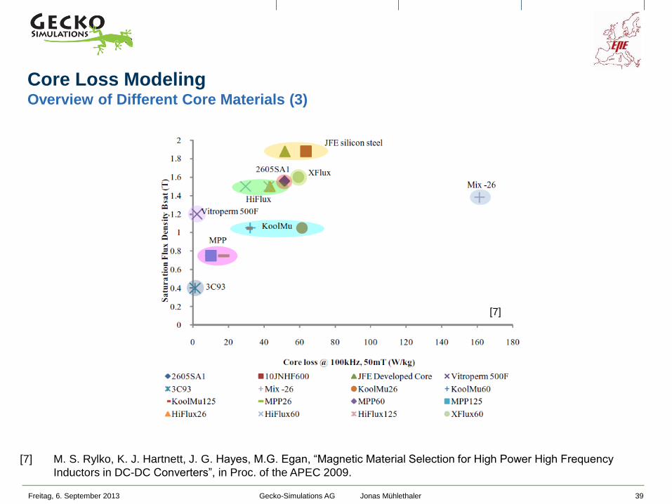
Core Loss Modeling Overview of Different Core Materials (3)
[7] M. S. Rylko, K. J. Hartnett, J. G. Hayes, M.G. Egan, “Magnetic Material Selection for High Power High Frequency
Inductors in DC-DC Converters”, in Proc. of the APEC 2009.
[7]
Gecko-Simulations AG Jonas Mühlethaler

Freitag, 6. September 2013 40
Core Loss Modeling Physical Origin of Core Losses (1)
B-H-Loop
Weiss Domains / Domain Walls
- Spontaneous magnetization.
- Material is divided to saturated domains
(Weiss domains).
- In case an external field is applied, the
domain walls are shifted or the magnetic
moments within the domains change their
direction. The net magnetization becomes
greater than zero.
- The flux change is partly irreversible, i.e.
energy is dissipated as heat.
- The reason for this are the so called
Barkhausen jumps, that lead to local eddy
current losses.
- In case the loop is traversed very slowly,
these Barkhausen jumps lead to the static
hysteresis losses.
Gecko-Simulations AG Jonas Mühlethaler

Freitag, 6. September 2013 41
Core Loss Modeling Physical Origin of Core Losses (2)
B-H-Loop
- If the process would be fully reversible,
going from B1 to B2 would store potential
energy in the magnetic material that is later
released (i.e. the area of the closed loop
would be zero).
- Since the process is partly irreversible, the
area of the closed loop represents the
energy loss per cycle
Gecko-Simulations AG Jonas Mühlethaler
𝑊 = 𝐻d𝐵

Freitag, 6. September 2013 42
(Static) hysteresis loss
Rate-independent BH Loop.
Loss energy per cycle is constant.
Irreversible changes each within a small
region of the lattice (Barkhausen jumps).
These rapid, irreversible changes are
produced by relatively strong local fields within
the material.
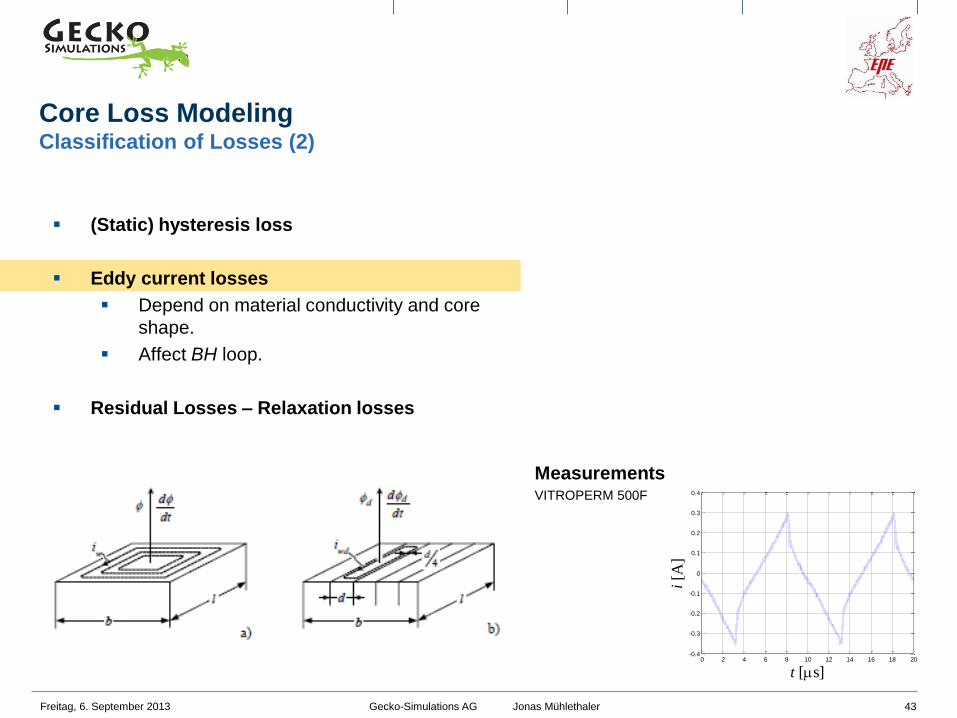
Eddy current losses
Residual Losses – Relaxation losses
Core Loss Modeling Classification of Losses (1)
Gecko-Simulations AG Jonas Mühlethaler
Freitag, 6. September 2013 43
(Static) hysteresis loss
Eddy current losses
Depend on material conductivity and core
shape.
Affect BH loop.
Residual Losses – Relaxation losses
Measurements VITROPERM 500F
0 2 4 6 8 10 12 14 16 18 20-0.4
-0.3
-0.2
-0.1
0
0.1
0.2
0.3
0.4
i [A
]t [s]
Core Loss Modeling Classification of Losses (2)
Gecko-Simulations AG Jonas Mühlethaler

Freitag, 6. September 2013 44
(Static) hysteresis loss
Eddy current losses
Residual losses – Relaxation losses
Rate-dependent BH Loop.
Reestablishment of a thermal equilibrium is
governed by relaxation processes.
Restricted domain wall motion.
Core Loss Modeling Classification of Losses (3)
Gecko-Simulations AG Jonas Mühlethaler

Freitag, 6. September 2013 45
Sinusoidal
Core Loss Modeling Typical Flux Waveforms
Triangular
Trapezoidal
Combination
e.g. boost inductor of Dual Active
Bridge
e.g. Boost inductor in PFC
e.g. Buck / Boost converter
e.g. 50/60 Hz isolation transformer
Gecko-Simulations AG Jonas Mühlethaler

Freitag, 6. September 2013 46
Steinmetz Approach
Core Loss Modeling Outline of Different Modeling Approaches
- Simple
- Steinmetz parameter
are valid only in a
limited flux density
and frequency range
- DC Bias not
considered
- (Only for sinusoidal
flux waveforms)
Loss Map Approach
Loss Separation Hysteresis Model
α βP k f B
hyst eddy residualP P P P (e.g. Preisach Model, Jiles-Atherton
Model)
(Loss Database)
- Needed parameters often unknown
- Model is widely applicable
- Increases physical understanding of loss
mechanisms
- Measuring core losses is
indispensable to overcome limits of
Steinmetz approach
- Difficult to parameterize
- Increases physical understanding of loss
mechanisms
ww
ww
.epcos.c
om
Gecko-Simulations AG Jonas Mühlethaler

Core Loss Modeling Overview of Hybrid Modeling Approach
Freitag, 6. September 2013 47
Loss Map
(Loss Material Database)
n
l
ll
T
i PQtBt
Bk
TP
1
rr
0
v dd
d1
r r r, , , , , , ,ik k q
P
V
Outline of Discussion
- Derivation of the
i2GSE. (1)
- How to measure core
losses in order to
build loss map. (2)
- Use of loss map. (3)
- How to calculate core
losses for cores of
different shapes? (4)
(1)
(2)/(3)
(4)
“The best of both worlds” (Steinmetz & Loss Map approach)
Gecko-Simulations AG Jonas Mühlethaler

Steinmetz Equation SE
- Only sinusoidal waveforms ( iGSE).
α β
vˆP k f B
Freitag, 6. September 2013 48
iGSE
- DC bias not considered
- Relaxation effect not considered ( i2GSE)
- Steinmetz parameter are valid only for a limited flux density and
frequency range
21
0(2 ) cos 2 d
i
kk
Core Loss Modeling Derivation of the i2GSE – Motivation (1)
v
0
1 dd
d
T
i
BP k B t
T t
Pv : time-average
power loss per
unit volume
Gecko-Simulations AG Jonas Mühlethaler

Freitag, 6. September 2013 49
iGSE [8]
21
0(2 ) cos 2 d
i
kk
Core Loss Modeling Derivation of the i2GSE – Motivation (2)
v
0
1 dd
d
T
i
BP k B t
T t
[8] K. Venkatachalam, C. R. Sullivan, T. Abdallah, and H. Tacca, “Accurate prediction of ferrite core loss with nonsinusoidal
waveforms using only Steinmetz parameters”, in Proc. of IEEE Workshop on Computers in Power Electronics, pp. 36-41, 2002.
Idea
- Generalized formula that is applicable for
different flux waveforms
- Losses depend on dB/dt
For Sinusoidal Waveforms
How to apply the formula?
v
0
1 dd
d 2
T
i
B BP k B t kf
T t
v (1 ) ...(1 )
ik B BP DT B D T B
T DT D T
Gecko-Simulations AG Jonas Mühlethaler

Freitag, 6. September 2013 50
Waveform
v
0
1 dd
d
T
i
BP k B t
T t
iGSE
Core Loss Modeling Derivation of the i2GSE – Motivation (3)
Results
Conclusion
Losses in the phase of constant flux!
Gecko-Simulations AG Jonas Mühlethaler

Freitag, 6. September 2013 51
Relaxation Losses
Rate-dependent BH Loop.
Reestablishment of a thermal
equilibrium is governed by
relaxation processes.
Restricted domain wall motion.
Core Loss Modeling Derivation of the i2GSE – B-H-Loop
Current Waveform
Gecko-Simulations AG Jonas Mühlethaler

Freitag, 6. September 2013 52
Derivation (1)
Relaxation loss energy can be described with
is independent of operating point.
How to determine E?
Waveform
Loss Energy per Cycle
1
e1
t
EE
Core Loss Modeling Derivation of the i2GSE – Model Derivation 1 (1)
Gecko-Simulations AG Jonas Mühlethaler

Freitag, 6. September 2013 53
Waveform
r
r
)(d
dr
BtBt
kE
E – Measurements
Conclusion
E follows a power
function!
Core Loss Modeling Derivation of the i2GSE – Model Derivation 1 (2)
Gecko-Simulations AG Jonas Mühlethaler

Freitag, 6. September 2013 54
Model Part 1
n
l
l
T
i PtBt
Bk
TP
1
r
0
v dd
d1
1
r
r
e1)(d
d1rr
t
l BtBt
kT
P
Core Loss Modeling Derivation of the i2GSE – Model Derivation 1 (3)
Gecko-Simulations AG Jonas Mühlethaler

Freitag, 6. September 2013 55
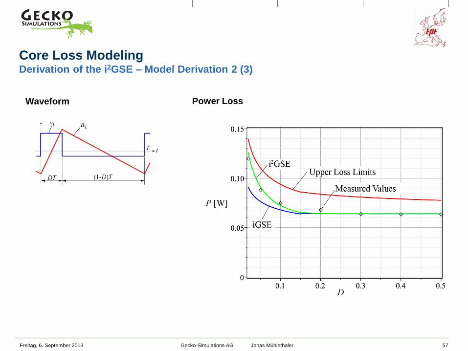
Explanation
1) For values of D close to 0 or close to 1 a loss underestimation is expected when calculating losses with iGSE (no
relaxation losses included).
2) For values of D close to 0.5 the iGSE is expected to be accurate.
3) Adding the relaxation term leads to the upper loss limit, while the iGSE represents the lower loss limit.
4) Losses are expected to be in between the two limits, as has been confirmed with measurements.
Waveform
Power Loss
Core Loss Modeling Derivation of the i2GSE – Model Derivation 2 (1)
Gecko-Simulations AG Jonas Mühlethaler

Freitag, 6. September 2013 56
Model Adaption
Qrl should be 1 for D = 0
Qrl should be 0 for D = 0.5
Qrl should be such that calculation fits a triangular
waveform measurement.
Waveform
Power Loss
n
l
ll
T
i PQtBt
Bk
TP
1
rr
0
v dd
d1
D
Dq
ttB
ttBq
lQ 1d/)(d
d/)(d
r
rr
ee
Core Loss Modeling Derivation of the i2GSE – Model Derivation 2 (2)
Gecko-Simulations AG Jonas Mühlethaler
Freitag, 6. September 2013 57
Waveform
Power Loss
Core Loss Modeling Derivation of the i2GSE – Model Derivation 2 (3)
Gecko-Simulations AG Jonas Mühlethaler
Freitag, 6. September 2013 58
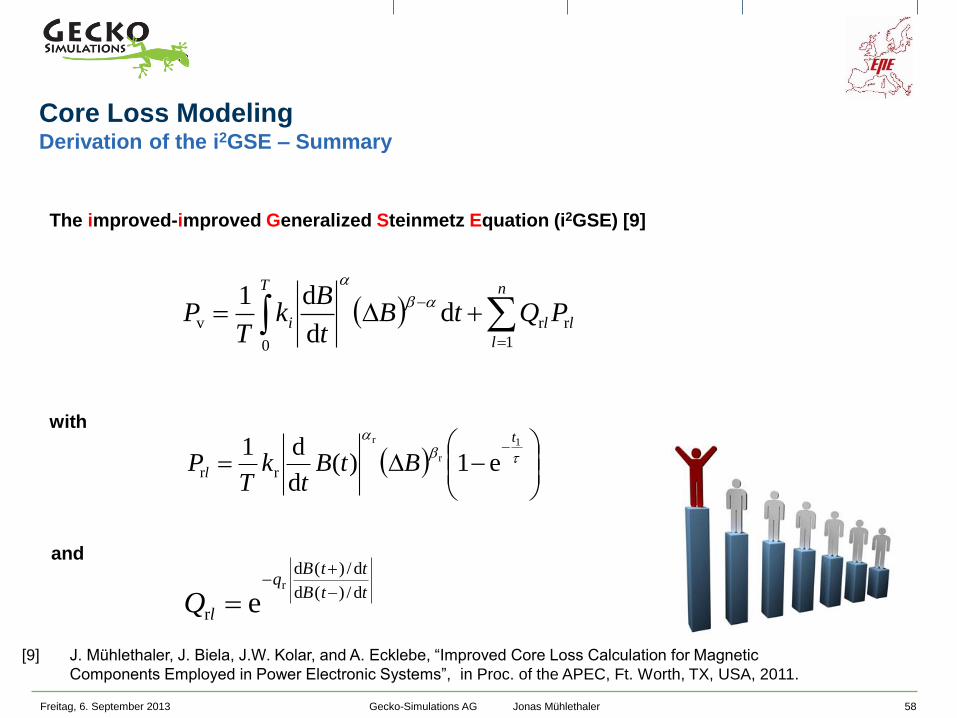
The improved-improved Generalized Steinmetz Equation (i2GSE) [9]
n
l
ll
T
i PQtBt
Bk
TP
1
rr
0
v dd
d1
ttB
ttBq
lQd/)(d
d/)(d
r
r
e
1
r
r
e1)(d
d1rr
t
l BtBt
kT
P
with
and
Core Loss Modeling Derivation of the i2GSE – Summary
[9] J. Mühlethaler, J. Biela, J.W. Kolar, and A. Ecklebe, “Improved Core Loss Calculation for Magnetic
Components Employed in Power Electronic Systems”, in Proc. of the APEC, Ft. Worth, TX, USA, 2011.
Gecko-Simulations AG Jonas Mühlethaler

Freitag, 6. September 2013 59
i2GSE
for 0 and 22
0 for 2 and 2d
dfor 2 and
2
0 for and
Bt t T t
T t
t T t t TB
Btt T t T t
T t
t T t t T
Core Loss Modeling Derivation of the i2GSE – Example
Evaluated for each piecewise-linear flux
segment
Evaluated for each voltage step, i.e. for each
corner point in a piecewise-linear flux
waveform.
Example
n
l
ll
T
i PQtBt
Bk
TP
1
rr
0
v dd
d1
2
v r r
1
2
2i l l
l
T t BP k B Q P
T T t
Qr1 = Qr2 = 0
r
r
r1 r2 r
11 e
2
tB
P P k BT T t
with
Gecko-Simulations AG Jonas Mühlethaler

Freitag, 6. September 2013 60
Remaining Problems
Steinmetz parameter are valid only in a limited flux density and frequency range.
Core Losses vary under DC bias condition.
Modeling relaxation and DC bias effects need parameters that are not given by core material
manufacturers.
i2GSE
n
l
ll
T
i PQtBt
Bk
TP
1
rr
0
v dd
d1
Measuring core losses is indispensable!
Core Loss Modeling Derivation of the i2GSE – Conclusion
Evaluated for each piecewise-linear flux
segment
Evaluated for each voltage step, i.e. for each
corner point in a piecewise-linear flux
waveform.
Gecko-Simulations AG Jonas Mühlethaler

Core Loss Modeling Overview of Hybrid Modeling Approach
Freitag, 6. September 2013 61
Loss Map
(Loss Material Database)
n
l
ll
T
i PQtBt
Bk
TP
1
rr
0
v dd
d1
r r r, , , , , , ,ik k q
P
V
Outline of Discussion
- Derivation of the
i2GSE. (1)
- How to measure core
losses in order to
build loss map. (2)
- Use of loss map. (3)
- How to calculate core
losses for cores of
different shapes? (4)
(1)
(2)/(3)
(4)
“The best of both worlds” (Steinmetz & Loss Map approach)
Gecko-Simulations AG Jonas Mühlethaler

Freitag, 6. September 2013 62
2 e 0
1( ) ( ) d
t
B t uN A
1
e
( )( )
N i tH t
l
3
[
]
]
[
P W
V m
Core Loss Modeling Core Loss Measurement – Measurement Principle
Voltage 0 … 450 V
Current 0 … 25 A
Frequency 0 … 200 kHz
Excitation System
Loss Extraction
Schematic Waveforms
Sinusoidal
Triangular
Trapezoidal
Gecko-Simulations AG Jonas Mühlethaler
= 𝑓 𝐻d𝐵
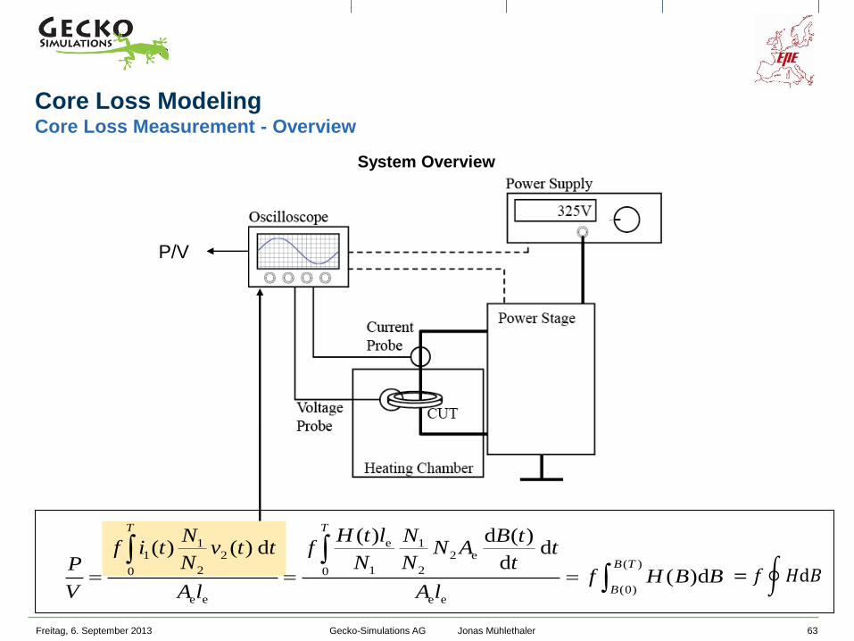
Core Loss Modeling Core Loss Measurement - Overview
Freitag, 6. September 2013 63
System Overview
P/V
e1 11 2 2 e
( )2 1 20 0
(0)e e e e
( ) d ( )( ) ( ) d d
d( )d
T T
B T
B
H t lN N B tf i t v t t f N A t
N N N tPf H B B
V A l A l
Gecko-Simulations AG Jonas Mühlethaler
= 𝑓 𝐻d𝐵

Core Loss Modeling Overview of Hybrid Modeling Approach
Freitag, 6. September 2013 64
Loss Map
(Loss Material Database)
n
l
ll
T
i PQtBt
Bk
TP
1
rr
0
v dd
d1
r r r, , , , , , ,ik k q
P
V
Outline of Discussion
- Derivation of the
i2GSE. (1)
- How to measure core
losses in order to
build loss map. (2)
- Use of loss map. (3)
- How to calculate core
losses for cores of
different shapes? (4)
(1)
(2)/(3)
(4)
“The best of both worlds” (Steinmetz & Loss Map approach)
Gecko-Simulations AG Jonas Mühlethaler

Freitag, 6. September 2013 65
Core Loss Modeling Needed Loss Map Structure
Content of Loss Map Typical flux waveform
Gecko-Simulations AG Jonas Mühlethaler

Freitag, 6. September 2013 66
Core Loss Modeling Minor and Major Loops
Idea
Major Loop
Minor Loop
Losses due to Minor and Major
Loops are calculated independent
of each other and summed up.
Implementation
Major
P
V
Piecewise Linear Segment (+ Turning Point)
P
V
Piecewise Linear Major
Segment (+ Turning Point)
P P P
V V V
Actually, it is not considered how
the minor loop closes: each
piecewise linear segment is
modeled as having half the losses
of its corresponding closed loop
(cf. next slides).
Gecko-Simulations AG Jonas Mühlethaler

Freitag, 6. September 2013 67
(I)
(II)
Core Loss Modeling Hybrid Loss Modeling Approach (1)
HDC / BDC
Gecko-Simulations AG Jonas Mühlethaler

Freitag, 6. September 2013 68
Loss Map
n
l
ll
T
i PQtBt
Bk
TP
1
rr
0
v dd
d1
P
V
Core Loss Modeling Hybrid Loss Modeling Approach (2)
(I)
(II)
These equations arise when one evaluates the
i2GSE for symmetric triangular waveforms.
Three loss map
operating points
are required in
order to extract
the parameters ,
, and k (or ki).
Evaluated for the according piecewise-
linear flux segment
Evaluated for the according corner point
in a piecewise-linear flux waveform.
v1 1 1
v2 2 2
v3 3 3
2
2
2
i
i
i
P k f B
P k f B
P k f B
Gecko-Simulations AG Jonas Mühlethaler

Freitag, 6. September 2013 69
Interpolation and Extrapolation
(HDC*, T*, B*, f*)
HDC and T
B and f
Core Loss Modeling Hybrid Loss Modeling Approach (3)
Gecko-Simulations AG Jonas Mühlethaler

Freitag, 6. September 2013 70
Advantages of Hybrid Approach (Loss Map and i2GSE):
Relaxation effects are considered (i2GSE).
A good interpolation and extrapolation between premeasured operating points is achieved.
Loss map provides accurate i2GSE parameters for a wide frequency and flux density range.
A DC bias is considered as the loss map stores premeasured operating points at different DC
bias levels.
Core Loss Modeling Hybrid Loss Modeling Approach (4)
Gecko-Simulations AG Jonas Mühlethaler

Freitag, 6. September 2013 71
Core Losses Summary of Loss Density Calculation
Sinusoidal
Triangular
Trapezoidal
α βP k f B
n
l
ll
T
i PQtBt
Bk
TP
1
rr
0
v dd
d1
with Q 0, n = 1
n
l
ll
T
i PQtBt
Bk
TP
1
rr
0
v dd
d1
with Q = 1, n = 2
n
l
ll
T
i PQtBt
Bk
TP
1
rr
0
v dd
d1
with different Q’s and n >> 0.
Combination
Gecko-Simulations AG Jonas Mühlethaler

Core Loss Modeling Overview of Hybrid Modeling Approach
Freitag, 6. September 2013 72
Loss Map
(Loss Material Database)
n
l
ll
T
i PQtBt
Bk
TP
1
rr
0
v dd
d1
r r r, , , , , , ,ik k q
P
V
Outline of Discussion
- Derivation of the
i2GSE. (1)
- How to measure core
losses in order to
build loss map. (2)
- Use of loss map. (3)
- How to calculate core
losses for cores of
different shapes? (4)
(1)
(2)/(3)
(4)
“The best of both worlds” (Steinmetz & Loss Map approach)
Gecko-Simulations AG Jonas Mühlethaler

Freitag, 6. September 2013 73
1) The flux density in every core section of
(approximately) homogenous flux density
is calculated.
2) The losses of each section are calculated.
3) The core losses of each section are then
summed-up to obtain the total core
losses.
Reluctance Model
Procedure
Core Loss Modeling Effect of Core Shape
∅ = 𝑓(𝑅m(∅), 𝐼) = 𝑓(∅, 𝐼)
Gecko-Simulations AG Jonas Mühlethaler

Motivation for Effective Core Dimensions
Core loss densities are needed to model core
losses. It is difficult to determine these loss
densities from a toroid, since the flux density is not
distributed homogeneously in a toroid.
Freitag, 6. September 2013 74
2
2 1e
1 2
ln /
1/ 1/
h r rA
r r
2 1e
1 2
2 ln /
1/ 1/
r rl
r r
Core Loss Modeling Effective Core Dimensions of Toroid
Illustration
Effective magnetic cross-section
Effective magnetic length
Idea for Real Toroid
Find effective core magnetic length and cross
section, so one can calculate as if it were an ideal
toroid, i.e. as if the flux density distribution were
homogenous.
Definition: Ideal Toroid
A toroid is ideal when he has a homogenous flux
density distribution over the radius (r1 r2).
Gecko-Simulations AG Jonas Mühlethaler

Freitag, 6. September 2013 75
Eddy current loss density can be determined as [5]
Core Loss Modeling Impact of Core Shape on Eddy Current Losses
2
eddy
ec
ˆ( )BfdP
k
For a laminated core it is
2
eddy
ˆ( )
6
BfdP
The eddy current losses per unit volume depend not on the shape of the bulk material, but on
the size and geometry of the insulated regions.
In case of laminated iron cores, it is still appropriate to calculate with core loss densities that
have been measured on a sample core with a geometrically different bulk material, but with the
same lamination or tape thickness.
[5] E. C. Snelling, “Soft Ferrites - Properties and Applications”, 2nd edition, Butterworths, 1988
Gecko-Simulations AG Jonas Mühlethaler

Freitag, 6. September 2013 76
Losses in gapped tape wound cores higher than expected!
www.vacuumschmelze.de
Core Loss Modeling Effect in Tape Wound Cores
Thin ribbons (approx. 20m)
Wound as toroid or as double C core.
Amorphous or nanocrystalline materials.
Gecko-Simulations AG Jonas Mühlethaler

Freitag, 6. September 2013 77
Machining process
Surface short circuits introduced by machining
(particular a problem in in-house production).
After treatment may reduce this effect. At ETH, a core was put in an 40% ferric chloride FeCl3
solution after cutting, which substantially (more than 50%) decreased the core losses.
Core Loss Modeling Effect in Tape Wound Cores - Cause 1 : Interlamination Short Circuits
Gecko-Simulations AG Jonas Mühlethaler

Freitag, 6. September 2013 78
Core Loss Modeling Effect in Tape Wound Cores - Cause 2 : Orthogonal Flux Lines (1)
Fringing
flux
Main flux
Eddy current
Eddy current
A flux orthogonal to the ribbons leads to very high eddy current losses!
Gecko-Simulations AG Jonas Mühlethaler

Freitag, 6. September 2013 79
Horizontal Displacement
Vertical Displacement
An experiment that illustrates well the loss increase due to an orthogonal flux is given here.
Core Loss Modeling Effect in Tape Wound Cores - Cause 2 : Orthogonal Flux Lines (2)
Core Loss Results
Displacements
Gecko-Simulations AG Jonas Mühlethaler
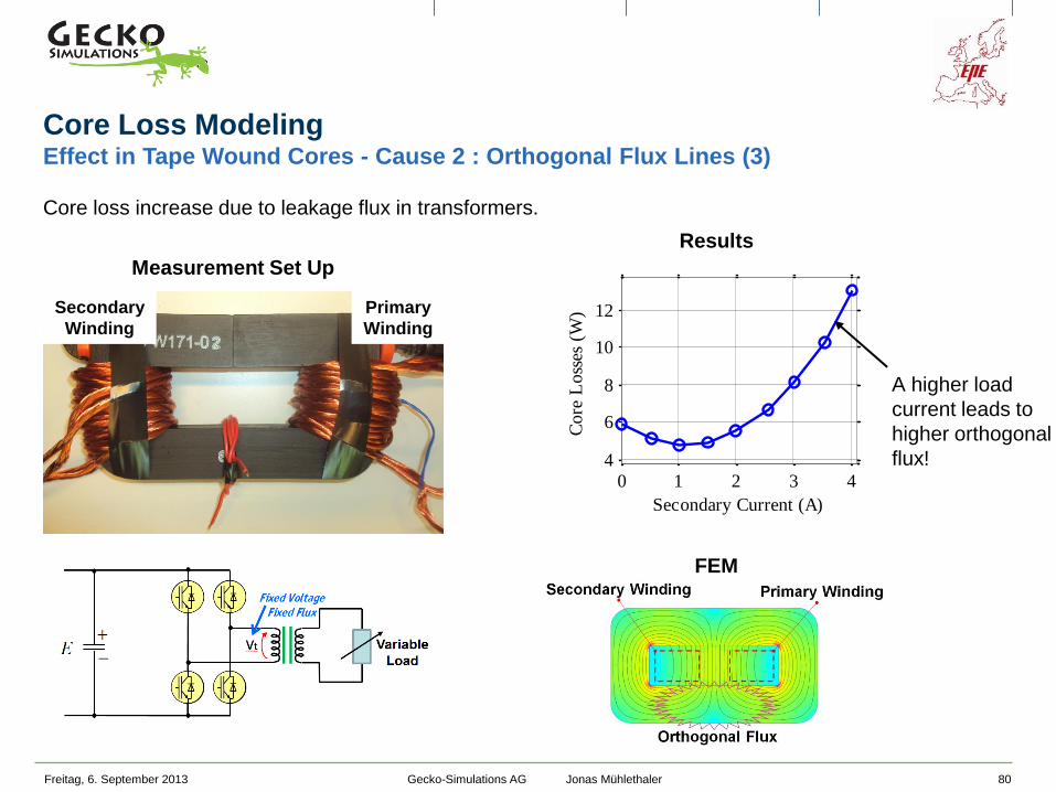
Freitag, 6. September 2013 80
Measurement Set Up
Core loss increase due to leakage flux in transformers.
Primary
Winding
Secondary
Winding
Results
0 1 2 3 4
4
6
8
10
12
Secondary Current (A)
Core
Loss
es (
W)
Core Loss Modeling Effect in Tape Wound Cores - Cause 2 : Orthogonal Flux Lines (3)
FEM
A higher load
current leads to
higher orthogonal
flux!
Gecko-Simulations AG Jonas Mühlethaler

Freitag, 6. September 2013 81
Figures from [10]
In [10] a core loss increase with increasing air gap length has been observed.
Core Loss Modeling Effect in Tape Wound Cores - Cause 2 : Orthogonal Flux Lines (4)
[10] H. Fukunaga, T. Eguchi, K. Koga, Y. Ohta, and H. Kakehashi, “High Performance Cut Cores Prepared From
Crystallized Fe-Based Amorphous Ribbon”, in IEEE Transactions on Magnetics, vol. 26, no. 5, 1990.
Gecko-Simulations AG Jonas Mühlethaler

Freitag, 6. September 2013 82
Example Core Loss Modeling
Photo & Dimensions
Material
Grain-oriented steel (M165-35S)
An approximately homogeneous
flux density distribution inside the core.
Reluctance Model
Flux Density Distribution
Flux Density Waveform
Gecko-Simulations AG Jonas Mühlethaler
MATLAB Presentation

Outline
Freitag, 6. September 2013 83
Magnetic Circuit Modeling
Core Loss Modeling
Winding Loss Modeling
Thermal Modeling
Multi-Objective Optimization
Summary & Conclusion
Gecko-Simulations AG Jonas Mühlethaler

Freitag, 6. September 2013 84
Faraday’s Law
Winding Loss Modeling Skin Effect (1)
H-field in conductor
Induced Eddy Currents
Ampere’s Law
Gecko-Simulations AG Jonas Mühlethaler
𝐻d𝑙 = 𝐽d𝐴
𝐸d𝑙 = −d
d𝑡 𝐵d𝐴
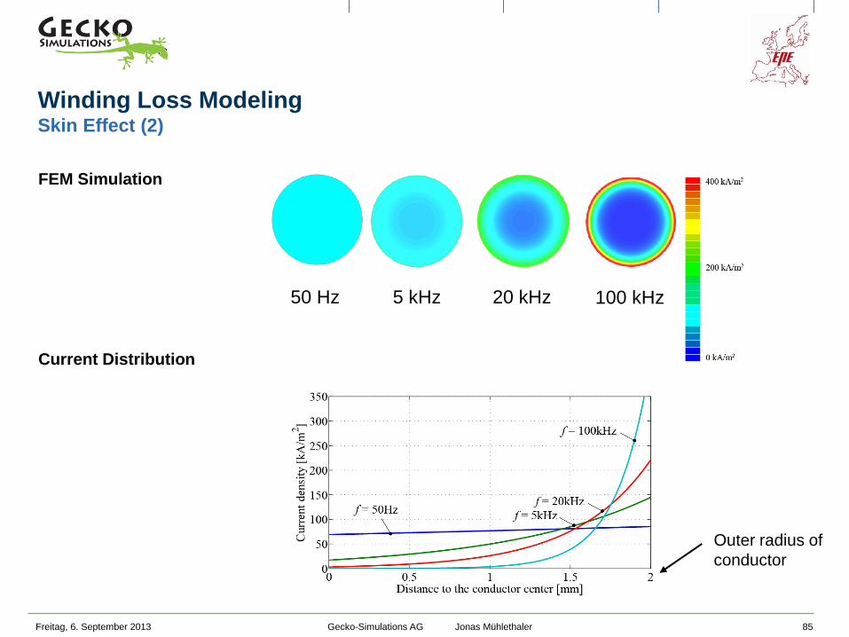
Freitag, 6. September 2013 85
Winding Loss Modeling Skin Effect (2)
FEM Simulation
Current Distribution
50 Hz 5 kHz 20 kHz 100 kHz
Outer radius of
conductor
Gecko-Simulations AG Jonas Mühlethaler

Winding Loss Modeling Skin Effect (3)
Freitag, 6. September 2013 86
Skin Depth
0
1
f
Power Loss Increase with Frequency
[19]
2
S R DCˆ( )P F f R I R ( )F f
2
d
(, where the current density has 1/e of surface value)
Gecko-Simulations AG Jonas Mühlethaler

Winding Loss Modeling Skin Effect (4)
Freitag, 6. September 2013 87
Current Distributions
Parallel-connected (not
twisted) conductors!
Figure from [19]
Gecko-Simulations AG Jonas Mühlethaler

Freitag, 6. September 2013 88
Faraday’s Law
Winding Loss Modeling Proximity Effect (1)
H-field of neighboring conductor induces eddy currents
Ampere’s Law
Gecko-Simulations AG Jonas Mühlethaler
𝐻d𝑙 = 𝐽d𝐴
𝐸d𝑙 = −d
d𝑡 𝐵d𝐴

Freitag, 6. September 2013 89
Winding Loss Modeling Proximity Effect (2)
Eddy Currents in
Conductor
Induced Eddy
Currents
Current
Concentration
50 Hz 5 kHz 15 kHz 100 kHz
(He,rms = 35 A/m
parallel to
conductor)
Figures from [19] I I I I
Gecko-Simulations AG Jonas Mühlethaler
Freitag, 6. September 2013 90
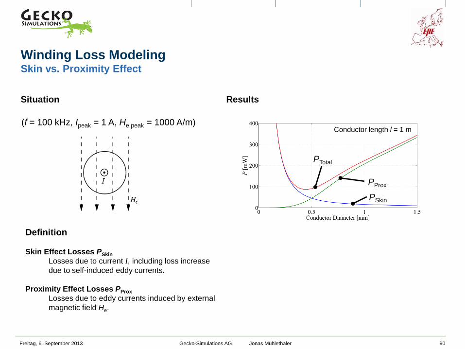
Winding Loss Modeling Skin vs. Proximity Effect
(f = 100 kHz, Ipeak = 1 A, He,peak = 1000 A/m)
Situation
Results
Definition
Skin Effect Losses PSkin
Losses due to current I, including loss increase
due to self-induced eddy currents.
Proximity Effect Losses PProx
Losses due to eddy currents induced by external
magnetic field He.
PSkin
PProx
PTotal
Conductor length l = 1 m
Gecko-Simulations AG Jonas Mühlethaler

Freitag, 6. September 2013 91
Winding Loss Modeling Litz Wire (1) - What are Litz wires?
ww
w.w
ikip
edia
.org
Idea
Implementation
Advantages of Litz wires
HF losses can be reduced
substantially
Disadvantages of Litz wires
High price
Heat dissipation difficult
Higher RDC
Gecko-Simulations AG Jonas Mühlethaler

Freitag, 6. September 2013 92
Winding Loss Modeling Litz Wire (2) - Why Litz Wires Have to be Twisted? (1)
Bundle-Level Skin Effect
Current Distributions
(Faraday’s Law)
(Ampere’s Law)
Internal Proximity
Effect (will be explained later)
Gecko-Simulations AG Jonas Mühlethaler
𝐻d𝑙 = 𝐽d𝐴
𝐸d𝑙 = −d
d𝑡 𝐵d𝐴
Figures from [19]
Freitag, 6. September 2013 93
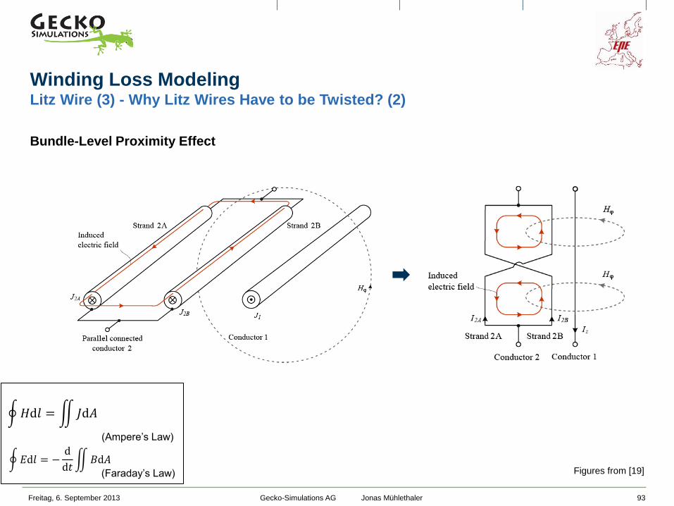
Winding Loss Modeling Litz Wire (3) - Why Litz Wires Have to be Twisted? (2)
Bundle-Level Proximity Effect
Gecko-Simulations AG Jonas Mühlethaler
(Faraday’s Law)
(Ampere’s Law)
𝐻d𝑙 = 𝐽d𝐴
𝐸d𝑙 = −d
d𝑡 𝐵d𝐴
Freitag, 6. September 2013 94
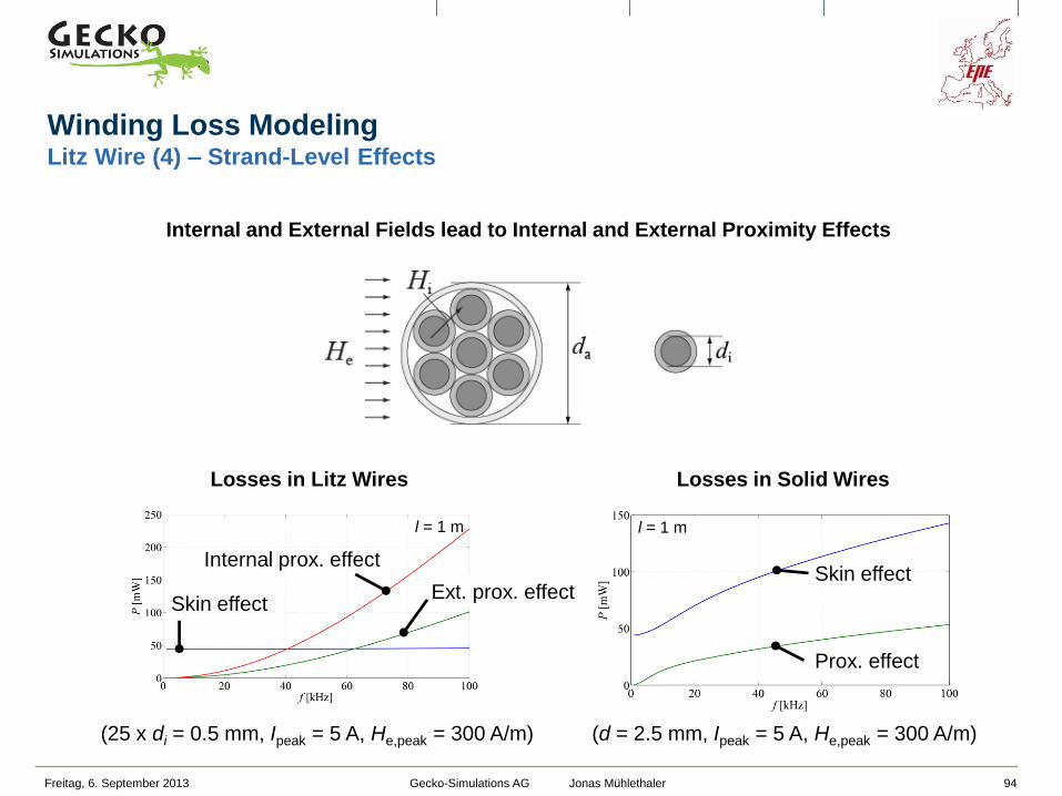
Winding Loss Modeling Litz Wire (4) – Strand-Level Effects
Losses in Litz Wires
Losses in Solid Wires
Internal and External Fields lead to Internal and External Proximity Effects
(25 x di = 0.5 mm, Ipeak = 5 A, He,peak = 300 A/m) (d = 2.5 mm, Ipeak = 5 A, He,peak = 300 A/m)
Skin effect
Internal prox. effect
Ext. prox. effect
l = 1 m
Skin effect
Prox. effect
l = 1 m
Gecko-Simulations AG Jonas Mühlethaler

Freitag, 6. September 2013 95
Winding Loss Modeling Litz Wire (5) – Types of Eddy-Current Effects in Litz Wire
Figure from [11] Ch. R. Sullivan, “Optimal Choice for Number of Strands in a Litz-Wire Transformer
Winding”, in IEEE Transactions on Power Electronics, vol. 14, no. 2, 1999.
Gecko-Simulations AG Jonas Mühlethaler

Freitag, 6. September 2013 96
Winding Loss Modeling Litz Wire (6) – Real Litz Wire
How do “real” Litz wires behave? [12]
[12] H. Rossmanith, M. Doebroenti, M. Albach, and D. Exner, “Measurement and Characterization of High Frequency Losses in Nonideal
Litz Wires”, IEEE Transactions on Power Electronics, vol. 26, no. 11, November 2011
Ideal Litz Wire
(ideally twisted
strands)
Worst Case Litz Wire
(parallel connected
strands, no twisting)
skin,λ skin skin,ideal skin skin,parallel(1 )R R R Skin Effect / Internal Proximity Effect
External Proximity Effect
prox,λ prox prox,ideal prox prox,parallel(1 )R R R
Litz Wire Type 1: 7 bundles with 35 strands each: skin 0.5 / prox 0.99
Litz Wire Type 2: 4 bundles with 61/62 strands each: skin 0.9 / prox 0.99
Operating Point
f = 20 kHz / n = 130 /
di = 0.4 mm
Gecko-Simulations AG Jonas Mühlethaler
Freitag, 6. September 2013 97
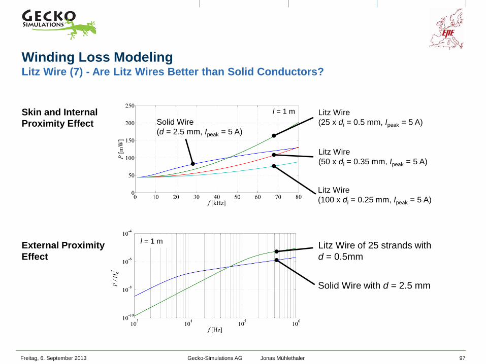
Winding Loss Modeling Litz Wire (7) - Are Litz Wires Better than Solid Conductors?
Skin and Internal
Proximity Effect
External Proximity
Effect
Litz Wire of 25 strands with
d = 0.5mm
Solid Wire with d = 2.5 mm
Litz Wire
(25 x di = 0.5 mm, Ipeak = 5 A) Solid Wire
(d = 2.5 mm, Ipeak = 5 A)
Litz Wire
(100 x di = 0.25 mm, Ipeak = 5 A)
Litz Wire
(50 x di = 0.35 mm, Ipeak = 5 A)
l = 1 m
l = 1 m
Gecko-Simulations AG Jonas Mühlethaler

Freitag, 6. September 2013 98
Winding Loss Modeling Foil Windings Enclosed by Magnetic Material
10 mm x 0.3 mm
Ipeak = 1 A
d = 1.95 mm
Ipeak = 1 A
Advantages of foil windings
HF losses can be reduced
Lower price compared to Litz wire
High filling factor
Disadvantages of foil windings
Increased winding capacitance
Risk of orthogonal flux
Conductor length l = 1 m
Same cross
section!
“Skin” of foil conductor larger
than of round conductor with
same cross section; hence,
skin effect losses lower in foil
conductor.
Gecko-Simulations AG Jonas Mühlethaler
Freitag, 6. September 2013 99
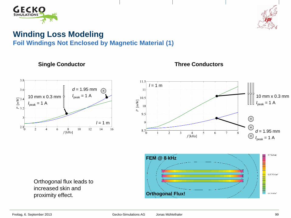
Winding Loss Modeling Foil Windings Not Enclosed by Magnetic Material (1)
FEM @ 8 kHz
Orthogonal Flux!
d = 1.95 mm
Ipeak = 1 A
10 mm x 0.3 mm
Ipeak = 1 A
Three Conductors Single Conductor
10 mm x 0.3 mm
Ipeak = 1 A
d = 1.95 mm
Ipeak = 1 A
l = 1 m
l = 1 m
Orthogonal flux leads to
increased skin and
proximity effect.
Gecko-Simulations AG Jonas Mühlethaler

Freitag, 6. September 2013 100
Winding Loss Modeling Foil Windings Not Enclosed by Magnetic Material (2)
FEM @ 8 kHz
10 mm x 0.3 mm
Ipeak = 1 A
d = 1.95 mm
Ipeak = 1 A
(Foil) Windings with Return Conductors
l = 1 m
Gecko-Simulations AG Jonas Mühlethaler
Freitag, 6. September 2013 101
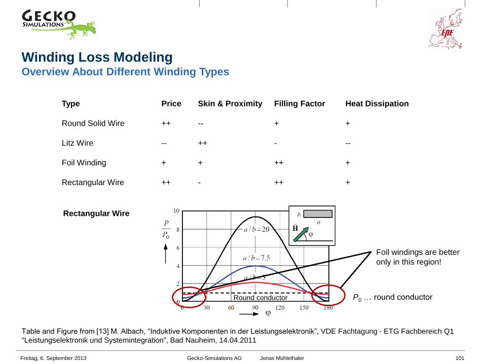
Winding Loss Modeling Overview About Different Winding Types
Type Price Skin & Proximity Filling Factor Heat Dissipation
Round Solid Wire ++ -- + +
Litz Wire -- ++ - --
Foil Winding + + ++ +
Rectangular Wire ++ - ++ +
Table and Figure from [13] M. Albach, “Induktive Komponenten in der Leistungselektronik”, VDE Fachtagung - ETG Fachbereich Q1
"Leistungselektronik und Systemintegration", Bad Nauheim, 14.04.2011
Rectangular Wire
P0 … round conductor Round conductor
Foil windings are better
only in this region!
Gecko-Simulations AG Jonas Mühlethaler

Freitag, 6. September 2013 102
2
S F DCˆ( )P F f R I
with
F
DC
0
sinh sin
4 cosh cos
1
1
v v vF
v v
Rbh
hv
f
Winding Loss Modeling Skin Effect of Foil Conductor
(Loss per unit length)
FF evaluated
Geometry Considered
Current Distribution
[19]
Gecko-Simulations AG Jonas Mühlethaler

Freitag, 6. September 2013 103
2
P F DC Sˆ( )P G f R H
with
2
F
DC
0
sinh sin
cosh cos
1
1
v vG b v
v v
Rbh
hv
f
Winding Loss Modeling Proximity Effect of Foil Conductor
(Loss per unit length)
GF evaluated
Geometry Considered
Current Distribution
(b = 1 m)
[19]
Gecko-Simulations AG Jonas Mühlethaler
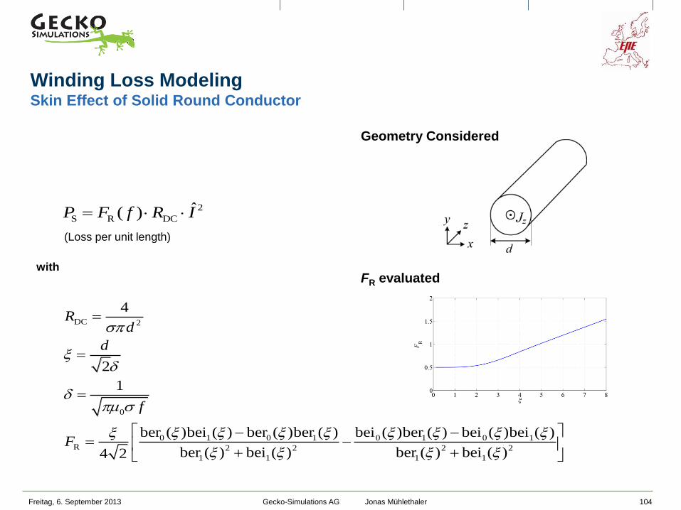
Freitag, 6. September 2013 104
2
S R DCˆ( )P F f R I
with
DC 2
0
0 1 0 1 0 1 0 1R 2 2 2 2
1 1 1 1
4
2
1
ber ( )bei ( ) ber ( )ber ( ) bei ( )ber ( ) bei ( )bei ( )
ber ( ) bei ( ) ber ( ) bei ( )4 2
Rd
d
f
F
(Loss per unit length)
Winding Loss Modeling Skin Effect of Solid Round Conductor
FR evaluated
Geometry Considered
Gecko-Simulations AG Jonas Mühlethaler

Freitag, 6. September 2013 105
2
P R DC Sˆ( )P G f R H
with
DC 2
0
2 2
2 1 2 1 2 1 2 1R 2 2 2 2
0 0 0 0
4
2
1
ber ( )ber ( ) ber ( )bei ( ) bei ( )bei ( ) bei ( )ber ( )
ber ( ) bei ( ) ber ( ) bei ( )2 2
Rd
d
f
dG
(Loss per unit length)
Winding Loss Modeling Proximity Effect of Solid Round Conductor
GR evaluated
Geometry Considered
(d = 1 m)
Gecko-Simulations AG Jonas Mühlethaler

Freitag, 6. September 2013 106
Winding Loss Modeling Skin and Proximity Effect of Litz Wire
(Loss per unit length)
2
S DC R
ˆ( )
IP n R F f
n
Skin Effect
(Loss per unit length)
P,e ,iP PP P P
Proximity Effect
2
DC R e 2
a
2
2ˆ
( )2
In R G f H
d
Losses in Litz Wires
(25 x di = 0.5 mm, Ipeak = 5 A, He,peak = 300 A/m)
Skin effect
Internal prox. effect
Ext. prox. effect
l = 1 m
Average internal field Hi
under the assumption of a
homogeneous current
distribution inside the Litz
wire.
Gecko-Simulations AG Jonas Mühlethaler
Freitag, 6. September 2013 107
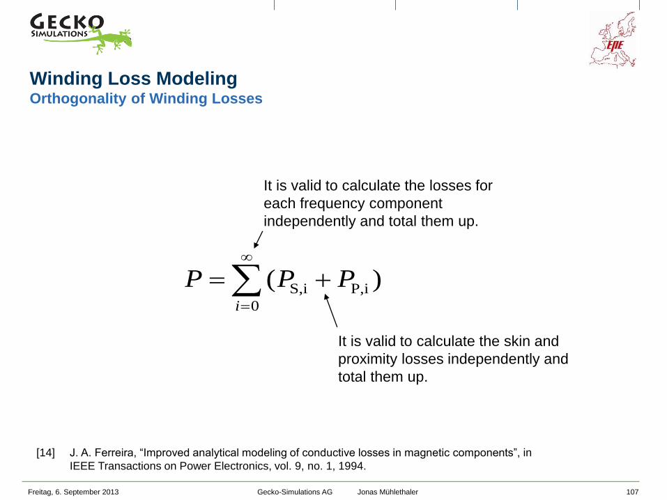
Winding Loss Modeling Orthogonality of Winding Losses
S,i P,i
0
( )i
P P P
It is valid to calculate the skin and
proximity losses independently and
total them up.
It is valid to calculate the losses for
each frequency component
independently and total them up.
[14] J. A. Ferreira, “Improved analytical modeling of conductive losses in magnetic components”, in
IEEE Transactions on Power Electronics, vol. 9, no. 1, 1994.
Gecko-Simulations AG Jonas Mühlethaler

Winding Loss Modeling Calculation of External Field He (1D - Approach)
Freitag, 6. September 2013 108
with
avg left right
1
2H H H
Un-Gapped Transformer Cores
2 2
DC R/F R/F avg,m m
1
ˆ ˆM
m
P R F I NM NG H l
2
DC R/F R/
23
2
F
F m
4ˆ12
1MP R I F NM GMN l
b
it is
where
N … the number of conductors per layer
(i.e. N = 1 for foil windings)
M … the number of layers.
Figure from [19]
leftH avgH rightH
Gecko-Simulations AG Jonas Mühlethaler
(Ampere’s Law)
𝐻d𝑙 = 𝐽d𝐴

Winding Loss Modeling Short Foil Conductors
Freitag, 6. September 2013 109
“Porosity Factor”
L
F
Nb
b
'
Redefinition of Parameters
''
h
0
1'
'f
Gecko-Simulations AG Jonas Mühlethaler

Winding Loss Modeling FEM Simulations : Foil Windings
Freitag, 6. September 2013 110
N = 2 x 10
h = 0.3 mm
bL = 33 mm
bF = 37 mm
Ipeak = 1 A
N = 2 x 7
h = 0.4 mm
bL = 37 mm
bF = 37 mm
Ipeak = 1 A
Error < 6.5%
Gecko-Simulations AG Jonas Mühlethaler

Winding Loss Modeling Calculation of External Field He (2D - Approach)
Freitag, 6. September 2013 111
Gapped cores: 2D approach is necessary !
Gecko-Simulations AG Jonas Mühlethaler

Winding Loss Modeling Effect of the Air Gap Fringing Field
Freitag, 6. September 2013 112
The air gap is replaced by a fictitious
current, which …
… has the value equal to the magneto-motive
force (mmf) across the air gap.
2
1
m,air aird
P
P
V R H l
P1
P2
P1
P2
2
1
m,air d
P
P
V I H l
I
An accurate air gap reluctance model is needed!
Gecko-Simulations AG Jonas Mühlethaler

Winding Loss Modeling Effect of the Core Material
Freitag, 6. September 2013 113
“Pushing the walls away”
The method of images (mirroring)
Gecko-Simulations AG Jonas Mühlethaler
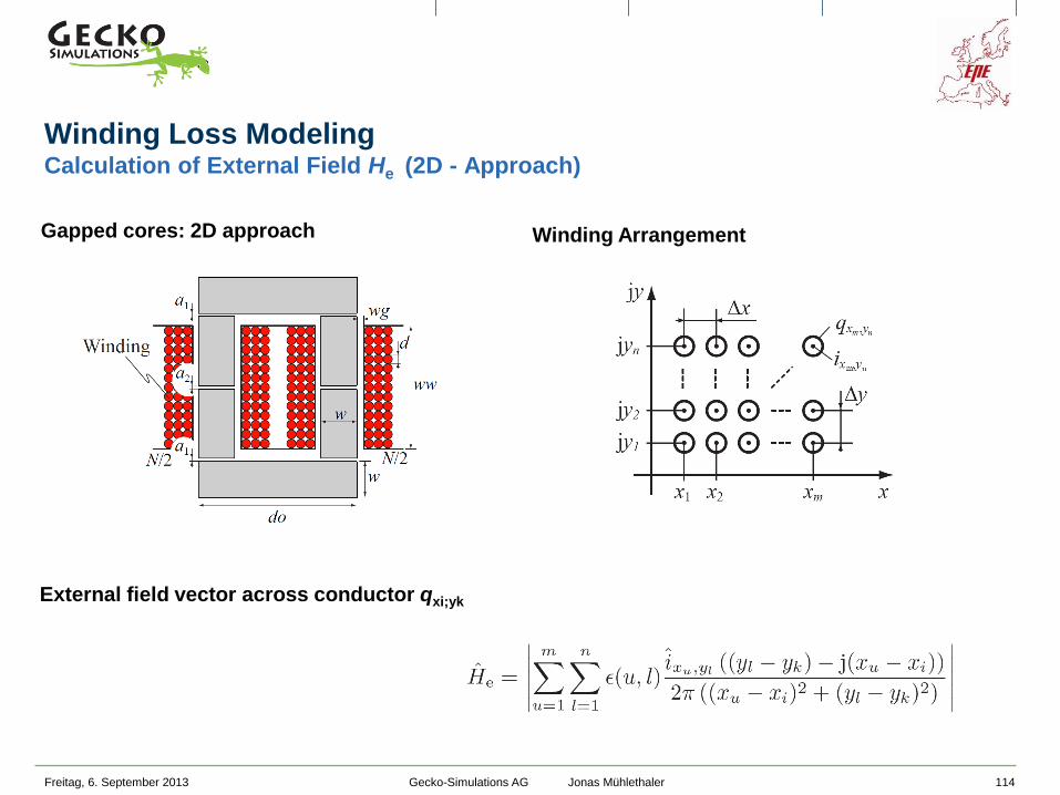
Winding Loss Modeling Calculation of External Field He (2D - Approach)
Freitag, 6. September 2013 114
Gapped cores: 2D approach
Winding Arrangement
External field vector across conductor qxi;yk
Gecko-Simulations AG Jonas Mühlethaler
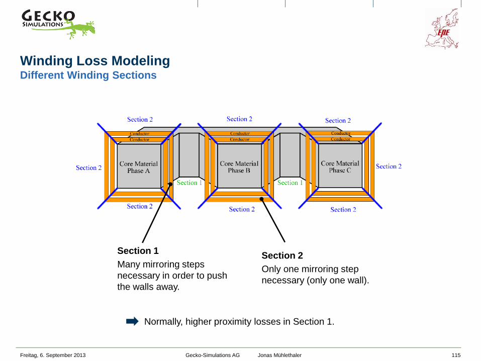
Winding Loss Modeling Different Winding Sections
Freitag, 6. September 2013 115
Section 2
Only one mirroring step
necessary (only one wall).
Section 1
Many mirroring steps
necessary in order to push
the walls away.
Normally, higher proximity losses in Section 1.
Gecko-Simulations AG Jonas Mühlethaler

Major Simplification
- magnetic field of the induced eddy
currents neglected.
- This can be problematic at frequencies
above (rule-of-thumb) [15]
Freitag, 6. September 2013 116
max 2
0
2.56f
d
Results of considered winding arrangements
f-range f < fmax f > fmax
Error < 5% > 5% (always < 25%)
Winding Loss Modeling FEM Simulations : Round Windings (Including Litz Wire Windings) (1)
[15] A. Van den Bossche, V. C. Valchev, “Inductors and Transformers for
Power Electronics”, CRC Press. Taylor & Francis Group, 2005
Gecko-Simulations AG Jonas Mühlethaler

Freitag, 6. September 2013 117
Winding Loss Modeling FEM Simulations : Round Windings (Including Litz Wire Windings) (2)
FEM Simulation
maxf
maxf
maxf
Results
Gecko-Simulations AG Jonas Mühlethaler

Winding Loss Modeling Methods to Decrease Winding Losses (1)
Freitag, 6. September 2013 118
Interleaving
Litz Wire
Optimal Solid Wire Thickness
(f = 100 kHz, Ipeak = 1 A, He,peak = 1000 A/m)
(f = 20 kHz, Ipeak = 1 A, b = 20 cm, He,peak = 1000 A/m)
Push this point to
higher frequencies!
Optimal Foil Thickness
Increase number
of strands.
(resp.: find optimal
number of strands)
[19]
PSkin
PProx PTotal
l = 1 m
l = 1 m
PSkin
PProx
PTotal
l = 1 m
Avoid Orthogonal Flux in Foil Windings
Gecko-Simulations AG Jonas Mühlethaler

Winding Loss Modeling Methods to Decrease Winding Losses (2)
Freitag, 6. September 2013 119
Arrangement of Windings
Proximity losses increase in
more compact winding
arrangements.
Gecko-Simulations AG Jonas Mühlethaler

Winding Loss Modeling Methods to Decrease Winding Losses (3)
Freitag, 6. September 2013 120
Aluminum vs. Copper [13]
Aluminum (vs. Copper):
- Lighter
- Lower costs
- Lower Conductivity = 38 · 106 1/(m)
( Copper: = 58 · 106 1/(m) )
Lower Skin Depth!
Skin- and DC losses higher than in copper
conductors.
d = 0.25 mm
d = 0.50 mm
d = 0.75 mm
d = 1.00 mm
Proximity losses are lower in aluminum
conductors over a wide frequency range.
Figure shows a comparison of single round
solid conductors in external field.
[13] M. Albach, “Induktive Komponenten in der Leistungselektronik”, VDE Fachtagung - ETG Fachbereich Q1
"Leistungselektronik und Systemintegration", Bad Nauheim, 14.04.2011
Gecko-Simulations AG Jonas Mühlethaler

Freitag, 6. September 2013 121
Example Winding Loss Modeling
Photo & Dimensions
Material
Grain-oriented steel (M165-35S)
Current Waveform
Demonstration in MATLAB
Gecko-Simulations AG Jonas Mühlethaler

Outline
Freitag, 6. September 2013 122
Magnetic Circuit Modeling
Core Loss Modeling
Winding Loss Modeling
Thermal Modeling
Multi-Objective Optimization
Summary & Conclusion
Gecko-Simulations AG Jonas Mühlethaler

Freitag, 6. September 2013 123
Thermal Modeling Motivation & Model (1)
Ambient
Temperature
Thermal modeling is important to …
… avoid overheating.
… improve loss calculation (since the losses
depend on temperature).
Motivation
Gecko-Simulations AG Jonas Mühlethaler

Freitag, 6. September 2013 124
Thermal Modeling Motivation & Model (2)
Model
Inductor
Transformer
Determination of thermal resistors is challenging!
Gecko-Simulations AG Jonas Mühlethaler

Freitag, 6. September 2013 125
Conduction
Independent of temperature T for most materials
Difficult to determine interfaces between materials
Rth T
P f (T)
Rth T
Pl
A
Rth T
P1
A
P eff A1(Tb4 Ta
4)
Thermal Modeling Heat Transfer Mechanisms
Convection
Combined effect of conduction and fluid flow
Changes with changing absolute temperature (nonlinear)
Good empirical calculation approach available
Radiation
Small compared to other mechanisms
Modeling the system is demanding
(nonlinear eq. / to describe which components “sees”
the other component).
Gecko-Simulations AG Jonas Mühlethaler

Freitag, 6. September 2013 126
th
1TR
P A
is a coefficient that is influenced by …
… the absolute temperature,
… the fluid property,
… the flow rate of the fluid,
… the dimensions of the considered surface,
… orientation of the considered surface,
… and the surface texture.
Thermal Modeling Thermal Resistance Calculation : (Natural) Convection (1)
Gecko-Simulations AG Jonas Mühlethaler

Freitag, 6. September 2013 127
Empirical solutions known for …
vertical plane horizontal plane -top:
- bottom :
gap - horizontal:
- vertical:
and more …
Thermal Modeling Thermal Resistance Calculation : (Natural) Convection (2)
Gecko-Simulations AG Jonas Mühlethaler

Freitag, 6. September 2013 128
Structure of Empirical Solutions - Theory
Name Measure of …
Nusselt number
Nu
… improvement of heat transfer compared to the case with
hypothetical static fluid.
Grashof number
Gr
… ration between buoyancy and frictional force of fluid.
Prandtl number
Pr
… ratio between viscosity and heat conductivity of fluid.
Rayleigh number
Ra
… flow condition (laminar or turbulent) of fluid.
),(1
PrGrfl
AA
lNu
Tv
glGr
3
3
air)(for7.0Pr
GrPrRa
l
PrGrNu
),(
Procedure
AR
1th ),( PrGrNu
Thermal Modeling Thermal Resistance Calculation : (Natural) Convection (3)
g gravity of earth: 9.81 m/s2
l characteristic length
volumetric thermal expansion coefficient : 1/T (air)
v kinematic viscosity: 162.6 ·10-7 m2/s (air)
is the heat conductivity of the fluid
air = 25.873 mW/(m K) @ 20C [16]
[16] VDI Heat Atlas, Springer-Verlag, Berlin, 2010
Gecko-Simulations AG Jonas Mühlethaler

Freitag, 6. September 2013 129
Structure of Empirical Solutions - Example
l
PrGrNu
),(
Vertical Plane
AP
TR
1th
26/1
1387.0825.0 PrfRaNu
9/1616/9
1
492.01
Prf
Thermal Modeling Thermal Resistance Calculation : (Natural) Convection (4)
Increase of Winding Surface
Reference:
[16] VDI Heat Atlas, Springer-Verlag, Berlin, 2010
(l = h)
Example
(h = 10 cm, Tp = 60 C, Ta = 20 C, A = h · h)
Rth = 16.6 K/W
Tp Ta
Gecko-Simulations AG Jonas Mühlethaler

Freitag, 6. September 2013 130
Thermal Modeling Thermal Resistance Calculation : Conduction
Overview
Round Conductor Foil Conductor
Normally, with natural
convection it is
Rth,W << Rth,WA
Rth,W is difficult to
determine. One difficulty
is, e.g., to model the
influence of pressure on
the thermal resistance.
Litz wire shows low
thermal conductivity.
Gecko-Simulations AG Jonas Mühlethaler

Freitag, 6. September 2013 131
Example Thermal Modeling (1)
l
PrGrNu
),(
AP
TR
1th
1/5 4
2 2
1/3 4
2 2
0.766 ( ( )) for ( ) 7 10
0.15 ( ( )) for ( ) 7 10
Ra f Pr Ra f PrNu
Ra f Pr Ra f Pr
20/1111/20
2
0.3221f
Pr
Tv
glGr
3
3
GrPrRa
air)(for7.0Pr
(1) Horizontal Plane - Top
g gravity of earth: 9.81 m/s2
l characteristic length : l = a*b / ( 2 ( a+b ) )
volumetric thermal expansion coefficient : 1/T (air)
v kinematic viscosity: 162.6 ·10-7 m2/s (air)
with
Resistor Rth is now
calculated for one
operating point!
( more iterations
are necessary!)
(laminar)
(turbulent)
Gecko-Simulations AG Jonas Mühlethaler

Freitag, 6. September 2013 132
Example Thermal Modeling (2)
(2) Core to Winding
CF
K1.05
W
lR
A
W WAR R
Heat flow via
mechanical
attachment has not
been considered.
Quantity Values
Rth,CA 17.4 K/W
Rth,WA 5.8 K/W
Drawing represents the
cross-section of one
coil former side (there
are total 2 x 4 coil
former sides).
Gecko-Simulations AG Jonas Mühlethaler

Outline
Freitag, 6. September 2013 133
Magnetic Circuit Modeling
Core Loss Modeling
Winding Loss Modeling
Thermal Modeling
Multi-Objective Optimization
Summary & Conclusion
Gecko-Simulations AG Jonas Mühlethaler

Freitag, 6. September 2013 134
Photo of Converter Converter Specifications
Simplified Schematic
Multi-Objective Optimization – Volume vs. Losses Introduction to the PFC Rectifier
Gecko-Simulations AG Jonas Mühlethaler
Goal: Design boost inductor such that the max. current ripple is 4A.

Freitag, 6. September 2013 135
Selected Inductor Shape
Material
Grain-oriented steel
(M165-35S,
lam. thickness 0.35 mm)
Photo of Inductor
Multi-Objective Optimization – Volume vs. Losses Boost Inductor
Gecko-Simulations AG Jonas Mühlethaler
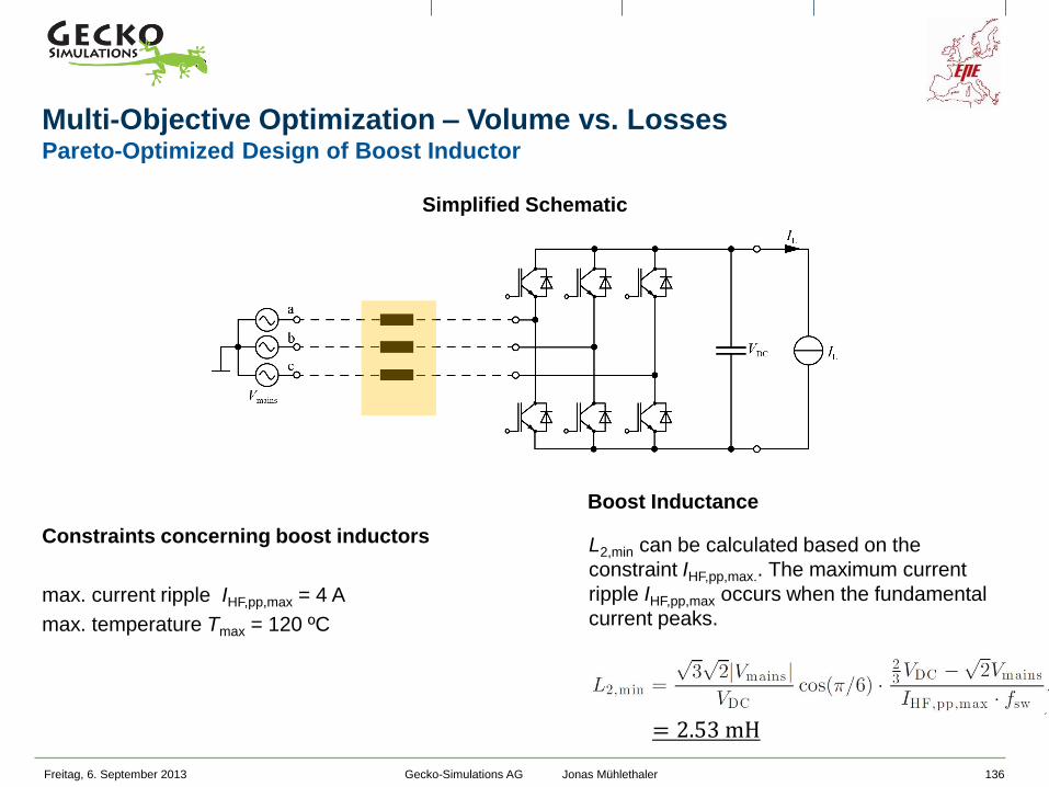
Freitag, 6. September 2013 136
Constraints concerning boost inductors
max. current ripple IHF,pp,max = 4 A
max. temperature Tmax = 120 ºC
Simplified Schematic
Multi-Objective Optimization – Volume vs. Losses Pareto-Optimized Design of Boost Inductor
Gecko-Simulations AG Jonas Mühlethaler
L2,min can be calculated based on the
constraint IHF,pp,max.. The maximum current
ripple IHF,pp,max occurs when the fundamental
current peaks.
Boost Inductance
= 2.53 mH
Freitag, 6. September 2013 137
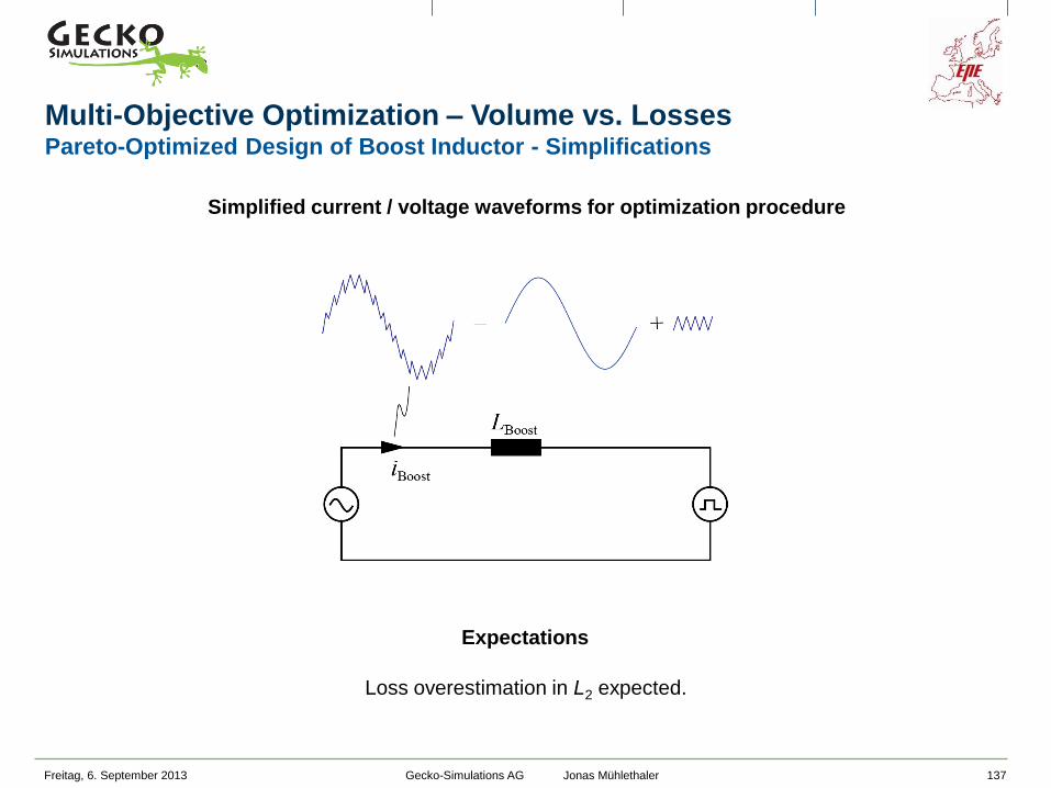
Multi-Objective Optimization – Volume vs. Losses Pareto-Optimized Design of Boost Inductor - Simplifications
Loss overestimation in L2 expected.
Simplified current / voltage waveforms for optimization procedure
Expectations
Gecko-Simulations AG Jonas Mühlethaler

Freitag, 6. September 2013 138
Multi-Objective Optimization – Volume vs. Losses Pareto-Optimized Design of Boost Inductor - Design Space in GeckoMAGNETICS
Gecko-Simulations AG Jonas Mühlethaler
LBoost = 2.53 mH
Tmax = 120 ºC
Solid round wire with fill factor 0.3
Split windings
UI 39 – UI 90 cores of DIN41302
Material M165-35S
gap 2.0 … 3.0 mm (by 0.25 mm)
70 – 90 stacked sheets (by 10)
Start
Core
Winding

Freitag, 6. September 2013 139
Multi-Objective Optimization – Volume vs. Losses Pareto-Optimized Design of Boost Inductor - Waveform/Cooling in GeckoMAGNETICS
Gecko-Simulations AG Jonas Mühlethaler
ILF,peak = 21.8 A
Voltage Time Area = 𝛿100 ∙
23𝑉DC − 2𝑉mains
𝐼HF,pp,max ∙ 𝑓sw=
3 2 𝑉mains𝑉𝐷𝐶
cos𝜋
6∙
23𝑉DC − 2𝑉mains
𝐼HF,pp,max ∙ 𝑓sw= 0.01 Vs
Forced convection
(-> 3 m/s)
Waveform
Cooling

Freitag, 6. September 2013 140
1) A reluctance model is introduced to describe the electric /
magnetic interface, i.e. L = f(i).
2) Core losses are calculated.
3) Winding losses are calculated.
4) Inductor temperature is calculated.
Multi-Objective Optimization – Volume vs. Losses Pareto-Optimized Design of Boost Inductor - Performing Calculation
Procedure
Air gap stray field
Non-linearity of core material
Considered effects
DC Bias
Different flux waveforms
Wide range of flux densities
and frequencies
Skin and proximity effect
Stray field proximity effect
Effect of core to magnetic
field distribution
Gecko-Simulations AG Jonas Mühlethaler

Freitag, 6. September 2013 141
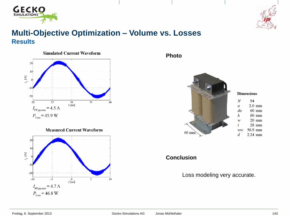
Multi-Objective Optimization – Volume vs. Losses Pareto-Optimized Design of Boost Inductor - Results
Gecko-Simulations AG Jonas Mühlethaler
Filter Losses vs. Filter Volume
Pareto Front
Prototype built
Pareto-front

Freitag, 6. September 2013 142
Multi-Objective Optimization – Volume vs. Losses Detailed Modeling in GeckoMAGNETICS
Gecko-Simulations AG Jonas Mühlethaler
GeckoCIRCUITS GeckoMAGNETICS
Freitag, 6. September 2013 143
Photo
Loss modeling very accurate.
Conclusion
Multi-Objective Optimization – Volume vs. Losses Results
Gecko-Simulations AG Jonas Mühlethaler

Outline
Freitag, 6. September 2013 144 Gecko-Simulations AG Jonas Mühlethaler
Magnetic Circuit Modeling
Core Loss Modeling
Winding Loss Modeling
Thermal Modeling
Multi-Objective Optimization
Summary & Conclusion
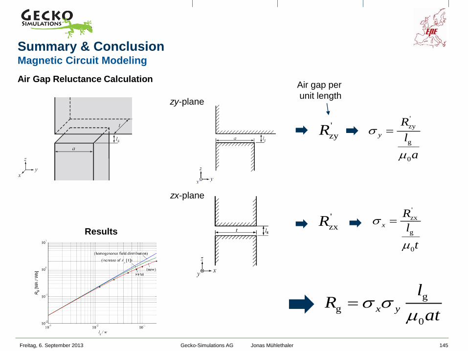
Freitag, 6. September 2013 145 Gecko-Simulations AG Jonas Mühlethaler
zy-plane
zx-plane
'
zyR
Summary & Conclusion Magnetic Circuit Modeling
g
g
0
x y
lR
at
Results
Air Gap Reluctance Calculation Air gap per
unit length
'
zxR
'
zy
g
0
y
R
l
a
'
zx
g
0
x
R
l
t
Freitag, 6. September 2013 146 Gecko-Simulations AG Jonas Mühlethaler
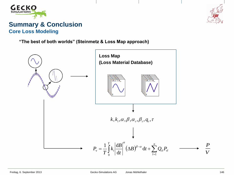
Loss Map
(Loss Material Database)
n
l
ll
T
i PQtBt
Bk
TP
1
rr
0
v dd
d1
r r r, , , , , , ,ik k q
P
V
“The best of both worlds” (Steinmetz & Loss Map approach)
Summary & Conclusion Core Loss Modeling

Freitag, 6. September 2013 147 Gecko-Simulations AG Jonas Mühlethaler
Gapped cores: 2D approach
Summary & Conclusion Winding Loss Modeling
Losses in Litz Wires
Skin effect
Internal prox. effect
Ext. prox. effect
Optimal Solid Wire Thickness
PSkin
PProx
PTotal
(f = 100 kHz, Ipeak = 1 A, He,peak = 1000 A/m)
10 mm x 0.3 mm
Ipeak = 1 A
d = 1.95 mm
Ipeak = 1 A
Foil vs. Round Conductors
l = 1 m l = 1 m
l = 1 m

Freitag, 6. September 2013 148 Gecko-Simulations AG Jonas Mühlethaler
Automated Measurement System
Core Material Database
GeckoDB
Magnetics Design Software
GeckoMAGNETICS
Verification
(e.g. with Calorimeter)
Circuit Simulator
GeckoCIRCUITS
Summary & Conclusion Magnetic Design Environment
Prototype

Freitag, 6. September 2013 149 Gecko-Simulations AG Jonas Mühlethaler
PFC Rectifier
Summary & Conclusion Multi-Objective Optimization
Inductor Pareto Front

150

Additional References
Freitag, 6. September 2013 152 Gecko-Simulations AG Jonas Mühlethaler
[6] J. Mühlethaler, J.W. Kolar, and A. Ecklebe, “A Novel Approach for 3D Air Gap Reluctance Calculations”,
in Proc. of the ICPE - ECCE Asia, Jeju, Korea, 2011
[9] J. Mühlethaler, J. Biela, J.W. Kolar, and A. Ecklebe, “Improved Core Loss Calculation for Magnetic
Components Employed in Power Electronic Systems”, in Proc. of the APEC, Ft. Worth, TX, USA, 2011.
[19] Jürgen Biela, “Wirbelstromverluste in Wicklungen induktiver Bauelemente”, Part of script to lecture Power
Electronic Systems 1, ETH Zurich, 2007
[20] J. Mühlethaler, J.W. Kolar, and A. Ecklebe, “Loss Modeling of Inductive Components Employed in
Power Electronic Systems”, in Proc. of the ICPE - ECCE Asia, Jeju, Korea, 2011
[21] J. Mühlethaler, J. Biela, J.W. Kolar, and A. Ecklebe, “Core Losses under DC Bias Condition based
on Steinmetz Parameters”, in Proc. of the IPEC - ECCE Asia, Sapporo, Japan, 2010.
[22] B. Cougo, A. Tüysüz, J. Mühlethaler, J.W. Kolar, “Increase of Tape Wound Core Losses Due to
Interlamination Short Circuits and Orthogonal Flux Components”, in Proc. of the IECON, Melbourne, 2011.
[23] J. Mühlethaler, M. Schweizer, R. Blattmann, J.W. Kolar, and A. Ecklebe, “Optimal Design of LCL Harmonic
Filters for Three-Phase PFC Rectifiers”, in Proc. of the IECON, Melbourne, 2011
Contact Jonas Mühlethaler
www.gecko-simulations.com


