Standard Deviation

68% of measurements are found within one standard deviation σ from the mean μ; 95% are found within 1.96 times the standard deviation from the mean.

ExampleA population of liver cells has p.H. with a mean of 5.61 and a standard deviation of 0.33. What are the upper and lower limits between which 95% of the cells are found? If a cell has a p.H. of 6.10 is it unusual?Solution1) 95% of cells will be within 5.61 ± (1.96 x 0.33) = 5.61 ± 0.65 = between 4.96 and 6.262) A p.H. of 6.10 is well within these limits so it is not unusual.

The Estimate of the Standard Deviation: We divide by N -1 and not N because we set the mean to be in the middle of the sample. It might not, in fact be there, and so using N tends to underestimate the standard deviation. N -1 is called the degrees of freedom

The mean of a sample is likely to vary (but by less than individuals) because you may have picked by chance samples with more high values of the measurement than average or more low values. The variability of the estimate of the mean is easily calculated and is called the standard error of the mean, SE, which is given by the expression: SE = s /√N

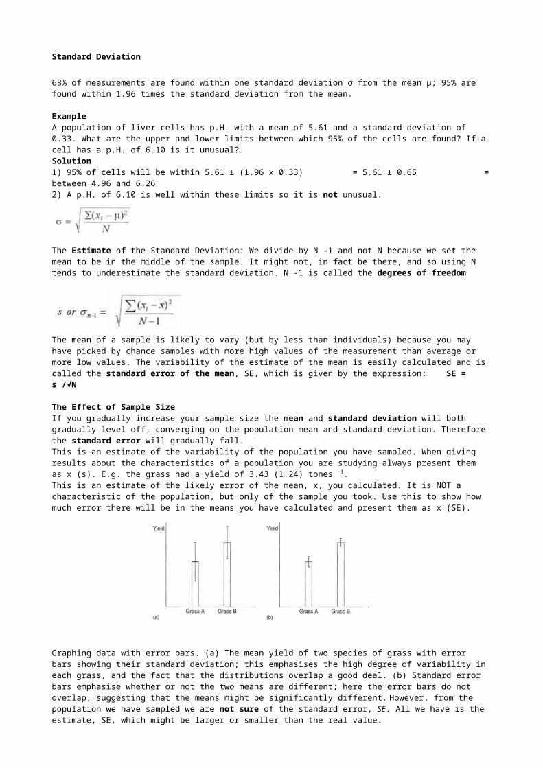
The Effect of Sample SizeIf you gradually increase your sample size the mean and standard deviation will both gradually level off, converging on the population mean and standard deviation. Therefore the standard error will gradually fall.This is an estimate of the variability of the population you have sampled. When giving results about the characteristics of a population you are studying always present them as x (s). E.g. the grass had a yield of 3.43 (1.24) tones -1.This is an estimate of the likely error of the mean, x, you calculated. It is NOT a characteristic of the population, but only of the sample you took. Use this to show how much error there will be in the means you have calculated and present them as x (SE).

Graphing data with error bars. (a) The mean yield of two species of grass with error bars showing their standard deviation; this emphasises the high degree of variability in each grass, and the fact that the distributions overlap a good deal. (b) Standard error bars emphasise whether or not the two means are different; here the error bars do not overlap, suggesting that the means might be significantly different. However, from the population we have sampled we are not sure of the standard error, SE. All we have is the estimate, SE, which might be larger or smaller than the real value.

The t DistributionFor this reason the mean has a broader distribution relative to SE called the t distribution. This is especially wide when the sample size (and hence the number of degrees of freedom, N -1) is low. However, it approaches the normal distribution when the sample size is high and hence when the estimated standard error SE approaches that of the population SE.

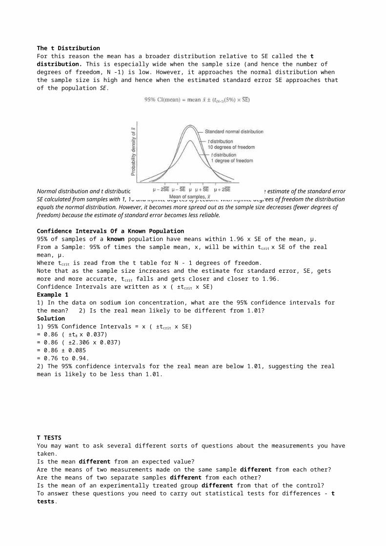
Normal distribution and t distribution. The distribution of sample means x relative to the estimate of the standard error SE calculated from samples with 1, 10 and infinite degrees of freedom. With infinite degrees of freedom the distribution equals the normal distribution. However, it becomes more spread out as the sample size decreases (fewer degrees of freedom) because the estimate of standard error becomes less reliable.

Confidence Intervals Of a Known Population95% of samples of a known population have means within 1.96 x SE of the mean, μ. From a Sample: 95% of times the sample mean, x, will be within tcrit x SE of the real mean, μ.Where tcrit is read from the t table for N - 1 degrees of freedom.Note that as the sample size increases and the estimate for standard error, SE, gets more and more accurate, tcrit falls and gets closer and closer to 1.96.Confidence Intervals are written as x ( ±tcrit x SE)Example 11) In the data on sodium ion concentration, what are the 95% confidence intervals for the mean? 2) Is the real mean likely to be different from 1.01?Solution1) 95% Confidence Intervals = x ( ±tcrit x SE)= 0.86 ( ±t8 x 0.037)= 0.86 ( ±2.306 x 0.037)= 0.86 ± 0.085= 0.76 to 0.94.2) The 95% confidence intervals for the real mean are below 1.01, suggesting the real mean is likely to be less than 1.01.

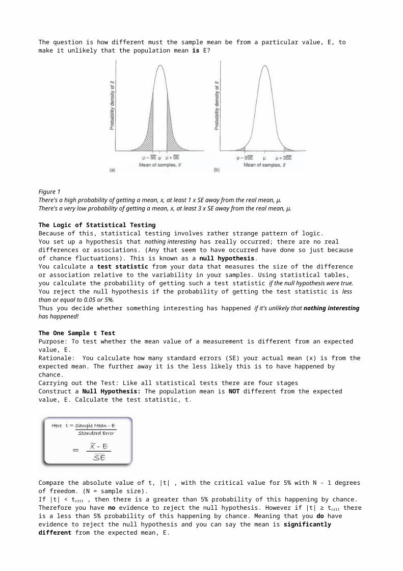
T TESTSYou may want to ask several different sorts of questions about the measurements you have taken.Is the mean different from an expected value? Are the means of two measurements made on the same sample different from each other? Are the means of two separate samples different from each other? Is the mean of an experimentally treated group different from that of the control?To answer these questions you need to carry out statistical tests for differences - t tests.The question is how different must the sample mean be from a particular value, E, to make it unlikely that the population mean is E?

Figure 1There's a high probability of getting a mean, x, at least 1 x SE away from the real mean, μ. There's a very low probability of getting a mean, x, at least 3 x SE away from the real mean, μ.

The Logic of Statistical TestingBecause of this, statistical testing involves rather strange pattern of logic.You set up a hypothesis that nothing interesting has really occurred; there are no real differences or associations. (Any that seem to have occurred have done so just because of chance fluctuations). This is known as a null hypothesis. You calculate a test statistic from your data that measures the size of the difference or association relative to the variability in your samples. Using statistical tables, you calculate the probability of getting such a test statistic if the null hypothesis were true. You reject the null hypothesis if the probability of getting the test statistic is less than or equal to 0.05 or 5%. Thus you decide whether something interesting has happened if it's unlikely that nothing interesting has happened!

The One Sample t TestPurpose: To test whether the mean value of a measurement is different from an expected value, E.Rationale: You calculate how many standard errors (SE) your actual mean (x) is from the expected mean. The further away it is the less likely this is to have happened by chance. Carrying out the Test: Like all statistical tests there are four stagesConstruct a Null Hypothesis: The population mean is NOT different from the expected value, E. Calculate the test statistic, t.

Compare the absolute value of t, |t| , with the critical value for 5% with N - 1 degrees of freedom. (N = sample size). If |t| < tcrit , then there is a greater than 5% probability of this happening by chance. Therefore you have no evidence to reject the null hypothesis. However if |t| ≥ tcrit there is a less than 5% probability of this happening by chance. Meaning that you do have evidence to reject the null hypothesis and you can say the mean is significantly different from the expected mean, E.

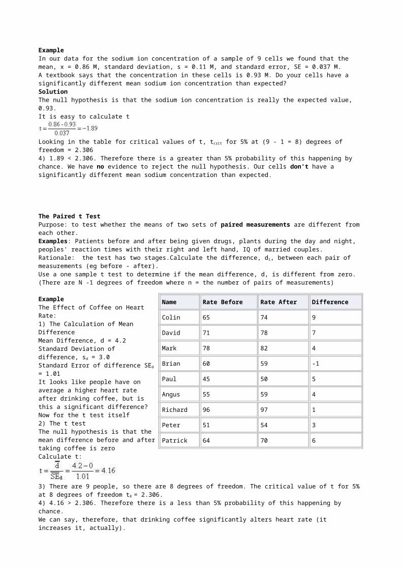
ExampleIn our data for the sodium ion concentration of a sample of 9 cells we found that the mean, x = 0.86 M, standard deviation, s = 0.11 M, and standard error, SE = 0.037 M. A textbook says that the concentration in these cells is 0.93 M. Do your cells have a significantly different mean sodium ion concentration than expected?SolutionThe null hypothesis is that the sodium ion concentration is really the expected value, 0.93.It is easy to calculate t

Looking in the table for critical values of t, tcrit for 5% at (9 - 1 = 8) degrees of freedom = 2.3064) 1.89 < 2.306. Therefore there is a greater than 5% probability of this happening by chance. We have no evidence to reject the null hypothesis. Our cells don't have a significantly different mean sodium concentration than expected.

The Paired t TestPurpose: to test whether the means of two sets of paired measurements are different from each other.Examples: Patients before and after being given drugs, plants during the day and night, peoples' reaction times with their right and left hand, IQ of married couples. Rationale: the test has two stages.Calculate the difference, di, between each pair of measurements (eg before - after).Use a one sample t test to determine if the mean difference, d, is different from zero. (There are N -1 degrees of freedom where n = the number of pairs of measurements)

ExampleThe Effect of Coffee on Heart Rate:1) The Calculation of Mean DifferenceMean Difference, d = 4.2Standard Deviation of difference, sd = 3.0Standard Error of difference SEd = 1.01It looks like people have on average a higher heart rate after drinking coffee, but is this a significant difference?Now for the t test itself2) The t testThe null hypothesis is that the mean difference before and after taking coffee is zeroCalculate t:

3) There are 9 people, so there are 8 degrees of freedom. The critical value of t for 5% at 8 degrees of freedom t8 = 2.306.4) 4.16 > 2.306. Therefore there is a less than 5% probability of this happening by chance.We can say, therefore, that drinking coffee significantly alters heart rate (it increases it, actually).

Name Rate Before Rate After Difference

Colin 65 74 9

David 71 78 7

Mark 78 82 4

Brian 60 59 -1

Paul 45 50 5

Angus 55 59 4

Richard 96 97 1

Peter 51 54 3

Patrick 64 70 6

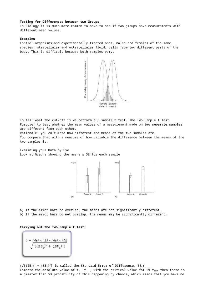
Testing for Differences between two GroupsIn Biology it is much more common to have to see if two groups have measurements with different mean values.

ExamplesControl organisms and experimentally treated ones, males and females of the same species, ntracellular and extracellular fluid, cells from two different parts of the body. This is difficult because both samples vary.

To tell what the cut-off is we perform a 2 sample t test. The Two Sample t TestPurpose: to test whether the mean values of a measurement made on two separate samples are different from each other.Rationale: you calculate how different the means of the two samples are. You compare that with a measure of how variable the difference between the means of the two samples is.

Examining your Data by EyeLook at Graphs showing the means ± SE for each sample

a) If the error bars do overlap, the means are not significantly different.b) If the error bars do not overlap, the means may be significantly different.

Carrying out the Two Sample t Test:

(√[(SE1)2 + (SE2)2] is called the Standard Error of Difference, SEd) Compare the absolute value of t, |t| , with the critical value for 5% tcrit then there is a greater than 5% probability of this happening by chance, which means that you have no evidence to reject the null hypothesis. If |t| > tcrit then there is a less than 5% probability of this happening by chance and you do have evidence to reject the null hypothesis and you can say the two means are significantly different from each other.

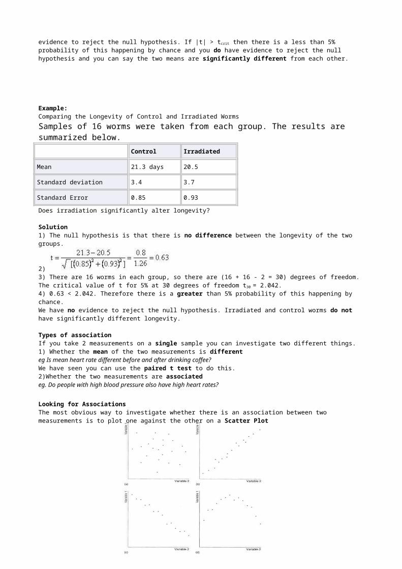
Example: Comparing the Longevity of Control and Irradiated WormsSamples of 16 worms were taken from each group. The results are summarized below.

Control Irradiated

Mean 21.3 days 20.5

Standard deviation 3.4 3.7

Standard Error 0.85 0.93

Does irradiation significantly alter longevity?

Solution1) The null hypothesis is that there is no difference between the longevity of the two groups.

2) 3) There are 16 worms in each group, so there are (16 + 16 - 2 = 30) degrees of freedom. The critical value of t for 5% at 30 degrees of freedom t30 = 2.042.4) 0.63 < 2.042. Therefore there is a greater than 5% probability of this happening by chance.We have no evidence to reject the null hypothesis. Irradiated and control worms do not have significantly different longevity.

Types of associationIf you take 2 measurements on a single sample you can investigate two different things.1) Whether the mean of the two measurements is differenteg Is mean heart rate different before and after drinking coffee? We have seen you can use the paired t test to do this.2)Whether the two measurements are associatedeg. Do people with high blood pressure also have high heart rates?

Looking for Associations The most obvious way to investigate whether there is an association between two measurements is to plot one against the other on a Scatter Plot

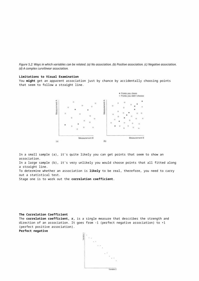
Figure 5.2: Ways in which variables can be related. (a) No association. (b) Positive association. (c) Negative association. (d) A complex curvilinear association.

Limitations to Visual ExaminationYou might get an apparent association just by chance by accidentally choosing points that seem to follow a straight line.

In a small sample (a), it's quite likely you can get points that seem to show an association.In a large sample (b), it's very unlikely you would choose points that all fitted along a straight line.To determine whether an association is likely to be real, therefore, you need to carry out a statistical test.Stage one is to work out the correlation coefficient.

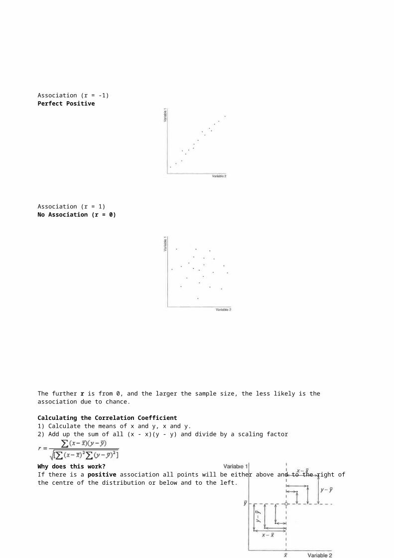
The Correlation Coefficient The correlation coefficient, r, is a single measure that describes the strength and direction of an association. It goes from -1 (perfect negative association) to +1 (perfect positive association).Perfect negative

Association (r = -1) Perfect Positive

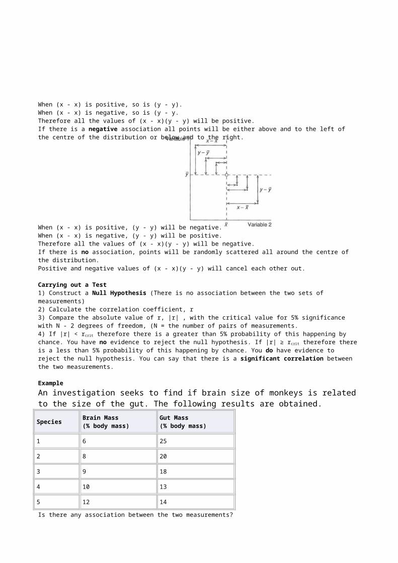
Association (r = 1)No Association (r = 0)

The further r is from 0, and the larger the sample size, the less likely is the association due to chance.

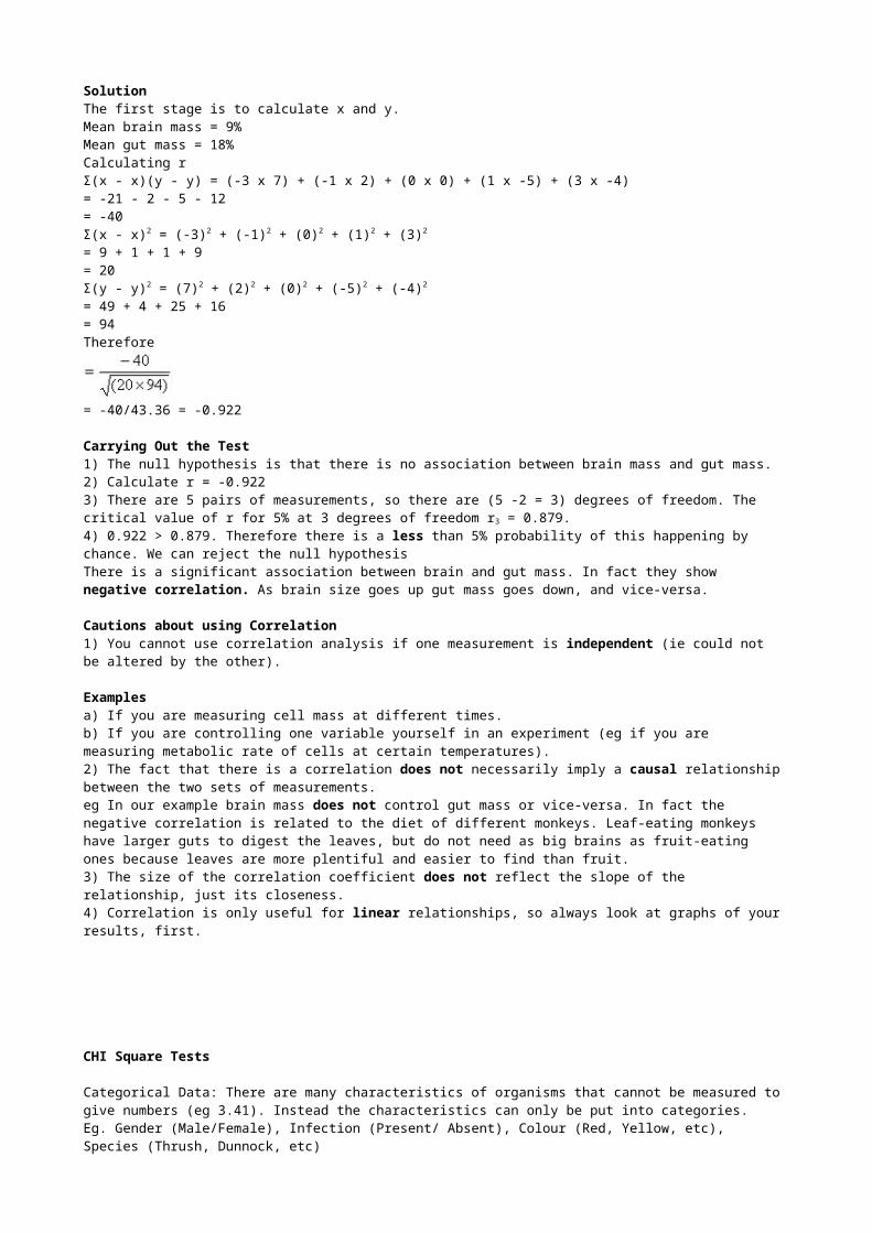
Calculating the Correlation Coefficient1) Calculate the means of x and y, x and y.2) Add up the sum of all (x - x)(y - y) and divide by a scaling factor

Why does this work?If there is a positive association all points will be either above and to the right of the centre of the distribution or below and to the left.

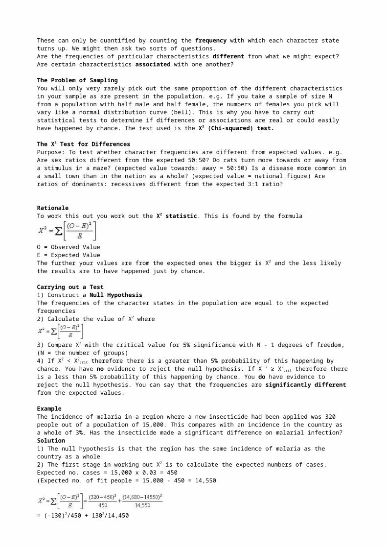
When (x - x) is positive, so is (y - y).When (x - x) is negative, so is (y - y.Therefore all the values of (x - x)(y - y) will be positive.If there is a negative association all points will be either above and to the left of the centre of the distribution or below and to the right.

When (x - x) is positive, (y - y) will be negative.When (x - x) is negative, (y - y) will be positive.Therefore all the values of (x - x)(y - y) will be negative.If there is no association, points will be randomly scattered all around the centre of the distribution.Positive and negative values of (x - x)(y - y) will cancel each other out.

Carrying out a Test1) Construct a Null Hypothesis (There is no association between the two sets of measurements)2) Calculate the correlation coefficient, r 3) Compare the absolute value of r, |r| , with the critical value for 5% significance with N - 2 degrees of freedom, (N = the number of pairs of measurements.4) If |r| < rcrit therefore there is a greater than 5% probability of this happening by chance. You have no evidence to reject the null hypothesis. If |r| ≥ rcrit therefore there is a less than 5% probability of this happening by chance. You do have evidence to reject the null hypothesis. You can say that there is a significant correlation between the two measurements.

ExampleAn investigation seeks to find if brain size of monkeys is related to the size of the gut. The following results are obtained.

SpeciesBrain Mass (% body mass)

Gut Mass (% body mass)

1 6 25

2 8 20

3 9 18

4 10 13

5 12 14

Is there any association between the two measurements?

SolutionThe first stage is to calculate x and y.Mean brain mass = 9%Mean gut mass = 18%Calculating rΣ(x - x)(y - y) = (-3 x 7) + (-1 x 2) + (0 x 0) + (1 x -5) + (3 x -4) = -21 - 2 - 5 - 12= -40

Σ(x - x)2 = (-3)2 + (-1)2 + (0)2 + (1)2 + (3)2 = 9 + 1 + 1 + 9= 20Σ(y - y)2 = (7)2 + (2)2 + (0)2 + (-5)2 + (-4)2 = 49 + 4 + 25 + 16= 94Therefore

= -40/43.36 = -0.922

Carrying Out the Test1) The null hypothesis is that there is no association between brain mass and gut mass.2) Calculate r = -0.9223) There are 5 pairs of measurements, so there are (5 -2 = 3) degrees of freedom. The critical value of r for 5% at 3 degrees of freedom r3 = 0.879.4) 0.922 > 0.879. Therefore there is a less than 5% probability of this happening by chance. We can reject the null hypothesisThere is a significant association between brain and gut mass. In fact they show negative correlation. As brain size goes up gut mass goes down, and vice-versa.

Cautions about using Correlation1) You cannot use correlation analysis if one measurement is independent (ie could not be altered by the other).

Examplesa) If you are measuring cell mass at different times.b) If you are controlling one variable yourself in an experiment (eg if you are measuring metabolic rate of cells at certain temperatures).2) The fact that there is a correlation does not necessarily imply a causal relationship between the two sets of measurements.eg In our example brain mass does not control gut mass or vice-versa. In fact the negative correlation is related to the diet of different monkeys. Leaf-eating monkeys have larger guts to digest the leaves, but do not need as big brains as fruit-eating ones because leaves are more plentiful and easier to find than fruit.3) The size of the correlation coefficient does not reflect the slope of the relationship, just its closeness.4) Correlation is only useful for linear relationships, so always look at graphs of your results, first.

CHI Square Tests

Categorical Data: There are many characteristics of organisms that cannot be measured to give numbers (eg 3.41). Instead the characteristics can only be put into categories. Eg. Gender (Male/Female), Infection (Present/ Absent), Colour (Red, Yellow, etc), Species (Thrush, Dunnock, etc) These can only be quantified by counting the frequency with which each character state turns up. We might then ask two sorts of questions.Are the frequencies of particular characteristics different from what we might expect? Are certain characteristics associated with one another?

The Problem of SamplingYou will only very rarely pick out the same proportion of the different characteristics in your sample as are present in the population. e.g. If you take a sample of size N from a population with half male and half female, the numbers of females you pick will vary like a normal distribution curve (bell). This is why you have to carry out statistical tests to determine if differences or associations are real or could easily have happened by chance. The test used is the X2 (Chi-squared) test.

The X2 Test for DifferencesPurpose: To test whether character frequencies are different from expected values. e.g. Are sex ratios different from the expected 50:50? Do rats turn more towards or away from a stimulus in a maze? (expected value towards: away = 50:50) Is a disease more common in a small town than in the nation as a whole? (expected value = national figure) Are ratios of dominants: recessives different from the expected 3:1 ratio?

RationaleTo work this out you work out the X2 statistic. This is found by the formula

O = Observed ValueE = Expected ValueThe further your values are from the expected ones the bigger is X2 and the less likely the results are to have happened just by chance.

Carrying out a Test1) Construct a Null Hypothesis The frequencies of the character states in the population are equal to the expected frequencies2) Calculate the value of X2 where

3) Compare X2 with the critical value for 5% significance with N - 1 degrees of freedom, (N = the number of groups)4) If X2 < X2

crit therefore there is a greater than 5% probability of this happening by chance. You have no evidence to reject the null hypothesis. If X 2 ≥ X2

crit therefore there is a less than 5% probability of this happening by chance. You do have evidence to reject the null hypothesis. You can say that the frequencies are significantly different from the expected values.

ExampleThe incidence of malaria in a region where a new insecticide had been applied was 320 people out of a population of 15,000. This compares with an incidence in the country as a whole of 3%. Has the insecticide made a significant difference on malarial infection? Solution1) The null hypothesis is that the region has the same incidence of malaria as the country as a whole.2) The first stage in working out X2 is to calculate the expected numbers of cases. Expected no. cases = 15,000 x 0.03 = 450(Expected no. of fit people = 15,000 - 450 = 14,550

= (-130)2/450 + 1302/14,450= 37.56 + 1.17 = 38.733) There are two groups (fit and ill) therefore 2 -1 degrees of freedom. X2

1 = 3.84.4) 38.73 > 3.84 therefore there is a significant difference in distribution. In fact there are fewer cases than expected

Warnings about Using X2 Tests 1) Never use percentages. Always use the actual frequencies. This is because bigger samples are less likely to differ by the same proportion from the expected value. E.g. you are quite likely to throw 2 heads: 0 tails.You are very unlikely to throw 100 heads: 0 tails2) Bigger sample sizes allow you to spot smaller differences (because of the squared term on top).3) Cases for which there is an expected outcome are very few and far between. eg If you examine the numbers of insects on flowers there is no reason to expect any particular ratio. Therefore there is another sort of test, the X2 test for associations

The X2 Test for AssociationsPurpose: To test whether two sets of character states are associated. E.g. Are particular species associated with particular habitats?Are particular diseases associated with particular racial groups? Are infections associated with particular groups of cells?Rationale: The test determines whether the distribution of character states is different from what it would be if they were randomly distributed around the population.

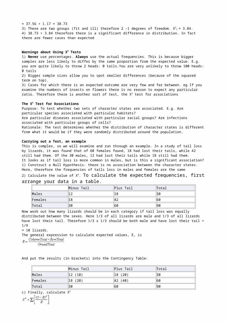
Carrying out a Test, an exampleThis is complex, so we will examine and run through an example. In a study of tail loss by lizards, it was found that of 60 females found, 18 had lost their tails, while 42 still had them. Of the 30 males, 12 had lost their tails while 18 still had them. It looks as if tail loss is more common in males, but is this a significant association?1) Construct a Null Hypothesis: there is no association between the character states. Here, therefore the frequencies of tails loss in males and females are the same2) Calculate the value of X2. To calculate the expected frequencies, first arrange your data in a table.

Minus Tail Plus Tail Total

Males 12 18 30

Females 18 42 60

Total 30 60 90

Now work out how many lizards should be in each category if tail loss was equally distributed between the sexes. Here 1/3 of all lizards are male and 1/3 of all lizards have lost their tail. Therefore 1/3 x 1/3 should be both male and have lost their tail = 1/9

= 10 lizards.The general expression to calculate expected values, E, is

And put the results (in brackets) into the Contingency Table:

Minus Tail Plus Tail Total

Males 12 (10) 18 (20) 30

Females 18 (20) 42 (40) 60

Total 30 60 90

c) Finally, calculate X2

= 0.4 + 0.2 + 0.2 + 0.1 = 0.73) Compare X2 with the critical value for 5% significance with (C - 1)(R - 1) degrees of freedom, (C and R are the numbers of columns and rows) Here there are (2 - 1)(2 - 1) = 1 degrees of freedomX2

1 = 3.84.4) If X2 < X2

crit therefore there is a greater than 5% probability of this happening by chance. You have no evidence to reject the null hypothesis. If X 2 ≥ X2

crit therefore there is a less than 5% probability of this happening by chance. Here 0.7 < 3.84, so we have no evidence to reject the null hypothesis. Despite what it looks like females are not significantly more likely to have intact tails.

Warnings about Using X2 Tests 1)Once again Never use percentages. Always use the actual frequencies.2) Expected totals should all be greater than 5, or else the test becomes less reliable. Therefore use as large samples as you can.

ANOVA

Often you might want to carry out rather more complex surveys or experiments. You might want to compare 2 experimentally treated groups of rats with a control group. You might want to compare people who have been put on 4 different drug regimes. You might want to compare 5 strains of bacteria. You might think you could carry out pairwise t tests, eg 1 vs 2, 1 vs 3, 2 vs 3But there are two problems, you would need to do lots of tests

Number of Groups 3 4 5 6 7 8 9 10

Number of Tests 3 6 10 16 23 31 40 50

Each time you perform a test there is a 5% probability of getting a significant answer by chance alone. Therefore the more tests you do the more likely you are to get a wrong answer.For this reason you must use a different test: Analysis of Variance or ANOVA

How ANOVA WorksThe t test compares the differences between 2 means with the pooled standard error of the means.ANOVA compares the amount of variability caused by the means being different with the amount of variability caused by points within each group being different from the mean.Take the simplest case of the weights of 2 group of fish (a) below.

The total variability (b) = The sum of squares of distances of points to the overall mean. The between group variability (c) = The sum of squares of distances of a point's group mean to the overall mean.The within group variability (d) = The sum of squares of distances of points to their group's mean.

Working out the MathematicsDoing the maths is actually rather complex, and involves several stages.1) Calculating the "Sums of Squares"a) The Total "Sum of Squares", SSt SSt = Σ so

2 Where so is the distance of each point to the overall mean.b) The Within Sample "Sum of Squares", SSw SSw =Σ sw

2 Where sw is the distance of each point to its group mean.c) The Between Sample "Sum of Squares", SSB SSB = SSt - SSw

We cannot compare these SS directly because they are the result of adding different numbers of points.

2) Calculating the Variance or Mean Squares. This is done by dividing by the correct numbers of degrees of freedom. a) Within Sample "Mean Square", MSw Where n = total number of points. N = number of groupsb) Between Sample "Mean Square", MSB

3) Calculating the ANOVA test statistic, F.The larger F is, the smaller the probability is of getting the results by chance if there were no difference between the groups Fortunately you don't have to work out F yourselves; it can all be done by SPSS.

Carrying Out an ANOVA TestConstruct a Null Hypothesis. Here the null hypothesis is that there is no difference between the groups. Enter your data in SPSS and use it to calculate the tests statistic, F. If Sig. > 0.05 therefore there is a greater than 5% probability of this happening by chance. You have no evidence to reject the null hypothesis. If Sig. ≤ 0.05 therefore there is a less than 5% probability of this happening by chance. You do have evidence to reject the null hypothesis

Working out Which Groups are DifferentThat's all fine but it doesn't tell you which groups are different from each other. To work this out, fortunately, you can use one of several Post Hoc tests - But only if the ANOVA shows a significant difference between groups. The Tukey and Scheffe tests compare each group with all the others. Dunnett's test compares a control group with each of the others. In our example there is no clear control, so we should use the Tukey test.

Regression

The bjectives of this Learning module are to test whether an apparent linear relationship between two variables is real, or whether it could have happened by chance because of variability. To do this one must use “Regression Analysis”. In an earlier unit we saw how correlation allows us to test for relationships between two measurements taken on the same items, both of which might be dependent on the other, eg Heart rate and blood pressure. However, there are many cases when one measurement is clearly independent of the other one, Eg Age and Mass of people: age is clearly independent of mass. Time and pH of cells: you look at the pH of cells at particular times. Reaction rate and temperature: you control the temperature and this affects the rate of reaction.You can't investigate these cases using correlation. Instead you must plot the data correctly and use regression analysis.

Plotting the Data

If between group variability is much greater than within group variability the two groups are probably different.Example:In a) the between group variability is much greater than the within group variability. There is a significant difference between the groups.

In b) the between group variability is much less than the within group variability. There is no significant difference between the groups.

You must plot the dependent variable on the y axis and the independent variable on the x axis. For instance the graph below shows how the mass of eggs depends on their age.

What Regression DoesRegression analysis calculates the "line of best fit" through the data points.

The ProblemYou could get the same equation just by chance even though the independent variable did not affect the dependent one, due to scatter.

Working out if Regressions are SignificantTo find if a regression line meaningfully represents your data, and explains much of the variability, you can use SPSS. It testsIf the slope of the line, b, is significantly different from 0If the intercept of the line, a, is significantly different from 0

Performing Your Own t TestsYou can also carry out your own t tests from the results of SPSS, to work out if the slope or intercept are different from any particular values, eg To test if eggs are significantly lighter than 90 g when they are laid (ie that the intercept < 90).The null hypothesis is that the eggs do weigh 90 g when laid.Calculate t using the equation

Compare t with the critical value for N - 2 degrees of freedom, where N = number of points. Here tcrit = 2.0690.247 < 2.069, so the difference is not significant. Initial weight is not significantly different from 90 g

This will help you to see how the dependent variable is affected by the independent variable.

It does it by working out the line, y = a + bx, which minimises the sum of the squares of the distances, si

2, of each point to the line.The slope, b, of the line is given by the equation

a is then calculated by putting the values of x, y and b into the equation y = a + bx.

a) In this case there is significant regression: Σsi2 is low

b) Here the regression is not significant: Σsi2 is high